Fast Policy Learning for Linear-Quadratic Control with Entropy Regularization

Abstract

This paper proposes and analyzes two new policy learning methods: regularized policy gradient (RPG) and iterative policy optimization (IPO), for a class of discounted linear-quadratic control (LQC) problems over an infinite time horizon with entropy regularization. Assuming access to the exact policy evaluation, both proposed approaches are proved to converge linearly in finding optimal policies of the regularized LQC. Moreover, the IPO method can achieve a super-linear convergence rate once it enters a local region around the optimal policy. Finally, when the optimal policy for an RL problem with a known environment is appropriately transferred as the initial policy to an RL problem with an unknown environment, the IPO method is shown to enable a super-linear convergence rate if the two environments are sufficiently close. Performances of these proposed algorithms are supported by numerical examples.

1 Introduction

Reinforcement Learning (RL) is a powerful framework for solving sequential decision-making problems, where a learning agent interacts with an unknown environment to improve her performance through trial and error [33]. In RL, an agent takes an action and receives a reinforcement signal in terms of a reward, which encodes the outcome of her action. In order to maximize the accumulated reward over time, the agent learns to select her actions based on her past experiences (exploitation) and/or by making new choices (exploration). Exploration and exploitation are the essence of RL, and entropy regularization has shown to be effective to balance the exploration-exploitation in RL, and more importantly to enable fast convergence [11, 17, 29].

Fast convergence and sample efficiency are critical for many applied RL problems, such as financial trading [19] and healthcare treatment recommendations [43], where acquiring new samples is costly or the chance of exploring new actions in the system is limited. In such cases, the cost of making incorrect decisions can be prohibitively high.

Our work.

This paper proposes and analyzes two new policy learning methods: regularized policy gradient (RPG) and iterative policy optimization (IPO), for a class of discounted entropy-regularized linear-quadratic control (LQC) problems over an infinite time horizon. Assuming access to the exact policy evaluation, both approaches are shown to converge linearly in finding optimal policies of the regularized LQC (Theorem 4.2 and 5.1). Moreover, the IPO method can achieve a super-linear convergence rate (on the order of one and a half) once it enters a local region around the optimal policy. Finally, when the optimal policy from an RL problem with a known environment is appropriately transferred as the initial policy to an RL problem with an unknown environment, the IPO algorithm is shown to enable a super-linear convergence rate if the two environments are sufficiently close (Theorem 6.1).

Our analysis approach is inspired by [12] to establish the gradient dominance condition within the linear-quadratic structure. Unlike theirs, our framework incorporates entropy regularization and state transition noise (Section 2). Therefore, in contrast to their deterministic and linear policies, our policies are of Gaussian type. Consequently, the gradient dominance condition involves both the gradient of the mean and the gradient of the covariance (Lemma 3.2). Accordingly, to establish the convergence of the covariance update in RPG, the smoothness of the objective function for bounded covariance is exploited, which is ensured with proper learning rate (Lemma 4.3).

Different from the first-order gradient descent update in most existing literature, our proposed IPO method requires solving an optimization problem at each step. This yields faster (super-linear) local convergence, established by bounding the differences between two discounted state correlation matrices with respect to the change in policy parameters (Lemma 5.4 and Theorem 5.3). This approach is connected intriguingly with [11], where the bound for the difference between discounted state visitation measures yielded the local quadratic convergence in Markov Decision Processes (MDPs).

Related works of policy gradient methods in LQC.

As a cornerstone in optimal control theory, the LQC problem is to find an optimal control in a linear dynamical system with a quadratic cost. LQC is popular due to its analytical tractability and its approximation power to nonlinear problems [3]. Until recently, most works on the LQC problem assumed that the model parameters are fully known. The first global convergence result for the policy gradient method to learn the optimal policy for LQC problems was developed in [12] for an infinite time horizon and with deterministic dynamics. Their work was extended in [6] to give global optimality guarantees of policy gradient methods for a larger class of control problems, which satisfy a closure condition under policy improvement and convexity of policy improvement steps. More progress has been made for policy gradient methods in other settings as well, including [7] for a real-valued matrix function, [8] for a continuous-time setting, [14] for multiplicative noise, [25], [27] for additive noise, and [18] for finite time horizon with an additive noise, [37] and [44] for time-average costs with risk constraints, [21] for nearly-linear dynamic system, [40] for distributional LQC to find the distribution of the return, and [20] for nonlinear stochastic control with exit time. Our work establishes fast convergence for both policy gradient based and policy optimization based algorithms for an infinite time horizon LQC with entropy regularization.

Related works of entropy regularization.

Entropy regularization has been frequently adopted to encourage exploration and improve convergence [16, 22, 23, 24, 31, 32, 38, 39, 42, 36, 35, 34, 28]. In particular, [2] showed that entropy regularization induces a smoother landscape that allows for the use of larger learning rates, and hence, faster convergence. Convergence rate analysis has been established when the underlying dynamic is an MDP with finite states and finite actions. For instance, [1] and [29] developed convergence guarantees for regularized policy gradient methods, with relative entropy regularization considered in [1] and entropy regularization in [29]. Both papers suggest the role of regularization in guaranteeing faster convergence for the tabular setting. For the natural policy gradient method, [11] established a global linear convergence rate and a local quadratic convergence rate.

For system with infinite number of states and actions, the closest to our work in terms of model setup is [39]. Our work replaces their aggregated control setup with controls that are randomly sampled from the policy, which are more realistic in handling real-world systems. The focuses of these two papers are also different: theirs explained the exploitation–exploration trade-off with entropy regularization from a continuous-time stochastic control perspective and provided theoretical support for Gaussian exploration for LQC; while ours is on algorithms design and the convergence analysis for discrete-time dynamics. It is worth noting that recently [13] showed the linear convergence rate of the policy gradient method under the framework of [39] with aggregated controls in continuous time. To the best of our knowledge, our work is the first non-asymptotic convergence result for discrete-time LQC with randomized controls under entropy regularization. In addition, we establish the first local super-linear convergence result under the LQC setting.

Related works of transfer learning.

Transfer learning, a.k.a. knowledge transfer, is a technique to utilize external expertise from other domains to benefit the learning process of a new task [9, 10, 30, 41]. It has gained popularity in many areas to improve the efficiency of learning. However, transfer learning in the RL framework is decisively more complicated and remains largely unexplored, as the knowledge to transfer involves a controlled stochastic process [45]. The transfer learning scheme proposed here is the first known theoretical development of transfer learning in the context of RL.

Notations and organization.

Throughout the paper, we will denote, for any matrix $Z\in\mathbb{R}^{m\times d}$, $Z^{\top}$ for the transpose of $Z$, $\|Z\|$ for the spectral norm of $Z$, $\|Z\|_{F}$ for the Frobenius norm of $Z$, $\operatorname{Tr}(Z)$ for the trace of a square matrix $Z$, and $\sigma_{\min}(Z)$ (resp. $\sigma_{\max}(Z)$) for the minimum (resp. maximum) singular value of a square matrix $Z$. We will adopt $\mathcal{N}(\mu,\Sigma)$ for a Gaussian distribution with mean $\mu\in\mathbb{R}^{d}$ and covariance matrix $\Sigma\in\mathbb{R}^{d\times d}$.

The rest of the paper is organized as follows. Section 2 introduces the problem and provides its theoretical solution using the dynamic programming principle. Section 3 presents the gradient dominance condition and related smoothness property. Section 4 introduces the RPG method and provides the global linear convergence result, and Section 5 proposes the IPO method, along with its global linear convergence and local super-linear convergence results. Section 6 shows that IPO leads to an efficient transfer learning scheme. Numerical examples are presented in Section 7.

Throughout this paper, proofs of main technical lemmas, unless otherwise specified, are deferred to Section 8.

2 Regularized LQC Problem and Solution

2.1 Problem Formulation

We consider an entropy-regularized LQC problem over an infinite time horizon with a constant discounted rate.

Randomized policy and entropy regularization.

To enable entropy regularization for exploration in the context of learning, we focus on randomized Markovian policies that are stationary. Namely, define the admissible policy set as $\Pi:=\Big{\{}\pi:\mathcal{X}\rightarrow\mathcal{P}(\mathcal{A})\Big{\}},$ with $\mathcal{X}$ the state space, $\mathcal{A}$ the action space, and $\mathcal{P}(\mathcal{A})$ the space of probability measures on action space $\mathcal{A}$. Here each admissible policy $\pi\in\Pi$ maps a state $x\in\mathcal{X}$ to a randomized action in $\mathcal{A}$.

For a given admissible policy $\pi\in\Pi$, the corresponding Shannon’s entropy is defined as

$$\mathcal{H}(\pi(\cdot|x)):=-\int_{\mathcal{A}}\log\pi(u|x)d\pi(u|x),\qquad\forall x\in\mathcal{X}.$$

The Shannon entropy quantifies the information gain from exploring the unknown environment. We incorporate this entropy term in the objective function as a regularization to encourage collecting information in the unknown environment and performing exploration.

Objective function and dynamics.

The decision maker aims to find an optimal policy by minimizing the following objective function

$$\min_{\pi\in\Pi}\,\mathbb{E}_{x\sim\mathcal{D}}[J_{\pi}(x)],$$ (1)

with value function $J_{\pi}$ given by

$$J_{\pi}(x):=\mathbb{E}_{\pi}\left.\left[\sum_{t=0}^{\infty}\gamma^{t}\left(x_{t}^{\top}Qx_{t}+u_{t}^{\top}Ru_{t}+\tau\log\pi(u_{t}|x_{t})\right)\right|x_{0}=x\right],$$ (2)

and for $t=0,1,2,\cdots$,

$$x_{t+1}=Ax_{t}+Bu_{t}+w_{t},\,x_{0}\sim\mathcal{D}.$$ (3)

Here $x_{t}\in\mathcal{X}:=\mathbb{R}^{n}$ is the state of the system and the initial state $x_{0}$ follows an initial distribution $\mathcal{D}$. Here $u_{t}\in\mathcal{A}:=\mathbb{R}^{k}$ is the control at time $t$ following a policy $\pi$. In addition, $\{w_{t}\}_{t=0}^{\infty}$ are zero-mean independent and identically distributed (i.i.d) noises. We assume that $\{w_{t}\}_{t=0}^{\infty}$ have finite second moments. That is, $\operatorname{Tr}(W)<\infty$ with $W:=\mathbb{E}[w_{t}w_{t}^{\top}]$ for any $t=0,1,2,\cdots$. The matrices $A\in\mathbb{R}^{n\times n},B\in\mathbb{R}^{n\times k}$ define the system’s (transition) dynamics. $Q\in\mathbb{R}^{n\times n}$ and $R\in\mathbb{R}^{k\times k}$ are matrices that parameterize the quadratic costs. $\gamma\in(0,1)$ denotes the discount factor and $\tau>0$ denotes the regularization parameter. The expectation in (2) is taken with respect to the control $u_{t}\sim\pi(\cdot|x_{t})$ and system noise $w_{t}$ for $t\geq 0$.

2.2 Optimal Value Function and Policy

While the optimal solution to the LQC problem is a well-explored topic, it is worth noting that, to the best of our knowledge, no prior work has presented a solution to the entropy-regularized LQC problem in the form of (2). Additionally, in the study of [39] for entropy-regularized LQC with continuous-time state dynamics, they focused on the state transitions with aggregated controls. This differs from the state transitions considered in (3), where the controls in the state transitions are randomly sampled from the policy $\pi$.

Optimal value function.

The optimal value function $J^{*}:\mathcal{X}\rightarrow\mathbb{R}$ is defined as

$$J^{*}(x)=\min_{\pi\in\Pi}J_{\pi}(x).$$ (4)

The following theorem establishes the explicit expression for the optimal control policy and the corresponding optimal value function: the optimal policy is characterized as a multivariate Gaussian distribution, with the mean linear in the state $x$ and a constant covariance matrix.

Theorem 2.1 (Optimal value functions and optimal policy).

The optimal value function $J^{*}:\mathcal{X}\rightarrow\mathbb{R}$ in (4) can be expressed as $J^{*}(x)=x^{\top}Px+q$ with $P$ and $q$ satisfying

$$P =Q+K^{*\top}RK^{*}+\gamma(A-BK^{*})^{\top}P(A-BK^{*}),$$ (5)

$$q =\frac{1}{1-\gamma}\Big{[}\operatorname{Tr}(\Sigma^{*}(R+\gamma B^{\top}PB))-\frac{\tau}{2}\left(k+\log\left((2\pi)^{k}\operatorname{det}\Sigma^{*}\right)\right)+\gamma\operatorname{Tr}(WP)\Big{]},$$

where

$$K^{*}=\gamma(R+\gamma B^{\top}PB)^{-1}B^{\top}PA,\quad\Sigma^{*}=\frac{\tau}{2}(R+\gamma B^{\top}PB)^{-1}.$$ (6)

For any $x\in\mathcal{X}$, the corresponding optimal policy $\pi^{*}$ to (4) is a Gaussian policy: $\pi^{*}(\cdot|x)=\mathcal{N}(-K^{*}x,\Sigma^{*}).$

Proof of Theorem 2.1 relies on the following lemma, which establishes the optimal solution for the one-step reward function, given the presence of entropy regularization in the reward.

Lemma 2.2.

For any given symmetric positive definite matrix $M\in\mathbb{R}^{k\times k}$ and vector $b\in\mathbb{R}^{k}$, the optimal solution $p^{*}\in\mathcal{P}(\mathcal{A})$ to the following optimization problem is a multivariate Gaussian distribution with covariance $\frac{\tau}{2}M^{-1}$ and mean $-\frac{1}{2}M^{-1}b$:

$$\min_{p\in\mathcal{P}(\mathcal{A})} \mathbb{E}_{u\sim p(\cdot)}\left[u^{\top}Mu+b^{\top}u+\tau\log p(u)\right],$$

subject to $$\int_{\mathcal{A}}p(u)du=1,$$

$$p(u)\geq 0,\quad\forall u\in\mathcal{A}.$$

Proof.

(of Theorem 2.1). By definition of $J^{*}$ in (4),

$$J^{*}(x)=\min_{\pi\in\Pi}\mathbb{E}_{\pi}\Bigl{\{}x^{\top}Qx+u^{\top}Ru+\tau\log(\pi(u|x))+\gamma J^{*}(Ax+Bu+w)\Bigr{\}},$$ (7)

where the expectation is taken with respect to $u\sim\pi(\cdot|x)$ and the noise term $w$, with mean $0$ and covariance $W$. Stipulating

$$J^{*}(x)=x^{\top}Px+q$$ (8)

for a positive definite $P\in\mathbb{R}^{n\times n}$ and $q\in\mathbb{R}$ and plugging into (7), we can obtain the optimal value function with dynamic programming principle [4, 5, 15, 33]:

$$J^{*}(x) =x^{\top}Qx$$

$$\quad+\min_{\pi}\mathbb{E}_{\pi}\Bigl{\{}u^{\top}Ru+\tau\log(\pi(u|x))+\gamma\left[(Ax+Bu+w)^{\top}P(Ax+Bu+w)+q\right]\Bigr{\}}$$

$$=x^{\top}Qx+\gamma\operatorname{Tr}(WP)+\gamma x^{\top}A^{\top}PAx+\gamma q$$

$$\quad+\min_{\pi}\mathbb{E}_{\pi}\Bigl{\{}u^{\top}(R+\gamma B^{\top}PB)u+\tau\log(\pi(u|x))+2\gamma u^{\top}B^{\top}PAx\Bigr{\}}.$$ (9)

Now apply Lemma 2.2 to (9) with $M=R+\gamma B^{\top}PB$ and $b=2\gamma B^{\top}PAx$, one can get the optimal policy at state $x$:

$$\pi^{*}(\cdot|x) =\mathcal{N}\left(-\gamma(R+\gamma B^{\top}PB)^{-1}B^{\top}PAx,\frac{\tau}{2}(R+\gamma B^{\top}PB)^{-1}\right)$$ (10)

$$=\mathcal{N}\left(-K^{*}x,\Sigma^{*}\right),$$ (11)

where $K^{*},\Sigma^{*}$ are defined in (6). To derive the associated optimal value function, we first calculate the negative entropy of policy $\pi^{*}$ at any state $x\in\mathcal{X}$:

$$\mathbb{E}_{\pi^{*}}[\log(\pi^{*}(u|x))]=\int_{\mathcal{A}}\log(\pi^{*}(u|x))\pi^{*}(u|x)du=-\frac{1}{2}\left(k+\log\left((2\pi)^{k}\operatorname{det}\Sigma^{*}\right)\right).$$ (12)

Plug (10) and (12) into (9) to get

$$J^{*}(x)= x^{\top}\left(Q+K^{*\top}RK^{*}+\gamma(A-BK^{*})^{\top}P(A-BK^{*})\right)x$$

$$+\text{Tr}(\Sigma^{*}R)-\frac{\tau}{2}\left(k+\log\left((2\pi)^{k}\operatorname{det}\Sigma^{*}\right)\right)+\gamma\left(\text{Tr}(\Sigma^{*}B^{\top}PB)+\text{Tr}(WP)+q\right).$$

Combining this with (8), the proof is complete. ∎

3 Analysis of Value Function and Policy Gradient

In this section, we analyze the expression of the policy gradient, the gradient dominance condition, and the smoothness property of the value function. These properties are necessary for studying the algorithms proposed in Section 4 and Section 5.

Throughout the analysis, we assume that there exists $\rho\in(0,\frac{1}{\sqrt{\gamma}})$ satisfying $\|A-BK^{*}\|\leq\rho$ where $K^{*}$ is the optimal solution in Theorem 2.1. We consider the following domain $\Omega$ (i.e., the admissible control set) for $(K,\Sigma)$: $\Omega=\{K\in\mathbb{R}^{k\times n},\Sigma\in\mathbb{R}^{k\times k}:\|A-BK\|\leq\rho,\Sigma\succ 0,\Sigma^{\top}=\Sigma\}.$ For any $x_{0}\in\mathcal{X}$ following the initial distribution $\mathcal{D}$, we assume that $\mathbb{E}_{x_{0}\sim\mathcal{D}}[x_{0}x_{0}^{\top}]$ exists and $\mu:=\sigma_{\min}\left(\mathbb{E}_{x_{0}\sim\mathcal{D}}[x_{0}x_{0}^{\top}]\right)>0.$ For any $(K,\Sigma)\in\Omega$, define $S_{K,\Sigma}$ as the discounted state correlation matrix, i.e.,

$$S_{K,\Sigma}:=\mathbb{E}_{\pi_{K,\Sigma}}\left[\sum_{i=0}^{\infty}\gamma^{i}x_{i}x_{i}^{\top}\right].$$ (13)

According to Theorem 2.1, the optimal policy of (1) is a Gaussian policy with a mean following a linear function of the state and a constant covariance matrix. In the remainder of the paper, we look for a parameterized policy of the form

$$\pi_{K,\Sigma}(\cdot|x):=\mathcal{N}(-Kx,\Sigma),$$ (14)

for any $x\in\mathcal{X}$. With a slight abuse of notation, we use $J_{K,\Sigma}$ to denote $J_{\pi_{K,\Sigma}}$ and denote the objective in (1) as a function of $(K,\Sigma)$, given by

$$C(K,\Sigma):=\mathbb{E}_{x\sim\mathcal{D}}\left[J_{K,\Sigma}(x)\right].$$ (15)

To analyze the dependence of $\Sigma$ in the objective function (15) for any fixed $K$, we also define $f_{K}:\mathbb{R}^{k\times k}\rightarrow\mathbb{R}$ as

$$f_{K}({\Sigma})=\frac{\tau}{2(1-\gamma)}\log\operatorname{det}({\Sigma})-\frac{1}{1-\gamma}\operatorname{Tr}\left({\Sigma}(R+\gamma B^{\top}P_{K}B)\right),\quad\forall\,{\Sigma}\succ 0.$$ (16)

By applying the Bellman equation, we can get $J_{K,\Sigma}(x)=x^{\top}P_{K}x+q_{K,\Sigma}$ with some symmetric positive definite matrix $P_{K}\in\mathbb{R}^{n\times n}$ and $q_{K,\Sigma}\in\mathbb{R}$ satisfying

$$P_{K} =Q+K^{\top}RK+\gamma(A-BK)^{\top}P_{K}(A-BK),$$ (17)

$$q_{K,\Sigma} =\frac{1}{1-\gamma}\Big{[}\operatorname{Tr}(\Sigma(R+\gamma B^{\top}P_{K}B)-\frac{\tau}{2}\left(k+\log\left((2\pi)^{k}\operatorname{det}\Sigma\right)\right)+\gamma\operatorname{Tr}(WP_{K})\Big{]}.$$

Note that (17) differs from equations (5) in terms of their solutions. In (5), the values of $K^{*}$ and $\Sigma^{*}$ are explicitly defined by $K^{*}=\gamma(R+\gamma B^{\top}PB)^{-1}B^{\top}PA$ and $\Sigma^{*}=\frac{\tau}{2}(R+\gamma B^{\top}PB)^{-1}$. By substituting these values into (5), one can obtain the solutions for $P$ and $q$, which define the optimal value function $J^{*}(x)=x^{\top}Px+q$.

Meanwhile, $K$ and $\Sigma$ in (17) can take any admissible policy parameter values in $\Omega$, and the resulting $P_{K}$ and $q_{K,\Sigma}$ are functions of these policy parameters. The value function $J_{K,\Sigma}(x)$ derived from (17) represents the value starting from the state $x$ with the policy parameters $(K,\Sigma)$, which may or may not correspond to an optimal policy.

We now provide an explicit form for the gradient of the cost function $C(K,\Sigma)$ with respect to $K$ and $\Sigma$. This explicit form will be used to show the gradient dominance condition in Lemma 3.2 and also in analyzing the algorithms in Sections 4 and 5.

Lemma 3.1 (Explicit form for the policy gradient).

Take a policy in the form of (14) with parameter $(K,\Sigma)\in\Omega$, then the policy gradient has the following explicit form:

$$\nabla_{K}C(K,\Sigma) =2E_{K}S_{K,\Sigma},\quad\nabla_{\Sigma}C(K,\Sigma)=(1-\gamma)^{-1}\left(R-\frac{\tau}{2}\Sigma^{-1}+\gamma B^{\top}P_{K}B\right),$$ (18)

where $E_{K}:=-\gamma B^{\top}P_{K}(A-BK)+RK$ and $S_{K,\Sigma}$ is defined in (13).

Gradient dominance.

To prove the global convergence of policy gradient methods, the key idea is to show the gradient dominance condition, which states that $C(K,\Sigma)-C(K^{*},\Sigma^{*})$ can be bounded by $\|\nabla_{K}C(K,\Sigma)\|_{F}^{2}$ and $\|\nabla_{\Sigma}C(K,\Sigma)\|_{F}^{2}$ for any $(K,\Sigma)\in\Omega$. This suggests that when the gradient norms are sufficiently small, the cost function of the given policy is sufficiently close to the optimal cost function.

Lemma 3.2 (Gradient dominance of $C(K,\Sigma)$).

Let $\pi^{*}$ be the optimal policy with parameters $K^{*},\Sigma^{*}$. Suppose policy $\pi$ with parameter $(K,\Sigma)\in\Omega$ satisfying $\Sigma\preceq I$ has a finite expected cost, i.e., $C(K,\Sigma)<\infty$. Then

$$C(K,\Sigma)-C(K^{*},\Sigma^{*})\leq\frac{\|S_{K^{*},\Sigma^{*}}\|}{4\mu^{2}\sigma_{\min}(R)}\|\nabla_{K}C(K,\Sigma)\|_{F}^{2}+\frac{1-\gamma}{\sigma_{\min}(R)}\|\nabla_{\Sigma}C(K,\Sigma)\|_{F}^{2}.$$ (19)

For a lower bound, with $E_{K}$ defined in Lemma 3.1,

$$C(K,\Sigma)-C(K^{*},\Sigma^{*})\geq\frac{\mu}{\|R+\gamma B^{\top}P_{K}B\|}\operatorname{Tr}(E_{K}^{\top}E_{K}).$$

“Almost” smoothness.

Next, we will develop a smoothness property for the cost objective $C(K,\Sigma)$, which is necessary for establishing the convergence algorithms proposed in Section 4 and Section 5.

A function $f:\mathbb{R}^{n}\rightarrow\mathbb{R}$ is considered smooth if the following condition is satisfied [12, 18]:

$$\left|f(x)-f(y)+\nabla f(x)^{\top}(y-x)\right|\leq\frac{m}{2}\|x-y\|^{2},\quad\forall x,y\in\mathbb{R}^{n},$$

with $m$ a finite constant. In general, characterizing the smoothness of $C(K,\Sigma)$ is challenging, as it may become unbounded when the eigenvalues of $A-BK$ exceed $\frac{1}{\sqrt{\gamma}}$ or when $\sigma_{\min}(\Sigma)$ is close to $0$. Nevertheless, in Lemma 3.3, we will see that if $C(K,\Sigma)$ is “almost” smooth, then the difference $C(K,\Sigma)-C(K^{\prime},\Sigma^{\prime})$ can be bounded by the sum of linear and quadratic terms involving $K-K^{\prime}$ and $\Sigma-\Sigma^{\prime}$.

Lemma 3.3 (“Almost” smoothness of $C(K,\Sigma)$).

Fix $0<a\leq 1$ and define $M_{a}=\frac{\tau\left(-\log\left(a\right)+a-1\right)}{2(1-\gamma)\left(a-1\right)^{2}}$. For any $K,\Sigma$ and $K^{\prime},\Sigma^{\prime}$ satisfying $aI\preceq\Sigma\preceq I$ and $aI\preceq\Sigma^{\prime}\preceq I$,

$$C(K^{\prime},\Sigma^{\prime})-C(K,\Sigma)=\operatorname{Tr}\left(S_{K^{\prime},\Sigma^{\prime}}(K^{\prime}-K)^{\top}(R+\gamma B^{\top}P_{K}B)(K^{\prime}-K)\right)$$

$$\quad+2\operatorname{Tr}\left(S_{K^{\prime},\Sigma^{\prime}}(K^{\prime}-K)^{\top}E_{K}\right)+f_{K}(\Sigma)-f_{K}(\Sigma^{\prime})$$

$$\leq\operatorname{Tr}\left(S_{K^{\prime},\Sigma^{\prime}}(K^{\prime}-K)^{\top}(R+\gamma B^{\top}P_{K}B)(K^{\prime}-K)\right)+2\operatorname{Tr}\left(S_{K^{\prime},\Sigma^{\prime}}(K^{\prime}-K)^{\top}E_{K}\right)$$

$$\quad+\frac{1}{1-\gamma}\operatorname{Tr}\left(\left(R+\gamma B^{\top}P_{K}B-\frac{\tau}{2}\Sigma^{-1}\right)(\Sigma^{\prime}-\Sigma)\right)+M_{a}\operatorname{Tr}\left((\Sigma^{-1}\Sigma^{\prime}-I)^{2}\right),$$

where $f_{K}$ is defined in (16).

4 Regularized Policy Gradient Method

In this section, we propose a new regularized policy gradient (RPG) update for the parameters $K$ and $\Sigma$:

$$K^{(t+1)} =K^{(t)}-\eta_{1}\nabla_{K}C\left(K^{(t)},\Sigma^{(t)}\right)\cdot\left(S_{K^{(t)},\Sigma^{(t)}}\right)^{-1},$$

$$\Sigma^{(t+1)} =\Sigma^{(t)}-\eta_{2}\Sigma^{(t)}\nabla_{\Sigma}C\left(K^{(t)},\Sigma^{(t)}\right)\Sigma^{(t)}.$$

RPG takes into account the inherent structure of the parameter space, which can accelerate convergence.

By the explicit expressions of $\nabla_{K}C(K,\Sigma)$ and $\nabla_{\Sigma}C(K,\Sigma)$ in (18), the above update is equivalent to

$$K^{(t+1)} =K^{(t)}-2\eta_{1}E_{K^{(t)}},$$ (RPG)

$$\Sigma^{(t+1)} =\Sigma^{(t)}-\frac{\eta_{2}}{1-\gamma}\Sigma^{(t)}\left({R}+\gamma B^{\top}P_{K^{(t)}}B-\frac{\tau}{2}{\left(\Sigma^{(t)}\right)}^{-1}\right)\Sigma^{(t)}.$$

From (RPG), one can see that the update of parameter $K$ does not depend on the covariance matrix $\Sigma$. However, the update of $\Sigma$ does depend on $K$ through $P_{K}$.

Remark 4.1 (Comparison to natural policy gradient).

Assume that the covariance matrix $\Sigma$ is parameterized as scalar multiplication of an identity matrix, i.e., $\Sigma=sI$ for some $s>0$ and

$$\pi_{K,s}(x,u)=\mathcal{N}(Kx,sI).$$ (20)

Then the natural policy gradient follows the update [26]:

$$K^{\prime} =K-\eta G_{K}^{-1}\nabla C(K,sI),\,\,s^{\prime}=s-\eta G_{s}^{-1}\partial_{s}C(K,sI),$$

where

$$G_{K}=\mathbb{E}\left[\sum_{t=0}^{\infty}\,\nabla\log\pi_{K,s}(u_{t}|x_{t})\nabla\log\pi_{K,s}(u_{t}|x_{t})^{\top}\right],$$ (21)

$$G_{s}=\mathbb{E}\left[\sum_{t=0}^{\infty}\,\partial_{s}\log\pi_{K,s}(u_{t}|x_{t})\partial_{s}\log\pi_{K,s}(u_{t}|x_{t})^{\top}\right]$$ (22)

is the Fischer information matrix under policy $\pi_{K,s}$. When the covariance matrix of the Gaussian policy takes a diagonal form as in (20), (4.1) and (22) are equivalent to

$$K^{\prime}=K-\eta\nabla C(K,sI)(S_{K,sI})^{-1},\quad s^{\prime}=s-\tilde{\eta}~{}\partial_{s}C(K,sI)s^{2},$$ (23)

for some constant $\tilde{\eta}>0$.

Even though (RPG) is similar to (23), there is no corresponding Fisher information form associated with (RPG) because of the additional step that simultaneously updates the covariance matrix $\Sigma$, which may not necessarily be diagonal.

We next show that (RPG) achieves a linear convergence rate. The covariance matrices $\left\{\Sigma^{(t)}\right\}_{t=0}^{\infty}$ using (RPG) remain bounded, provided that the initial covariance matrix $\Sigma^{(0)}$ is appropriately bounded.

Theorem 4.2 (Global convergence of (RPG)).

Given $\tau\in(0,2\sigma_{\min}(R)],$ take $(K^{(0)},\Sigma^{(0)})\in\Omega$ such that $\Sigma^{(0)}\preceq I$. Define $M_{\tau}:=\frac{\tau k}{2(1-\gamma)}\log\left(\frac{\sigma_{\min}(R)}{\pi\tau}\right)$ and

$$r_{0}:=\max\left\{\frac{2}{\tau\sigma_{\min}\left(\Sigma^{(0)}\right)},\,\|R\|+\gamma\frac{\|B^{\top}B\|\left(C(K^{(0)},\Sigma^{(0)})-M_{\tau}\right)}{\mu+\frac{\gamma}{1-\gamma}\sigma_{\min}(W)}\right\}.$$

Then for $\eta_{1},\eta_{2}=\frac{1}{2r_{0}},\frac{\tau(1-\gamma)}{2r_{0}^{2}}$ and for

$$N\geq\max\left\{\frac{\|S_{K^{*},\Sigma^{*}}\|r_{0}}{\mu\sigma_{\min}(R)},\frac{8r_{0}^{3}}{\tau^{2}\sigma_{\min}(R)}\right\}\log\frac{C(K^{(0)},\Sigma^{(0)})-C(K^{*},\Sigma^{*})}{\varepsilon},$$

the regularized policy gradient descent (RPG) has the following performance bound:

$$C\left(K^{(N)},\Sigma^{(N)}\right)-C(K^{*},\Sigma^{*})\leq\varepsilon.$$

To prove Theorem 4.2, we will first need the boundedness of the one-step update of the covariance $\Sigma$, in order to guarantee the well-definedness of the cost function along the trajectory when performing (RPG) (Lemma 4.3). Additionally, we will bound the one-step update of (RPG) (Lemma 4.4), and provide an upper bound of $\|P_{K}\|$ in terms of the objective function $C(K,\Sigma)$ (Lemma 4.5).

Lemma 4.3 (Boundedness of the update of $\Sigma$ in (RPG)).

Let $(K,\Sigma)\in\Omega$ be given such that $0\prec\Sigma\preceq I$. Assume $\tau\in(0,\,2\sigma_{\min}(R)]$. Fix $a\in\left(0,\,\min\left\{\frac{\tau}{2\|R+\gamma B^{\top}P_{K}B\|},\sigma_{\min}(\Sigma)\right\}\right).$ Let $K^{\prime},\Sigma^{\prime}$ be the one-step update of $K,\Sigma$ using (RPG) with $\eta_{2}\leq\frac{2(1-\gamma)a^{2}}{\tau}$. Then $aI\preceq\Sigma^{\prime}\preceq I$.

Lemma 4.4 (Contraction of (RPG)).

Let $(K,\Sigma)\in\Omega$ be given such that $0\prec\Sigma\preceq I$. Assume $\tau\in(0,2\sigma_{\min}(R)]$. Fix $a\in\left(0,\,\min\left\{\frac{\tau}{2\|R+\gamma B^{\top}P_{K}B\|},\sigma_{\min}(\Sigma)\right\}\right).$ Let $K^{\prime},\Sigma^{\prime}$ be the one-step update of $K,\Sigma$ using (RPG) with $\eta_{1}\leq\frac{1}{2\|R+\gamma B^{\top}P_{K}B\|},\eta_{2}\leq\frac{2(1-\gamma)a^{2}}{\tau}$. Then $aI\preceq\Sigma^{\prime}\preceq I$ and

$$C(K^{\prime},\Sigma^{\prime})-C(K^{*},\Sigma^{*})\leq(1-\zeta)(C(K,\Sigma)-C(K^{*},\Sigma^{*})),$$

with $0<\zeta=\min\left\{\frac{2\mu\eta_{1}\sigma_{\min}(R)}{\|S_{K^{*},\Sigma^{*}}\|},\frac{\eta_{2}a\sigma_{\min}(R)}{2(1-\gamma)}\right\}<1.$

Lemma 4.5 (Lower bound for $C(K,\Sigma)$).

Let $M_{\tau}$ be defined in the same way as in Theorem 4.2. Then for all $(K,\Sigma)\in\Omega$,

$$C(K,\Sigma)\geq\left(\mu+\frac{\gamma}{1-\gamma}\sigma_{\min}(W)\right)\|P_{K}\|+M_{\tau}.$$

Proof.

(of Theorem 4.2). Using Lemma 4.5 for any $t\geq 0,$

$$\frac{1}{\left\|R+\gamma B^{\top}P_{K^{(t)}}B\right\|}\geq\frac{1}{\|R\|+\gamma\|B^{\top}B\|\left\|P_{K^{(t)}}\right\|}\geq\frac{1}{\|R\|+\gamma\frac{\|B^{\top}B\|\left(C({K^{(t)}},\Sigma^{(t)})-M_{\tau}\right)}{\mu+\frac{\gamma}{1-\gamma}\sigma_{\min}(W)}}.$$ (24)

Let $a=\frac{\tau}{2r_{0}}$, $\zeta=\min\left\{\frac{2\mu\eta_{1}\sigma_{\min}(R)}{\|S_{K^{*},\Sigma^{*}}\|},\frac{\eta_{2}a\sigma_{\min}(R)}{2(1-\gamma)}\right\}$. The proof is completed by induction to show $C(K^{(t+1)},\Sigma^{(t+1)})\leq(1-\zeta)C(K^{(t)},\Sigma^{(t)})$ and $aI\preceq\Sigma^{(t+1)}\preceq I$ holds for all $t\geq 0$: at $t=0$, apply (24) to get $\eta_{1}\leq\frac{1}{2\|R+\gamma B^{\top}P_{K^{(0)}}B\|}$ and $a\leq\frac{\tau}{2\|R+\gamma B^{\top}P_{K^{(0)}}B\|}$. Additionally with $\eta_{2}=\frac{\tau(1-\gamma)}{2r_{0}^{2}}=\frac{2(1-\gamma)a^{2}}{\tau}$ and $aI\preceq\Sigma^{(0)}\preceq I$, Lemma 4.4 can be applied to get

$$C(K^{(1)},\Sigma^{(1)})\leq(1-\zeta)C(K^{(0)},\Sigma^{(0)})\leq C(K^{(0)},\Sigma^{(0)}),$$

and $aI\preceq\Sigma^{(1)}\preceq I$. The proof proceeds by arguing that Lemma 4.4 can be applied at every step. If it were the case that $C\left(K^{(t)},\Sigma^{(t)}\right)\leq(1-\zeta)C\left(K^{(t-1)},\Sigma^{(t-1)}\right)\leq C\left(K^{(0)},\Sigma^{(0)}\right)$ and $aI\preceq\Sigma^{(t)}\preceq I$, then

$$2\eta_{1} =\frac{1}{\|R\|+\gamma\frac{\|B^{\top}B\|\left(C(K^{(0)},\Sigma^{(0)})-M_{\tau}\right)}{\mu+\frac{\gamma}{1-\gamma}\sigma_{\min}(W)}}\leq\frac{1}{\|R\|+\gamma\frac{\|B^{\top}B\|\left(C\left(K^{(t)},\Sigma^{(t)}\right)-M_{\tau}\right)}{\mu+\frac{\gamma}{1-\gamma}\sigma_{\min}(W)}}$$

$$\overset{\eqref{eqn: eta 1 in a thm}}{\leq}\frac{1}{\left\|R+\gamma B^{\top}P_{K^{(t)}}B\right\|},$$

and in the same way one could get $a\leq\frac{\tau}{2\left\|R+\gamma B^{\top}P_{K^{(t)}}B\right\|}$. Thus, Lemma 4.4 can be applied such that

$$C\left(K^{(t+1)},\Sigma^{(t+1)}\right)-C(K^{*},\Sigma^{*})\leq(1-\zeta)\left(C\left(K^{(t)},\Sigma^{(t)}\right)-C(K^{*},\Sigma^{*})\right).$$

and $aI\preceq\Sigma^{(t+1)}\preceq I.$ Thus, the induction is complete. Finally, observe that $0<\zeta\leq\frac{2\mu\eta_{1}\sigma_{\min}(R)}{\|S_{K^{*},\Sigma^{*}}\|}=\frac{\mu\sigma_{\min}(R)}{\|S_{K^{*},\Sigma^{*}}\|r_{0}}<1,\text{ and }\zeta\leq\frac{\eta_{2}a\sigma_{\min}(R)}{2(1-\gamma)}=\frac{\tau^{2}\sigma_{\min}(R)}{8r_{0}^{3}},$ the proof is complete.∎

5 Iterative Policy Optimization Method

In this section, we propose an iterative policy optimization method (IPO), in which we optimize a one-step deviation from the current policy in each iteration. For IPO, one can show both the global convergence with a linear rate and a local super-linear convergence when the initialization is close to the optimal policy. This local super-linear convergence result benefits from the entropy regularization.

By Bellman equation for the value function $J_{K,\Sigma}$,

$$J_{K,\Sigma}(x)=\mathbb{E}_{u\sim\pi_{K,\Sigma}}\Big{[} x^{\top}Qx+u^{\top}Ru+\tau\log\pi_{K,\Sigma}(u|x)+\gamma J_{K,\Sigma}(Ax+Bu+w)\Big{]}.$$

We assume the one-step update $(K^{\prime},\Sigma^{\prime})$ satisfies:

$$K^{\prime},\Sigma^{\prime}=\arg\min_{\widetilde{K},\widetilde{\Sigma}}\mathbb{E}_{u\sim\pi_{\widetilde{K},\widetilde{\Sigma}}}\Big{[}x^{\top}Qx+u^{\top}Ru+\tau\log\pi_{\widetilde{K},\widetilde{\Sigma}}(u|x)+\gamma{J_{K,\Sigma}}(Ax+Bu+w)\Big{]}$$

By direct calculation, we have the following explicit forms for the updates:

$$K^{(t+1)} =K^{(t)}-\left(R+\gamma B^{\top}P_{K^{(t)}}B\right)^{-1}E_{K^{(t)}},$$ (IPO)

$$\Sigma^{(t+1)} =\frac{\tau}{2}\left(R+\gamma B^{\top}P_{K^{(t)}}B\right)^{-1},$$

for $t=1,2,\cdots.$ The update of $K$ in (IPO) is identical to the Gauss-Newton update when the learning rate is equal to $1$ in [12]. The update of $\Sigma$ in (IPO) is not gradient-based and only depends on the value of $K$ in the previous step.

5.1 Global Linear Convergence

In this section, we establish the global convergence for (IPO) with a linear rate.

Theorem 5.1 (Global convergence of (IPO)).

For

$$N\geq\frac{\left\|S_{K^{*},\Sigma^{*}}\right\|}{\mu}\log\frac{C\left(K^{(0)},\Sigma^{(0)}\right)-C\left(K^{*},\Sigma^{*}\right)}{\varepsilon},$$

the iterative policy optimization algorithm (IPO) has the following performance bound:

$$C(K^{(N)},\Sigma^{(N)})-C(K^{*},\Sigma^{*})\leq\varepsilon.$$

The proof of Theorem 5.1 is immediate given the following lemma, which bounds the one-step progress of (IPO):

Lemma 5.2 (Contraction of (IPO)).

Suppose $(K^{\prime},\Sigma^{\prime})$ follows a one-step updating rule of (IPO) from $(K,\Sigma)$:

$$K^{\prime} =K-\left(R+\gamma B^{\top}P_{K}B\right)^{-1}E_{K},\quad\Sigma^{\prime}=\frac{\tau}{2}\left(R+\gamma B^{\top}P_{K}B\right)^{-1}.$$ (25)

Then

$$C(K^{\prime},\Sigma^{\prime})-C(K^{*},\Sigma^{*})\leq\left(1-\frac{\mu}{\|S_{K^{*},\Sigma^{*}}\|}\right)\left(C(K,\Sigma)-C(K^{*},\Sigma^{*})\right),$$

with $0<\frac{\mu}{\|S_{K^{*},\Sigma^{*}}\|}\leq 1$.

Theorem 5.1 suggests that (IPO) achieves a global linear convergence. Compared with (RPG), (IPO) exhibits faster convergence in terms of the rate at which the objective function decreases (cf. Lemmas 4.4 and 5.2). Furthermore, the subsequent section demonstrates that (IPO) enjoys a super-linear local convergence when the initial policy parameter is within a neighborhood of the optimal policy parameter.

5.2 Super-linear Local Convergence

This section establishes a super-linear local convergence for (IPO). We first introduce some constants used throughout this section:

$$\xi_{\gamma,\rho} :=\frac{1-\gamma\rho^{2}+\gamma}{(1-\gamma\rho^{2})^{2}},\qquad\zeta_{\gamma,\rho}:=\frac{2-\rho^{2}}{(1-\rho^{2})^{2}(1-\gamma)}+\frac{1}{(1-\rho^{2})^{2}(1-\gamma\rho^{2})},$$ (26)

$$\omega_{\gamma,\rho} :=\frac{1}{(1-\rho^{2})(1-\gamma)}+\frac{1}{(1-\rho^{2})(1-\gamma\rho^{2})}.$$

To simplify the exposition, we often make use of the notation $S_{K^{(t)},\Sigma^{(t)}}$ and $S_{K^{*},\Sigma^{*}}$, which we abbreviate as $S^{(t)}$ and $S^{*}$, respectively, provided that the relevant parameter values are clear from the context. Then, define

$$\kappa:= \frac{\rho+\|A\|}{|\sigma_{\min}(B)|},\quad c:=2\rho\xi_{\gamma\rho}\|B\|(\|Q\|+\|R\|\kappa^{2})+\frac{1}{\mu}\|S^{*}\|\|R\|\cdot(\kappa+\|K^{*}\|),$$ (27)

$$c_{1}:= \left(\xi_{\gamma,\rho}\|\mathbb{E}[x_{0}x_{0}^{\top}]\|+\zeta_{\gamma,\rho}\|B\Sigma^{*}B^{\top}+W\|\right)\cdot 2\rho\|B\|$$

$$\cdot\Big{(}1+\sigma_{\min}(R)\cdot\|R+\gamma B^{\top}P_{K^{*}}B\|+c\gamma\sigma_{\min}(R)\cdot\left(\|B\|\|A\|+\|B\|^{2}\kappa\right)\Big{)},$$

$$c_{2}:= \frac{c\tau\gamma\omega_{\gamma,\rho}\|B\|^{4}}{2\sigma_{\min}(R)^{2}}.$$

Note that $\kappa\geq\|K\|$ for any admissible $K$, since $\|K\|\leq\frac{\|BK\|}{|\sigma_{\min}(B)|}\leq\frac{\|A-BK\|+\|A\|}{|\sigma_{\min}(B)|}\leq\frac{\rho+\|A\|}{|\sigma_{\min}(B)|}=\kappa,$ for any $K\in\Omega.$

We now show that (IPO) achieves a super-linear convergence rate once the policy parameter $(K,\Sigma)$ enters a neighborhood of the optimal policy parameter $(K^{*},\Sigma^{*}).$

Theorem 5.3 (Super-linear local convergence of (IPO)).

Let $c_{1}$ and $c_{2}$ be defined in (27). Let $\delta:=\min\left\{\frac{1}{c_{1}+c_{2}}\sigma_{\min}(S^{*}),\frac{\rho-\|A-BK^{*}\|}{\|B\|}\right\}$. Suppose that the initial policy $(K^{(0)},\Sigma^{(0)})$ satisfies

$$C(K^{(0)},\Sigma^{(0)})-C(K^{*},\Sigma^{*})\leq\left(\frac{1}{\mu}-\frac{1}{\|S^{*}\|}\right)^{-1}\sigma_{\min}\left(R+\gamma BP_{K^{*}}B\right)\delta^{2},$$ (28)

then the iterative policy optimization algorithm (IPO) has the following convergence rate: for $t=0,1,2,\cdots$,

$$C(K^{(t+1)},\Sigma^{(t+1)})-C(K^{*},\Sigma^{*}) \leq\frac{(c_{1}+c_{2})\left(C(K^{(t)},\Sigma^{(t)})-C(K^{*},\Sigma^{*})\right)^{1.5}}{\sigma_{\min}(S^{*})\sqrt{\mu\sigma_{\min}(R+\gamma B^{\top}P_{K^{*}}B)}}.$$

The following Lemma 5.4 is critical for establishing this super-linear local convergence: it shows that there is a contraction if the differences between two discounted state correlation matrices $\|S^{(t+1)}-S^{*}\|$ is small enough. Then, by the perturbation analysis for $S_{K,\Sigma}$ (Lemma 5.5), one can bound $\|S^{(t+1)}-S^{*}\|$ by $\|K^{(t)}-K^{*}\|$ (Lemma 5.6). The proof of Theorem 5.3 follows by ensuring the admissibility of model parameters $\left\{K^{(t)},\Sigma^{(t)}\right\}_{t=0}^{\infty}$ along all the updates.

Lemma 5.4.

Suppose that the updating rule (IPO) satisfies $\|S^{(t+1)}-S^{*}\|\leq\sigma_{\min}(S^{*})$ for all $t\geq 0,$ then

$$C(K^{(t+1)},\Sigma^{(t+1)})-C(K^{*},\Sigma^{*})\leq\frac{\|S^{(t+1)}-S^{*}\|}{\sigma_{\min}(S^{*})}\left(C(K^{(t)},\Sigma^{(t)})-C(K^{*},\Sigma^{*})\right).$$

Lemma 5.5 ($S_{K,\Sigma}$ perturbation).

For any $(K_{1},\Sigma_{1})$ and $(K_{2},\Sigma_{2})$ satisfying $\|A-BK_{1}\|\leq\rho$ and $\|A-BK_{2}\|\leq\rho$,

$$\|S_{K_{1},\Sigma_{1}}-S_{K_{2},\Sigma_{2}}\|$$

$$\leq \left(\xi_{\gamma,\rho}\|\mathbb{E}[x_{0}x_{0}^{\top}]\|+\zeta_{\gamma,\rho}\|B\Sigma_{1}B^{\top}+W\|\right)\cdot 2\rho\|B\|\left\|K_{1}-K_{2}\right\|+\omega_{\gamma,\rho}\|B\|^{2}\|\Sigma_{1}-\Sigma_{2}\|.$$

Lemma 5.6 (Bound of one-step update of $S^{(t)}$).

Assume that the update of parameter $(K,\Sigma)$ follows the updating rule in (IPO). Let $c_{1},c_{2}$ be defined in (27). Then for $K^{(t+1)}$ satisfying $\|A-BK^{(t+1)}\|\leq\rho$, we have

$$\|S^{(t+1)}-S^{*}\|\leq(c_{1}+c_{2})\|K^{(t)}-K^{*}\|.$$

Proof.

(of Theorem 5.3). Fix integer $t\geq 0$. Observe that

$$\left(1-\frac{\mu}{\|S_{K^{*},\Sigma^{*}}\|}\right)\left(C(K^{(t)},\Sigma^{(t)})-C(K^{*},\Sigma^{*})\right)\overset{(a)}{\geq}C(K^{(t+1)},\Sigma^{(t+1)})-C(K^{*},\Sigma^{*})$$ (29)

$$\overset{(b)}{\geq} \mu\sigma_{\min}\left(R+\gamma BP_{K^{*}}B\right)\|K^{(t+1)}-K^{*}\|^{2}+f_{K^{*}}\left(\Sigma^{*}\right)-f_{K^{*}}\left(\Sigma^{(t+1)}\right)$$

$$\overset{(c)}{\geq} \mu\sigma_{\min}\left(R+\gamma BP_{K^{*}}B\right)\|K^{(t+1)}-K^{*}\|^{2}.$$

$(a)$ is clear from the contraction property in Lemma 5.2; $(b)$ follows from Lemma 3.3 and (64); to obtain $(c)$, note that $f_{K^{*}}\left(\Sigma^{*}\right)-f_{K^{*}}\left(\Sigma^{(t+1)}\right)\geq 0,$ since $\Sigma^{*}$ is the maximizer of $f_{K^{*}}.$ Thus, (29) and (28) imply

$$\|K^{(t+1)}-K^{*}\|\leq\min\left\{\frac{1}{c_{1}+c_{2}}\sigma_{\min}(S^{*}),\frac{\rho-\|A-BK^{*}\|}{\|B\|}\right\},$$

which suggests that

$$\|A-BK^{(t+1)}\|\leq\|A-BK^{*}\|+\|B\|\|K^{(t+1)}-K^{*}\|\leq\rho.$$

The above inequality along with Lemma 5.6 leads

$$\|S^{(t+1)}-S^{*}\|\leq(c_{1}+c_{2})\|K^{(t)}-K^{*}\|\leq\sigma_{\min}(S^{*}).$$ (30)

Then, apply the Lemma 5.4 and (30) to get:

$$C(K^{(t+1)},\Sigma^{(t+1)})-C(K^{*},\Sigma^{*})$$ (31)

$$\leq\frac{(c_{1}+c_{2})}{\sigma_{\min}(S^{*})}\|K^{(t)}-K^{*}\|\left(C(K^{(t)},\Sigma^{(t)})-C(K^{*},\Sigma^{*})\right).$$

Using the same reasoning as in (29) $(a)$ to $(c)$, we have

$$C(K^{(t)},\Sigma^{(t)})-C(K^{*},\Sigma^{*}){\geq} \mu\sigma_{\min}\left(R+\gamma B^{\top}P_{K^{*}}B\right)\|K^{(t)}-K^{*}\|^{2}.$$

Plugging the above results in (31) finishes the proof. ∎

6 Application: Transfer Learning

One can apply the local super-linear convergence result in Theorem 5.3 to provide an efficient policy transfer from a well-understood environment to a new yet similar environment. The idea is to use the optimal policy from the well-understood environment as an initialization of the policy update. If this initial policy is within the super-linear convergence region of the new environment, one may efficiently learn the optimal policy in the new environment.

Problem set-up and main results.

We analyze two environments $\mathcal{M}:=(A,B)$ and $\overline{\mathcal{M}}:=(\overline{A},\overline{B})$, with $(K^{*},\Sigma^{*})$ and $(\overline{K}^{*},\overline{\Sigma}^{*})$ as their respective optimal policies. Assume that one has access to the optimal (regularized) policy $(K^{*},\Sigma^{*})$ for environment $\mathcal{M}$, called the well-understood environment. We use $(K^{*},\Sigma^{*})$ as a policy initialization for the less understood environment $\overline{\mathcal{M}}$, called the new environment. The goal is to investigate under what conditions this initialization enters the super-linear convergence regime of $\overline{\mathcal{M}}$.

Throughout this section, we specify the operator norm $\|\cdot\|$ as the one associated with vector $q$-norm. Namely, for $q\in(0,1)$ and $A\in\mathbb{R}^{n_{1}\times n_{2}}$ for some positive integers $n_{1},n_{2}$:

$$\|A\|:=\|A\|_{q}=\sup_{x\neq 0}\left\{\frac{\|Ax\|_{q}}{\|x\|_{q}},\,\,x\in\mathbb{R}^{n_{2}}\right\}.$$ (32)

For ease of the analysis and to make the two environments comparable, the following assumptions are made:

Assumption 6.1.

Assume the following conditions hold:
1. Admissibility: $(K^{*},\Sigma^{*})$ is admissible for $\overline{\mathcal{M}}$ and $\left(\overline{K}^{*},\overline{\Sigma}^{*}\right)$ is admissible for ${\mathcal{M}}$, i.e., $\|A-BK^{*}\|\leq\rho,\|\overline{A}-\overline{B}\,\overline{K}^{*}\|\leq\rho$ with $\rho\in(0,\frac{1}{\sqrt{\gamma}})$ and $\Sigma^{*}\succeq 0,\overline{\Sigma}^{*}\succeq 0.$
2. Model parameters: $\|B\|_{q},\left\|\overline{B}\right\|_{q}\leq 1$.
3. Optimal policy: $\|K^{*}\|\leq 1$.

The first condition ensures that the environments $\mathcal{M}$ and $\overline{\mathcal{M}}$ are comparable. The second and third conditions are for ease of exposition and can be easily relaxed.

Similar to $P_{K}$ defined in (17) for environment $\mathcal{M}$, let us define the Riccati equation for the new environment $\overline{M}$ as:

$$\overline{P}_{K} = \gamma(\overline{A}-\overline{B}K)^{\top}\overline{P}_{K}(\overline{A}-\overline{B}K)+Q+K^{\top}RK,$$ (33)

and define $\kappa^{\prime},c^{\prime},c_{1}^{\prime},c_{2}^{\prime}$ in the same way as (27) with $(\overline{A},\overline{B})$ replacing $(A,B)$.

Theorem 6.1.

Let $\delta^{\prime}:=\min\left\{\frac{1}{c^{\prime}_{1}+c^{\prime}_{2}}\sigma_{\min}(S_{\overline{K}^{*},\overline{\Sigma}^{*}}),\frac{\rho-\|\overline{A}-\overline{B}\overline{K}^{*}\|}{\|\overline{B}\|}\right\}$ and $c_{\gamma,\rho}:=\max\{\frac{\gamma}{1-\gamma},\frac{\gamma\rho}{1-\gamma\rho^{2}}\}$. If the following condition is satisfied:

$$\Big{(}\|A-\overline{A}\|_{q}+\|B-\overline{B}\|_{q}\Big{)}\leq\frac{\left(\frac{1}{\mu}-\frac{1}{\|S^{*}\|}\right)^{-1}\sigma_{\min}\left(R+\gamma\overline{B}\overline{P}_{\overline{K}^{*}}\overline{B}\right)(\delta^{\prime})^{2}}{4c_{\gamma,\rho}\Big{(}\left\|\mathbb{E}_{x_{0}\sim\mathcal{D}}[x_{0}x_{0}^{\top}]+W\right\|_{q}+\frac{\gamma}{1-\gamma}+1\Big{)}\frac{\|Q\|+\|R\|}{1-\gamma\rho^{2}}},$$ (34)

then $(K^{*},\Sigma^{*})$ is within the super-linear convergence region of environment $\overline{\mathcal{M}}$, i.e., for all $t\geq 0$,

$$C^{\overline{\mathcal{M}}}(\overline{K}^{(t+1)},\overline{\Sigma}^{(t+1)})-C^{\overline{\mathcal{M}}}(\overline{K}^{*},\overline{\Sigma}^{*})\leq\frac{(c^{\prime}_{1}+c^{\prime}_{2})\cdot\left(C^{\overline{\mathcal{M}}}(\overline{K}^{(t)},\overline{\Sigma}^{(t)})-C^{\overline{\mathcal{M}}}(\overline{K}^{*},\overline{\Sigma}^{*})\right)^{1.5}}{\sigma_{\min}(S_{\overline{K}^{*},\overline{\Sigma}^{*}})\sqrt{\mu\sigma_{\min}(R+\gamma\overline{B}^{\top}\overline{P}_{\overline{K}^{*}}\overline{B})}},$$

if the initial policy follows $(\overline{K}^{(0)},\overline{\Sigma}^{(0)})=(K^{*},\Sigma^{*})$ and the policy updates according to (IPO).

Proof.

(of Theorem 6.1). It is easy to verify that

$$\left|C^{\overline{\mathcal{M}}}(\overline{K}^{*},\overline{\Sigma}^{*})-C^{\overline{\mathcal{M}}}(K^{*},\Sigma^{*})\right|\leq \left|C^{\overline{\mathcal{M}}}(\overline{K}^{*},\overline{\Sigma}^{*})-C^{{\mathcal{M}}}(\overline{K}^{*},\overline{\Sigma}^{*})\right|$$ (35)

$$+\left|C^{\overline{\mathcal{M}}}(K^{*},\Sigma^{*})-C^{{\mathcal{M}}}(K^{*},\Sigma^{*})\right|.$$

For any given policy $(K,\Sigma)$ that is admissible to both $\mathcal{M}$ and $\overline{\mathcal{M}}$, we have $J^{\mathcal{M}}_{K,\Sigma}(x)=x^{\top}P_{K}x+q_{K,\Sigma}$ and $J^{\overline{\mathcal{M}}}_{K,\Sigma}(x)=x^{\top}\overline{P}_{{K}}x+\overline{q}_{K,\Sigma}$ with some symmetric positive definite matrices $P_{K},\overline{P}_{K}\in\mathbb{R}^{n\times n}$ satisfying (17) and (33) respectively. In addition, the constants $q_{K,\Sigma}$ takes the form of (17) and $\overline{q}_{K,\Sigma}\in\mathbb{R}$ takes the following form

$$\overline{q}_{K,\Sigma}= \frac{1}{1-\gamma}\Big{[}-\frac{\tau}{2}\left(k+\log\left((2\pi)^{k}\operatorname{det}\Sigma\right)\right)+\operatorname{Tr}\left(\Sigma R+\gamma(\Sigma(\overline{B})^{\top}\overline{P}_{K}\overline{B}+W\overline{P}_{K})\right)\Big{]}.$$

We can see that

$$P_{K}-\overline{P}_{K}= \gamma(A-BK)^{\top}P_{K}(A-BK)-\gamma(\overline{A}-\overline{B}K)^{\top}\overline{P}_{K}(\overline{A}-\overline{B}K)$$

$$= \gamma(A-\overline{A}-(B-\overline{B})K)^{\top}P_{K}(A-BK)+\gamma(\overline{A}-\overline{B}K)^{\top}P_{K}(A-\overline{A}-(B-\overline{B})K)$$

$$+\gamma(\overline{A}-\overline{B}K)^{\top}(P_{K}-\overline{P}_{K})(\overline{A}-\overline{B}K).$$

Hence we have $\|P_{K}-\overline{P}_{K}\|\leq 2\gamma(\|A-\overline{A}\|+\|K\|\|B-\overline{B}\|)\|P_{K}\|\rho+\gamma\rho^{2}\|P_{K}-\overline{P}_{K}\|,$ and therefore, since $\gamma\rho^{2}<1$,

$$\|P_{K}-\overline{P}_{K}\|\leq\frac{2\gamma\rho}{1-\gamma\rho^{2}}(\|A-\overline{A}\|+\|K\|\,\|B-\overline{B}\|)\|P_{K}\|.$$ (36)

Similarly,

$$\overline{q}_{K,\Sigma}-q_{K,\Sigma} = \frac{\gamma}{1-\gamma}\Biggr{(}\text{Tr}\Big{(}(B-\overline{B})^{\top}P_{K}\,B\Big{)}+\text{Tr}\Big{(}\overline{B}^{\top}P_{K}\,(B-\overline{B})\Big{)}$$

$$\quad\quad\quad\quad+\text{Tr}\Big{(}\overline{B}^{\top}(P_{K}-\overline{P}_{K})\,\overline{B}\Big{)}+\text{Tr}(W(P_{K}-\overline{P}_{K}))\Biggr{)}.$$

Recall that $x_{0}\sim\mathcal{D}$ and denote $D_{0}=\mathbb{E}_{x_{0}\sim\mathcal{D}}[x_{0}x_{0}^{T}]$. Therefore,

$$\left|C^{\overline{\mathcal{M}}}(\overline{K}^{*},\overline{\Sigma}^{*})-C^{{\mathcal{M}}}(\overline{K}^{*},\overline{\Sigma}^{*})\right|$$ (37)

$$\leq \Big{|}\text{Tr}\Big{(}(P_{\overline{K}^{*}}-\overline{P}_{\overline{K}^{*}})(D_{0}+W)\Big{)}\Big{|}+\frac{\gamma}{1-\gamma}\left|\text{Tr}\Big{(}(B-\overline{B})^{\top}P_{K^{*}}\,B\Big{)}\right|$$

$$+\frac{\gamma}{1-\gamma}\left|\text{Tr}\Big{(}\overline{B}^{\top}P_{\overline{K}^{*}}\,(B-\overline{B})\Big{)}\right|+\frac{\gamma}{1-\gamma}\left|\text{Tr}\Big{(}\overline{B}^{\top}(P_{\overline{K}^{*}}-\overline{P}_{\overline{K}^{*}})\,\overline{B}\Big{)}\right|$$

$$\leq \|P_{\overline{K}^{*}}-\overline{P}_{\overline{K}^{*}}\|_{p}\|D_{0}+W\|_{q}+\frac{\gamma}{1-\gamma}\|B-\overline{B}\|_{p}\|P_{\overline{K}^{*}}\|_{q}(\|B\|_{q}+\|\overline{B}\|_{q})$$

$$+\frac{\gamma}{1-\gamma}\|P_{\overline{K}^{*}}-\overline{P}_{\overline{K}^{*}}\|_{p}\|\overline{B}\,\overline{B}^{\top}\|_{q},$$

where the last inequality follows from $|\text{Tr}(AB)|\leq\|A^{\prime}\|_{p}\,\|B\|_{q}$ when $1/p+1/q=1$. This is a consequence of combining von Neumann’s trace inequality with Hölder’s inequality for Euclidean space.

(17) suggests that, for any admissible $K$ such that $\|K\|\leq 1$, we have $\|P_{K}\|\leq\gamma\rho^{2}\|P_{K}\|+\|Q\|+\|R\|.$ Hence, $\|P_{K}\|\leq\frac{\|Q\|+\|R\|}{1-\gamma\rho^{2}}$. Combining this bound with (36) and the fact that $\|B\|_{q},\|\overline{B}\|_{q},\|K^{*}\|\leq 1$, (37) can be bounded such that

$$\eqref{eq:C_bound1} \leq \Big{(}\|D_{0}+W\|_{q}+\frac{\gamma}{1-\gamma}\Big{)}\frac{2\gamma\rho}{1-\gamma\rho^{2}}\frac{\|Q\|+\|R\|}{1-\gamma\rho^{2}}\Big{(}\|A-\overline{A}\|+\|B-\overline{B}\|\Big{)}$$ (38)

$$+\frac{2\gamma}{1-\gamma}\frac{\|Q\|+\|R\|}{1-\gamma\rho^{2}}\|B-\overline{B}\|_{q}.$$

Note that $c_{\gamma,\rho}=\max\{\frac{\gamma}{1-\gamma},\frac{\gamma\rho}{1-\gamma\rho^{2}}\}$ and specify the operator-norm $\|\cdot\|$ as q-norm $\|\cdot\|_{q}$, then

$$\eqref{eq:C_bound2}\leq 2c_{\gamma,\rho}\Big{(}\|D_{0}+W\|_{q}+\frac{\gamma}{1-\gamma}+1\Big{)}\frac{\|Q\|+\|R\|}{1-\gamma\rho^{2}}\Big{(}\|A-\overline{A}\|_{q}+\|B-\overline{B}\|_{q}\Big{)}.$$ (39)

Similarly, we have

$$\left|C^{\overline{\mathcal{M}}}(K^{*},\Sigma^{*})-C^{{\mathcal{M}}}(K^{*},\Sigma^{*})\right|$$ (40)

$$\leq 2c_{\gamma,\rho}\Big{(}\|D_{0}+W\|_{q}+\frac{\gamma}{1-\gamma}+1\Big{)}\frac{\|Q\|+\|R\|}{1-\gamma\rho^{2}}\Big{(}\|A-\overline{A}\|_{q}+\|B-\overline{B}\|_{q}\Big{)}.$$

Finally, plugging (39)-(40) into (35), we have

$$\left|C^{\overline{\mathcal{M}}}(\overline{K}^{*},\overline{\Sigma}^{*})-C^{\overline{\mathcal{M}}}(K^{*},\Sigma^{*})\right|$$

$$\leq 4c_{\gamma,\rho}\Big{(}\|D_{0}+W\|_{q}+\frac{\gamma}{1-\gamma}+1\Big{)}\frac{\|Q\|+\|R\|}{1-\gamma\rho^{2}}\Big{(}\|A-\overline{A}\|_{q}+\|B-\overline{B}\|_{q}\Big{)}.$$

∎

Theorem 6.1 suggests that if the environments $\mathcal{M}$ and $\overline{\mathcal{M}}$ are sufficiently close in the sense of (34), then $(K^{*},\Sigma^{*})$ serves an efficient initial policy for $\overline{\mathcal{M}}$ which directly leads to a super-linear convergence for the new learning problem.

7 Numerical Experiments

This section provides numerical experiments using (RPG) and (IPO) to illustrate the theoretical results established in Section 4, 5, and 6.

Setup.

(1) Parameters: $n=400$, $k=200$, $A$, $B$, $Q$, $R$ are generated randomly. The scaling of $A$ is chosen so that $A$ is stabilizing with high probability ($\sigma_{\max}(A)<\frac{1}{\sqrt{\gamma}}$). $Q$ and $R$ are generated to be positive definite. The regularization parameter $\tau$ is chosen to be $\sigma_{\min}(R)$. Initialization: $K^{(0)}_{i,j}=0.01$ for all $i,j$, $\Sigma^{(0)}=I.$

(2) Transfer learning setup: $\overline{A}$ and $\overline{B}$ are the state transition matrices which are generated by adding a perturbation to $A$ and $B$: $\overline{A}_{i,j}=A_{i,j}+u_{i,j}$, $\overline{B}_{i,j}=B_{i,j}+u^{\prime}_{i,j}$, where $u_{i,j}$ and $u^{\prime}_{i,j}$ are sampled from a uniform distribution on $[0,10^{-3}]$. The initialization of $\overline{K}$ and $\overline{\Sigma}$ are the optimal solution $K^{*}$ and $\Sigma^{*}$ with state transition matrices $A$ and $B$.

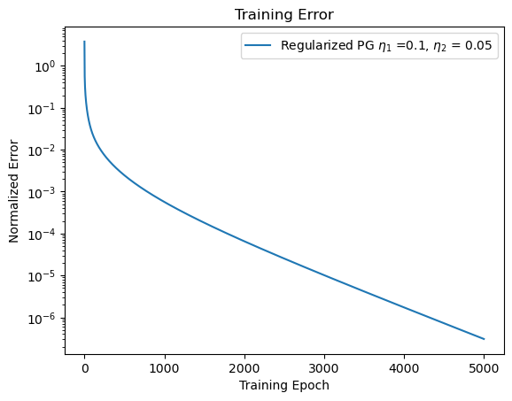
(a)

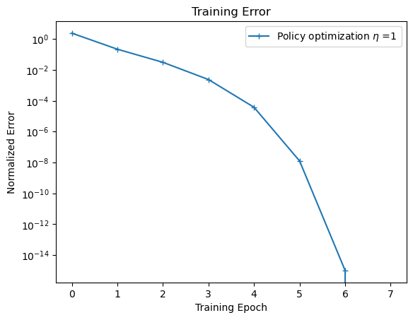
(b)

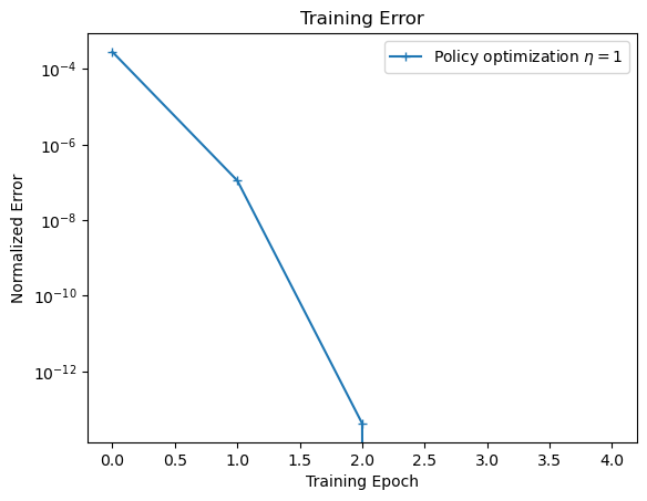
(c)

Figure 1: Performances of (1(a)) (RPG); (1(b)) (IPO); (1(c)) transfer learning using (IPO) with $(\overline{K}^{(0)},\overline{\Sigma}^{(0)})=(K^{*},\Sigma^{*})$ and state transitions $(\overline{A},\overline{B})$.

Performance measure.

We use the following normalized error to quantify the performance of a given policy ${K,\Sigma}$,

$$\text{ Normalized error }=\frac{C({K,\Sigma})-C\left({K}^{*},\Sigma^{*}\right)}{C\left({K}^{*},\Sigma^{*}\right)},$$

where ${K}^{*},\Sigma^{*}$ is the optimal policy defined in Theorem 2.1.

(Fast) Convergence.

Figure 1(a) shows the linear convergence of (RPG), and Figure 1(b) shows the superior convergence rate of (IPO). The normalized error falls below $10^{-14}$ within just 6 iterations, and from the third iteration, it enters a region of super-linear convergence. Figure 1(c) shows the result of applying transfer learning using (IPO) in a perturbed environment, when the optimal policy in Figure 1(a) and 1(b) serves as an initialization. Figure 1(c) shows that if the process commences within a super-linear convergence region, then the error falls below $10^{-12}$ in just 2 epochs.

8 Detailed Proofs

8.1 Proofs in Section 2

Proof.

(of Lemma 2.2). Let $\lambda$ be a Lagrangian multiplier to the constraint $\int_{\mathcal{A}}p(u)du=1.$ Consider

$$F(p,\lambda) =\int_{\mathcal{A}}\left(u^{\top}Mu+b^{\top}u+\tau\log p(u)\right)p(u)du+\lambda\left(\int_{\mathcal{A}}p(u)du-1\right)$$

$$=\int_{\mathcal{A}}\left(u^{\top}Mu+b^{\top}u+\tau\log p(u)+\lambda\right)p(u)du-\lambda$$

$$=\int_{\mathcal{A}}\mathcal{L}\left(u,p(u),\lambda\right)du-\lambda,$$

where $\mathcal{L}(u,v,\lambda):=(u^{\top}Mu+b^{\top}u)v+\tau v\log v+\lambda v.$ Since $\frac{\partial\mathcal{L}}{\partial{v}}=\lambda+u^{\top}Mu+b^{\top}u+\tau+\tau\log v,$ by setting $\frac{\partial\mathcal{L}}{\partial{v}}=0,$ we then get $v\propto e^{-\frac{1}{\tau}(u^{\top}Mu+b^{\top}u)}.$ Thus, the optimal solution $p^{*}$ is a multivariate Gaussian distribution with $\mathcal{N}\left(-\frac{1}{2}M^{-1}b,\frac{\tau}{2}M^{-1}\right)$.

8.2 Proofs in Section 3

8.2.1 Proof of Lemma 3.1

$\nabla_{\Sigma}C(K,\Sigma)$ in (18) can be checked by direct gradient calculation. To verify $\nabla_{K}C(K,\Sigma)$ in (18), first define $f:\mathcal{X}\times\mathbb{R}^{k\times n}\rightarrow\mathbb{R}$ by $f(y,K):=y^{\top}P_{K}y,\forall y\in\mathcal{X}$ and we aim to find the gradient of $f$ with respect to $K$. For any $y\in\mathcal{X},$ by the Riccati Equation for $P_{K}$ in (17) we have

$$f(y,K) =y^{\top}\left(\gamma(A-BK)^{\top}P_{K}(A-BK)+Q+K^{\top}RK\right)y$$

$$=\gamma f\left((A-BK)y,K\right)+y^{\top}\left(Q+K^{\top}RK\right)y.$$

$\nabla_{K}f((A-BK)y,K)$ has two terms: one with respect to the input $(A-BK)y$ and one with respect to $K$ in the subscript of $P_{K}$. This implies

$$\nabla_{K}f(y,K)=2\left(-\gamma B^{\top}P_{K}(A-BK)+RK\right)yy^{\top}+\gamma\nabla_{K}f(y^{\prime},K)|_{y^{\prime}=(A-BK)y}$$ (41)

$$=2\left(-\gamma B^{\top}P_{K}(A-BK)+RK\right)\sum_{i=0}^{\infty}\gamma^{i}(A-BK)^{i}yy^{\top}(A^{\top}-K^{\top}B^{\top})^{i}.$$

Since $C(K,\Sigma)=\mathbb{E}_{x_{0}\sim\mathcal{D}}[x_{0}P_{K}x_{0}]+q_{K,\Sigma}$ with $P_{K}$ and $q_{K,\Sigma}$ satisfying (17), then the gradient of $C(K,\Sigma)$ with respect to $K$ is

$$\nabla_{K}C(K,\Sigma)= \mathbb{E}[\nabla_{K}f(x_{0},K)]+\nabla_{K}q_{K,\Sigma}$$

$$\overset{(a)}{=} \mathbb{E}\Big{[}2\left(-\gamma B^{\top}P_{K}(A-BK)+RK\right)x_{0}x_{0}^{\top}+\gamma\nabla_{K}f(\hat{x}_{1},K)|_{\hat{x}_{1}=(A-BK)x_{0}}$$

$$+\sum_{t=0}\gamma^{t+1}\left(\nabla_{K}(\Sigma B^{\top}P_{K}B)+\nabla_{K}(w_{t}^{\top}P_{K}w_{t})\right)\Big{]}$$

$$\overset{(b)}{=} \mathbb{E}\Big{[}2\left(-\gamma B^{\top}P_{K}(A-BK)+RK\right)x_{0}x_{0}^{\top}+\gamma\nabla_{K}f({x}_{1},K)|_{{x}_{1}=A+Bu_{0}+w_{0}}$$

$$+\sum_{t=1}\gamma^{t+1}\left(\nabla_{K}(\Sigma B^{\top}P_{K}B)+\nabla_{K}(w_{t}^{\top}P_{K}w_{t})\right)\Big{]}$$

$$\overset{(c)}{=} 2\left(-\gamma B^{\top}P_{K}(A-BK)+RK\right)\mathbb{E}\left[\sum_{i=0}^{\infty}\gamma^{i}x_{i}x_{i}^{\top}\right],$$

where $(a)$ follows from applying (41) with $y=x_{0}$ and taking the gradient of $q_{K,\Sigma}$ in (17) with respect to $K$; $(b)$ follows from

$$\mathbb{E}_{x_{0},u_{0},w_{0}}[f(Ax_{0}+Bu_{0}+w_{0}),K]=\mathbb{E}_{x_{0},w_{0}}[f\left((A-BK)x_{0},K\right)+w_{0}^{\top}P_{K}w_{0}]+\Sigma B^{\top}P_{K}B.$$

Using recursion to get $(c)$. ∎

8.2.2 Proof of Lemma 3.2

For a given policy $\pi_{K,\Sigma}(\cdot|x)=\mathcal{N}(-Kx,\Sigma)$ with parameter $K$ and $\Sigma$, we define the state-action value function (also known as $Q$-function) $Q_{K,\Sigma}:\mathcal{X}\times\mathcal{A}\rightarrow\mathbb{R}$ as the cost of the policy starting with $x_{0}=x$, taking a fixed action $u_{0}=u$ and then proceeding with $\pi_{K,\Sigma}$. The $Q$-function is related to the value function $J_{K,\Sigma}$ defined in (2) as

$$Q_{K,\Sigma}(x,u)= x^{\top}Qx+u^{\top}Ru+\tau\pi_{K,\Sigma}(u|x)+\gamma\mathbb{E}\left[J_{K,\Sigma}(Ax+Bu+w)\right],$$ (42)

for any $(x,u)\in\mathcal{X}\times\mathcal{A}$. By definition of the $Q$-function, we also have the relationship:

$$\forall x\in\mathcal{X}:\quad J_{K,\Sigma}(x)=\mathbb{E}_{u\sim\pi(\cdot|x)}\left[Q_{K,\Sigma}(x,u)\right].$$ (43)

We also introduce the advantage function $A_{K,\Sigma}:\mathcal{X}\times\mathcal{A}\rightarrow\mathbb{R}$ of the policy $\pi$:

$$A_{K,\Sigma}(x,u)=Q_{K,\Sigma}(x,u)-J_{K,\Sigma}(x),$$ (44)

which reflects the gain one can harvest by executing control $u$ instead of following the policy $\pi_{K,\Sigma}$ in state $x$.

With the notations of the Q-function in (42) and the advantage function in (44), we first provide a convenient form for the difference of the cost functions with respect to two different policies in Lemma 8.1. This will be used in the proof of Lemma 3.2.

Lemma 8.1 (Cost difference).

Suppose policies $\pi$ and $\pi^{\prime}$ are in form of (14) with parameters $(K^{\prime},\Sigma^{\prime})$ and $(K,\Sigma).$ Let $\{x_{t}^{\prime}\}_{t=0}^{\infty}$ and $\{u_{t}^{\prime}\}_{t=0}^{\infty}$ be state and action sequences generated by $\pi^{\prime}$ with noise sequence $\{w_{t}^{\prime}\}_{t=0}^{\infty}$ (i.i.d with mean $0$ and covariance $W$), i.e., $x_{t+1}^{\prime}=Ax_{t}^{\prime}+Bu_{t}^{\prime}+w_{t}^{\prime}$. Then for any $x\in\mathcal{X},$

$$J_{K^{\prime},\Sigma^{\prime}}(x)-J_{K,\Sigma}(x)=\mathbb{E}_{\pi^{\prime}}\left[\left.\sum_{t=0}^{\infty}\gamma^{t}A_{K,\Sigma}(x_{t}^{\prime},u_{t}^{\prime})\right|x_{0}^{\prime}=x\right],$$ (45)

where the expectation is taken over $u_{t}^{\prime}\sim\pi^{\prime}(\cdot|x_{t}^{\prime})$ and $w_{t}$ for all $t=0,1,2,\cdots$.

The expected advantage for any $x\in\mathcal{X}$ by taking expectation over $u\sim\pi^{\prime}(\cdot|x)$ is:

$$\mathbb{E}_{\pi^{\prime}}\left[A_{K,\Sigma}(x,u)\right]=x^{\top}(K^{\prime}-K)^{\top}(R+\gamma B^{\top}P_{K}B)(K^{\prime}-K)x$$ (46)

$$\quad+2x^{\top}(K^{\prime}-K)^{\top}\left[(R+\gamma B^{\top}P_{K}B)K-\gamma B^{\top}P_{K}A\right]x+(1-\gamma)(f_{K}(\Sigma)-f_{K}(\Sigma^{\prime})).$$

Proof.

(of Lemma 8.1). Let $\{c_{t}^{\prime}\}_{t=0}^{\infty}$ be the cost sequences generated by $\pi^{\prime},$ i.e., $c_{t}^{\prime}=x_{t}^{\prime\top}Qx_{t}^{\prime}+u_{t}^{\prime\top}Ru_{t}^{\prime}+\tau\log\pi^{\prime}(u_{t}^{\prime}|x_{t}^{\prime}),$ and $J_{K^{\prime},\Sigma^{\prime}}(x)=\mathbb{E}_{\pi^{\prime}}\left[\sum_{t=0}^{\infty}\gamma^{t}c_{t}^{\prime}\right]$. Then we have

$$J_{K^{\prime},\Sigma^{\prime}}(x)-J_{K,\Sigma}(x)=\mathbb{E}_{\pi^{\prime}}\left[\sum_{t=0}^{\infty}\gamma^{t}c_{t}^{\prime}\right]-J_{K,\Sigma}(x)$$

$$= \mathbb{E}_{\pi^{\prime}}\left[\sum_{t=0}^{\infty}\gamma^{t}\left(c_{t}^{\prime}-J_{K,\Sigma}(x_{t}^{\prime})+J_{K,\Sigma}(x_{t}^{\prime})\right)\right]-J_{K,\Sigma}(x)$$

$$\overset{(a)}{=} \mathbb{E}_{\pi^{\prime}}\left[\sum_{t=0}^{\infty}\gamma^{t}\left(c_{t}^{\prime}-J_{K,\Sigma}(x_{t}^{\prime})\right)+\sum_{t=1}^{\infty}\gamma^{t}J_{K,\Sigma}(x_{t}^{\prime})\right]=\mathbb{E}_{\pi^{\prime}}\left[\sum_{t=0}^{\infty}\gamma^{t}\left(c_{t}^{\prime}+\gamma J_{K,\Sigma}(x_{t+1}^{\prime})-J_{K,\Sigma}(x_{t}^{\prime})\right)\right]$$

$$= \mathbb{E}_{\pi^{\prime}}\left[\sum_{t=0}^{\infty}\gamma^{t}\left(x_{t}^{\prime\top}Qx_{t}^{\prime}+u_{t}^{\prime\top}Ru_{t}^{\prime}+\tau\log\pi^{\prime}(u_{t}^{\prime}|x_{t}^{\prime})+\gamma J_{K,\Sigma}(x_{t+1}^{\prime})-J_{K,\Sigma}(x_{t}^{\prime})\right)\right],$$

where $(a)$ follows from $x_{0}^{\prime}=x$. By (42) and (44), we can continue the above calculations by

$$J_{K^{\prime},\Sigma^{\prime}}(x)-J_{K,\Sigma}(x) =\mathbb{E}_{\pi^{\prime}}\left[\sum_{t=0}^{\infty}\gamma^{t}\left(Q_{K,\Sigma}(x_{t}^{\prime},u_{t}^{\prime})-J_{K,\Sigma}(x_{t}^{\prime})\right)\right]=\mathbb{E}_{\pi^{\prime}}\left[\sum_{t=0}^{\infty}\gamma^{t}A_{K,\Sigma}(x_{t}^{\prime},u_{t}^{\prime})\right].$$

To derive the expectation of the advantage function, for any $x$ in $\mathcal{X}$, take expectation over $u\sim\pi^{\prime}(\cdot|x):=\mathcal{N}(-K^{\prime}x,\Sigma^{\prime})$ to get:

$$\mathbb{E}_{\pi^{\prime}} \left[A_{K,\Sigma}(x,u)\right]=\mathbb{E}_{\pi^{\prime}}[Q_{K,\Sigma}(x,u)]-J_{K,\Sigma}(x)$$

$$= x^{\top}(Q+K^{\prime\top}RK^{\prime})x+\text{Tr}(\Sigma^{\prime}R)-\frac{\tau}{2}\left(k+\log\left((2\pi)^{k}\operatorname{det}\Sigma^{\prime}\right)\right)$$

$$+\gamma\mathbb{E}\left[(Ax+Bu+w)^{\top}P_{K}(Ax+Bu+w)+q_{K,\Sigma}\right]-x^{\top}P_{K}x-q_{K,\Sigma}$$

$$= x^{\top}(Q+K^{\prime\top}RK^{\prime})x+\text{Tr}(\Sigma^{\prime}R)-\frac{\tau}{2}\left(k+\log\left((2\pi)^{k}\operatorname{det}\Sigma^{\prime}\right)\right)-x^{\top}P_{K}x-(1-\gamma)q_{K,\Sigma}$$

$$+\gamma\left[x^{\top}(A-BK^{\prime})^{\top}P_{K}(A-BK^{\prime})x+\text{Tr}(\Sigma^{\prime}B^{\top}P_{K}B)+\text{Tr}(WP_{K})\right].$$

Plug (17) into the above equation, then use (16) and write $K^{\prime}=K+K^{\prime}-K$ to get

$$\mathbb{E}_{\pi^{\prime}} \left[A_{K,\Sigma}(x,u)\right]$$

$$= (1-\gamma)(f_{K}(\Sigma)-f_{K}(\Sigma^{\prime}))+x^{\top}\left(Q+(K+K^{\prime}-K)^{\top}R(K+K^{\prime}-K)\right)x$$

$$+\gamma x^{\top}(A-BK-B(K^{\prime}-K))^{\top}P_{K}(A-BK-B(K^{\prime}-K))x-x^{\top}P_{K}x$$

$$= (1-\gamma)(f_{K}(\Sigma)-f_{K}(\Sigma^{\prime}))+x^{\top}\left(Q+K^{\top}RK+\gamma(A-BK)^{\top}P_{K}(A-BK)\right)x$$

$$+2x^{\top}(K^{\prime}-K)^{\top}\left[(R+\gamma B^{\top}P_{K}B)K-\gamma B^{\top}P_{K}A\right]x$$

$$+x^{\top}(K^{\prime}-K)^{\top}(R+\gamma B^{\top}P_{K}B)(K^{\prime}-K)x-x^{\top}P_{K}x.$$

Plugging (17) finishes the proof to verify (46). ∎

Proof.

(of Lemma 3.2). By Lemma 8.1, for any $\pi$ and $\pi^{\prime}$ in form of (14) with parameter $(K,\Sigma)$ and $(K^{\prime},\Sigma^{\prime})$ respectively, and for any $x\in\mathcal{X}$,

$$\mathbb{E}_{\pi^{\prime}}[A_{K,\Sigma} (x,u)]=(1-\gamma)(f_{K}(\Sigma)-f_{K}(\Sigma^{\prime}))-\operatorname{Tr}\left(xx^{\top}E_{K}^{\top}\left(R+\gamma B^{\top}P_{K}B\right)^{-1}E_{K}\right)$$

$$\quad+\operatorname{Tr}\Bigl{[}xx^{\top}\left(K^{\prime}-K+\left(R+\gamma B^{\top}P_{K}B\right)^{-1}E_{K}\right)^{\top}\left(R+\gamma B^{\top}P_{K}B\right)$$

$$\quad\quad\cdot\left(K^{\prime}-K+(R+\gamma B^{\top}P_{K}B)^{-1}E_{K}\right)\Bigr{]}$$

$$\geq-\operatorname{Tr}\left(xx^{\top}E_{K}^{\top}\left(R+\gamma B^{\top}P_{K}B\right)^{-1}E_{K}\right)+(1-\gamma)\left(f_{K}\left(\Sigma\right)-f_{K}\left(\Sigma^{\prime}\right)\right),$$ (47)

with equality when $K-(R+\gamma B^{\top}P_{K}B)^{-1}E_{K}=K^{\prime}$ holds. Let $\{x_{t}^{*}\}_{t=0}^{\infty}$ and $\{u_{t}^{*}\}_{t=0}^{\infty}$ be the state and control sequences generated under $\pi^{*}(\cdot|x)=\mathcal{N}(-K^{*}x,\Sigma^{*})$ with noise sequence $\{w_{t}^{*}\}_{t=0}^{\infty}$ with mean $0$ and covariance $W$. Apply Lemma 8.1 and (47) with $\pi$ and $\pi^{*}$ to get:

$$C(K,\Sigma)-C(K^{*},\Sigma^{*})=-\mathbb{E}_{\pi^{*}}\Bigg{[}\sum_{t=0}^{\infty}\gamma^{t}A_{K,\Sigma}(x_{t}^{*},u_{t}^{*})\Bigg{]}$$

$$\leq\operatorname{Tr}\left(S_{K^{*},\Sigma^{*}}E_{K}^{\top}\left(R+\gamma B^{\top}P_{K}B\right)^{-1}E_{K}\right)+f_{K}(\Sigma^{*})-f_{K}(\Sigma),$$ (48)

where $f_{K}$ is defined in (16). To analyze the first term in (48), note that

$$\operatorname{Tr}\left(S_{K^{*},\Sigma^{*}}E_{K}^{\top}\left(R+\gamma B^{\top}P_{K}B\right)^{-1}E_{K}\right)\leq\frac{\|S_{K^{*},\Sigma^{*}}\|}{\sigma_{\min}(R)}\operatorname{Tr}(E_{K}^{\top}E_{K})$$ (49)

$$\leq\frac{\|S_{K^{*},\Sigma^{*}}\|}{\mu^{2}\sigma_{\min}(R)}\operatorname{Tr}\left(S_{K,\Sigma}E_{K}^{\top}E_{K}S_{K,\Sigma}\right)=\frac{\|S_{K^{*},\Sigma^{*}}\|}{4\mu^{2}\sigma_{\min}(R)}\operatorname{Tr}(\nabla_{K}^{\top}C(K,\Sigma)\nabla_{K}C(K,\Sigma)),$$

where the last equation follows from (18).

To analyze the second terms in (48), note that $f_{K}$ is a concave function, thus we can find its maximizer $\Sigma_{K}^{*}$ by taking the gradient of $f_{K}$ and setting it to $0$, i.e., $\Sigma_{K}^{*}=\frac{\tau}{2}(R+\gamma B^{\top}P_{K}B)^{-1}.$ Thus,

$$f_{K}(\Sigma^{*})-f_{K}(\Sigma)\leq f_{K}(\Sigma_{K}^{*})-f_{K}(\Sigma)\overset{(a)}{\leq}\operatorname{Tr}\left(\nabla f_{K}(\Sigma)^{\top}(\Sigma_{K}^{*}-\Sigma)\right)$$ (50)

$$=\operatorname{Tr}\left(\nabla_{\Sigma}C(K,\Sigma)\cdot(R+\gamma B^{\top}P_{K}B)^{-1}\left((R+\gamma B^{\top}P_{K}B)-\frac{\tau}{2}\Sigma^{-1}\right)\Sigma\right)$$

$$\overset{(b)}{\leq}(1-\gamma)\cdot\|(R+\gamma B^{\top}P_{K}B)^{-1}\|\cdot\|\nabla_{\Sigma}C(K,\Sigma)\|_{F}^{2}\leq\frac{(1-\gamma)\|\nabla_{\Sigma}C(K,\Sigma)\|_{F}^{2}}{\sigma_{\min}(R)},$$

where $(a)$ follows from the first order concavity condition for $f_{K}$ and $(b)$ is from $0\prec\Sigma\preceq I.$

For the lower bound, consider $K^{\prime}=K-(R+\gamma B^{\top}P_{K}B)^{-1}E_{K}$ and $\Sigma^{\prime}=\Sigma$ where equality holds in (47). Let $\{x_{t}^{\prime}\}_{t=0}^{\infty}$, $\{u_{t}^{\prime}\}_{t=0}^{\infty}$ be the sequence generated with $K^{\prime},\Sigma^{\prime}$. By $C(K^{*},\Sigma^{*})\leq C(K^{\prime},\Sigma^{\prime}),$ we have

$$C(K,\Sigma)-C(K^{*},\Sigma^{*})\geq C(K,\Sigma)-C(K^{\prime},\Sigma^{\prime})=-\mathbb{E}\left[\sum_{t=0}^{\infty}\gamma^{t}A_{K,\Sigma}(x_{t}^{\prime},u_{t}^{\prime})\right]$$

$$=\operatorname{Tr}\left(S_{K^{\prime},\Sigma^{\prime}}E_{K}^{\top}\left(R+\gamma B^{\top}P_{K}B\right)^{-1}E_{K}\right)\geq\frac{\mu}{\|R+\gamma B^{\top}P_{K}B\|}\operatorname{Tr}(E_{K}^{\top}E_{K}).$$

∎

8.2.3 Proof of Lemma 3.3

Lemma 8.2 shows that the cost objective is smooth in $\Sigma$ when utilizing entropy regularization, given that $\Sigma$ is bounded.

Lemma 8.2 (Smoothness of $f_{K}$ (16)).

Let $K\in\mathbb{R}^{k\times n}$ be given and let $f_{K}$ be defined in (16). Fix $0<a\leq 1$. For any symmetric positive definite matrices $X\in\mathbb{R}^{k\times k}$ and $Y\in\mathbb{R}^{k\times k}$ satisfying $aI\preceq X\preceq I$ and $aI\preceq Y\preceq I$, the following inequality holds

$$\left|f_{K}(X)-f_{K}(Y)+\operatorname{Tr}\left(\nabla f_{K}(X)^{\top}(Y-X)\right)\right|\leq M_{a}\operatorname{Tr}\left((X^{-1}Y-I)^{2}\right),$$

where $M_{a}\in\mathbb{R}$ is defined in Lemma 3.3, and $M_{a}\geq\frac{\tau}{4(1-\gamma)}$.

Proof.

(of Lemma 8.2). Fix symmetric positive definite matrices $X$ and $Y$ satisfying $aI\preceq X\preceq I$ and $aI\preceq Y\preceq I$. Then $f_{K}$ being concave implies $f_{K}(X)-f_{K}(Y)+\operatorname{Tr}\left(\nabla f_{K}(X)^{\top}(Y-X)\right)\geq 0.$ To find an upper bound, observe that

$$f_{K}(X)-f_{K}(Y)+\operatorname{Tr}\left(\nabla f_{K}(X)^{\top}(Y-X)\right)$$ (51)

$$= \frac{\tau}{2(1-\gamma)}\left(\log\operatorname{det}(X)-\log\operatorname{det}(Y)+\operatorname{Tr}\left(X^{-1}(Y-X)\right)\right).$$

Since $X\succ 0$ and $Y\succ 0,$ then all eigenvalues of $X^{-1}Y$ are real and positive and $\sigma_{\min}(X^{-1}Y)\geq\sigma_{\min}(X^{-1})\sigma_{\min}(Y)\geq a.$

Now let us show that there exists a constant $m>0$ (independent of $K$) such that for any $Z\in\mathbb{R}^{k\times k}$ with real positive eigenvalues $a\leq z_{1}\leq\cdots\leq z_{k}$, the following holds:

$$-\log(\det(Z))+\operatorname{Tr}(Z-I)\leq m\operatorname{Tr}((Z-I)^{2}).$$ (52)

Note that (52) is equivalent to $\sum_{i=1}^{k}-\log(z_{i})+z_{i}-1\leq m\sum_{i=1}^{k}(z_{i}-1)^{2}.$ With elementary algebra, one can verify that when $m:={(-\log\left(a\right)+a-1)}\cdot{\left(a-1\right)^{-2}},$ it holds that $-\log(z)+z-1\leq m(z-1)^{2}$ for all $z\geq a$ and such an $m$ satisfies $m\geq\frac{1}{2}$. Therefore, (52) holds. Combining (51) and (52) with $Z=X^{-1}Y$, we see

$$f_{K}(X)-f_{K}(Y)+\operatorname{Tr}\left(\nabla f_{K}(X)^{\top}(Y-X)\right)\leq\frac{\tau m}{2(1-\gamma)}\operatorname{Tr}\left((X^{-1}Y-I)^{2}\right).$$

∎

Proof.

(of Lemma 3.3). The first equality immediately results from Lemma 8.1, by taking an expectation with respect to $x$ in (46). The last inequality follows directly from Lemma 8.2. ∎

8.3 Proofs in Section 4

8.3.1 Proofs of Lemma 4.3

To ease the exposition, let $\eta$ denote $\eta_{2}$. The proof is composed of two steps. First, one can show

$$aI\preceq\Sigma-\frac{\eta}{1-\gamma}\left(R-\frac{\tau}{2}\Sigma^{-1}+\gamma B^{\top}P_{K}B\right)\preceq I.$$ (53)

Let $g:\mathbb{R}^{+}\rightarrow\mathbb{R}$ be a function such that $g(x)=x+\frac{{\eta}\tau}{2(1-\gamma)x}.$ Thus, $g$ monotonically increases on $\left[\sqrt{\frac{{\eta}\tau}{2(1-\gamma)}},\infty\right)$. Since $\sqrt{\frac{{\eta}\tau}{2(1-\gamma)}}\leq a\leq\frac{\sigma_{\min}(R)}{\|R+\gamma B^{\top}P_{K}B\|}\leq 1,$ then

$$\Sigma+\frac{{\eta}\tau}{2(1-\gamma)}\Sigma^{-1}-\frac{\eta}{1-\gamma}(R+\gamma B^{\top}P_{K}B)\succeq\left(a+\frac{{\eta}\tau}{2(1-\gamma)a}\right)I-\frac{\eta}{1-\gamma}(R+\gamma B^{\top}P_{K}B)$$

$$\succeq\left(a+\frac{\eta}{1-\gamma}\|{R}+\gamma B^{\top}P_{K}B\|\right)I-\frac{\eta}{1-\gamma}(R+\gamma B^{\top}P_{K}B)\succeq aI,$$

and

$$\Sigma+\frac{{\eta}\tau}{2(1-\gamma)}\Sigma^{-1}-\frac{\eta}{1-\gamma}(R+\gamma B^{\top}P_{K}B)\preceq\left(1+\frac{{\eta}\tau}{2(1-\gamma)}\right)I-\frac{\eta}{1-\gamma}(R+\gamma B^{\top}P_{K}B)$$

$$\preceq\left(1+\frac{\eta}{1-\gamma}\sigma_{\min}(R)\right)I-\frac{\eta}{1-\gamma}(R+\gamma B^{\top}P_{K}B)\preceq I,$$

hence (53).

Second, one can show $aI\preceq\Sigma^{\prime}\preceq I:$ observe that (53) is equivalent to

$$aI-\Sigma\preceq-\frac{\eta}{1-\gamma}(R+\gamma B^{\top}P_{K}B-\frac{\tau}{2}\Sigma^{-1})\preceq I-\Sigma.$$

Then by multiplying $\Sigma$ to both sides then adding a $\Sigma$ to each term, we have

$$a\Sigma^{2}-\Sigma^{3}+\Sigma\preceq\Sigma-\frac{\eta}{1-\gamma}\Sigma(R+\gamma B^{\top}P_{K}B-\frac{\tau}{2}\Sigma^{-1})\Sigma\preceq\Sigma^{2}-\Sigma^{3}+\Sigma.$$

With $aI-\Sigma\preceq 0$, $I-\Sigma\succeq 0$ and $\Sigma\preceq I$, it holds that $aI-\Sigma\preceq(aI-\Sigma)\Sigma^{2},$ and $I-\Sigma\succeq(I-\Sigma)\Sigma^{2}.$ This implies $aI\preceq a\Sigma^{2}-\Sigma^{3}+\Sigma\preceq\Sigma^{\prime}\preceq\Sigma^{2}-\Sigma^{3}+\Sigma\preceq I.$

8.3.2 Proof of Lemma 4.4

For ease of exposition, write $S=S_{K,\Sigma},$ $S^{\prime}=S_{K^{\prime},\Sigma^{\prime}}$, and $S^{*}=S_{K^{*},\Sigma^{*}}$. Let $M_{a}$ be defined in the same way as in Lemma 3.3. Let $f_{K}$ be defined as (16). Then Lemma 3.3 implies

$$C(K^{\prime},\Sigma^{\prime})-C(K,\Sigma) =\operatorname{Tr}\left(S^{\prime}(K^{\prime}-K)^{\top}(R+\gamma B^{\top}P_{K}B)(K^{\prime}-K)\right)$$ (54)

$$\quad+2\operatorname{Tr}\left(S^{\prime}(K^{\prime}-K)^{\top}E_{K}\right)+f_{K}(\Sigma)-f_{K}(\Sigma^{\prime}).$$

By (RPG),

$$\operatorname{Tr}\left(S^{\prime}(K^{\prime}-K)^{\top}(R+\gamma B^{\top}P_{K}B)(K^{\prime}-K)\right)+2\operatorname{Tr}\left(S^{\prime}(K^{\prime}-K)^{\top}E_{K}\right)$$ (55)

$$\leq 4\eta_{1}^{2}\|R+\gamma B^{\top}P_{K}B\|\operatorname{Tr}\left(S^{\prime}E_{K}^{\top}E_{K}\right)-4\eta_{1}\operatorname{Tr}\left(S^{\prime}E_{K}^{\top}E_{K}\right)\overset{(a)}{\leq}-2\eta_{1}\operatorname{Tr}\left(S^{\prime}E_{K}^{\top}E_{K}\right)$$

$$\leq -2\eta_{1}\mu\operatorname{Tr}\left(E_{K}^{\top}E_{K}\right)\overset{(b)}{\leq}-2\eta_{1}\mu\frac{\sigma_{\min}(R)}{\|S^{*}\|}\operatorname{Tr}\left(S_{K^{*},\Sigma^{*}}E_{K}^{\top}\left(R+\gamma B^{\top}P_{K}B\right)^{-1}E_{K}\right),$$

where (a) follows from $\eta_{1}\leq\frac{1}{2\|R+\gamma B^{\top}P_{K}B\|}$ and (b) follows from (49).

By Lemma 4.3, $aI\preceq\Sigma^{\prime}\preceq I.$ Using Lemma 8.2, one can derive the following inequality:

$$f_{K}(\Sigma)-f_{K}(\Sigma^{\prime})$$

$$\leq\frac{1}{1-\gamma}\operatorname{Tr}\left(\left(R+\gamma B^{\top}P_{K}B-\frac{\tau}{2}\Sigma^{-1}\right)(\Sigma^{\prime}-\Sigma)\right)+M_{a}\operatorname{Tr}\left((\Sigma^{-1}\Sigma^{\prime}-I)^{2}\right)$$

$$=-\frac{\eta_{2}}{(1-\gamma)^{2}}\operatorname{Tr}\left(\left(R+\gamma B^{\top}P_{K}B-\frac{\tau}{2}\Sigma^{-1}\right)\Sigma\left(R+\gamma B^{\top}P_{K}B-\frac{\tau}{2}\Sigma^{-1}\right)\Sigma\right)$$

$$\quad\quad\quad\quad+\frac{\eta^{2}_{2}}{(1-\gamma)^{2}}M_{a}\operatorname{Tr}\left(\left((R+\gamma B^{\top}P_{K}B)\Sigma-\frac{\tau}{2}I\right)^{2}\right)$$

$$\overset{(b)}{\leq} -\frac{\eta_{2}}{2(1-\gamma)^{2}}\operatorname{Tr}\left(\left((R+\gamma B^{\top}P_{K}B)\Sigma-\frac{\tau}{2}I\right)^{2}\right).$$

Here $(b)$ follows from the inequality

$$\eta_{2}=\frac{2(1-\gamma)a^{2}}{\tau}\leq\frac{2(1-\gamma)}{\tau}\left(\frac{\tau}{2\|R+\gamma B^{\top}P_{K}B\|}\right)^{2}\overset{(c)}{\leq}\frac{2(1-\gamma)}{\tau}\overset{(d)}{\leq}\frac{1}{2M_{a}}.$$

$(c)$ is obtained from the fact that $\tau\leq 2\sigma_{\min}(R)\leq 2\|R+\gamma B^{\top}P_{K}B\|$, and $(d)$ follows from Lemma 8.2. Meanwhile, observe from (50) that

$$f_{K}(\Sigma^{*})-f_{K}(\Sigma)$$

$$\leq\frac{1}{(1-\gamma)}\operatorname{Tr}\left(\left((R+\gamma B^{\top}P_{K}B)\Sigma-\frac{\tau}{2}I\right)\Sigma^{-1}(R+\gamma B^{\top}P_{K}B)^{-1}\left((R+\gamma B^{\top}P_{K}B)\Sigma-\frac{\tau}{2}I\right)\right)$$

$$\leq\frac{1}{(1-\gamma)a\sigma_{\min}(R)}\operatorname{Tr}\left(((R+\gamma B^{\top}P_{K}B)\Sigma-\frac{\tau}{2}I)^{2}\right),$$

while implies

$$f_{K}(\Sigma)-f_{K}(\Sigma^{\prime}) \leq-\frac{\eta_{2}a\sigma_{\min}(R)}{2(1-\gamma)}\left(f_{K}(\Sigma)-f_{K}(\Sigma^{*})\right).$$ (56)

Finally, with $\zeta=\min\left\{\frac{2\mu\eta_{1}\sigma_{\min}(R)}{\|S^{*}\|},\frac{\eta_{2}a\sigma_{\min}(R)}{2(1-\gamma)}\right\}$, plug (55) and (56) in (54) to get

$$C(K^{\prime},\Sigma^{\prime})-C(K,\Sigma)$$

$$\leq-2\eta_{1}\mu\frac{\sigma_{\min}(R)}{\|S^{*}\|}\operatorname{Tr}\left(S_{K^{*},\Sigma^{*}}E_{K}^{\top}\left(R+\gamma B^{\top}P_{K}B\right)^{-1}E_{K}\right)-\frac{\eta_{2}a\sigma_{\min}(R)}{2(1-\gamma)}\left(f_{K}(\Sigma)-f_{K}(\Sigma^{*})\right)$$

$$\leq-\zeta\left(\operatorname{Tr}\left(S_{K^{*},\Sigma^{*}}E_{K}^{\top}\left(R+\gamma B^{\top}P_{K}B\right)^{-1}E_{K}\right)+f_{K}(\Sigma)-f_{K}(\Sigma^{*})\right)$$

$$\leq-\zeta(C(K,\Sigma)-C(K^{*},\Sigma^{*}))$$

where the last inequality follows from (48). Adding $C(K,\Sigma)-C(K^{*},\Sigma^{*})$ to both sides of the above inequality finishes the proof.

8.3.3 Proof of Lemma 4.5

By (15) and (17),

$$C(K,\Sigma)= \mathbb{E}_{x_{0}\sim\mathcal{D}}\left[x_{0}^{\top}P_{K}x_{0}\right]+\frac{\gamma}{1-\gamma}\operatorname{Tr}(WP_{K})$$

$$+\frac{1}{1-\gamma}\operatorname{Tr}\left(\Sigma(R+\gamma B^{\top}P_{K}B)\right)-\frac{\tau}{2(1-\gamma)}(k+\log((2\pi)^{k}\operatorname{det}\Sigma)).$$

Note that

$$\frac{1}{1-\gamma}\operatorname{Tr}\left(\Sigma(R+\gamma B^{\top}P_{K}B)\right)-\frac{\tau}{2(1-\gamma)}(k+\log((2\pi)^{k}\operatorname{det}\Sigma))$$

$$\geq\frac{1}{1-\gamma}\left(\sigma_{\min}(R)\operatorname{Tr}(\Sigma)-\frac{\tau}{2}\left(k+k\log(2\pi)\right)-\frac{\tau}{2}\log\operatorname{det}\Sigma\right)$$

$$\overset{(a)}{\geq}\frac{1}{1-\gamma}\left(\frac{\tau k}{2}-\frac{\tau}{2}\left(k+k\log(2\pi)\right)-\frac{\tau k}{2}\log(\frac{\tau}{2\sigma_{\min}(R)})\right)$$

$$=\frac{\tau k}{2(1-\gamma)}\log(\frac{\sigma_{\min}(R)}{\pi\tau})=:M_{\tau},$$

where $(a)$ follows from the fact that $\sigma_{\min}(R)\operatorname{Tr}(\Sigma)-\frac{\tau}{2}\left(k+k\log(2\pi)-\frac{\tau}{2}\log\operatorname{det}\Sigma\right)$ is a convex function with respect to $\Sigma$ with minimizer $\frac{\tau}{2\sigma_{\min}(R)}I.$ Thus,

$$C(K,\Sigma) \geq\mathbb{E}_{x_{0}\sim\mathcal{D}}\left[x_{0}^{\top}P_{K}x_{0}\right]+\frac{\gamma}{1-\gamma}\operatorname{Tr}(WP_{K})+M_{\tau}\geq\left(\mu+\frac{\gamma}{1-\gamma}\sigma_{\min}(W)\right)\|P_{K}\|+M_{\tau}.$$

8.4 Proofs in Section 5

8.4.1 Proof of Lemma 5.2

Let $K,\Sigma$ fixed and let $f_{K}$ be defined in (16). Observe that $\Sigma^{\prime}$ defined in (25) is the maximizer of $f_{K}$. Then by Lemma 3.3,

$$C( K^{\prime},\Sigma^{\prime})-C(K,\Sigma)=-\operatorname{Tr}\left(S_{K^{\prime},\Sigma^{\prime}}E_{K}^{\top}(R+\gamma B^{\top}P_{K}B)^{-1}E_{K}\right)-f_{K}(\Sigma^{\prime})+f_{K}(\Sigma)$$

$$\overset{(a)}{\leq} -\frac{\mu}{\|S_{K^{*},\Sigma^{*}}\|}\operatorname{Tr}\left(S_{K^{*},\Sigma^{*}}E_{K}^{\top}(R+\gamma B^{\top}P_{K}B)^{-1}E_{K}\right)-\frac{\mu}{\|S_{K^{*},\Sigma^{*}}\|}(f_{K}(\Sigma^{\prime})-f_{K}(\Sigma))$$

$$\overset{(b)}{\leq} -\frac{\mu}{\|S_{K^{*},\Sigma^{*}}\|}\Bigg{(}\operatorname{Tr}\left(S_{K^{*},\Sigma^{*}}E_{K}^{\top}(R+\gamma B^{\top}P_{K}B)^{-1}E_{K}\right)+f_{K}(\Sigma^{*})-f_{K}(\Sigma)\Bigg{)},$$

where $(a)$ follows the fact that $f_{K}(\Sigma^{\prime})-f_{K}(\Sigma)\geq 0$ and $\frac{\mu}{\|S_{K^{*},\Sigma^{*}}\|}\leq 1$; $(b)$ follows from fact that $f_{K}(\Sigma^{\prime})\geq f_{K}(\Sigma^{*}).$ Finally, apply (48) to get

$$C(K^{\prime},\Sigma^{\prime})-C(K,\Sigma)\leq -\frac{\mu}{\|S_{K^{*},\Sigma^{*}}\|}\left(C(K,\Sigma)-C(K^{*},\Sigma^{*})\right).$$

Adding $C(K,\Sigma)-C(K^{*},\Sigma^{*})$ to both sides of the above inequality finishes the proof.

8.4.2 Proof of Lemma 5.4

Let $K^{\prime}$ denote $K^{(t+1)}$, $K$ denote $K^{(t)}$ and $S^{\prime}$ denote $S^{(t+1)}$. Apply Lemma 3.3 with $f_{K}$ defined in (16) to get

$$C(K^{\prime},\Sigma^{\prime})-C(K,\Sigma)$$

$$= -\operatorname{Tr}\left(S^{*}E_{K}^{\top}(R+\gamma B^{\top}P_{K}B)^{-1}E_{K}\right)-\operatorname{Tr}\left((S^{\prime}-S^{*})E_{K}^{\top}(R+\gamma B^{\top}P_{K}B)^{-1}E_{K}\right)$$

$$+f_{K}(\Sigma)-f_{K}(\Sigma^{\prime})$$

$$\overset{(a)}{\leq} \left(-1+\|(S^{\prime}-S^{*})S^{*-1}\|\right)\left(\operatorname{Tr}\left(S^{*}E_{K}^{\top}(R+\gamma B^{\top}P_{K}B)^{-1}E_{K}\right)+f_{K}(\Sigma^{*})-f_{K}(\Sigma)\right),$$

where $(a)$ follows from the assumption $\|S^{\prime}-S^{*}\|\leq\sigma_{\min}(S^{*})$ which implies $-1+\left\|(S^{\prime}-S^{*})S^{*-1}\right\|\in[-1,0]$ and the fact $\Sigma^{\prime}$ is the maximizer of $f_{K}.$ Finally, apply (48) to get

$$C(K^{\prime},\Sigma^{\prime})-C(K,\Sigma) \leq\left(-1+\left\|(S^{\prime}-S^{*})S^{*-1}\right\|\right)\left(C(K,\Sigma)-C(K^{*},\Sigma^{*})\right)$$

$$\leq\left(-1+\frac{\left\|S^{\prime}-S^{*}\right\|}{\sigma_{\min}(S^{*})}\right)\left(C(K,\Sigma)-C(K^{*},\Sigma^{*})\right).$$

Adding $C(K,\Sigma)-C(K^{*},\Sigma^{*})$ to both sides of the above inequality finishes the proof.

8.4.3 Proof of Lemma 5.5

This section conducts a perturbation analysis on $S_{K,\Sigma}$ and aims to prove Lemma 5.5, which bounds $\|S_{K_{1},\Sigma_{1}}-S_{K_{2},\Sigma_{2}}\|$ by $\left\|K_{1}-K_{2}\right\|$ and $\|\Sigma_{1}-\Sigma_{2}\|$.

The proof of Lemma 5.5 proceeds with a few technical lemmas. First, define the linear operators on symmetric matrices. For symmetric matrix $X\in\mathbb{R}^{n\times n}$, we set

$$\mathcal{F}_{K}(X) :=(A-BK)X(A-BK)^{\top},\quad\mathcal{G}^{K}_{t}(X):=(A-BK)^{t}X(A-BK)^{\top t}$$ (57)

$$\mathcal{T}_{K}(X) :=\sum_{t=0}^{\infty}\gamma^{t}(A-BK)^{t}X(A-BK)^{\top t}=\sum_{t=0}^{\infty}\gamma^{t}\mathcal{G}^{K}_{t}(X).$$

Note that when $\|A-BK\|<\frac{1}{\sqrt{\gamma}}$, we have

$$\mathcal{T}_{K}=(I-\gamma\mathcal{F}_{K})^{-1}.$$ (58)

We also define the induced norm for these operators as $\|T\|:=\sup_{X}\frac{\|T(X)\|}{\|X\|},$ where $T=\mathcal{F}_{K},\mathcal{G}_{t}^{{K}},\mathcal{T}_{{K}}$ and the supremum is over all symmetric matrix $X\in\mathbb{R}^{n\times n}$ with non-zero spectral norm.

Lemma 8.3.

For any $K\in\mathbb{R}^{k\times n}$ and any symmetric $\Sigma\in\mathbb{R}^{n\times n}$,

$$S_{K,\Sigma}=\mathcal{T}_{K}(\mathbb{E}[x_{0}x_{0}^{\top}])+\sum_{t=0}^{\infty}\gamma^{t}\sum_{s=1}^{t}\mathcal{G}^{K}_{t-s}(B\Sigma B^{\top}+W).$$

Proof.

(of Lemma 8.3). Let us first show the following equation holds for any $t=1,2,3,\cdots$ by induction:

$$\mathbb{E}[x_{t}x_{t}^{\top}]=(A-BK)^{t}\mathbb{E}[x_{0}x_{0}^{\top}](A-BK)^{\top t}+\sum_{s=1}^{t}(A-BK)^{t-s}(B\Sigma B^{\top}+W)(A-BK)^{\top t-s}.$$

When $t=1$, it holds since

$$\mathbb{E}[x_{1}x_{1}^{\top}]=(A-BK)\mathbb{E}[x_{0}x_{0}^{\top}](A-BK)^{\top}+B\Sigma B^{\top}+W.$$

Now assume it holds for $t$, consider $t+1$:

$$\mathbb{E}[x_{t+1}x_{t+1}^{\top}]= (A-BK)\mathbb{E}[x_{t}x_{t}^{\top}](A-BK)^{\top}+B\Sigma B^{\top}+W$$

$$= (A-BK)^{t+1}\mathbb{E}[x_{0}x_{0}^{\top}](A-BK)^{\top t+1}$$

$$+\sum_{s=1}^{t}(A-BK)^{t-s+1}(B\Sigma B^{\top}+W)(A-BK)^{t-s+1}+B\Sigma B^{\top}+W$$

$$= (A-BK)^{t+1}\mathbb{E}[x_{0}x_{0}^{\top}](A-BK)^{\top t+1}$$

$$\quad+\sum_{s=1}^{t+1}(A-BK)^{t-s+1}(B\Sigma B^{\top}+W)(A-BK)^{t-s+1}.$$

Thus, the induction is completed. Then by (57), we can write $S_{K,\Sigma}$ as:

$$S_{K,\Sigma}=\sum_{t=0}^{\infty}\gamma^{t}\mathbb{E}[x_{t}x_{t}^{\top}]=\mathcal{T}_{K}\left(\mathbb{E}[x_{0}x_{0}^{\top}]\right)+\sum_{t=0}^{\infty}\gamma^{t}\sum_{s=1}^{t}\mathcal{G}_{t-s}^{K}(B\Sigma B^{\top}+W).$$

∎

Lemma 8.4.

For any $K_{1}$ and $K_{2}$,

$$\left\|\mathcal{F}_{K_{1}}-\mathcal{F}_{K_{2}}\right\|\leq(\|A-BK_{1}\|+\|A-BK_{2}\|)\|B\|\left\|K_{1}-K_{2}\right\|.$$

Lemma 8.4 follows a direct calculation with triangle inequality.

Lemma 8.5.

For any $K_{1}$ and $K_{2}$ satisfying $\|A-BK_{1}\|\leq\rho$ and $\|A-BK_{2}\|\leq\rho$, with $\xi_{\gamma,\rho}$ defined in (26),

$$\left\|\left(\mathcal{T}_{K_{1}}-\mathcal{T}_{K_{2}}\right)(X)\right\| \leq\sum_{t=0}^{\infty}\gamma^{t}\left\|\left(\mathcal{G}_{t}^{K_{1}}-\mathcal{G}^{K_{2}}_{t}\right)(X)\right\|\leq\xi_{\gamma,\rho}\|\mathcal{F}_{K_{1}}-\mathcal{F}_{K_{2}}\|\|X\|,$$ (59)

$$\sum_{t=0}^{T-1}\|(\mathcal{G}_{t}^{\prime}-\mathcal{G}_{t})(X)\| \leq\frac{2-\rho^{2}-\rho^{2T}}{(1-\rho^{2})^{2}}\|\mathcal{F^{\prime}}-\mathcal{F}\|\|X\|,\quad\forall\,T\geq 1.$$ (60)

Proof.

(of Lemma 8.5). To ease the exposition, let us denote $\mathcal{G}_{t}=\mathcal{G}^{{K_{1}}}_{t},\mathcal{G}^{\prime}_{t}=\mathcal{G}^{{K_{2}}}_{t},\mathcal{F}=\mathcal{F}_{K_{1}}$ and $\mathcal{F}^{\prime}=\mathcal{F}_{K_{2}}$. Then for any symmetric matrix $X\in\mathbb{R}^{n\times n}$ and $t=0,1,2,\cdots$,

$$\left\|\left(\mathcal{G}_{t+1}^{\prime}-\mathcal{G}_{t+1}\right)(X)\right\| =\left\|\mathcal{F}^{\prime}\circ\mathcal{G}_{t}^{\prime}(\Sigma)-\mathcal{F}^{\prime}\circ\mathcal{G}_{t}(X)+\mathcal{F}^{\prime}\circ\mathcal{G}_{t}(X)-\mathcal{F}\circ\mathcal{G}_{t}(X)\right\|$$ (61)

$$\leq\left\|\mathcal{F}^{\prime}\circ\mathcal{G}_{t}^{\prime}(X)-\mathcal{F}^{\prime}\circ\mathcal{G}_{t}(X)\right\|+\left\|\mathcal{F}^{\prime}\circ\mathcal{G}_{t}(X)-\mathcal{F}\circ\mathcal{G}_{t}(X)\right\|$$

$$=\left\|\mathcal{F}^{\prime}\circ\left(\mathcal{G}_{t}^{\prime}-\mathcal{G}_{t}\right)(X)\right\|+\left\|\left(\mathcal{F}^{\prime}-\mathcal{F}\right)\circ\mathcal{G}_{t}(X)\right\|$$

$$\leq\left\|\mathcal{F}^{\prime}\right\|\left\|\left(\mathcal{G}_{t}^{\prime}-\mathcal{G}_{t}\right)(X)\right\|+\left\|\mathcal{G}_{t}\right\|\left\|\mathcal{F}^{\prime}-\mathcal{F}\right\|\|X\|$$

$$\leq\rho^{2}\left\|\left(\mathcal{G}_{t}^{\prime}-\mathcal{G}_{t}\right)(X)\right\|+\rho^{2t}\left\|\mathcal{F}^{\prime}-\mathcal{F}\right\|\|X\|.$$

Summing (61) for $t=0,1,2,\cdots$ with a discount factor $\gamma$, we have

$$\sum_{t=0}^{\infty}\gamma^{t}\left\|\left(\mathcal{G}_{t+1}^{\prime}-\mathcal{G}_{t+1}\right)(X)\right\|\leq\rho^{2}\sum_{t=0}^{\infty}\gamma^{t}\left\|\left(\mathcal{G}_{t}^{\prime}-\mathcal{G}_{t}\right)(X)\right\|+\frac{1}{1-\gamma\rho^{2}}\left\|\mathcal{F}^{\prime}-\mathcal{F}\right\|\|X\|.$$

Note that the left-hand side of the above inequality equals to

$$\frac{1}{\gamma}\sum_{t=0}^{\infty}\gamma^{t+1}\left\|\left(\mathcal{G}_{t+1}^{\prime}-\mathcal{G}_{t+1}\right)(X)\right\|=\frac{1}{\gamma}\sum_{t=0}^{\infty}\gamma^{t}\left\|\left(\mathcal{G}_{t}^{\prime}-\mathcal{G}_{t}\right)(X)\right\|-\frac{1}{\gamma}\left\|\left(\mathcal{G}_{0}^{\prime}-\mathcal{G}_{0}\right)(X)\right\|.$$

Thus, by combining the above calculations, we obtain:

$$\left(\frac{1}{\gamma}-\rho^{2}\right)\sum_{t=0}^{\infty}\gamma^{t}\left\|\left(\mathcal{G}_{t}^{\prime}-\mathcal{G}_{t}\right)(X)\right\| \leq\frac{1}{\gamma}\left\|\left(\mathcal{G}_{0}^{\prime}-\mathcal{G}_{0}\right)(X)\right\|+\frac{1}{1-\gamma\rho^{2}}\left\|\mathcal{F}^{\prime}-\mathcal{F}\right\|\|X\|.$$

The proof of (59) is finished by noting $\mathcal{G}_{0}=\mathcal{F}$ and $\mathcal{G}^{\prime}_{0}=\mathcal{F}^{\prime}$.

To show (60), fix integer $T\geq 1.$ Summing up (61) for $t=0,1,\cdots,T-1$ to get

$$\sum_{t=0}^{T-1}\left\|\left(\mathcal{G}_{t+1}^{\prime}-\mathcal{G}_{t+1}\right)(X)\right\|\leq\rho^{2}\sum_{t=0}^{T-1}\left\|\left(\mathcal{G}_{t}^{\prime}-\mathcal{G}_{t}\right)(X)\right\|+\frac{1-\rho^{2T}}{1-\rho^{2}}\left\|\mathcal{F}^{\prime}-\mathcal{F}\right\|\|X\|.$$ (62)

Note that left-hand side equals to

$$\sum_{t=0}^{T-1}\left\|\left(\mathcal{G}_{t+1}^{\prime}-\mathcal{G}_{t+1}\right)(X)\right\|=\sum_{t=0}^{T-1}\left\|\left(\mathcal{G}_{t}^{\prime}-\mathcal{G}_{t}\right)(X)\right\|-\left\|\left(\mathcal{F}^{\prime}-\mathcal{F}\right)(X)\right\|.$$

Plugging the above equation into (62) finishes the proof of (60). ∎

Proof.

(of Lemma 5.5). Denote $\mathcal{G}_{t}=\mathcal{G}^{{K_{1}}}_{t},\mathcal{G}^{\prime}_{t}=\mathcal{G}^{{K_{2}}}_{t},\mathcal{T}=\mathcal{T}_{K_{1}},\mathcal{T}^{\prime}=\mathcal{T}_{K_{2}},\mathcal{F}=\mathcal{F}_{K_{1}}$ and $\mathcal{F}^{\prime}=\mathcal{F}_{K_{2}}$ to ease the exposition. First observe that for any $X,X^{\prime}\in\mathbb{R}^{n\times n}$ and $t\geq 0,$

$$\|\mathcal{G}_{t}(X)-\mathcal{G}_{t}(X^{\prime})\| =\|(A-BK)^{t}(X-X^{\prime})(A-BK)^{\top t}\|\leq\rho^{2t}\|X-X^{\prime}\|.$$ (63)

By Lemma 8.3,

$$\|S_{K_{1},\Sigma_{1}}-S_{K_{2},\Sigma_{2}}\|\leq\|(\mathcal{T}-\mathcal{T}^{\prime})(\mathbb{E}[x_{0}x_{0}^{\top}])\|+\|\sum_{t=0}^{\infty}\gamma^{t}\sum_{s=1}^{t}(\mathcal{G}_{t-s}^{{}^{\prime}}-\mathcal{G}_{t-s})(B\Sigma_{1}B^{\top}+W)\|$$

$$\quad\quad+\sum_{t=0}^{\infty}\gamma^{t}\sum_{s=1}^{t}\|\mathcal{G}_{t-s}^{\prime}(B\Sigma_{1}B^{\top}+W)-\mathcal{G}_{t-s}^{\prime}(B\Sigma_{2}B^{\top}+W)\|$$

$$\overset{(a)}{\leq}\|(\mathcal{T}-\mathcal{T}^{\prime})(\mathbb{E}[x_{0}x_{0}^{\top}])\|+\|\sum_{t=0}^{\infty}\gamma^{t}\sum_{s=0}^{t-1}(\mathcal{G}_{s}^{{}^{\prime}}-\mathcal{G}_{s})(B\Sigma_{1}B^{\top}+W)\|$$

$$\quad\quad+\sum_{t=0}^{\infty}\gamma^{t}\sum_{s=1}^{t}\rho^{2(t-s)}\|B\|^{2}\|\Sigma_{1}-\Sigma_{2}\|$$

$$\overset{(b)}{\leq}\xi_{\gamma,\rho}\|\mathcal{F}-\mathcal{F}^{\prime}\|\|\mathbb{E}[x_{0}x_{0}^{\top}]\|+\sum_{t=0}^{\infty}\gamma^{t}\frac{2-\rho^{2}-\rho^{2t}}{(1-\rho^{2})^{2}}\|\mathcal{F^{\prime}}-\mathcal{F}\|\|B\Sigma_{1}B^{\top}+W\|+\omega_{\gamma,\rho}\|B\|^{2}\|\Sigma_{1}-\Sigma_{2}\|$$

$$=\xi_{\gamma,\rho}\|\mathcal{F}-\mathcal{F}{{}^{\prime}}\|\|\mathbb{E}[x_{0}x_{0}^{\top}]\|+\zeta_{\gamma,\rho}\|\mathcal{F^{\prime}}-\mathcal{F}\|\cdot\|B\Sigma_{1}B^{\top}+W\|+\omega_{\gamma,\rho}\|B\|^{2}\|\Sigma_{1}-\Sigma_{2}\|,$$

where $(a)$ follows from (63); $(b)$ follows from (60); and Lemma 8.5. The constants $\xi_{\gamma,\rho},\zeta_{\gamma,\rho},\omega_{\gamma,\rho}$ are defined in (26). Finally, applying Lemma 8.4 finishes the proof. ∎

8.4.4 Proof of Lemma 5.6    

The objective of this section is to provide a bound for $\|S^{(t+1)}-S^{*}\|$ in terms of $\|K^{(t)}-K^{*}\|$, as summarized Lemma 5.6:

Note that Lemma 5.5 in Appendix 8.4.3 can be employed to derive a bound on $\|S^{(t+1)}-S^{*}\|$ in relation to $\|K^{(t+1)}-K^{*}\|$ and $\|\Sigma^{(t+1)}-\Sigma^{*}\|.$ In this section, we further establish this bound by deriving the bounds for $\|K^{(t+1)}-K^{*}\|$ and $\|\Sigma^{(t+1)}-\Sigma^{*}\|$ in terms of $\|K^{(t)}-K^{*}\|$ and $\|P_{K^{(t)}}-P_{K^{*}}\|$ (cf. Lemma 8.6 and Lemma 8.7). Additionally, the perturbation analysis for $P_{K}$ in Lemma 8.8 demonstrates $\|P_{K^{(t)}}-P_{K^{*}}\|$ can be bounded by $\|{K^{(t)}}-{K^{*}}\|$, which completes the proof for Lemma 5.6.

We first establish the bound for the one-step update of $K$ and $\Sigma$ in Lemma 8.6 and Lemma 8.7 respectively.

Lemma 8.6 (Bound of one-step update of $K$).

Assume the update of parameter $K$ follows the updating rule in (IPO). Then it holds that:

$$\|K^{(t+1)}-K^{*}\|\leq \left(1+\sigma_{\min}(R)\|\gamma B^{\top}P_{K^{*}}B+R\|\right)\cdot\|K^{(t)}-K^{*}\|$$

$$+\gamma\sigma_{\min}(R)\left(\|B\|\|A\|+\|B\|^{2}\kappa\right)\cdot\|P_{K^{(t)}}-P_{K^{*}}\|.$$

Proof.

(of Lemma 8.6). Let $K^{\prime}$ denote $K^{(t+1)}$ and $K$ denote $K^{(t)}$ to ease the notation. Theorem 2.1 shows that for an optimal $K^{*}$,

$$K^{*}=\gamma(R+\gamma B^{\top}P_{K^{*}}B)^{-1}B^{\top}P_{K^{*}}A.$$

Then, by the definition of $E_{K}$ in Lemma 3.1,

$$E_{K^{*}}=-\gamma B^{\top}P_{K^{*}}A+(\gamma B^{\top}P_{K^{*}}B+R)K^{*}=0.$$ (64)

Now we bound the difference between $K^{\prime}-K$:

$$\|K^{\prime}-K^{*}\| = \|K-(R+\gamma B^{\top}P_{K}B)^{-1}E_{K}-K^{*}+(R+\gamma B^{\top}P_{K}B)^{-1}E_{K^{*}}\|$$ (65)

$$\leq \|K-K^{*}\|+\|(R+\gamma B^{\top}P_{K^{*}}B)^{-1}\|\|E_{K^{*}}-E_{K^{*}}\|$$

$$\leq \|K-K^{*}\|+\sigma_{\min}(R)\|E_{K}-E_{K^{*}}\|.$$

To bound the difference between $E_{K}$ and $E_{K^{*}}$, observe:

$$\|E_{K}-E_{K^{*}}\| \leq \gamma\|B\|\|A\|\|P_{K}-P_{K^{*}}\|+\|(\gamma B^{\top}P_{K^{*}}B+R)K^{*}-(\gamma B^{\top}P_{K^{*}}B+R)K\|$$ (66)

$$+\|(\gamma B^{\top}P_{K^{*}}B+R)K-(\gamma B^{\top}P_{K}B+R)K\|$$

$$\leq \gamma\|B\|\|A\|\|P_{K}-P_{K^{*}}\|+\|\gamma B^{\top}P_{K^{*}}B+R\|\|K^{*}-K\|$$

$$+\gamma\|B\|^{2}\|P_{K^{*}}-P_{K}\|\|K\|.$$

Combining (65) and (66), then using $\kappa\geq\|K\|$ for any $K\in\Omega$ completes the proof. ∎

Lemma 8.7 (Bound of one-step update of $\Sigma$).

Suppose $\{K^{(t)},\Sigma^{(t)}\}_{t=0}^{\infty}$ follows the update rule in (IPO). Then we have $\|\Sigma^{(t+1)}-\Sigma^{*}\|\leq\frac{\tau\gamma\|B\|^{2}}{\sigma_{\min}(R)}\|P_{K^{(t)}}-P_{K^{*}}\|.$

Proof.

(of Lemma 8.7). Observe from (IPO) and (6) that

$$\left\|\Sigma^{(t+1)}-\Sigma^{*}\right\| =\frac{\tau}{2}\left\|(R+\gamma B^{\top}P_{K^{(t)}}B)^{-1}-(R+\gamma B^{\top}P_{K^{*}}B)^{-1}\right\|$$

$$=\frac{\tau}{2}\left\|(R+\gamma B^{\top}P_{K^{(t)}}B)^{-1}\cdot\gamma B^{\top}\left(P_{K^{(t)}}-P_{K^{*}}\right)B\cdot(R+\gamma B^{\top}P_{K^{*}}B)^{-1}\right\|$$

$$\leq\frac{\tau\gamma\|B\|^{2}}{2\sigma_{\min}(R)^{2}}\left\|P_{K^{(t)}}-P_{K^{*}}\right\|.$$

∎

Lemma 8.8 perform perturbation analysis on $P_{K}$ and establish bounds for the difference in $P_{K}$ with respect to the perturbation in $K$. Consequently, both $\|K^{(t+1)}-K^{*}\|$ and $\|\Sigma^{(t+1)}-\Sigma^{*}\|$ (in Lemma 8.6 and Lemma 8.7) can be bounded in terms of $\|K^{(t)}-K^{*}\|$.

Lemma 8.8 ($P_{K}$ perturbation).

For any $K\in\Omega,$ with $c$ defined in (27), $\|P_{K}-P_{K^{*}}\|\leq c\|K-K^{*}\|.$

Proof.

(of Lemma 8.8). Fix $K\in\Omega.$ By (58) and (17),

$$\mathcal{T}_{K}^{-1}(P_{K})=(I-\gamma\mathcal{F}_{K})(P_{K})=P_{K}-\gamma(A-BK)^{\top}P_{K}(A-BK)=Q+K^{\top}RK,$$

which immediately implies $P_{K}=\mathcal{T}_{K}(Q+K^{\top}RK).$ Similarly $P_{K^{*}}=\mathcal{T}_{K^{*}}(Q+{K^{*}}^{\top}R{K^{*}}).$ To bound the difference between $P_{K}$ and $P_{K^{*}}$, observe that,

$$\|P_{K}-P_{K^{*}}\|\leq\left\|\mathcal{T}_{K}\left(Q+K^{\top}RK\right)-\mathcal{T}_{K^{*}}\left(Q+K^{\top}RK\right)\right\|+\|\mathcal{T}_{K^{*}}\|\|{K^{*}}^{\top}R{K^{*}}-K^{\top}RK\|.$$ (67)

For the first term in (67), we can apply Lemma 8.5 and Lemma 8.4 to get

$$\left\|\mathcal{T}_{K}\left(Q+K^{\top}RK\right)-\mathcal{T}_{K^{*}}\left(Q+K^{\top}RK\right)\right\|$$ (68)

$$\leq \xi_{\gamma\rho}\|\mathcal{F}_{K^{*}}-\mathcal{F}_{K}\|\|Q+K^{\top}RK\|\leq 2\rho\xi_{\gamma\rho}\|B\|\left\|K^{*}-K\right\|\cdot\left(\|Q\|+\|R\|\|K\|^{2}\right).$$

For the second term in (67), note that by Lemma 17 in [12], $\|\mathcal{T}_{K}\|\leq\frac{1}{\mu}\|\mathcal{T}_{K}(\mathbb{E}[x_{0}x_{0}^{\top}])\|.$ Since $S_{K,\Sigma}\succeq\mathcal{T}_{K}(\mathbb{E}[x_{0}x_{0}^{\top}])$, thus $\|\mathcal{T}_{K}\|\leq\frac{1}{\mu}\sigma_{max}\left(\mathcal{T}_{K}(\mathbb{E}[x_{0}x_{0}^{\top}])\right)\leq\frac{1}{\mu}\|S_{K,\Sigma}\|.$ Then we have

$$\|\mathcal{T}_{K^{*}}\|\|{K^{*}}^{\top}R{K^{*}}-K^{\top}RK\|$$ (69)

$$= \|\mathcal{T}_{K^{*}}\|\|{K^{*}}^{\top}R{K^{*}}-{K^{*}}^{\top}RK+{K^{*}}^{\top}RK-K^{\top}RK\|$$

$$\leq \|\mathcal{T}_{K^{*}}\|\|R\|\|K-{K^{*}}\|\left(\|{K^{*}}\|+\|K\|\right)$$

$$\leq \frac{\|S_{{K^{*}},\Sigma^{*}}\|}{\mu}\|R\|\|K-{K^{*}}\|\left(\|{K^{*}}\|+\|K\|\right).$$

Plugging (68), (69), and (27) in (67) completes the proof. ∎

With these lemmas, the proof of Lemma 5.6 is completed as follows:

Proof.

(of Lemma 5.6). Let $K^{\prime}$ denote $K^{(t+1)}$ and $K$ denote $K^{(t)}$ to ease the notation. Apply Lemma 8.8 with $K$ and $K^{*}$ to get

$$\|P_{K^{*}}-P_{K}\|\leq c\left\|K-K^{*}\right\|.$$ (70)

With the assumption that $\|A-BK^{\prime}\|\leq\rho$, $\|A-BK^{*}\|\leq\rho$, we can apply Lemma 5.5 to obtain:

$$\|S_{K^{*},\Sigma^{*}}-S_{K^{\prime},\Sigma^{\prime}}\|\leq \left(\xi_{\gamma,\rho}\cdot\|\mathbb{E}[x_{0}x_{0}^{\top}]\|+\zeta_{\gamma,\rho}\cdot\|B\Sigma^{*}B^{\top}+W\|\right)\cdot 2\rho\|B\|\left\|K^{*}-K^{\prime}\right\|$$ (71)

$$\quad+\omega_{\gamma,\rho}\|B\|^{2}\|\Sigma^{*}-\Sigma^{\prime}\|.$$

Apply Lemma 8.6 with $\|K\|\leq\kappa$ and (70) to get

$$\|K^{\prime}-K^{*}\|$$

$$\leq \left(1+\sigma_{\min}(R)\|\gamma B^{\top}P_{K^{*}}B+R\|\right)\|K-K^{*}\|+\gamma\sigma_{\min}(R)\left(\|B\|\|A\|+\|B\|^{2}\kappa\right)\|P_{K}-P_{K^{*}}\|$$

$${\leq} \left(1+\sigma_{\min}(R)\|\gamma B^{\top}P_{K^{*}}B+R\|c\gamma\sigma_{\min}(R)\left(\|B\|\|A\|+\|B\|^{2}\kappa\right)\right)\|K-K^{*}\|.$$

Apply Lemma 8.7 with (70) to get

$$\|\Sigma^{\prime}-\Sigma^{*}\|\leq\frac{\tau\gamma\|B\|^{2}}{2\sigma_{\min}(R)^{2}}\|P_{K}-P_{K^{*}}\|\leq c\frac{\tau\gamma\|B\|^{2}}{2\sigma_{\min}(R)^{2}}\|{K}-{K^{*}}\|.$$

Finally, plugging the above two inequalities into (71) finishes the proof. ∎

References

• [1] Alekh Agarwal, Sham M Kakade, Jason D Lee, and Gaurav Mahajan. Optimality and approximation with policy gradient methods in markov decision processes. In Conference on Learning Theory, pages 64–66. PMLR, 2020.
• [2] Zafarali Ahmed, Nicolas Le Roux, Mohammad Norouzi, and Dale Schuurmans. Understanding the impact of entropy on policy optimization. In International conference on machine learning, pages 151–160. PMLR, 2019.
• [3] Matteo Basei, Xin Guo, Anran Hu, and Yufei Zhang. Logarithmic regret for episodic continuous-time linear-quadratic reinforcement learning over a finite-time horizon. The Journal of Machine Learning Research, 23(1):8015–8048, 2022.
• [4] Richard Bellman. A markovian decision process. Journal of mathematics and mechanics, pages 679–684, 1957.
• [5] Dimitri Bertsekas and John N Tsitsiklis. Neuro-dynamic programming. Athena Scientific, 1996.
• [6] Jalaj Bhandari and Daniel Russo. Global optimality guarantees for policy gradient methods. arXiv preprint arXiv:1906.01786, 2019.
• [7] Jingjing Bu, Afshin Mesbahi, Maryam Fazel, and Mehran Mesbahi. Lqr through the lens of first order methods: Discrete-time case. arXiv preprint arXiv:1907.08921, 2019.
• [8] Jingjing Bu, Afshin Mesbahi, and Mehran Mesbahi. Policy gradient-based algorithms for continuous-time linear quadratic control. arXiv preprint arXiv:2006.09178, 2020.
• [9] Haoyang Cao, Haotian Gu, and Xin Guo. Feasibility of transfer learning: A mathematical framework. arXiv preprint arXiv:2305.12985, 2023.
• [10] Haoyang Cao, Haotian Gu, Xin Guo, and Mathieu Rosenbaum. Risk of transfer learning and its applications in finance, 2023.
• [11] Shicong Cen, Chen Cheng, Yuxin Chen, Yuting Wei, and Yuejie Chi. Fast global convergence of natural policy gradient methods with entropy regularization. Operations Research, 70(4):2563–2578, 2022.
• [12] Maryam Fazel, Rong Ge, Sham Kakade, and Mehran Mesbahi. Global convergence of policy gradient methods for the linear quadratic regulator. In International conference on machine learning, pages 1467–1476. PMLR, 2018.
• [13] Michael Giegrich, Christoph Reisinger, and Yufei Zhang. Convergence of policy gradient methods for finite-horizon stochastic linear-quadratic control problems. arXiv preprint arXiv:2211.00617, 2022.
• [14] Benjamin Gravell, Peyman Mohajerin Esfahani, and Tyler Summers. Learning optimal controllers for linear systems with multiplicative noise via policy gradient. IEEE Transactions on Automatic Control, 66(11):5283–5298, 2020.
• [15] Haotian Gu, Xin Guo, Xiaoli Wei, and Renyuan Xu. Dynamic programming principles for mean-field controls with learning. Operations Research, 2023.
• [16] Xin Guo, Xinyu Li, Chinmay Maheshwari, Shankar Sastry, and Manxi Wu. Markov $\alpha$-potential games: Equilibrium approximation and regret analysis. arXiv preprint arXiv:2305.12553, 2023.
• [17] Tuomas Haarnoja, Aurick Zhou, Pieter Abbeel, and Sergey Levine. Soft actor-critic: Off-policy maximum entropy deep reinforcement learning with a stochastic actor. In International conference on machine learning, pages 1861–1870. PMLR, 2018.
• [18] Ben Hambly, Renyuan Xu, and Huining Yang. Policy gradient methods for the noisy linear quadratic regulator over a finite horizon. SIAM Journal on Control and Optimization, 59(5):3359–3391, 2021.
• [19] Ben Hambly, Renyuan Xu, and Huining Yang. Recent advances in reinforcement learning in finance. Mathematical Finance, 33(3):437–503, 2023.
• [20] Mohamed Hamdouche, Pierre Henry-Labordere, and Huyên Pham. Policy gradient learning methods for stochastic control with exit time and applications to share repurchase pricing. Applied Mathematical Finance, 29(6):439–456, 2022.
• [21] Yinbin Han, Meisam Razaviyayn, and Renyuan Xu. Policy gradient converges to the globally optimal policy for nearly linear-quadratic regulators. arXiv preprint arXiv:2303.08431, 2023.
• [22] Elad Hazan, Sham Kakade, Karan Singh, and Abby Van Soest. Provably efficient maximum entropy exploration. In International Conference on Machine Learning, pages 2681–2691. PMLR, 2019.
• [23] Yanwei Jia and Xun Yu Zhou. Policy gradient and actor-critic learning in continuous time and space: Theory and algorithms. The Journal of Machine Learning Research, 23(1):12603–12652, 2022.
• [24] Yanwei Jia and Xun Yu Zhou. q-learning in continuous time. J. Mach. Learn. Res., 24:161–1, 2023.
• [25] Zeyu Jin, Johann Michael Schmitt, and Zaiwen Wen. On the analysis of model-free methods for the linear quadratic regulator. arXiv preprint arXiv:2007.03861, 2020.
• [26] Sham M Kakade. A natural policy gradient. Advances in neural information processing systems, 14, 2001.
• [27] Dhruv Malik, Ashwin Pananjady, Kush Bhatia, Koulik Khamaru, Peter Bartlett, and Martin Wainwright. Derivative-free methods for policy optimization: Guarantees for linear quadratic systems. In The 22nd international conference on artificial intelligence and statistics, pages 2916–2925. PMLR, 2019.
• [28] Eric Mazumdar, Lillian J Ratliff, Michael I Jordan, and S Shankar Sastry. Policy-gradient algorithms have no guarantees of convergence in linear quadratic games. arXiv preprint arXiv:1907.03712, 2019.
• [29] Jincheng Mei, Chenjun Xiao, Csaba Szepesvari, and Dale Schuurmans. On the global convergence rates of softmax policy gradient methods. In International Conference on Machine Learning, pages 6820–6829. PMLR, 2020.
• [30] Shuteng Niu, Yongxin Liu, Jian Wang, and Houbing Song. A decade survey of transfer learning (2010–2020). IEEE Transactions on Artificial Intelligence, 1(2):151–166, 2020.
• [31] Jan Peters, Katharina Mulling, and Yasemin Altun. Relative entropy policy search. In Proceedings of the AAAI Conference on Artificial Intelligence, volume 24, pages 1607–1612, 2010.
• [32] Lior Shani, Yonathan Efroni, and Shie Mannor. Adaptive trust region policy optimization: Global convergence and faster rates for regularized mdps. In Proceedings of the AAAI Conference on Artificial Intelligence, volume 34, pages 5668–5675, 2020.
• [33] Richard S Sutton and Andrew G Barto. Reinforcement learning: An introduction. MIT press, 2018.
• [34] Lukasz Szpruch, Tanut Treetanthiploet, and Yufei Zhang. Exploration-exploitation trade-off for continuous-time episodic reinforcement learning with linear-convex models. arXiv preprint arXiv:2112.10264, 2021.
• [35] Lukasz Szpruch, Tanut Treetanthiploet, and Yufei Zhang. Optimal scheduling of entropy regulariser for continuous-time linear-quadratic reinforcement learning. arXiv preprint arXiv:2208.04466, 2022.
• [36] Wenpin Tang, Yuming Paul Zhang, and Xun Yu Zhou. Exploratory hjb equations and their convergence. SIAM Journal on Control and Optimization, 60(6):3191–3216, 2022.
• [37] Anastasios Tsiamis, Dionysios S Kalogerias, Luiz FO Chamon, Alejandro Ribeiro, and George J Pappas. Risk-constrained linear-quadratic regulators. In 2020 59th IEEE Conference on Decision and Control (CDC), pages 3040–3047. IEEE, 2020.
• [38] Haoran Wang, Thaleia Zariphopoulou, and Xun Yu Zhou. Reinforcement learning in continuous time and space: A stochastic control approach. The Journal of Machine Learning Research, 21(1):8145–8178, 2020.
• [39] Haoran Wang, Thaleia Zariphopoulou, and Xunyu Zhou. Exploration versus exploitation in reinforcement learning: A stochastic control approach. Journal of Machine Learning Research, 21:1–34, 2020.
• [40] Zifan Wang, Yulong Gao, Siyi Wang, Michael M Zavlanos, Alessandro Abate, and Karl Henrik Johansson. Policy evaluation in distributional lqr. In Learning for Dynamics and Control Conference, pages 1245–1256. PMLR, 2023.
• [41] Karl Weiss, Taghi M Khoshgoftaar, and DingDing Wang. A survey of transfer learning. Journal of Big data, 3(1):1–40, 2016.
• [42] Ronald J Williams and Jing Peng. Function optimization using connectionist reinforcement learning algorithms. Connection Science, 3(3):241–268, 1991.
• [43] Chao Yu, Jiming Liu, Shamim Nemati, and Guosheng Yin. Reinforcement learning in healthcare: A survey. ACM Computing Surveys (CSUR), 55(1):1–36, 2021.
• [44] Feiran Zhao, Keyou You, and Tamer Başar. Global convergence of policy gradient primal-dual methods for risk-constrained lqrs. IEEE Transactions on Automatic Control, 2023.
• [45] Zhuangdi Zhu, Kaixiang Lin, Anil K Jain, and Jiayu Zhou. Transfer learning in deep reinforcement learning: A survey. IEEE Transactions on Pattern Analysis and Machine Intelligence, 2023.