Non-linear instability of slowly rotating Kerr-AdS black holes

Abstract

Generic scalar perturbations on a fixed slowly rotating Kerr-AdS black hole background exhibit stable trapping, that is, the scalar field remains in a region between the exterior of the black hole and the AdS boundary for a very long time, decaying only inverse logarithmically in time. In this article we show that stable trapping of generic perturbations of Kerr-AdS survives at the non-linear level; when the backreaction of the scalar field on the geometry is taken into account, this effect results in a dynamical spacetime that differs from a slowly rotating Kerr-AdS black hole. Furthermore, the deviations from Kerr-AdS do not seem to decay with time, which indicates that slowly rotating Kerr-AdS black holes are non-linearly unstable.

Introduction.—The AdS/CFT correspondence Maldacena (1999); Gubser et al. (1998); Witten (1998) has motivated the studies of the dynamics of gravity in asymptotically anti-de Sitter (AdS) spacetimes. The presence of a timelike boundary at (spatial and null) infinity implies that the dynamics of asymptotically AdS spacetimes have to be studied in the context of the initial boundary value problem, with the appropriate boundary conditions.

While Minkowski space is known to be non-linearly stable under generic perturbations Christodoulou and Klainerman (1993), Refs. Dafermos (2006); Dafermos and Holzegel (2006) had conjectured that, with reflective boundary conditions, AdS spacetime would be non-linearly unstable to black hole formation . Convincing numerical evidence for this conjecture was provided in Bizoń and Rostworowski (2011), while Moschidis (2020, 2018) rigorously proved it for the Einstein-null dust and Einstein-Vlasov systems respectively. The study of the non-linear stability/instability of AdS and its implications for holography and the thermalization of certain strongly interacting conformal field theories (CFTs) has since led to a vast body of literature.

The study of the dynamics of black holes in AdS also has a long history. Holography boosted the interest in the subject due to the applications to the real time dynamics of certain strongly coupled CFTs at finite temperature and hydrodynamics Policastro et al. (2001, 2001); Kovtun et al. (2003, 2005); Baier et al. (2008); Bhattacharyya et al. (2008). This led to advances in the understanding of the perturbative (in)stability of black holes and black branes Berti et al. (2009); Cardoso et al. (2014) as well as their non-linear dynamics using numerical methods Bantilan et al. (2012); Chesler and Yaffe (2014); Chesler and Lowe (2019); Bantilan et al. (2021); Chesler (2021). However, the rigorous mathematical study of the stability of black holes in AdS only started rather recently with the work of Holzegel (2010); Holzegel and Smulevici (2012); Holzegel (2012); Holzegel and Smulevici (2013a, b); Holzegel and Warnick (2014); Holzegel and Smulevici (2014). Because of the technical difficulties, the non-linear dynamics of black holes in global AdS is still poorly understood. Yet, there is potentially novel and interesting gravitational physics to be uncovered, even in a setting with “standard” reflective boundary conditions at infinity .

The Kerr-AdS spacetime Carter (1968) is the generalization to asymptotically AdS spacetimes of Kerr’s vacuum, stationary and axisymmetric rotating black hole solution Kerr (1963). It is fully specified by the parameters $(L,r_{+},a)$, which correspond to the AdS radius, (roughly) the horizon radius and the rotation parameter respectively. Given its simplicity and importance, it is natural to ask whether this family of black holes is stable. The analogous problem in asymptotically flat spaces is of obvious astrophysical interest and has attracted considerable attention over the years; it is now believed that the sub-extremal asymptotically flat Kerr black hole is stable, even at the non-linear level Press and Teukolsky (1973); Chandrasekhar (1984); Whiting (1989); Dafermos and Rodnianski (2010); Dafermos et al. (2016); Klainerman and Szeftel (2022a, b); Giorgi et al. (2020); Dafermos et al. (2021); Klainerman and Szeftel (2023); Dafermos et al. (2022); Giorgi et al. (2022).

The situation is very different in AdS. Rapidly rotating Kerr-AdS black holes, i.e., those whose event horizon rotates faster than the speed of light, $\Omega_{H}>1$, where $\Omega_{H}$ is the horizon velocity, are known to be linearly unstable due to superradiance. There are some conjectures about the endpoint of this instability Niehoff et al. (2016); Kim et al. (2023), but it is currently unknown, in spite of recent progress using numerical methods Chesler and Lowe (2019); Chesler (2021). On the other hand, slowly rotating Kerr-AdS black holes, i.e., those that satisfy the Hawking-Reall bound $\Omega_{H}<1$, are linearly stable Hawking and Reall (2000). For generic scalar perturbations, Refs. Holzegel and Smulevici (2013a, 2012, b, 2014) showed that the decay is very slow, only inverse logarithmic in time. Heuristically, the reason for such a slow decay is that generic null geodesics are trapped in a region of the spacetime between the potential barrier and the AdS boundary, a phenomenon known as stable trapping. This slow decay led Holzegel and Smulevici (2013b) to conjecture that, once non-linearities are taken into account, slowly rotating Kerr-AdS would be unstable. In this article we use numerical methods to study the non-linear evolution of generic scalar perturbations of a slowly rotating Kerr-AdS black hole. We follow the conventions of Wald (1984); spacetime indices $\mu,\,\nu\ldots$ run from $0$ to $3$ and boundary indices $a,\,b,\ldots$ run from $0$ to $2$. We set $G=c=1$.

Numerical methods.—We consider Einstein’s gravity with a negative cosmological constant $\Lambda=-3/L^{2}$ coupled to a real massless scalar field. The equations of motion of this theory are

$$G_{\mu\nu}+\Lambda g_{\mu\nu} =8\pi\,T_{\mu\nu}\,,$$ (1)

$$g^{\mu\nu}\nabla_{\mu}\nabla_{\nu}\varphi =0\,,$$ (2)

where $G_{\mu\nu}$ is the Einstein tensor associated to the spacetime metric $g_{\mu\nu}$ and $T_{\mu\nu}=(\nabla_{\mu}\varphi)(\nabla_{\nu}\varphi)-\frac{1}{2}g_{\mu\nu}(\nabla\varphi)^{2}$ is the stress-energy tensor of the scalar field. Without loss of generality, from now on we set $L=1$.

We evolve generic scalar perturbations of a slowly rotating Kerr-AdS black hole by solving numerically (1)–(2) using the generalized harmonic formulation of the Einstein equations Pretorius (2005). Our scheme uses Cauchy evolution and Cartesian coordinates for global AdS and it is largely based on Bantilan et al. (2021). More details can be found in our companion paper Figueras and Rossi (2023), and in Bantilan et al. (2012, 2017, 2020); Rossi (2022). Our evolution variables are

$$\tilde{g}_{\mu\nu} =g_{\mu\nu}-\hat{g}_{\mu\nu}\,,$$ (3)

$$\tilde{\varphi} =\frac{\varphi}{(1-\rho^{2})^{2}}\,,$$ (4)

$$\tilde{H}_{\mu} =\frac{H_{\mu}-\hat{H}_{\mu}}{1-\rho^{2}}\,,$$ (5)

where $\hat{g}_{\mu\nu}$ is the metric of Kerr-AdS in suitable coordinates to be specified below, and $\hat{H}_{\mu}=-\hat{g}_{\mu\nu}\hat{g}^{\rho\sigma}\hat{\Gamma}^{\nu}_{\rho\sigma}$ are the corresponding source functions. Here $\rho=\sqrt{x^{2}+y^{2}+z^{2}}$ and $x,y,z\in[-1,1]$ are compact Cartesian coordinates such that the boundary of AdS is at $\rho=1$. The factors of $1-\rho^{2}$ in (3)–(5) have been chosen so that the boundary conditions of the evolved variables are

$$\tilde{g}_{\mu\nu}|_{\rho=1}=0\,,\quad\tilde{\varphi}|_{\rho=1}=0\,.$$ (6)

The choice of source functions is as in Bantilan et al. (2021); see Figueras and Rossi (2023) for more details.

In our numerical scheme we need to write down the background Kerr-AdS metric $\hat{g}_{\mu\nu}$ in coordinates that are both horizon penetrating and such that the metric at the conformal boundary of the spacetime is the standard Einstein static universe. To find such coordinates, we start from Kerr-AdS in Kerr-Schild coordinates Gibbons et al. (2005),

$$\hat{g}=g^{\text{AdS}}+\frac{2M}{U}\left(\lambda_{\alpha}dx^{\alpha}\right)^{2},$$ (7)

where $U=\frac{1}{r}(r^{2}+a^{2}\cos^{2}\Theta)$,

$$g^{\text{AdS}}= -\frac{(1+r^{2})\Delta_{\Theta}}{\Xi}\,dt^{2}+\frac{\Sigma}{(1+r^{2})(r^{2}+a^{2})}\,dr^{2}$$ (8)

$$+\frac{\Sigma}{\Delta_{\Theta}}\,d\Theta^{2}+\frac{(r^{2}+a^{2})}{\Xi}\sin^{2}\Theta\,d\phi^{2},$$

is the AdS metric and

$$\lambda_{\alpha}dx^{\alpha}=\frac{\Delta_{\Theta}}{\Xi}\,dt+\frac{\Sigma}{(1+r^{2})(r^{2}+a^{2})}\,dr-\frac{a}{\Xi}\sin^{2}\Theta\,d\phi.$$ (9)

Here $\Delta_{\Theta}=1-a^{2}\cos\Theta$, $\Xi=1-a^{2}$ and $\Sigma=r^{2}+a^{2}\cos^{2}\Theta$. Suitable coordinates for Kerr-AdS are then given by

$$R^{2}\cos^{2}\theta =r^{2}\cos^{2}\Theta\,,$$ (10)

$$\Xi\,R^{2}\sin^{2}\theta =(r^{2}+a^{2})\sin^{2}\Theta\,.$$

Finally, we introduce a compact radial coordinate $\rho=(-1+\sqrt{1+R^{2}})/R$; compact Cartesian coordinates $(x,y,z)$ are obtained from the spherical coordinates $(\rho,\theta,\phi)$ by the standard transformation. In these coordinates the black hole rotates on the $x$-$y$ plane.

As initial data for the scalar field we consider a Gaussian profile centred at $(x_{0},y_{0},z_{0})$ with amplitude $A$, width $\delta$ and distorted along each of the Cartisian directions with eccentricities $(e_{x},e_{y},e_{z})$:

$$f(x,y,z) =A\,\exp\left[-\frac{d(x,y,z)^{2}}{\delta^{2}}\right]\,,$$ (11)

$$d(x,y,z)^{2} =(x-x_{0})(1-e_{x}^{2})+(y-y_{0})^{2}(1-e_{y}^{2})$$

$$\hskip 14.22636pt+(z-z_{0})^{2}(1-e_{z}^{2})\,.$$

We also consider boosted scalar field configurations with three-velocity $\vec{v}$. We set the initial metric to be that of Kerr-AdS. Therefore, in those simulations where we consider the backreaction of the scalar field on the geometry, these initial conditions do not satisfy the constraints. We ensure that the initial constraint violations due to our choice of initial conditions are sufficiently small so that they do not change the parameters of the background Kerr-AdS black hole. This limits both amplitude $A$ and boost velocity $v:=|\vec{v}|$ of the initial scalar field configuration. We also verify that the constraint violations are kept under control at all later times by the constraint damping terms in the equations. In the Supplemental Material we provide some numerical checks and convergence tests.

We solve (1)–(2) numerically using the PAMR/AMRD libraries on a single Cartesian grid. For the results presented in this article we used $N=217$ grid points along each of the (compact) Cartesian directions and a Courant-Friedrichs-Lewy factor of $0.3$ unless otherwise stated. As usual we use the apparent horizon (AH) as a proxy for the location of the event horizon on a given time slice; we excise 60% of the coordinate region inside the AH. We cover the AH with $N_{\theta}=33$ points along the polar direction and $N_{\phi}=65$ points along the azimuthal direction.

Results.—We first consider the case of the evolution of a scalar field on a fixed Kerr-AdS background. Then we move on to the case with backreaction of the scalar field on the geometry. In both cases we start with a Kerr-AdS black hole with parameters $M=0.4$ and $a=0.2$, which correspond to $r_{+}\approx 0.544$ and $\Omega_{H}\approx 0.772$.

As a non-trivial test of the accuracy of our scheme and the correctness of our choice of initial conditions, we consider the evolution of a scalar field profile centred at $(x_{0},y_{0},z_{0})=(0.7,0,0)$ with parameters $A=20$, $\delta=0.2$, $(e_{x},e_{y},e_{z})=(0.1,0.5,0.9)$ and no boost; we also consider amplitudes $A=15,10$ and the same profiles but boosted along the $x$ direction with velocity $v=0.2$.

Figure 1: Inverse logarithmic decay of $||\varphi||_{H^{1,0}_{\text{AdS}}}$ on a fixed slowly rotating Kerr-AdS background for different types of initial data (ID).

Figure 2: Representative snapshots of scalar field profile $\tilde{\varphi}$ (top) and the relative Kretschmann invariant (bottom) on the rotation plane; the black line denotes the location of the AH. Top: the scalar field decays with time, but higher $l$ modes decay very slowly. Bottom: the relative Kretschmann invariant oscillates and does not seem to decay in time.

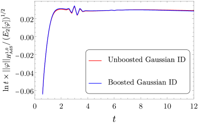
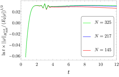
In Fig. 1 we plot the norm of the scalar field $||\varphi||_{H_{\text{AdS}}^{1,0}}$ as a function of time (see the Supplemental Material for the precise definition of the norms). According to the theorems of Holzegel and Smulevici (2013b, 2014), the late time behavior of a scalar field on a slowly rotating Kerr-AdS background should be given by

$$||\varphi||_{H^{1,0}_{\text{AdS}}}(t)=\frac{1}{\ln t}\,C\,E_{2}[\varphi]^{\frac{1}{2}}\,,$$ (12)

where $C$ is a positive constant that only depends the parameters of the background but not on the choice of initial conditions for the scalar field. Fig. 1 confirms that our initial data exhibits this inverse logarithmic decay in time. The oscillations that can been seen at around $t\sim 3$ correspond to the first time that the scalar field reaches the boundary of AdS; there is another, much smaller, oscillation at around $t\sim 6$, which corresponds to the second time that the scalar field hits the boundary. Later oscillations cannot be seen on the scale of this plot. For all different choices of initial conditions we obtain the same late time behavior; in particular, we extract the same constant $C\approx 0.03$, thus confirming that this constant only depends on the background parameters. Therefore we conclude that our choice of initial data is generic in the sense of Holzegel and Smulevici (2013b, 2014).

We now describe the backreaction of the scalar field on the geometry. We consider the initial boosted scalar field configuration described above, but with $(x_{0},y_{0},z_{0})=(0.6,0,0)$ and $(e_{x},e_{y},e_{z})=(0.1,0.3,0.6)$, and a lower amplitude of $A=0.1$ to keep the initial constraint violations sufficiently small. We observe a very rapid increase of the AH area due to the effect of the scalar perturbation; after this initial increase, the AH area remains pretty much constant for the rest of the simulation.

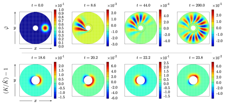
In the top panels of Fig. 2 we display four representative snapshots of the evolved scalar field $\tilde{\varphi}$ on the rotation plane $z=0$ . This sequence of plots shows how the scalar field is dragged along by the rotation of the central black hole as the evolution proceeds. We observe that, while the total amplitude of the scalar field decreases with time, at late times small distance structure develops in the region between the apparent horizon and the boundary. The reason for this is the non-linear trapping mechanism which results in a slower decay of the higher $l$ scalar harmonics. At early times the scalar field profile can be seen to be supported outside as well as in the region near and inside the black hole, penetrating the AH (see the second and third top panels in Fig. 2), and thus rapidly decaying. However, at late times the dynamics of the scalar field is very different; the last top panel in Fig. 2 shows that the high $l$ modes of the scalar field are supported in a region between the AdS boundary and a potential barrier, and the latter is at some finite distance from the horizon of the black hole. This is the reason why these large $l$ modes decay so slowly, resulting in non-linear effects.

In the bottom panels of Fig. 2 we display four representative snapshots of the spacetime Kretschmann scalar $K$ relative to that of the initial Kerr-AdS black hole, $\hat{K}$. After an initial period of adjustment, the relative Kretschmann oscillates around a central value. The size of these local deviations from Kerr-AdS is of a few percent, which is consistent with the amplitude of the initial scalar perturbation. It is interesting to note that the Kretschmann scalar rotates in the opposite direction as the scalar field; this is most easily seen in the animation showing the real time evolution of this quantity . The relative Kretschmann evolves on two periodic timescales; first, it rotates around the central black hole and then the amplitudes of local maximum and minimum themselves oscillate around a central value. The period of the global rotation of the relative Kretschmann is compatible with the light crossing time in the spacetime. Therefore, our simulations provide evidence that the relative Kretschmann exhibits what appears to be periodic dynamics, which indicates that the spacetime itself is also periodic.

Figure 3: $L^{2}$ norm of Kretschmann scalar $K$ relative to the Kretschmann scalar $\hat{K}$ of Kerr-AdS with $M=0.4$ and $a=0.2$.

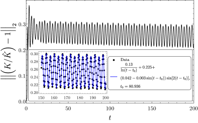
To provide further evidence, in Fig. 3 we display the evolution of the $L^{2}$ norm of the relative Kretschmann scalar. This norm is computed over the region between the AH and the boundary of AdS. Our simulations indicate that the deviation from Kerr-AdS will eventually settle down to a finite value, with oscillations of finite amplitude on top. In the inset in Fig. 3 we show that the evolution of the $L^{2}$ norm of the relative Kretschmann can be accurately captured by a fit to a function of the form

$$f(t)=\tfrac{a_{1}}{\ln(t-t_{0})}+[a_{2}+a_{3}\sin(t-t_{0})]\sin[2(t-t_{0})]+a_{4}\,,$$ (13)

where $t_{0}$ is the “late” time that we choose to do the fit, typically $t_{0}\sim 80$, but the fit is not sensitive to the choice of $t_{0}$ as long as it is large enough. The first term in (13) can be replaced by any other slowly decaying function and the fit is equally good; for instance, $e^{-a_{1}(t-t_{0})}$ or $a_{1}/(t-t_{0})$ work just as well. This first term in (13) can be interpreted as accounting for the remnant scalar field in the spacetime that is slowly decaying; the two periodic functions in (13) capture the two timescales in the evolution of the Kretschmann that can be seen in the bottom panels of Fig. 2, namely the rotation around the central black hole and the oscillation of the amplitude. More importantly, the constant term $a_{4}$ in the fit is pretty much insensitive to the choice of the slowly decaying function in the first term in (13); the possible choices outlined above all give $a_{4}\sim 0.23-0.25$. $a_{4}$ is the central value about which the $L^{2}$ norm of the relative Kretschmann is oscillating at late times, thus suggesting that the relative Kretschmann will not decay at all. This leads to the conclusion that the spacetime is not going to settle down to another member of the Kerr-AdS family of black holes.

Figure 4: Evolution of some of the $l=m$ modes of the boundary energy density $\epsilon_{\text{CFT}}$. The modes $l=m\neq 0$ are not present in Kerr-AdS and some of these modes do not decay.

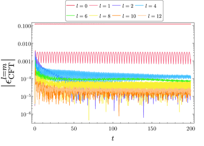
In Fig. 4 we display the amplitudes, as functions of time, of certain $l=m$ modes in the spherical harmonic decomposition of the energy density of the dual CFT. Here $\epsilon_{\text{CFT}}$ is the eigenvalue corresponding to the unique timelike eigenvector of the boundary stress-energy tensor $\langle T_{ab}\rangle_{\text{CFT}}$; we could have equally displayed $-\langle T^{t}_{\phantom{t}t}\rangle_{\text{CFT}}$ but, since the angular velocity of the black hole is small, the two quantities look qualitatively the same. The modes $l=m\neq 0$ shown in this figure are not present in Kerr-AdS and hence their amplitudes constitute a direct measurement of the deviations from Kerr-AdS. Fig. 4 shows that with our numerical resolution, the scale of the numerical noise on the mode decomposition of the boundary energy density is at around $\sim 5\times 10^{-4}$. On the scale of this plot, some modes (e.g., $l=m=1,\,4,\,6,\,8$) are well above the numerical noise levels and do not decay on the timescale of our simulation. Again, this is evidence that there is a persistent deviation from Kerr-AdS. We note that the $l=m=6$ mode exhibits some non-trivial dynamics at intermediate times, while there is a hint in our data that the $l=m=8$ mode may start to grow at late times.

Discussion.— In this article we have identified generic initial conditions for a scalar field on a fixed slowly rotating Kerr-AdS background such that, upon evolution, exhibit the required logarithmic decay in time. After turning on the backreaction of the scalar field on the spacetime metric, we find that the high $l$ modes of the scalar field are stably trapped between a certain region in the exterior of the black hole and the boundary of AdS. The modes that experience stable trapping are very long lived; in fact, the lifetime of each individual mode diverges exponentially with $l$. There appears to be a transfer of energy from the scalar field to the metric, which gives rise to a time-dependent, non-axisymmetric geometry that differs from Kerr-AdS. Furthermore, this resulting spacetime appears to be periodic and hence it does not decay to a nearby slowly rotating Kerr-AdS black hole. Therefore, our results indicate that slowly rotating Kerr-AdS black holes are non-linearly unstable.

Given the length of our simulations, we cannot ascertain whether the endpoint of the evolution is a periodic spacetime as the fit (13) would suggest, or the geometry experiences an energy cascade to the UV on a very long timescale that our simulations do not capture. Similar conclusions were reached from the numerical simulations of the superradiant instability of Kerr-AdS Chesler and Lowe (2019); Chesler (2021). A third possibility that we cannot completely rule out is that eventually the spacetime does decay to another Kerr-AdS black hole but on a much longer timescale. However, our simulations do not seem to favor this last possibility.

There are many interesting extensions of the present work. First, one would need to run longer and more accurate simulations to conclusively determine whether the geometry exhibits a runaway cascade to the UV. Ref. Dias et al. (2012) argued that smooth perturbations of slowly rotating black holes in AdS should be non-linearly stable but perturbations of low differentiability in sufficiently high dimensions could be unstable. The initial data that we used in the simulations presented in this paper is smooth; even though the spacetime does not seem to settle down to Kerr-AdS, we have not been able to identify a norm that grows at late times so it is not clear that our results contradict the conjecture of Dias et al. (2012). However, we have identified initial data that is only $C^{2}$ and preliminary results suggest that its non-linear evolution is qualitatively similar to that of the smooth initial data presented in this article. All in all, slowly rotating Kerr-AdS black holes seem to be generically non-linearly unstable.

Acknowledgements.—We would like to thank Gustav Holzegel for comments on an earlier version of this article. PF would like to thank Bob Wald for discussions. PF would also like to thank the Enrico Fermi Institute and the Department of Physics of the University of Chicago for their hospitality in the final stages of this work. PF and LR were supported by a Royal Society Fellowship URF\R\201026 and RF\ERE\210291. This work used the Young Tier 2 HPC cluster at UCL; we are grateful to the UK Materials and Molecular Modelling Hub for computational resources, which is partially funded by EPSRC (EP/P020194/1 and EP/T022213/1). Calculations were also performed using the Sulis Tier 2 HPC platform hosted by the Scientific Computing Research Technology Platform at the University of Warwick. Sulis is funded by EPSRC Grant EP/T022108/1 and the HPC Midlands+ consortium. This work also used the DiRAC@Durham facility managed by the Institute for Computational Cosmology on behalf of the STFC DiRAC HPC Facility. The equipment was funded by BEIS capital funding via STFC capital grants ST/P002293/1, ST/R002371/1 and ST/S002502/1, Durham University and STFC operations grant ST/R000832/1. DiRAC is part of the National e-Infrastructure. For the purpose of Open Access, the author has applied a CC BY public copyright licence to any Author Accepted Manuscript version arising from this submission.

Supplemental Material

AdS Norms.— In this appendix we collect the definitions of various norms that we use in the main text to measure the “size” of the scalar field in the bulk of the spacetime. Similar norms were used in the original works of Holzegel (2012); Holzegel and Smulevici (2013b, 2014).

We consider the global compactified asymptotically spherical coordinates defined in the main text $(t,\rho,\theta,\phi)$. Let $\rho_{\text{AH}}(\theta,\phi)$ denote the location of the AH on a certain $t=\text{const}$ slice $\Sigma_{t}$ so that $\Sigma_{t}^{\text{ext}}:=\Sigma_{t}\cap\left\{\rho>\rho_{\text{AH}}\right\}$ is the region outside the AH. Denote with $\sigma_{AB}$ the metric on the two-spheres at fixed $t$ and $\rho$ in coordinates $x^{A}=(\theta,\phi)$, and $D_{A}$ is the associated metric-compatible covariant derivative. Then, for any $s\in\mathbb{R}$, we define the norms

$$\left|\left|\varphi\right|\right|^{2}_{H_{\text{AdS}}^{0,s}}(t):=\int_{\Sigma_{t}^{\text{ext}}}d\mu\,R^{s}\varphi^{2}\,,$$ (S1)

$$\left|\left|\varphi\right|\right|^{2}_{H_{\text{AdS}}^{1,s}}(t):=\int_{\Sigma_{t}^{\text{ext}}}d\mu\,R^{s}\left[R^{2}(\partial_{R}\varphi)^{2}+\sigma^{AB}D_{A}\varphi D_{B}\varphi+\varphi^{2}\right]\,,$$ (S2)

$$\left|\left|\varphi\right|\right|^{2}_{H_{\text{AdS}}^{2,s}}(t):=\left|\left|\varphi\right|\right|^{2}_{H_{\text{AdS}}^{1,s}}(t)$$

$$\hskip 14.22636pt+\int_{\Sigma_{t}^{\text{ext}}}d\mu\,R^{s}\bigl{[}R^{4}(\partial_{R}\partial_{R}\varphi)^{2}+R^{2}\sigma^{AB}\left(D_{A}\partial_{R}\varphi\right)\left(D_{B}\partial_{R}\varphi\right)$$

$$\hskip 71.13188pt+\sigma^{AB}\sigma^{CD}\left(D_{A}D_{C}\varphi\right)\left(D_{B}D_{D}\varphi\right)\bigr{]}\,.$$ (S3)

where $d\mu=dRd\theta d\phi R^{2}\sin\theta$ is the integration volume and we have used the uncompactified radial coordinate $R=2\rho/(1-\rho^{2})$ to allow for a straightforward comparison with the definitions in Holzegel (2012).

In our simulations we also compute the following “energy” norms at $t=0$, defined similarly to Holzegel and Smulevici (2013b, 2014) after replacing their coordinates with our $(t,R,\theta,\phi)$,

$$E_{1}[\varphi]:= \left|\left|\varphi\right|\right|^{2}_{H_{\text{AdS}}^{1,0}}(0)+\left|\left|\partial_{t}\varphi\right|\right|^{2}_{H_{\text{AdS}}^{0,-2}}(0)$$ (S4)

$$E_{2}[\varphi]:= \left|\left|\varphi\right|\right|^{2}_{H_{\text{AdS}}^{2,0}}(0)+\left|\left|\partial_{t}\varphi\right|\right|^{2}_{H_{\text{AdS}}^{1,0}}(0)$$

$$+\sum_{i=1}^{3}\left|\left|m_{i}(\varphi)\right|\right|^{2}_{H_{\text{AdS}}^{1,0}}(0)+\left|\left|\partial_{t}\partial_{t}\varphi\right|\right|^{2}_{H_{\text{AdS}}^{0,-2}}(0),$$ (S5)

where $m_{1}=\frac{\partial}{\partial\phi}$, $m_{2}=-\sin\phi\frac{\partial}{\partial\theta}-\cot\theta\cos\phi\frac{\partial}{\partial\phi}$, $m_{3}=\cos\phi\frac{\partial}{\partial\theta}-\cot\theta\sin\phi\frac{\partial}{\partial\phi}$ are the standard generators of $SO(3)$ rotations.

Numerical tests.— In this appendix we present some numerical tests to assess the accuracy and convergence of our code. The code that we have used is essentially the same as in Bantilan et al. (2021), and more thorough convergence tests can be found in this reference.

Figure S1: Inverse logarithmic decay of $||\varphi||_{H^{1,0}_{\text{AdS}}}$ for unboosted initial data for three different resolutions.

First we consider the convergence tests; we focus on the case without backreaction because of the prohibitive cost of the simulations in the fully non-linear case. We consider Gaussian initial data (without boost) for the scalar field, with the same parameters as in the main text, on a Kerr-AdS background with $M=0.4$ and $a=0.2$. We evolve this initial data for different resolutions and Fig. S1 shows the logarithmic decay in each case.

Figure S2: Convergence factor obtained from the data in Fig. S1.

Using this simulations, we compute the convergence factor,

$$Q\left[f\right]:=\frac{1}{\ln(3/2)}\ln\left(\left|\frac{f_{N=145}-f_{N=217}}{f_{N=217}-f_{N=325}}\right|\right)$$ (S6)

as a function of time, where $f=\ln t\times||\varphi||_{H^{1,0}_{\text{AdS}}}/(E_{2}[\varphi])^{\frac{1}{2}}$ and $f_{N}$ denotes the numerical values of $f$ in the simulation with $N$ points along each direction of the Cartesian grid. The result is shown in Fig. S2. Given the discretization scheme used in our code, one should expect second order convergence, and hence $Q\left[f\right]=2$. Fig. S2 confirms that, after an initial rapid period of adjustment, our code converges at the expected order throughtout the rest of the simulation.

Figure S3: Evolution of the conserved charges and the $L^{2}$ norm of the trace of the energy-momentum tensor of the dual CFT.

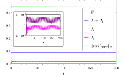
An important check of the accuracy of our numerical simulations with backreaction is to verify that the conserved charges are truly conserved in practice (and hence that we are solving the equations of motion accurately). In Fig. S3 we display the evolution of the total energy $E$ and angular momentum $J$ as functions of time. This figure shows that these quantities do stay constant throughout the evolution after a brief initial period of gauge adjustment, during which the constraint violations are exponentially damped. We also display the evolution of the other components of the angular momentum, which should be zero in the continuum limit; in our simulations they are $O(10^{-4})$ at all times. Finally, we also show the evolution of the $L^{2}$ norm of the trace of the boundary energy-momentum tensor, $||\langle\text{tr}T\rangle_{CFT}||_{2}$, which should also be zero in the continuum limit; this quantity is of a few percent level at all times. We point out that the local values of $|\langle\text{tr}T\rangle_{CFT}|$ are $O(10^{-4})$, so much smaller than the $L^{2}$ norm of this quantity. These tests confirm the correctness of our simulations.

References

- Maldacena (1999) J. M. Maldacena, Int. J. Theor. Phys. 38, 1113 (1999), [Adv. Theor. Math. Phys.2,231(1998)], arXiv:hep-th/9711200 [hep-th] .
- Gubser et al. (1998) S. S. Gubser, I. R. Klebanov, and A. M. Polyakov, Phys. Lett. B428, 105 (1998), arXiv:hep-th/9802109 [hep-th] .
- Witten (1998) E. Witten, Adv. Theor. Math. Phys. 2, 253 (1998), arXiv:hep-th/9802150 [hep-th] .
- Christodoulou and Klainerman (1993) D. Christodoulou and S. Klainerman, “The Global Nonlinear Stability of Minkwoski Space,” (Princeton University Press, 1993).
- Dafermos (2006) M. Dafermos, “The black hole stability problem,” ((2006)).
- Dafermos and Holzegel (2006) M. Dafermos and G. Holzegel, “Dynamic instability of solitons in 4+1-dimensional gravity with negative cosmological constant,” (unpublished - available at https://www.dpmms.cam.ac.uk/~md384/ADSinstability.pdf (2006)).
- Note (1) On the other hand, AdS is expected to be stable with dissipative boundary conditions Holzegel et al. (2019).
- Bizoń and Rostworowski (2011) P. Bizoń and A. Rostworowski, Phys. Rev. Lett. 107, 031102 (2011), arXiv:1104.3702 [gr-qc] .
- Moschidis (2020) G. Moschidis, Anal. Part. Diff. Eq. 13, 1671 (2020), arXiv:1704.08681 [gr-qc] .
- Moschidis (2018) G. Moschidis, (2018), arXiv:1812.04268 [math.AP] .
- Policastro et al. (2001) G. Policastro, D. T. Son, and A. O. Starinets, Phys. Rev. Lett. 87, 081601 (2001), arXiv:hep-th/0104066 .
- Kovtun et al. (2003) P. Kovtun, D. T. Son, and A. O. Starinets, JHEP 10, 064 (2003), arXiv:hep-th/0309213 .
- Kovtun et al. (2005) P. Kovtun, D. T. Son, and A. O. Starinets, Phys. Rev. Lett. 94, 111601 (2005), arXiv:hep-th/0405231 .
- Baier et al. (2008) R. Baier, P. Romatschke, D. T. Son, A. O. Starinets, and M. A. Stephanov, JHEP 04, 100 (2008), arXiv:0712.2451 [hep-th] .
- Bhattacharyya et al. (2008) S. Bhattacharyya, V. E. Hubeny, S. Minwalla, and M. Rangamani, JHEP 02, 045 (2008), arXiv:0712.2456 [hep-th] .
- Berti et al. (2009) E. Berti, V. Cardoso, and A. O. Starinets, Class. Quant. Grav. 26, 163001 (2009), arXiv:0905.2975 [gr-qc] .
- Cardoso et al. (2014) V. Cardoso, O. J. C. Dias, G. S. Hartnett, L. Lehner, and J. E. Santos, JHEP 04, 183 (2014), arXiv:1312.5323 [hep-th] .
- Bantilan et al. (2012) H. Bantilan, F. Pretorius, and S. S. Gubser, Phys. Rev. D85, 084038 (2012), arXiv:1201.2132 [hep-th] .
- Chesler and Yaffe (2014) P. M. Chesler and L. G. Yaffe, JHEP 07, 086 (2014), arXiv:1309.1439 [hep-th] .
- Chesler and Lowe (2019) P. M. Chesler and D. A. Lowe, Phys. Rev. Lett. 122, 181101 (2019), arXiv:1801.09711 [gr-qc] .
- Bantilan et al. (2021) H. Bantilan, P. Figueras, and L. Rossi, Phys. Rev. D 103, 086006 (2021), arXiv:2011.12970 [hep-th] .
- Chesler (2021) P. M. Chesler, (2021), arXiv:2109.06901 [gr-qc] .
- Holzegel (2010) G. Holzegel, Commun. Math. Phys. 294, 169 (2010), arXiv:0902.0973 [gr-qc] .
- Holzegel and Smulevici (2012) G. Holzegel and J. Smulevici, Annales Henri Poincare 13, 991 (2012), arXiv:1103.0712 [gr-qc] .
- Holzegel (2012) G. Holzegel, J. Hyperbol. Diff. Equat. 9, 239 (2012), arXiv:1103.0710 [gr-qc] .
- Holzegel and Smulevici (2013a) G. Holzegel and J. Smulevici, Commun. Math. Phys. 317, 205 (2013a), arXiv:1103.3672 [gr-qc] .
- Holzegel and Smulevici (2013b) G. Holzegel and J. Smulevici, Commun. Pure Appl. Math. 66, 1751 (2013b), arXiv:1110.6794 [gr-qc] .
- Holzegel and Warnick (2014) G. H. Holzegel and C. M. Warnick, J. Funct. Anal. 266, 2436 (2014), arXiv:1209.3308 [gr-qc] .
- Holzegel and Smulevici (2014) G. Holzegel and J. Smulevici, Anal. Part. Diff. Eq. 7, 1057 (2014), arXiv:1303.5944 [gr-qc] .
- Note (2) Other types of allowed boundary conditions, such as introducing sources for the fields at the conformal boundary, lead to new gravitational dynamics in the bulk, which do not have asymptotically flat space analogues, but they should be less surprising.
- Carter (1968) B. Carter, Commun. Math. Phys. 10, 280 (1968).
- Kerr (1963) R. P. Kerr, Phys. Rev. Lett. 11, 237 (1963).
- Press and Teukolsky (1973) W. H. Press and S. A. Teukolsky, Astrophys. J. 185, 649 (1973).
- Chandrasekhar (1984) S. Chandrasekhar, Fundam. Theor. Phys. 9, 5 (1984).
- Whiting (1989) B. F. Whiting, J. Math. Phys. 30, 1301 (1989).
- Dafermos and Rodnianski (2010) M. Dafermos and I. Rodnianski, (2010), arXiv:1010.5132 [gr-qc] .
- Dafermos et al. (2016) M. Dafermos, I. Rodnianski, and Y. Shlapentokh-Rothman, Annals of Math. 183, 787 (2016), arXiv:1402.7034 [gr-qc] .
- Klainerman and Szeftel (2022a) S. Klainerman and J. Szeftel, Ann. PDE 8, 17 (2022a), arXiv:1911.00697 [math.AP] .
- Klainerman and Szeftel (2022b) S. Klainerman and J. Szeftel, Ann. PDE 8, 18 (2022b), arXiv:1912.12195 [math.AP] .
- Giorgi et al. (2020) E. Giorgi, S. Klainerman, and J. Szeftel, (2020), arXiv:2002.02740 [math.AP] .
- Dafermos et al. (2021) M. Dafermos, G. Holzegel, I. Rodnianski, and M. Taylor, (2021), arXiv:2104.08222 [gr-qc] .
- Klainerman and Szeftel (2023) S. Klainerman and J. Szeftel, Pure Appl. Math. Quart. 19, 791 (2023), arXiv:2104.11857 [math.AP] .
- Dafermos et al. (2022) M. Dafermos, G. Holzegel, I. Rodnianski, and M. Taylor, (2022), arXiv:2212.14093 [gr-qc] .
- Giorgi et al. (2022) E. Giorgi, S. Klainerman, and J. Szeftel, “Wave equations estimates and the nonlinear stability of slowly rotating kerr black holes,” (2022), arXiv:2205.14808 [math.AP] .
- Niehoff et al. (2016) B. E. Niehoff, J. E. Santos, and B. Way, Class. Quant. Grav. 33, 185012 (2016), arXiv:1510.00709 [hep-th] .
- Kim et al. (2023) S. Kim, S. Kundu, E. Lee, J. Lee, S. Minwalla, and C. Patel, (2023), arXiv:2305.08922 [hep-th] .
- Hawking and Reall (2000) S. W. Hawking and H. S. Reall, Phys. Rev. D 61, 024014 (2000), arXiv:hep-th/9908109 .
- Wald (1984) R. M. Wald, General Relativity (Chicago Univ. Pr., Chicago, USA, 1984).
- Pretorius (2005) F. Pretorius, Class. Quant. Grav. 22, 425 (2005), arXiv:gr-qc/0407110 [gr-qc] .
- Figueras and Rossi (2023) P. Figueras and L. Rossi, to appear (2023).
- Bantilan et al. (2017) H. Bantilan, P. Figueras, M. Kunesch, and P. Romatschke, Phys. Rev. Lett. 119, 191103 (2017), arXiv:1706.04199 [hep-th] .
- Bantilan et al. (2020) H. Bantilan, P. Figueras, and D. Mateos, Phys. Rev. Lett. 124, 191601 (2020), arXiv:2001.05476 [hep-th] .
- Rossi (2022) L. Rossi, Numerical Cauchy evolution of asymptotically AdS spacetimes with no symmetries, Ph.D. thesis, Queen Mary, U. of London (2022), arXiv:2205.15329 [gr-qc] .
- Gibbons et al. (2005) G. W. Gibbons, H. Lu, D. N. Page, and C. N. Pope, J. Geom. Phys. 53, 49 (2005), arXiv:hep-th/0404008 .
- Note (3) Http://laplace.physics.ubc.ca/Group/Software.html.
- Note (4) For an animation, see https://www.youtube.com/watch?v=dH0InwWvtso.
- Note (5) https://www.youtube.com/watch?v=fbj6DUglEqc.
- Dias et al. (2012) O. J. C. Dias, G. T. Horowitz, D. Marolf, and J. E. Santos, Class. Quant. Grav. 29, 235019 (2012), arXiv:1208.5772 [gr-qc] .
- Note (6) Www.dirac.ac.uk.
- Holzegel et al. (2019) G. Holzegel, J. Luk, J. Smulevici, and C. Warnick, Commun. Math. Phys. 374, 1125 (2019), arXiv:1502.04965 [gr-qc] .