GigaPose: Fast and Robust Novel Object Pose Estimation via One Correspondence

Abstract

We present GigaPose, a fast, robust, and accurate method for CAD-based novel object pose estimation in RGB images. GigaPose first leverages discriminative “templates”, rendered images of the CAD models, to recover the out-of-plane rotation and then uses patch correspondences to estimate the four remaining parameters. Our approach samples templates in only a two-degrees-of-freedom space instead of the usual three and matches the input image to the templates using fast nearest-neighbor search in feature space, results in a speedup factor of 38$\times$ compared to the state of the art. Moreover, GigaPose is significantly more robust to segmentation errors. Our extensive evaluation on the seven core datasets of the BOP challenge demonstrates that it achieves state-of-the-art accuracy and can be seamlessly integrated with a refinement method. Additionally, we show the potential of GigaPose with 3D models predicted by recent work on 3D reconstruction from a single image, relaxing the need for CAD models and making 6D pose object estimation much more convenient. Our source code and trained models are publicly available at https://github.com/nv-nguyen/gigaPose.

1 Introduction

6D object pose estimation has significantly improved over the past decade [20, 46, 49, 26, 55, 22, 51, 30]. However, supervised deep learning methods, despite remarkable accuracy, are cumbersome to deploy to an industrial setting. Indeed, for each novel object, the pose estimation model needs to be retrained using newly-acquired data, which is impractical: Retraining typically takes several hours or days [22, 30], and the end users might not have the skills to retrain the model.

To fulfill the needs of such industrial settings, CAD-based novel object pose estimation, which focuses on estimating the 6D pose of novel objects (i.e., objects only available at inference time, not during training), has garnered attention and was introduced in the latest BOP challenge [2]. Current approaches involve three main steps: object detection and segmentation, coarse pose estimation, and refinement. While object detection and segmentation has been recently addressed by CNOS [36], refinement has been also addressed effectively with render-and-compare approaches [23, 50]. However, existing solutions to coarse pose estimation still suffer from low inference speed and sensitivity to segmentation errors. We thus focus on this step in this paper.

The low inference speed stems from how existing coarse pose estimation methods rely on templates [37, 56, 23]. Among them, MegaPose [23] has been widely adopted and integrated into various pipelines, notably the BOP challenge-winner GenFlow [2] . However, the complexity of MegaPose is linear in the number of templates, as it matches the input images against the templates by running a network on each image-template pair. As a result, the methods based on MegaPose require more than 1.6 seconds per detection.

Sensitivity to detection and segmentation errors, often due to occlusions, is a common issue for template-based approaches [37, 23]. As illustrated in Figure 1, the segmentation of occluded objects such as the “duck” (left example), results in a scale and translation mismatch when cropping the test image and templates. Additionally, the erroneous segments may include noisy signal from the other objects or the background, which results in numerous outlier matches between the input image and the templates.

To address these two major limitations, we introduce GigaPose, a novel approach for CAD-based coarse object pose estimation. GigaPose makes several technical contributions towards speed and robustness and can be seamlessly integrated with any refinement method for CAD-based novel object pose estimation to achieve state-of-the-art accuracy.

The key idea in GigaPose is to find the right trade-off between the use of templates, which have been shown to be extremely useful for estimating the pose of novel objects, and patch correspondences, which lead to better robustness and more accurate pose estimates. More precisely, we propose to rely on templates to estimate two degrees of freedom (DoFs)—azimuth and elevation—as varying these angles changes the appearance of an object in complex ways, which templates excel at capturing effectively. Our templates are represented with local features that are trained to be robust to scaling and in-plane rotations. Matching the input image with the templates based on these local features yields robustness to segmentation errors.

To estimate the remaining 4 DoFs—in-plane rotation and 3D translation decomposed into 2D translation and 2D scale, we rely on patch correspondences between the input image and the template candidates. Given a template candidate, we match its local features with those of the input image, which gives us 2D-2D point correspondences. Instead of simply exploiting the matched point coordinates and use a P$n$P algorithm [35] to estimate the pose as done in previous works [46, 17, 18], we also exploit their appearances: We show that it is possible to predict the in-plane rotation and relative scale between the input image and the template from local features computed at the matched points. The remaining 2D translation is obtained from the positions of these matched points, allowing the estimation of the four DoFs from a single correspondence. To robustify this estimate, we combine this process with RANSAC.

We experimentally demonstrate that our balance between the use of templates and patch correspondences effectively addresses the two issues in coarse pose estimation. Indeed, our method relies on a sublinear nearest-neighbor template search, successfully addressing the low inference speed issue with a speedup factor of 38$\times$ per detection compared to to MegaPose [23]. Furthermore, the two steps of our method are particularly robust to segmentation errors.

We also demonstrate that GigaPose can exploit a 3D model reconstructed from a single image by a diffusion-based model [32, 31, 29, 45, 44, 52] instead of an accurate CAD model. Despite the inaccuracies of the predicted 3D models, our method can recover an accurate 6D pose as shown on Figure 1. This relaxes the need for CAD models and makes 6D pose object detection much more convenient.

In summary, our contribution is a novel RGB-based method for CAD-based novel object coarse pose estimation from a single correspondence that is significantly faster, more robust, and more accurate than existing methods. We demonstrate this through extensive experiments on the seven core datasets of the BOP challenge [48].

2 Related Work

Seen object pose estimation. Early works on 6D pose estimation have introduced diverse benchmarks to evaluate the performance of their approaches [3, 14, 15, 8, 10, 19, 54, 48]. This data and its ground truth have powered many deep learning-based methods [20, 46, 26, 49, 27, 55, 41, 17, 22, 30]. Some of them show remarkable performance in terms of run-time and accuracy [22, 30]. However, these approaches require long and expensive training, such as the state-of-the-art methods [22, 30] require several hours for training for a single object, making them too cumbersome for many practical applications in robotics and AR/VR.

To avoid the need for re-training when dealing with new object instances, one approach is to train on object categories by assuming that the testing objects belong to a known category [28, 53, 6, 25, 33, 34]. These category-level pose estimation methods, however, cannot generalize to objects beyond the scope of the training categories. By contrast, our method operates independently of any category-level information and seamlessly generalizes to novel categories.

Figure 2: Overview. We first onboard each novel object by rendering 162 templates, spanning the spectrum of out-of-plane rotations. We also extract dense features using ${\bf F}_{\text{ae}}$ from each of the templates. At runtime, given a query image segmented with CNOS [36], we process it (by masking the background, cropping on the segment, adding padding then resizing), and extracting features with ${\bf F}_{\text{ae}}$. We retrieve the nearest template to the segment using the similarity metric detailed in Section 3.2. Further, 2D scale and in-plane rotation are computed from a single 2D-2D correspondence using ${\bf F}_{\text{ist}}$ and two lightweight MLPs. The 2D position of the correspondences also gives us the 2D translation which is used with 2D scale, in-plane rotation to create the affine transformation ${\bf M}_{t\rightarrow q}$, mapping the nearest template to the query image. This enables us to recover the complete 6D object pose from a single correspondence. Finally, we use RANSAC to robustly find the best pose candidate. Onboarding takes 17.1 seconds per object and inference takes 48 milliseconds per detection on average.

Novel object pose estimation. Several techniques have been explored to improve the generalization of CAD-based object pose estimation [43, 1, 38, 37, 56, 47, 50, 23]. These can be roughly divided into feature-matching methods [43, 1] and template matching ones [38, 37, 56, 47, 23, 1]. Feature-matching methods extract local features from the image, match them to the given 3D model and then use a variant of the P$n$P algorithm [35] to recover the 6D pose from the estimated 3D-to-2D correspondences. By contrast, template matching methods first render synthetic templates of the CAD models, and then use a deep network to compute a score for each input image-template pair, thus aiming to find the template with the most similar pose to the input image.

At the last BOP challenge [2], CAD-based novel object pose estimation was introduced as a new task, using CNOS [36] as the default detection method. MegaPose [23] and ZS6D [1] showed promising results for this new task. Nevertheless, MegaPose’s run-time was highlighted as a significant limitation due to the need for a forward pass through a coarse pose estimator to compute a classification score for every (query, template) comparison. ZS6D relies on DINOv2 features [40] and the similarity metric of [37] to predict sparse 3D-to-2D correspondences. Unfortunately, their experiments do not evaluate the model’s sensitivity to segmentation errors. In contrast, we present extensive evaluations and demonstrate that GigaPose outperforms both MegaPose and ZS6D. Our method can also be seamlessly integrated with any refinement method.

Correspondence-based object pose estimation. A classical approach to solving the 6D object pose estimation problem is to establish 3D-to-2D correspondences and compute the pose with a P$n$P algorithm [46, 49, 18, 17, 55, 42, 27], which requires at least four 3D-to-2D point correspondences. Because we first match the input image against templates and estimate the four remaining DoFs from a single 2D-to-2D match, we only need one correspondence to determine the 6D object pose. Our experimental evaluation shows that our method outperforms ZS6D, which, as stated above, is a state-of-the-art method relying on 3D-to-2D correspondences.

3 Method

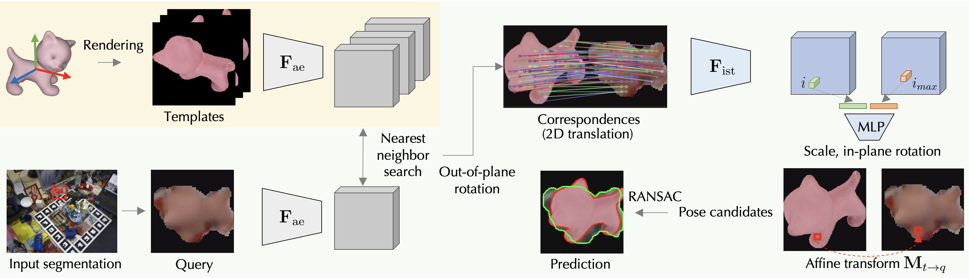
Figure 3 provides an overview of GigaPose. Given the 3D model of an object of interest, we render templates and extract their dense features using a Vision-Transformer (ViT) model ${\bf F}_{\text{ae}}$. Then, given an input image, we detect the object of interest and segment it using an off-the-shelf method CNOS [36]. GigaPose extracts dense features from the input image at the object location using ${\bf F}_{\text{ae}}$ again. We select the template most similar to the input image using a similarity metric based on the dense features, detailed in Section 3.2. This gives us the azimuth and elevation of the camera.

To estimate the remaining DoFs, we look for corresponding patches between the input image and its most similar template. From one such pair of patches, we can directly predict two additional DoFs: the 2D scale $s$ and the in-plane rotation $\alpha$, by feeding two lightweight MLPs the features for the two patches extracted by another feature extractor denoted as ${\bf F}_{\text{ist}}$. Note that the features extracted by ${\bf F}_{\text{ae}}$ are not suitable here, as they discard information about scale and in-plane rotation by design. The image locations of the corresponding patches also give us directly the last two DoFs: the 2D translation $({\bf t}_{x},{\bf t}_{y})$. From the scale and 2D translation, we can estimate the 3D translation. We use a RANSAC framework and iterate over different pairs of patches to find the optimal pose. We detail the training of ${\bf F}_{\text{ist}}$ and the MLPs, and the RANSAC scheme in Section 3.3.

Figure 3: Contrastive training of ${\bf F}_{\text{ae}}$. We use pairs made of a query image and a template to train a network using local contrastive learning as detailed in Section 3.2. Middle: Training samples provided by [23], and the 2D-2D correspondences created from ground-truth 3D information used to generate positive and negative pairs. Right: We seek local features that vary with the out-of-plane rotation, but are invariant to in-plane rotation and scaling. Thus, positive pairs are made of corresponding patches under scaling and in-plane rotation changes, and negative pairs are made of corresponding patches under different out-of-plane rotations, patches that do not correspond, or that come from different objects.

3.1 Generating Templates

In contrast to other approaches [37, 56], we do not generate templates for both in-plane and out-of-plane rotations, as this yields thousands of templates. Instead, we decouple the 6 DoFs object pose into out-of-plane rotation, in-plane rotation, and 3D translation (2D translation and scale). Given the out-of-plane rotation, finding the scale and in-place rotation is indeed a 2D problem only. We thus create much less templates and push the estimation of the other DoFs to a later stage in the pipeline (see Section 3.3).

In practice, we use 162 templates. These are generated from viewpoints defined in a regular icosphere which is created by subdividing each triangle of the icosphere primitive of Blender into four smaller triangles. This has been shown in previous works [36, 1, 37] to provide well-distributed view coverage of CAD models.

3.2 Predicting Azimuth and Elevation

Training the feature extractor ${\bf F}_{\text{ae}}$.

${\bf F}_{\text{ae}}$ extracts dense features from both the input image and each of the templates independently. Compared to estimating features jointly, this approach eliminates the need for extensive feature extraction at runtime, a process that scales linearly with the number of templates and in-plane rotations considered. Instead, we can offload the computation of the features for each template to an onboarding stage for each novel object. We now describe how we train the feature extractor ${\bf F}_{\text{ae}}$ and how we design the similarity metric to compare the template and query features.

The extracted features aim to match a query image to a set of templates with different out-of-plane rotations, but with fixed scale, in-plane rotation, and translation. The features should thus be invariant to scale, in-plane rotation, and 2D translation, but be sensitive to out-of-plane rotation.

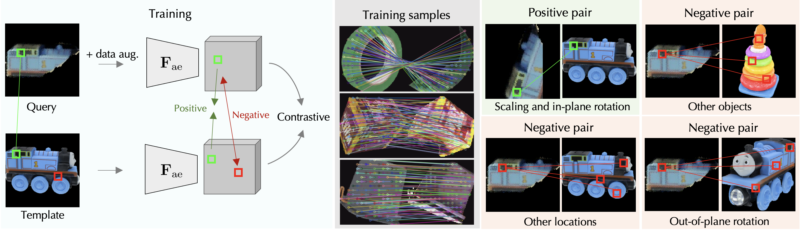
We achieve this with a local contrastive learning scheme. The main difficulty lies in defining the positive and negative patch pairs. Figure 3 illustrates our training procedure. We construct batches of $B$ image pairs $(\mathcal{Q}_{k},\mathcal{T}_{k})$, such that the query $\mathcal{Q}_{k}$ is a rendering of a 3D object in any pose, and the template $\mathcal{T}_{k}$ is another rendering of that object with the same out-of-plane rotation but different in-plane rotation, scale, and 2D translation. Because we have access to the 3D model, we can compute ground-truth 2D-to-2D correspondences to create positive and negative pairs. We detail in the supplementary material how we compute these correspondences.

Additionally, since our goal is to close the domain gap between real images and synthetic renderings, we apply color augmentation along with random cropping and in-plane rotation to the input pairs. We use the training sets provided by the BOP challenge [48], originally sourced from MegaPose [23]. These datasets consist of 2 million images and are generated from CAD models of Google Scanned Objects [9] and ShapeNet [5] using BlenderProc [7]. We show typical training samples in the middle part of Figure 3.

We pass each image $\mathcal{Q}_{k}$ and $\mathcal{T}_{k}$ independently through ${\bf F}_{\text{ae}}$ to extract dense feature maps ${\bf q}_{k}$ and ${\bf t}_{k}$. Below, we use the superscript $i$ to denote a 2D location in the local feature map. Note that because of the downsizing done by the ViT, each location $i$ in the feature grid corresponds to a 14$\times$14 patch in the respective input image. Each feature map has a respective segmentation mask ${\bf m}_{{\cal Q}_{k}}$ and ${\bf m}_{{\cal T}_{k}}$ corresponding to the foreground of the object in the images $\mathcal{Q}_{k}$ and $\mathcal{T}_{k}$.

For a location $i$ in the query feature map ${\bf q}_{k}$, we denote by $i^{*}$ the corresponding location in the template feature map. We arrange the query patches $({\bf q}_{k}^{i})$ and their corresponding patch $({\bf t}_{k}^{i^{*}})$ in a square matrix such that the diagonal contains the positive pairs, and all other entries serve as negative pairs. For each pair $(\mathcal{Q}_{k},\mathcal{T}_{k})$, we thus obtain $|{\bf m}_{{\cal Q}_{k}}|$ positive pairs and $|{\bf m}_{{\cal Q}_{k}}|\times(|{\bf m}_{{\cal Q}_{k}}|-1)$ negative pairs.

To improve the efficiency of contrastive learning, we use additional negative pairs from a query image $\mathcal{Q}_{k}$ and a template $\mathcal{T}_{k^{\prime}}$, where $k^{\prime}\neq k$ in the current batch. This process results in total in $\left(\sum_{k=1}^{B}|{\bf m}_{{\cal Q}_{k}}|\right)^{2}-\sum_{k=1}^{B}|{\bf m}_{{\cal Q}_{k}}|$ negative pairs for the current batch. We train ${\bf F}_{\text{ae}}$ to align the representations of the positive pairs while separating the negative pairs using the InfoNCE loss [39]:

$${\cal L}_{\text{out}}=-\sum_{k=1}^{B}\sum_{i=1}^{|{\bf m}_{{\cal Q}_{k}}|}\ln\frac{e^{S({\bf q}_{k}^{i},{\bf t}_{k}^{i^{*}})/\tau}}{\sum_{(k^{\prime},i^{\prime})\neq(k,i^{*})}e^{S({\bf q}_{k}^{i},{\bf t}_{k^{\prime}}^{i^{\prime}})/\tau}}\>,$$ (1)

where $S(.,.)$ is the cosine similarity between the local image features computed by the network ${\bf F}_{\text{ae}}$. The temperature parameter $\tau$ is set to $0.1$ in our experiments.

Since the positive pairs of patches have different scales and in-plane rotations, our network ${\bf F}_{\text{ae}}$ learns to become invariant to these two factors, as demonstrated in our experiments. We initialize our feature extractor ${\bf F}_{\text{ae}}$ as DINOv2 [40] pretrained on ImageNet, because it has proven to be highly effective in extracting features for vision tasks.

Azimuth and elevation prediction.

We define a pairwise similarity metric for each query-template $(\mathcal{Q},\mathcal{T})$ pair with their respective dense feature grid $({\bf q},{\bf t})$ and feature segmentation masks $(\text{m}_{\cal Q},\text{m}_{\cal T})$.

For each local query feature ${\bf q}^{i}$, corresponding to patch at location $i$, we compute its nearest neighbor in the template features ${\bf t}$, denoted as ${\bf t}^{i_{\text{max}}}$, as

$$i_{\text{max}}=\operatorname*{arg\,max}_{{j|\text{m}_{\mathcal{T}}^{j}>0}}S\left({\bf q}^{i},{\bf t}^{j}\right)\>.$$ (2)

This nearest neighbor search yields a list of correspondences $\{({i,i_{\text{max}}})\}$. To improve the robustness of our method against outliers, we keep only the correspondences $\{({i,i_{\text{max}}})\}$ having a similarity score $\geq$ 0.5. The final similarity for this ($\mathcal{Q}$, $\mathcal{T}$) pair is defined as the mean of all the remaining correspondences, weighted by their similarity score:

$$\operatorname{sim}({\bf q},{\bf t})=\frac{1}{|\text{m}_{\mathcal{Q}}|}\sum_{i}\text{m}_{\mathcal{Q}}^{i}S\left({\bf q}^{i},{\bf t}^{i_{\text{max}}}\right)\>.$$ (3)

We compute this score for all templates $\mathcal{T}_{k}$ ($1\leq k\leq 162$) and find the top-$K$ candidates yielding the most similar out-of-plane rotations. This nearest neighbor search is very fast and delivers results within 48 milliseconds. In practice, we experiment with $K=1$ and $K=5$. For the latter, the final template is selected by the RANSAC-based estimation detailed in Section 3.3 below.

3.3 Predicting the Remaining DoFs

Once we have identified the template candidates, we seek to estimate the remaining 4 DoFs, i.e., in-plane rotation, scale, and 2D translation, which yield the affine transformation ${\bf M}_{t\rightarrow q}$ transforming each template candidate $\mathcal{T}$ to the query image $\mathcal{Q}$. Specifically, we have

$${\bf M}_{t\rightarrow q} =\begin{bmatrix}s\cos(\alpha)&-s\sin(\alpha)&{\bf t}_{x}\\ s\sin(\alpha)&s\cos(\alpha)&{\bf t}_{y}\\ 0&0&1\\ \end{bmatrix}\>,$$ (4)

where $s$ is the 2D scaling factor, $\alpha$ is the relative in-plane rotation, and $\left[\mathbf{t}_{x},\mathbf{t}_{y}\right]$ is the 2D translation between the input query image $\mathcal{Q}$ and the template $\mathcal{T}$.

Training the feature extractor ${\bf F}_{\text{ist}}$ and the MLP.

We have already obtained from the features of ${\bf F}_{\text{ae}}$ a list of 2D-2D correspondences $\{({i,i_{\text{max}}})\}$. Each correspondence can inherently provide 2D translation $\left[\mathbf{t}_{x},\mathbf{t}_{y}\right]$ information through the patch locations $i$ and $i_{\text{max}}$. To recover the remaining 2 DoFs, scale $\mathbf{s}$ and in-plane rotation $\alpha$, we train deep networks to directly regress these values from a single 2D-2D correspondence. Since the feature extractor ${\bf F}_{\text{ae}}$ is invariant to in-plane rotation and scaling, the corresponding features cannot be used to regress those values, hence we have to train another feature extractor we call ${\bf F}_{\text{ist}}$. Given a 2D-2D match from a pair $(\mathcal{Q},\mathcal{T})$, and their corresponding feature computed by ${\bf F}_{\text{ist}}$, we pass them through two small MLPs, which outputs directly $\alpha$ and $\mathbf{s}$. This enables us to predict 2D scale and in-plane rotations for each 2D-2D correspondence. To address the $2\pi$ periodicity of in-plane rotation, we predict $\left[\cos(\alpha_{k}^{l}),\sin(\alpha_{k}^{l})\right]$ instead of $\alpha_{k}^{l}$.

We train jointly both ${\bf F}_{\text{ist}}$ and the MLPs on the same data samples as ${\bf F}_{\text{ae}}$ using the loss:

$${\cal L}_{\text{inp}}=\sum_{k=1}^{B}\sum_{i=1}^{n_{k}}\left[\left(\ln(s_{k}^{i})-\ln(s_{k}^{*})\right)^{2}+\text{geo}(\alpha_{k}^{i},\alpha_{k}^{*})\right],$$ (5)

where $s_{k}^{*}$ and $\alpha_{k}^{*}$ are the ground-truth scale and in-plane rotation between $\mathcal{Q}$ and $\mathcal{T}_{k}$, and $\text{geo}(\cdot,\cdot)$ indicates the geodesic loss defined as

$$\text{geo}(\alpha_{1},\alpha_{2})=\text{acos}\bigl{(}\text{cos}(\alpha_{1})\text{cos}(\alpha_{2})+\text{sin}(\alpha_{1})\text{sin}(\alpha_{2})\bigr{)}\>.$$ (6)

RANSAC-based ${\bf M}_{t\rightarrow q}$ estimation.

For each template $\mathcal{T}$, we employ RANSAC on each ${\bf M}_{t\rightarrow q}$ predicted by each correspondence and validate them against the remaining correspondences using a 2D error threshold of $\delta$. In practice, we set $\delta$ to the size of a patch, corresponding to an error of 14 pixels in image space. The final prediction for ${\bf M}_{t\rightarrow q}$ is determined by the correspondence with the highest number of inliers. The complete 6D object pose can finally be recovered from the out-of-plane rotation, in-plane rotation, 2D scale and 2D translation using the explicit formula provided in the supplementary material.

We initialize ${\bf F}_{\text{ist}}$ with a modified version of ResNet18 [12] instead of the DINOv2 [40] as DINOv2 is trained with random augmentations that includes in-plane rotations and cropping, making its features invariant to scale and in-plane rotation. Similarly to the features from ${\bf F}_{\text{ae}}$, we offload the feature computation of ${\bf F}_{\text{ist}}$ to the onboarding stage for all templates to avoid the computational burden at runtime.

Method Detections Refinement lm-o t-less tud-l ic-bin itodd hb ycb-v Mean Run-time                             Num. instances: 1445 6423 600 1786 3041 1630 4123 1 OSOP [47] OSOP [47] – 27.4 40.3 – – – – 29.6 – – 2 MegaPose [23] Mask R-CNN [11] – 18.7 19.7 20.5 15.3 8.00 18.6 13.9 16.2 – 3 ZS6D [1] CNOS[36] – 29.8 21.0 – – – – 32.4 – – 4 MegaPose [23] CNOS [36] – 22.9 17.7 25.8 15.2 10.8 25.1 28.1 20.8 15.5 s 5 GigaPose (Ours) CNOS [36] – 29.9 27.3 30.2 23.1 18.8 34.8 29.0 27.6 0.9 s 6 MegaPose [23] CNOS [36] MegaPose [23] 49.9 47.7 65.3 36.7 31.5 65.4 60.1 50.9 17.0 s 7 GigaPose (Ours) CNOS [36] MegaPose [23] 55.6 54.6 57.8 44.3 37.8 69.3 63.4 54.7 2.4 s 8 MegaPose [23] CNOS [36] MegaPose + 5 Hypotheses[23] 56.0 50.7 68.4 41.4 33.8 70.4 62.1 54.7 21.9 s 9 GigaPose (Ours) CNOS [36] MegaPose + 5 Hypotheses [23] 59.9 57.0 63.5 46.7 39.7 72.2 66.3 57.9 7.3 s 10 MegaPose [23] CNOS [36] GenFlow + 5 Hypotheses [2] 56.3 52.3 68.4 45.3 39.5 73.9 63.3 57.0 20.8 s 11 MegaPose [23] CNOS [36] GenFlow + 16 Hypotheses [2] 57.2 52.8 68.8 45.8 39.8 74.6 64.2 57.6 40.5 s

Table 1: Results on the BOP challenge datasets. We report the AR score on each of the seven core datasets of the BOP challenge and the mean score across datasets. The best results with CNOS’s detections [36] without refinement are highlighted in blue, with refinement in yellow and with refinement using 5 hypotheses in orange. Our method also outperforms the MegaPose & GenFlow combination, which achieved the first place in the BOP Challenge 2023 for RGB-based methods.

Implementation details. We train our networks using the Adam optimizer with an initial learning rate of 1e-5 for ${\bf F}_{\text{ae}}$ and 1e-3 for ${\bf F}_{\text{ist}}$. The training process takes less than 10 hours when using four V100 GPUs. All the inference experiments are run on a single V100 GPU.

4 Experiments

In this section, we first describe our experimental setup (Section 4.1). Next, we compare our method with previous works [23, 1, 47] on the seven core datasets of the BOP challenge [48] (Section 4.2). We conduct this comparison to evaluate our method’s accuracy, runtime performance, and robustness to segmentation errors, highlighting our contributions. Finally, we present an ablation study that explores different settings of our method (Section 4.3).

4.1 Experimental Setup

Evaluation Datasets.

We evaluate our method on the seven core datasets of the BOP challenge [48]: LineMod Occlusion (LM-O) [3], T-LESS [14], TUD-L [15], IC-BIN [8], ITODD [10], HomebrewedDB (HB) [19] and YCB-Video (YCB-V) [54]. These datasets consist of a total of 132 different objects and 19048 testing instances, presented in cluttered scenes under partial occlusions. It is worth noting that, in contrast to the seen object setting, the novel object pose estimation setting is far from being saturated in terms of both accuracy and run-time.

Evaluation metrics. For all experiments, we use the standard BOP evaluation protocol [16], which relies on three metrics: Visible Surface Discrepancy (VSD), Maximum Symmetry-Aware Surface Distance (MSSD), and Maximum Symmetry-Aware Projection Distance (MSPD). The final score, referred to as the average recall (AR), is calculated by averaging the individual average recall scores of these three metrics across a range of error thresholds.

Baselines. We compare our method with MegaPose [23], ZS6D [1], and OSOP [47]. As of the time of writing, the source codes for ZS6D and OSOP are not available. Therefore, we can only report their performance as provided in their papers, but not their run-time. The performance of MegaPose is sourced from the BOP challenge [2].

Refinement. To demonstrate the potential of GigaPose, we have applied the refinement technique from MegaPose [23] to our results. Specifically, we extract the top-1 (single hypothesis refinement experiment) and the top-5 (multi-hypothesis refinement experiment) pose candidates and subsequently refine them using 5 iterations of MegaPose’s refinement network [23]. For the top-5 hypotheses case, these refined hypotheses are scored by the coarse network of MegaPose [23], and the best one is selected.

Pose estimation with a 3D model predicted from a single image. We use Wonder3D [32] to predict a 3D model from a single image for objects from LM-O. We then evaluate the performance of MegaPose and our method using reconstructed models instead of the accurate CAD models provided by the dataset. Due to the sensitivity of Wonder3D to the quality of input images, we carefully select reference images from the test set of LM [13] based on three criteria: (i) not present in the test set of LM-O, (ii) the target object is fully visible and (iii) well segmented by Segment Anything [21]. More details and failure cases of Wonder3D are present in the supplementary material.

	coarse pose estimation		after refinement

Figure 4: Qualitative results on LM-O [3]. The first column shows the ground-truth and CNOS [36] segmentation. The second and third columns show the results without refinement for both MegaPose [23] and our method, including depth error heatmaps at the bottom. The last two columns compare the results using the same refinement [23] for MegaPose [23] and our method. In the error heatmap, darker red indicates higher error with respect to the ground truth pose (legend: 0 cm 10 cm). As demonstrated in this figure, our method estimates a more accurate coarse pose and avoids local minima during refinement, such as with the white “watering_can” object from LM-O.

4.2 Comparison with the State of the Art

Accuracy.

Table 1 compares the results of our method with those of previous work [23, 1, 47]. Across all settings, whether with or without refinement, our method consistently outperforms MegaPose while maintaining significantly faster processing times. Notably, our method significantly improves accuracy on the challenging T-LESS, IC-BIN, and ITODD, with more than a 7% increase in AP score for coarse pose estimation and more than a 5% increase in AR score after refinement compared to MegaPose.

Figure 5: 3D recontruction by Wonder3D [32]. The first row displays the input reference image, the second shows the predicted normal maps from the view opposite to the reference image. More visualizations are provided in the supplementary material.

	Method	Detection [36]	Single image		GT 3D model w/o refinement
			Coarse	Refined
1	MegaPose [23]	GT 3D model	16.3	25.6	22.9
2	GigaPose (ours)	GT 3D model	19.5	29.1	29.9
3	MegaPose [23]	Single image	15.4	25.2	22.7
4	GigaPose (ours)	Single image	18.5	28.2	29.8

Table 2: Results with predicted 3D models on LM-O [3]. We report AR score using 3D models predicted from a single reference image by Wonder3D [32]. The 3D reconstruction is shown in Figure 5. Rows 3 and 4 display additional results for MegaPose and our method, where CNOS [36] is also given 3D predicted models.

It is important to note that although the coarse and refinement networks in MegaPose [23] are not trained together, they were trained to work together: As mentioned in Section 3.2 of [23], the positive samples of the coarse network “are sampled from the same distribution used to generate the perturbed poses the refiner network is trained to correct”. This pose sampling biases MegaPose’s refinement process towards MegaPose’s coarse estimation errors. This explains why the refinement process brings larger improvements to MegaPose than GigaPose, in particular on TUD-L where the refinement improves MegaPose by 39.5% and our method only by 27.6%. However, TUD-L represents only about 3% of the total test data, our method still outperforms MegaPose over the 7 datasets in all settings.

Additionally, we demonstrate that using GigaPose followed by MegaPose’s refinement outperforms GenFlow while being significantly faster. GenFlow is a refinement-based approach based on MegaPose’s coarse prediction and the winner of the BOP challenge 2023 [2] for RGB-based methods. As of the time of writing, GenFlow is not publicly available, and we could not evaluate the performance of GigaPose + GenFlow’s refinement.

Figure 4 shows qualitative comparisons with MegaPose [23] before and after refinement showcasing our more accurate pose estimates. More qualitative results are provided in the supplementary material.

Accuracy when using predicted 3D models.

As shown in Table 2, our method outperforms MegaPose when using predicted 3D models. Results in Table 2 implies that when no CAD model is available for an object, we can use Wonder3D to predict a 3D model from a single image, then apply GigaPose and MegaPose refinement. These results are close to GigaPose’s performance and surpass MegaPose’s coarse performance when using an accurate CAD model.

Method	Run-time
	Onboarding	Coarse pose	Refinement [23]
MegaPose [23]	0.82 s	1.68 s	33 ms
GigaPose (ours)	17.10 s	48 ms	33 ms

Table 3: Run-time. Breakdown of the average run-time for each stage of MegaPose [23] and our method GigaPose on a single V100 GPU to estimate the pose fo a detection. Most of the time for onboarding (done offline only once ) is taken by extracting the features in GigaPose. Our method is more than 38$\times$ faster than MegaPose for coarse pose estimation.

Figure 6: Robustness to segmentation errors. We analyze the performance of MegaPose and our method under various levels of segmentation errors, defined by the IoU between the predicted masks from CNOS [36] and the ground-truth masks. Our method demonstrates much higher stability in AP across all IoU thresholds than MegaPose, showing its robustness against segmentation errors. The improvement is more limited on LM-O because of the small appearance size of the objects especially after occlusions.

Run-time.

We report the speed of GigaPose in Table 1 (rightmost column) following the BOP evaluation protocol. It measures the total processing time per image averaged over the datasets including the time taken by CNOS [36] to segment each object, the time to estimate the object pose for all detections, and the refinement time if applicable.

Table 3 gives a breakdown of the run-time per detection for each stage of MegaPose and of our method. Our method takes only 48 ms for coarse pose estimation, more than 38x faster than the 1.68 seconds taken by MegaPose. This improvement can be attributed to our sublinear nearest neighbor search, significantly faster than feed-forwarding each of the 576 input-template pairs as done in MegaPose.

Robustness to segmentation errors.

To demonstrate the robustness of our method, we analyze its performance under various levels of segmentation errors on three standard datasets: LM-O [3], T-LESS [14], and YCB-V [54]. We use the ground-truth masks to classify the segmentation errors produced by CNOS’s segmentation [36] using the Intersection over Union (IoU) metric. For each IoU threshold, we retain only the input masks from CNOS that matched the ground-truth masks with an IoU smaller than this threshold and evaluate the AP score for coarse pose estimation.

As shown in Figure 6, our method has a stable AP score across all IoU thresholds for both T-LESS and YCB-V, in contrast with MegaPose, which yields high scores primarily for high IoU thresholds only. This stability is less important in the case of LM-O where many challenging conditions are present, including heavy occlusions, low resolution segmentation, and low-fidelity CAD models.

4.3 Ablation Study

In Table 4, we present several ablation evaluations on the three standard datasets LM-O [3], T-LESS [14], and YCB-V [54]. Our results are in Row 5.

	Fine tune ${\bf F}_{\text{ae}}$	Templates in-plane	P$n$P		lm-o	t-less	ycb-v	Mean
			Type	$n$
1	✗	✗	2D-to-2D	1	20.1	19.3	17.7	19.0
2	${\color[rgb]{0,0.390625,0}\definecolor[named]{pgfstrokecolor}{rgb}{0,0.390625,0}\checkmark}$	${\color[rgb]{0,0.390625,0}\definecolor[named]{pgfstrokecolor}{rgb}{0,0.390625,0}\checkmark}$	2D-to-2D	1	23.3	21.1	22.1	22.1
3	${\color[rgb]{0,0.390625,0}\definecolor[named]{pgfstrokecolor}{rgb}{0,0.390625,0}\checkmark}$	✗	3D-to-2D	4	28.0	25.3	26.3	26.5
4	${\color[rgb]{0,0.390625,0}\definecolor[named]{pgfstrokecolor}{rgb}{0,0.390625,0}\checkmark}$	✗	2D-to-2D	2	30.0	25.9	26.5	27.4
5	${\color[rgb]{0,0.390625,0}\definecolor[named]{pgfstrokecolor}{rgb}{0,0.390625,0}\checkmark}$	✗	2D-to-2D	1	29.9	27.3	29.0	28.7

Table 4: Ablation study. We report the AR score of different settings of our method including: without fine-tuning ${\bf F}_{\text{ae}}$ in Row 1, estimating in-plane rotation with dense 3DoF templates in Row 2, different “P$n$P” variants in Rows 3 and 4. The results of the complete method are on Row 5. See Section 4.3.

Fine-tuning ${\bf F}_{\text{ae}}$.

Row 1 of Table 4 presents the results of using the DINOv2 features [40] without fine-tuning ${\bf F}_{\text{ae}}$. As shown in Row 5, fine-tuning significantly improves template-correspondences, leading to a 9.7% increase in AP score.

Estimating in-plane rotation with templates.

Row 2 of Table 4 shows in-plane rotation estimation results using templates by dividing in-plane angle into 36 bins of 10 degrees, yielding 5832 templates per object. This approach decreases the AP score by 6.6% compared to direct predictions with ${\bf F}_{\text{ist}}$ and ${\bf H}$ in Row 5, underscoring the effectiveness of our hybrid template-patch correspondence approach.

2D-to-2D vs 3D-to-2D correspondences.

In Row 3, we introduce a “3D-to-2D correspondence” variant by replacing the 2D locations of the matched patches in the template with their 3D counterparts obtained from the template depth map. We then estimate the complete 6D object pose using the eP$n$P algorithm [24] implemented in OpenCV [4]. Furthermore, in Row 4, we present a two-“2D-to-2D correspondences” variant, where the scale and in-plane rotation are computed using a 2D variant of the Kabsch algorithm (more details are given in the supplementary material). Our single-correspondence approach in Row 5 is more effective at exploiting patch correspondences for estimating scale and in-plane rotation directly.

5 Conclusion

We presented GigaPose, an efficient method for the 6D coarse pose estimation of novel objects. It stands out for its significant speed, robustness, and accuracy compared to existing methods, and we hope that GigaPose will make real-time accurate pose estimation of novel objects practical.

Acknowledgments. The authors extend their gratitude to Jonathan Tremblay for sharing the visualizations of DiffDOPE and providing valuable feedback. We also thank Médéric Fourmy for sharing the results of MegaPose in the BOP Challenge 2023, along with additional results in this paper, and Yann Labée for allowing the authors to use the name GigaPose. The authors thank Michaël Ramamonjisoa and Constantin Aronssohn for helpful discussions. This research was produced within the framework of Energy4Climate Interdisciplinary Center (E4C) of IP Paris and Ecole des Ponts ParisTech, and was supported by 3rd Programme d’Investissements d’Avenir [ANR-18-EUR-0006-02] and by the Foundation of Ecole polytechnique (Chaire “Défis Technologiques pour une Énergie Responsable” financed by TotalEnergies). This work was performed using HPC resources from GENCI–IDRIS 2022-AD011012294R2.

References

- [1] Philipp Ausserlechner, David Haberger, Stefan Thalhammer, Jean-Baptiste Weibel, and Markus Vincze. ZS6D: Zero-Shot 6D Object Pose Estimation Using Vision Transformers. In arXiv, 2023.
- [2] BOP Challenge. BOP Challenge 2023 Results, https://cmp.felk.cvut.cz/sixd/workshop_2023/slides/bop_challenge_2023_results.pdf.
- [3] Eric Brachmann, Alexander Krull, Frank Michel, Stefan Gumhold, Jamie Shotton, and Carsten Rother. Learning 6D Object Pose Estimation Using 3D Object Coordinates. In ECCV, 2014.
- [4] G. Bradski. The OpenCV Library. Dr. Dobb’s Journal of Software Tools, 2000.
- [5] Angel X. Chang, Thomas Funkhouser, Leonidas Guibas, Pat Hanrahan, Qixing Huang, Zimo Li, Silvio Savarese, Manolis Savva, Shuran Song, Hao Su, and Others. ShapeNet: An Information-Rich 3D Model Repository. In arXiv, 2015.
- [6] Xu Chen, Zijian Dong, Jie Song, Andreas Geiger, and Otmar Hilliges. Category Level Object Pose Estimation via Neural Analysis-By-Synthesis. In ECCV, 2020.
- [7] Maximilian Denninger, Martin Sundermeyer, Dominik Winkelbauer, Youssef Zidan, Dmitry Olefir, Mohamad Elbadrawy, Ahsan Lodhi, and Harinandan Katam. BlenderProc. In arXiv, 2019.
- [8] Andreas Doumanoglou, Rigas Kouskouridas, Sotiris Malassiotis, and Tae-Kyun Kim. Recovering 6D Object Pose and Predicting Next-Best-View in the Crowd. In CVPR, 2016.
- [9] Laura Downs, Anthony Francis, Nate Koenig, Brandon Kinman, Ryan Hickman, Krista Reymann, Thomas B. Mchugh, and Vincent Vanhoucke. Google Scanned Objects: A High-Quality Dataset of 3D Scanned Household Items. In ICRA, 2022.
- [10] Bertram Drost, Markus Ulrich, Paul Bergmann, Philipp Hartinger, and Carsten Steger. Introducing Mvtec Itodd-A Dataset for 3D Object Recognition in Industry. In ICCV Workshops, 2017.
- [11] Kaiming He, Georgia Gkioxari, Piotr Dollár, and Ross Girshick. Mask R-CNN. In ICCV, 2017.
- [12] Kaiming He, Xiangyu Zhang, Shaoqing Ren, and Jian Sun. Deep Residual Learning for Image Recognition. In CVPR, 2016.
- [13] Stefan Hinterstoißer, Vincent Lepetit, Slobodan Ilic, Stefan Holzer, Gary R. Bradski, Kurt Konolige, and Nassir Navab. Model Based Training, Detection and Pose Estimation of Texture-Less 3D Objects in Heavily Cluttered Scenes. In ACCV, 2012.
- [14] Tomas Hodan, Pavel Haluza, Stepan Obdrzalek, Jiri Matas, Manolis Lourakis, and Xenophon Zabulis. T-LESS: An RGB-D Dataset for 6D Pose Estimation of Texture-Less Objects. In WACV, 2017.
- [15] Tomas Hodan, Frank Michel, Eric Brachmann, Wadim Kehl, Anders Glentbuch, Dirk Kraft, Bertram Drost, Joel Vidal, Stephan Ihrke, Xenophon Zabulis, and Others. BOP: Benchmark for 6D Object Pose Estimation. In ECCV, 2018.
- [16] Tomas Hodan, Martin Sundermeyer, Bertram Drost, Yann Labbé, Eric Brachmann, Frank Michel, Carsten Rother, and Jiri Matas. BOP Challenge 2020 on 6D Object Localization. In ECCV, 2020.
- [17] Yinlin Hu, Pascal Fua, Wei Wang, and Mathieu Salzmann. Single-Stage 6D Object Pose Estimation. In CVPR, 2020.
- [18] Yinlin Hu, Joachim Hugonot, Pascal Fua, and Mathieu Salzmann. Segmentation-Driven 6D Object Pose Estimation. In CVPR, 2019.
- [19] Roman Kaskman, Sergey Zakharov, Ivan Shugurov, and Slobodan Ilic. Homebreweddb: RGB-D Dataset for 6D Pose Estimation of 3D Objects. In ICCV Workshops, 2019.
- [20] Wadim Kehl, Fabian Manhardt, Federico Tombari, Slobodan Ilic, and Nassir Navab. SSD-6D: Making RGB-Based 3D Detection and 6D Pose Estimation Great Again. In ICCV, 2017.
- [21] Alexander Kirillov, Eric Mintun, Nikhila Ravi, Hanzi Mao, Chloe Rolland, Laura Gustafson, Tete Xiao, Spencer Whitehead, Alexander C. Berg, Wan-Yen Lo, and Others. Segment Anything. In arXiv, 2023.
- [22] Yann Labbé, Justin Carpentier, Mathieu Aubry, and Josef Sivic. CosyPose: Consistent Multi-View Multi-Object 6D Pose Estimation. In ECCV, 2020.
- [23] Yann Labbé, Lucas Manuelli, Arsalan Mousavian, Stephen Tyree, Stan Birchfield, Jonathan Tremblay, Justin Carpentier, Mathieu Aubry, Dieter Fox, and Josef Sivic. MegaPose: 6D Pose Estimation of Novel Objects via Render & Compare. In CoRL, 2022.
- [24] Vincent Lepetit, Francesc Moreno-Noguer, and Pascal Fua. EP N P: An Accurate O (n) Solution to the P N P Problem. IJCV, 81, 2009.
- [25] Fu Li, Ivan Shugurov, Benjamin Busam, Minglong Li, Shaowu Yang, and Slobodan Ilic. Polarmesh: A Star-Convex 3D Shape Approximation for Object Pose Estimation. IEEE Robotics and Automation Letters, 7(2), 2022.
- [26] Yi Li, Gu Wang, Xiangyang Ji, Yu Xiang, and Dieter Fox. DeepIM: Deep Iterative Matching for 6D Pose Estimation. In ECCV, 2018.
- [27] Zhigang Li, Gu Wang, and Xiangyang Ji. CDPN: Coordinates-Based Disentangled Pose Network for Real-Time RGB-Based 6DoF Object Pose Estimation. In ICCV, 2019.
- [28] Yunzhi Lin, Jonathan Tremblay, Stephen Tyree, Patricio A. Vela, and Stan Birchfield. Single-Stage Keypoint-Based Category-Level Object Pose Estimation from an RGB Image. In ICRA, 2022.
- [29] Ruoshi Liu, Rundi Wu, Basile Van Hoorick, Pavel Tokmakov, Sergey Zakharov, and Carl Vondrick. Zero-1-to-3: Zero-shot one image to 3d object, 2023.
- [30] Xingyu Liu, Ruida Zhang, Chenyangguang Zhang, Bowen Fu, Jiwen Tang, Xiquan Liang, Jingyi Tang, Xiaotian Cheng, Yukang Zhang, Gu Wang, and Xiangyang Ji. GDRNPP, 2022.
- [31] Yuan Liu, Cheng Lin, Zijiao Zeng, Xiaoxiao Long, Lingjie Liu, Taku Komura, and Wenping Wang. Syncdreamer: Learning to generate multiview-consistent images from a single-view image. arXiv preprint arXiv:2309.03453, 2023.
- [32] Xiaoxiao Long, Yuan-Chen Guo, Cheng Lin, Yuan Liu, Zhiyang Dou, Lingjie Liu, Yuexin Ma, Song-Hai Zhang, Marc Habermann, Christian Theobalt, and Wenping Wang. Wonder3d: Single image to 3d using cross-domain diffusion, 2023.
- [33] Fabian Manhardt, Gu Wang, Benjamin Busam, Manuel Nickel, Sven Meier, Luca Minciullo, Xiangyang Ji, and Nassir Navab. CPS++: Improving Class-Level 6D Pose and Shape Estimation from Monocular Images with Self-Supervised Learning. In arXiv, 2020.
- [34] Lucas Manuelli, Wei Gao, Peter Florence, and Russ Tedrake. KPAM: Keypoint Affordances for Category-Level Robotic Manipulation. In ISRR, 2019.
- [35] Francesc Moreno-Noguer, Vincent Lepetit, and Pascal Fua. Accurate Non-Iterative O(n) Solution to the PnP Problem. In ICCV, 2007.
- [36] Van Nguyen Nguyen, Thibault Groueix, Georgy Ponimatkin, Vincent Lepetit, and Tomas Hodan. CNOS: A Strong Baseline for CAD-based Novel Object Segmentation. In ICCV Workshops, 2023.
- [37] Van Nguyen Nguyen, Yinlin Hu, Yang Xiao, Mathieu Salzmann, and Vincent Lepetit. Templates for 3D Object Pose Estimation Revisited: Generalization to New Objects and Robustness to Occlusions. In CVPR, 2022.
- [38] Brian Okorn, Qiao Gu, Martial Hebert, and David Held. Zephyr: Zero-Shot Pose Hypothesis Rating. In ICRA, 2021.
- [39] Aaron Oord, Yazhe Li, and Oriol Vinyals. Representation Learning with Contrastive Predictive Coding. In arXiv, 2018.
- [40] Maxime Oquab, Timothée Darcet, Théo Moutakanni, Huy Vo, Marc Szafraniec, Vasil Khalidov, Pierre Fernandez, Daniel Haziza, Francisco Massa, Alaaeldin El-Nouby, and Others. Dinov2: Learning Robust Visual Features Without Supervision. In arXiv, 2023.
- [41] Kiru Park, Timothy Patten, and Markus Vincze. Pix2pose: Pixel-Wise Coordinate Regression of Objects for 6D Pose Estimation. In ICCV, 2019.
- [42] Sida Peng, Yuan Liu, Qixing Huang, Xiaowei Zhou, and Hujun Bao. PVNet: Pixel-Wise Voting Network for 6DoF Pose Estimation. In CVPR, 2019.
- [43] Giorgia Pitteri, Aurélie Bugeau, Slobodan Ilic, and Vincent Lepetit. 3D Object Detection and Pose Estimation of Unseen Objects in Color Images with Local Surface EMbeddings. In ACCV, 2020.
- [44] Ben Poole, Ajay Jain, Jonathan T. Barron, and Ben Mildenhall. DreamFusion: Text-to-3D Using 2D Diffusion. In arXiv, 2022.
- [45] Guocheng Qian, Jinjie Mai, Abdullah Hamdi, Jian Ren, Aliaksandr Siarohin, Bing Li, Hsin-Ying Lee, Ivan Skorokhodov, Peter Wonka, Sergey Tulyakov, and Bernard Ghanem. Magic123: One image to high-quality 3d object generation using both 2d and 3d diffusion priors. arXiv preprint arXiv:2306.17843, 2023.
- [46] Mahdi Rad and Vincent Lepetit. BB8: A Scalable, Accurate, Robust to Partial Occlusion Method for Predicting the 3D Poses of Challenging Objects Without Using Depth. In ICCV, 2017.
- [47] Ivan Shugurov, Fu Li, Benjamin Busam, and Slobodan Ilic. OSOP: A Multi-Stage One Shot Object Pose Estimation Framework. In CVPR, 2022.
- [48] Martin Sundermeyer, Tomáš Hodaň, Yann Labbe, Gu Wang, Eric Brachmann, Bertram Drost, Carsten Rother, and Jiří Matas. BOP Challenge 2022 on Detection, Segmentation and Pose Estimation of Specific Rigid Objects. In CVPR, 2023.
- [49] Bugra Tekin, Sudipta N. Sinha, and Pascal Fua. Real-Time Seamless Single Shot 6D Object Pose Prediction. In CVPR, 2018.
- [50] Jonathan Tremblay, Bowen Wen, Valts Blukis, Balakumar Sundaralingam, Stephen Tyree, and Stan Birchfield. Diff-DOPE: Differentiable Deep Object Pose Estimation. In arXiv, 2023.
- [51] Gu Wang, Fabian Manhardt, Federico Tombari, and Xiangyang Ji. GDR-Net: Geometry-Guided Direct Regression Network for Monocular 6D Object Pose Estimation. In CVPR, 2021.
- [52] Haochen Wang, Xiaodan Du, Jiahao Li, Raymond A. Yeh, and Greg Shakhnarovich. Score jacobian chaining: Lifting pretrained 2d diffusion models for 3d generation. arXiv preprint arXiv:2212.00774, 2022.
- [53] He Wang, Srinath Sridhar, Jingwei Huang, Julien Valentin, Shuran Song, and Leonidas J. Guibas. Normalized Object Coordinate Space for Category-Level 6D Object Pose and Size Estimation. In CVPR, 2019.
- [54] Yu Xiang, Tanner Schmidt, Venkatraman Narayanan, and Dieter Fox. PoseCNN: A Convolutional Neural Network for 6D Object Pose Estimation in Cluttered Scenes. In RSS, 2018.
- [55] Sergey Zakharov, Ivan S. Shugurov, and Slobodan Ilic. DPOD: 6D Pose Object Detector and Refiner. In ICCV, 2019.
- [56] Chen Zhao, Yinlin Hu, and Mathieu Salzmann. Fusing Local Similarities for Retrieval-based 3D Orientation Estimation of Unseen Objects. In ECCV, 2022.