Tube-NeRF: Efficient Imitation Learning of Visuomotor Policies from MPC using Tube-Guided Data Augmentation and NeRFs

Abstract

Imitation learning (IL) can train computationally-efficient sensorimotor policies from a resource-intensive Model Predictive Controller (MPC), but it often requires many samples, leading to long training times or limited robustness. To address these issues, we combine IL with a variant of robust MPC that accounts for process and sensing uncertainties, and we design a data augmentation (DA) strategy that enables efficient learning of vision-based policies. The proposed DA method, named Tube-NeRF, leverages Neural Radiance Fields (NeRFs) to generate novel synthetic images, and uses properties of the robust MPC (the tube) to select relevant views and to efficiently compute the corresponding actions. We tailor our approach to the task of localization and trajectory tracking on a multirotor, by learning a visuomotor policy that generates control actions using images from the onboard camera as only source of horizontal position. Our evaluations numerically demonstrate learning of a robust visuomotor policy with an $80$-fold increase in demonstration efficiency and a $50\%$ reduction in training time over current IL methods. Additionally, our policies successfully transfer to a real multirotor, achieving accurate localization and low tracking errors despite large disturbances, with an onboard inference time of only $1.5$ ms. Video: https://youtu.be/_W5z33ZK1m4

I INTRODUCTION

Imitation learning (IL) [1, 2, 3] has been extensively employed to train sensorimotor neural network (NN) policies for computationally-efficient onboard sensing, planning and control on mobile robots. Training data is provided by computationally expensive model-based planners/controllers [4, 5, 6], acting as expert demonstrators. The resulting policies produce commands from raw sensory inputs, bypassing the computational cost of control (e.g., solving large optimization problems in model predictive control (MPC) [7]) and sensing (e.g., localization).

However, one of the fundamental limitations of existing IL methods employed to train sensorimotor policies (e.g., Behavior Cloning (BC)) [2], DAgger [3]) is the overall number of demonstrations that must be collected from the model-based algorithms. This inefficiency is rooted in an issue known as covariate shift [3], i.e. when the training data distribution differs significantly from the one at deployment, and is worsened by uncertainties (e.g., in the robot/environment dynamics [8, 9]).

Figure 1: Efficient visuomotor policy learning approach: Tube-NeRF collects a real-world demonstration using an output-feedback variant of robust tube MPC, which accounts for process and sensing uncertainties through its tube cross-section $\mathbb{Z}$. Then, it generates a Neural Radiance Field (NeRF) of the environment from the collected images $\mathcal{I}_{t}$, and uses the NeRF for data augmentation. The tube’s cross-section guides the selection of additional views, $\mathcal{I}_{t}^{+}$, while the corresponding actions are efficiently computed via the ancillary controller, an integral component of the tube MPC framework. An image rendered from the NeRF of the MIT Highbay flight space is shown in the background.

Strategies based on matching the uncertainties between the training and deployment domains (e.g., Domain Randomization (DR) [10, 11, 12, 4, 5]) improve the robustness of the learned policy, but create challenges in data- and computational-efficiency, as they require applying a large set of perturbations throughout multiple demonstrations, repeatedly querying a computationally-expensive expert.

Leveraging high-fidelity simulators on powerful computers avoids challenging data-collection on the real robot, simplifying DR, but it introduces sim-to-real gaps that are especially challenging when learning visuomotor policies, i.e., that directly use raw pixels as input. For this reason, sensorimotor policies trained in simulation often leverage as input easy-to-transfer visual abstractions, such as feature tracks [5], depth maps [13, 14], intermediate layers of a convolutional NN (CNN) [15], or a learned latent space [16]. However, all these abstractions discard information that may instead benefit task performance.

Data augmentation (DA) approaches that augment demonstrations with extra images and stabilizing actions improve robustness and sample efficiency of IL [17, 18, 19, 20, 21]. However, they (i) rely on handcrafted heuristics for the selection of extra images and the generation of corresponding actions, (ii) do not explicitly account for the effects of uncertainties when generating the extra data [17, 18, 19, 20, 21], and (iii) often leverage ad-hoc image acquisition setups for DA [18, 19]. As a consequence, their real-world deployment has been mainly focused on tasks in 2D (e.g., steering a Dubins car [17, 19]).

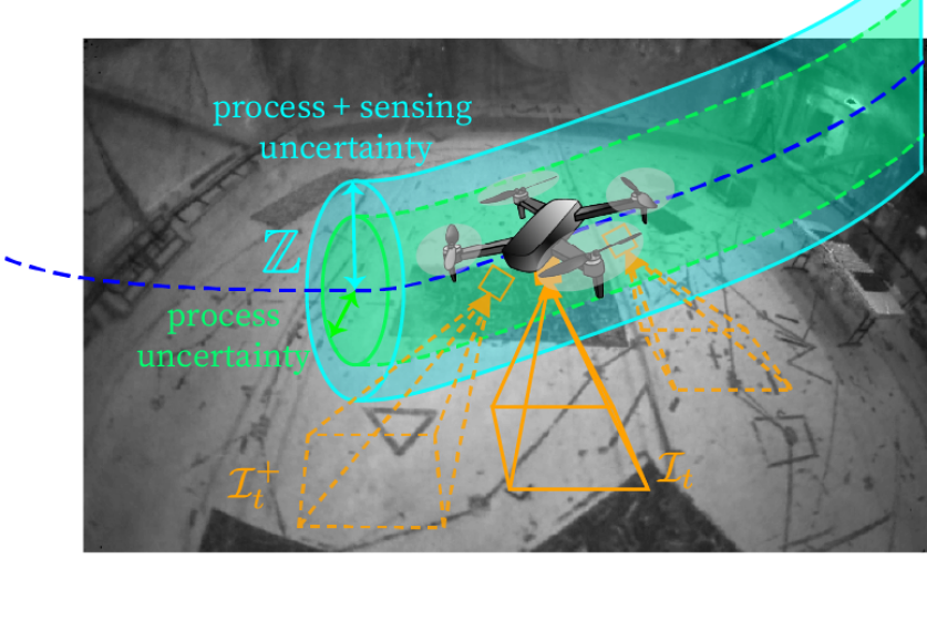
In this work, summarized in Figure 1, we propose Tube- Neural Radiance Field (NeRF), a new DA framework that enables efficient learning of robust visuomotor policies from MPC and that overcomes the aforementioned limitations in DA. Tube-NeRF extends our previous DA strategy for IL [9], where we showed that a robust variant of MPC, robust tube model predictive controller (RTMPC) [22], can be used to efficiently and systematically generate extra data for sample-efficient learning of motor control policies (e.g., actions from full state). The new work presented herein enables efficient learning of policies that directly use vision and other sensors as input, relaxing the constraining assumption in our previous work [9] that full-state information is available at deployment.

Our new strategy first collects robust task-demonstrations that account for the effects of process and sensing uncertainties via an output-feedback variant of RTMPC [23]. Then, we employ a photorealistic representation of the environment, based on a NeRF, to generate novel views for DA, using the tube of the controller to guide the selection of the extra novel views and sensorial inputs, and using the ancillary controller to efficiently compute the corresponding actions. We further enhance DA by organizing collected real-world observations in a database and employing the tube to generate queries. This enables usage of real-world data for DA, reducing the sim-to-real gap when only synthetic images are used. Lastly, we adapt our approach to a multirotor, training a visuomotor policy for robust trajectory tracking and localization using onboard camera images and additional measurements of altitude, orientation, and velocity. The generated policy relies solely on images to obtain information on the robot’s horizontal position, which is a challenging task due to (1) its high speed (up to $3.5$ m/s), (2) varying altitude, (3) aggressive roll/pitch changes, (4) the sparsity of visual features in our flight space, and (5) the presence of a safety net that moves due to the down-wash of the propellers and that produces semi-transparent visual features above the ground.

This Letter is an evolution of our previous conference paper [24], where we demonstrated the capabilities of our framework in simulation. In this extension, (i) we present the first-ever real-time deployment of our approach, demonstrating (in more than $30$ flights) successful agile trajectory tracking with policies that use onboard camera images to infer the horizontal position of a multirotor despite aggressive 3D motion, and subject to a variety of sensing and dynamics disturbances. Our policy has an average inference time of only $1.5$ ms onboard a small GPU (Nvidia Jetson TX2) and is deployed at $200$ Hz. To achieve these results, we (ii) leverage a NeRF instead of 3D meshes (as in [24]) for photo-realistic novel view-synthesis for DA; (iii) modify our DA strategy to include real-world images during DA, further reducing the sim-to-real gap in the deployment of our policies, (iv) employ a computationally-efficient but capable visuomotor NN architecture for onboard deployment, and (v) use randomization in image space to increase robustness to visual changes in the environment.

Contributions:

1. A new DA strategy enabling efficient (demonstrations, training time) learning of a sensorimotor policy from MPC. The policy generates actions using raw images and other measurements, instead of the full-state estimate [9], and is robust in the real world to a variety of uncertainties. Our approach is grounded in the output feedback RTMPC framework theory, unlike previous DA methods that rely on handcrafted heuristics, and uses a NeRF to generate images.

2. A procedure to apply our methodology for tracking and localization on a multirotor, using onboard images from a fisheye camera and altitude, attitude and velocity data.

3. Numerical and experimental evaluations of a policy learned from a single demonstration that runs onboard in $1.5$ ms on average under a variety of different uncertainties (wind, a slung-load causing visual disturbances, sensing noise).

II RELATED WORKS

Robust/efficient IL of sensorimotor policies. Table I presents state-of-the-art approaches for sensorimotor policy learning from demonstrations (from MPC or humans), focusing on mobile robots. DA-NeRF is the only method that (i) explicitly accounts for uncertainties, (ii) is efficient to train, and (iii) does not require visual abstractions (iv) nor specialized data collection setups. Related to our research, [21] employs a NeRF for DA from human demonstrations for manipulation, but uses heuristics to select relevant views, without explicitly accounting for uncertainties. Tube-NeRF uses properties of robust MPC to select relevant views and actions for DA, accounting for uncertainties. In addition, we incorporate available real-world images for DA, further reducing the sim-to-real gap.

TABLE I: Approaches that learn visuomotor policies from demonstrations. We highlight that (i) training the policy entirely in simulation often requires visual-abstractions for real-world deployments (e.g., [5]), losing however important information about the environment. Instead, approaches that directly use images (ii) benefit from data collection in the real-world, but require a large number of demonstrations (e.g., [6]), or (iii) leverage DA strategies that however use specialized data collection equipment and their deployment has been focused on ground robots (2D domain) ( [17, 19]) or to generate low-dimensional, discrete actions for aerial tasks (e.g., move left-right [18]). Additionally, all the considered DA approaches employ ad-hoc heuristics to select extra sensorial data and/or to compute the corresponding actions.

Method	Domain of training data	Policy directly uses images	Avoids specialized data-collection equipment	Demonstration-efficient	Explicitly accounts for uncertainties	Avoids Hand-Crafted Heuristics for Data Augm.	Real-world deployment (2D/3D, Domain)
[25] (MPC-GPS)	Sim.	Yes	Yes	No	No	N.A.	No (3D, Aerial)
[14] (PLATO)	Sim.	No	Yes	Yes	No	N.A.	No (3D, Aerial)
[20] (BC+DA)	Sim.	Yes	Yes	Yes	No	No	No (3D, Aerial)
[5] (DAgger+DR)	Sim	No	Yes	No	Yes	N.A.	Yes (3D, Aerial)
[6] (DAgger)	Real	Yes	Yes	No	No	N.A.	Yes (2D, Ground)
[19] (DAgger+DA)	Real	Yes	No	Yes	No	No	Yes (2D, Ground)
[17] (BC+DA)	Real	Yes	No	Yes	No	No	Yes (2D, Ground)
[18] (BC+DA)	Real	Yes	No	Yes	No	No	Yes (3D, Aerial)
[21] (SPARTAN)	Real	Yes	Yes	Yes	No	No	Yes (3D, Arm)
Tube-NeRF (proposed)	Real	Yes	Yes	Yes	Yes	Yes	Yes (3D, Aerial)

Novel view synthesis with NeRFs. NeRFs [26] enable efficient [27] and photorealistic novel view synthesis by directly optimizing the photometric accuracy of the reconstructed images, in contrast to traditional 3D photogrammetry methods (e.g., for 3D meshes). This provides accurate handling of transparency, reflective materials, and lighting conditions. Ref. [28] employs a NeRF to create a simulator for learning legged robot control policies from RGB images using Reinforcement Learning (RL). While they utilize a specialized camera for data collection, we use the same camera and we incorporate those images into the DA approach. Ref. [29] uses a NeRF for estimation, planning, and control on a drone by querying the NeRF online, but this results in $1000\times$ higher computation time than our policy.

Output feedback RTMPC. MPC [7] solves a constrained optimization problem that uses a model of the system dynamics to plan for actions that satisfy state and actuation constraints. Robust variants of MPC typically assume that the system is subject to additive, bounded process uncertainty (disturbances, model errors), and either a) plan by assuming a worst-case disturbance [30, 31], or b) employs an auxiliary (ancillary) controller, as in RTMPC, that maintains the system within some known distance (cross-section of a tube) of the plan [23]. Output feedback RTMPC [23, 32] in addition accounts for the effects of sensing uncertainty (noise, estimation errors) by increasing the cross-section of the tube. Our method uses an output-feedback RTMPC for data collection but bypasses its computational cost at deployment by learning a NN policy.

III PROBLEM FORMULATION

Our goal is to efficiently train a NN visuomotor policy $\pi_{\theta}$ (student), with parameters $\theta$, that tracks a desired trajectory on a mobile robot (e.g., multirotor). $\pi_{\theta}$ takes as input images, which are needed to extract partial state information (e.g., horizontal position), and other measurements. The trained policy, denoted $\pi_{\hat{\theta}^{*}}$, needs to be robust to uncertainties encountered in the deployment domain $\mathcal{T}$. It is trained using demonstrations from a model-based controller (expert) collected in a source domain $\mathcal{S}$ that presents only a subset of the uncertainties in $\mathcal{T}$.

Student policy. The student policy has the form:

$$\small\mathbf{u}_{t}=\pi_{\theta}(\mathbf{o}_{t},\mathbf{X}^{\text{des}}_{t}),$$ (1)

and it generates deterministic, continuous actions $\mathbf{u}_{t}$ to track a desired $N+1$ steps ($N>0$) trajectory $\mathbf{X}^{\text{des}}_{t}=\{\mathbf{x}^{\text{des}}_{0|t},\dots,\mathbf{x}^{\text{des}}_{N|t}\}$. $\mathbf{o}_{t}=(\mathcal{I}_{t},\mathbf{o}_{\text{other},t})$ are noisy sensor measurements comprised of an image $\mathcal{I}_{t}$ from an onboard camera, and other measurements $\mathbf{o}_{\text{other,t}}$ (e.g., altitude, attitude, velocity).

Expert. Process model: The dynamics of the robot are described by (e.g., via linearization):

$$\small\mathbf{x}_{t+1}=\mathbf{A}\mathbf{x}_{t}+\mathbf{B}\mathbf{u}_{t}+\mathbf{w}_{t}\\$$ (2)

where $\mathbf{x}_{t}\in\mathbb{X}\subset\mathfrak{R}^{n_{x}}$ is the state, and $\mathbf{u}_{t}\in\mathbb{U}\subset\mathfrak{R}^{n_{u}}$ the control inputs. The robot is subject to state and input constraints $\mathbb{X}$ and $\mathbb{U}$, assumed convex polytopes containing the origin [23]. $\mathbf{w}_{t}\in\mathbb{W}_{\mathcal{T}}\subset\mathfrak{R}^{n_{x}}$ in (2) captures time-varying additive process uncertainties in $\mathcal{T}$, such as (i) disturbances (e.g., wind for a UAV) (ii) and model changes/errors (e.g., linearization, discretization, and poorly known parameters). $\mathbf{w}_{t}$ is unknown, but the polytopic bounded set $\mathbb{W}_{\mathcal{T}}$ is assumed known[23]. Sensing model: The expert has access to (i) the measurements $\mathbf{o}_{\text{other},t}$, and (ii) a vision-based position estimator $g_{\text{cam}}$ (e.g., via SLAM) that outputs noisy measurements $\mathbf{o}_{\text{pos.xy}}\in\mathfrak{R}^{2}$ of the horizontal position $\bm{p}_{{xy},t}\in\mathfrak{R}^{2}$ of the robot:

$$\mathbf{o}_{\text{pos,xy},t}=g_{\text{cam}}(\mathcal{I}_{t})=\bm{p}_{{xy},t}+\mathbf{v}_{\text{\text{cam}},t},$$ (3)

where $\mathbf{v}_{\text{cam},t}$ is the associated sensing uncertainty. The measurements available to the expert are denoted $\bar{\mathbf{o}}_{t}\in\mathfrak{R}^{n_{o}}$, and they map to the robot state via:

$$\small\bar{\mathbf{o}}_{t}=\begin{bmatrix}\mathbf{o}_{\text{pos.xy},t}^{T},\mathbf{o}_{\text{other},t}^{T}\end{bmatrix}^{T}=\mathbf{C}\mathbf{x}_{t}+\mathbf{v}_{t},$$ (4)

where $\mathbf{C}\in\mathfrak{R}^{n_{o}\times n_{x}}$. $\mathbf{v}_{t}=[\mathbf{v}_{\text{\text{cam}},t}^{T},\mathbf{v}_{\text{other},t}^{T}]^{T}\in\mathbb{V}_{\mathcal{T}}\subset\mathfrak{R}^{n_{o}}$ is additive sensing uncertainty (e.g., noise, biases) in $\mathcal{T}$. $\mathbb{V}_{\mathcal{T}}$ is a known bounded set obtained via system identification, and/or via prior knowledge on the accuracy of $g_{\text{cam}}$.

State estimator. We assume the expert uses a state estimator:

$$\small\hat{\mathbf{x}}_{t+1}=\mathbf{A}\hat{\mathbf{x}}_{t}+\mathbf{B}\mathbf{u}_{t}+\mathbf{L}(\bar{\mathbf{o}}_{t}-\hat{\mathbf{o}}_{t}),\quad\hat{\mathbf{o}}_{t}=\mathbf{C}\hat{\mathbf{x}}_{t},$$ (5)

where $\hat{\mathbf{x}}_{t}\in\mathfrak{R}^{n_{x}}$ is the estimated state, and $\mathbf{L}\in\mathfrak{R}^{n_{x}\times n_{o}}$ is the observer gain, set so that $\mathbf{A}-\mathbf{L}\mathbf{C}$ is Schur stable. The observability index of the system $(\mathbf{A},\mathbf{C})$ is assumed to be $1$, meaning that full state information can be retrieved from a single noisy measurement. In this case, the observer plays the critical role of filtering out the effects of noise and sensing uncertainties. Additionally, we assume that the state estimation dynamics and noise sensitivity of the learned policy will approximately match the ones of the observer.

IV METHODOLOGY

Overview. Tube-NeRF collects trajectory tracking demonstrations in the source domain $\mathcal{S}$ using an output feedback RTMPC expert combined with a state estimator Eq. 5, and IL methods (DAgger or BC). The chosen output feedback RTMPC framework is based on [23, 32], with its objective function modified to track a trajectory (Section IV-A), and is designed according to the priors on process and sensing uncertainties at deployment ($\mathcal{T}$). Then, Tube-NeRF uses properties of the expert to design an efficient DA strategy, the key to overcoming efficiency and robustness challenges in IL (Section IV-B). The framework is then tailored to a multirotor leveraging a NeRF as part of the proposed DA strategy (Section V).

IV-A Output feedback robust tube MPC for trajectory tracking

Output feedback RTMPC for trajectory tracking regulates the system in Eq. 2 and Eq. 5 along a given reference trajectory $\mathbf{X}^{\text{des}}_{t}$, while satisfying state and actuation constraints $\mathbb{X},\mathbb{U}$ regardless of sensing uncertainties ($\mathbf{v}$, Eq. 4) and process noise ($\mathbf{w}$, Eq. 2).

Preliminary (set operations): Given the convex polytopes $\mathbb{A}\subset\mathfrak{R}^{n},\mathbb{B}\subset\mathfrak{R}^{n}$ and $\mathbf{M}\in\mathfrak{R}^{m\times n}$, we define:

• Minkowski sum: $\mathbb{A}\oplus\mathbb{B}\coloneqq\{\mathbf{a}+\mathbf{b}\in\mathfrak{R}^{n}\>|\>\mathbf{a}\in\mathbb{A},\>\mathbf{b}\in\mathbb{B}\}$

• Pontryagin diff.: $\mathbb{A}\ominus\mathbb{B}\coloneqq\{\mathbf{c}\in\mathfrak{R}^{n}\>|\>\mathbf{c+b}\in\mathbb{A},\forall\mathbf{b}\in\mathbb{B}\}$

• Linear mapping: $\mathbf{M}\mathbb{A}\coloneqq\{\mathbf{M}\mathbf{a}\in\mathfrak{R}^{m}\>|\>\mathbf{a}\in\mathbb{A}\}$.

Optimization problem. At every timestep $t$, RTMPC solves:

$$\small\begin{split}\mathbf{\bar{U}}_{t}^{*},\mathbf{\bar{X}}_{t}^{*}=\underset{\mathbf{\bar{U}}_{t},\mathbf{\bar{X}}_{t}}{\text{argmin}}&\|\mathbf{e}_{N|t}\|^{2}_{\mathbf{P}}+\sum_{i=0}^{N-1}\|\mathbf{e}_{i|t}\|^{2}_{\mathbf{Q}}+\|\mathbf{u}_{i|t}\|^{2}_{\mathbf{R}}\\ \text{subject to}\>\>&\bar{\mathbf{x}}_{i+1|t}=\mathbf{A}\bar{\mathbf{x}}_{i|t}+\mathbf{B}\bar{\mathbf{u}}_{i|t},\>\>i=0,\dots,N-1\\ &\bar{\mathbf{x}}_{i|t}\in\bar{\mathbb{X}},\>\>\bar{\mathbf{u}}_{i|t}\in\bar{\mathbb{U}},\\ &\mathbf{\bar{x}}_{N|t}\in\bar{\mathbb{X}}_{N},\>\>\hat{\mathbf{x}}_{t}\in\bar{\mathbf{x}}_{0|t}\oplus\begin{bmatrix}\bm{0}_{n_{x}},\!\!\!\!&\!\!\!\bm{I}_{n_{x}}\\ \end{bmatrix}\mathbb{S},\\ \end{split}$$ (6)

where $\mathbf{e}_{i|t}=\bar{\mathbf{x}}_{i|t}-\mathbf{x}^{\text{des}}_{i|t}$ represents the trajectory tracking error, $\mathbf{\bar{X}}_{t}=\{\bar{\mathbf{x}}_{0|t},\dots,\bar{\mathbf{x}}_{N|t}\}$ and $\mathbf{\bar{U}}_{t}=\{\bar{\mathbf{u}}_{0|t},\dots,\bar{\mathbf{u}}_{N-1|t}\}$ are safe reference state and action trajectories, and $N+1$ is the length of the planning horizon. The positive semi-definite matrices $\mathbf{Q}$ (size $n_{x}\times n_{x}$) and $\mathbf{R}$ (size $n_{u}\times n_{u}$) are tuning parameters, $\|\mathbf{e}_{N|t}\|^{2}_{\mathbf{P}}$ is a terminal cost (obtained by solving the infinite-horizon optimal control problem with $\mathbf{A}$, $\mathbf{B}$, $\mathbf{Q}$, $\mathbf{R}$) and $\mathbf{\bar{x}}_{N|t}\in\bar{\mathbb{X}}_{N}$ is a terminal state constraint.

Ancillary controller. The control input $\mathbf{u}_{t}$ is obtained via:

$$\small\mathbf{u}_{t}=\mathbf{\bar{\mathbf{u}}}^{*}_{t}+\mathbf{K}(\hat{\mathbf{x}}_{t}-\bar{\mathbf{x}}^{*}_{t}),$$ (7)

where $\bar{\mathbf{u}}^{*}_{t}\coloneqq\bar{\mathbf{u}}^{*}_{0|t}$ and $\bar{\mathbf{x}}^{*}_{t}\coloneqq\bar{\mathbf{x}}^{*}_{0|t}$, and $\mathbf{K}$ is computed by solving the LQR problem with $\mathbf{A}$, $\mathbf{B}$, $\mathbf{Q}$, $\mathbf{R}$. This controller maintains the system inside a set $\mathbb{Z}\oplus\bar{\mathbf{x}}_{t}^{*}$ (“cross-section” of a tube centered around $\bar{\mathbf{x}}_{t}^{*}$), regardless of the uncertainties.

Tube and robust constraints. Process and sensing uncertainties are taken into account by tightening the constraints $\mathbb{X}$, $\mathbb{U}$, obtaining $\bar{\mathbb{X}}$ and $\bar{\mathbb{U}}$ in Eq. 6. The amount by which $\mathbb{X}$, $\mathbb{U}$ are tightened depends on the cross-section of the tube $\mathbb{Z}$, which is computed by observing that the ancillary controller Eq. 7 combined with the system dynamics in Eq. 2 and the observer Eq. 5 constitute a closed-loop system. Sensing uncertainties in $\mathbb{V}_{\mathcal{T}}$ and process noise in $\mathbb{W}_{\mathcal{T}}$ introduce two sources of errors in such system: a) the state estimation error $\bm{\xi}^{\text{est}}_{t}\coloneqq\mathbf{x}_{t}-\hat{\mathbf{x}}_{t}$, and b) the control error $\bm{\xi}^{\text{ctrl}}_{t}\coloneqq\hat{\mathbf{x}}_{t}-\bar{\mathbf{x}}_{t}^{*}$. These errors can be combined in a vector $\bm{\xi}_{t}=[{\bm{\xi}^{\text{est}}_{t}}^{T},{\bm{\xi}^{\text{ctrl}}_{t}}^{T}]^{T}$ whose dynamics evolve according to (see [33, 32]):

$$\small\bm{\xi}_{t+1}=\mathbf{A}_{\xi}\bm{\xi}_{t}+\bm{\delta}_{t},\;\bm{\delta}_{t}\in\mathbb{D}\\$$ (8)

$$\small\mathbf{A}_{\xi}=\begin{bmatrix}\mathbf{A}-\mathbf{L}\mathbf{C}&\mathbf{0}_{n_{x}}\\ \mathbf{L}\mathbf{C}&\mathbf{A}+\mathbf{B}\mathbf{K}\end{bmatrix},\quad\mathbb{D}=\begin{bmatrix}\mathbf{I}_{n_{x}}&-\mathbf{L}\\ \mathbf{0}_{n_{x}}&\mathbf{L}\end{bmatrix}\begin{bmatrix}\mathbb{W}_{\mathcal{T}}\\ \mathbb{V}_{\mathcal{T}}\end{bmatrix}.$$

By design, $\mathbf{A}_{\xi}$ is a Schur-stable dynamic system, and it is subject to uncertainties from the convex polytope $\mathbb{D}$. Then, it is possible to compute the minimal Robust Positive Invariant (RPI) set $\mathbb{S}$, that is the smallest set satisfying:

$$\small\bm{\xi}_{0}\in\mathbb{S}\implies\bm{\xi}_{t}\in\mathbb{S},\;\forall\;\bm{\delta}_{t}\in\mathbb{D},\;t>0.$$ (9)

$\mathbb{S}$ represents the possible set of state estimation and control errors caused by uncertainties and is used to compute $\bar{\mathbb{X}}$ and $\bar{\mathbb{U}}$. Specifically, the error between the true state $\mathbf{x}_{t}$ and the reference state $\bar{\mathbf{x}}_{t}^{*}$ is: $\bm{\xi}^{\text{tot}}\coloneqq\mathbf{x}_{t}-\bar{\mathbf{x}}_{t}^{*}=\bm{\xi}^{\text{ctrl}}+\bm{\xi}^{\text{est}}.$ As a consequence, the effects of noise and uncertainties can be taken into account by tightening the constraints of an amount:

$$\small\bar{\mathbb{X}}\coloneqq\mathbb{X}\ominus\mathbb{Z},\;\mathbb{Z}=\begin{bmatrix}\bm{I}_{n_{x}}&\bm{I}_{n_{x}}\\ \end{bmatrix}\mathbb{S},\quad\bar{\mathbb{U}}\coloneqq\mathbb{U}\ominus\begin{bmatrix}\bm{0}_{n_{x}}&\mathbf{K}\end{bmatrix}\mathbb{S}.$$ (10)

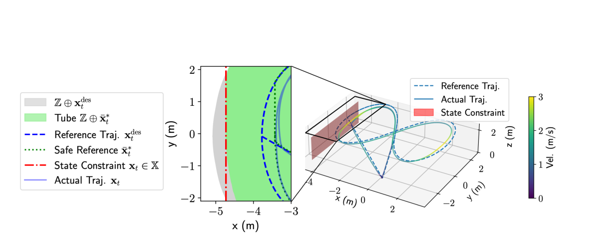
$\mathbb{Z}$ (cross-section of a tube) is the set of possible deviations of the true state $\mathbf{x}_{t}$ from the safe reference $\bar{\mathbf{x}}_{t}^{*}$. Figure 2 shows an example of this controller for trajectory tracking on a multirotor, highlighting changes to the reference trajectory to respect state constraint under uncertainties.

Figure 2: Output feedback RTMPC generates and tracks a safe reference to satisfy constraints.

IV-B Tube-guided DA for visuomotor learning

IL objective. We denote the expert output feedback RTMPC in Eq. 6, Eq. 7 and the state observer in Eq. 5 as $\pi_{\theta^{*}}$. The goal is to design an IL and DA strategy to efficiently learn the parameters $\hat{\theta}^{*}$ of the policy Eq. 1, collecting demonstrations from the expert $\pi_{\theta^{*}}$. In IL, this objective is achieved by solving:

$$\small\hat{\theta}^{*}\in\text{arg}\min_{\theta}\mathbb{E}_{p(\tau|\pi_{\theta},\mathcal{T})}[J(\theta,\theta^{*}|\tau)],$$ (11)

where $J$ is a distance metric, chosen to be the MSE loss:

$$\small J(\theta,\theta^{*}|\tau)=\frac{1}{T}\sum_{t=0}^{T-1}\|\pi_{\theta}(\mathbf{o}_{t},\mathbf{X}_{t}^{\text{des}})-\pi_{\theta^{*}}(\mathbf{o}_{t},\mathbf{X}_{t}^{\text{des}})\|_{2}^{2},$$ (12)

and $\tau:=\{(\mathbf{o}_{t},\mathbf{u}_{t},\mathbf{X}^{\text{des}}_{t})\!\mid\!\!t\!=\!0,\!\dots,\!T\}$ is a $T+1$ step (observation, action, reference) trajectory sampled from the distribution $p(\tau|\pi_{\theta},\mathcal{T})$. Such a distribution represents all the possible trajectories induced by the student policy $\pi_{\theta}$ in the deployment environment $\mathcal{T}$. As observed in [8, 9], the presence of uncertainties in $\mathcal{T}$ makes IL challenging, as demonstrations are usually collected in a training domain ($\mathcal{S}$) under a different set of uncertainties ($\mathbb{W}_{\mathcal{S}}\subseteq\mathbb{W}_{\mathcal{T}}$, $\mathbb{V}_{\mathcal{S}}\subseteq\mathbb{V}_{\mathcal{T}}$) resulting in a different distribution of training data.

Tube and ancillary controller for DA. To overcome these limitations, we design a DA strategy that compensates for the effects of process and sensing uncertainties encountered in $\mathcal{T}$. We do so by extending our previous approach [9], named Sampling Augmentation (SA), which provided a strategy to efficiently learn a control policy (i.e., $\hat{\pi}:\mathfrak{R}^{n_{x}}\rightarrow\mathfrak{R}^{n_{u}}$) robust to process uncertainty ($\mathbb{W}_{\mathcal{T}}$). SA recognized that the tube in a RTMPC [22] represents a model of the states that the system may visit when subject to process uncertainties. SA used the tube in [22] to guide the selection of extra states for DA, while the ancillary controller in [22] provided a computationally efficient way to compute corresponding actions, maintaining the system inside the tube for every possible realization of the process uncertainty.

Tube-NeRF. Our new approach, named Tube-NeRF, employs the output feedback variant of RTMPC presented in Section IV-A. This has two benefits: (i) the controller appropriately introduces extra conservativeness during demonstration collection to account for sensing uncertainties (via tightened constraint $\bar{\mathbb{X}}$ and $\bar{\mathbb{U}}$ in Eq. 6); and (ii) the tube $\mathbb{Z}$ in Eq. 10 additionally captures the effects of sensing uncertainty, guiding the generation of extra observations for DA. The new data collection and DA procedure is as follows.

IV-B1 Demonstration collection

We collect demonstrations in $\mathcal{S}$ using the output feedback RTMPC expert (Section IV-A). Each $T+1$-step demonstration $\bar{\tau}$ consists of:

$$\small\bar{\tau}=\{(\mathbf{o}_{t},\mathbf{u}_{t},\bar{\mathbf{u}}_{t}^{*},\bar{\mathbf{x}}_{t}^{*},\mathbf{X}^{\text{des}}_{t},\hat{\mathbf{x}}_{t})\mid t=0,\dots,T\}.$$ (13)

IV-B2 Extra states and actions for synthetic data generation

For every timestep $t$ in $\bar{\tau}$, we generate $N_{\text{synthetic},t}>0$ (details on how $N_{\text{synthetic},t}$ is computed are provided in Section IV-B4) extra (state, action) pairs $(\mathbf{x}_{t,j}^{+},\mathbf{u}_{t,j}^{+})$, with $j=1,\dots,N_{\text{synthetic},t}$ by sampling extra states from the tube $\mathbf{x}_{t,j}^{+}\in\bar{\mathbf{x}}_{t}^{*}\oplus\mathbb{Z}$, and computing the corresponding control action $\mathbf{u}_{t,j}^{+}$ using the ancillary controller Eq. 7:

$$\small\mathbf{u}_{t,j}^{+}=\mathbf{\bar{\mathbf{u}}}_{t}^{*}+\mathbf{K}(\mathbf{x}_{t,j}^{+}-\bar{\mathbf{x}}_{t}^{*}).$$ (14)

The resulting $\mathbf{u}_{t,j}^{+}$ is saturated to ensure that $\mathbf{u}_{t,j}^{+}\in\mathbb{U}$.

IV-B3 Synthetic observations generation

To generate the necessary data $\mathbf{o}_{t,j}^{+}=(\mathcal{I}_{t,j}^{+},\mathbf{o}_{\text{other},{t,j}}^{+})$ input for the sensorimotor policy Eq. 1 from the selected states $\mathbf{x}_{j,t}^{+}$, we employ observation models Eq. 4 available for the expert. In the context of learning a visuomotor policy, we generate synthetic camera images $\mathcal{I}_{t,j}^{+}$ using an inverse pose estimator $\hat{g}^{-1}_{\text{\text{cam}}}$, mapping camera poses $\mathbf{T}_{IC}$ to images $\mathcal{I}$ via $\small\mathcal{I}_{t,j}^{+}=\hat{g}_{\text{\text{cam}}}^{-1}(\mathbf{T}_{{IC}_{t,j}}^{+}),$ where $\mathbf{T}_{IC}$ denotes a homogeneous transformation matrix from a world (inertial) frame $I$ to a camera frame $C$. $\hat{g}^{-1}_{\text{\text{cam}}}$ is obtained by generating a NeRF of the environment (discussed in more details in Section V-1) from the images $\mathcal{I}_{0},\dots,\mathcal{I}_{T}$ in the collected demonstration $\bar{\tau}$, and by estimating the intrinsic/extrinsic of the camera onboard the robot. The camera poses $\textbf{T}_{{IC}_{t,j}}^{+}$ are obtained from the sampled states $\mathbf{x}_{t,j}^{+}$, which includes the robot’s position and orientation. These are computed as $\textbf{T}_{{IC}_{t,j}}^{+}=\textbf{T}_{IB}(\mathbf{x}_{t,j}^{+})\hat{\textbf{T}}_{{BC}_{t,j}}$, where $\textbf{T}_{IB}$ is the transformation from the robot’s body frame $B$ to the reference frame $I$, and $\hat{\textbf{T}}_{{BC}_{t,j}}$ is the perturbed transformation between $B$ and the camera frame $C$. Perturbations in $\hat{\textbf{T}}_{{BC}_{t,j}}$, applied to the camera’s nominal extrinsic $\textbf{T}_{BC}$, accommodate uncertainties and errors in the camera extrinsics. Last, the full observations $\mathbf{o}_{t,j}^{+}$ are obtained by computing $\mathbf{o}_{\text{other},t,j}^{+}$, using Eq. 4 and a selection matrix $\mathbf{S}$:

$$\small\mathbf{o}_{t,j}^{+}=(\mathcal{I}_{t,j}^{+},\mathbf{o}_{\text{other},t,j}^{+}),\;\;\mathbf{o}_{\text{other},t,j}^{+}=\mathbf{S}\mathbf{C}\mathbf{x}_{t,j}^{+}.$$ (15)

IV-B4 Tube-guided selection of extra real observations

Beyond guiding the generation of extra synthetic data, we employ the tube of the expert to guide the selection of real-world observations from demonstrations ($\bar{\tau}$) for DA. This procedure is useful at accounting for small imperfections in the NeRF and in the camera-to-robot extrinsic/intrinsic calibrations, further reducing the sim-to-real gap, and providing an avenue to “ground” the synthetic images with real-world data. This involves creating a database of the observations $\mathbf{o}$ in $\bar{\tau}$, indexed by the robot’s estimated state $\hat{\mathbf{x}}$, and then selecting $N_{\text{real},t}$ observations at each timestep $t$ inside the tube ($\hat{\mathbf{x}}\in\bar{\mathbf{x}}^{*}_{t}\oplus\mathbb{Z}$), adhering to the ratio $N_{\text{real},t}/N_{\text{samples}}\leq\bar{\epsilon}$, where $0<\bar{\epsilon}\leq 1$ is a user-defined parameter that balances the maximum ratio of real images to synthetic ones, and $N_{\text{samples}}$ is the desired number of samples (real and synthetic) per timestep. The corresponding action is obtained from the state associated with the image via the ancillary controller Eq. 14. The required quantity of synthetic samples to generate, as discussed in Section IV-B3, is calculated using the formula $N_{\text{synthetic},t}=N_{\text{samples}}-N_{\text{real},t}$.

IV-B5 Robustification to visual changes

To accommodate changes in brightness and environment, we apply several transformations to both real and synthetic images. These include solarization, adjustments in sharpness, brightness, and gamma, along with the application of Gaussian noise, Gaussian blur, and erasing patches of pixels using a rectangular mask.

V APPLICATION TO VISION-BASED FLIGHT

In this section, we provide details on the design of the expert, the student policy, and the NeRF for agile flight.

Figure 3: Architecture of the employed visuomotor student policy. The policy takes as input a raw camera image, a reference trajectory $\mathbf{x}^{\text{des}}_{0|t},\dots,\mathbf{x}^{\text{des}}_{N|t}$ and noisy measurements of the altitude $p^{m}_{z}$, velocity $\bm{v}_{t}$ and tilt (roll $\varphi_{t}$, pitch $\vartheta_{t}$) of the multirotor. It outputs an action $\textbf{u}_{t}$, representing a desired roll, pitch, and thrust set-points for the cascaded attitude controller. The policy additionally outputs an estimate of the state $\hat{\mathbf{x}}_{t}$, which was found useful to promote learning of features relevant to position estimation.

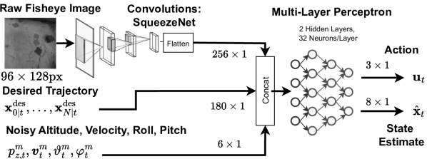
Task. We apply our framework to learn to track a figure-eight trajectory (lemniscate, with velocity up to $3.15$ m/s lasting $30$s), denoted T1. Robot model. The expert uses the hover-linearized model of a multirotor [34], with state $\mathbf{x}=[_{I}\bm{p}^{T},_{I}\bm{v}^{T},_{\bar{I}}\varphi,_{\bar{I}}\vartheta]^{T},$ (position $\bm{p}\in\mathfrak{R}^{3}$, velocity $\bm{v}\in\mathfrak{R}^{3}$, roll $\varphi\in\mathfrak{R}$, pitch $\vartheta\in\mathfrak{R}$, $n_{x}\!=\!8$), $I$ is an inertial reference frame, while ${\bar{I}}$ a yaw-fixed frame [34]. The control input $\mathbf{u}_{t}$ ($n_{u}\!=\!3$) is desired roll, pitch, and thrust, and it is executed by a cascaded attitude controller. Measurements. Our multirotor is equipped with a fisheye monocular camera, tilted $45\deg$ downwards, that generates images $\mathcal{I}_{t}$ (size $128\times 96$ pixels). In addition, we assume available onboard noisy altitude ${}_{I}p^{m}_{z}\in\mathfrak{R}$, velocity ${}_{I}\bm{v}^{m}\in\mathfrak{R}^{3}$ and roll ${}_{I}\varphi^{m}$, pitch ${}_{I}\vartheta^{m}$ and yaw measurements. This is a common setup in aerial robotics, where noisy altitude and velocity can be obtained, for example, via optical flow and a downward-facing lidar, while roll, pitch, and yaw can be computed from an IMU with a magnetometer, using a complementary filter [35]. Student policy. The student policy Eq. 1, whose architecture is shown in Figure 3, takes as input an image $\mathcal{I}_{t}$ from the onboard camera, the reference trajectory $\mathbf{X}^{\text{des}}_{t}$, and $\mathbf{o}_{\text{other}}\coloneqq[_{I}p^{m}_{z},{{}_{I}\bm{v}^{m}}^{T},_{\bar{I}}\varphi^{m},_{\bar{I}}\vartheta^{m}]^{T},$ and it outputs $\mathbf{u}_{t}$. A Squeezenet [36] is used to map $\mathcal{I}_{t}$ into a lower-dimensional feature space; it was selected for its performance at a low computational cost. To promote learning of internal features relevant to estimating the robot’s state, the output of the policy is augmented to predict the current state $\hat{\mathbf{x}}$ (or $\mathbf{x}^{+}$ for the augmented data), modifying Eq. 12 accordingly. This output was not used at deployment time, but it was found to improve the performance. Output Feedback RTMPC and observer. The expert uses the defined robot model for predictions, discretized with $T_{s}=0.1$ s, and horizon $N=30$, ($3.0$ s). $\mathbb{X}$ encodes safety and position limits, while $\mathbb{U}$ captures the maximum actuation capabilities. Process uncertainty in $\mathbb{W}_{\mathcal{T}}$ is assumed to be a bounded external force disturbance with magnitude up to $20\%$ of the weight of the robot and random direction, close to the physical limits of the platform. The state estimator Eq. 5 is designed by using as measurement model in Eq. 4: $\bar{\mathbf{o}}_{t}=\mathbf{x}_{t}+\mathbf{v}_{t}$ where we assume $\mathbf{v}_{t}\!\sim\!\mathcal{N}(\mathbf{0}_{n_{x}},[\bm{\sigma}^{T}_{\text{cam}},\bm{\sigma}^{T}_{\text{other}}]^{T})$. We therefore set $\mathbb{V}_{\mathcal{T}}=\{\mathbf{v}_{t}\;|\;\|\mathbf{v}\|_{\infty}\leq 3\left[\bm{\sigma}_{\text{cam}}^{T},\bm{\sigma}_{\text{other}}^{T}\right]^{T}\}$, with $3\bm{\sigma}_{\text{cam}}=[0.6,0.6]^{T}$ (units in $m$) and $3\bm{\sigma}_{\text{other}}=[0.4,0.2,0.2,0.2,0.05,0.05]^{T}$ (units in $m$ for altitude, $m/s$ for velocity, and $rad$ for tilt). These conservative but realistic parameters are based on prior knowledge of the worst-case performance of vision-based estimators in our relatively feature-poor flight space. The observer gain matrix $\mathbf{L}$ is computed by assuming fast state estimation dynamics, (poles of $\mathbf{A-LC}$ at $30.0$ rad/s). For simplicity, the RPI set $\mathbb{S}$ is obtained from $\mathbb{W}_{\mathcal{T}}$ and $\mathbb{V}_{\mathcal{T}}$ via Monte Carlo simulations of Eq. 8, uniformly sampling instances of the uncertainties, and by computing an outer axis-aligned bounding box of the trajectories of $\bm{\xi}$.

V-1 Procedure to generate the NeRF of the environment

(i) Dataset:A NeRF of the environment, the MIT-Highbay, is generated from about $100$ images collected during a single real-world demonstration of the figure-eight trajectory (T1) intended for learning, utilizing full-resolution images ($640\times 480$ pixels) from the fisheye camera onboard the Qualcomm Snapdragon Flight Pro board of our UAV. (ii) Extrinsic/Intrinsic:The extrinsic and intrinsic parameters of the camera are estimated from the dataset using structure-from-motion (COLMAP [37]). We chose the RADTAN camera model, as this was found to provide better reconstructions than higher-order fisheye models. (iii) Frame Alignment:The scale and homogeneous transformation aligning the reference frame used by the COLMAP with the reference frame used by the robot’s state estimator are determined via the trajectory alignment tool EVO [38]. This enables the integration of the NeRF as an image rendering tool in a simulation/DA framework. (iv) NeRF Training:Instant-NGP [27] is utilized to train the NeRF. The scaling of the Axis-Aligned Bounding Box used by the Instant-NGP is manually adjusted to ensure that the reconstruction is photorealistic in the largest possible volume. (v) Images rendering for DA:Novel images are rendered using the same camera intrinsics identified by COLMAP. The camera extrinsics, mapping from the robot’s IMU to the optical surface, are determined via Kalibr [39], using an ad-hoc dataset. An example of an image from the NeRF is shown in Figure 1.

VI Evaluation

VI-A Evaluation in simulation

Figure 4: Episode length (number of timestep before a state constraint violation, for a maximum of $300$ timesteps) as a function of the number of demonstrations collected from the expert, and as a function of the training time (the time required to collect such demonstrations in simulation, and to train the policy). Two deployment domains are considered, one with sensing noise and one with additional process noise (wind-like disturbances). The results highlight that policies trained with Tube-NeRF (TN) archive full episode length after a single demonstration, and require less than half of the training time than the best-performing baselines (DR-based methods). Reducing the number of samples extracted from the tube (e.g., TN-50) improves the training time. Note that the lines of Tube-NeRF-based approaches vs the number of demonstrations overlap. Shaded areas are $95\%$ confidence intervals. Note that to focus our study on the effects of process uncertainties and sensing noise, we do not apply visual changes to the environment, nor the robustification to visual changes (Section IV-B5). Evaluations across $10$ seeds.

TABLE II: robustness, performance, and demonstration efficiency of IL methods for visuomotor policy learning. An approach easy if it does not require disturbances during the demonstration collection, and it is safe if it does not violate state constraints (e.g., wall collision) during training. Success Rate is the percentage of trajectories that do no violate state constraints. Performance is the relative error between the cost of the trajectory generated by output feedback RTMPC (expert) and the ones from the policy. Demonstration efficiency is the number of demonstrations required to achieve at least $70\%$ success rate. Performance and robustness of the baselines are evaluated after $150$ demonstrations, while Tube-NeRF methods after only $2$ demonstrations.

Method		Training		Robustness succ. rate (%)		Performance expert gap (%)		Demonstration Efficiency
Robustif.	Imitation	Easy	Safe	Noise	Noise, Wind	Noise	Noise, Wind	Noise	Noise, Wind
-	BC	Yes	Yes	95.5	13.0	83.1	21.3	30	-
	DAgger	Yes	No	60.5	45.5	138.6	43.0	-	-
DR	BC	No	Yes	80.0	46.5	72.5	59.2	20	90
	DAgger	No	No	67.0	62.0	82.2	59.6	90	-
TN-100	BC	Yes	Yes	100.0	100.0	8.3	9.1	1	1
	DAgger	Yes	Yes	100.0	100.0	14.4	9.7	1	1
TN-50	BC	Yes	Yes	100.0	100.0	18.4	11.8	1	1
	DAgger	Yes	Yes	100.0	100.0	15.4	11.2	1	1

TABLE III: Position RMS Tracking Errors on the ${x,y,z}$ axis across multiple runs when following a figure-eight (lemniscate) trajectory (T1) and a circular trajectory (T2). These results highlight the overall low tracking errors of the sensorimotor policy, comparable to the ones of the expert whose position is estimated via a motion capture system. We apply wind disturbances with a leaf blower (With wind), and extra sensing noise in the altitude, velocity and orientation part input of the policy (High noise). Unlike in T1, the policy trained for T2 has been obtained without collecting corresponding images from a real-world demonstration, and therefore exclusively relies on the NeRF-based data augmentation during certain parts of the trajectory (see Figure 7). All experiments repeated $3$ times, except T2 with wind low noise (two times), and slung-load (once).

	RMSE (m, $\downarrow$) for T1: Lemniscate (30s, real-world demo.)							RMSE (m, $\downarrow$) for T2: Circle (30s, No real-world demo.)
	Expert + Motion Capture		Student					Student
	No wind	With wind	No wind		With wind		Slung load	No wind		With wind
	Low noise	Low noise	Low noise	High noise	Low noise	High noise		Low noise	High noise	Low noise	High noise
$x$	0.19 $\pm$ 0.00	0.20 $\pm$ 0.01	0.30 $\pm$ 0.01	0.33 $\pm$ 0.00	0.28 $\pm$ 0.02	0.40 $\pm$ 0.01	0.21	0.33 $\pm$ 0.01	0.34 $\pm$ 0.01	0.33 $\pm$ 0.00	0.34 $\pm$ 0.04
$y$	0.17 $\pm$ 0.01	0.21 $\pm$ 0.01	0.16 $\pm$ 0.01	0.21 $\pm$ 0.01	0.26 $\pm$ 0.01	0.22 $\pm$ 0.03	0.44	0.16 $\pm$ 0.01	0.27 $\pm$ 0.01	0.22 $\pm$ 0.03	0.28 $\pm$ 0.01
$z$	0.12 $\pm$ 0.01	0.13 $\pm$ 0.02	0.11 $\pm$ 0.01	0.20 $\pm$ 0.02	0.17 $\pm$ 0.01	0.17 $\pm$ 0.01	0.06	0.11 $\pm$ 0.08	0.15 $\pm$ 0.06	0.07 $\pm$ 0.00	0.14 $\pm$ 0.02

(a) T1, student w/o wind.

(b) T1, student w/ wind.

(c) T2, student w/o wind.

(d) T2, student w/ wind.

Figure 5: Qualitative evaluation of the trajectory tracking performance of the proposed sensorimotor policy, highlighting the high velocity and 3D motion of the robot, which in turn causes large roll/pitch changes. The eight-shaped trajectory (T1) is the same trajectory used to collect the real-world images and to generate the NeRF employed for Data Augmentation, while the circular trajectory is entirely trained without having collected in the real world a task demonstration. This demonstrates that our approach can be used to train vision-based policies (T2) for which no real-world demonstration has been collected, still achieving low tracking errors (comparable to T1).

Figure 6: Robustness of the policy to visual uncertainties: we show images captured by the onboard camera while using the proposed sensorimotor policy for localization and tracking of T1, with a slung load (tape roll, $0.2$ Kg) attached to the robot. The slung load (circled) repeatedly enters the field of view of the onboard camera, without however compromising the success of the maneuver. (Timestamp added in post-processing).

TABLE IV: Time (ms) required to generated a new action for the output feedback RTMPC only (Expert) and the proposed sensorimotor NN policy (Policy). Our policy is $\mathbf{9.8}$ faster (offboard) and $\mathbf{5.6}$ times faster (onboard) than the expert. We note that the computational cost of the expert is only based on computing actions from states, while the policy additionally performs localization (actions from images); therefore the reported data represents a lower bound on the cost reductions introduced by the policy. For a fair comparison, the onboard expert uses an highly-optimized C/C++ implementation. The offboard computer, used for our numerical evaluation and training, is an AMD Threadripper 3960X with two RTX 3090. The onboard implementation (optimized for speed for both the policy and the expert) uses an NVIDIA Jetson TX2.

			Time (ms)
Computer	Method	Setup	Mean	SD	Min	Max
Offboard	Expert (MPC only)	CVXPY/OSQP	$30.3$	$41.5$	$4.8$	$244.3$
	Policy (MPC+vision)	PyTorch	$\mathbf{3.1}$	$\mathbf{0.0}$	$\mathbf{0.8}$	$\mathbf{1.0}$
Onboard	Expert (MPC only)	CVXGEN	$8.4$	$1.4$	$4.5$	$15.9$
	Policy (MPC+vision)	ONNX/TensorRT	$\mathbf{1.5}$	$\mathbf{0.2}$	$\mathbf{1.4}$	$\mathbf{9.2}$

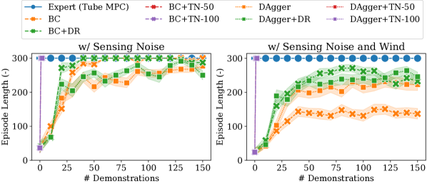
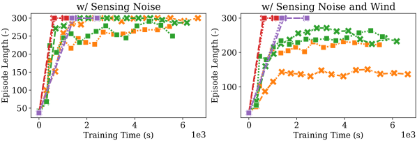
Here we numerically evaluate the efficiency (training time, number of demonstrations), robustness (average episode length before violating a state constraint, success rate) and performance (expert gap, the relative error between the stage cost $\sum_{t}\mathbf{\|}\mathbf{e}_{t}\|_{\mathbf{Q}}^{2}+\|\mathbf{u}_{t}\|^{2}_{\mathbf{R}}$ of the expert and the one of the policy) of Tube-NeRF. We use PyBullet to simulate realistic full nonlinear multirotor dynamics [34], rendering images using the NeRF obtained in Section V-1 – combined with realistic dynamics, the NeRF provides a convenient framework for training and numerical evaluations of policies. The considered task consists of following the figure-eight trajectory T1 (lemniscate, length: $300$ steps) used in Section V-1, starting from $\mathbf{x}_{0}\!\sim\!\text{Uniform}(-0.1,0.1)\in\mathbb{R}^{8}$, without violating state constraints. The policies are deployed in two target environments, one with sensing noise affecting the measurements $\mathbf{o}_{\text{other}}$ (the noise is Gaussian distributed with parameters as defined in Section V) and one that additionally presents wind disturbances, sampled from $\mathbb{W}_{\mathcal{T}}$ (also with bounds as defined in Section V). Method and baselines. We apply Tube-NeRF to BC and DAgger, comparing their performance without any DA; Tube-NeRF$-N_{\text{samples}}$, with $N_{\text{samples}}=\{50,100\}$, denotes the number of observation-action samples generated for every timestep by uniformly sampling states inside the tube. We additionally combine BC and DAgger with DR; in this case, during demonstration collection, we apply an external force disturbance (e.g., wind) sampled from $\mathbb{W}_{\mathcal{T}}$. We set $\beta$, the hyperparameter of DAgger controlling the probability of using actions from the expert instead of the learner policy, to be $\beta=1$ for the first set of demonstrations, and $\beta=0$ otherwise. Evaluation details. For every method, we: (i) collect $K$ new demonstrations ($K=1$ for Tube-NeRF, $K=10$ otherwise) via the output feedback RTMPC expert and the state estimator; (ii) update a student policy using all the demonstrations collected so far; (iii) evaluate the obtained policy in the considered target environments, for $10$ times each, starting from different initial states; (iv) repeat from (i). Results. The results are shown in Figure 4 and Table II. Figure 4 highlights that all Tube-NeRF methods, combined with either DAgger or BC, can achieve complete robustness (full episode length) under combined sensing and process uncertainties after a single demonstration. The baseline approaches require $20$-$30$ demonstrations to achieve a full episode length in the environment without wind, and the best-performing baselines (methods with DR) require about $80$ demonstrations to achieve their top episode length in the more challenging environment. Similarly, Tube-NeRF requires less than half training time than DR-based methods to achieve higher robustness in this more challenging environment, and reducing the number of samples (e.g, Tube-NeRF-$50$) can further improve the training time. Table II additionally highlights the small gap of Tube-NeRF policies from the expert in terms of tracking performance (expert gap), and shows that increasing the number of samples (e.g., Tube-NeRF-$100$) benefits performance.

VI-B Flight experiments

Figure 7: Number of real images sampled from the tube to perform data augmentation using Tube-NeRF-100, as a function of time in the considered trajectory. The considered trajectories are a Lemniscate trajectory (T1), which is the same as the one executed for real-world data collection, and a Circle trajectory (T2), which is different from the one executed for data collection. The results highlight that (1) the tube can be used to guide the selection of real-world images for data augmentation and (2) the synthetic images from the NeRF are a key component of our data augmentation strategy, as there are multiple segments of the circular trajectory (T2) where no real images are presents, but the sensorimotor policy successfully controls the robot in the real-world experiments.

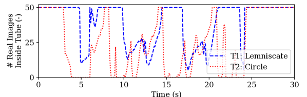
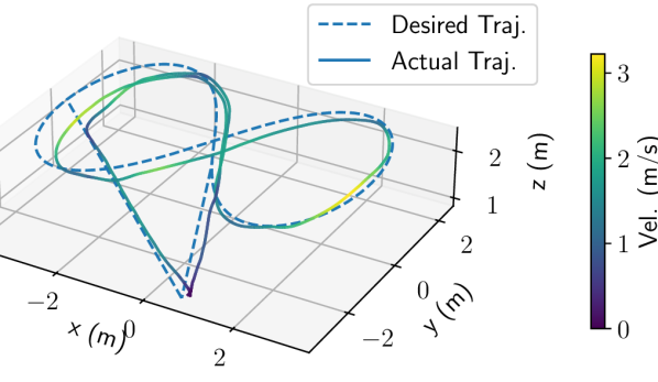
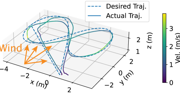
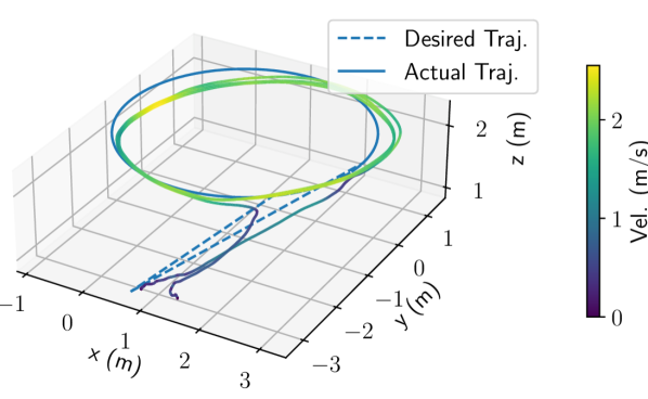
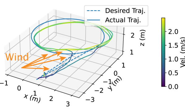
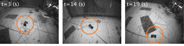
We now validate the data efficiency of Tube-NeRF highlighted in our numerical analysis by evaluating the obtained policies in real-world experiments. We do so by deploying them on an NVIDIA Jetson TX2 (at up to $200$ Hz, TensorRT) on the MIT-ACL multirotor. The policies take as input the fisheye images generated at $30$ or $60$ Hz by the onboard camera. The altitude, velocity and roll/pitch inputs that constitute $\textbf{o}_{\text{other},t}$ are, for simplicity, obtained from the onboard estimator (an EKF fusing IMU with poses from a motion capture system), corrupted with additive noise (zero-mean Gaussian, with parameters as defined in Section V) in the scenarios denoted as “high noise”. We remark that no information on the horizontal position of the UAV is provided to the policy, and horizontal localization must be performed from images. We consider two tasks, tracking the lemniscate trajectory (T1), and tracking a new circular trajectory (denoted T2, velocity up to $2.0$ m/s, duration of $30$ s). No real-world images have been collected for T2, therefore this task is useful to stress-test the novel-view synthesis abilities of the approach, using the NeRF and the nonlinear simulated robot dynamics as a simulation framework. Training. We train one policy for each task, using a single task demonstration collected with DAgger+Tube-NeRF-100 in our NeRF-based simulated environment. During DA, we try to achieve an equal amount between synthetic images (from the NeRF) and real ones (from the database), setting $\bar{\epsilon}=0.5$. Figure 7 reports the number of sampled real images from the database, highlighting that the tube is useful at guiding the selection of real images, but that synthetic images are a key part of the DA strategy (e.g., T2 presents multiple parts without any real image available). Performance under uncertainties. Figure 5 and Table III show the trajectory tracking performance of the learned policy under a variety of real-world uncertainties. Those uncertainties include (i) model errors, such as poorly known drag and thrust to voltage mappings; (ii) wind disturbances, applied via a leaf-blower, (iii) sensing uncertainties (additive Gaussian noise), and (iv) visual uncertainties, produced by attaching a slung-load that repeatedly enters the field of view of the camera, as shown in Figure 6. These results highlight that (a) policies trained after a single demonstration collected in our NeRF-based simulator using Tube-NeRF are robust to a variety of uncertainties while maintaining tracking errors comparable to the ones of the expert (Table III, Figure 2), while reaching velocities up to $3.5$ m/s, and even though the expert localizes using a motion capture system, while the policy uses images from the onboard camera to obtain its horizontal position. In addition, (b) our method enables learning of vision-based policies for which no real-world task demonstration has been collected (e.g., effectively acting as a simulation framework), as shown by the successful tracking of T2, which relied entirely on synthetic training data for large portions of the trajectory (Figure 7), and was obtained using a single demonstration in the NeRF-based simulator. Due to the limited robustness achieved in simulation (Table II), we do not deploy the baselines on the real robot. Efficiency at deployment. Table IV shows that onboard the policy requires on average only 1.5 ms to compute a new action from an image, being at least $\mathbf{5.6}$ faster than a highly-optimized (C/C++) expert. Note that the reported computational cost of the expert is based on the cost of control only (no state estimation), therefore the actual computational cost reduction provided by the policy is even larger.

VII DISCUSSION AND CONCLUSIONS

We have presented Tube-NeRF, a strategy for efficient IL of robust visuomotor policies. Tube-NeRF leverages a robust controller, output feedback RTMPC, to collect demonstrations that account for process and sensing uncertainties. The tube of the controller additionally guides the selection of relevant sensorial observations for DA —considering the effects of sensing noise, domain uncertainties, and disturbances. Extra observations are obtained via a database of real-world data and a NeRF of the environment, while the corresponding actions are efficiently computed using an ancillary controller. We have tailored our approach to localization and control of an aerial robot, showing in numerical evaluations that Tube-NeRF can learn a robust visuomotor policy from a single demonstration, outperforming IL baselines in demonstration and computational efficiency. Our experiments have validated the numerical finding, achieving accurate trajectory tracking using an onboard policy ($1.5$ ms average inference time) that relied entirely on images to infer the horizontal position of the robot, despite challenging 3D motion and uncertainties. In future work, we aim to harness the robustness and efficiency of our policies for localization and control onboard highly agile, computationally constrained, sub-gram aerial robots [40].

VIII ACKNOWLEDGMENTS

Victor D. Li and Tong Zhao for their help with the experiments. Xiaoyi (Jeremy) Cai for the feedback on the manuscript.

References

- [1] D. A. Pomerleau, “Alvinn: An autonomous land vehicle in a neural network,” Carnegie-Mellon Univ Pittsburgh PA Artificial Intelligence and Psychology, Tech. Rep., 1989.
- [2] B. D. Argall, S. Chernova, M. Veloso, and B. Browning, “A survey of robot learning from demonstration,” Robotics and autonomous systems, vol. 57, no. 5, pp. 469–483, 2009.
- [3] S. Ross, G. Gordon, and D. Bagnell, “A reduction of imitation learning and structured prediction to no-regret online learning,” in Proceedings of the fourteenth international conference on artificial intelligence and statistics. JMLR Workshop and Conference Proceedings, 2011, pp. 627–635.
- [4] A. Loquercio, E. Kaufmann, R. Ranftl, A. Dosovitskiy, V. Koltun, and D. Scaramuzza, “Deep drone racing: From simulation to reality with domain randomization,” IEEE Transactions on Robotics, vol. 36, no. 1, pp. 1–14, 2019.
- [5] E. Kaufmann, A. Loquercio, R. Ranftl, M. Müller, V. Koltun, and D. Scaramuzza, “Deep drone acrobatics,” Robotics, Science, and Systems (RSS), 2020.
- [6] Y. Pan, C.-A. Cheng, K. Saigol, K. Lee, X. Yan, E. A. Theodorou, and B. Boots, “Imitation learning for agile autonomous driving,” The International Journal of Robotics Research, vol. 39, no. 2-3, pp. 286–302, 2020.
- [7] F. Borrelli, A. Bemporad, and M. Morari, Predictive control for linear and hybrid systems. Cambridge University Press, 2017.
- [8] M. Laskey, J. Lee, R. Fox, A. Dragan, and K. Goldberg, “Dart: Noise injection for robust imitation learning,” in Conference on robot learning. PMLR, 2017, pp. 143–156.
- [9] A. Tagliabue, D.-K. Kim, M. Everett, and J. P. How, “Demonstration-efficient guided policy search via imitation of robust tube mpc,” in 2022 International Conference on Robotics and Automation (ICRA), 2022, pp. 462–468.
- [10] X. B. Peng, M. Andrychowicz, W. Zaremba, and P. Abbeel, “Sim-to-real transfer of robotic control with dynamics randomization,” in 2018 IEEE international conference on robotics and automation (ICRA). IEEE, 2018, pp. 3803–3810.
- [11] J. Tobin, R. Fong, A. Ray, J. Schneider, W. Zaremba, and P. Abbeel, “Domain randomization for transferring deep neural networks from simulation to the real world,” in 2017 IEEE/RSJ international conference on intelligent robots and systems (IROS). IEEE, 2017, pp. 23–30.
- [12] F. Sadeghi and S. Levine, “Cad2rl: Real single-image flight without a single real image,” Robotics, Science, and Systems (RSS), 2017.
- [13] A. Loquercio, E. Kaufmann, R. Ranftl, M. Müller, V. Koltun, and D. Scaramuzza, “Learning high-speed flight in the wild,” Science Robotics, vol. 6, no. 59, p. eabg5810, 2021.
- [14] G. Kahn, T. Zhang, S. Levine, and P. Abbeel, “Plato: Policy learning using adaptive trajectory optimization,” in 2017 IEEE International Conference on Robotics and Automation (ICRA). IEEE, 2017, pp. 3342–3349.
- [15] K. Lee, B. Vlahov, J. Gibson, J. M. Rehg, and E. A. Theodorou, “Approximate inverse reinforcement learning from vision-based imitation learning,” in 2021 IEEE International Conference on Robotics and Automation (ICRA), 2021, pp. 10 793–10 799.
- [16] R. Bonatti, R. Madaan, V. Vineet, S. Scherer, and A. Kapoor, “Learning visuomotor policies for aerial navigation using cross-modal representations,” in 2020 IEEE/RSJ International Conference on Intelligent Robots and Systems (IROS). IEEE, 2020, pp. 1637–1644.
- [17] M. Bojarski, D. Del Testa, D. Dworakowski, B. Firner, B. Flepp, P. Goyal, L. D. Jackel, M. Monfort, U. Muller, J. Zhang et al., “End to end learning for self-driving cars,” arXiv preprint arXiv:1604.07316, 2016.
- [18] A. Giusti, J. Guzzi, D. C. Cireşan, F.-L. He, J. P. Rodríguez, F. Fontana, M. Faessler, C. Forster, J. Schmidhuber, G. Di Caro et al., “A machine learning approach to visual perception of forest trails for mobile robots,” IEEE Robotics and Automation Letters, vol. 1, no. 2, pp. 661–667, 2015.
- [19] D. Sharma, A. Kuwajerwala, and F. Shkurti, “Augmenting imitation experience via equivariant representations,” in 2022 International Conference on Robotics and Automation (ICRA). IEEE, 2022, pp. 9383–9389.
- [20] M. Muller, V. Casser, N. Smith, D. L. Michels, and B. Ghanem, “Teaching uavs to race: End-to-end regression of agile controls in simulation,” in Proceedings of the European Conference on Computer Vision (ECCV) Workshops, 2018, pp. 0–0.
- [21] A. Zhou, M. J. Kim, L. Wang, P. Florence, and C. Finn, “Nerf in the palm of your hand: Corrective augmentation for robotics via novel-view synthesis,” in Proceedings of the IEEE/CVF Conference on Computer Vision and Pattern Recognition, 2023, pp. 17 907–17 917.
- [22] D. Q. Mayne, M. M. Seron, and S. Raković, “Robust model predictive control of constrained linear systems with bounded disturbances,” Automatica, vol. 41, no. 2, pp. 219–224, 2005.
- [23] D. Q. Mayne, S. V. Raković, R. Findeisen, and F. Allgöwer, “Robust output feedback model predictive control of constrained linear systems,” Automatica, vol. 42, no. 7, pp. 1217–1222, 2006.
- [24] A. Tagliabue and J. P. How, “Output feedback tube mpc-guided data augmentation for robust, efficient sensorimotor policy learning,” in 2022 IEEE/RSJ International Conference on Intelligent Robots and Systems (IROS). IEEE, 2022, pp. 8644–8651.
- [25] T. Zhang, G. Kahn, S. Levine, and P. Abbeel, “Learning deep control policies for autonomous aerial vehicles with mpc-guided policy search,” in 2016 IEEE international conference on robotics and automation (ICRA). IEEE, 2016, pp. 528–535.
- [26] B. Mildenhall, P. P. Srinivasan, M. Tancik, J. T. Barron, R. Ramamoorthi, and R. Ng, “Nerf: Representing scenes as neural radiance fields for view synthesis,” Communications of the ACM, vol. 65, no. 1, pp. 99–106, 2021.
- [27] T. Müller, A. Evans, C. Schied, and A. Keller, “Instant neural graphics primitives with a multiresolution hash encoding,” arXiv preprint arXiv:2201.05989, 2022.
- [28] A. Byravan, J. Humplik, L. Hasenclever, A. Brussee, F. Nori, T. Haarnoja, B. Moran, S. Bohez, F. Sadeghi, B. Vujatovic et al., “Nerf2real: Sim2real transfer of vision-guided bipedal motion skills using neural radiance fields,” in 2023 IEEE International Conference on Robotics and Automation (ICRA). IEEE, 2023, pp. 9362–9369.
- [29] M. Adamkiewicz, T. Chen, A. Caccavale, R. Gardner, P. Culbertson, J. Bohg, and M. Schwager, “Vision-only robot navigation in a neural radiance world,” IEEE Robotics and Automation Letters, vol. 7, no. 2, pp. 4606–4613, 2022.
- [30] P. O. Scokaert and D. Q. Mayne, “Min-max feedback model predictive control for constrained linear systems,” IEEE Transactions on Automatic control, vol. 43, no. 8, pp. 1136–1142, 1998.
- [31] A. Bemporad, F. Borrelli, and M. Morari, “Min-max control of constrained uncertain discrete-time linear systems,” IEEE Transactions on automatic control, vol. 48, no. 9, pp. 1600–1606, 2003.
- [32] J. Lorenzetti and M. Pavone, “A simple and efficient tube-based robust output feedback model predictive control scheme,” in 2020 European Control Conference (ECC). IEEE, 2020, pp. 1775–1782.
- [33] M. Kögel and R. Findeisen, “Robust output feedback mpc for uncertain linear systems with reduced conservatism,” IFAC-PapersOnLine, vol. 50, no. 1, pp. 10 685–10 690, 2017.
- [34] M. Kamel, M. Burri, and R. Siegwart, “Linear vs nonlinear mpc for trajectory tracking applied to rotary wing micro aerial vehicles,” IFAC-PapersOnLine, vol. 50, no. 1, pp. 3463–3469, 2017.
- [35] M. Euston, P. Coote, R. Mahony, J. Kim, and T. Hamel, “A complementary filter for attitude estimation of a fixed-wing uav,” in 2008 IEEE/RSJ international conference on intelligent robots and systems. IEEE, 2008, pp. 340–345.
- [36] F. N. Iandola, S. Han, M. W. Moskewicz, K. Ashraf, W. J. Dally, and K. Keutzer, “Squeezenet: Alexnet-level accuracy with 50x fewer parameters and< 0.5 mb model size,” arXiv preprint arXiv:1602.07360, 2016.
- [37] J. L. Schönberger and J.-M. Frahm, “Structure-from-motion revisited,” in Conference on Computer Vision and Pattern Recognition (CVPR), 2016.
- [38] M. Grupp, “evo: Python package for the evaluation of odometry and slam.” https://github.com/MichaelGrupp/evo, 2017.
- [39] P. Furgale, J. Rehder, and R. Siegwart, “Unified temporal and spatial calibration for multi-sensor systems,” in 2013 IEEE/RSJ International Conference on Intelligent Robots and Systems. IEEE, 2013, pp. 1280–1286.
- [40] Y. Chen, S. Xu, Z. Ren, and P. Chirarattananon, “Collision resilient insect-scale soft-actuated aerial robots with high agility,” IEEE Transactions on Robotics, vol. 37, no. 5, pp. 1752–1764, 2021.
- OC
- Optimal Control
- LQR
- Linear Quadratic Regulator
- MAV
- Micro Aerial Vehicle
- GPS
- Guided Policy Search
- UAV
- Unmanned Aerial Vehicle
- MPC
- model predictive control
- RTMPC
- robust tube model predictive controller
- DNN
- deep neural network
- BC
- Behavior Cloning
- DR
- Domain Randomization
- SA
- Sampling Augmentation
- IL
- Imitation learning
- DAgger
- Dataset-Aggregation
- MDP
- Markov Decision Process
- VIO
- Visual-Inertial Odometry
- VSA
- Visuomotor Sampling Augmentation
- NeRF
- Neural Radiance Field
- RL
- Reinforcement Learning
- DA
- Data augmentation
- NN
- neural network
- CNN
- convolutional NN
- CoM
- Center of Mass
- RMSE
- Root Mean Squared Error
- RMS
- Root Mean Squared