Test-time Adaptive Vision-and-Language Navigation

Abstract

Vision-and-Language Navigation (VLN) has witnessed significant advancements in recent years, largely attributed to meticulously curated datasets and proficiently trained models. Nevertheless, when tested in diverse environments, the trained models inevitably encounter significant shifts in data distribution, highlighting that relying solely on pre-trained and fixed navigation models is insufficient. To enhance models’ generalization ability, test-time adaptation (TTA) demonstrates significant potential in the computer vision field by leveraging unlabeled test samples for model updates. However, simply applying existing TTA methods to the VLN task cannot well handle the adaptability-stability dilemma of VLN models, i.e., frequent updates can result in drastic changes in model parameters, while occasional updates can make the models ill-equipped to handle dynamically changing environments. Therefore, we propose a Fast-Slow Test-Time Adaptation (FSTTA) approach for VLN by performing decomposition-accumulation analysis for both gradients and parameters in a unified framework. Specifically, in the fast update phase, gradients generated during the recent multi-step navigation process are decomposed into components with varying levels of consistency. Then, these components are adaptively accumulated to pinpoint a concordant direction for fast model adaptation. In the slow update phase, historically recorded parameters are gathered, and a similar decomposition-accumulation analysis is conducted to revert the model to a stable state. Extensive experiments show that our method obtains impressive performance gains on four popular benchmarks.

1 Introduction

Developing intelligent agents capable of adhering to human directives remains a significant challenge in embodied AI. Recently, Vision-and-Language Navigation (VLN) [3, 52, 11, 38, 54, 79], which requires an agent to comprehend natural language instructions and subsequently execute proper actions to navigate to the target location, serves as a useful platform for examining the instruction-following ability. Despite tremendous progress has been achieved such as transformer-based sequence-to-sequence learning [25, 9, 11], large-scale training data collection [10, 77], and various reinforcement and imitation learning strategies [74, 17], the navigational capabilities of agents within varied testing environments still warrant further improvement.

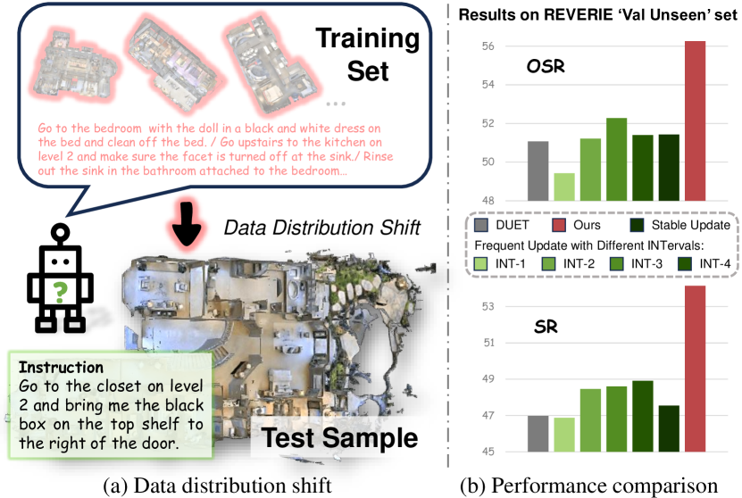
Figure 1: (a) Illustration of the data distribution shift between training and testing samples in the VLN Task. (b) Comparison between various TTA strategies on REVERIE [52] validation unseen set using OSR and SR metrics. Among them, ‘DUET’ [11] is the base model, ‘Frequent Update’ means updating at certain intervals within each sample, ‘Stable Update’ refers to initializing with the original base model for each sample and using its best in-sample update interval INT=1. All these strategies adopt TENT [68] for model updates. The results show that overly fast or overly slow TTA fail to achieve significant improvements.

In the VLN task, agents are required to sequentially execute actions contingent upon the evolving environmental cues. Regrettably, owing to disparities in environmental factors, such as distinct room types and objects as shown in Figure 1(a), the trained agents inevitably confront significant shifts in data distribution when applied in practical scenarios [20, 22]. In light of this issue, depending solely on a pre-trained and fixed VLN model is inadequate.

Recently, Test-Time Adaptation (TTA) [39, 40, 51, 71] has been recognized as an effective technique for leveraging unlabeled test samples to update models and address shifts in data distribution. It has garnered notable success across various computer vision tasks, such as image classification [68, 51], segmentation [71, 67], and video classification [42, 80]. For instance, TENT [68] utilizes an entropy minimization objective to update model parameters, thereby enhancing the generalization ability to recognizing test data. Nonetheless, the application of TTA in the realm of VLN remains relatively uncharted. Although prevailing TTA methodologies can be integrated into VLN models with certain alterations, this direct application cannot well handle the adaptability-stability dilemma of models due to the multi-step action-execution nature of VLN. Specifically, in contrast to traditional classification tasks, where a single TTA operation suffices for a test sample, VLN mandates an agent to perform sequential actions within a single test sample. On one hand, while conducting TTA at every (or a few) action steps enables rapid agent adaptation to dynamic environments, frequent model updates may introduce significant model alterations, potentially causing cumulative errors and catastrophic forgetting [71, 50, 60], thus compromising model stability during testing. On the other hand, initializing the same model for stable TTA in each test sample may hinder the model’s ability to adaptively learn experience from historical test samples, thereby impeding its potential for achieving superior performance.  Figure 1(b) shows that both overly fast or overly slow model updates fail to achieve significant performance improvements.

To tackle the above issues, we proposes a Fast-Slow Test-Time Adaptation (FSTTA) method for the VLN tasks. Built upon a unified gradient-parameter decomposition-accumulation framework, our approach consists of a fast update phase and a slow update phase, pursuing a balance between adaptability and stability in model updates. Specifically, with a test-time training objective, such as entropy minimization, we can derive gradients at each action step in the fast update phase. However, due to the unsupervised nature of TTA, these gradients inevitably contain noise information. Using these gradients for model update can interfere with the adaptability, especially when the update is frequently invoked. Therefore, we attempt to find a reliable optimization direction by periodically analyzing the gradients generated during the recent multi-step navigation process. We first establish a local coordinate system to decompose these gradients into components with varying levels of consistency. Subsequently, these components are adaptively accumulated to pinpoint a concordant direction for updating the model. Besides, a gradient variance regularization is incorporated to dynamically adjust the learning rate.

After a certain number of fast updates, the model parameters (also called model state) are recorded. To further mitigate the issues of cumulative errors and catastrophic forgetting that may result from excessively frequent model updates, during the slow update phase, we revert the model to its historical state and conduct a decomposition-accumulation analysis on the parameter variation trajectory for a direct model update. This process is akin to the fast phase but shifts its focus from gradients to the parameters. Both phases are performed alternately during testing to balance the adaptability and stability of the model. As shown in Figure 1(b), the proposed method achieves significant improvement against other model update strategies.

Our contributions can be summarized as follows:

• We investigate the test-time adaptation within the realm of VLN. Our proposed method verifies TTA as a promising and viable avenue for enhancing VLN performance.

• Based on a unified decomposition-accumulation framework for both gradients and parameters, our method ensures swift model adaptability to environmental changes in the short-term fast update phase, while preserves stability throughout the long-term slow update phase.

• Our FSTTA elevates the performance of several leading VLN models across four popular benchmarks. When applied to the notable DUET model [11], our method yields a performance boost of over $5\%$ on the representative discrete/continuous datasets REVERIE/R2R-CE. Furthermore, our method shows superior results compared to other premier TTA techniques.

2 Related Work

Vision-and-Language Navigation (VLN). Recently, VLN tasks have received significant attention in the embodied AI domain and a variety of effective approaches have been proposed [3, 86, 20]. Most existing methods facilitate VLN research by developing powerful techniques for model training, including: (i) Designing advanced network architectures. Sequence-to-sequence framework are the most commonly used one for predicting agent actions from a historical observation series. Early VLN models utilize LSTMs with various attention mechanisms [3, 16, 46, 24] while recent ones [23, 25, 9, 41, 11, 27, 1] resort to the more popular transformer-based methods for multi-modal pre-training. Other architectures are also explored such as graph neural networks [86] and parameter-efficient adapter [55]. (ii) Adopting various training paradigms such as reinforcement and imitation learning [49, 63, 74, 17]. Moreover, to estimate the completeness of instruction following and decide when to conduct backtracking, progress monitoring [45, 85] and back-tracking [30, 46] are also employed to promote training process. (iii) Performing data augmentation for training a stronger model. In recent years, more and more large-scale benchmarks are established via collecting human annotations [33, 86, 57] or creating new environments [52, 10]. Other approaches explore techniques such as mixup and synthesis [43, 29], style transfer [37], or future-view image semantics [36] for data augmentation. (iv) Leveraging additional information for boosting model capacity. Since the goal of VLN is to navigate in photo-realistic environments, there are many kinds of information in the world that can be used such as knowledge [38], 3D scene geometry [44, 78], and landmarks [72, 12]. Though the above approaches have attempted to employ fruitful strategies for training an effective VLN model, they still struggle to adequately address the domain discrepancy between training and testing data. Some studies [55, 54] have tried to use dynamic networks or auxiliary models to cope with varying test data, however, these approaches neither directly minimize the domain gap between the model and test data nor offer dynamic model update strategies.

Test-time Adaptation (TTA). TTA, which allows models to adapt the test data in an online and unsupervised manner, has gained a lot of interest with a host of various approaches proposed in the literature [39, 40, 61, 73, 34]. Existing TTA methods generally rely on batch normalization calibration [48, 84, 19], entropy minimization [68, 51, 50, 64], auxiliary self-supervised task or data regularization [62, 28, 5, 83, 66] to acquire useful information for reducing the domain gap between training and testing data. To stabilize adaptation in continuously changing data distribution, recently, continual test-time adaptation [71, 50, 60, 6, 13, 82], as a more practical setting, has been tentatively explored for addressing the cumulative errors and catastrophic forgetting issues. Until now, test-time adaptation has been preliminarily explored in some sequential data analysis fields such as action recognition [42] and video classification [80]. However, TTA on VLN tasks is yet to be explored.

Gradient-based Methods. Gradients are typically central to modern SGD-based deep learning algorithms. To date, gradient analysis research has predominantly focused on domain generalization (DG) [47, 35, 70, 56, 76, 65], due to the negative impact of conflicting gradients from multiple domains on model optimization. Pioneering works [15, 81, 47] perform gradient surgery at the backpropagation phase via various strategies such as normal plane projection [81] and consensus learning [47]. Other approaches resort to gradient agreement regularization for refining the optimization direction by leveraging sharpness [70] or similarity [58, 56] measurements. Different from the above models that only consider a single-phase gradient surgery in DG, we jointly analyze the gradient-parameter states for a two-phase (fast-slow) TTA in the VLN task.

3 Our Approach

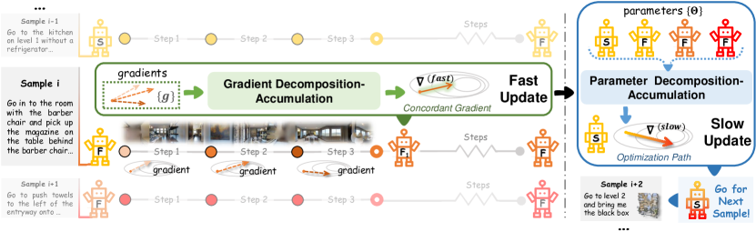
Figure 2: Overall framework of the proposed Fast-Slow Test-Time Adaptation (FSTTA) for VLN tasks. In the fast update phase, taking ‘Sample i’ as an example, the model periodically analyzes the gradients ($\{\bm{g}\}$) generated during the recent multi-step navigation and performs a gradient decomposition-accumulation analysis to pinpoint a concordant direction for model update. After a certain number of fast updates, historical model parameters ($\{\bm{\Theta}\}$) are recorded. In the slow update phase, we revert the model to its historical state and conduct a parameter decomposition-accumulation analysis to learn an optimization path for direct parameter modulation. Note that ‘F’, ‘S’ in the robots means the model parameters after fast and slow updates. ‘$\text{F}_{1}$’ indicates the first fast update within a test sample.

3.1 Preliminaries and Framework Overview

Problem Setup and VLN Base Model. Given a natural language instruction $\bm{I}$, the VLN task requires an agent to find the target viewpoint through the environment by executing a series of actions. During the navigation process, an undirected exploration graph $\mathcal{G}_{t}=(\mathcal{V}_{t},\mathcal{E}_{t})$ is progressively constructed, where $\mathcal{V}_{t}$ denotes navigable nodes, $\mathcal{E}_{t}$ indicates the connectivity edges, $t$ is the current timestep. At this moment, the agent receives a panoramic view that contains 36 single images. The panorama is represented by the image features $\mathcal{R}_{t}$ and their object features $\mathcal{O}_{t}$, where these features can be extracted by pre-trained vision transformers (ViT) [14, 11, 38]. To accomplish the instruction, the agent needs to predict probabilities for the currently navigable nodes and select the most possible one as the next movement action. The probabilities can be predicted as:

$$\bm{s}_{t}=\phi\left(\bm{I},\mathcal{R}_{t},\mathcal{O}_{t},\mathcal{H}_{t};\bm{\Theta}\right),~{}~{}\bm{s}_{t}\in\mathbb{R}^{|\mathcal{V}_{t}|}$$ (1)

where $\mathcal{H}_{t}$ indicates the history information that encodes the observed visual features and performed actions [11, 55]. $\phi(\cdot)$ is the VLN base model such as the dual-scale graph transformer [11, 10], $\bm{\Theta}$ is the learnable model parameters.

Framework Overview. In this paper, we devote to adjusting the VLN base model during testing process within an unsupervised manner. Our FSTTA framework is illustrated in  Figure 2. For each sample, at timestep $t$, we employ the commonly adopted entropy minimization objective [68, 51] for test-time adaption, which aims to reduce the entropy of the probabilities over the current navigable nodes:

$$\mathcal{L}({\bm{s}}_{t};\bm{\Theta})=-\sum\nolimits_{i}{\bm{s}}_{t,i}\log({\bm{s}}_{t,i}).$$ (2)

During the optimization of the above objective, gradients are back-propagated for updating the model’s parameters. However, updating the whole base model is computationally infeasible. As a result, we only consider a small portion of the model parameters for gradient calculation. Since affine parameters in normalization layers capturing data distribution information, numerous TTA methods opt to update these parameters for adaption [68, 51, 39]. In this paper, we employ the model’s final a few layer-norm operations for TTA and maintain other parameters frozen. For brevity, we still use the symbol $\bm{\Theta}$ to represent these parameters to be updated, $\bm{\Theta}\in\mathbb{R}^{D}$. Targeting at fully leveraging the gradient and parameter information, under a unified decomposition-accumulation analysis framework, we propose an effective two-phase adaptation for fast and slow model updates.

3.2 Fast Update via Gradient Analysis

At timestep $t$ in the navigation process, the agent is required to select an action (navigable node) by using the predicted score ${\bm{s}}_{t}$. With this score, we can calculate the TTA loss (Eq. (2)) and then derive the gradient of the model parameters $\bm{\Theta}$ as: $\bm{g}_{t}=\nabla\mathcal{L}({\bm{s}}_{t};\bm{\Theta})$, $\bm{g}_{t}\in\mathbb{R}^{D}$. Traditional TTA methods conduct adaptation independently at each time step, which can exacerbate the issue of cumulative errors [50, 60], particularly in the VLN process that requires frequent action execution. Therefore, we propose to conduct a gradient decomposition-accumulation analysis, wherein we periodically analyze the gradients generated during the recent multi-step navigation process and identify a concordant direction for an iteration of model update.

Gradient Decomposition-Accumulation. During navigation, as shown in Figure 2, we perform model update every $M$ action steps. For the $j$-th update, gradients from previous $M$ steps are collected as $\bm{G}_{j}=\{\widetilde{\bm{g}}_{j,m}\}_{m=1}^{M}$, where $\bm{G}_{j}\in\mathbb{R}^{M\times D}$, $\widetilde{\bm{g}}_{j,m}$ indicates the $t$-th gradient $\bm{g}_{t}$ when $t=M(j-1)+m$. Note that these gradients determines the learning direction of our VLN model, and a simple strategy to compute this direction is to take their average $\bar{\bm{g}}_{j}=1/M\sum_{m}\widetilde{\bm{g}}_{j,m}$; however, this inevitably introduce step-specific noise. To avoid the issue, we aim to find a concordant direction among these gradients. We first establish a local coordinate system with $D$ orthogonal and unit axes (bases) $\bm{U}_{j}=\{{\bm{u}_{j,d}}^{\mathsf{T}}\}_{d=1}^{D}\in\mathbb{R}^{D\times D}$ for gradient decomposition, where each gradient can be approximatively linearly represented by these bases. Intuitively, the axes along which the gradients exhibit the higher variance after projection represent the directions of gradients with the lower consistency. These directions have the potential to introduce interference in determining a model update direction. Therefore, it is advisable to reduce the projection of gradients in these directions. To solve the bases $\bm{U}_{j}$, we can utilize singular value decomposition (SVD) as follows:

$$\lambda_{j,d},\bm{u}_{j,d}=\textbf{SVD}_{d}\left(\frac{1}{M-1}{\hat{\bm{G}}}_{j}^{\mathsf{T}}\hat{\bm{G}}_{j}\right),$$ (3)

where $\hat{\bm{G}}_{j}$ is the centered gradient matrix by removing the mean from $\bm{G}_{j}$. The $m$-th row vector in $\hat{\bm{G}}_{j}$ reflects the deviation between $\widetilde{\bm{g}}_{j,m}$ and the average gradient $\bar{\bm{g}}_{j}$. $\lambda_{j,d}$, $\bm{u}_{j,d}$ denote the $d$-th largest eigenvalue and the corresponding eigenvector. Motivated by the principle component analysis [59], it is obvious that a larger $\lambda_{j,d}$ corresponds to a higher variance of the gradient projection length $\bm{G}_{j}\bm{u}_{j,d}$ and vice versa. Hence, we can derive a concordant gradient by adaptively aggregating the gradients’ components on all the axes by considering different eigenvalue (importance):

$$\nabla_{j}^{(fast)}=\sum\nolimits_{d=1}^{D}\Phi_{d}(\lambda_{j,d})\cdot<\bar{\bm{g}}_{j},\bm{u}_{j,d}>\bm{u}_{j,d},$$ (4)

where the last term denotes the projected component of the averaged gradient $\bar{\bm{g}}_{j}$ on to the $d$-th axis. $\Phi_{d}(\cdot)$ is referred as the adaptive coefficient for accumulating all the components, which is simply defined as $\Phi_{d}(\lambda_{j,d})=1/\lambda_{j,d}$, reflecting the importance of various axes. Notably, when removing the coefficient, $\nabla_{j}^{(fast)}$ is degenerated into $\bar{\bm{g}}_{j}$, which is used in regular gradient descent approaches.

Based on Eq. (4), a concordant optimization direction is established by enhancing the components that are convergent among $\{\widetilde{\bm{g}}_{j,m}\}_{m=1}^{M}$ and suppressing those divergent ones. However, the introduction of $\Phi_{d}(\cdot)$ makes the length of $\nabla_{j}^{(fast)}$ uncontrollable. Therefore, we calibrate its length to $\left\|\bar{\bm{g}}_{j}\right\|_{2}$, which encodes the gradient length from the last three time steps, for a more reasonable model update:

$$\nabla_{j}^{(fast)}\leftarrow(\nabla_{j}^{(fast)}\|\bar{\bm{g}}_{j}\|_{2})/\|\nabla_{j}^{(fast)}\|_{2}$$ (5)

With $\nabla^{(fast)}$, we can perform fast model update by setting a learning rate $\gamma^{(fast)}$. Although traditional methods employ a fixed learning rate during optimization, such a setting might hinder model convergence, i.e., small learning rates slow down convergence while aggressive learning rates prohibit convergence [4]. Since fast updates are frequently invoked during navigation, relying on a fixed learning rate is sub-optimal. Therefore, we propose to dynamically adjust learning rate throughout the fast update phase.

Dynamic Learning Rate Scaling. Different from varying the learning rate through optimizer or scheduler, we argue for a scaling method that leverages gradient agreement information in historical steps to dynamically adjust the speed of model update. Current gradient alignment strategies typically impose direct constraints on the gradients [58, 56], which are not suitable for our framework as they undermine the gradient decomposition-accumulation process. Given that the second-order information (variance) has been demonstrated to be more effective than the first-order information (mean) in gradient agreement learning [56], we directly utilize the trace of the gradient covariance matrix, $\text{Tr}\left(1/(M-1){\hat{\bm{G}}}_{j}^{\mathsf{T}}\hat{\bm{G}}_{j}\right)$, for scaling. Note that the trace is equal to the sum of eigenvalues $\sigma_{j}=\sum_{d}\lambda_{j,d}$. Here, when $\sigma_{j}$ deviates significantly from the historical variance, we assign a smaller learning rate, and vice versa:

$$\gamma^{(fast)}_{j}=\text{Trunc}\left(1+\tau-|\sigma_{j}-\bar{\sigma}|\right)\cdot\hat{\gamma}^{(fast)},$$ (6)

where $\text{Trunc}(\cdot)$ is the truncation function that truncates the input to the interval $[a,b]$. $\tau$ is a threshold and $\hat{\gamma}^{(fast)}$ is the base learning rate. The historical variance $\bar{\sigma}$ is updated as $\bar{\sigma}\leftarrow\rho\bar{\sigma}+(1-\rho)\sigma_{j}$ and maintained for all samples throughout the test stage, $\rho$ is the update momentum.

Model Update. With the above gradient and learning rate, we can perform the $j$-th fast model update:

$$\bm{\Theta}_{j}=\bm{\Theta}_{j-1}-\gamma_{j}^{(fast)}\cdot\nabla_{j}^{(fast)},$$ (7)

where the subscript of $\bm{\Theta}$ indicates the index of model update in the current test sample.

3.3 Slow Update via Parameter Analysis

In the fast update phase, although we obtain concordant optimization directions, the frequent parameter updates may still dramatically change the VLN model. To maintain the stability of the VLN model during long-term usage, we revert the model to its historical states recorded in the fast update phase, and conduct a decomposition-accumulation analysis on the parameter variation trajectory for direct parameter modulation. The slow update phase shares the core formulation with the fast phase, but shifts the focus from gradients to the model parameters themselves.

Parameter Decomposition-Accumulation. Following the completion of the fast update phase on the $o$-th test sample, the model state (parameters) is recorded as $\bm{\Theta}_{o,J_{o}}$, where $J_{o}$ denotes the final fast update step on this sample, and the subscript $o$ has been omitted in the previous section. We then treat these historical states as a parameter variation trajectory to facilitate stable model updates. As shown in the right part of Figure 2, the slow model update is invoked every $N$ samples. For the $l$-th update, historical model states are collected as $\bm{M}_{l}=\{\widetilde{\bm{\Theta}}_{l,n}\}_{n=0}^{N}$, where $\bm{M}_{l}\in\mathbb{R}^{(N+1)\times D}$, $\widetilde{\bm{\Theta}}_{l,n}$ indicates the $o$-th model state $\bm{\Theta}_{o,J_{o}}$ when $o=N(l-1)+n$ and $n\neq 0$. $\widetilde{\bm{\Theta}}_{l,0}$ indicates the model state produced by the previous slow update, and we use it interchangeably with $\bm{\Theta}^{(l-1)}$ in the following. Note that in the slow update phase, we additionally incorporate $\bm{\Theta}^{(l-1)}$ from the previous update for analysis since it serves as a starting reference point for direct parameter modulation.

Table 1: Comparison on REVERIE. Results better than the base model are highlighted in bold.

Methods	REVERIE Val Unseen						REVERIE Test Unseen
	TL $\downarrow$	OSR	SR	SPL	RGS	RGSPL	TL $\downarrow$	OSR	SR	SPL	RGS	RGSPL
Human	-	-	-	-	-	-	21.18	86.83	81.51	53.66	77.84	51.44
Seq2Seq [3] [CVPR18]	11.07	8.07	4.20	2.84	2.16	1.63	10.89	6.88	3.99	3.09	2.00	1.58
RCM [74] [CVPR19]	11.98	14.23	9.29	6.97	4.89	3.89	10.60	11.68	7.84	6.67	3.67	3.14
SMNA [45] [ICLR19]	9.07	11.28	8.15	6.44	4.54	3.61	9.23	8.39	5.80	4.53	3.10	2.39
FAST [52] [CVPR20]	45.28	28.20	14.40	7.19	7.84	4.67	39.05	30.63	19.88	11.61	11.28	6.08
Airbert [21] [ICCV21]	18.71	34.51	27.89	21.88	18.23	14.18	17.91	34.20	30.28	23.61	16.83	13.28
HAMT [9] [NeurIPS21]	14.08	36.84	32.95	30.20	18.92	17.28	13.62	33.41	30.40	26.67	14.88	13.08
HOP [53] [CVPR22]	16.46	36.24	31.78	26.11	18.85	15.73	16.38	33.06	30.17	24.34	17.69	14.34
LANA [75] [CVPR23]	23.18	52.97	48.31	33.86	32.86	22.77	18.83	57.20	51.72	36.45	32.95	22.85
BEVBert [1] [ICCV23]	-	56.40	51.78	36.37	34.71	24.44	-	57.26	52.81	36.41	32.06	22.09
BSG [44] [ICCV23]	24.71	58.05	52.12	35.59	35.36	24.24	22.90	62.83	56.45	38.70	33.15	22.34
GridMM [78] [ICCV23]	23.20	57.48	51.37	36.47	34.57	24.56	19.97	59.55	55.13	36.60	34.87	23.45
DUET [11] [CVPR22]	22.11	51.07	46.98	33.73	32.15	23.03	21.30	56.91	52.51	36.06	31.88	22.06
DUET-FSTTA	22.14	56.26	54.15	36.41	34.27	23.56	21.52	58.44	53.40	36.43	32.99	22.40
HM3D [10] [ECCV22]	22.13	62.11	55.89	40.85	36.58	26.76	20.87	59.81	53.13	38.24	32.69	22.68
HM3D-FSTTA	22.37	63.74	57.02	41.41	36.97	26.55	21.90	63.68	56.44	39.58	34.05	23.04

Table 2: Results on R2R dataset.

Methods	R2R Val Unseen
	TL $\downarrow$	NE $\downarrow$	SR	SPL
Seq2Seq [3]	8.39	7.81	22	-
RCM [74]	11.46	6.09	43	-
SMNA [45]	-	5.52	45	32
EnvDrop [63]	10.70	5.22	52	48
AirBert [21]	11.78	4.10	62	56
HAMT [9]	11.46	3.65	66	61
GBE [86]	-	5.20	54	43
SEvol [7]	12.26	3.99	62	57
HOP [53]	12.27	3.80	64	57
BEVBert [1]	14.55	2.81	75	64
LANA [75]	12.00	-	68	62
BSG [44]	14.90	2.89	74	62
GridMM [78]	13.27	2.83	75	64
DUET [11]	13.94	3.31	72	60
DUET-FSTTA	14.64	3.03	75	62
HM3D [10]	14.29	2.83	74	62
HM3D-FSTTA	14.86	2.71	75	63

Similar to the fast update phase, the centered parameter matrix $\hat{\bm{M}}_{l}$ can be constructed, where the $n$-th row vector in it reflects the deviation between $\widetilde{\bm{\Theta}}_{l,n}$ and the averaged historical parameter $\bar{\bm{\Theta}}_{l}=1/(N+1)\sum_{n}\widetilde{\bm{\Theta}}_{l,n}$. With $\hat{\bm{M}}_{l}$, we can obtain the following eigenvalues and eigenvectors: $\epsilon_{l,d},\bm{z}_{l,d}=\textbf{SVD}_{d}(1/N\cdot{\hat{\bm{M}}}_{l}^{\mathsf{T}}\hat{\bm{M}}_{l})$, where a larger $\epsilon_{l,d}$ corresponds to a higher variance of the parameter projection length ${\bm{M}}_{l}\bm{z}_{l,d}$ and vice versa. $\bm{Z}_{l}=\{{\bm{z}_{l,d}}^{\mathsf{T}}\}_{d=1}^{D}$ depicts the local coordinate system where each axis depicts the direction of parameter variation. Intuitively, the principal axes (with larger eigenvalues) delineate the primary directions of historical parameter variation, while minor axes (with smaller eigenvalues) often encompass noise [76]. To find a more reliable optimization path to traverse the trajectory of primary parameter changes, we pay more attention on the axis with the larger variance. Since there is no silver bullet to learning an optimization direction with only parameters, a reference direction can significantly aid in guiding the model towards a local optimal. Here, we leverage the parameter variations to calculate the reference direction:

$$\bm{h}_{l}=\frac{1}{\sum_{i=0}^{N-1}q^{i}}\sum\nolimits_{n=1}^{N}q^{N-n}\cdot(\widetilde{\bm{\Theta}}_{l,0}-\widetilde{\bm{\Theta}}_{l,n}),$$ (8)

where the hyper-parameter $q\in(0,1)$, which assigns larger weight to the more recent parameter deviations as they encapsulate richer sample information. Then, we calculate the optimization path (gradient) in the slow update phase as:

$$\nabla_{l}^{(slow)}=\sum\nolimits_{d}\Psi_{d}(\bm{\epsilon}_{l},\bm{h}_{l})\cdot\text{sign}\left(<\bm{h}_{l},\bm{z}_{l,d}>\right)\bm{z}_{l,d},$$ (9)

where the use of sign function $\text{sign}(\cdot)$ is to force the axes to be positively related to the reference direction $\bm{h}_{l}$. Notably, different from Eq. (4) that uses the projected components on each axis for estimating an optimization direction, here we only utilize the axes themselves for deriving $\nabla_{l}^{(slow)}$. The reason is that these axes depict the parameter variation direction, which can be directly used for estimating gradients. $\Psi_{d}(\cdot)$ is referred as the adaptive coefficient for accumulating all the axes (optimization directions), defined as:

$$\Psi_{d}(\bm{\epsilon}_{l},\bm{h}_{l})=\frac{\epsilon_{l,d}\cdot\|\bm{h}_{l}\|_{2}}{\|\bm{\epsilon}_{l}\|_{2}},$$ (10)

where the L2-normalization is performed on eigenvalues to convey different relative importance of axes. Besides, the norm of the reference direction is utilized to automatically tuning the magnitude of the analyzed gradient. In contrast to $\Phi_{d}(\cdot)$ in gradient analysis, $\Psi_{d}(\cdot)$ highlights those axes with high variation due to the different characteristics of gradients and parameters in model optimization.

Model Update. With $\nabla_{l}^{(slow)}$, we can perform the $l$-th slow model update as follows:

$$\bm{\Theta}^{(l)}=\bm{\Theta}^{(l-1)}-\gamma^{(slow)}\cdot\nabla_{l}^{(slow)},$$ (11)

where $\gamma^{(slow)}$ is learning rate. Since the slow update phase is designed for stable model learning and is not frequently invoked, we employ a fixed learning rate here instead of conducting dynamic learning rate scaling, as done in the fast phase. The updated parameter $\bm{\Theta}^{(l)}$ will be utilized for the subsequent test samples in conjunction with new fast update phases applied to them.

4 Experimental Results

We evaluate FSTTA on four benchmarks: REVERIE [52], R2R [3], SOON [86], and R2R-CE [32] datasets. Experiments and ablation studies show our effectiveness.

4.1 Experimental Setup

Datasets. Four datasets are adopted for conducting our experiments. Among them, REVERIE [52] contains 10,567 panoramic images and 21,702 high-level instructions, focusing on grounding remote target object within 90 buildings. R2R [3] provides step-by-step instructions for navigation in photo-realistic environments, which includes 10,800 panoramic views and 7,189 trajectories. SOON [86] also requires the agent to find the target object with a more detailed description of the goal. It has 3,848 sets of instruction and more than 30K long distance trajectories. R2R-CE [32] is a variant of R2R in continuous environments, where an agent is able to move freely and engage with obstacles. The dataset consists of 16,000 instruction-trajectory pairs, with non-transferrable paths excluded.

Evaluation Metrics. We follow previous approaches [52, 11, 10, 37, 78] and employ the most commonly used metrics for evaluating VLN agents as follows: TL (Trajectory Length), NE (Navigation Error), SR (Success Rate), SPL (Success weighted by Path Length), OSR (Oracle Success Rate), RGS (Remote Grounding Success rate), and RGSPL (RGS weighted by Path Length).

Implementation Details. To better conform to practical scenarios, for all datasets, we set the batch size to 1 during evaluation. Each sample (or each action step) is forward propagated only once during the testing process. We adopt DUET [11] and HM3D [10] as the base models. Since HM3D does not provide training code for R2R-CE dataset, we adopt another state-of-the-art method, BEVBert [1], for TTA. Note that for the base models, in Section 4.2, we report the results obtained from running their official codes. For VLN models equipped with TTA strategies, we run the corresponding experiments 5 times while shuffling the order of the samples and report the average results. In our FSTTA, we only utilize the last four LN layers of base models for model updating, all the feature dimensions of these layers are 768. We set the intervals for fast and slow updates to $M=3$ and $N=4$, the learning rates of the two phases are $\hat{\gamma}^{(fast)}=6\times 10^{-4}$ and $\gamma^{(slow)}=1\times 10^{-3}$. For the dynamic learning rate scaling, we empirically set the threshold $\tau=0.7$ in Eq. (6) and the update momentum $\rho=0.95$ with the truncation interval $[0.9,1.1]$. And the hyper-parameter $q$ in Eq. (8) is set to 0.1. All experiments are conducted on a RTX 3090 GPU.

4.2 Comparison with State-of-the-art VLN Models

REVERIE. Table 2 presents a comparison of our FSTTA against state-of-the-art methods on the REVERIE dataset. Compared with the base models which do not perform test-time adaptation, the proposed method demonstrates favorable performance improvement across most evaluation metrics across the two dataset splits. Specifically, on the validation unseen split, our model exhibits notable advantages over DUET, with improvements of 5.3% on OSR, 7.1% on SR, and 2.7% on SPL. Furthermore, for the recent state-of-the-art method HM3D, our model displays enhanced generalization capabilities on the test unseen split, achieving remarkable improvements over HM3D, including 3.9%, 3.3%, and 1.3% increases on the three metrics. Compared with other state-of-the-arts, our proposed method can achieve superior or comparable performance. These results unequivocally affirm the effectiveness of our fast-slow test time adaptation model, showing the promising potential of TTA in the VLN field. It is noteworthy that none of the prior methods employed a TTA strategy on this task.

R2R. Table 2 shows the comparison results on R2R dataset. Our approach outperforms the base models in most metrics (e.g., $72\%\rightarrow 75\%$ for DUET on SR, $62\%\rightarrow 63\%$ for HM3D on SPL). Notably, from the results of the above two datasets, our method, while enhancing the success rate of VLN, causes a slight increase in the path length (TL). We speculate that a possible reason is that performing TTA online may increase the likelihood of the agent deviating from its original action execution pattern, leading to more exploration or backtracking. This situation is further confirmed in the analysis of various TTA strategies in Table 5.

SOON. The proposed FSTTA establishes new state-of-the-art results across most metrics on this dataset. For instance, as shown in Table 3, on the validation unseen split, our model HM3D-FSTTA achieves SR and SPL of 42.44% and 31.03%, respectively, while the state-of-the-art method GridMM are 37.46% and 24.81%. On the test unseen split, our approach improves the performance of DUET by substantial gains (e.g., $21.42\%\rightarrow 23.23\%$ for SPL).

Table 3: Experimental results on SOON dataset.

Methods	Val Unseen				Test Unseen
	OSR	SR	SPL	RGSPL	OSR	SR	SPL	RGSPL
GBE [86]	28.54	19.52	13.34	1.16	21.45	12.90	9.23	0.45
GridMM [78]	53.39	37.46	24.81	3.91	48.02	36.27	21.25	4.15
DUET [11]	50.91	36.28	22.58	3.75	43.00	33.44	21.42	4.17
DUET-FSTTA	52.57	36.53	23.82	3.75	43.44	35.34	23.23	4.52
HM3D [10]	53.22	41.00	30.69	4.06	47.26	40.26	28.09	5.15
HM3D-FSTTA	54.19	42.44	31.03	4.93	48.52	42.02	28.95	5.20

R2R-CE. FSTTA also generalizes well on the continuous environment, i.e., R2R-CE dataset, as shown in Table 4. The results indicate that our approach demonstrates superior or comparable performance against other methods across several metrics.

Table 4: Experimental results on R2R-CE dataset.

Methods	Val Unseen				Test Unseen
	NE $\downarrow$	OSR	SR	SPL	NE $\downarrow$	OSR	SR	SPL
Seq2Seq [32]	7.37	40	32	30	7.91	36	28	25
CWTP [8]	7.90	38	26	23	-	-	-	-
CM2 [18]	7.02	42	34	28	7.70	39	31	24
Sim2Sim [31]	6.07	52	43	36	6.17	52	44	37
CWP-BERT [26]	5.74	53	44	39	5.89	51	42	36
DREAMW [69]	5.53	49	59	44	5.48	49	57	44
GridMM [78]	5.11	61	49	41	5.64	56	46	39
ETPNav [2]	4.71	65	57	49	5.12	63	55	48
DUET [11]	5.13	55	46	40	5.82	50	42	36
DUET-FSTTA	5.27	58	48	42	5.84	55	46	38
BEVBert [1]	4.57	67	59	50	4.70	67	59	50
BEVBert-FSTTA	4.39	65	60	51	5.45	69	60	50

Table 5: Experimental results for different TTA strategies.

Methods	REVERIE Val Unseen						Time(ms)
	TL $\downarrow$	OSR	SR	SPL	RGS	RGSPL
DUET [11]	22.11	51.07	46.98	33.73	32.15	23.03	104.84
+ EATA [50]	23.41	52.09	47.40	33.46	32.09	22.65	133.12
+ CoTTA [71]	24.88	52.46	47.56	31.43	31.82	21.83	3.89$\times$ 103
+ NOTE [19]	23.15	52.85	48.28	33.98	32.77	22.98	137.89
+ SAR [51]	23.47	53.26	48.00	33.92	33.49	23.09	145.53
+ Tent [68]	24.05	49.43	46.87	31.90	30.04	20.15	126.91
+ Tent-INT-2	24.24	51.22	48.46	33.67	32.43	21.30	124.02
+ Tent-INT-3	22.52	52.28	48.60	34.65	32.66	23.12	119.34
+ Tent-INT-4	22.59	51.40	48.91	35.06	32.59	22.99	117.26
+ Tent-Stable	22.05	51.43	47.55	33.99	32.34	23.32	129.22
+ FSTTA	22.14	56.26	54.15	36.41	34.27	23.56	135.61

4.3 Results for Different TTA Strategies

Currently, various TTA methods have been adeptly integrated for the dynamic model updates within diverse computer vision tasks, marking significant progress. Although the exploration of TTA’s application within the VLN field remains relatively untapped, the integration of contemporary advanced TTA methodologies into VLN is feasible. Since efficiency is an important evaluation metric for TTA, we provide the average time taken by each method to execute a single instruction for comparison. Obviously, equipping with TTA inevitably incurs additional time costs. For the compared methods, SAR and TENT are the popular entropy minimization models, whereas NOTE, CoTTA, and EATA are state-of-the-art continual TTA methods. The results in Table 5 demonstrate the capability of our proposed FSTTA to blend model performance with testing efficiency. Specifically, on the validation unseen dataset of REVERIE, our method exhibits a discernible enhancement of 6.2% and 2.5% on the SR and SPL metrics compared to the state-of-the-art SAR method, concurrently manifesting a reduction of 7% in testing time. From the results, directly applying existing TTA methods to the VLN task does not lead to significant performance improvements. Furthermore, we investigate different frequencies of updates based on TENT as well as the stable update approach. ‘INT’ represents the update interval, which means averaging the gradient information over a certain interval and then performing an iteration of model update; these results are consistent with those in Figure 1(b). It can be seen that our method still outperforms these strategies with marginally increased time costs.

Table 6: Ablation study on REVERIE dataset.

Module			REVERIE Val Unseen
Fast	DLR	Slow	TL $\downarrow$	OSR	SR	SPL	RGS	RGSPL
-	-	-	22.11	51.07	46.98	33.73	32.15	23.03
Tent	-	-	22.52	52.28	48.60	34.65	32.66	23.12
✓	-	-	22.65	53.50	49.74	34.91	33.70	23.36
✓	✓	-	22.43	54.01	49.82	35.34	34.32	23.29
✓	✓	✓	22.14	56.26	54.15	36.41	34.27	23.56

Table 7: Results on validation seen set of REVERIE.

FSTTA		REVERIE Val Seen
Unseen	Seen	TL $\downarrow$	OSR	SR	SPL	RGS	RGSPL
-	-	13.86	73.86	71.15	63.94	57.41	51.14
-	✓	15.13	75.59	75.48	65.84	58.62	52.23
✓	-	13.40	73.16	71.78	64.18	57.05	51.18
✓	✓	15.11	75.58	74.12	65.53	59.20	52.18

4.4 Further Remarks

We perform ablation studies and other in-depth analysis of FSTTA on the validation unseen set of REVERIE [52].

Ablation Studies of the Proposed FSTTA. In this work, we propose a FSTTA method for vision-and-language navigation, which consists of both fast and slow model update phases. To validate their effectiveness, we progressively integrate the two phases into the baseline DUET model. In addition, we design a baseline variant, which equips DUET with the vanilla TTA objective (TENT [68]) and simply utilize the averaged gradient in an interval (with the same $M$) for fast model updates. Empirical findings from Table 6 illuminate that the integration of fast and slow phases progressively bolsters the base model by 2.8% and 4.3% on the SR metric. Moreover, the dynamic learning rate scaling module (DLR) also contributes to enhancing the model’s performance. Furthermore, our method surpasses the vallina TTA method by a significant margin, showing the consideration of the fast-slow update mechanism is effective.

Will our method experience catastrophic forgetting? For a VLN agent endowed with the TTA capability, it faces the issue of catastrophic forgetting of historical environments and instructions upon continually executing new instructions in new environments. To assess whether our method harbors this issue, we re-evaluate our methods on REVERIE validation seen data. Compared with the base model, as shown in Table 7, we find that: (1) Directly applying FSTTA with the base model on seen data can noticeably enhance performance. (2) After performing FSTTA on the unseen set, the obtained model, when tested directly on the seen dataset without TTA, achieves performance comparable to the base model, confirming that our method does not suffer from catastrophic forgetting. (3) Applying the updated model from unseen set to the seen set with TTA yields the best results. This indicates that our method is effective in accumulating experience from historical test data.

Generalization Testing in More Practical Environments. In the real-world applications, agents might encounter both previously seen and unseen scenarios. In our preceding experiments, we exclusively test on the validation seen and unseen sets separately. To verify the generalizability, we combine the seen and unseen sets into a unified set. Table 8 shows that FSTTA outperforms other TTA methods in effectively managing a variety of testing scenarios.

Qualitative Analysis. Figure 3 provides a visualization of the agent’s instruction execution process, validating that our proposed FSTTA approach can indeed dynamically enhance the VLN performance of the agent during testing.

Table 8: Results of validation unseen & seen on REVERIE dataset.

Methods	REVERIE Val Unseen & Seen
	TL $\downarrow$	OSR	SR	SPL	RGS	RGSPL
DUET [11]	19.18	61.53	57.49	45.66	41.56	34.38
+ Tent [68]	20.23	57.33	54.86	41.90	38.09	32.46
+ EATA [50]	20.29	62.77	57.31	44.59	41.54	34.16
+ SAR [51]	20.52	63.59	57.80	44.72	42.45	34.88
+ FSTTA	20.48	63.36	60.23	47.96	43.58	35.65

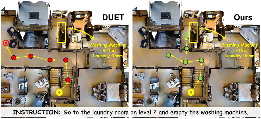
Figure 3: Visual results of DUET [11] and FSTTA on REVERIE validation unseen set. Our method arrives the correct endpoint.

5 Conclusions

This paper explores the feasibility of TTA strategies in VLN. We propose a fast-slow test-time adaptation method, which performs decomposition-accumulation analysis for both gradients and parameters, achieving a balance between adaptability and stability. The encouraging performance is validated in extensive experiments. Several limitations of this paper are noteworthy. Firstly, our approach focuses on adapting normalization layers within the trained model. While normalization layers are widely employed in deep learning, there are still a few methods that do not utilize these settings. One viable approach to address this issue is to introduce additional normalization layers to the corresponding models and retrain them using the training data. In the future, we will also explore how our model can update other types of layers. Secondly, the VLN task itself is a cross-modal learning task. However, our TTA process does not explicitly consider this information. We plan to consider cross-modal TTA in the future. Thirdly, compared to the base model, the introduction of TTA inevitably incurs additional computational cost, which is a direction for future improvement. Finally, the frequencies of fast and slow updates are fixed and periodic. Adaptive update invocation strategies is worthy of consideration.

References

- An et al. [2023a] Dong An, Yuankai Qi, Yangguang Li, Yan Huang, Liang Wang, Tieniu Tan, and Jing Shao. Bevbert: Topo-metric map pre-training for language-guided navigation. In ICCV, 2023a.
- An et al. [2023b] Dongyan An, H. Wang, Wenguan Wang, Zun Wang, Yan Huang, Keji He, and Liang Wang. Etpnav: Evolving topological planning for vision-language navigation in continuous environments. ArXiv, abs/2304.03047, 2023b.
- Anderson et al. [2018] Peter Anderson, Qi Wu, Damien Teney, Jake Bruce, Mark Johnson, Niko Sünderhauf, Ian Reid, Stephen Gould, and Anton Van Den Hengel. Vision-and-language navigation: Interpreting visually-grounded navigation instructions in real environments. In CVPR, 2018.
- Barzilai and Borwein [1988] Jonathan Barzilai and Jonathan Michael Borwein. Two-point step size gradient methods. Ima Journal of Numerical Analysis, 8:141–148, 1988.
- Boudiaf et al. [2022] Malik Boudiaf, Romain Mueller, Ismail Ben Ayed, and Luca Bertinetto. Parameter-free online test-time adaptation. In CVPR, 2022.
- Brahma and Rai [2023] Dhanajit Brahma and Piyush Rai. A probabilistic framework for lifelong test-time adaptation. In CVPR, 2023.
- Chen et al. [2022a] Jinyu Chen, Chen Gao, Erli Meng, Qiong Zhang, and Si Liu. Reinforced structured state-evolution for vision-language navigation. In CVPR, 2022a.
- Chen et al. [2020] Kevin Chen, Junshen Chen, Jo Chuang, Marynel V’azquez, and Silvio Savarese. Topological planning with transformers for vision-and-language navigation. In CVPR, 2020.
- Chen et al. [2021] Shizhe Chen, Pierre-Louis Guhur, Cordelia Schmid, and Ivan Laptev. History aware multimodal transformer for vision-and-language navigation. In NeurIPS, 2021.
- Chen et al. [2022b] Shizhe Chen, Pierre-Louis Guhur, Makarand Tapaswi, Cordelia Schmid, and Ivan Laptev. Learning from unlabeled 3d environments for vision-and-language navigation. In ECCV, 2022b.
- Chen et al. [2022c] Shizhe Chen, Pierre-Louis Guhur, Makarand Tapaswi, Cordelia Schmid, and Ivan Laptev. Think global, act local: Dual-scale graph transformer for vision-and-language navigation. In CVPR, 2022c.
- Cui et al. [2023] Yibo Cui, Liang Xie, Yakun Zhang, Meishan Zhang, Ye Yan, and Erwei Yin. Grounded entity-landmark adaptive pre-training for vision-and-language navigation. In ICCV, 2023.
- Döbler et al. [2023] Mario Döbler, Robert A Marsden, and Bin Yang. Robust mean teacher for continual and gradual test-time adaptation. In CVPR, 2023.
- Dosovitskiy et al. [2020] Alexey Dosovitskiy, Lucas Beyer, Alexander Kolesnikov, Dirk Weissenborn, Xiaohua Zhai, Thomas Unterthiner, Mostafa Dehghani, Matthias Minderer, Georg Heigold, Sylvain Gelly, et al. An image is worth 16x16 words: Transformers for image recognition at scale. In ICLR, 2020.
- Du et al. [2018] Yunshu Du, Wojciech M Czarnecki, Siddhant M Jayakumar, Mehrdad Farajtabar, Razvan Pascanu, and Balaji Lakshminarayanan. Adapting auxiliary losses using gradient similarity. arXiv preprint arXiv:1812.02224, 2018.
- Fried et al. [2018] Daniel Fried, Ronghang Hu, Volkan Cirik, Anna Rohrbach, Jacob Andreas, Louis-Philippe Morency, Taylor Berg-Kirkpatrick, Kate Saenko, Dan Klein, and Trevor Darrell. Speaker-follower models for vision-and-language navigation. In NeurIPS, 2018.
- Gao et al. [2023] Chen Gao, Xingyu Peng, Mi Yan, He Wang, Lirong Yang, Haibing Ren, Hongsheng Li, and Si Liu. Adaptive zone-aware hierarchical planner for vision-language navigation. In CVPR, 2023.
- Georgakis et al. [2022] Georgios Georgakis, Karl Schmeckpeper, Karan Wanchoo, Soham Dan, Eleni Miltsakaki, Dan Roth, and Kostas Daniilidis. Cross-modal map learning for vision and language navigation. In CVPR, 2022.
- Gong et al. [2022] Taesik Gong, Jongheon Jeong, Taewon Kim, Yewon Kim, Jinwoo Shin, and Sung-Ju Lee. Note: Robust continual test-time adaptation against temporal correlation. In NeurIPS, 2022.
- Gu et al. [2022] Jing Gu, Eliana Stefani, Qi Wu, Jesse Thomason, and Xin Wang. Vision-and-language navigation: A survey of tasks, methods, and future directions. In ACL, 2022.
- Guhur et al. [2021a] Pierre-Louis Guhur, Makarand Tapaswi, Shizhe Chen, Ivan Laptev, and Cordelia Schmid. Airbert: In-domain pretraining for vision-and-language navigation. In ICCV, 2021a.
- Guhur et al. [2021b] Pierre-Louis Guhur, Makarand Tapaswi, Shizhe Chen, Ivan Laptev, and Cordelia Schmid. Airbert: In-domain pretraining for vision-and-language navigation. In ICCV, 2021b.
- Hao et al. [2020] Weituo Hao, Chunyuan Li, Xiujun Li, Lawrence Carin, and Jianfeng Gao. Towards learning a generic agent for vision-and-language navigation via pre-training. In CVPR, 2020.
- Hong et al. [2020] Yicong Hong, Cristian Rodriguez-Opazo, Yuankai Qi, Qi Wu, and Stephen Gould. Language and visual entity relationship graph for agent navigation. In NeurIPS, 2020.
- Hong et al. [2021] Yicong Hong, Qi Wu, Yuankai Qi, Cristian Rodriguez-Opazo, and Stephen Gould. Vln bert: A recurrent vision-and-language bert for navigation. In CVPR, 2021.
- Hong et al. [2022] Yicong Hong, Zun Wang, Qi Wu, and Stephen Gould. Bridging the gap between learning in discrete and continuous environments for vision-and-language navigation. In CVPR, 2022.
- Huo et al. [2023] Jingyang Huo, Qiang Sun, Boyan Jiang, Haitao Lin, and Yanwei Fu. Geovln: Learning geometry-enhanced visual representation with slot attention for vision-and-language navigation. In CVPR, 2023.
- Iwasawa and Matsuo [2021] Yusuke Iwasawa and Yutaka Matsuo. Test-time classifier adjustment module for model-agnostic domain generalization. In NeurIPS, 2021.
- Kamath et al. [2023] Aishwarya Kamath, Peter Anderson, Su Wang, Jing Yu Koh, Alexander Ku, Austin Waters, Yinfei Yang, Jason Baldridge, and Zarana Parekh. A new path: Scaling vision-and-language navigation with synthetic instructions and imitation learning. In CVPR, 2023.
- Ke et al. [2019] Liyiming Ke, Xiujun Li, Yonatan Bisk, Ari Holtzman, Zhe Gan, Jingjing Liu, Jianfeng Gao, Yejin Choi, and Siddhartha Srinivasa. Tactical rewind: Self-correction via backtracking in vision-and-language navigation. In CVPR, 2019.
- Krantz and Lee [2022] Jacob Krantz and Stefan Lee. Sim-2-sim transfer for vision-and-language navigation in continuous environments. In ECCV, 2022.
- Krantz et al. [2020] Jacob Krantz, Erik Wijmans, Arjun Majumdar, Dhruv Batra, and Stefan Lee. Beyond the nav-graph: Vision-and-language navigation in continuous environments. In ECCV, 2020.
- Ku et al. [2020] Alexander Ku, Peter Anderson, Roma Patel, Eugene Ie, and Jason Baldridge. Room-across-room: Multilingual vision-and-language navigation with dense spatiotemporal grounding. In EMNLP, 2020.
- Lee et al. [2023] Jungsoo Lee, Debasmit Das, Jaegul Choo, and Sungha Choi. Towards open-set test-time adaptation utilizing the wisdom of crowds in entropy minimization. In ICCV, 2023.
- Lew et al. [2023] Byounggyu Lew, Donghyun Son, and Buru Chang. Gradient estimation for unseen domain risk minimization with pre-trained models. In ICCV, 2023.
- Li and Bansal [2023] Jialu Li and Mohit Bansal. Improving vision-and-language navigation by generating future-view image semantics. In CVPR, 2023.
- Li et al. [2022] Jialu Li, Hao Tan, and Mohit Bansal. Envedit: Environment editing for vision-and-language navigation. In CVPR, 2022.
- Li et al. [2023] Xiangyang Li, Zihan Wang, Jiahao Yang, Yaowei Wang, and Shuqiang Jiang. Kerm: Knowledge enhanced reasoning for vision-and-language navigation. In CVPR, 2023.
- Liang et al. [2023] Jian Liang, Ran He, and Tieniu Tan. A comprehensive survey on test-time adaptation under distribution shifts. arXiv preprint arXiv:2303.15361, 2023.
- Lim et al. [2023] Hyesu Lim, Byeonggeun Kim, Jaegul Choo, and Sungha Choi. Ttn: A domain-shift aware batch normalization in test-time adaptation. In ICLR, 2023.
- Lin et al. [2022] Chuang Lin, Yi Jiang, Jianfei Cai, Lizhen Qu, Gholamreza Haffari, and Zehuan Yuan. Multimodal transformer with variable-length memory for vision-and-language navigation. In ECCV, 2022.
- Lin et al. [2023] Wei Lin, Muhammad Jehanzeb Mirza, Mateusz Kozinski, Horst Possegger, Hilde Kuehne, and Horst Bischof. Video test-time adaptation for action recognition. In CVPR, 2023.
- Liu et al. [2021] Chong Liu, Fengda Zhu, Xiaojun Chang, Xiaodan Liang, and Yi-Dong Shen. Vision-language navigation with random environmental mixup. In ICCV, 2021.
- Liu et al. [2023] Ruitao Liu, Xiaohan Wang, Wenguan Wang, and Yi Yang. Bird’s-eye-view scene graph for vision-language navigation. In ICCV, 2023.
- Ma et al. [2019a] Chih-Yao Ma, Jiasen Lu, Zuxuan Wu, Ghassan AlRegib, Zsolt Kira, Richard Socher, and Caiming Xiong. Self-monitoring navigation agent via auxiliary progress estimation. In ICLR, 2019a.
- Ma et al. [2019b] Chih-Yao Ma, Zuxuan Wu, Ghassan AlRegib, Caiming Xiong, and Zsolt Kira. The regretful agent: Heuristic-aided navigation through progress estimation. In CVPR, 2019b.
- Mansilla et al. [2021] Lucas Mansilla, Rodrigo Echeveste, Diego H Milone, and Enzo Ferrante. Domain generalization via gradient surgery. In ICCV, 2021.
- Mirza et al. [2022] M Jehanzeb Mirza, Jakub Micorek, Horst Possegger, and Horst Bischof. The norm must go on: Dynamic unsupervised domain adaptation by normalization. In CVPR, 2022.
- Nguyen et al. [2019] Khanh Nguyen, Debadeepta Dey, Chris Brockett, and Bill Dolan. Vision-based navigation with language-based assistance via imitation learning with indirect intervention. In CVPR, 2019.
- Niu et al. [2022] Shuaicheng Niu, Jiaxiang Wu, Yifan Zhang, Yaofo Chen, Shijian Zheng, Peilin Zhao, and Mingkui Tan. Efficient test-time model adaptation without forgetting. In ICML, 2022.
- Niu et al. [2023] Shuaicheng Niu, Jiaxiang Wu, Yifan Zhang, Zhiquan Wen, Yaofo Chen, Peilin Zhao, and Mingkui Tan. Towards stable test-time adaptation in dynamic wild world. In ICLR, 2023.
- Qi et al. [2020] Yuankai Qi, Qi Wu, Peter Anderson, Xin Wang, William Yang Wang, Chunhua Shen, and Anton van den Hengel. Reverie: Remote embodied visual referring expression in real indoor environments. In CVPR, 2020.
- Qiao et al. [2022] Yanyuan Qiao, Yuankai Qi, Yicong Hong, Zheng Yu, Peifeng Wang, and Qi Wu. Hop: History-and-order aware pretraining for vision-and-language navigation. In CVPR, 2022.
- Qiao et al. [2023a] Yanyuan Qiao, Yuankai Qi, Zheng Yu, J. Liu, and Qi Wu. March in chat: Interactive prompting for remote embodied referring expression. In ICCV, 2023a.
- Qiao et al. [2023b] Yanyuan Qiao, Zheng Yu, and Qi Wu. Vln-petl: Parameter-efficient transfer learning for vision-and-language navigation. In ICCV, 2023b.
- Rame et al. [2022] Alexandre Rame, Corentin Dancette, and Matthieu Cord. Fishr: Invariant gradient variances for out-of-distribution generalization. In ICML, 2022.
- Ramrakhya et al. [2022] Ram Ramrakhya, Eric Undersander, Dhruv Batra, and Abhishek Das. Habitat-web: Learning embodied object-search strategies from human demonstrations at scale. In CVPR, 2022.
- Shi et al. [2021] Yuge Shi, Jeffrey Seely, Philip Torr, N Siddharth, Awni Hannun, Nicolas Usunier, and Gabriel Synnaeve. Gradient matching for domain generalization. In ICLR, 2021.
- Shlens [2014] Jonathon Shlens. A tutorial on principal component analysis. arXiv preprint arXiv:1404.1100, 2014.
- Song et al. [2023] Junha Song, Jungsoo Lee, In So Kweon, and Sungha Choi. Ecotta: Memory-efficient continual test-time adaptation via self-distilled regularization. In CVPR, 2023.
- Su et al. [2022] Yongyi Su, Xun Xu, and Kui Jia. Revisiting realistic test-time training: Sequential inference and adaptation by anchored clustering. In NeurIPS, 2022.
- Sun et al. [2020] Yu Sun, Xiaolong Wang, Zhuang Liu, John Miller, Alexei Efros, and Moritz Hardt. Test-time training with self-supervision for generalization under distribution shifts. In ICML, 2020.
- Tan et al. [2019] Hao Tan, Licheng Yu, and Mohit Bansal. Learning to navigate unseen environments: Back translation with environmental dropout. In Proceedings of NAACL-HLT, 2019.
- Tang et al. [2023] Yushun Tang, Ce Zhang, Heng Xu, Shuoshuo Chen, Jie Cheng, Luziwei Leng, Qinghai Guo, and Zhihai He. Neuro-modulated hebbian learning for fully test-time adaptation. In CVPR, 2023.
- Tian et al. [2023] Junjiao Tian, Zecheng He, Xiaoliang Dai, Chih-Yao Ma, Yen-Cheng Liu, and Zsolt Kira. Trainable projected gradient method for robust fine-tuning. In CVPR, 2023.
- Tomar et al. [2023] Devavrat Tomar, Guillaume Vray, Behzad Bozorgtabar, and Jean-Philippe Thiran. Tesla: Test-time self-learning with automatic adversarial augmentation. In CVPR, 2023.
- Volpi et al. [2022] Riccardo Volpi, Pau De Jorge, Diane Larlus, and Gabriela Csurka. On the road to online adaptation for semantic image segmentation. In CVPR, 2022.
- Wang et al. [2021] Dequan Wang, Evan Shelhamer, Shaoteng Liu, Bruno Olshausen, and Trevor Darrell. Tent: Fully test-time adaptation by entropy minimization. In ICLR, 2021.
- Wang et al. [2023a] Hanqing Wang, Wei Liang, Luc Van Gool, and Wenguan Wang. Dreamwalker: Mental planning for continuous vision-language navigation. In ICCV, 2023a.
- Wang et al. [2023b] Pengfei Wang, Zhaoxiang Zhang, Zhen Lei, and Lei Zhang. Sharpness-aware gradient matching for domain generalization. In CVPR, 2023b.
- Wang et al. [2022a] Qin Wang, Olga Fink, Luc Van Gool, and Dengxin Dai. Continual test-time domain adaptation. In CVPR, 2022a.
- Wang et al. [2022b] Su Wang, Ceslee Montgomery, Jordi Orbay, Vighnesh Birodkar, Aleksandra Faust, Izzeddin Gur, Natasha Jaques, Austin Waters, Jason Baldridge, and Peter Anderson. Less is more: Generating grounded navigation instructions from landmarks. In CVPR, 2022b.
- Wang et al. [2023c] Shuai Wang, Daoan Zhang, Zipei Yan, Jianguo Zhang, and Rui Li. Feature alignment and uniformity for test time adaptation. In CVPR, 2023c.
- Wang et al. [2019] Xin Wang, Qiuyuan Huang, Asli Celikyilmaz, Jianfeng Gao, Dinghan Shen, Yuan-Fang Wang, William Yang Wang, and Lei Zhang. Reinforced cross-modal matching and self-supervised imitation learning for vision-language navigation. In CVPR, 2019.
- Wang et al. [2023d] Xiaohan Wang, Wenguan Wang, Jiayi Shao, and Yi Yang. Lana: A language-capable navigator for instruction following and generation. In CVPR, 2023d.
- Wang et al. [2023e] Zhe Wang, Jake Grigsby, and Yanjun Qi. Pgrad: Learning principal gradients for domain generalization. In ICLR, 2023e.
- Wang et al. [2023f] Zun Wang, Jialu Li, Yicong Hong, Yi Wang, Qi Wu, Mohit Bansal, Stephen Gould, Hao Tan, and Yu Qiao. Scaling data generation in vision-and-language navigation. In ICCV, 2023f.
- Wang et al. [2023g] Zihan Wang, Xiangyang Li, Jiahao Yang, Yeqi Liu, and Shuqiang Jiang. Gridmm: Grid memory map for vision-and-language navigation. In ICCV, 2023g.
- Yang et al. [2023] Zijiao Yang, Arjun Majumdar, and Stefan Lee. Behavioral analysis of vision-and-language navigation agents. In CVPR, 2023.
- Yi et al. [2023] Chenyu Yi, SIYUAN YANG, Yufei Wang, Haoliang Li, Yap-peng Tan, and Alex Kot. Temporal coherent test time optimization for robust video classification. In ICLR, 2023.
- Yu et al. [2020] Tianhe Yu, Saurabh Kumar, Abhishek Gupta, Sergey Levine, Karol Hausman, and Chelsea Finn. Gradient surgery for multi-task learning. In NeurIPS, 2020.
- Yuan et al. [2023] Longhui Yuan, Binhui Xie, and Shuang Li. Robust test-time adaptation in dynamic scenarios. In CVPR, 2023.
- Zhang et al. [2022] Marvin Zhang, Sergey Levine, and Chelsea Finn. Memo: Test time robustness via adaptation and augmentation. In NeurIPS, 2022.
- Zhao et al. [2023] Bowen Zhao, Chen Chen, and Shu-Tao Xia. Delta: Degradation-free fully test-time adaptation. In ICLR, 2023.
- Zhu et al. [2020] Fengda Zhu, Yi Zhu, Xiaojun Chang, and Xiaodan Liang. Vision-language navigation with self-supervised auxiliary reasoning tasks. In CVPR, 2020.
- Zhu et al. [2021] Fengda Zhu, Xiwen Liang, Yi Zhu, Qizhi Yu, Xiaojun Chang, and Xiaodan Liang. Soon: Scenario oriented object navigation with graph-based exploration. In CVPR, 2021.