Bunch lengthening affected by the short-range effect of resonant modes in radio-frequency cavities

Abstract

Longitudinal bunch lengthening via higher harmonic cavities is essential for the new state-of-the-art 4th generation of synchrotron light storage rings, as it can effectively improve the Touschek lifetime and mitigate the transverse emittance growth due to intrabeam scattering. In general, the optimum or near-optimum bunch lengthening condition is widely adopted for the double radio-frequency system. This paper reveals, under this optimum lengthening condition, that the short-range effect of resonant modes of the main and harmonic cavities has the potential to enhance or suppress the bunch lengthening significantly. Using the planned Hefei Advanced Light Facility storage ring as an example, it is particularly demonstrated that the short-range effects of the main and harmonic fundamental modes can dramatically degrade the bunch lengthening for the assumed case of high-charge bunches. This degradation of bunch lengthening is again presented with a realistic example of PETRA-IV that operated in timing mode with high bunch charge. It is found that there exists a setting of harmonic voltage and phase quite different from the conventional optimum lengthening setting, to get optimum bunch lengthening.

PACS numbers

29.27.Bd, 41.75.Ht

I Introduction

Bunch lengthening without energy spread increase can improve the beam quality, such as increasing the Touschek lifetime and mitigating the transverse emittance growth caused by intrabeam scattering, which becomes a crucial means to guarantee the high-performance operation of the present and future low-emittance storage rings Nagaoka01 . The most effective measure for bunch lengthening is generally to utilize an extra higher harmonic cavity (HHC) system, which works in conjunction with the main cavity (MC) system to widen the potential well and thus stretch the bunch length. Under the optimum lengthening condition that keeps the first and second derivatives of the total voltage of the double radio-frequency (RF) system zero Byrd02 , the bunch length can be increased by at least 3 times. This level of bunch lengthening can significantly improve the overall performance of the synchrotron light storage rings and is commonly desired Cullinan03 ; He04 ; Tavares05 ; Carmignani06 ; Schroer07 ; Jiao08 ; APSU09 .

Besides HHC, it is widely recognized that the short-range effect of broadband impedance can cause potential well distortion and impact bunch lengthening. In an electron storage ring with a positive momentum compaction factor, this effect typically elongates the bunch length as the beam current rises Chao10 . However, when there is a strong broadband impedance, or a high bunch charge, the short-range effect can be very powerful, potentially resulting in microwave instability Chao10 . In such cases, the bunch energy spread grows considerably with the beam current, which is undesirable for the synchrotron light source.

It should be noted that bunch lengthening can also be limited by coupled bunch instabilities, such as mode 1 and 0 instabilities driven by HHC fundamental mode impedance He11 ; Marco12 ; He13 ; He14 . Mode 1 instability (also called periodic transient beam loading instability He14 ) has attracted widespread attention in recent studies Yamamoto15 ; Gamelin16 ; Bellafont17 , as it can impose a limitation to bunch lengthening at a relatively high beam current. In addition, the parasitic modes not well-damped in RF cavities can also cause coupled bunch instabilities with an oscillation in bunch length and an increase in bunch energy spread Cullinan18 . Fine temperature tuning is usually adopted to shift the parasitic-mode frequencies away from the beam spectrum line to suppress instabilities Tavares19 . Whether it is for the fundamental mode or the parasitic modes, we are concerned about their long-range dynamic effects related to coupled bunch instabilities. However, their short-range effects have not yet been given adequate consideration, particularly in terms of stationary bunch lengthening.

In this paper, we will investigate the influence of the short-range effect of the resonant mode impedance on bunch lengthening through self-consistent semi-analytical calculations. To facilitate the investigation, we confine ourselves to the uniform filling pattern and equilibrium assumption. Hence, only single-bunch equilibrium distribution needs to be calculated iteratively. Under the optimal lengthening condition, it is found that the bunch lengthening can be enhanced or suppressed, primarily depending on the resonant frequency value. The amount of influence is largely determined by the product of $R/Q$ value and bunch charge quantity and is almost immune to $Q$ value.

This paper is organized as follows. In Sec. II, we introduce the analytical formulas. In Sec. III, we use the Hefei Advanced Light Facility (HALF) storage ring as an example to show the influence of the short-range effect of resonant mode impedances in RF cavities on bunch lengthening. In Sec. IV, we discussed the possibility that other light sources might be affected by this short-range effect. Finally, conclusions are presented in Sec. V.

II Analytical formulas

II.1 Steady-state cavity voltage phasor

Let us start from the interaction of beam and fundamental modes in the main and harmonic cavities. We will distinguish between the long-range and short-range effects of beam-fundamental mode interaction. Under the steady-state assumption, the long-range interaction can be represented as a steady-state cavity voltage phasor Ng20 . For simplicity, we represent the cavity voltage and beam current as phasors that rotate counterclockwise, and in the complex plane, take the beam image current direction as the real-axis positive direction. Due to the resonant frequency of the main cavity and the harmonic cavity being less than and greater than the nearest harmonics of the beam revolution frequency, the beam-loading voltage phasors of MC and HHC, as shown in Fig. 1, will be located in the fourth and first quadrants, respectively, indicating that the voltage phasor is behind and ahead of the current phasor. The angle formed by the beam-loading voltage phasor and the beam image current phasor is called the detuning phase, which are 0-90 degrees for HHC and -90-0 degrees for MC.

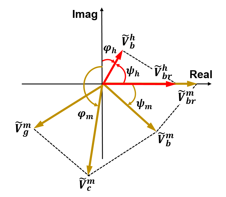
Figure 1: Cavity voltage phasors. $\widetilde{V}^{h}_{b}$ and $\widetilde{V}^{m}_{b}$ are the beam loading voltage phasors of HHC and MC, respectively. $\widetilde{V}^{m}_{g}$ is the generator voltage phasor of MC, and $\widetilde{V}^{m}_{c}=\widetilde{V}^{m}_{b}+\widetilde{V}^{m}_{g}$ is the total voltage phasor of MC.

The resonant modes in RF cavities are in general described as the R-L-C parallel circuit, which have the same impedance form as

$$Z(\omega)=\frac{R}{1+iQ(\frac{\omega_{r}}{\omega}-\frac{\omega}{\omega_{r}})},$$ (1)

where ($R$, $Q$, $\omega_{r}$) are the characteristic parameters of the resonant mode, representing the shunt impedance, quality factor, and angular resonant frequency, respectively. Note that the shunt impedance and quality factor should be considered as loaded values if the cavity has a power coupler.

For the fundamental mode, under uniform filling patterns, the beam-induced stationary voltage phasor is well-known as

$$\widetilde{V}_{b}=2\widetilde{F}I_{0}R\cos{(\psi)}e^{j\psi},$$ (2)

where $\widetilde{F}$ is the complex bunch form factor, $I_{0}$ is the average beam current, and $\psi$ is the detuning phase, which can be computed by

$$\tan{(\psi)}=\frac{2Q\Delta\omega}{\omega_{r}},$$ (3)

where $\Delta\omega=\omega_{r}-\omega_{rf}$ is the angular detuning frequency.

As for the passive HHC, its voltage amplitude is $2FI_{0}R\cos{(\psi_{h})}$ with $F$ being the bunch form factor amplitude, and in sine convention, its reference phase is $\varphi_{h}=\psi_{h}+\varphi_{F}-\pi/2$ with $\varphi_{F}$ being the bunch form factor phase. The HHC voltage is given as

$$V^{h}_{b}(\varphi)=2FI_{0}R\cos{(\psi_{h})}\sin{(n\varphi+\varphi_{h})}.$$ (4)

For MC, its voltage contributed by both the beam and generator current can be given as

$$V^{m}_{c}(\varphi)=V_{m}\sin{(\varphi+\varphi_{m})},$$ (5)

where $V_{m}$ and $\varphi_{m}$ are the amplitude and reference phase, respectively.

It should be noted that for the double RF system, Eq. (4) is commonly used to analytically calculate the beam equilibrium distribution, which can be further used for instability analysis. However, it will be shown later that Eq. (4) only includes the long-range effect of beam-fundamental mode interaction and excludes the short-range effect. In some cases where the short-range effect is sufficiently strong, it can also have a significant impact on the beam equilibrium distribution, which in turn affects the instability evolution and requires a special attention.

II.2 Long-range effect

As aforementioned, we are confined to the case of uniform filling patterns. Assuming that the ring has $h$ buckets which are filled with $m$ equally spaced bunches ($h/m$ is an integer). We further assume that these bunches have identical normalized equilibrium distribution of $\rho(\tau)$. Let us first deduce the cavity voltage induced by a single passage of one bunch through the cavity. As is well known that this voltage is equivalent to He21

$$\widetilde{V}_{0}=\frac{q\omega_{r}R}{Q}\int_{-\infty}^{\infty}\rho(\tau)e^{(-j+\frac{1}{2Q})\omega_{r}\tau}\,d\tau,$$ (6)

where $q$ is the bunch charge. The integral part is simply denoted by $\widetilde{F}=\int_{-\infty}^{\infty}\rho(\tau)e^{(-j+\frac{1}{2Q})\omega_{r}\tau}\,d\tau$, being the complex bunch form factor. Then Eq. (6) can be simplified to

$$\widetilde{V}_{0}=\frac{\widetilde{F}q\omega_{r}R}{Q}.$$ (7)

After the Nth passage of the bunches, the beam-induced cavity voltage can be expressed as

$$\widetilde{V}_{N}=\widetilde{F}\frac{q\omega_{r}R}{Q}\sum\limits^{N}_{i=0}e^{(j-1/2Q)\omega_{r}T_{0}i/m},$$ (8)

where $T_{0}$ is the revolution time. Note that $\widetilde{V}_{N}$ will converge to a certain value as $N$ approaches infinity. With $\alpha=(j-1/2Q)\omega_{r}T_{0}$, Eq. (8) can be simplified as

$$\widetilde{V}_{N}=\frac{\widetilde{F}q\omega_{r}R/Q}{1-e^{\alpha/m}}.$$ (9)

Now, we will distinguish between the long-range and short-range effects of beam-resonant mode interaction. The long-range effect refers to the cavity voltage excited and accumulated by the previous bunch of passages through the RF cavity. For a certain bunch, when it passes through the RF cavity, the steady-state cavity voltage it sees has undergone a period of evolution (decaying and rotation) compared to when the previous bunch passed through. This period is equal to the interval time of $T_{0}/m$ between adjacent bunches. Therefore, the cavity voltage phasor seen by the present bunch has become

$$\widetilde{V}_{L}=\frac{\widetilde{F}q\omega_{r}R/Qe^{\alpha/m}}{1-e^{\alpha/m}}=\frac{\widetilde{F}q\omega_{r}R/Q}{e^{-\alpha/m}-1}.$$ (10)

When m is much larger than 1, we have

$$e^{-\alpha/m} =e^{-j\omega_{r}T_{0}/m}e^{\frac{\omega_{r}T_{0}}{2Qm}}$$ (11)

$$=e^{-j\Delta\omega T_{0}/m}e^{\frac{\omega_{r}T_{0}}{2Qm}}$$

$$\approx 1-j\Delta\omega T_{0}/m+\frac{\omega_{r}T_{0}}{2Qm}.$$

Substituting Eq. (11) into Eq. (10), it gives

$$\widetilde{V}_{L} \approx\frac{\widetilde{F}mq\omega_{r}R/Q}{\frac{\omega_{r}T_{0}}{2Q}-j\Delta\omega T_{0}}$$ (12)

$$=\frac{2\widetilde{F}Rmq/T_{0}}{1-j2Q\Delta\omega/\omega_{r}}$$

$$=2\widetilde{F}I_{0}R\cos{(\psi)}e^{j\psi}.$$

where $\psi=\arctan(\frac{2Q\Delta\omega}{\omega_{r}})$, being the detuning phase. Note that Eq. (12) is the same as Eq. (2), indicating that Eq. (2) only represents the long-range effect of beam-fundamental mode interaction. It should also be noted that when $m$ approaches 1, the approximation process in Eq. (11) will introduce a certain error.

II.3 Short-range effect

The short-range effect can be described directly with the corresponding Green’s wakefield function of resonant modes Palumbo22

$$W_{SR}(\tau)=\frac{\omega_{r}R}{Q}e^{-\frac{\omega_{r}\tau}{2Q}}[\cos(\omega_{n}\tau)-\frac{\omega_{r}}{2Q\omega_{n}}\sin(\omega_{n}\tau)]H(\tau),$$ (13)

where $H(\tau)$ is the Heaviside step function, and $\omega_{n}$ is written as

$$\omega_{n}=\frac{\omega_{r}\sqrt{4Q^{2}-1}}{2Q}.$$ (14)

For a narrowband resonator with large $Q$ value, its wake function can be simplified as

$$W_{SR}(\tau)=\frac{\omega_{r}R}{Q}e^{-\frac{\omega_{r}\tau}{2Q}}\cos(\omega_{r}\tau)H(\tau).$$ (15)

Note that Eq. (15) can be used to describe the beam-cavity resonant mode interaction for one bunch at the present passage. It is clear that the short-range wakefield strength fully depends on the product of $R/Q$ and $\omega_{r}$, indicating that those resonant modes having high $R/Q\times\omega_{r}$ possibly lead to a strong effect.

II.4 Beam equilibrium distribution

We emphasize here that the long-range and the short-range effects of beam-cavity resonant mode interaction have been distinguished as mentioned above. For those light sources utilizing the double RF system, the steady-state total RF voltage corresponding to the long-range is given as

$$V_{T}(\tau)=V_{m}\sin(\omega_{rf}\tau+\varphi_{m})+kV_{m}\sin(n\omega_{rf}\tau+\varphi_{h}),$$ (16)

where $k$ is the voltage ratio of HHC to MC.

The optimum lengthening condition can be reached by setting the first and second derivatives of the total RF voltage to zero. Under this condition, the RF potential is flat at the center, so it is also called the flat-potential condition (FP). To keep it fulfilled, we have Byrd02

$$k_{fp}=\sqrt{\frac{1}{n^{2}}-\frac{1}{n^{2}-1}\Big{(}\frac{U_{0}}{eV_{m}}\Big{)}^{2}},$$ (17)

$$\tan{(\varphi_{h,fp})}=-\frac{nU_{0}}{eV_{m}}\frac{1}{\sqrt{(n^{2}-1)^{2}-\Big{(}\frac{n^{2}U_{0}}{eV_{m}}\Big{)}^{2}}},$$ (18)

$$\sin{(\varphi_{m,fp})}=\frac{n^{2}}{n^{2}-1}\frac{U_{0}}{eV_{m}},$$ (19)

with $\varphi_{m,fp}$ and $\varphi_{h,fp}$ are the flat-potential synchronous phases of the main and harmonic cavities, respectively, and $k_{fp}$ is the flat-potential voltage ratio of HHC to MC. Note that the above three parameters are obtained in the absence of the short-range effects, so they are unperturbed values.

The corresponding RF potential can be written as

$$\Phi_{RF}(\tau)=\frac{eV_{m}}{2\pi hE_{0}\alpha_{c}\sigma_{\delta}^{2}}\{\cos(\varphi_{m})-\cos(\omega_{rf}\tau+\varphi_{m})+$$ (20)

$$\frac{k}{n}[\cos(\varphi_{h})-\cos(n\omega_{rf}\tau+\varphi_{h})]-\frac{U_{0}\omega_{rf}\tau}{eV_{m}}\},$$

where $h$ is the harmonic number, $E_{0}$ is the beam energy, $\alpha_{c}$ is the momentum compaction factor, $\sigma_{\delta}$ is the rms energy spread, and $U_{0}$ is the energy loss per turn.

The short-range potential can be given as

$$\Phi_{SR}(\tau)=\frac{q}{E_{0}T_{0}\alpha_{c}\sigma_{\delta}^{2}}\int_{0}^{\tau}d\tau^{\prime}\int_{-\infty}^{\infty}\rho(\tau^{\prime\prime})W_{SR}(\tau^{\prime}-\tau^{\prime\prime})\,d\tau^{\prime\prime},$$ (21)

where $q$ is the bunch charge and $\rho(\tau)$ is the normalized density distribution. $W_{SR}(\tau)$ can be treated as the superposition of the different short-range potentials if multiple resonant modes need to be considered.

The total longitudinal potential is the sum of the long- and short-range potentials

$$\Phi_{T}(\tau)=\Phi_{RF}(\tau)+\Phi_{SR}(\tau).$$ (22)

Then the bunch equilibrium density distribution can be computed with

$$\rho(\tau)=\frac{e^{\Phi_{T}(\tau)}}{\int_{-\infty}^{\infty}e^{\Phi_{T}(\tau)}\,d\tau}.$$ (23)

Eqs. (20)-(23) exactly form the well-known Haïssinski equation Haissinski23 , and the equilibrium density distribution needs to be iteratively solved. This solution is simple and not time-consuming, after all, only a single bunch needs to be calculated for the uniform filling case. While for arbitrary filling cases, there are several existing self-consistent algorithms available for use He21 ; Warnock24 .

We note from Eq. (21) that the strength of the short-range potential is proportional to the bunch charge. Therefore, for those light source storage rings operated in timing mode with high-charged bunches, the short-range potential may significantly affect the bunch equilibrium distribution.

III Influence of the short-range potential on bunch lengthening

The HALF storage ring Bai25 is taken as an example to illustrate the influence of the short-range potential on bunch lengthening. Table 1 shows the HALF main parameters including the double RF cavities and the corresponding RF voltages and phases under the well-known flat-potential condition. It is emphasized that we only consider the bunch distribution determined by the beam-cavity fundamental mode interaction. In addition, four cases are considered: (i) ignoring the short-range potentials (SRP); (ii) considering only the SRP from MC; (iii) considering only the SRP from HHC; (iv) considering the SRPs from both the main and harmonic cavities. For the above cases, the resulting rms bunch length as a function of the bunch charge is illustrated in Fig. 2. It can be seen that the SRPs from the double RF cavities will continually deteriorate the bunch lengthening as increasing the bunch charge. In addition, it can be seen that the influence of HHC is more significant because compared to MC, HHC has a stronger short-range potential (its $R/Q$ is slightly smaller, but its frequency is three times higher than that of MC).

Table 1: Main parameters of HALF used for bunch lengthening calculation.

Parameter	Value
Energy	2.2 GeV
Circumference	479.86 m
Current	350 mA
Momentum compaction	$9.4\times 10^{-5}$
Harmonic number	800
Radiation energy loss per turn	400 keV
RMS energy spread	$7.44\times 10^{-4}$
Bunch charge (completely filling)	0.7 nC
500 MHz MC $R/Q$	45 $\Omega$
500 MHz MC loaded $Q$	$1\times 10^{5}$
3rd HHC $R/Q$	39 $\Omega$
3rd HHC loaded $Q$	$2\times 10^{8}$
MC voltage amplitude	1200 kV
MC voltage phase (FP)	158.0 deg
HHC voltage amplitude (FP)	374.2 kV
HHC voltage phase (FP)	-7.68 deg

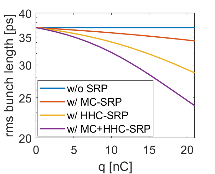
Figure 2: RMS bunch length as a function of the bunch charge.

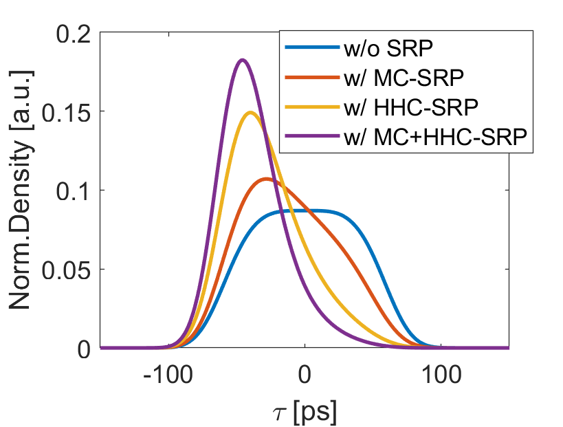
Figure 3: Bunch profiles for the case of assuming a high bunch charge of 20 nC.

Figure 3 shows the corresponding bunch equilibrium profiles for a high bunch charge of 20 nC. Under such a high-charge scenario, the SRPs of the double RF cavities are strong enough to cause the flat potential well distortion, making the beam distribution no longer symmetrical and lean forward associated with reducing the bunch length. It should be pointed out that for HALF with at least 80 percent filling rate, the actual bunch charge is generally less than 1 nC, so it can be expected that the influence of the SPRs from the RF cavities on bunch equilibrium profiles can be ignored fully.

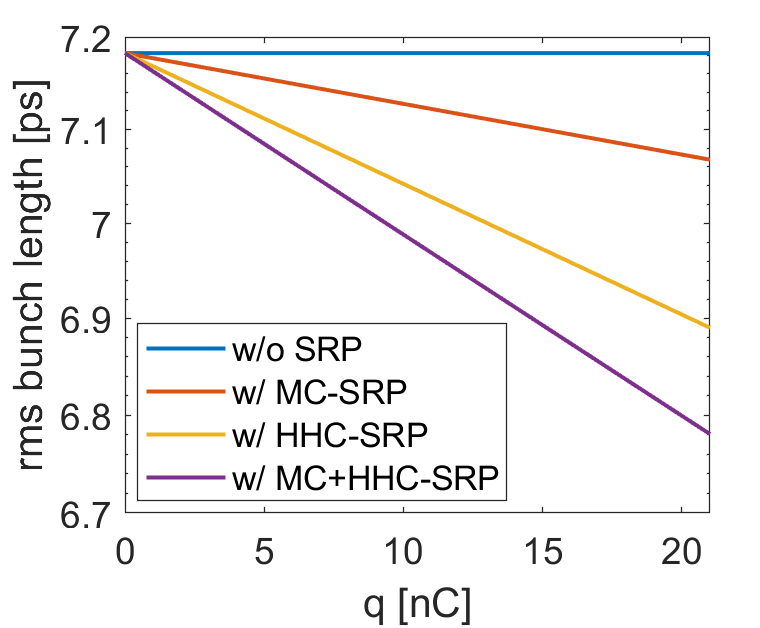
Figure 4: RMS bunch length as a function of the bunch charge.

For the case of parking the harmonic cavity (that is, minimizing its voltage), the resulting bunch length as a function of the bunch charge is shown in Fig. 4. The same four cases as aforementioned are considered. It can be seen that the SRPs also reduce the bunch length as increasing the bunch charge. Nevertheless, the reduction in bunch length is not so critical with respect to those shown in Fig. 2.

In the above analysis, it is assumed that $R/Q$ remains constant and the bunch charge is increased to give prominence to the short-range potential. It should be pointed out that the short-range potential strength is proportional to the product of the bunch charge and $R/Q$. Therefore, in case of a small bunch charge but large $R/Q$, such as when there are multiple cavities, the short-range potential can be strong enough to significantly affect the bunch lengthening under the flat-potential condition.

The short-range potential is also related to the quality factor and resonant frequency, whose influences on the bunch lengthening will be discussed separately as follows.

III.1 Quality factor

For RF cavities, it should be noted that the SRP is related to the loaded quality factor (not the intrinsic quality factor), which can be changed significantly due to the different coupling coefficient settings. It then raises a question: will the change in $Q$ value affect the SRPs? Figures 5 and 6 respectively show the wakefield function in a short range and the corresponding bunch equilibrium profiles for the case of three $Q$ values of HHC fundamental mode. It can be seen that even when the $Q$ value is reduced to 20, it only slightly affects the short-range wakefield, thus hardly affect the bunch equilibrium profiles.

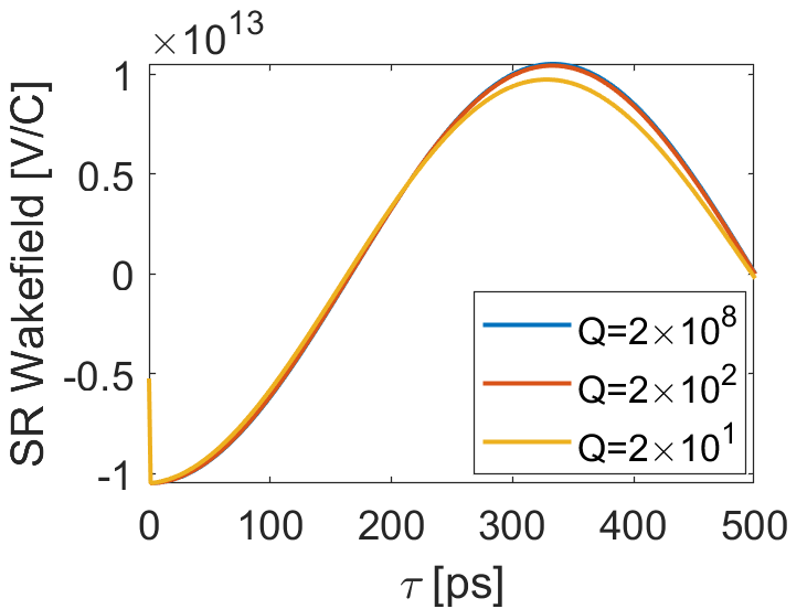
Figure 5: The short-range wakefield for the harmonic cavity with different Q values.

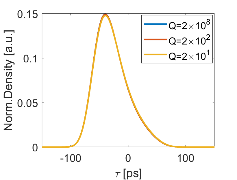
Figure 6: Bunch profiles for the case of assuming a high bunch charge of 20 nC.

III.2 Resonant frequency

It has been shown the influence of the SRPs from the 500 MHz main and 1500 MHz harmonic cavities on the bunch lengthening, and it can be seen that HHC SRP has a more significant impact on the bunch lengthening due to its higher resonant frequency compared to MC. Considering the parasitic modes in RF cavities, if their $R/Q$ is large, their SRPs can also affect the bunch lengthening. Therefore, it is necessary to assess the influence of the SRP at other resonant frequencies. Here, we assume a single resonant mode has $R/Q$ of 39 $\Omega$ and $Q$ of $2\times 10^{8}$, which are the same as those of the HALF HHC. The cases of six frequencies uniformly spaced in the range of 1$\sim$6 GHz are investigated. The resulting bunch length versus the bunch charge is shown in Fig. 7. It can be seen that the SRP can reduce or enhance the bunch lengthening, which depends strongly on the resonant frequency. For HALF, it can be concluded that the SRP within 3 GHz will deteriorate the bunch lengthening; while for the case of higher than 4 GHz, it can enhance the bunch lengthening and even form a double-hump bunch profile, as shown in Fig. 8

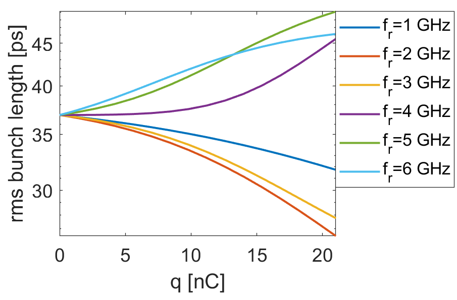
Figure 7: RMS bunch length as a function of the bunch charge. The legend gives the resonant frequency.

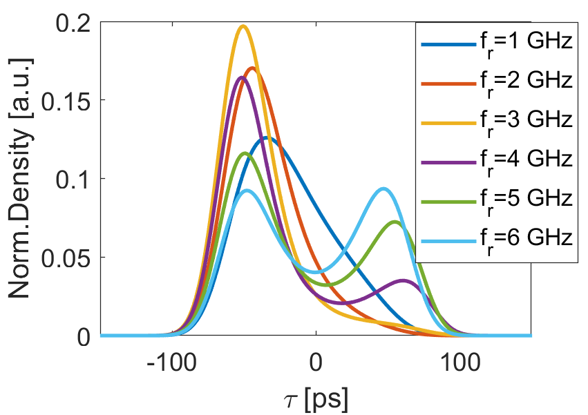
Figure 8: Bunch profiles for the case of assuming a high bunch charge of 20 nC. The legend gives the resonant frequency.

The above results indicate that, for abundant parasitic modes in RF cavities with large total $R/Q$ values, even if they are heavily damped, the corresponding SRPs can still impose a significant influence on the bunch equilibrium distribution under the optimum lengthening condition.

In order to show the significant influence of the SRP on bunch equilibrium distribution, we assume a non-practical case of high bunch charge for HALF. Based on such an assumed scenario, we are able to analyze how the SRP affects the bunch lengthening. Obviously, the HALF bunch lengthening is not troubled by the SRPs of resonant modes in RF cavities. However, for those synchrotron light storage rings requiring multiple RF cavities with large $R/Q$ and being necessarily in timing-mode operation with high bunch charge, it is a must to consider the SRP influence, especially when trying to reach the optimum bunch lengthening with the help of HHC.

IV Application to the PETRA-IV storage ring

In Table 2 we summarize the information of bunch charge, and total $R/Q$ of main and harmonic cavities for the 4th generation of high energy synchrotron light sources, including HEPS Zhang26 , APS-U APSU09 , ESRF-EBS Jacob27 , and PETRA-IV Ebert28 . Considering the SRPs contributed from both main and harmonic cavities, it can be found that PETRA-IV has the strongest SRPs from the double RF system. As a consequence, it is expected that the SRPs of PETRA-IV are likely to impact the bunch lengthening significantly.

Table 2: Bunch charge and cavity parameters of four high-energy synchrotron light sources.

Light source	Timing-mode bunch charge	MC total $R/Q$ @ Frequency	HHC total $R/Q$ @ Frequency
HEPS	14.4 nC	348 $\Omega$ @ 166.6 MHz	95 $\Omega$ @ 500 MHz
APS-U	15.3 nC	1248 $\Omega$ @ 352 MHz	52 $\Omega$ @ 1408 MHz
ESRF-EBS	28 nC	943 $\Omega$ @ 352 MHz	356 $\Omega$ @ 1409 MHz
PETRA-IV	7.68 nC	2757 $\Omega$ @ 500 MHz	2117 $\Omega$ @ 1500 MHz

IV.1 Bunch lengthening under the optimum lengthening setting

Figure 9 shows the bunch equilibrium distributions for PETRA-IV in the case of the optimum lengthening setting of HHC voltage, which are obtained using the parameters listed in Table 2 and in Ref. Agapov29 . Four cases abbreviated as the legends shown in Fig. 2 are considered, same as those done for HALF in Fig. 2. Without the SRP, the optimum-lengthening rms bunch length is 40.2 ps. The inclusion of the SRPs from MC and HHC can reduce the rms bunch length down to 13.6 ps. Figure 10 shows the corresponding potential distributions, indicating that the SRP causes a significant distortion to the flat RF potential. It also means that the bunch lengthening is not optimum even if the harmonic voltage is set to meet the so-called optimum lengthening condition.

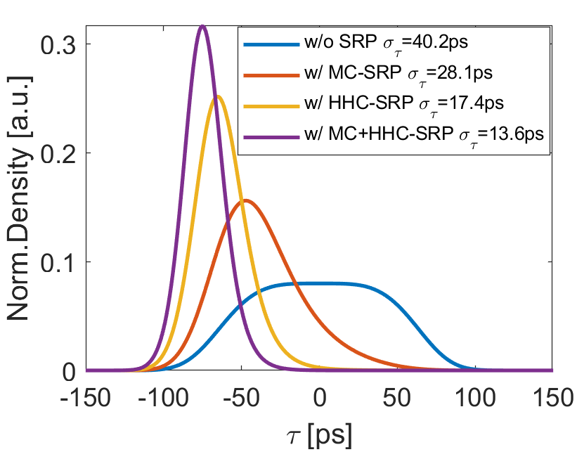
Figure 9: Bunch profiles for PETRA-IV in the case of flat-potential HHC voltage setting and maximum bunch charge required for the timing-mode operation.

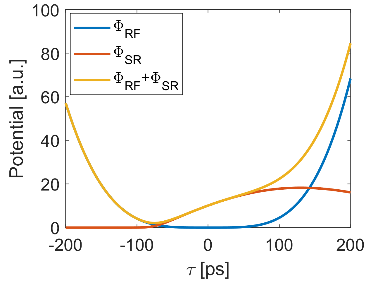
Figure 10: Potential distribution.

IV.2 Optimization of bunch lengthening

Actually, the bunch lengthening can be improved by optimizing the harmonic voltage setting compared to utilizing directly the flat-potential setting. For the double RF system with given main voltage and cavity parameters, the adjustable parameters are the harmonic cavity voltage and phase. The optimization with only two variables can be performed easily based on parameter scanning. To facilitate this scanning, we introduce two coefficients of $k_{v}$ and $k_{\varphi}$, which are the ratio of HHC voltage and phase with respect to those under the flat-potential condition. Consequently, $k_{v}$ and $k_{\varphi}$ are scanned to find the optimum bunch lengthening.

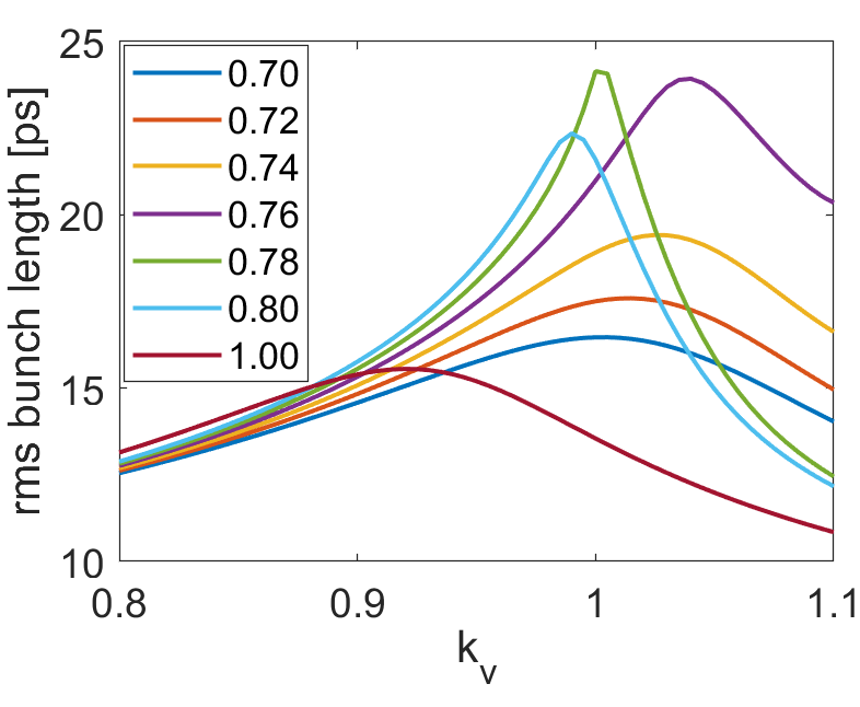
Figure 11: The rms bunch length obtained by scanning the HC $k_{v}$ and $k_{\varphi}$. The legend gives the value of $k_{\varphi}$

Figure 11 demonstrates the scanning results, where $k_{v}$ and $k_{\varphi}$ are confined in the range of 0.8-1.1 and 0.7-0.8, respectively. To facilitate the comparison with the original flat-potential setting, the case of $k_{\varphi}$=1 is also shown in Fig. 11. It is very clear that there is the maximum bunch lengthening existed for the case of $k_{\varphi}$ in the range of 0.76-0.78. After more precise scanning, a near optimum setting of $k_{v}$=1.02 and $k_{\varphi}$=0.765 was determined. Under this setting, it was found two equilibrium solutions with rms bunch lengths of 25.7 ps and 23.2 ps, as shown in Fig. 12. The former solution is obtained by scanning $k_{v}$ from 1.0 to 1.02, and the latter is from 1.1 to 1.02. While the tracking results are consistent with the former when tracking with an initial Gaussian bunch distribution. It means that the rms bunch length can exceed 25 ps, almost twice that in the flat-potential setting.

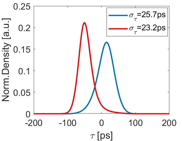
Figure 12: Bunch profiles for the case of $k_{v}$=1.02 and $k_{\varphi}$=0.765. There are two equilibrium solutions, and the legend gives the corresponding rms bunch length.

Note that in the above optimization, only the SRPs of RF cavity fundamental modes are considered. When it is necessary to consider parasitic modes with large $R/Q$, or the total broadband impedance, or both, we can still follow the above optimization idea that optimizing HHC voltage and phase to maximize the equilibrium bunch length.

V Conclusion

In this paper, we studied the short-range effect of resonant mode impedances on bunch lengthening. It was found that (i) the short-range potentials impact slightly on the bunch equilibrium distribution in absence of harmonic cavities; (ii) in the case of optimum lengthening setting of the harmonic cavity, the short-range potentials contributed by the fundamental mode impedances of main and harmonic cavities can significantly reduce the bunch lengthening; (iii) parasitic modes have short-range potentials independent of $Q$, which can also affect much the bunch lengthening if their $R/Q$ is large; (iv) in the case of timing-mode operation with high bunch charge and multiple RF cavities with large total $R/Q$, the influence of the short-range potentials of all resonant modes in RF cavities has to be taken into account in the accurate evaluation of the beam equilibrium distribution; (v) in the case of strong short-range potentials of resonant modes, the conventional optimum lengthening setting cannot achieve the optimum lengthening, and there are other harmonic cavity parameters to maximize the bunch lengthening. The above findings are of importance for the synchrotron light sources that use multiple RF cavities and need to pursue optimum lengthening in case of high bunch charge filling.

- (1) R. Nagaoka, K. L. F. Bane, Collective effects in a diffraction-limited storage ring, J. Synchrotron Radiat. 21, 937 (2014).
- (2) J. M. Byrd and M. Georgsson, Lifetime increase using passive harmonic cavities in synchrotron light sources, Phys. Rev. ST Accel. Beams 4 030701 (2001).
- (3) F. J. Cullinan, Å. Andersson and P. F. Tavares, Review of harmonic cavities in fourth-generation storage rings, in Proceedings of the FLS2023, Luzern, Switzerland, (JACOW, Luzern, Switzerland, 2023), M02L3.
- (4) T. L. He, Z. H. Bai, G. Y. Feng, W. W. Li, W. M. Li, G. W. Liu, L. Wang, H. L. Xu, and S. C. Zhang, Bunch lengthening of the HALF storage ring in the presence of passive harmonic cavities, in Proceedings of the IPAC2021, Campinas, SP, (JACoW, Campinas, SP, Brazil, 2021), pp. 2082-2085, TUPAB265.
- (5) P. F. Tavares, S. C. Leemann, M. Sjöström and Å. Andersson, The MAX IV storage ring project, J. Synchrotron Radiat. 21, 862 (2014).
- (6) N. Carmignani, J. Jacob, B. Nash and S. White, Harmonic RF System for the ESRF EBS, in Proceedings of the IPAC2017, Copenhagen, Denmark, (JACOW, Copenhagen, Denmark, 2017), pp. 3684-3687 THPAB003.
- (7) C. G. Schroer, I. Agapov, W. Brefeld, R. Brinkmann, Y.-C. Chae, H.-C. Chao, M. Eriksson, J. Keil, X. Nuel Gavaldà, R. Röhlsberger, O. H. Seeck, M. Sprung, M. Tischer, R. Wanzenberg and E. Weckert, PETRA IV: the ultralow-emittance source project at DESY, J. Synchrotron Radiat. 25, 1277 (2018).
- (8) Y. Jiao, G. Xu, X. H. Cui, Z. Duan, Y. Y. Guo, P. He, D. H. Ji, J. Y. Li, X. Y. Li, C. Meng, Y. M. Peng, S. K. Tian, J. Q. Wang, N. Wang, Y. Y. Wei, H. S. Xu, F. Yan, C. H. Yu, Y. L. Zhao, Q. Qin, The HEPS project, J. Synchrotron Radiat. 25, 1611 (2018).
- (9) Advanced Photon Source Upgrade Project Final Design Report, https://publications.anl.gov/anlpubs/2019/07/153666.pdf.
- (10) A. W. Chao, Physics of Collective Beam Instabilities in High Energy Accelerators, (Wiley, New York, 1993) p. 162.
- (11) T. L. He, W. W. Li, Z. H. Bai, W. M. Li, Mode-zero Robinson instability in the presence of passive superconducting harmonic cavities, Phys. Rev. Accel. Beams 26, 064403 (2023).
- (12) M. Venturini, Passive higher-harmonic rf cavities with general settings and multibunch instabilities in electron storage rings, Phys. Rev. Accel. Beams 21 114404 (2018).
- (13) T. He, Novel perturbation method for judging the stability of the equilibrium solution in the presence of passive harmonic cavities, Phys. Rev. Accel. Beams 25 094402 (2022).
- (14) T. He, W. Li, Z. Bai, and L. Wang, Periodic transient beam loading effect with passive harmonic cavities in electron storage rings, Phys. Rev. Accel. Beams 25 024401 (2022).
- (15) N. Yamamoto, T. Yamaguchi, P. Marchand, A. Gamelin, and R. Nagaoka, Stability survery of a double RF system with RF feedback loops for bunch lengthening in a low-emittance synchrotron ring, in Proceedings of the IPAC2023, Venice, Italy, (JACOW, Venice, Italy, 2023), pp. 3451-3454, WEPL161.
- (16) A. Gamelin, W. Foosang, P. Marchand, R. Nagaoka, and N. Yamamoto, Beam dynamics with a superconducting harmonic cavity for the SOLEIL Upgrade, in Proceedings of the IPAC2022, Bangkok, Thailand, (JACOW, Bangkok, Thailand, 2022), pp. 2229-2232, WEPOMS003.
- (17) I. Bellafont, P. Solans, and F. Pérez, Longitudinal beam dynamics studies with a third harmonic RF system for ALBA-II, in Proceedings of the IPAC2023, Venice, Italy, (JACOW, Venice, Italy, 2023), pp. 3487-3490, WEPL179.
- (18) F. J. Cullinan, Å. Andersson, and P. F. Tavares, Harmonic-cavity stabilization of longitudinal coupled-bunch instabilities with a nonuniform fill, Phys. Rev. Accel. Beams 23 074402 (2020).
- (19) P. F. Tavares, F. J. Cullinan, Å Andersson, D. Olsson, and R. Svärd, Beam-based characterization of higher-order-mode driven coupled-bunch instabilities in a fourth-generation storage ring, Nucl. Instrum. Methods Phys. Res., Sect. A 1021, 165945 (2022).
- (20) K. Y. Ng, Physics of Intensity Dependent Beam Instabilities, (World Scientific Publishing, Singapore, 2006) pp. 241-253.
- (21) T. L. He, W. W. Li, Z. H. Bai, and L. Wang, Longitudinal equilibrium density distribution of arbitrary filled bunches in presence of a passive harmonic cavity and the short range wakefield, Phys. Rev. Accel. Beams 24 044401 (2021).
- (22) L. Palumbo, V. G. Vaccaro, and M. Zobov, CERN Report No. CERN 95-06, Geneva, Switzerland, 1995, pp. 331–390.
- (23) J. Haissinski, Exact longitudinal equilibrium distribution of stored electrons in the presence of self-fields, Neural Comput. 18B (1) (1973).
- (24) R. Warnock, Equilibrium of an arbitrary bunch train with cavity resonators and short range wake: Enhanced iterative solution with Anderson acceleration, Phys. Rev. Accel. Beams 24 104402 (2021).
- (25) Z. Bai, G. Feng, T. He, W. Li, W. Li, G. Liu, J. Tang, L. Wang, P. Yang, and S. Zhang, Progress on the Storage ring physics design of Hefei Advanced Light Facility (HALF), in Proceedings of the IPAC2023, Venice, Italy, (JACOW, Venice, Italy, 2023), pp. 1057-1060, MOPM038.
- (26) P. Zhang, J. Dai, Z. Deng, L. Guo, T. Huang, D. Li, J. Li, Z. Li, H. Lin, Y. Luo, Q. Ma, F. Meng, Z. Mi, Q. Wang, H. Xu, X. Zhang, F. Zhao and H. Zheng, Radio-frequency system of the high energy photon source, Radiat Detect Technol Methods 7 159–170 (2023).
- (27) J. Jacob, P. Borowiec, A. D’Elia, G. Gautier, and V. Serrière, ESRF-EBS 352.37 MHz Radio Frequency System, in Proceedings of the IPAC2021, Campinas, SP, Brazil, (JACOW, Campinas, SP, Brazil, 2021), pp. 3487-3490, MOPAB108.
- (28) M. Ebert, Proposal of an RF system for PETRA IV, DESY, Technical Note 19-03, April 2019.
- (29) I. Agapov, S. Antipov, R. Bartolini, R. Brinkmann, Y.-C. Chae, D. Einfeld, T. Hellert, M. Hüening, M. Jebramcik, J. Keil, C. Li, R. Wanzenberg, PETRA IV Storage Ring Design, in Proceedings of the IPAC2022, Bangkok, Thailand, (JACOW, Bangkok, Thailand, 2022), pp. 1431-1434, TUPOMS014.