NeISF: Neural Incident Stokes Field for Geometry and Material Estimation

Abstract

Multi-view inverse rendering is the problem of estimating the scene parameters such as shapes, materials, or illuminations from a sequence of images captured under different viewpoints. Many approaches, however, assume single light bounce and thus fail to recover challenging scenarios like inter-reflections. On the other hand, simply extending those methods to consider multi-bounced light requires more assumptions to alleviate the ambiguity. To address this problem, we propose Neural Incident Stokes Fields (NeISF), a multi-view inverse rendering framework that reduces ambiguities using polarization cues. The primary motivation for using polarization cues is that it is the accumulation of multi-bounced light, providing rich information about geometry and material. Based on this knowledge, the proposed incident Stokes field efficiently models the accumulated polarization effect with the aid of an original physically-based differentiable polarimetric renderer. Lastly, experimental results show that our method outperforms the existing works in synthetic and real scenarios.

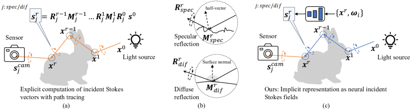
Figure 2: Concept of our incident Stokes fields. The orange paths are explicitly computed, while the blue paths are implicitly represented. (a) In the traditional path tracer, the incident Stokes vectors are computed by the recursive multiplication of Stokes vectors, rotation Mueller matrices, and pBRDF Mueller matrices. (b) The diffuse and specular pBRDF matrices have different reference frames. Thus, the rotation matrices should be treated separately. (c) Given the positions of the interaction points and the directions of the incident light, we use MLPs to implicitly record the already-rotated incident Stokes vectors of diffuse and specular components, separately.

1 Introduction

Inverse rendering aims at decomposing the target scene into parameters such as geometry, material, and lighting. It is a long-standing task for computer vision and computer graphics and has many downstream tasks, such as relighting, material editing, and novel-view synthesis. The main challenge of inverse rendering is that many combinations of the scene parameters can express the same appearance, called the ambiguity problem. Solutions to the ambiguity can be roughly divided into two categories: simplifying the scene and utilizing more information. For the first group, some studies assume a Lambertian Bidirectional Reflectance Distribution Function (BRDF) [71], a single point light source [18], or a near-planer geometry [46]. For the second group, additional information such as multiple viewpoints [33], additional illuminations [11], multi-spectral images [40], depth information [36], and polarization cues [94] has been extensively explored.

Most of the aforementioned methods use explicit representations of scene parameters. On the other hand, Neural Radiance Fields (NeRF) [58] shows the successful use of implicit representations. Although NeRF achieves remarkable performance on novel-view synthesis, it does not decompose the scene into the parameters. Thus, many approaches try to extend the NeRF representation to solve inverse rendering, and solutions to the ambiguity problem can still be categorized into the two groups stated above. For the first group, assumptions such as a smooth roughness field [82], low roughness [74], known lighting [73, 81], single light bounce [7, 8], collocated flashlight [90], or a Lambertian surface [89] are proposed to stabilize the training. However, these assumptions severely limit the scope of target scenes. For the second group, various types of cues such as depth images [1], azimuth maps [13], multiple lights [42, 52] and multi-spectral information [68] are investigated. Additionally, polarization is also examined in this group. To our knowledge, PANDORA [17] first combines the implicit representations and polarization cues for the diffuse-specular reflection separation and the geometry estimation. However, due to the entangled representation of the incident light and surface reflectance, BRDF parameters are not estimated. In addition, they assume a single light bounce and unpolarized incident light. These limitations lead to our key research question: Can polarization cues disambiguate the full NeRF-based inverse rendering?

We propose Neural Incident Stokes Fields (NeISF), an inverse rendering method using polarization cues and implicit representations. It takes multi-view polarized images of a static object with known object masks and camera poses but with unknown geometry, material, and lighting. Based on the implicit representation for the multi-bounced light [82, 89], the proposed incident Stokes fields effectively extend this representation to include the polarization cues. Specifically, instead of explicitly modeling every single light bounce as shown in Fig. 2 (a), we use coordinate-based multi-layer perceptrons (MLPs) to record Stokes vectors of all the second-last bounces (Fig. 2 (c)). After that, we introduce a physically-based polarimetric renderer to compute Stokes vectors of the last bounces using a polarimetric BRDF model proposed by Baek et al. [5] (Baek pBRDF). The challenging part of extending an unpolarized incident light field to a polarized one is that we must ensure that the Stokes vectors are properly rotated to share the same reference frame with the Mueller matrices. Furthermore, the diffuse and specular components have different reference frames, which makes the problem more complicated. This is because the reference frame of diffuse Mueller matrices depends on the surface normal, while the reference frame of specular Mueller matrices depends on the microfacet normal (Fig. 2 (b)). To solve this issue, we propose to implicitly record the rotation of the second-last bounce for the diffuse and specular components separately. More specifically, given the position and direction of the incident light, we use MLPs to record the already rotated Stokes vectors of diffuse and specular components independently. Our light representation is capable of handling challenging scenes including those that have inter-reflections. In addition, the polarization cues can provide a wealth of information on geometry, material, and light, making it easier to solve inverse rendering compared to unpolarized methods. To comprehensively evaluate the proposed approach, we construct two polarimetric HDR datasets: a synthetic dataset rendered by Mitsuba 3.0 [28], and a real-world dataset captured by a polarization camera. Fig. 1 shows that our model outperforms the existing methods. Our contributions are summarized as follows:

• This method introduces a unique representation, which implicitly models multi-bounce polarized light paths with the rotation of Stokes vectors taken into account.

• To perfectly integrate the representation into the training pipeline, we introduce a differentiable physically-based polarimetric renderer.

• Our method achieves state-of-the-art performance on both synthetic and real scenarios.

• Our real and synthetic multi-view polarimetric datasets and implementation are publicly available.

2 Related Works

Inverse Rendering We roughly divide the existing inverse rendering works into two groups, which are learning-based and optimization-based methods. Most of the learning-based inverse rendering works [41, 49, 70, 45, 77, 96, 48, 10, 69, 51] are single-view approaches. They mainly rely on large-scale synthetic training datasets because acquiring the ground truth material, geometry, and lighting parameters is labor-intensive and time-consuming. A well-known problem of using synthetic training data is the domain gap, where the trained model often fails to give reasonable results for the real-world scene. Optimization-based methods [59, 64, 6, 86, 54, 66, 55], also known as analysis by synthesis, are the other direction to solve inverse rendering. The recent breakthrough of optimization-based methods is dominated by the differentiable rendering [62, 44, 88, 87]. Differentiable renderers like Mitsuba [63] are able to backpropagate the gradients to physical parameters even when the light is bounced multiple times. However, it requires a huge computational cost and memory consumption when handling a complex scene. NeRF-based inverse rendering can also be classified as the optimization-based method. Compared to the explicit representation of scene parameters, the compactness and effectiveness of neural implicit representation have been verified. Details will be introduced in the next part.

Neural Implicit Fields NeRF [58] achieved photorealistic performance for novel-view synthesis utilizing the effectiveness of implicit neural representation. However, inverse rendering is not directly supported due to the entangled representation. This limitation has opened up a new research field on neural implicit fields-based inverse rendering.

Some works only focus on geometry estimation. Representative works such as IDR [85], NeuS [76], VolSDF [83], and BakedSDF [84] can be classified into this group. They disentangle the geometry but use an entangled representation of the lighting and material. Attempts to complete the disentanglement have been widely studied. Early works only consider the direct lighting represented by a spherical Gaussian [7, 91], an environment map [92], or split-sum approximation [9, 60]. These direct lighting-based works are not capable of handling complex effects like inter-reflection. Later, several works [78, 47, 93, 29, 79, 95] that also consider indirect lighting have been reported. One simple but efficient solution is Neural Radiosity [23], which records a part of light bounces using MLPs. Inspired by them, many works [82, 89, 24] also use such kind of light representation for inverse rendering. We extend their idea by proposing the neural incident Stokes fields to model the multi-bounced polarimetric light propagation.

Polarization Polarization is one of the properties of electromagnetic waves that specifies the geometrical orientation of the oscillations. An important phenomenon of polarization is that it changes after interacting with objects, providing rich information for a variety of applications including inverse rendering. Since the release of commercial polarization cameras [80], it has become easier to capture polarized images, and polarization research has become more active. Various applications such as the estimation of shape [61, 35, 21, 27, 3, 39, 72, 14, 30, 97], material [2, 19, 26, 4, 20], pose [16, 98, 22], white balance [65], reflection removal [38, 56, 43], segmentation [32, 57, 50], and sensor design [37] have been explored.

So far, attempts to combine NeRF and polarization mainly focused on extending the intensity fields to the polarimetric (pCON [67]) fields or Spectro-polarimetric (NeSpoF [34]) fields for novel-view synthesis. Namely, they do not use polarization for inverse rendering. PANDORA [17] is the first work that combines polarization cues and NeRF for inverse rendering purposes. They train coordinate-based MLPs to estimate normals, diffuse radiance, and specular radiance. After that, the estimated normals, diffuse radiance, and specular radiance are combined by a simplified renderer to generate the outgoing Stokes vectors. The main limitation of PANDORA can be considered as follows. First, it does not support the inverse rendering of BRDF parameters. Because the diffuse and specular radiance entangles the incident light, BRDF, and normals. Second, they assume an unpolarized incident light. This violates the common situation in the real world where the light has already bounced and become polarized before hitting the object. In contrast, the rendering process of our method is physically based, making it possible to fully disentangle the material, geometry, and lighting. Additionally, we do not require an unpolarized incident light assumption.

3 Preliminary

We briefly introduce the mathematics used to describe the polarimetric light propagation, BRDF, and rendering equation. Please refer to the supplementary material for the detailed version.

3.1 Stokes-Mueller multiplication

The polarization state of the light can be represented as a Stokes vector $\mathbf{s}\in\mathbb{R}^{3}$. It has three elements $[s_{0},s_{1},s_{2}]$, where $s_{0}$ is the unpolarized light intensity, $s_{1}$ is the $0^{\circ}$ over $90^{\circ}$ linear polarization, and $s_{2}$ is the $45^{\circ}$ over $135^{\circ}$ linear polarization. We do not consider the fourth dimension representing circular polarization in this paper. The light-object interaction can be expressed by the multiplication of Stokes vectors and Mueller matrices:

$$\mathbf{s}^{\text{out}}=\mathbf{M}\cdot\mathbf{R}\cdot\mathbf{s}^{\text{in}},$$ (1)

where $\mathbf{M}\in\mathbb{R}^{3\times 3}$ is the Mueller matrix representing the optical property of the interaction point, $\mathbf{s}^{\text{in}}$ and $\mathbf{s}^{\text{out}}$ are the incident and outgoing Stokes vectors. $\mathbf{R}\in\mathbb{R}^{3\times 3}$ is the rotation matrix which depends on the relative angle of the reference frames of $\mathbf{s}^{\text{in}}$ and $\mathbf{M}$. It must also be multiplied, as the Stokes-Mueller multiplication is only valid when they share the same reference frame.

3.2 Polarimetric BRDF

In Baek pBRDF, the diffuse and specular components are modeled separately. The diffuse component $\mathbf{M}_{\text{dif}}$ describes the process of transmitting from the outside to inside, subsurface scattering, and transmitting from the inside to outside. It can be formulated as follows:

$$\mathbf{M}_{\text{dif}}=(\frac{\bm{\rho}}{\pi}\cos{\theta_{i}})\mathbf{F}^{T}_{o}\cdot\mathbf{D}\cdot\mathbf{F}^{T}_{i}.$$ (2)

$\bm{\rho}\in\mathbb{R}^{3}$ is the diffuse albedo, $\theta_{i,o}$ denotes the incident / outgoing angle, $\mathbf{D}\in\mathbb{R}^{3\times 3}$ is a depolarizer, and $\mathbf{F}^{T}_{i,o}\in\mathbb{R}^{3\times 3}$ is the Fresnel transmission term. The specular component describes the microfacet surface reflection:

$$\mathbf{M}_{\text{spec}}=\mathbf{k_{s}}\frac{DG}{4\cos{\theta_{o}}}\mathbf{F}^{R},$$ (3)

where $\mathbf{k_{s}}\in\mathbb{R}^{3}$ is the specular coefficient, $D$ is the GGX distribution function [75], $G$ is the Smith function, and $\mathbf{F}^{R}\in\mathbb{R}^{3\times 3}$ is the Fresnel reflection.

3.3 Polarimetric rendering equation

According to Eq. 1, we can obtain the polarimetric version of the Rendering Equation [31]:

$$\mathbf{s}^{\text{cam}}=\mathbf{R}^{\text{cam}}\cdot\int_{\Omega}\mathbf{M}\cdot\mathbf{R}^{\text{in}}\cdot\mathbf{s}^{\text{in}}\,d\bm{\omega_{i}},$$ (4)

where $\mathbf{s}^{\text{cam}}$ is the Stokes vector captured by the camera, $\mathbf{R}^{\text{cam}}$ is the rotation matrix from the Mueller matrix to the camera’s reference frame, rotation matrix $\mathbf{R}^{\text{in}}$ rotates the incident Stokes vector $\mathbf{s}^{\text{in}}$ to the reference frame of Mueller matrix $\mathbf{M}$, $\bm{\omega_{i}}\in\mathbb{R}^{3}$ is the incident direction.

Furthermore, Baek pBRDF handles the rotation matrices of diffuse and specular components in a different manner. Because the reference frame of the diffuse Mueller matrix $\mathbf{M}_{\text{dif}}$ depends on the surface normal, while the reference frame of the specular Mueller matrix $\mathbf{M}_{\text{spec}}$ depends on the microfacet normal (halfway vector) as shown in (Fig. 2 (b)). Thus, for the diffuse component, the Eq. 4 should be rewritten as:

$$\mathbf{s}^{\text{cam}}_{\text{dif}}=\mathbf{R}^{\text{cam}}_{\text{dif}}\cdot\int_{\Omega}\mathbf{M}_{\text{dif}}\cdot\mathbf{R}^{\text{in}}_{\text{dif}}\cdot\mathbf{s}^{\text{in}}\,d\bm{\omega_{i}},$$ (5)

and for the specular component:

$$\mathbf{s}^{\text{cam}}_{\text{spec}}=\int_{\Omega}\mathbf{R}^{\text{cam}}_{\text{spec}}\cdot\mathbf{M}_{\text{spec}}\cdot\mathbf{R}^{\text{in}}_{\text{spec}}\cdot\mathbf{s}^{\text{in}}\,d\bm{\omega_{i}}.$$ (6)

Note that for the specular component, $\mathbf{R}^{\text{cam}}_{\text{spec}}\cdot$ should be placed into the integral, as the microfacet normal changes according to the incident direction $\bm{\omega_{i}}$.

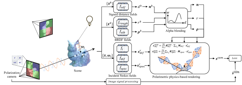
Figure 3: Overview of NeISF. For each interaction point, we use MLPs to implicitly record surface normal n (Sec. 4.2), diffuse albedo $\bm{\rho}$, roughness $r$ (Sec. 4.3), and already-rotated incident Stokes vectors of diffuse $\textbf{s}^{\text{r}}_{\text{dif}}$ and specular $\textbf{s}^{\text{r}}_{\text{spec}}$ components (Sec. 4.4). A physically-based polarimetric renderer is adopted to render the outgoing Stokes vectors $\textbf{s}^{\text{cam}}$ (Sec. 4.5).

4 Our Approach

Our method takes multi-view polarized images, masks, and camera poses as inputs and outputs diffuse albedo, roughness, and surface normal. It supports various downstream tasks including relighting, material editing, and diffuse-specular separation. Details will be introduced in the following subsections, and we show an overview of our method in Fig. 3.

4.1 Assumptions and scopes

We keep the specular coefficient $\bm{k_{s}}=[1,1,1]$. In addition, we assume a constant refractive index $\eta=1.5$, because this is close to the refractive index of common materials such as acrylic glass (1.49), polypropylene plastic (1.49), and quartz (1.458). This work only focuses on object-level inverse rendering, and scene-level inverse rendering is beyond the scope. In addition, Baek pBRDF is only applicable to opaque and dielectric materials, which means objects that include metals, translucent, or transparent parts are not our target objects.

4.2 Signed distance fields

We represent the geometry using a signed distance field net $f_{\text{sdf}}$. Let $\{\mathbf{x}^{k}\}_{k=1}^{N}$ be the $N$ samples along the ray direction:

$$f_{\text{sdf}}(\mathbf{x}^{k})=d^{k},$$ (7)

$d^{k}$ is the signed distance from the nearest surface. The normal of the sampled location $\mathbf{x}^{k}$ can be obtained by calculating the normalized gradient of $f_{\text{sdf}}$:

$$\nabla_{\mathbf{x}^{k}}f_{\text{sdf}}(\mathbf{x}^{k})/||\nabla_{\mathbf{x}^{k}}f_{\text{sdf}}(\mathbf{x}^{k})||_{2}=\mathbf{n}^{k}.$$ (8)

After obtaining all the normals of sampled points, an alpha-blending is required to compute the surface normal of the interaction point. The weight $w^{k}$ of the alpha-blending can be calculated by:

$$w^{k}=T^{k}(1-\exp{(-\sigma^{k}\delta^{k})}),$$ (9)

where $T^{k}=\exp{(-\sum_{j=1}^{k-1}\sigma^{j}\delta^{j})}$, $\delta$ is the distance between two adjacent samples. For the density $\sigma$, we follow the definition of VolSDF [83]:

$$\sigma^{k}=\alpha\Psi_{\beta}(d^{k}),$$ (10)

where $\Psi$ is the cumulative distribution function of the Laplace distribution, $\alpha$ and $\beta$ are two learnable parameters. Then, we compute the alpha-blending to achieve the final surface normal: $\mathbf{n}=\sum_{k=1}^{N}w^{k}\mathbf{n}^{k}$.

4.3 BRDF fields

As the specular coefficient $\bm{k_{s}}$ and refractive index $\eta$ are assumed as constants, we only need to estimate the diffuse albedo $\bm{\rho}$ and roughness $r$. Thus, for each sampled location $\mathbf{x}^{k}$, we estimate:

$$f_{\text{alb}}(\mathbf{x}^{k})=\bm{\rho}^{k},$$ (11)

$$f_{\text{rough}}(\mathbf{x}^{k})=r^{k}.$$ (12)

Similar to the surface normal, the albedo and roughness for the interaction point can also be calculated via alpha-blending: $\bm{\rho}=\sum_{k=1}^{N}w^{k}\bm{\rho}^{k}$, $r=\sum_{k=1}^{N}w^{k}r^{k}$.

		Ours	Ours-no-pol	PANDORA[17]	NeILF++[89]	VolSDF [83]
Bunny	Normal (MAE$\downarrow$)	1.727∘	${}^{\hskip 12.0pt}$3.295∘	${}^{\hskip 12.0pt}$7.769∘	${}^{\hskip 10.79993pt}$4.481∘	${}^{\hskip 10.79993pt}$5.210∘
	Mixed (PSNR$\uparrow$)	36.81	${}^{\hskip 12.0pt}$34.45	${}^{\hskip 12.0pt}$24.62	${}^{\hskip 10.79993pt}$32.08	${}^{\hskip 10.79993pt}$35.08
	Specular (PSNR$\uparrow$)	27.68	${}^{\hskip 12.0pt}$26.91	${}^{\hskip 12.0pt}$20.04	${}^{\hskip 20.64001pt}$-	${}^{\hskip 20.64001pt}$-
	Diffuse (PSNR$\uparrow$)	35.31	${}^{\hskip 12.0pt}$32.93	${}^{\hskip 12.0pt}$24.43	${}^{\hskip 20.64001pt}$-	${}^{\hskip 20.64001pt}$-
	Roughness (SI-L1$\downarrow$)	.0149	${}^{\hskip 12.0pt}$.0244	${}^{\hskip 21.60004pt}$-	${}^{\hskip 20.64001pt}$-	${}^{\hskip 20.64001pt}$-
	Albedo (SI-L1$\downarrow$)	.0372	${}^{\hskip 12.0pt}$.0396	${}^{\hskip 21.60004pt}$-	${}^{\hskip 20.64001pt}$-	${}^{\hskip 20.64001pt}$-
Teapot	Normal (MAE$\downarrow$)	2.541∘	${}^{\hskip 12.0pt}$3.894∘	${}^{\hskip 12.0pt}$6.722∘	${}^{\hskip 10.79993pt}$5.752∘	${}^{\hskip 10.79993pt}$6.375∘
	Mixed (PSNR$\uparrow$)	31.32	${}^{\hskip 12.0pt}$30.23	${}^{\hskip 12.0pt}$22.47	${}^{\hskip 10.79993pt}$25.24	${}^{\hskip 10.79993pt}$28.91
	Specular (PSNR$\uparrow$)	22.50	${}^{\hskip 12.0pt}$21.15	${}^{\hskip 12.0pt}$16.84	${}^{\hskip 20.64001pt}$-	${}^{\hskip 20.64001pt}$-
	Diffuse (PSNR$\uparrow$)	31.97	${}^{\hskip 12.0pt}$30.17	${}^{\hskip 12.0pt}$22.39	${}^{\hskip 20.64001pt}$-	${}^{\hskip 20.64001pt}$-
	Roughness (SI-L1$\downarrow$)	.0172	${}^{\hskip 12.0pt}$.0223	${}^{\hskip 21.60004pt}$-	${}^{\hskip 20.64001pt}$-	${}^{\hskip 20.64001pt}$-
	Albedo (SI-L1$\downarrow$)	.0712	${}^{\hskip 12.0pt}$.0720	${}^{\hskip 21.60004pt}$-	${}^{\hskip 20.64001pt}$-	${}^{\hskip 20.64001pt}$-

Table 1: Results on synthetic dataset. Metrics are computed on 10 test images. The surface normal is evaluated by mean angular error (MAE), and intensity images are evaluated with a peak signal-to-noise ratio (PSNR). Due to the inherent ambiguity of albedo and roughness, we use a scale-invariant L1 error (SI-L1) following IRON [90]. ”Mixed” represents the combination of ”Specular” and ”Diffuse”.

4.4 Incident Stokes fields

As NeILF [82] proposed, the complicated multi-bounced light propagation can be represented as an incident light field. Specifically, given the location and direction of all second-last bounce lights, they use MLPs to record the light intensities. Seemingly, extending the incident light field to the incident Stokes vectors is straightforward, and the only thing we need to do is to change the outputs of MLPs from the 1D light intensities to the 3D Stokes vectors. However, as shown in Eq. 5 and Eq. 6, rotation matrices must also be considered because Mueller-Stokes multiplication is only valid when they share the same reference frames. In addition, the diffuse and specular components have different behavior of rotations, which makes the problem even harder. One potential solution is to explicitly calculate rotation matrices $\mathbf{R}^{\text{in}}_{\text{dif}}$ and $\mathbf{R}^{\text{in}}_{\text{spec}}$. However, calculating the rotation matrices requires us to know the accurate reference frame of the current surface and incident light. The former can be easily calculated using the surface normal (for diffuse reflection) or half-vector (for specular reflection). However, computing the reference frame of the incident light is time consuming as it depends on the previous bounce, and explicitly simulating the previous bounce requires even more computational resources. Here we have an interesting observation: No matter what the reference frame of the incident light is, what we care about is the value of the incident Stokes vectors after the rotation. Thus, we propose a simple but efficient solution: modeling the rotation matrices implicitly. Specifically, instead of recording $\mathbf{s}^{\text{in}}$, we directly record the already-rotated Stokes vectors $\mathbf{R}^{\text{in}}_{\text{dif}}\cdot\mathbf{s}^{\text{in}}$ and $\mathbf{R}^{\text{in}}_{\text{spec}}\cdot\mathbf{s}^{\text{in}}$ using MLPs. For simplicity, we use $\mathbf{s}^{\text{r}}_{\text{dif}}$ and $\mathbf{s}^{\text{r}}_{\text{spec}}$ to denote the already-rotated incident Stokes vectors of diffuse and specular component separately. Because the first elements (unpolarized light intensity) of $\mathbf{s}^{\text{r}}_{\text{dif}}$ and $\mathbf{s}^{\text{r}}_{\text{spec}}$ are the same, in practice, we use three MLPs to model the incident Stokes vectors. The first one is an incident intensity network:

$$f_{i}(\mathbf{x},\bm{\omega}_{i})=\mathbf{s}^{\text{r}}_{\text{spec}}[0]=\mathbf{s}^{\text{r}}_{\text{dif}}[0],$$ (13)

where $[n]$ denotes the $n^{\text{th}}$ element of the vector. $\mathbf{x}$ is the ray-surface interaction point calculated using ray-marching. The second one is an incident specular Stokes network:

$$f_{\text{spec}}(\mathbf{x},\bm{\omega}_{i})=\mathbf{s}^{\text{r}}_{\text{spec}}[1,2],$$ (14)

and the third one is an incident diffuse Stokes network:

$$f_{\text{dif}}(\mathbf{x},\bm{\omega}_{i})=\mathbf{s}^{\text{r}}_{\text{dif}}[1].$$ (15)

Note that we do not estimate $\mathbf{s}^{\text{r}}_{\text{dif}}[2]$, as it will be canceled out in the polarimetric rendering. Please refer to the supplementary material for details.

4.5 Sphere sampling

Following NeILF [82], we solve the integral of the Rendering Equation using a fixed Fibonacci sphere sampling. So that we can rewrite Eq. 5 as follows:

$$\mathbf{s}^{\text{cam}}_{\text{dif}}=\frac{2\pi}{|S_{L}|}\mathbf{R}^{\text{cam}}_{\text{dif}}\cdot\sum_{S_{L}}\mathbf{M}_{\text{dif}}\cdot\mathbf{s}^{\text{r}}_{\text{dif}},$$ (16)

where $\mathbf{s}^{\text{cam}}_{\text{dif}}$ is the outgoing Stokes vectors of the diffuse component, $S_{L}$ is the set of the sampled incident light over the hemisphere, $\mathbf{R}^{\text{cam}}_{\text{dif}}$ is the rotation matrix computed using the estimated surface normal, $\mathbf{M}_{\text{dif}}$ is the estimated Mueller matrix of the diffuse component, and $\mathbf{s}^{\text{r}}_{\text{dif}}$ is the incident diffuse Stokes vectors. Similarly, we can also rewrite Eq. 6 for the specular component:

$$\mathbf{s}^{\text{cam}}_{\text{spec}}=\frac{2\pi}{|S_{L}|}\sum_{S_{L}}\mathbf{R}^{\text{cam}}_{\text{spec}}\cdot\mathbf{M}_{\text{spec}}\cdot\mathbf{s}^{\text{r}}_{\text{spec}}.$$ (17)

The final output can be obtained by:

$$\mathbf{s}^{\text{cam}}=\mathbf{s}^{\text{cam}}_{\text{dif}}+\mathbf{s}^{\text{cam}}_{\text{spec}}.$$ (18)

4.6 Training scheme

We use a three-stage training scheme. The first stage initializes the geometry. Specifically, we train VolSDF [83] to learn a signed distance field $f_{\text{sdf}}$. The second stage initializes the material and lighting. And, this stage does not update the signed distance field $f_{\text{sdf}}$. The other neural fields are optimized with the $L_{1}$ loss on the estimated Stokes vectors $\mathbf{s}^{\text{cam}}$ and their ground truth $\hat{\mathbf{s}^{\text{cam}}}$. In the third stage, we jointly optimize all the neural fields. In addition to the $L_{1}$ loss, we also compute an Eikonal loss $L_{\text{Eik}}$ [83] to regularize the signed distance field $f_{\text{sdf}}$.

5 Experiments

5.1 Datasets

We introduce one synthetic dataset and one real-world dataset for the model evaluation. Although PANDORA [17] also proposes a synthetic polarimetric dataset, the scene setup is simpler than common real-world scenarios. Specifically, the object is illuminated by an unpolarized environment map such that almost all incident light is unpolarized. To solve this problem, we place the object inside an altered “Cornell Box” to mimic real-world situations, where the light is bounced multiple times and becomes polarized before interacting with the object. For each object, we render 110 HDR polarized images using Mitsuba 3.0 [28] with Baek pBRDF. Among them, 100 images are used for training and 10 are used for testing. We also capture a real-world HDR dataset, as most existing polarimetric datasets are LDR, which may affect the training due to saturation and unknown gamma correction. We capture the polarized images using a polarization camera (FLIR BFS-U3-51S5PC-C). For each viewpoint, we capture images with different exposure times and composite them to obtain one HDR image. We selected three real-world objects, and for each object, we captured 96 views for training and 5 views for evaluation. We recommend our readers check the supplementary documents for details.

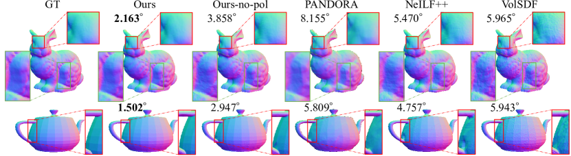
Figure 4: The reconstructed surface normal on the synthetic dataset. MAE metrics are on the top left. PANDORA [17] loses details of surface normals. NeILF++ [89], VolSDF [83], and ours-no-pol fail to disentangle the geometry and material. Thus, the estimated surface normals contain some patterns that come from the albedo.

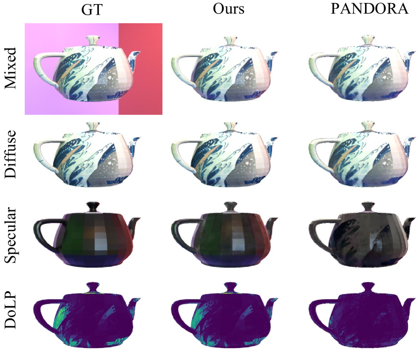
Figure 5: Diffuse-specular separation and DoLP images of synthetic dataset. We can observe the reflection of green and red walls on the teapot for our method, where PANDORA [17] fails.

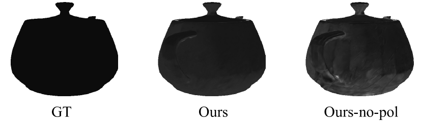
Figure 6: Roughness comparison. Without polarization cues, the recovered roughness is easily affected by geometry and shadows.

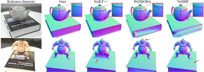
Figure 7: Qualitative comparison on real dataset. NeILF++ [89], PANDORA [17], and VolSDF [83] misinterpret materials as geometries. For example the flower pattern on the teapot and the text on the surface of the book. However, this is not correct because these patterns come from the albedo. On the other hand, our method can reconstruct a clean surface normal.

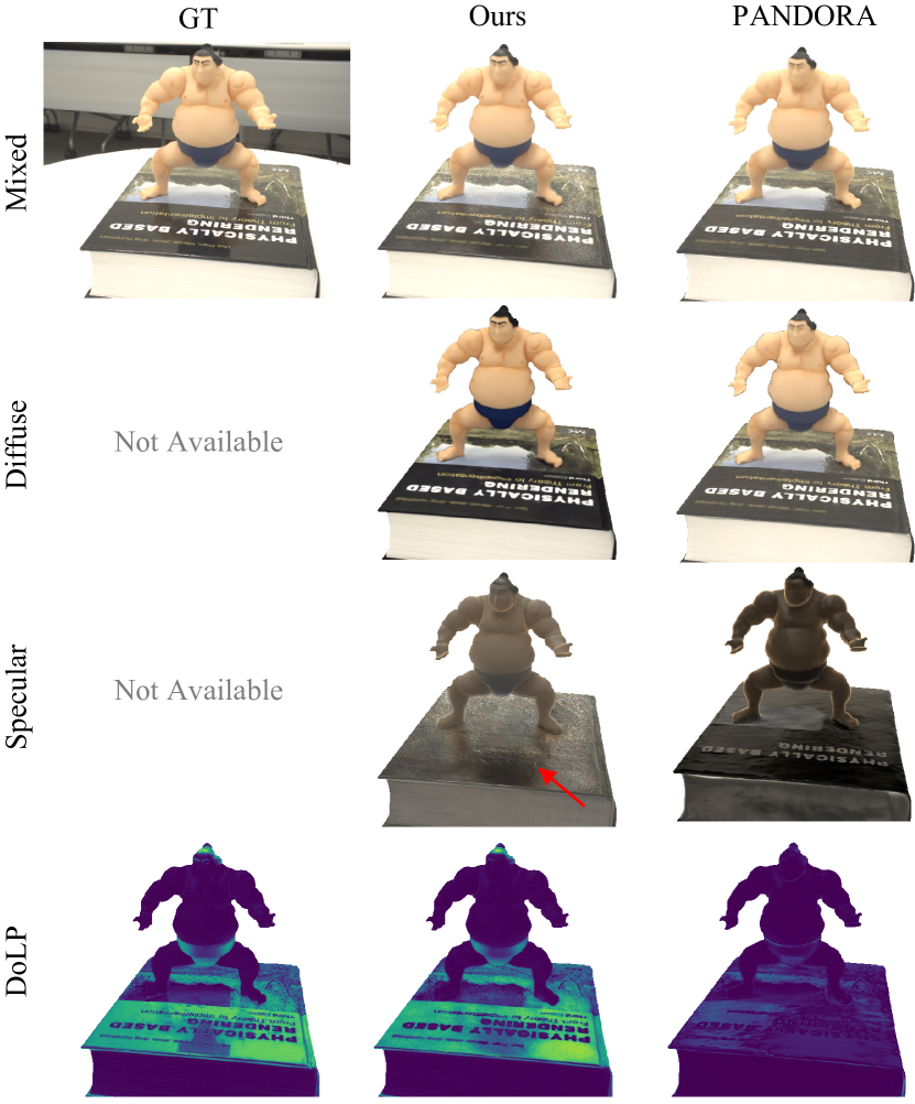
Figure 8: Diffuse-specular separation and DoLP images of real dataset. In the specular image, we can clearly observe the reflection on the surface of the book, but PANDORA [17] fails to reconstruct such kinds of results due to the single-bounce assumption. In addition, our DoLP is visually similar to the GT.

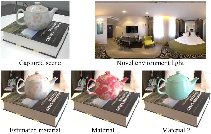
Figure 9: Relighting and material editing results. We edit the material of the teapot. Due to the accurate disentanglement of geometry and material, the edited image has realistic reflections.

5.2 Baselines

Looking for competitors for our proposal is not easy. Most of the NeRF-based inverse rendering works [7, 93, 60, 82, 89, 25, 29, 79, 15, 53] use Disney BRDF [12] model for rendering. Although they also estimate parameters such as roughness and albedo, these parameters have different physical meanings from ours, as Baek pBRDF is not based on Disney BRDF [12]. Nevertheless, the estimated surface normal as well as the reconstructed intensity images can be compared. Thus, we chose VolSDF [83] and the latest NeRF-based inverse rendering work NeILF++ [89] as our competitors. Because the official implementation of VolSDF does not support HDR images as inputs, we use our own implementation. Besides, PANDORA [17] is also considered as a baseline method. Although they do not support estimating BRDF parameters, the surface normal, diffuse-specular separation, and reconstructed polarized images are comparable. An important ablation study should be the performance with or without the presence of polarization cues. To achieve this, we introduce an unpolarized version of NeISF. Specifically, we remove $f_{\text{dif}}$ and $f_{\text{spec}}$ and only keep $f_{i}$. In addition, we also implement an unpolarized version of Beak pBRDF for rendering. Finally, the loss is only computed on the intensity space. The other parts are exactly the same as our model. We denote this model as Ours-no-pol, and it can also be considered as a variant of NeILF [82]. Details of this unpolarized BRDF can be found in the supplementary material.

5.3 Results

Synthetic Dataset We report the quantitative results of the surface normal, intensity, diffuse-specular separation, roughness, and albedo in Tab. 1. VolSDF does not support diffuse-specular separation. Although NeILF++ supports diffuse-specular separation, the diffuse and specular images differ from our physical meanings. Thus, we do not report diffuse-specular separation for these two methods. For the qualitative comparison, we show the surface normal results in Fig. 4, the diffuse-specular separation, and DoLP results in Fig. 5, and the roughness results in Fig. 6.

Real Dataset We show the surface normal results in Fig. 7, the diffuse-specular separation, and DoLP results in Fig. 8, and the material editing and relighting results in Fig. 9. Detailed analysis can be found in the figure captions.

6 Limitations

Several limitations still exist. First, the implicit Stokes representation is a double-edged sword. It allows us to model complicated polarimetric light transportation. At the same time, the estimated lighting can not be used in the conventional renderer. Second, the current solution only considers opaque dielectric objects. However, polarization cues can also provide rich information for translucent or metal objects. Finally, due to the manufacturing design of the polarization sensors, the captured four polarized images are not perfectly aligned. This makes the Stokes vectors of real-world data so noisy, making it impossible to handle high-frequency signals such as small bumps or edges.

7 Conclusion

We have proposed NeISF, an inverse rendering pipeline that combines implicit scene representations and polarization cues. It relies on the following novelties. The first one is an implicit representation of the multi-bounced Stokes vectors which takes care of the rotations. The second one is a physically-based polarimetric renderer. With these two novelties, NeISF outperforms the existing inverse render models for both synthetic and real-world datasets. The ablation study has verified the contribution of polarization cues. However, several limitations mentioned in Sec. 6 still exist and are worth further exploration.

References

- [1] Benjamin Attal, Eliot Laidlaw, Aaron Gokaslan, Changil Kim, Christian Richardt, James Tompkin, and Matthew O’Toole. Törf: Time-of-flight radiance fields for dynamic scene view synthesis. Advances in Neural Information Processing Systems, 34, 2021.
- [2] Dejan Azinović, Olivier Maury, Christophe Hery, Matthias Nießner, and Justus Thies. High-res facial appearance capture from polarized smartphone images. In Proceedings of the IEEE/CVF Conference on Computer Vision and Pattern Recognition, pages 16836–16846, 2023.
- [3] Yunhao Ba, Alex Gilbert, Franklin Wang, Jinfa Yang, Rui Chen, Yiqin Wang, Lei Yan, Boxin Shi, and Achuta Kadambi. Deep shape from polarization. In European Conference on Computer Vision, pages 554–571. Springer, 2020.
- [4] Seung-Hwan Baek and Felix Heide. All-photon polarimetric time-of-flight imaging. In Proceedings of the IEEE/CVF Conference on Computer Vision and Pattern Recognition, pages 17876–17885, 2022.
- [5] Seung-Hwan Baek, Daniel S Jeon, Xin Tong, and Min H Kim. Simultaneous acquisition of polarimetric svbrdf and normals. ACM Trans. Graph., 37(6):268–1, 2018.
- [6] Jonathan T Barron and Jitendra Malik. Shape, illumination, and reflectance from shading. IEEE transactions on pattern analysis and machine intelligence, 37(8):1670–1687, 2014.
- [7] Mark Boss, Raphael Braun, Varun Jampani, Jonathan T. Barron, Ce Liu, and Hendrik P.A. Lensch. Nerd: Neural reflectance decomposition from image collections. In IEEE International Conference on Computer Vision (ICCV), 2021.
- [8] Mark Boss, Andreas Engelhardt, Abhishek Kar, Yuanzhen Li, Deqing Sun, Jonathan T. Barron, Hendrik P.A. Lensch, and Varun Jampani. SAMURAI: Shape And Material from Unconstrained Real-world Arbitrary Image collections. In Advances in Neural Information Processing Systems (NeurIPS), 2022.
- [9] Mark Boss, Varun Jampani, Raphael Braun, Ce Liu, Jonathan T. Barron, and Hendrik P.A. Lensch. Neural-pil: Neural pre-integrated lighting for reflectance decomposition. In Advances in Neural Information Processing Systems (NeurIPS), 2021.
- [10] Mark Boss, Varun Jampani, Kihwan Kim, Hendrik Lensch, and Jan Kautz. Two-shot spatially-varying brdf and shape estimation. In Proceedings of the IEEE/CVF Conference on Computer Vision and Pattern Recognition, pages 3982–3991, 2020.
- [11] Mark Boss, Varun Jampani, Kihwan Kim, Hendrik P.A. Lensch, and Jan Kautz. Two-shot spatially-varying brdf and shape estimation. In IEEE Conference on Computer Vision and Pattern Recognition (CVPR), 2020.
- [12] Brent Burley and Walt Disney Animation Studios. Physically-based shading at disney. In Acm Siggraph, volume 2012, pages 1–7. vol. 2012, 2012.
- [13] Xu Cao, Hiroaki Santo, Fumio Okura, and Yasuyuki Matsushita. Multi-view azimuth stereo via tangent space consistency. In CVPR, 2023.
- [14] Guangcheng Chen, Li He, Yisheng Guan, and Hong Zhang. Perspective phase angle model for polarimetric 3d reconstruction. In Computer Vision–ECCV 2022: 17th European Conference, Tel Aviv, Israel, October 23–27, 2022, Proceedings, Part II, pages 398–414. Springer, 2022.
- [15] Ziang Cheng, Junxuan Li, and Hongdong Li. Wildlight: In-the-wild inverse rendering with a flashlight. In Proceedings of the IEEE/CVF Conference on Computer Vision and Pattern Recognition, pages 4305–4314, 2023.
- [16] Zhaopeng Cui, Viktor Larsson, and Marc Pollefeys. Polarimetric relative pose estimation. In Proceedings of the IEEE/CVF International Conference on Computer Vision, pages 2671–2680, 2019.
- [17] Akshat Dave, Yongyi Zhao, and Ashok Veeraraghavan. Pandora: Polarization-aided neural decomposition of radiance. In European Conference on Computer Vision, pages 538–556. Springer, 2022.
- [18] Valentin Deschaintre, Miika Aittala, Fredo Durand, George Drettakis, and Adrien Bousseau. Single-image svbrdf capture with a rendering-aware deep network. ACM Transactions on Graphics (ToG), 37(4):1–15, 2018.
- [19] Valentin Deschaintre, Yiming Lin, and Abhijeet Ghosh. Deep polarization imaging for 3d shape and svbrdf acquisition. In Proceedings of the IEEE/CVF Conference on Computer Vision and Pattern Recognition, pages 15567–15576, 2021.
- [20] Jin Duan, Youfei Hao, Ju Liu, Cai Cheng, Qiang Fu, and Huilin Jiang. End-to-end neural network for pbrdf estimation of object to reconstruct polarimetric reflectance. Optics Express, 31(24):39647–39663, 2023.
- [21] Yoshiki Fukao, Ryo Kawahara, Shohei Nobuhara, and Ko Nishino. Polarimetric normal stereo. In Proceedings of the IEEE/CVF Conference on Computer Vision and Pattern Recognition, pages 682–690, 2021.
- [22] Daoyi Gao, Yitong Li, Patrick Ruhkamp, Iuliia Skobleva, Magdalena Wysocki, HyunJun Jung, Pengyuan Wang, Arturo Guridi, and Benjamin Busam. Polarimetric pose prediction. In Computer Vision–ECCV 2022: 17th European Conference, Tel Aviv, Israel, October 23–27, 2022, Proceedings, Part IX, pages 735–752. Springer, 2022.
- [23] Saeed Hadadan, Shuhong Chen, and Matthias Zwicker. Neural radiosity. ACM Transactions on Graphics (TOG), 40(6):1–11, 2021.
- [24] Saeed Hadadan, Geng Lin, Jan Novák, Fabrice Rousselle, and Matthias Zwicker. Inverse global illumination using a neural radiometric prior. In ACM SIGGRAPH 2023 Conference Proceedings, pages 1–11, 2023.
- [25] Jon Hasselgren, Nikolai Hofmann, and Jacob Munkberg. Shape, light, and material decomposition from images using monte carlo rendering and denoising. Advances in Neural Information Processing Systems, 35:22856–22869, 2022.
- [26] Inseung Hwang, Daniel S Jeon, Adolfo Munoz, Diego Gutierrez, Xin Tong, and Min H Kim. Sparse ellipsometry: portable acquisition of polarimetric svbrdf and shape with unstructured flash photography. ACM Transactions on Graphics (TOG), 41(4):1–14, 2022.
- [27] Tomoki Ichikawa, Matthew Purri, Ryo Kawahara, Shohei Nobuhara, Kristin Dana, and Ko Nishino. Shape from sky: Polarimetric normal recovery under the sky. In Proceedings of the IEEE/CVF Conference on Computer Vision and Pattern Recognition, pages 14832–14841, 2021.
- [28] Wenzel Jakob, Sébastien Speierer, Nicolas Roussel, and Delio Vicini. Dr.jit: A just-in-time compiler for differentiable rendering. Transactions on Graphics (Proceedings of SIGGRAPH), 41(4), July 2022.
- [29] Haian Jin, Isabella Liu, Peijia Xu, Xiaoshuai Zhang, Songfang Han, Sai Bi, Xiaowei Zhou, Zexiang Xu, and Hao Su. Tensoir: Tensorial inverse rendering. In Proceedings of the IEEE/CVF Conference on Computer Vision and Pattern Recognition, pages 165–174, 2023.
- [30] Achuta Kadambi, Vage Taamazyan, Boxin Shi, and Ramesh Raskar. Polarized 3d: High-quality depth sensing with polarization cues. In Proceedings of the IEEE International Conference on Computer Vision, pages 3370–3378, 2015.
- [31] James T Kajiya. The rendering equation. In Proceedings of the 13th annual conference on Computer graphics and interactive techniques, pages 143–150, 1986.
- [32] Agastya Kalra, Vage Taamazyan, Supreeth Krishna Rao, Kartik Venkataraman, Ramesh Raskar, and Achuta Kadambi. Deep polarization cues for transparent object segmentation. In Proceedings of the IEEE/CVF Conference on Computer Vision and Pattern Recognition, pages 8602–8611, 2020.
- [33] Kichang Kim, Akihiko Torii, and Masatoshi Okutomi. Multi-view inverse rendering under arbitrary illumination and albedo. In Computer Vision–ECCV 2016: 14th European Conference, Amsterdam, The Netherlands, October 11-14, 2016, Proceedings, Part III 14, pages 750–767. Springer, 2016.
- [34] Youngchan Kim, Wonjoon Jin, Sunghyun Cho, and Seung-Hwan Baek. Neural spectro-polarimetric fields. arXiv preprint arXiv:2306.12562, 2023.
- [35] Yuhi Kondo, Taishi Ono, Legong Sun, Yasutaka Hirasawa, and Jun Murayama. Accurate polarimetric brdf for real polarization scene rendering. In European Conference on Computer Vision, pages 220–236. Springer, 2020.
- [36] Hyun Jin Ku, Hyunho Hat, Joo Ho Lee, Dahyun Kang, James Tompkin, and Min H Kim. Differentiable appearance acquisition from a flash/no-flash rgb-d pair. In 2022 IEEE International Conference on Computational Photography (ICCP), pages 1–12. IEEE, 2022.
- [37] Teppei Kurita, Yuhi Kondo, Legong Sun, and Yusuke Moriuchi. Simultaneous acquisition of high quality rgb image and polarization information using a sparse polarization sensor. In Proceedings of the IEEE/CVF Winter Conference on Applications of Computer Vision, pages 178–188, 2023.
- [38] Chenyang Lei, Xuhua Huang, Mengdi Zhang, Qiong Yan, Wenxiu Sun, and Qifeng Chen. Polarized reflection removal with perfect alignment in the wild. In Proceedings of the IEEE/CVF Conference on Computer Vision and Pattern Recognition, pages 1750–1758, 2020.
- [39] Chenyang Lei, Chenyang Qi, Jiaxin Xie, Na Fan, Vladlen Koltun, and Qifeng Chen. Shape from polarization for complex scenes in the wild. In Proceedings of the IEEE/CVF Conference on Computer Vision and Pattern Recognition, pages 12632–12641, 2022.
- [40] Chunyu Li, Yusuke Monno, and Masatoshi Okutomi. Spectral mvir: Joint reconstruction of 3d shape and spectral reflectance. In 2021 IEEE International Conference on Computational Photography (ICCP), pages 1–12. IEEE, 2021.
- [41] Chenhao Li, Trung Thanh Ngo, and Hajime Nagahara. Inverse rendering of translucent objects using physical and neural renderers. In Proceedings of the IEEE/CVF Conference on Computer Vision and Pattern Recognition, pages 12510–12520, 2023.
- [42] Junxuan Li and Hongdong Li. Neural reflectance for shape recovery with shadow handling. In Proceedings of the IEEE/CVF Conference on Computer Vision and Pattern Recognition, pages 16221–16230, 2022.
- [43] Rui Li, Simeng Qiu, Guangming Zang, and Wolfgang Heidrich. Reflection separation via multi-bounce polarization state tracing. In Computer Vision–ECCV 2020: 16th European Conference, Glasgow, UK, August 23–28, 2020, Proceedings, Part XIII 16, pages 781–796. Springer, 2020.
- [44] Tzu-Mao Li, Miika Aittala, Frédo Durand, and Jaakko Lehtinen. Differentiable monte carlo ray tracing through edge sampling. ACM Transactions on Graphics (TOG), 37(6):1–11, 2018.
- [45] Zhengqin Li, Mohammad Shafiei, Ravi Ramamoorthi, Kalyan Sunkavalli, and Manmohan Chandraker. Inverse rendering for complex indoor scenes: Shape, spatially-varying lighting and svbrdf from a single image. In Proceedings of the IEEE/CVF Conference on Computer Vision and Pattern Recognition, pages 2475–2484, 2020.
- [46] Zhengqin Li, Kalyan Sunkavalli, and Manmohan Chandraker. Materials for masses: Svbrdf acquisition with a single mobile phone image. In Proceedings of the European Conference on Computer Vision (ECCV), pages 72–87, 2018.
- [47] Zhen Li, Lingli Wang, Mofang Cheng, Cihui Pan, and Jiaqi Yang. Multi-view inverse rendering for large-scale real-world indoor scenes. In Proceedings of the IEEE/CVF Conference on Computer Vision and Pattern Recognition, pages 12499–12509, 2023.
- [48] Zhen Li, Lingli Wang, Xiang Huang, Cihui Pan, and Jiaqi Yang. Phyir: Physics-based inverse rendering for panoramic indoor images. In Proceedings of the IEEE/CVF Conference on Computer Vision and Pattern Recognition, pages 12713–12723, 2022.
- [49] Zhengqin Li, Zexiang Xu, Ravi Ramamoorthi, Kalyan Sunkavalli, and Manmohan Chandraker. Learning to reconstruct shape and spatially-varying reflectance from a single image. ACM Transactions on Graphics (TOG), 37(6):1–11, 2018.
- [50] Yupeng Liang, Ryosuke Wakaki, Shohei Nobuhara, and Ko Nishino. Multimodal material segmentation. In Proceedings of the IEEE/CVF Conference on Computer Vision and Pattern Recognition, pages 19800–19808, 2022.
- [51] Daniel Lichy, Jiaye Wu, Soumyadip Sengupta, and David W Jacobs. Shape and material capture at home. In Proceedings of the IEEE/CVF Conference on Computer Vision and Pattern Recognition, pages 6123–6133, 2021.
- [52] Jingwang Ling, Zhibo Wang, and Feng Xu. Shadowneus: Neural sdf reconstruction by shadow ray supervision. In Proceedings of the IEEE/CVF Conference on Computer Vision and Pattern Recognition, pages 175–185, 2023.
- [53] Yuan Liu, Peng Wang, Cheng Lin, Xiaoxiao Long, Jiepeng Wang, Lingjie Liu, Taku Komura, and Wenping Wang. Nero: Neural geometry and brdf reconstruction of reflective objects from multiview images. arXiv preprint arXiv:2305.17398, 2023.
- [54] Stephen Lombardi and Ko Nishino. Reflectance and illumination recovery in the wild. IEEE transactions on pattern analysis and machine intelligence, 38(1):129–141, 2015.
- [55] Stephen Lombardi and Ko Nishino. Radiometric scene decomposition: Scene reflectance, illumination, and geometry from rgb-d images. In 2016 fourth international conference on 3d vision (3dv), pages 305–313. IEEE, 2016.
- [56] Youwei Lyu, Zhaopeng Cui, Si Li, Marc Pollefeys, and Boxin Shi. Reflection separation using a pair of unpolarized and polarized images. Advances in neural information processing systems, 32, 2019.
- [57] Haiyang Mei, Bo Dong, Wen Dong, Jiaxi Yang, Seung-Hwan Baek, Felix Heide, Pieter Peers, Xiaopeng Wei, and Xin Yang. Glass segmentation using intensity and spectral polarization cues. In Proceedings of the IEEE/CVF Conference on Computer Vision and Pattern Recognition, pages 12622–12631, 2022.
- [58] Ben Mildenhall, Pratul P Srinivasan, Matthew Tancik, Jonathan T Barron, Ravi Ramamoorthi, and Ren Ng. Nerf: Representing scenes as neural radiance fields for view synthesis. In European Conference on Computer Vision, pages 405–421. Springer, 2020.
- [59] Yasuhiro Mukaigawa, Yasushi Yagi, and Ramesh Raskar. Analysis of light transport in scattering media. In 2010 IEEE Computer Society Conference on Computer Vision and Pattern Recognition, pages 153–160. IEEE, 2010.
- [60] Jacob Munkberg, Jon Hasselgren, Tianchang Shen, Jun Gao, Wenzheng Chen, Alex Evans, Thomas Müller, and Sanja Fidler. Extracting triangular 3d models, materials, and lighting from images. In Proceedings of the IEEE/CVF Conference on Computer Vision and Pattern Recognition, pages 8280–8290, 2022.
- [61] Trung Ngo Thanh, Hajime Nagahara, and Rin-ichiro Taniguchi. Shape and light directions from shading and polarization. In Proceedings of the IEEE conference on computer vision and pattern recognition, pages 2310–2318, 2015.
- [62] Baptiste Nicolet, Fabrice Rousselle, Jan Novak, Alexander Keller, Wenzel Jakob, and Thomas Müller. Recursive control variates for inverse rendering. ACM Transactions on Graphics (TOG), 42(4):1–13, 2023.
- [63] Merlin Nimier-David, Delio Vicini, Tizian Zeltner, and Wenzel Jakob. Mitsuba 2: A retargetable forward and inverse renderer. ACM Transactions on Graphics (TOG), 38(6):1–17, 2019.
- [64] Ko Nishino. Directional statistics brdf model. In 2009 IEEE 12th International Conference on Computer Vision, pages 476–483. IEEE, 2009.
- [65] Taishi Ono, Yuhi Kondo, Legong Sun, Teppei Kurita, and Yusuke Moriuchi. Degree-of-linear-polarization-based color constancy. In Proceedings of the IEEE/CVF Conference on Computer Vision and Pattern Recognition, pages 19740–19749, 2022.
- [66] Geoffrey Oxholm and Ko Nishino. Multiview shape and reflectance from natural illumination. In Proceedings of the IEEE Conference on Computer Vision and Pattern Recognition, pages 2155–2162, 2014.
- [67] Henry Peters, Yunhao Ba, and Achuta Kadambi. pcon: Polarimetric coordinate networks for neural scene representations. In Proceedings of the IEEE/CVF Conference on Computer Vision and Pattern Recognition, pages 16579–16589, 2023.
- [68] Matteo Poggi, Pierluigi Zama Ramirez, Fabio Tosi, Samuele Salti, Luigi Di Stefano, and Stefano Mattoccia. Cross-spectral neural radiance fields. In Proceedings of the International Conference on 3D Vision, 2022. 3DV.
- [69] Shen Sang and Manmohan Chandraker. Single-shot neural relighting and svbrdf estimation. In European Conference on Computer Vision, pages 85–101. Springer, 2020.
- [70] Soumyadip Sengupta, Jinwei Gu, Kihwan Kim, Guilin Liu, David W Jacobs, and Jan Kautz. Neural inverse rendering of an indoor scene from a single image. In Proceedings of the IEEE/CVF International Conference on Computer Vision, pages 8598–8607, 2019.
- [71] Soumyadip Sengupta, Angjoo Kanazawa, Carlos D Castillo, and David W Jacobs. Sfsnet: Learning shape, reflectance and illuminance of facesin the wild’. In Proceedings of the IEEE conference on computer vision and pattern recognition, pages 6296–6305, 2018.
- [72] Mingqi Shao, Chongkun Xia, Zhendong Yang, Junnan Huang, and Xueqian Wang. Transparent shape from a single view polarization image. arXiv preprint arXiv:2204.06331, 2022.
- [73] Pratul P Srinivasan, Boyang Deng, Xiuming Zhang, Matthew Tancik, Ben Mildenhall, and Jonathan T Barron. Nerv: Neural reflectance and visibility fields for relighting and view synthesis. In Proceedings of the IEEE/CVF Conference on Computer Vision and Pattern Recognition, pages 7495–7504, 2021.
- [74] Kushagra Tiwary, Akshat Dave, Nikhil Behari, Tzofi Klinghoffer, Ashok Veeraraghavan, and Ramesh Raskar. Orca: Glossy objects as radiance-field cameras. In Proceedings of the IEEE/CVF Conference on Computer Vision and Pattern Recognition, pages 20773–20782, 2023.
- [75] Bruce Walter, Stephen R Marschner, Hongsong Li, and Kenneth E Torrance. Microfacet models for refraction through rough surfaces. In Proceedings of the 18th Eurographics conference on Rendering Techniques, pages 195–206, 2007.
- [76] Peng Wang, Lingjie Liu, Yuan Liu, Christian Theobalt, Taku Komura, and Wenping Wang. Neus: Learning neural implicit surfaces by volume rendering for multi-view reconstruction. Advances in Neural Information Processing Systems, 34:27171–27183, 2021.
- [77] Zian Wang, Jonah Philion, Sanja Fidler, and Jan Kautz. Learning indoor inverse rendering with 3d spatially-varying lighting. In Proceedings of the IEEE/CVF International Conference on Computer Vision (ICCV), pages 12538–12547, October 2021.
- [78] Zian Wang, Tianchang Shen, Jun Gao, Shengyu Huang, Jacob Munkberg, Jon Hasselgren, Zan Gojcic, Wenzheng Chen, and Sanja Fidler. Neural fields meet explicit geometric representations for inverse rendering of urban scenes. In Proceedings of the IEEE/CVF Conference on Computer Vision and Pattern Recognition, pages 8370–8380, 2023.
- [79] Haoqian Wu, Zhipeng Hu, Lincheng Li, Yongqiang Zhang, Changjie Fan, and Xin Yu. Nefii: Inverse rendering for reflectance decomposition with near-field indirect illumination. In Proceedings of the IEEE/CVF Conference on Computer Vision and Pattern Recognition, pages 4295–4304, 2023.
- [80] Tomohiro Yamazaki, Yasushi Maruyama, Yusuke Uesaka, Motoaki Nakamura, Yoshihisa Matoba, Takashi Terada, Kenta Komori, Yoshiyuki Ohba, Shinichi Arakawa, Yasutaka Hirasawa, et al. Four-directional pixel-wise polarization cmos image sensor using air-gap wire grid on 2.5-m back-illuminated pixels. In 2016 IEEE International Electron Devices Meeting (IEDM), pages 8–7. IEEE, 2016.
- [81] Wenqi Yang, Guanying Chen, Chaofeng Chen, Zhenfang Chen, and Kwan-Yee K. Wong. S3-nerf: Neural reflectance field from shading and shadow under a single viewpoint. In Conference on Neural Information Processing Systems (NeurIPS), 2022.
- [82] Yao Yao, Jingyang Zhang, Jingbo Liu, Yihang Qu, Tian Fang, David McKinnon, Yanghai Tsin, and Long Quan. Neilf: Neural incident light field for physically-based material estimation. In European Conference on Computer Vision, pages 700–716. Springer, 2022.
- [83] Lior Yariv, Jiatao Gu, Yoni Kasten, and Yaron Lipman. Volume rendering of neural implicit surfaces. Advances in Neural Information Processing Systems, 34:4805–4815, 2021.
- [84] Lior Yariv, Peter Hedman, Christian Reiser, Dor Verbin, Pratul P. Srinivasan, Richard Szeliski, Jonathan T. Barron, and Ben Mildenhall. Bakedsdf: Meshing neural sdfs for real-time view synthesis. arXiv, 2023.
- [85] Lior Yariv, Yoni Kasten, Dror Moran, Meirav Galun, Matan Atzmon, Basri Ronen, and Yaron Lipman. Multiview neural surface reconstruction by disentangling geometry and appearance. Advances in Neural Information Processing Systems, 33:2492–2502, 2020.
- [86] Kuk-Jin Yoon, Emmanuel Prados, and Peter Sturm. Joint estimation of shape and reflectance using multiple images with known illumination conditions. International Journal of Computer Vision, 86(2-3):192–210, 2010.
- [87] Cheng Zhang, Bailey Miller, Kai Yan, Ioannis Gkioulekas, and Shuang Zhao. Path-space differentiable rendering. ACM Trans. Graph., 39(4):143:1–143:19, 2020.
- [88] Cheng Zhang, Lifan Wu, Changxi Zheng, Ioannis Gkioulekas, Ravi Ramamoorthi, and Shuang Zhao. A differential theory of radiative transfer. ACM Trans. Graph., 38(6):227:1–227:16, 2019.
- [89] Jingyang Zhang, Yao Yao, Shiwei Li, Jingbo Liu, Tian Fang, David McKinnon, Yanghai Tsin, and Long Quan. Neilf++: Inter-reflectable light fields for geometry and material estimation. arXiv preprint arXiv:2303.17147, 2023.
- [90] Kai Zhang, Fujun Luan, Zhengqi Li, and Noah Snavely. Iron: Inverse rendering by optimizing neural sdfs and materials from photometric images. In Proceedings of the IEEE/CVF Conference on Computer Vision and Pattern Recognition, pages 5565–5574, 2022.
- [91] Kai Zhang, Fujun Luan, Qianqian Wang, Kavita Bala, and Noah Snavely. Physg: Inverse rendering with spherical gaussians for physics-based material editing and relighting. In Proceedings of the IEEE/CVF Conference on Computer Vision and Pattern Recognition, pages 5453–5462, 2021.
- [92] Xiuming Zhang, Pratul P Srinivasan, Boyang Deng, Paul Debevec, William T Freeman, and Jonathan T Barron. Nerfactor: Neural factorization of shape and reflectance under an unknown illumination. ACM Transactions on Graphics (ToG), 40(6):1–18, 2021.
- [93] Yuanqing Zhang, Jiaming Sun, Xingyi He, Huan Fu, Rongfei Jia, and Xiaowei Zhou. Modeling indirect illumination for inverse rendering. In Proceedings of the IEEE/CVF Conference on Computer Vision and Pattern Recognition, pages 18643–18652, 2022.
- [94] Jinyu Zhao, Yusuke Monno, and Masatoshi Okutomi. Polarimetric multi-view inverse rendering. IEEE Transactions on Pattern Analysis and Machine Intelligence, 2022.
- [95] Jingsen Zhu, Yuchi Huo, Qi Ye, Fujun Luan, Jifan Li, Dianbing Xi, Lisha Wang, Rui Tang, Wei Hua, Hujun Bao, et al. I2-sdf: Intrinsic indoor scene reconstruction and editing via raytracing in neural sdfs. In Proceedings of the IEEE/CVF Conference on Computer Vision and Pattern Recognition, pages 12489–12498, 2023.
- [96] Rui Zhu, Zhengqin Li, Janarbek Matai, Fatih Porikli, and Manmohan Chandraker. Irisformer: Dense vision transformers for single-image inverse rendering in indoor scenes. In Proceedings of the IEEE/CVF Conference on Computer Vision and Pattern Recognition, pages 2822–2831, 2022.
- [97] Shihao Zou, Xinxin Zuo, Yiming Qian, Sen Wang, Chi Xu, Minglun Gong, and Li Cheng. 3d human shape reconstruction from a polarization image. In European Conference on Computer Vision, pages 351–368. Springer, 2020.
- [98] Shihao Zou, Xinxin Zuo, Sen Wang, Yiming Qian, Chuan Guo, and Li Cheng. Human pose and shape estimation from single polarization images. IEEE Transactions on Multimedia, 2022.