Applications of Spiking Neural Networks in Visual Place Recognition

Abstract

In robotics, Spiking Neural Networks (SNNs) are increasingly recognized for their largely-unrealized potential energy efficiency and low latency particularly when implemented on neuromorphic hardware. Our paper highlights three advancements for SNNs in Visual Place Recognition (VPR). First, we propose Modular SNNs, where each SNN represents a set of non-overlapping geographically distinct places, enabling scalable networks for large environments. Secondly, we present Ensembles of Modular SNNs, where multiple networks represent the same place, significantly enhancing accuracy compared to single-network models. Our SNNs are compact and small, comprising only 1500 neurons and 474k synapses, which makes them ideally suited for ensembling due to this small size. Lastly, we investigate the role of sequence matching in SNN-based VPR, a technique where consecutive images are used to refine place recognition. We analyze the responsiveness of SNNs to ensembling and sequence matching compared to other VPR techniques. Our contributions highlight the viability of SNNs for VPR, offering scalable and robust solutions, paving the way for their application in various energy-sensitive robotic tasks.

I Introduction

Spiking Neural Networks (SNNs) represent a cutting-edge paradigm in neuromorphic computing, mirroring the intricate workings of biological neural systems [1, 2, 3, 4]. In these networks, every neuron possesses its distinct activation state. Unlike conventional neural networks, where neuron activations are typically continuous values, neurons in SNNs convey information through intermittent spikes, which are initiated when the neuron’s activation surpasses a particular threshold [1, 5, 6]. These spiking networks exhibit promising attributes when deployed on neuromorphic hardware, offering notable energy efficiency and low-latency data processing [7, 8, 2, 9, 10]. Despite these potential advantages, SNNs have seen minimal adaptation in robotics, due to limitations such as difficulty in supervised training of SNNs due to the non-differentiable activation function of spiking neurons and a lack of tools and resources [2, 11, 6, 12, 4].

One robotics application that could benefit substantially from the emerging neuromorphic computing paradigm is the Visual Place Recognition (VPR) task, a vital process in robotic navigation. At its core, the objective is seemingly straightforward: given a query image of a place, find the corresponding place out of a potentially very large list of previously visited places, also called the reference dataset [13, 14, 15, 16, 17, 18]. Yet there are immense underlying challenges such as changes in appearance due to different times of the day, variations in seasons, weather conditions, and perceptual aliasing (where two geographically distant places may look very similar) which can significantly change the appearance of the query image [14, 15, 17]. Visual place recognition is a critical component in robot localization tasks such as loop closure detection in SLAM, and global re-localization of mobile robots [19, 13, 18, 16].

The objective of our work is to explore an alternative SNN-based approach to current state-of-the-art VPR techniques based on deep learning that is scalable and efficient, and has the prospect to be ideally suited for energy-sensitive robotic tasks. We achieve this by demonstrating the potential of a simple three-layer SNN in achieving place recognition at a significant scale. Our approach leverages widely adopted strategies for enhancing the robustness of conventional machine learning approaches, specifically focusing on modularity, ensembling, and sequence matching techniques. The subsequent paragraphs will offer a succinct overview of these key strategies.

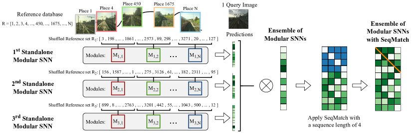
Figure 1: Schematic of the proposed algorithm: The basic building blocks in our work are independent Spiking Neural Network (SNN) modules that learn small subsets of the reference database. At inference time, the place predictions of all these modules are fused in parallel in what we dub a “Standalone Modular SNN”. We further make use of the potential massively parallel processing capabilities of neuromorphic processors by introducing ensembles in which multiple Modular SNNs learn representations for the same place, and demonstrate that SNNs are more responsive to ensembling compared to conventional techniques. Finally, we demonstrate high responsiveness of these Ensembles of Modular SNNs to sequence matching.

Modularity, a prominent concept in machine learning, entails the design of systems comprising distinct modules, each dedicated to a specific task [20, 21, 22]. These modules can be combined to form more intricate systems, offering scalability benefits beyond what individual modules can achieve [20, 21, 22]. Modularity has been employed in [23] for a SLAM system with heterogeneous sensor configuration, a 3D place recognition task [24], a condition and environment-invariant place recognition task [25], and a SLAM system [26]. These works assign a module to each structurally different sub-task of a system. In our work, we similarly use the concept of modularity to enable robustness to more challenging scenarios, however we create modules with the same architecture which are assigned to learn small segments of the dataset.

Ensembling is the strategy of combining multiple models to boost accuracy, reduce overfitting, and yield more robust models [1, 27, 29, 30, 31, 32]. While there is an inherent trade-off between the number of ensemble members and the energy efficiency of a system [27, 29], the benefits of ensembling, particularly its enhanced accuracy and reliability, are invaluable to navigation-related robotics applications, where it was previously utilized in the context of monocular SLAM [33] for improved data association, terrain segmentation for learning the seen data that is collected at different points of time [34], and place recognition with image-based [35, 36] and event-based [37] input, where the prediction of multiple VPR techniques are fused to improve place recognition robustness. Similarly, our work also utilizes ensembling to improve upon the robustness and generalization ability of our system but differs with these works in terms of how we define our ensemble members. Our ensemble members all are tasked to do the same task, have the same architecture and differ in random shuffling of input images and initial learned weights. A similar approach of employing ensembles was previously demonstrated in uncertainty estimation to provide sufficient diversity among the members, and improve the overall performance of the system [38].

In the context of VPR, a sequence matching technique uses consecutive reference frames instead of single frames, to match a query image of a place to its corresponding reference image [39, 40, 41]. By analyzing a series of images, this technique enables enhanced resilience against temporary environmental disruptions and improves localization accuracy [39, 40, 41]. Sequence matching techniques have been widely employed in place recognition [39, 42, 41, 43, 40, 44, 45], where often a decoupled approach consisting of an initial image-based retrieval method and subsequent sequence score aggregation [39, 42, 45] is employed. Similar to these techniques, our paper utilizes sequence matching as an additional step after image retrieval. We further demonstrate the effectiveness of sequence matching for SNN-based approaches, and provide an indicator for responsiveness of conventional and SNN-based VPR methods to sequence matching.

In this work, we claim the following contributions (Figure 1):

1. We present the concept of modular spiking neural networks (Modular SNNs) for scalable place recognition. Each module of the network specializes in a small subset of places in the environment at training time and operates independently of all other networks. After training the modules independently, we address the lack of global regularization by detecting hyperactive neurons, those that frequently respond to images outside their training data, and subsequently ignoring them during deployment. The query image at inference time is provided to all modules in parallel, and their place predictions are fused.

2. While the first contribution serves as a functional framework for scalable place recognition with Modular SNNs, this second contribution further enhances its capabilities through Ensembles of Modular SNNs, where multiple networks learn a representation for the same place, leading to improved robustness and generalization capabilities. Each ensemble member constitutes a Modular SNN with variations in the weight initialization and the set of distinct places learned by a module. Our results demonstrate that SNN ensemble members exhibit higher variations in their match predictions compared to conventional counterparts, which results in significantly higher responsiveness to ensembling.

3. We analyze the responsiveness of our Modular and Ensemble of Modular SNNs to sequence matching which captures the temporal information inherent in the data by considering multiple consecutive reference places for predicting a single query image as opposed to considering one single reference image. We also present an indicator that predicts the effectiveness of applying sequence matching to both conventional VPR methods and our spiking networks to provide insights into the improvements conferred by applying a sequence matching technique.

4. We provide extensive evaluations of our SNN performance, and compare them to conventional VPR techniques, i.e. Sum-of-absolute differences (SAD) [39], NetVLAD [46], DenseVLAD[47], AP-GeM [48], and GCL [49] across multiple benchmark datasets, namely Nordland [50], Oxford RobotCar [51], SFU-Mountain [52], Synthia Night to Fall [53], and St Lucia [54]. We also introspect our SNNs and provide insights to their responsiveness when paired with sequence matching, and contrast that to that of conventional VPR techniques.

The first contribution on Modular SNNs was previously presented at the IEEE International Conference on Robotics and Automation (ICRA) 2023 [55]. This work substantially extends on [55] by employing ensembling and sequence matching techniques to significantly enhance place recognition capabilities and analyzing the impact of these techniques across the entire set of evaluated models. We introduce an indicator that predicts the responsiveness of both conventional VPR techniques and our spiking networks to sequence matching. We also provide significantly extended evaluations, now covering six datasets, up from the initial two. We also benchmark against five distinct VPR techniques, encompassing 12 variations, compared to the three techniques previously compared against in [55]. Our new contributions demonstrate the enhanced effectiveness of SNNs for VPR, including increased scalability and robustness, paving the way for application in energy-efficient robotic navigation tasks.

In the following sections, we will delve into the related works (Section II) to provide context for spiking neural networks and visual place recognition, discuss our methodology (Section III), and experimental setup (Section IV), present our results with analysis (Section V), and propose future research directions (Section VI), offering a thorough exploration of spiking neural networks for scalable visual place recognition.

II Related works

In this section, we offer an overview of neuromorphic computing and spiking neural networks (Section II-A) and explore the applications of spiking neural networks (SNNs) in robot localization (Section II-B). We then delve into the visual place recognition task (Section II-C), non-spiking biologically inspired VPR approaches (Section II-D) and provide insights into ensembling (Section II-E) and sequence matching techniques (Section II-F).

II-A Neuromorphic Computing and Spiking Neural Networks

The field of neuromorphic computing focuses on hardware, sensors, and algorithms inspired by biological neural networks, aiming to capture the robustness, generalization capability, energy efficiency and low latency advantages seen in nature [2, 8, 7]. The fundamental properties of neuromorphic computing that enable its advantageous features encompass highly parallel operations, the integration of processor and memory components, and the utilization of event-driven computation with sparse temporal activity [3, 2, 8].

SNNs represent a set of algorithms within the realm of neuromorphic computing. Various common approaches exist for implementing SNNs. One common approach to develop SNNs is to train an Artificial Neural Network (ANN) using back-propagation and perform a conversion process to map the trained model to an SNN for inference. Strategies for this conversion include activation function approximations [56], and optimizations [57, 58], constrained training to resemble spiking form [59, 60], and optimized spiking neuron model [61]. However, due to limited weight precision, these approaches often have reduced performance compared to their ANN counterparts when deployed on neuromorphic hardware. They often also do not fully utilize the inherent computational capabilities of SNNs in terms of high energy efficiency [3].

The neuronal dynamics of spiking neurons are non-differentiable. This characteristic means that well-established learning techniques used in deep learning such as back-propagation cannot be directly transferred to train SNNs for complex tasks. To address this issue, a number of works have focused on approximating back-propagation for SNNs [62, 63, 64]. However, these methods require offline training with large amount of data and do not perform well in continual learning settings due to catastrophic forgetting [2].

Lastly, some training paradigms are inspired by the modulation of synaptic strength (weight) based on the activity of interconnected neurons [65]. Among these, Spike-Time Dependent Plasticity (STDP) updates weights according to the relative timing of spikes received from presynaptic and postsynaptic neurons in the connection [65, 3]. Leveraging biologically inspired unsupervised learning algorithms is highly promising for fully harnessing the advantages of computational SNNs including optimized latencies and energy efficiency [8], however the accuracy of these unsupervised approaches is often not competitive.

II-B Spiking Neural Networks for Robot Localization

The capabilities of SNNs have been demonstrated in a wide range of computer vision and robotics tasks. These include pattern recognition [66], control [67, 68, 69, 70, 71], manipulation [72, 73, 74], object tracking [75, 76], and scene understanding [77, 78]. Many works have used SNNs to address the robot localization task which is the problem being investigated in this work. These works include RatSLAM [79] which computationally models place, grid and border cells of the rat hippocampus[80], a navigation controller for mapping unknown environments [81], a pose estimation and map formation method [82], a light-weight system for uni-dimensional SLAM [83], and a SLAM model that utilizes representations of continuous spatial maps to produce compressed structures from multiple domains [84]. In previous work [85], we presented a SNN specifically for VPR. This network had a limited capacity, recognizing up to just 100 places.

While some of these systems have also been deployed on neuromorphic hardware [80, 82, 83, 86, 87], so far, the performance of SNN-based methods for robot localization have only been demonstrated in simulated environments [81, 82, 84], constrained indoor environments [80, 83, 86, 87, 88], or small-scale outdoor environments [85].

In addition to spike-based processing, the use of event-based cameras for spike-based sensing has shown promising advantages in robotic navigation systems [89, 90, 91], SLAM systems [86, 87, 88], and place recognition [92], owing to their unique ability to output asynchronous pixel-level brightness changes rather than conventional images, having a high dynamic range and remaining unaffected by motion blur [93].

II-C Visual Place Recognition

The visual place recognition (VPR) task is to determine whether a place has been previously visited, even when faced with appearance changes and perceptual aliasing [15, 17, 18, 14, 13]. The VPR problem is typically posed as a template matching problem where associated templates of all reference images are extracted to represent each place either via a single image [94, 46, 95, 47] or a sequence of images [39, 40, 96].

Learning-based approaches are dominating in VPR. Notably, NetVLAD [46], a method based on Vector of Locally Aggregated Descriptors (VLAD) [97], has been influential in producing robust feature representations. Recent advances partitioned training datasets into smaller segments, similar to our approach, and employed an ensemble of classifiers for each segment, facilitating large-scale VPR. For instance, the ‘Divide and Classify’ method [98] divides the reference dataset into non-overlapping classes. Each segment is processed by an individual classifier, and the collective ensemble is employed for predictions, enabling fast inference for large-scale VPR. On the other hand, Cosplace [99] reimagines the training process, viewing it as a classification task and sidestepping the resource-intensive process of mining positive and negative samples inherent in contrastive learning. Notably, both these works [98, 99] and ours share a common thread: framing VPR as a classification task to further scale place recognition capabilities.

We now review hierarchical approaches to demonstrate the broader landscape of methods aimed at improving recognition accuracy and robustness in VPR, providing a foundation for our exploration of ensembling techniques. Hierarchical techniques have been previously used for coarse-to-fine refinement frameworks via a monolithic neural network to efficiently predict hierarchical features (HF-Net) [100], probabilistic approaches [94], bio-inspired approaches [101], multi-process fusion [102], global-to-local VPR pipeline to guide local feature matching via global descriptors [103], and hierarchical decomposition of the environment [104]. In the latter approach, places with similar visual features are grouped together in nodes to reduce search space while maintaining high accuracy [104].

II-D Non-spiking Biologically Inspired VPR Approaches

Biologically inspired VPR methods seek to emulate the navigational capabilities of animals with relatively small brains such as ants, bees, and rodents [79, 101, 105, 106, 107, 108] to design energy-efficient and high-performing solutions. These non-spiking biologically inspired techniques offer valuable reference points for our spike-based work.

The place cells and head direction cells in rodent hippocampus inspired RatSLAM [79]. RatSLAM was later extended to include grid cells in [101] and extended to 3D in NeuroSLAM [106]. Inspired by the principles of Hierarchical Temporal Memory related to the human neocortex, [105] details a minicolumn network to pool spatial information and preserve temporal memory. [107] combines a pattern recognition module, inspired by fruit flies olfactory neural circuit, with a one-dimensional continuous attractor network serving as the temporal filter. Drawing on head direction cell mechanisms, [108] details a calibration method to correct head direction errors from path integration via visual landmarks.

II-E Ensembles of Neural Networks

One well-known approach to improve the predictive performance of neural networks is to use an ensemble of models [1, 27, 29, 30, 31, 32]. Ensembles have been shown to generalize well and prevent issues such as over-fitting and instability, which makes these approaches suitable to a wide range of applications in different domains [1, 27, 29, 30, 31, 32]. Challenges in deploying ensembles include requiring sufficient diversity in the output of the individual ensemble members, the trade-off between the computational complexity and the number of ensemble members, and the predictive performance and latency of the ensemble [1, 27, 29, 30, 31, 32]. Although ensembles are typically limited in scalability, our work anticipates leveraging neuromorphic computing, renowned for its highly efficient parallelization capabilities [8], which alleviates scalability concerns in our ensembling approach due to the small size of each individual network.

Ensemble techniques have been used for a wide variety of robotic applications including image segmentation [109], gaze estimation [110], and uncertainty estimation [38]. In the field of SNNs, a variety of ensemble methods have been applied to diverse pattern recognition tasks [111, 112, 113, 114, 115, 116]. These methods include unsupervised ensembles of spiking expectation maximization networks [111], and ensembles of evolutionary SNN algorithms [114] that have been effective in digit recognition. Additionally, there are heterogeneous ensembles for few-shot online learning [112], and SNN ensembles that utilize a convolutional structure with unsupervised STDP learning [113], and ensembles of Liquid State Machines [116] which have been applied to image [112, 113, 116] and audio recognition [116] tasks. Furthermore, reservoir computing ensembles have been explored for multi-object behavior recognition [115].

This work employs an ensemble of modular SNNs. The diversity within the ensemble members is created via variations in the initialization of the learned weights and the unique set of randomly selected distinct places learned by a module. The work most similar to ours is [117] which uses an ensemble of SNNs for digit recognition. However, in [117] the ensemble members are allocated to learn a portion of each input image, opposed to our work where different sections of the input data are fused.

II-F Sequence Matching Techniques for Neural Networks

One common approach to improve the robustness of a VPR method specially against sudden high appearance changes and perceptual aliasing is to utilize the temporal information in the database and query sets inherent in the mobile robot localization task [17, 15, 14, 13]. One such set of algorithms that use the temporal information are sequence matching techniques, which can be classified into similarity-based methods, feature-based methods, and approaches that learn sequential information [13].

Similarity-based sequence matching techniques aggregate the similarity scores of a pair of sequences [13], which is advantageous as these methods can be used as a filtering process to single-image VPR methods. Similarity-based sequence matching techniques have been developed via local velocity search [39], convolutional operations [42], flow network built via a directed acyclic graph [118], and Hidden Markov Models [119]. However, similarity-based sequence matching techniques do not consider the underlying feature representation method and do not incorporate learning mechanisms [41]. Furthermore, elimination of single-image high-confidence false matches cannot be guaranteed without additional contextual information, and their scalability tends to increase linearly with the growth in the size of the reference dataset [40].

Conversely, feature-based techniques integrate a series of single-image descriptors into a unified descriptor to determine the predicted location of a query image, enabling the sequence descriptor to encompass visual information from both the current place and the preceding places in the sequence [13, 40, 120, 121]. Learning-based approaches generate a single summary sequential descriptor representing a sequence of images [41]. They exploit sequential temporal cues via methods including Transformers, and Convolutional-based architectures [43], or Long Short-Term Memory architectures [44].

In this study, we examine the impact of sequence matching across both conventional and SNN-based VPR techniques. We choose SeqSLAM [39] for analysis due to its simplicity and compatibility as a post-processing step for single-image VPR techniques. We provide analysis on the responsiveness of these techniques to sequence matching. We also introduce an indicator to predict the effectiveness of applying sequence matching, offering new insights into the efficacy of sequence matching across conventional and SNN-based VPR techniques.

III Methodology

We first introduce the training regime for a single, compact spiking network that represents a small region of the environment (Section III-A). By combining the predictions of these localized networks at deployment time within a modular scheme (Section III-B) and introducing global regularization (Section III-C), we enable large-scale visual place recognition. We then present and analyze two enhancements to our modular networks: 1) ensembling, where a single place is represented by multiple networks (Section III-D) and 2) sequence matching, where we make use of multiple query and reference images for place matching (Section III-E).

III-A Preliminaries

Our Modular SNN approach is homogeneous, i.e. each module within the Modular SNN has the same architecture and uses the same hyperparameters. The modules differ in their training data. Each module’s training data consists of non-overlapping geographically distinct places of the environment. This specialization makes each module an expert in recognizing a small number of places. The training of a single expert spiking network follows [66, 85] and is briefly introduced for completeness in this section.

Network structure: Each expert module consists of three layers: 1) The input layer transforms each input image into Poisson-distributed spike trains via pixel-wise rate coding. The number of input neurons $K_{P}$ corresponds to the number of pixels in the input image: $K_{P}=W\times H$, where $W$ and $H$ correspond to the width and height of the input image respectively. 2) The $K_{P}$ input neurons are fully connected to $K_{E}$ excitatory neurons. Each excitatory neuron learns to represent a particular stimulus (place), and a high firing rate of an excitatory neuron indicates high similarity between the learned and presented stimuli. Note that multiple excitatory neurons can learn the same place. 3) Each excitatory neuron connects to exactly one inhibitory neuron. These inhibitory neurons inhibit all excitatory neurons except the excitatory neuron it receives a connection from. This enables lateral inhibition, resulting in a winner-takes-all system.

Neuronal dynamics: The neuronal dynamics of all neurons are implemented using the Leaky-Integrate-and-Fire (LIF) model [5], which describes the internal voltage of a spiking neuron in the following form:

$$\tau\frac{dV}{dt}=(E_{\text{rest}}-V)+g_{e}(E_{\text{exc}}-V)+g_{i}(E_{\text{inh}}-V),$$ (1)

where $\tau$ is neuron time constant, $E_{\text{rest}}$ is the membrane potential at rest, $E_{\text{exc}}$ and $E_{\text{inh}}$ are the equilibrium potentials of the excitatory and inhibitory synapses with synaptic conductance $g_{e}$ and $g_{i}$ respectively.

Network connections: The connections between the inhibitory and excitatory neurons are defined with constant synaptic weights. The synaptic conductance between input neurons and excitatory neurons is exponentially decaying, as modeled by:

$$\tau_{ge}\frac{dg_{e}}{dt}=-g_{e},$$ (2)

where the time constant of the excitatory postsynaptic neuron is $\tau_{g_{e}}$. The same model is used for inhibitory synaptic conductance $g_{i}$ with the inhibitory postsynaptic potential time constant $\tau_{g_{i}}$.

Weight updates: The biologically inspired unsupervised learning mechanism Spike-Timing-Dependent-Plasticity (STDP) is used to learn the connection weights between the input layer and excitatory neurons. Connection weights are increased if the presynaptic spike occurs before a postsynaptic spike, and decreased otherwise. The synaptic weight change $\Delta w$ after receiving a postsynaptic spike is defined by:

$$\Delta w=\eta(\textit{x}_{\text{pre}}-\textit{x}_{\text{tar}})(w_{\text{max}}-w)^{\mu},$$ (3)

where $\eta$ is the learning rate, $\textit{x}_{\text{pre}}$ records the number of presynaptic spikes, $\textit{x}_{\text{tar}}$ is the presynaptic trace target value when a postsynaptic spike arrives, $w_{\text{max}}$ is the maximum weight, and $\mu$ is a ratio for the dependence of the update on the previous weight.

Local regularization: To prevent individual neurons from dominating the response, homeostasis is implemented through an adaptive neuronal threshold. The voltage threshold of the excitatory neurons is increased by a constant $\Theta$ after the neuron fires a spike, otherwise the voltage threshold decreases exponentially. We note that the homeostasis provides regularization only on the local, expert-specific scale, not on the global modular-level scale.

Neuronal assignment: The network training encourages the network to discern the different patterns (i.e. places) that were presented during training. As the training is unsupervised, one needs to assign each of the $K_{E}$ excitatory neurons to one of the $L$ training places ($K_{E}\gg L$). Following [66], we record the number of spikes $S_{e,i}$ of the $e$-th excitatory neuron when presented with an image of the $i$-th place. The highest average response of the neurons to place labels across the local training data is then used for the assignment $A_{e}$, such that neuron $K_{e}$ is assigned to place $l^{*}$ if:

$$A_{e}=l^{*}=\operatorname*{arg\,max}_{l}S_{e,l}$$ (4)

Place matching decisions: Following [66], given a query image $q$, the matched place $\hat{l}$ is the place $l$ which is the label assigned to the group of neurons with the highest sum of spikes to the query image $\big{(}\text{i.e.~{}}A_{e}=\hat{l}\,\big{)}$:

$$\hat{l}=\operatorname*{arg\,max}_{l}\sum_{e[A_{e}=l]}S_{e,l}^{q}.$$ (5)

III-B Modular Scheme

Modular network structure: The previous section described how to train individual spiking networks following [66, 85]. In the following sections, we present our novel modular spiking network, which consists of a set of $\mathcal{M}=\{M_{1},\dots,M_{i},\dots,M_{N}\}$ experts. The $i$-th expert is tasked to learn the places contained in non-overlapping subsets $R_{i}\in\mathcal{R}$ of the reference database $\mathcal{R}$, whereby

$$\mathcal{R}=\bigcup_{i\in\{1,\dots,N\}}R_{i}\ \ \text{with}\ R_{i}\cap R_{j}=\varnothing\ \ \forall i\neq j.$$ (6)

All subsets are of equal size, i.e. $|R_{i}|=\kappa$. Therefore, at training time the expert modules are independent and do not interact with each other, a key enabler of scalability.

Modular place matching decision: At deployment time, the query image $q$ is provided as input to all modules in parallel. The place matching decision is obtained by considering the spike outputs of all modules, rather than just a single expert as in Eq. (5). We thus refine Eq. (5) to integrate the contributions of all $N$ modules:

$$\hat{l}=\operatorname*{arg\,max}_{l}\sum_{i=1}^{N}\sum_{e[A_{e}=l]}S_{e,l}^{q,i}.$$ (7)

III-C Hyperactive Neuron Detection

The basic fusion approach that considers all spiking neurons of all modules is problematic. As the expert members are only ever exposed to their local subset of the training data, there is a lack of global regularization to unseen training data outside of their local subset. In the case of spiking networks, this phenomenon leads to “hyperactive” neurons that are spuriously activated when stimulated with images from outside their training data. We decided to detect and remove these hyperactive neurons.

To detect hyperactive neurons, we do not require access to query data. We use the cumulative number of spikes $S_{e,l}^{i}$ fired by neurons $K_{e}^{i}$ of each module $M_{i}\in\mathcal{M}$ in response to the entire reference dataset $\mathcal{R}$. $S_{e,l}^{i}$ indicates the number of spikes fired by neuron $K_{e}$ of module $M_{i}$ in response to image $l\in\mathcal{R}$. Neuron $K_{e}^{i}$ is considered hyperactive if

$$\sum_{l}S_{e,l}^{i}\geq\theta,$$ (8)

where $\theta$ is a threshold value that is determined as described in Section IV-A. The place match is then obtained by the highest response of neurons that are assigned to place $\hat{l}$ after ignoring all hyperactive neurons:

$$\hat{l}=\operatorname*{arg\,max}_{i}\sum_{e[A_{e}=l]}S_{e,l}^{q}\mathds{1}_{\sum_{l}S_{e,l}^{i}<\theta},$$ (9)

where the indicator function $\mathds{1}$ filters all hyperactive neurons.

III-D Ensemble of Modular SNNs

Ensemble network structure: In this section, we introduce ensembles of Modular SNNs. The purpose of these ensembles is to improve robustness and generalization ability. The main idea is that each place $l$ is represented by multiple complementary ensemble members. Specifically, the ensemble is represented as a set of $\mathcal{M}_{\text{ens}}=\{M_{\text{ens}_{1}},\dots,M_{\text{ens}_{m}},\dots,M_{\text{ens}_{M}}\}$ homogeneous ensemble members (i.e. their network architecture is the same), where each member is an independent Modular SNN. The ensemble members are all trained in parallel on the entire reference database $\mathcal{R}$ (Figure 1).

We generate diversity among the ensemble members through random initialization of learned weights, and random shuffling of the order of input images. This approach aligns with prior work that demonstrated substantial performance improvements in such settings [38].

Ensemble place matching decision: At deployment time, a query image $q$ is provided as input to all ensemble members in parallel. The predicted place $\hat{l}$ is determined as the place $l$ which corresponds to the place label that has been assigned to a group of neurons (among all ensemble members) demonstrating the highest cumulative spike activity in response to the input query image $\big{(}\text{i.e.~{}}A_{e}=\hat{l}\,\big{)}$. Eq. (7) is revised as follows to accommodate for the $M$ ensembles members and their corresponding $N$ modules:

$$\hat{l}=\operatorname*{arg\,max}_{l}\sum_{m=1}^{M}\sum_{i=1}^{N}\sum_{e[A_{e}=l]}S_{e,l}^{q,i,m}.$$ (10)

III-E Sequence Matching

This section briefly introduces the sequence matching technique, SeqSLAM [39], and its convolutional formulation as introduced in SeqMatchNet [41]. In Section V-C, we will analyze the receptiveness of our Ensemble of Modular SNNs and contrast it to that of conventional techniques. Given the single-frame distance matrix $D_{\text{single}}$ that can be obtained from Eq. 10, we apply the sequence matching operation to the distance value between the reference image at index $v$ and query image at index $u$ to obtain the value of the sequential distance matrix $D_{\text{seq}}$ at the same corresponding location:

$$D_{\text{seq}}(u,v)={} \sum_{x\in\{1,\dots,L_{seq}\}}\sum_{y\in\{1,\dots,L_{seq}\}}$$ (11)

$$D_{single}(u+x,v+y)I_{L_{seq}}(x,y),$$

where $I_{L_{seq}}$ is an identity matrix acting as a square filter kernel with dimensions of $L_{seq}\times L_{seq}$ pixels.

This sequence matching operation assumes that the reference images and query images are aligned, as convolving the single-frame distance matrix with an identity matrix is a linear temporal alignment process. To account for misalignment between the reference and query images, contextual information about the varying speeds between the reference traversal and the query traversal can be used, via Dynamic Time Warping [122] or linear search as done in SeqSLAM [39].

IV Experimental Setup

In this section, we cover our implementation details and hyperparameter search in Section IV-A, the datasets that we used for evaluation in Section IV-B, the evaluation metric in Section IV-C. Furthermore, in Section IV-D, we provide the VPR techniques used for comparison, along with details on the image dimensions in Section IV-E and details on fusion of multiple reference traverses in Section IV-F.

IV-A Implementation Details and Hyperparameter Search

We implement our SNNs using the Brian2 simulator. We publicly release our code at: https://github.com/QVPR/VPRSNN. To tune the network’s hyperparameters, we employ a grid search over the following variables: the number of training epochs, and the threshold value to detect the hyperactive neurons $\theta$ (Eq. (8)). Specifically, we observe the performance (recall at 1; see Section IV-C) in response to a calibration set $\mathcal{C}$ which is geographically separate from the test set $\mathcal{T}$. We select the hyperparameter values that lead to the highest performance and use these values at deployment time.

IV-B Datasets

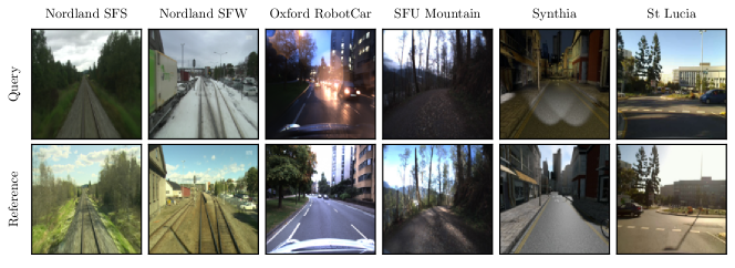
Figure 2: Sample images from the six VPR datasets employed in our research: These datasets encompass a diverse range of environments including urban locales undergoing seasonal transitions, varying illuminations from day to night, high-glare-induced illumination shifts, scenes with occlusions, railway lines, and forested areas.

We evaluate our work using several datasets that cover seasonal changes [50, 53], differences in the time of day [51, 52, 53], as well as rural [52, 50], suburban [54] and urban [51, 53] environments with additional challenges due to occlusions and glare [54]. We now briefly describe these datasets, and provide sample images in Figure 2.

The Nordland dataset [50]: captures a 728 km train path in Norway recorded in spring, summer, fall and winter. As commonly done in the literature [123, 124, 125], the data segments where the speed of the train is below 15km/h is removed using the provided GPS data. We subsampled places every 100 m approximately from the entire dataset obtaining 3300 places for each traverse. We trained our model on spring and fall traverses, and tested separately on summer and winter.

The Oxford RobotCar dataset [51]: has over 100 traverses captured in Oxford city and it is recorded at varying conditions including different time of the day, and different seasons. For each traverse, we subsampled places about every 10 m gaining 450 places. As done in prior works [126, 85], we selected sunny (2015-08-12-15-04-18) and rain (2015-10-29-12-18-17) traverses as the reference dataset and the dusk (2014-11-21-16-07-03) traverse as the query dataset.

The SFU-Mountain dataset [52]: has more than 8 hours of trail driving in Burnaby Mountain, British Columbia Canada, using the Clearpath Husky robot covering sunny, rainy and snowy conditions [52]. We used the dry traverse for reference and dusk traverse for query. We considered each image in the traverse as a different place, and used the author’s place sampling configurations [52], utilizing the entire dataset where each traverse contains 375 places.

The Synthia Night-to-Fall dataset [53]: was initially designed for semantic scene understanding in a city-like driving scenario, is a synthetic dataset. In our approach, following the methodology described in [127], we utilized the SEQS-04 foggy (reference) and nighttime (query) traverses. Segments in which the vehicle remained stationary were excluded, and we sampled approximately every 1 frame per second resulting in 275 places for each traverse.

The St Lucia dataset [54]: comprises several traverses along a route within the St Lucia suburb of Brisbane. For our experiments, we employed a traverse conducted during the early morning (reference; 190809-0845) and another in the late afternoon (query; 180809-1545). We omitted the segments in which the vehicle was at rest and sampled locations approximately every 20 meters, obtaining 350 places from the first half of the dataset.

IV-C Evaluation Metrics

We evaluate the performance of our method and baseline methods on all datasets using the recall at $N$ (R@$N$) evaluation metric, which considers a prediction as a correct match if at least one of the top $N$ predictions is within the ground truth tolerance [13, 127].

Let $P_{k}$ be the set of top $N$ predictions for the $k^{th}$ query and $G_{k}$ be the set of ground truth matches for the $k^{th}$ query within the specified tolerance. Let $\mathcal{Q}$ be the total number of queries. The recall at $N$ (R@$N$) can be defined as:

$$\text{R@}N=\frac{1}{Q}\sum_{k=1}^{Q}\mathds{1}\left(P_{k}\cap G_{k}\neq\emptyset\right),$$ (12)

where $\mathds{1}(\cdot)$ is the indicator function, which is $1$ if at least one of the top $N$ predictions for the $k^{th}$ query, $P_{k}$, is correctly matched to its ground truth $G_{k}$, and $0$ otherwise. We deem a query image as correctly paired only if it aligns exactly with the correct place.

IV-D Baseline Methods

We employ several conventional VPR approaches to evaluate the performance of our methods. These techniques encompass non-learned methods: Sum-of-Absolute-Differences (SAD) [39] and DenseVLAD [47], as well as deep learning-based methods: NetVLAD [46], AP-GeM [48], and Generalized Constrastive Loss (GCL) [49]. These approaches are detailed as follows:

Sum-of-Absolute-Differences (SAD) [39]: is a simple baseline technique which computes the pixel-wise difference between each query image and all reference images. While the sum-of-absolute differences method is simple, this method is not very robust to drastic varying conditions such as changes in lighting, viewpoint, and seasonal changes.

NetVLAD [46]: aggregates local image descriptors with learnable aggregation weights by employing the VLAD technique [97] to create a fixed-size global descriptor. We used the Pytorch NetVLAD implementation from [123], which has a VGG16 [128] backbone pretrained on ImageNet [129]. The NetVLAD layer, which is the pooling layer of the network, is trained on the Google Landmarks [130], Mapillary Street Level Sequences [131], and Pittsburgh [132] datasets separately. As NetVLAD is trained on urban environments, the model might not generalize well to completely different types of environments such as rural areas.

DenseVLAD [47]: utilizes densely sampled SIFT [133] image descriptors, and aggregates these features using VLAD [97]. We used the original MATLAB implementation of DenseVLAD. While DenseVLAD is very robust to high illumination, some limitations of DenseVLAD include lack of robustness to occlusions, very dark conditions with limited dynamic range, and rural areas with vegetation.

AP-GeM [48]: employs the Generalized-Mean pooling layer (GeM) [134] and uses a listwise loss formulation that directly optimizes for the Average Precision (AP) performance metric. We used the original Pytorch implementation of AP-GeM. This model uses a CNN-based backbone pretrained on ImageNet [129] to extract feature representations and aggregates it into a compact representation. We used three variations of AP-GeM; a ResNet50 backbone [135] trained on Landmarks-clean [136] dataset, a ResNet101 backbone [135] trained on Landmarks-clean [136] dataset, and a Res101 backbone [135] trained on Google-Landmarks Dataset [130]. Similar to NetVLAD, AP-GeM generalization is reliant on the type of environment used for training.

GCL [49]: is trained via a Generalized Contrastive Loss (GCL) using graded similarity labels for image pairs. We trained the last two layers of the network on the Mapillary Street-Level Sequences (MSLS) dataset [131] using a VGG16 backbone [128] pretrained on ImageNet [129] with GeM [134] as the pooling layer. We used the original Pytorch-based implementation of this model. GCL is currently a state-of-the-art VPR technique, robust to domain shift and fast to process.

IV-E Image Dimensions for Different Techniques

For GCL and NetVLAD, the images were resized to $640\times 480$ pixels, while for AP-GeM and DenseVLAD the native image resolutions were used (Nordland: $640\times 360$ pixels, Oxford RobotCar: $1280\times 960$ pixels, SFU-Mountain: $752\times 480$ pixels, Synthia Night To Fall: $300\times 200$ pixels, St Lucia: $640\times 480$ pixels). For SAD, the input images were patch-normalized and resized to $28\times 28$ pixels, matching the low-dimensional input image sizes that we used in our work.

IV-F Using Multiple Reference Traverses

For the Nordland and Oxford RobotCar datasets, we employed two reference traverses for training our SNN-based methods. For a fair comparison, we merged the VPR predictions from both traverses for these datasets by generating VPR predictions for the query based on each reference traverse to form one distance matrix per reference traverse. We then merged these distance matrices by selecting the minimum element-wise values.

V Results

TABLE I: R@1 performance comparisons of our Modular SNN and Ensembles of Modular SNNs to conventional VPR techniques with a sequence matcher at different sequence lengths (SL): SL1 (without a sequence matcher), SL2, SL4, and SL10. The best results are highlighted in bold, the second best results are underlined, and the third best results are italicized. The main key takeaways include: Our Ensemble of Modular SNNs 1) shows competitive performance, closely approaching that of leading VPR methods across various datasets, 2) obtains the highest R@1 improvement with a sequence matcher, compared to VPR techniques with similar-performing baselines except on Nordland, and 3) consistently outperforms the mean R@1 of its individual members across all datasets.

Datasets	Nordland (SFS)				Nordland (SFW)				Oxford RobotCar				SFU-Mountain				Synthia Night-To-Fall				St Lucia				Mean R@1
Method	SL1	SL2	SL4	SL10	SL1	SL2	SL4	SL10	SL1	SL2	SL4	SL10	SL1	SL2	SL4	SL10	SL1	SL2	SL4	SL10	SL1	SL2	SL4	SL10	SL1	SL2	SL4	SL10
NetVLAD (Landmarks)	0.79	0.92	0.97	1.00	0.22	0.35	0.52	0.77	0.43	0.54	0.68	0.89	0.43	0.52	0.69	0.95	0.72	0.78	0.85	0.86	0.41	0.57	0.75	0.94	0.50	0.61	0.74	0.90
NetVLAD (Mapillary)	0.71	0.87	0.96	1.00	0.17	0.28	0.46	0.71	0.45	0.59	0.75	0.93	0.36	0.48	0.58	0.85	0.64	0.71	0.83	0.86	0.46	0.65	0.82	1.00	0.47	0.60	0.73	0.89
NetVLAD (Pittsburgh)	0.62	0.82	0.95	0.99	0.14	0.22	0.36	0.59	0.52	0.67	0.83	0.97	0.45	0.61	0.80	0.97	0.69	0.78	0.83	0.86	0.37	0.57	0.76	0.98	0.47	0.61	0.76	0.89
AP-GeM (ResNet-50)	0.64	0.82	0.93	0.99	0.11	0.18	0.27	0.47	0.52	0.60	0.73	0.92	0.42	0.58	0.79	0.98	0.56	0.70	0.80	0.85	0.49	0.75	0.90	1.00	0.46	0.60	0.74	0.87
AP-GeM (ResNet-101)	0.67	0.84	0.94	0.99	0.08	0.11	0.15	0.27	0.54	0.64	0.79	0.95	0.44	0.59	0.77	0.98	0.57	0.67	0.79	0.84	0.48	0.65	0.87	1.00	0.46	0.58	0.72	0.84
AP-GeM (ResNet-101, LM18)	0.85	0.94	0.99	1.00	0.29	0.43	0.61	0.82	0.60	0.67	0.78	0.94	0.65	0.81	0.93	1.00	0.65	0.75	0.83	0.85	0.69	0.89	0.99	1.00	0.62	0.75	0.85	0.93
DenseVLAD	0.82	0.93	0.98	1.00	0.29	0.51	0.74	0.93	0.69	0.80	0.91	0.98	0.76	0.85	0.92	1.00	0.70	0.75	0.83	0.85	0.79	0.92	0.99	1.00	0.67	0.79	0.90	0.96
SAD	0.67	0.85	0.94	0.99	0.28	0.47	0.65	0.80	0.48	0.63	0.78	0.90	0.42	0.55	0.68	0.84	0.53	0.64	0.72	0.77	0.43	0.59	0.70	0.85	0.47	0.62	0.74	0.86
GCL	0.69	0.85	0.94	0.99	0.27	0.47	0.72	0.94	0.29	0.41	0.58	0.86	0.50	0.61	0.75	0.92	0.47	0.61	0.75	0.87	0.43	0.59	0.80	1.00	0.44	0.59	0.76	0.93
Modular SNN (Ours)	0.61	0.77	0.89	0.98	0.22	0.37	0.59	0.86	0.49	0.70	0.85	0.99	0.39	0.57	0.74	0.90	0.41	0.60	0.76	0.86	0.40	0.56	0.77	0.95	0.42	0.60	0.77	0.92
Ens of 3 AP-GeM	0.84	0.93	0.98	1.00	0.20	0.28	0.42	0.68	0.60	0.69	0.79	0.95	0.61	0.76	0.91	1.00	0.67	0.77	0.83	0.86	0.69	0.87	0.98	1.00	0.60	0.72	0.82	0.92
Ens of 3 GCL	0.69	0.85	0.94	0.99	0.29	0.51	0.76	0.96	0.28	0.41	0.57	0.81	0.50	0.62	0.77	0.92	0.51	0.59	0.76	0.86	0.41	0.60	0.82	1.00	0.45	0.60	0.77	0.92
Ens of 3 Modular SNNs (Ours)	0.70	0.84	0.93	0.99	0.31	0.46	0.67	0.91	0.59	0.80	0.95	1.00	0.47	0.69	0.85	0.97	0.47	0.63	0.77	0.86	0.45	0.67	0.87	0.99	0.50	0.68	0.84	0.95
Ens of 5 GCL	0.70	0.85	0.94	0.99	0.29	0.52	0.78	0.96	0.28	0.41	0.56	0.82	0.50	0.63	0.78	0.92	0.52	0.60	0.76	0.87	0.42	0.60	0.83	1.00	0.45	0.60	0.78	0.93
Ens of 5 Modular SNNs (Ours)	0.72	0.86	0.94	0.99	0.32	0.51	0.72	0.94	0.63	0.85	0.97	1.00	0.51	0.73	0.89	0.99	0.50	0.64	0.78	0.86	0.52	0.72	0.91	1.00	0.53	0.72	0.87	0.96

Section V-A analyzes how each component of our methodology affects the overall performance of the system. Subsequently, Section V-B compares the performance of our Ensemble of Modular SNNs without sequence matching against conventional VPR techniques. Section V-C extends this comparison to include sequence matching. Section V-D provides detailed analyses and introduces an indicator to assess the responsiveness of VPR techniques to sequence matching. We also provide an evaluation of the ensembling effect on our Modular SNN in Section V-E. This is followed by an ablation study on the effect of ensemble member randomization in our Ensemble of Modular SNNs in Section V-F. Finally, Section V-G concludes this section with an analysis of the computational efficiency and scalability aspects of our approach.

V-A Component-Wise Contributions to SNN Performance

This section overviews the performance contributions of each component of our approach, namely modularity (i.e. expert modules that learn small subsets of the reference dataset), ensembling (i.e. representing each place by multiple modules), and sequence matching (i.e. using multiple reference and query images for place matching). Figure 3 demonstrates that the performance of our Modular SNN is significantly increased when each of these techniques, ensembling (R@1 increase of 10.6%) and sequence matching (R@1 increase of 35.6% for a sequence length of four), is applied separately. Moreover, the combination of ensembling and sequence matching techniques further improves the R@1 of the Modular SNN (R@1 increase of 50.3%). As the ensembling and sequence matching techniques are commutative, the order of application of these two techniques produces identical outcomes. The Non-modular SNN by Hussaini et al. [85] performs poorly, even when ensembling and sequence matching are applied (R@1 is less than 0.2%).

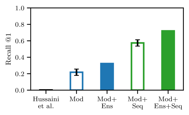
Figure 3: Component-wise ablation study: Introducing modularity (Mod) where multiple SNNs represent small subsets of the reference dataset enables large-scale place recognition, significantly outperforming the Non-modular baseline SNN by Hussaini et al. [85]. Both ensembling (five ensemble members; Mod+Ens) and sequence matching (sequence length four; Mod+Seq) individually enhance the R@1 of the Modular SNN, by 10.6% and 35.6% respectively. Their combined application further elevates the performance, surpassing the benefits of the individual techniques and resulting in a 50.3% R@1 improvement overall. Error bars indicate performance variations among the five ensemble members (standard deviation). The experiment was conducted on the Nordland dataset (Reference: Spring, Fall; query: Winter).

V-B Comparison of Ensemble of Modular SNNs without a Sequence Matcher to Conventional VPR Techniques

This section compares our Ensemble of Modular SNNs without a sequence matcher to the conventional VPR techniques outlined in Section IV-D on the datasets detailed in Section IV-B. As emphasized in [137], the efficacy of different visual place recognition methods fluctuates across different environments. The aim of our work is to demonstrate competitive but not necessarily state-of-the-art performance of our approach for visual place recognition.

Table I shows that our Ensemble of Modular SNNs consistently delivers competitive results, that are in close proximity to leading VPR methods across various datasets. This performance is noteworthy considering that AP-GeM (ResNet-101, LM18) and DenseVLAD are ranked as the top two VPR techniques on average over all datasets. It is worth noting that conventional VPR techniques have inherent advantages. They operate on much larger image dimensions as they falter with smaller image sizes which are used in our approach, and oftentimes benefit from extensive pretraining on large VPR datasets.

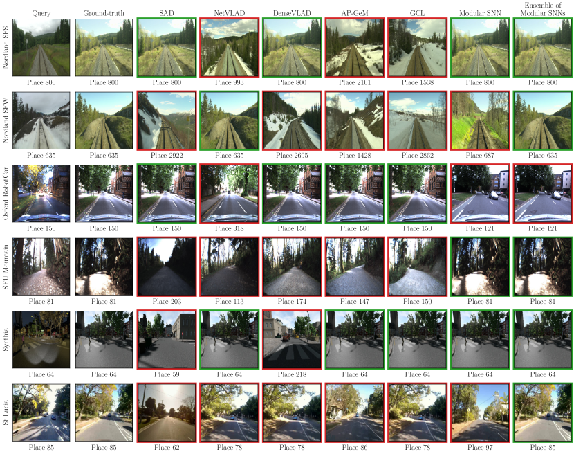
Figure 8: Qualitative results: The plot showcases the performance of our Standalone Modular SNN, Ensemble of Modular SNNs, and various VPR methods across diverse datasets. To enhance clarity, we have included just one of the three NetVLAD instances, specifically NetVLAD (Landmarks), and one of the three AP-GeM instances, namely AP-GeM (ResNet101, LM18). It details three instances of correct predictions by both Modular SNN and its Ensemble variant (in rows one, four, and five), two cases where the Ensemble yields correct matches despite the incorrect prediction of the Modular SNN as an ensemble member (in rows two and six), and a situation where both Modular and Ensemble of Modular SNNs fail to correctly match the query image to its corresponding reference image (in row three).

Figure 8 presents qualitative performance of our Modular SNN, Ensemble of Modular SNNs, and relevant VPR techniques used for comparison across all datasets, for both correct and incorrect prediction of query image instances.

(a)

(b)

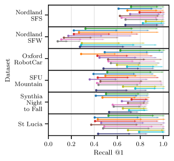
(c)

Figure 4: R@1 performance improvements with sequence matching: The plot shows the absolute R@1 performance improvement when employing sequence matchers using four (SL4) and ten (SL10) frames, compared to a single-frame approach (SL1). Dark to light shaded segments on the arrows reflect improvements with SL4 and SL10, respectively, with lengthier arrows signifying greater enhancements. We note that our proposed Ensemble of Modular SNNs (green) achieves the highest R@1 improvement with a sequence matcher compared to all other VPR techniques, with the exception of Nordland where GCL achieves slightly higher improvements.

V-C Comparison of Ensemble of Modular SNNs with a Sequence Matcher to Conventional VPR Techniques

This section extends the comparisons, this time incorporating a sequence matcher. Table I showcases the enhanced performance of our Ensemble of Modular SNNs as well as our standalone Modular SNN when integrated with a sequence matcher with a sequence length of two, four, and ten, separately, compared to conventional VPR techniques and/or their ensemble forms with a sequence matcher of same sequence lengths across all datasets.

Compared to VPR techniques with roughly similar baseline performance, our Ensemble of Modular SNNs obtains the highest improvement with a sequence matcher: the mean R@1 of our Ensemble of Modular SNNs with a sequence matcher across all datasets is among the top three models, despite the lower baseline performance without a sequence matcher. Specifically, Our Ensemble of Modular SNNs with a four-frame sequence matcher achieved a 37.2% R@1 performance gain on the SFU Mountain dataset with a baseline performance of 51.3%, surpassing the 25.7% increase of the comparable VPR technique, GCL, with a similar baseline performance of 49.6%. On the Oxford RobotCar dataset, before applying the sequence matcher, the R@1 of our model was 62.6%, comparable to the baseline performance of AP-GeM (ResNet101, LM18), which stood at 59.7%. Upon integrating the sequence matcher with four frames, the performance of our model surged to 96.5%, a significant increase that surpasses the post-sequence matching performance gains observed in AP-GeM (ResNet101, LM18), which reported an increase to 78.2%.

Figure 4 illustrates the R@1 of all techniques with a sequence matcher of sequence lengths four, and ten, via an arrow with different-colored shaded segments of dark, and light respectively. With the integration of a sequence matcher, our Ensemble of Modular SNNs achieves higher R@1 improvements over all other VPR methods, with the only exception being the Nordland dataset where GCL obtains marginally greater gains.

It is noteworthy that at longer sequence lengths, for example a sequence length of ten, the R@1 performance of all techniques converge towards perfect R@1 values, which makes it challenging to distinguish between the performances of these techniques with a sequence matcher. The variations in absolute performance gain of different techniques are more pronounced in shorter sequence lengths, offering clearer insights into the adaptability. Sequence matchers with shorter lengths are apt for indoor settings or high-speed contexts where successive visual scenes change swiftly, and reducing relocalization delays.

(a)

(b)

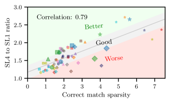
(c)

Figure 5: Indication of sequence matching responsiveness: The figure shows the correct match sparsity, defined as the standard deviation of the distances to the next correct match, against the R@1 performance ratio for sequence matcher lengths from four to one. A higher correct match sparsity indicates wider gaps between correct matches, suggesting that the method might be under performing or the dataset is challenging. The gray line represents the line of best fit, and a 20% error margin around this line is indicated with a gray shaded area. Data points in the green zone (above the diagonal) show greater responsiveness to sequence matching, while those in the red zone (below the diagonal) are less responsive. Both the proposed Standalone Modular SNN (larger blue points) and Ensemble of Modular SNNs (larger green points), primarily lie along or above the diagonal, showcasing their strong adaptability to sequence matching. Excluded from the analysis are outliers NetVLAD (Mapillary), NetVLAD (Pittsburgh), AP-GeM (ResNet-50), and AP-GeM (ResNet-101) on the Nordland winter query, with respective coordinates of (10.12, 2.63), (12.43, 2.69), (17.66, 2.43), and (23.41, 1.89) respectively, where all four outliers lie in the ‘Worse’ region.

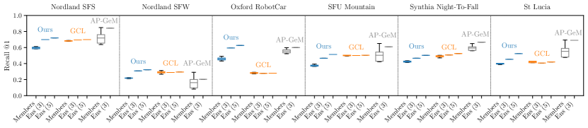
Figure 6: The effect of ensembling: The plot shows the R@1 performance of Ensembles of Modular SNNs (both with three, and five ensemble members; blue), GCL ensembles (both with three, and five ensemble members; orange), and an AP-GeM ensemble (with three ensemble members; gray) on all six evaluated datasets. Our Ensemble of Modular SNNs show superior R@1 performance over its individual members, while GCL ensembles exhibit minimal gains. The AP-GeM ensemble members have a varied R@1 performance spectrum, with the AP-GeM ensemble performance matching or falling short of its best-performing member across all datasets. For detailed metrics across all datasets, refer to Table I.

V-D An Indicator for Sequence Matching Responsiveness

This section examines whether the responsiveness of VPR techniques to sequence matching can be predicted, and offers insights that corroborate their respective behaviors. Specifically, we investigate how the sparsity of correct matches influences the R@1 performance when sequence matching is employed. Increased sparsity in correct matches denotes larger gaps between next correct matches due to limitations in the performance of a method or the intrinsic difficulty of the dataset.

To this end, Figure 5 presents the relationship between the standard deviation of the distance to the next correct match, which we define as the ‘Correct match sparsity’, and the R@1 performance ratio for a sequence matcher with a length of four against a sequence matcher with a length of one. The figure highlights three distinct regions differentiated by color: The plotted gray line signifies the line of best fit, and the gray area indicates a 20% margin around the line of best fit. The green region, situated above the diagonal, encapsulates techniques that exhibit a pronounced responsiveness to sequence matching on various datasets. Whereas, the red region, found below the diagonal, houses techniques that appear less influenced by sequence matching across various datasets.

Central to our discussion, the data points representing our Modular SNN, distinguished by their larger blue points, chiefly populate the vicinity of areas above the diagonal across all six datasets, emphasizing the robustness and adaptability of our Standalone Modular SNN to sequence matching. Similarly, our Ensemble of Modular SNNs, represented by their larger green points, has predominantly a high responsiveness to sequence matching, with most data points in the ‘Better’ region and close to it in the ‘Good’ region, suggesting robust performance, although a single point in the ‘Worse’ region indicates potential for improvement in specific scenarios. Compared to our Standalone Modular SNN, the higher baseline performance of our Ensemble of Modular SNNs exhibits less variability, hence, appears less responsive to sequence matching.

In general, techniques with higher performing baselines are less responsive to sequence matching. The VPR methods in this category include DenseVLAD, and AP-GeM (ResNet101, LM18) whose points mainly lie in the ‘Good’ region, with a few cases in the ‘Worse’ region. The conventional VPR technique GCL, which generally displays high responsiveness to sequence matching with its data points concentrated in the ‘Better’ and ‘Good’ regions, is on par with our Ensemble of Modular SNNs in performance, except on Oxford RobotCar and SFU Mountain datasets in which our method is more responsive, and on St Lucia dataset where GCL is more responsive due to the higher baseline performance of our method. Our Ensemble of Modular SNNs, despite its overall higher baseline performance compared to GCL, achieves greater sequence matching responsiveness than GCL, which is a significant accomplishment as increased responsiveness is challenging to attain with an already high-performing baseline. We note that we excluded 4 outlier points to better observe the general trends in the data and understand overall performance characteristics; these are detailed in the Figure 5 caption.

V-E Ensembling: How Much Does It Help?

This section evaluates the effect of ensembling on our Modular SNN, and provides comparisons to GCL and AP-GeM ensembles. The ensemble members in the case of our Modular SNN are homogeneous as they share the same network architecture and training data; their differences lie in the random initialization values of weights and the random sequence of input images, as elaborated in Section III-D. The GCL ensembles are also homogeneous with consistent network architecture and training datasets and only differing in random initialization of weights and order of input images. The AP-GeM ensembles are heterogeneous, showing diverse Convolutional Neural Network (CNN) backbone and/or training datasets. The three architectures are a ResNet50 and a ResNet101, both trained on the Landmarks-clean dataset, and a Res101 trained on the Google-Landmarks Dataset, as described in Section IV-D.

Figure 6 presents the R@1 performance improvement of our Ensemble of Modular SNNs (both with three, and five ensemble members), ensemble of GCL (both with three, and five ensemble members), and an ensemble of AP-GeM models (with three ensemble members) relative to the mean R@1 of their respective ensemble members across all datasets. Individual Modular SNNs perform relatively consistent with little variation in R@1 performance. The Ensemble of Modular SNNs (both with three, and five ensemble members) consistently outperforms the average R@1 of its individual members. Across all datasets, the ensembles with three members achieve an average R@1 of 49.8%, compared to their individual members’ mean R@1 of 41.4%. Similarly, ensembles with five members reach an average R@1 of 53.5%, exceeding their members’ mean R@1 of 41.1%.

While the homogeneous GCL ensemble members achieve consistent R@1 performance, which is similar to the consistency in performance of our Modular SNN ensemble members, the GCL ensemble (both with three, and five ensemble members) shows little to no improvement in R@1 over its individual member average (R@1 improvements of less than 2%) in both three and five ensemble member instances.

The ensemble members of the heterogeneous AP-GeM models exhibit a wide range of R@1 performance. The ensemble performance is equal to and/or inferior to the R@1 of the best-performing ensemble member across all six datasets (see Table I). Across all datasets, the mean R@1 for the ensemble is 60.1%, falling below the 62.1% R@1 of the top-performing member, AP-GeM (ResNet-101, LM18), even though the average R@1 of the ensemble members is 51.4%. Consequently, applying the ensembling technique to these AP-GeM models diminishes the performance of the best-performing member.

V-F Ablation Study on Member Randomization in Ensemble of Modular SNNs

This section provides an ablation study on the R@1 performance of our Ensemble of Modular SNNs with and without input image order shuffling, and with and without different random weight initialization that is applied to the ensemble members. In our previous conference paper [55], we provided consecutive input images of a traverse to the modules for training. We initialized the weights of all modules using the same random values. Here, to increase the diversity among the ensemble members, we instead shuffled the reference images of each traverse for the training process, and then fed these shuffled images to the modules (Figure 1). Moreover, we initialized the weights of each member, Modular SNN, using different random values, while within each member, using the same set of random values for all modules.

TABLE II: Ablation study on Ensemble of three Modular SNNs with and without randomization of initial weights, and shuffled order of images on the Nordland (Reference: Spring, Fall; query: Summer) dataset. Best configuration is in bold.

Randomized Weights	Shuffled Order	R@1
$\times$	$\times$	0.54
$\checkmark$	$\times$	0.66
$\times$	$\checkmark$	0.69
$\checkmark$	$\checkmark$	0.70

Table II presents the R@1 performance of these four ensemble variants on the Nordland dataset (Reference: Spring, Fall; query: Summer), where each ensemble contains three ensemble members. The first variant is an ensemble model where no randomization is not applied, resulting in identical ensemble members and thus mirroring the performance of a single member, which is 53.7%. The ensemble members in the second variant differ only in their initial random weights, resulting in a R@1 of 65.6%, with the mean R@1 performance of ensemble members being 55.3%. The third variant varies the ensemble members with only in the shuffled order of images, yielding in a R@1 performance of 68.9%, with a mean ensemble member R@1 performance of 58.7%. Lastly, the fourth variant combines both randomization of weights and shuffled order of images, producing the highest R@1 performance of 69.8%, with the mean R@1 performance of ensemble members being 59.6%.

Excluding the first variant, which negates the ensembling effect, the remaining three variants show similar R@1 performance improvements over their mean R@1 member performances. Randomizing the shuffled order of images significantly enhances ensemble performance compared to just randomizing the weights. The combination of both strategies obtains the highest R@1, albeit with a marginal improvement over the third variant, where only shuffled order of images are randomized.

V-G Compute and Scalability

Figure 7 provides insights into the scalability and computational efficiency of our Modular and Ensemble of Modular SNNs with two ensemble members, against the Non-modular SNN from [85]. The plot shows that the query times of our Modular SNN and Ensemble of Modular SNNs scale linearly as the number of learned places increases. Meanwhile, the Non-modular SNN faces scalability issues beyond 400 places. We anticipate that implementing our Modular and Ensemble of Modular SNNs on neuromorphic hardware could substantially enhance processing speed through hardware parallelism. This is one of our future research directions, as described in more detail in Section VI.

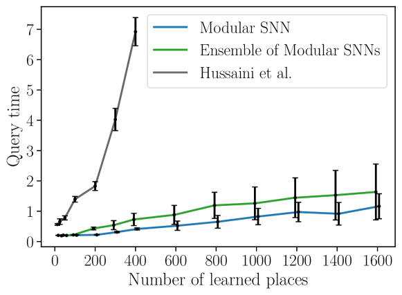
Figure 7: Performance scalability comparison: We show the average query processing time for a single query image as the number of places (and thus overall network size) increases. We contrast our Modular and Ensemble of Modular SNNs with two ensemble members, with the approach from [85]. Both the Modular SNN and Ensemble of Modular SNNs demonstrate to scale linearly with the number of reference places. In contrast, the Non-modular SNN did not scale well, and we were only able to test up to 6400 output neurons (400 places). We expect both our Ensemble and non-Ensemble variants to scale even better and yield even lower inference times on neuromorphic hardware due to their massive parallel processing capabilities.

VI Discussions and Conclusions

This paper has shed light on the capabilities of spiking neural networks (SNNs) in the realm of visual place recognition. Through a series of enhancements, we have showcased their utility and promise in this field.

Firstly, we introduced scalable SNNs that we dubbed Modular SNNs which represent a small region of the environment and have enhanced adaptability and efficiency in expansive environments. This innovation significantly broadens the applicability of SNNs for place recognition tasks.

Building on the foundation of Modular SNNs, we further enhanced our approach by introducing the Ensemble of Modular SNNs in our second contribution. In this case, multiple SNNs are employed to represent a single place, which demonstrated a substantial improvement in place recognition robustness and generalization ability. We have shown that the responsiveness of SNNs to ensembling is higher compared to conventional techniques that employed homogeneous and heterogeneous ensembles. This is evident as the average R@1 of our Ensemble of Modular SNNs across all datasets is consistently higher than the average R@1 of its ensemble members, highlighting that the ensembling technique significantly amplifies the capabilities of our Modular SNN approach. Moreover, our Ensemble of Modular SNNs has demonstrated competitive performance, in close proximity with the leading VPR methods, across various datasets.

Lastly, in addition to ensembling, we also explored the impact of sequence matching, a technique that further augments our system’s performance by utilizing multiple consecutive images for place matching. Pairing our Ensemble of Modular SNNs with sequence matching exhibited a higher R@1 performance improvement compared to VPR techniques with similar baselines, except in the case of the Nordland dataset. This reinforces the transformative role of sequence matching on enhancing SNN capabilities for visual place recognition. We also provided an indicator for sequence matching responsiveness, applicable to general VPR techniques, which demonstrated the competitive adaptability of our SNN-based solutions to sequence matching compared to that of VPR techniques.

Our work follows the similar trend seen in the recent state-of-the-art conventional VPR techniques such as [99] that frame the visual place recognition problem as a classification task, enabling large-scale recognition capability by bypassing the computationally heavy process of computing the pairwise distance matrix for all query and reference feature representations. Another benefit of approaching the VPR problem as a classification task is that it eliminates the need to divide the reference and query datasets into separate training and testing partitions, effectively circumventing the potential complication of overlapping data in the training and testing subsets [99]. Furthermore, we demonstrate the performance of our SNN approach using low resolution image sizes, which scales well with increasing number of places in terms of storage complexity. In comparison, conventional VPR techniques typically need to store reference image feature descriptors, posing challenges for scaling to large datasets due to associated increase in storage requirements.

Looking ahead, our future work aims to leverage these findings and explore new frontiers in neuromorphic computing. We plan to implement our approach on specialized neuromorphic hardware platforms, particularly Intel’s Loihi 2, to harness its inherent advantages in obtaining high energy efficiency and reduced latency. Although ensemble methods often face scalability issues, we see potential in neuromorphic computing, known for its exceptional parallel processing capabilities, to address these concerns. A limitation of our work is the minimal robustness to viewpoint shift, an aspect that most VPR techniques address effectively. Enhancing the resilience of our system to viewpoint change remains a priority for us, as it is crucial for reliable place recognition in more challenging situations. However, the necessity for robustness against significant viewpoint shifts may vary depending on the specific downstream application of our visual place recognition system. For instance, in scenarios where the VPR system acts as a loop closure component of a Simultaneous Localization and Mapping (SLAM) process, the limitations of SLAM system in loop closure might render extreme viewpoint robustness less critical [16]. We are also exploring the possibility of using event cameras to directly input event data to further enhance energy efficiency and reduce latency, moving away from our current strategy of converting traditional image data to rate-coded event streams.

Our research illuminates the significant potential of SNNs for robotic navigation, presenting a solution that is scalable, responsive, and robust for place recognition tasks. These advancements in SNN technology not only enhance the efficiency of robotic navigation systems but also have vast applicability across various real-world robotics applications. Our findings are particularly promising for resource-constrained robots, such as those deployed in challenging environments like space and underwater, where the focus on edge computing and considerations for SWaP (Size, Weight, and Power) underscore its suitability for these rigorous settings.

References

- [1] S. Ghosh-Dastidar and H. Adeli, “Spiking neural networks,” Int. J. Neural Syst., vol. 19, no. 04, pp. 295–308, 2009.
- [2] Y. Sandamirskaya, M. Kaboli, J. Conradt, and T. Celikel, “Neuromorphic computing hardware and neural architectures for robotics,” Sci. Robot., vol. 7, no. 67, p. eabl8419, 2022.
- [3] C. D. Schuman et al., “Opportunities for neuromorphic computing algorithms and applications,” Nat. Comput. Sci., vol. 2, no. 1, pp. 10–19, 2022.
- [4] K. Yamazaki, V.-K. Vo-Ho, D. Bulsara, and N. Le, “Spiking neural networks and their applications: A review,” Brain Sci., vol. 12, no. 7, p. 863, 2022.
- [5] W. Gerstner, W. M. Kistler, R. Naud, and L. Paninski, Neuronal dynamics: From single neurons to networks and models of cognition. Cambridge University Press, 2014.
- [6] J. D. Nunes, M. Carvalho, D. Carneiro, and J. S. Cardoso, “Spiking neural networks: A survey,” IEEE Access, vol. 10, pp. 60 738–60 764, 2022.
- [7] E. P. Frady et al., “Neuromorphic nearest neighbor search using Intel’s Pohoiki Springs,” in Proc. Neuro-inspired Comput. Elements Worksh., 2020.
- [8] M. Davies et al., “Advancing neuromorphic computing with Loihi: A survey of results and outlook,” Proc. IEEE, vol. 109, no. 5, pp. 911–934, 2021.
- [9] J. Pei, , et al., “Towards artificial general intelligence with hybrid Tianjic chip architecture,” Nature, vol. 572, no. 7767, pp. 106–111, 2019.
- [10] S. B. Furber, F. Galluppi, S. Temple, and L. A. Plana, “The SpiNNaker project,” Proc. IEEE, vol. 102, no. 5, pp. 652–665, 2014.
- [11] J. Yik, S. H. Ahmed, et al., “NeuroBench: Advancing neuromorphic computing through collaborative, fair and representative benchmarking,” arXiv preprint arXiv:2304.04640, 2023.
- [12] J. K. Eshraghian et al., “Training spiking neural networks using lessons from deep learning,” Proc. IEEE, 2023.
- [13] S. Schubert, P. Neubert, S. Garg, M. Milford, and T. Fischer, “Visual place recognition: A tutorial,” IEEE Robotics & Automation Magazine, 2023.
- [14] S. Garg, T. Fischer, and M. Milford, “Where is your place, visual place recognition?” in Int. Jt. Conf. Artif. Intell., 2021, pp. 4416–4425.
- [15] S. Lowry, N. Sünderhauf, P. Newman, J. J. Leonard, D. Cox, P. Corke, and M. J. Milford, “Visual place recognition: A survey,” IEEE Trans. Robot., vol. 32, no. 1, pp. 1–19, 2015.
- [16] K. A. Tsintotas, L. Bampis, and A. Gasteratos, “Visual place recognition for simultaneous localization and mapping,” Autonomous Vehicles Volume 2: Smart Vehicles, pp. 47–79, 2022.
- [17] C. Masone and B. Caputo, “A survey on deep visual place recognition,” IEEE Access, vol. 9, pp. 19 516–19 547, 2021.
- [18] X. Zhang, L. Wang, and Y. Su, “Visual place recognition: A survey from deep learning perspective,” Pattern Recognit., vol. 113, p. 107760, 2021.
- [19] C. Cadena et al., “Past, present, and future of simultaneous localization and mapping: Toward the robust-perception age,” IEEE Trans. Robot., vol. 32, no. 6, pp. 1309–1332, 2016.
- [20] G. Auda and M. Kamel, “Modular neural networks: a survey,” Int. J. Neural Syst., vol. 9, no. 02, pp. 129–151, 1999.
- [21] T. Räuker, A. Ho, S. Casper, and D. Hadfield-Menell, “Toward transparent AI: A survey on interpreting the inner structures of deep neural networks,” in IEEE Conf. Secure Trustworthy Mach. Learn., 2023, pp. 464–483.
- [22] M. Amer and T. Maul, “A review of modularization techniques in artificial neural networks,” Artif. Intell. Rev., vol. 52, pp. 527–561, 2019.
- [23] M. Colosi et al., “Plug-and-play SLAM: A unified SLAM architecture for modularity and ease of use,” in IEEE/RSJ Int. Conf. Intell. Robot. Syst., 2020, pp. 5051–5057.
- [24] R. Dubé et al., “Segmatch: Segment based place recognition in 3D point clouds,” in IEEE Int. Conf. Robot. Autom., 2017, pp. 5266–5272.
- [25] S. Garg, A. Jacobson, S. Kumar, and M. Milford, “Improving condition-and environment-invariant place recognition with semantic place categorization,” in IEEE/RSJ Int. Conf. Intell. Robot. Syst., 2017, pp. 6863–6870.
- [26] J.-L. Blanco-Claraco, “A modular optimization framework for localization and mapping.” in Robot. Sci. Syst., 2019.
- [27] M. A. Ganaie, M. Hu, A. Malik, M. Tanveer, and P. Suganthan, “Ensemble deep learning: A review,” Eng. Appl. Artif. Intell., vol. 115, p. 105151, 2022.
- [28] W. Li, Y. Peng, M. Zhang, L. Ding, H. Hu, and L. Shen, “Deep model fusion: A survey,” arXiv preprint arXiv:2309.15698, 2023.
- [29] Y. Yang, H. Lv, and N. Chen, “A survey on ensemble learning under the era of deep learning,” Artif. Intell. Rev., vol. 56, no. 6, pp. 5545–5589, 2023.
- [30] T. G. Dietterich, “Ensemble methods in machine learning,” in Int. Worksh. Multiple Classifier Syst., 2000, pp. 1–15.
- [31] Z.-H. Zhou, Ensemble methods: foundations and algorithms. CRC press, 2012.
- [32] O. Sagi and L. Rokach, “Ensemble learning: A survey,” Wiley Interdiscip. Rev. Data Min. Knowl. Discov., vol. 8, no. 4, p. e1249, 2018.
- [33] Y. Wu, Y. Zhang, D. Zhu, Y. Feng, S. Coleman, and D. Kerr, “EAO-SLAM: Monocular semi-dense object SLAM based on ensemble data association,” in IEEE/RSJ Int. Conf. Intell. Robot. Syst., 2020, pp. 4966–4973.
- [34] M. J. Procopio, J. Mulligan, and G. Grudic, “Learning terrain segmentation with classifier ensembles for autonomous robot navigation in unstructured environments,” J. Field Robot., vol. 26, no. 2, pp. 145–175, 2009.
- [35] B. Arcanjo et al., “A-music: An adaptive ensemble system for visual place recognition in changing environments,” arXiv preprint arXiv:2303.14247, 2023.
- [36] C. Malone, S. Hausler, T. Fischer, and M. Milford, “Boosting performance of a baseline visual place recognition technique by predicting the maximally complementary technique,” in IEEE Int. Conf. Robot. Autom., 2023, pp. 1919–1925.
- [37] T. Fischer and M. Milford, “Event-based visual place recognition with ensembles of temporal windows,” IEEE Robot. Autom. Lett., vol. 5, no. 4, pp. 6924–6931, 2020.
- [38] B. Lakshminarayanan, A. Pritzel, and C. Blundell, “Simple and scalable predictive uncertainty estimation using deep ensembles,” Adv. Neural Inform. Process. Syst., vol. 30, 2017.
- [39] M. J. Milford and G. F. Wyeth, “SeqSLAM: Visual route-based navigation for sunny summer days and stormy winter nights,” in IEEE Int. Conf. Robot. Autom., 2012, pp. 1643–1649.
- [40] S. Garg and M. Milford, “SeqNet: Learning descriptors for sequence-based hierarchical place recognition,” IEEE Robot. Autom. Lett., vol. 6, no. 3, pp. 4305–4312, 2021.
- [41] S. Garg, M. Vankadari, and M. Milford, “SeqMatchNet: Contrastive learning with sequence matching for place recognition & relocalization,” in Conference on Robot Learning, 2022, pp. 429–443.
- [42] S. Schubert, P. Neubert, and P. Protzel, “Fast and memory efficient graph optimization via icm for visual place recognition.” in Robot. Sci. Syst., vol. 73, 2021.
- [43] R. Mereu, G. Trivigno, G. Berton, C. Masone, and B. Caputo, “Learning sequential descriptors for sequence-based visual place recognition,” IEEE Robot. Autom. Lett., vol. 7, no. 4, pp. 10 383–10 390, 2022.
- [44] J. M. Facil, D. Olid, L. Montesano, and J. Civera, “Condition-invariant multi-view place recognition,” arXiv preprint arXiv:1902.09516, 2019.
- [45] T. Naseer, M. Ruhnke, C. Stachniss, L. Spinello, and W. Burgard, “Robust visual SLAM across seasons,” in IEEE/RSJ Int. Conf. Intell. Robot. Syst., 2015, pp. 2529–2535.
- [46] R. Arandjelovic, P. Gronat, A. Torii, T. Pajdla, and J. Sivic, “NetVLAD: CNN architecture for weakly supervised place recognition,” IEEE Trans. Pattern Anal. Mach. Intell., vol. 40, no. 6, pp. 1437–1451, 2018.
- [47] A. Torii, R. Arandjelovic, J. Sivic, M. Okutomi, and T. Pajdla, “24/7 place recognition by view synthesis,” in IEEE Conf. Comput. Vis. Pattern Recog., 2015, pp. 1808–1817.
- [48] J. Revaud, J. Almazán, R. S. Rezende, and C. R. d. Souza, “Learning with average precision: Training image retrieval with a listwise loss,” in Int. Conf. Comput. Vis., 2019, pp. 5107–5116.
- [49] M. Leyva-Vallina, N. Strisciuglio, and N. Petkov, “Data-efficient large scale place recognition with graded similarity supervision,” in IEEE Conf. Comput. Vis. Pattern Recog., 2023, pp. 23 487–23 496.
- [50] N. Sünderhauf, P. Neubert, and P. Protzel, “Are we there yet? Challenging SeqSLAM on a 3000 km journey across all four seasons,” in IEEE Int. Conf. Robot. Autom. Worksh., 2013.
- [51] W. Maddern, G. Pascoe, C. Linegar, and P. Newman, “1 year, 1000 km: The Oxford RobotCar dataset,” Int. J. Robot. Res., vol. 36, no. 1, pp. 3–15, 2017.
- [52] J. Bruce, J. Wawerla, and R. Vaughan, “The SFU mountain dataset: Semi-structured woodland trails under changing environmental conditions,” in IEEE Int. Conf. Robot. Autom., 2015.
- [53] G. Ros, L. Sellart, J. Materzynska, D. Vazquez, and A. M. Lopez, “The synthia dataset: A large collection of synthetic images for semantic segmentation of urban scenes,” in IEEE Conf. Comput. Vis. Pattern Recog., 2016, pp. 3234–3243.
- [54] M. J. Milford and G. F. Wyeth, “Mapping a suburb with a single camera using a biologically inspired SLAM system,” IEEE Trans. Robot., vol. 24, no. 5, pp. 1038–1053, 2008.
- [55] S. Hussaini, M. Milford, and T. Fischer, “Ensembles of compact, region-specific & regularized spiking neural networks for scalable place recognition,” in IEEE Int. Conf. Robot. Autom., 2023, pp. 4200–4207.
- [56] B. Rueckauer, I.-A. Lungu, Y. Hu, M. Pfeiffer, and S.-C. Liu, “Conversion of continuous-valued deep networks to efficient event-driven networks for image classification,” Front. Neurosci., vol. 11, p. 682, 2017.
- [57] T. Bu, W. Fang, J. Ding, P. DAI, Z. Yu, and T. Huang, “Optimal ANN-SNN conversion for high-accuracy and ultra-low-latency spiking neural networks,” in Int. Conf. Learn. Represent., 2021.
- [58] J. Ding, Z. Yu, Y. Tian, and T. Huang, “Optimal ANN-SNN conversion for fast and accurate inference in deep spiking neural networks,” in Int. Jt. Conf. Artif. Intell., 2021.
- [59] E. Hunsberger and C. Eliasmith, “Training spiking deep networks for neuromorphic hardware,” arXiv preprint arXiv:1611.05141, 2016.
- [60] W. Severa, C. M. Vineyard, R. Dellana, S. J. Verzi, and J. B. Aimone, “Training deep neural networks for binary communication with the whetstone method,” Nat. Mach. Intell., vol. 1, no. 2, pp. 86–94, 2019.
- [61] C. Stöckl and W. Maass, “Optimized spiking neurons can classify images with high accuracy through temporal coding with two spikes,” Nat. Mach. Intell., vol. 3, no. 3, pp. 230–238, 2021.
- [62] C. Lee, S. S. Sarwar, P. Panda, G. Srinivasan, and K. Roy, “Enabling spike-based backpropagation for training deep neural network architectures,” Front. Neurosci., p. 119, 2020.
- [63] A. Renner, F. Sheldon, A. Zlotnik, L. Tao, and A. Sornborger, “The backpropagation algorithm implemented on spiking neuromorphic hardware,” arXiv preprint arXiv:2106.07030, 2021.
- [64] G. Shen, D. Zhao, and Y. Zeng, “Backpropagation with biologically plausible spatiotemporal adjustment for training deep spiking neural networks,” Patterns, vol. 3, no. 6, 2022.
- [65] G.-q. Bi and M.-m. Poo, “Synaptic modifications in cultured hippocampal neurons: dependence on spike timing, synaptic strength, and postsynaptic cell type,” J. Neurosci., vol. 18, no. 24, pp. 10 464–10 472, 1998.
- [66] P. U. Diehl and M. Cook, “Unsupervised learning of digit recognition using spike-timing-dependent plasticity,” Front. Comput. Neurosci., vol. 9, no. 99, pp. 1–9, 2015.
- [67] I. Abadía, F. Naveros, E. Ros, R. R. Carrillo, and N. R. Luque, “A cerebellar-based solution to the nondeterministic time delay problem in robotic control,” Sci. Robot., vol. 6, no. 58, p. eabf2756, 2021.
- [68] A. Vitale, A. Renner, C. Nauer, D. Scaramuzza, and Y. Sandamirskaya, “Event-driven vision and control for UAVs on a neuromorphic chip,” in IEEE Int. Conf. Robot. Autom., 2021, pp. 103–109.
- [69] J. Dupeyroux, J. J. Hagenaars, F. Paredes-Vallés, and G. C. de Croon, “Neuromorphic control for optic-flow-based landing of mavs using the loihi processor,” in IEEE Int. Conf. Robot. Autom., 2021, pp. 96–102.
- [70] R. K. Stagsted et al., “Event-based PID controller fully realized in neuromorphic hardware: A one DoF study,” in IEEE/RSJ Int. Conf. Intell. Robot. Syst., 2020, pp. 10 939–10 944.
- [71] J. Ding et al., “Biologically inspired dynamic thresholds for spiking neural networks,” Adv. Neural Inform. Process. Syst., vol. 35, pp. 6090–6103, 2022.
- [72] J. C. V. Tieck et al., “Towards grasping with spiking neural networks for anthropomorphic robot hands,” in IEEE Int. Conf. Artif. Neural Netw., 2017, pp. 43–51.
- [73] J. C. V. Tieck, L. Steffen, J. Kaiser, A. Roennau, and R. Dillmann, “Controlling a robot arm for target reaching without planning using spiking neurons,” in Int. Conf. Cogn. Inform. Cogn. Comput., 2018, pp. 111–116.
- [74] K. M. Oikonomou, I. Kansizoglou, and A. Gasteratos, “A hybrid spiking neural network reinforcement learning agent for energy-efficient object manipulation,” Machines, vol. 11, no. 2, p. 162, 2023.
- [75] A. Lele, Y. Fang, J. Ting, and A. Raychowdhury, “An end-to-end spiking neural network platform for edge robotics: From event-cameras to central pattern generation,” IEEE Trans. Cogn. Develop. Syst., vol. 14, no. 3, pp. 1092–1103, 2021.
- [76] Y. Luo, H. Shen, X. Cao, T. Wang, Q. Feng, and Z. Tan, “Conversion of siamese networks to spiking neural networks for energy-efficient object tracking,” Neural. Comput. Appl., vol. 34, no. 12, pp. 9967–9982, 2022.
- [77] R. Kreiser, A. Renner, V. R. Leite, B. Serhan, C. Bartolozzi, A. Glover, and Y. Sandamirskaya, “An on-chip spiking neural network for estimation of the head pose of the iCub robot,” Front. Neurosci., vol. 14, p. 551, 2020.
- [78] A. Renner et al., “Neuromorphic visual scene understanding with resonator networks,” arXiv preprint arXiv:2208.12880, 2022.
- [79] M. J. Milford, G. F. Wyeth, and D. Prasser, “RatSLAM: a hippocampal model for simultaneous localization and mapping,” in IEEE Int. Conf. Robot. Autom., 2004, pp. 403–408.
- [80] F. Galluppi et al., “Live demo: Spiking RatSLAM: Rat hippocampus cells in spiking neural hardware,” in IEEE Biomed. Circuits Syst. Conf., 2012, pp. 91–91.
- [81] G. Tang and K. P. Michmizos, “Gridbot: An autonomous robot controlled by a spiking neural network mimicking the brain’s navigational system,” in Int. Conf. Neuromorphic Syst., 2018, pp. 1–8.
- [82] R. Kreiser, A. Renner, Y. Sandamirskaya, and P. Pienroj, “Pose estimation and map formation with spiking neural networks: towards neuromorphic SLAM,” in IEEE/RSJ Int. Conf. Intell. Robot. Syst., 2018, pp. 2159–2166.
- [83] G. Tang, A. Shah, and K. P. Michmizos, “Spiking neural network on neuromorphic hardware for energy-efficient unidimensional SLAM,” in IEEE/RSJ Int. Conf. Intell. Robot. Syst., 2019, pp. 4176–4181.
- [84] N. S.-Y. Dumont, P. M. Furlong, J. Orchard, and C. Eliasmith, “Exploiting semantic information in a spiking neural SLAM system,” Front. Neurosci., vol. 17, 2023.
- [85] S. Hussaini, M. Milford, and T. Fischer, “Spiking neural networks for visual place recognition via weighted neuronal assignments,” IEEE Robot. Autom. Lett., vol. 7, no. 2, pp. 4094–4101, 2022.
- [86] R. Kreiser, M. Cartiglia, J. N. Martel, J. Conradt, and Y. Sandamirskaya, “A neuromorphic approach to path integration: a head-direction spiking neural network with vision-driven reset,” in IEEE Int. Symp. Circuits Syst., 2018, pp. 1–5.
- [87] R. Kreiser, G. Waibel, N. Armengol, A. Renner, and Y. Sandamirskaya, “Error estimation and correction in a spiking neural network for map formation in neuromorphic hardware,” in IEEE Int. Conf. Robot. Autom., 2020, pp. 6134–6140.
- [88] A. Safa, T. Verbelen, I. Ocket, A. Bourdoux, H. Sahli, F. Catthoor, and G. Gielen, “Fusing event-based camera and radar for SLAM using spiking neural networks with continual STDP learning,” in IEEE Int. Conf. Robot. Autom., 2023, pp. 2782–2788.
- [89] M. Milford, H. Kim, M. Mangan, S. Leutenegger, T. Stone, B. Webb, and A. Davison, “Place recognition with event-based cameras and a neural implementation of SeqSLAM,” arXiv preprint arXiv:1505.04548, 2015.
- [90] D. Weikersdorfer, R. Hoffmann, and J. Conradt, “Simultaneous localization and mapping for event-based vision systems,” in Int. Conf. Comput. Vis. Syst., 2013, pp. 133–142.
- [91] A. R. Vidal, H. Rebecq, T. Horstschaefer, and D. Scaramuzza, “Ultimate SLAM? Combining events, images, and imu for robust visual SLAM in HDR and high-speed scenarios,” IEEE Robot. Autom. Lett., vol. 3, no. 2, pp. 994–1001, 2018.
- [92] T. Fischer and M. Milford, “How many events do you need? Event-based visual place recognition using sparse but varying pixels,” IEEE Robot. Autom. Lett., vol. 7, no. 4, pp. 12 275–12 282, 2022.
- [93] G. Gallego et al., “Event-based vision: A survey,” IEEE Trans. Pattern Anal. Mach. Intell., vol. 44, no. 1, pp. 154–180, 2020.
- [94] M. Xu, N. Snderhauf, and M. Milford, “Probabilistic visual place recognition for hierarchical localization,” IEEE Robot. Autom. Lett., vol. 6, no. 2, pp. 311–318, 2020.
- [95] M. Cummins and P. Newman, “Fab-map: Probabilistic localization and mapping in the space of appearance,” Int. J. Robot. Res., vol. 27, no. 6, pp. 647–665, 2008.
- [96] A.-D. Doan, Y. Latif, T.-J. Chin, Y. Liu, T.-T. Do, and I. Reid, “Scalable place recognition under appearance change for autonomous driving,” in Int. Conf. Comput. Vis., 2019, pp. 9319–9328.
- [97] H. Jégou, M. Douze, C. Schmid, and P. Pérez, “Aggregating local descriptors into a compact image representation,” in IEEE Conf. Comput. Vis. Pattern Recog., 2010, pp. 3304–3311.
- [98] G. Trivigno, G. Berton, J. Aragon, B. Caputo, and C. Masone, “Divide&classify: Fine-grained classification for city-wide visual geo-localization,” in Int. Conf. Comput. Vis., 2023, pp. 11 142–11 152.
- [99] G. Berton, C. Masone, and B. Caputo, “Rethinking visual geo-localization for large-scale applications,” in IEEE Conf. Comput. Vis. Pattern Recog., 2022, pp. 4878–4888.
- [100] P.-E. Sarlin, C. Cadena, R. Siegwart, and M. Dymczyk, “From coarse to fine: Robust hierarchical localization at large scale,” in IEEE Conf. Comput. Vis. Pattern Recog., 2019, pp. 12 716–12 725.
- [101] C. Fan, Z. Chen, A. Jacobson, X. Hu, and M. Milford, “Biologically-inspired visual place recognition with adaptive multiple scales,” Robo. and Auton. sys., vol. 96, pp. 224–237, 2017.
- [102] S. Hausler and M. Milford, “Hierarchical multi-process fusion for visual place recognition,” in IEEE Int. Conf. Robot. Autom., 2020, pp. 3327–3333.
- [103] N. V. Keetha, M. Milford, and S. Garg, “A hierarchical dual model of environment-and place-specific utility for visual place recognition,” IEEE Robot. Autom. Lett., vol. 6, no. 4, pp. 6969–6976, 2021.
- [104] E. Garcia-Fidalgo and A. Ortiz, “Hierarchical place recognition for topological mapping,” IEEE Trans. Robot., vol. 33, no. 5, pp. 1061–1074, 2017.
- [105] P. Neubert, S. Schubert, and P. Protzel, “A neurologically inspired sequence processing model for mobile robot place recognition,” IEEE Robot. Autom. Lett., vol. 4, no. 4, pp. 3200–3207, 2019.
- [106] F. Yu, J. Shang, Y. Hu, and M. Milford, “NeuroSLAM: A brain-inspired SLAM system for 3D environments,” Biol. Cybern., vol. 113, no. 5, pp. 515–545, 2019.
- [107] M. Chancán, L. Hernandez-Nunez, A. Narendra, A. B. Barron, and M. Milford, “A hybrid compact neural architecture for visual place recognition,” IEEE Robot. Autom. Lett., vol. 5, no. 2, pp. 993–1000, 2020.
- [108] Z. Bing, D. Nitschke, G. Zhuang, K. Huang, and A. Knoll, “Towards cognitive navigation: A biologically inspired calibration mechanism for the head direction cell network,” J. Artif. Intell., vol. 2, no. 1, pp. 31–41, 2023.
- [109] T. Y. Tan, L. Zhang, C. P. Lim, B. Fielding, Y. Yu, and E. Anderson, “Evolving ensemble models for image segmentation using enhanced particle swarm optimization,” IEEE access, vol. 7, pp. 34 004–34 019, 2019.
- [110] T. Fischer, H. J. Chang, and Y. Demiris, “RT-GENE: Real-time eye gaze estimation in natural environments,” in Eur. Conf. Comput. Vis., 2018, pp. 334–352.
- [111] Y. Shim, A. Philippides, K. Staras, and P. Husbands, “Unsupervised learning in an ensemble of spiking neural networks mediated by ITDP,” PLoS Comput. Biol., vol. 12, no. 10, p. e1005137, 2016.
- [112] S. Yang, B. Linares-Barranco, and B. Chen, “Heterogeneous ensemble-based spike-driven few-shot online learning,” Front. Neurosci., vol. 16, p. 850932, 2022.
- [113] Q. Fu and H. Dong, “An ensemble unsupervised spiking neural network for objective recognition,” Neurocomputing, vol. 419, pp. 47–58, 2021.
- [114] D. Elbrecht et al., “Evolving ensembles of spiking neural networks for neuromorphic systems,” in IEEE Symp. Ser. Comput. Intell., 2020, pp. 1989–1994.
- [115] J. Yin and Y. Meng, “Reservoir computing ensembles for multi-object behavior recognition,” in Int. Jt. Conf. Neural Netw., 2012, pp. 1–8.
- [116] G. Srinivasan, P. Panda, and K. Roy, “Spilinc: Spiking liquid-ensemble computing for unsupervised speech and image recognition,” Front. Neurosci., vol. 12, p. 524, 2018.
- [117] P. Panda, G. Srinivasan, and K. Roy, “EnsembleSNN: Distributed assistive STDP learning for energy-efficient recognition in spiking neural networks,” in Int. Joint Conf. Neural Networks, 2017, pp. 2629–2635.
- [118] T. Naseer, L. Spinello, W. Burgard, and C. Stachniss, “Robust visual robot localization across seasons using network flows,” in AAAI Conf. Artif. Intell., vol. 28, no. 1, 2014.
- [119] P. Hansen and B. Browning, “Visual place recognition using hmm sequence matching,” in IEEE/RSJ Int. Conf. Intell. Robot. Syst., 2014, pp. 4549–4555.
- [120] R. Arroyo, P. F. Alcantarilla, L. M. Bergasa, and E. Romera, “Towards life-long visual localization using an efficient matching of binary sequences from images,” in IEEE Int. Conf. Robot. Autom., 2015, pp. 6328–6335.
- [121] S. Garg, B. Harwood, G. Anand, and M. Milford, “Delta descriptors: Change-based place representation for robust visual localization,” IEEE Robot. Autom. Lett., vol. 5, no. 4, pp. 5120–5127, 2020.
- [122] M. Xu, S. Garg, M. Milford, and S. Gould, “Deep declarative dynamic time warping for end-to-end learning of alignment paths,” in Int. Conf. Learn. Represent., 2022.
- [123] S. Hausler, S. Garg, M. Xu, M. Milford, and T. Fischer, “Patch-NetVLAD: Multi-scale fusion of locally-global descriptors for place recognition,” in IEEE Conf. Comput. Vis. Pattern Recog., 2021, pp. 14 141–14 152.
- [124] L. G. Camara and L. Přeučil, “Visual place recognition by spatial matching of high-level CNN features,” Rob. Auton. Syst., vol. 133, p. 103625, 2020.
- [125] S. Hausler, A. Jacobson, and M. Milford, “Multi-process fusion: Visual place recognition using multiple image processing methods,” IEEE Robot. Autom. Lett., vol. 4, no. 2, pp. 1924–1931, 2019.
- [126] T. L. Molloy, T. Fischer, M. Milford, and G. N. Nair, “Intelligent reference curation for visual place recognition via bayesian selective fusion,” IEEE Robot. Autom. Lett., vol. 6, no. 2, pp. 588–595, 2020.
- [127] M. Zaffar et al., “VPR-bench: An open-source visual place recognition evaluation framework with quantifiable viewpoint and appearance change,” Int. J. Comput. Vis., vol. 129, no. 7, pp. 2136–2174, 2021.
- [128] K. Simonyan and A. Zisserman, “Very deep convolutional networks for large-scale image recognition,” arXiv preprint arXiv:1409.1556, 2014.
- [129] O. Russakovsky et al., “Imagenet large scale visual recognition challenge,” Int. J. Comput. Vis, vol. 115, pp. 211–252, 2015.
- [130] H. Noh, A. Araujo, J. Sim, T. Weyand, and B. Han, “Large-scale image retrieval with attentive deep local features,” in Int. Conf. Comput. Vis., 2017, pp. 3456–3465.
- [131] F. Warburg et al., “Mapillary street-level sequences: A dataset for lifelong place recognition,” in IEEE Conf. Comput. Vis. Pattern Recog., 2020, pp. 2626–2635.
- [132] A. Torii, J. Sivic, T. Pajdla, and M. Okutomi, “Visual place recognition with repetitive structures,” in IEEE Conf. Comput. Vis. Pattern Recog., 2013, pp. 883–890.
- [133] D. G. Lowe, “Distinctive image features from scale-invariant keypoints,” Int. J. Comput. Vis, vol. 60, pp. 91–110, 2004.
- [134] F. Radenović, G. Tolias, and O. Chum, “Fine-tuning CNN image retrieval with no human annotation,” IEEE Trans. Pattern Anal. Mach. Intell., vol. 41, no. 7, pp. 1655–1668, 2018.
- [135] K. He, X. Zhang, S. Ren, and J. Sun, “Deep residual learning for image recognition,” in IEEE Conf. Comput. Vis. Pattern Recog., 2016, pp. 770–778.
- [136] A. Gordo, J. Almazán, J. Revaud, and D. Larlus, “Deep image retrieval: Learning global representations for image search,” in Eur. Conf. Comput. Vis., 2016, pp. 241–257.
- [137] S. Schubert and P. Neubert, “What makes visual place recognition easy or hard?” arXiv:2106.12671, 2021.