An Arbitrary Order Locking-Free Weak Galerkin Method for Linear Elasticity Problems Based on A Reconstruction Operator
Abstract
The weak Galerkin (WG) finite element method has shown great potential in solving various type of partial differential equations. In this paper, we propose an arbitrary order locking-free WG method for solving linear elasticity problems, with the aid of an appropriate -conforming displacement reconstruction operator. Optimal order locking-free error estimates in both the -norm and the -norm are proved, i.e., the error is independent of the constant . Moreover, the term does not need to be bounded in order to achieve these estimates. We validate the accuracy and the robustness of the proposed locking-free WG algorithm by numerical experiments.
keywords:
weak Galerkin finite element method, linear elasticity problem, grad-div formulation, -conforming displacement reconstruction, locking-free.AMS:
Primary 65N30, 65N15, 74S05; Secondary 35J50, 74B05.1 Introduction
In this paper, we consider the linear elasticity problems as follows: find displacement vector satisfying
| (1) | |||||
| (2) |
where is an open bounded, connected domain in , and the boundary is Lipschitz continuous. is the body force, and is the boundary displacement function. In addition, and are constants, satisfying and .
The weak formulation of (1)-(2) can be written as: Finding satisfying on and
| (3) |
where and are the standard Sobolev spaces defined as follows:
In elasticity theory, it is known that the “locking” phenomenon [3, 5, 12] arises when the constant approaches infinity. Conventional finite element scheme often fails to converge to the exact solution or does not reach optimal convergence in such cases. This phenomenon is primarily attributed to the dependence of the finite element error estimates on the constant . Consequently, the coefficients of the error estimates tend towards infinity when , significantly impacting the computational accuracy and efficiency of the finite element scheme. In order to overcome the locking phenomenon, some effective techniques have been proposed in various discretizations, such as, the nonconforming finite element method (NC-FEM) [8, 23, 32], the mixed finite element method (MFEM) [1, 10, 18, 19], the discontinuous Galerkin (DG) finite element method [15, 43], the virtual element method (VEM) [2, 4, 14], and the weak Galerkin (WG) finite element method [16, 37, 44], etc.
The main purpose of this paper is to propose an arbitrary order locking-free WG method for linear elasticity problems (1)-(2). The WG method is an extension of the classical Galerkin finite element method. It employs weak functions and introduces weak differential operators to replace the traditional differential operators. A stabilizer is added to ensure the weak continuity of the numerical solution. Comparing to the standard finite element method, it is usually much more convenient to design and implement high-order WG schemes.
The WG method was first proposed by J. Wang and X. Ye for solving second order elliptic problems [38], and later applied to Navier-Stokes equations [20, 47, 49], Brinkman equations [22, 26, 34], Maxwell’s equations [29, 33, 36], biharmonic equations [28, 27, 48], linear elasticity [16, 37, 44], eigenvalue problems [45, 46], interface problems [11, 25, 31], etc.
Scholarly investigation of the WG method for linear elasticity problems can be located in [9, 16, 17, 21, 24, 37, 42, 44, 50]. Among them, methods in [9, 42, 50] employ the Hellinger-Reissner mixed formulation, which is immune to the locking phenomenon. Others use the primal formulation with various techniques to avoid locking: [24, 37] present locking-free WG methods equivalent to mixed formulations, [16, 17, 44] propose locking-free and lowest-order WG approaches using local Raviart-Thomas spaces to approximate the gradient of the displacement. In recent research, [41] constructs a penalty-free WG method on quadrilateral meshes. However, it should be noted that this method relies on utilizing high-order regularity assumptions. [21] develops a robust lowest-order WG approach that eradicates the dependence on in error estimation by modifying the WG test function. This approach does not necessitate to be bounded.
This paper uses the WG method combined with the -conforming displacement reconstruction technique to solve linear elasticity problems (1)-(2). In order to address the issue of locking, we modify the WG test functions by utilizing an -conforming displacement reconstruction operator. The error estimates are independent of the parameter , i.e., the scheme is locking-free.
The paper is structured as follows. In Section 2, the WG finite element scheme of linear elasticity problems (1)-(2) is presented. In Section 3, we study the property of the -conforming displacement reconstruction operator. In Section 4, error equations and error estimates are established. In Section 5, we present numerical results to demonstrate the validity of theoretical analysis.
2 The WG finite element scheme
Let be a shape regular simplicial partition [39] of the domain . For each , the diameter of is denoted by . The mesh size of the partition is defined by . Additionally, represents the set of all edges or faces in the partition , while denotes the set of all interior edges or faces in . Let be an arbitrary positive integer, and refers to the set of polynomials defined on with a maximum degree of .
Define the weak finite element space as
A subspace of is defined as
Define the weak differential operators and the -conforming displacement reconstruction operator as follows.
Definition 1.
Denote by the Raviart–Thomas space on by
Definition 2.
It is clear that one has for all . From the property of Raviart–Thomas elements, we know that for all . Hence (7) immediately implies that
For , we introduce some bilinear forms as follows:
| (8) | |||||
| (9) | |||||
| (10) |
For each edge or face , denote by the orthogonal projection onto .
Now, we propose the following robust WG scheme.
A new WG scheme for (3) is given by seeking with on such that
| (11) |
Theorem 3.
The WG scheme (11) has a unique solution.
Proof.
For a finite dimensional linear equation, we just need to prove the uniqueness of the solution, and the existence follows.
Let be two solutions of (11), we have on and
Let be the difference between two solutions, then we obtain that and
| (12) |
By choosing in (12), we arrive at
From the definition of , we get
which leads to
| (13) | |||||
| (14) | |||||
| (15) |
Using the definition of the discrete weak gradient (4), we have
Letting in the equation, together with , we obtain on each element . This implies that on each element . Thus, from on and on , we get and in . This completes the proof. ∎
3 Properties of bilinear forms and the reconstruction operator
In this section, we investigate some properties of bilinear forms and the -conforming displacement reconstruction operator.
Lemma 4.
is a norm in the space .
Moreover, it is also obvious that
Lemma 5.
There exists a constant , such that
| (17) |
For , let be the orthogonal projection onto , be the orthogonal projection onto , and be the orthogonal projection onto . Recall that for , is the orthogonal projection onto . Combining and , we define .
Lemma 6.
[40] For any , we have
| (18) | ||||
| (19) |
Proof.
Now, we present some results of the -conforming displacement reconstruction operator.
Lemma 7.
Lemma 8.
For all , there holds
| (23) |
Moreover, we have
| (24) |
Proof.
From the definition of the weak divergence (5) and the definition of the reconstruction operator in (6)-(7), we obtain
Using (22) and noticing that , we have
| (25) |
Next, we estimate the two terms in the right-hand side of (25) one by one. According to definition of in (6)-(7), we have
| (26) |
From the property of in (21) and the definition of in (6)-(7), we get
| (27) |
Substituting (26)- (27) into (25), we obtain
This completes the proof of the lemma. ∎
4 Error Estimate
In this section, we establish the error equation and study the convergence rate of the WG scheme (11).
Let be the discrete solution to the WG scheme (11) and be the exact solution to (1). Define the error function as follows:
| (28) |
It is clear that .
4.1 Error Equation
The goal of this section is to construct the error equation between the discrete solution and the exact solution .
Lemma 9.
Let be the error function, there holds
| (29) |
where
| (30) | ||||
| (31) | ||||
| (32) |
4.2 Error Estimate in the -Norm
In this section, we present the error estimate in the -norm.
Lemma 11.
For any , , and , the following estimates hold true
| (41) | ||||
| (42) | ||||
| (43) |
Proof.
According to (8), the Cauchy-Schwarz inequality, the triangle inequality, the trace inequality, and the estimate (38), one has
Now, we prove (42). From the Cauchy-Schwarz inequality, the trace inequality, and the estimate (39), we obtain
| (44) |
Next, according to the definition of and the definition of in (6), we have
Thus, it follows from the Cauchy-Schwarz inequality, and the estimates (24), (40) that
This completes the proof of the lemma. ∎
Theorem 12.
4.3 Error Estimate in the -Norm
In this section, we establish the error estimate in the -norm.
Consider the dual problem of seeking satisfying
| (47) | |||||
| (48) |
Assume that the dual problem (47)-(48) satisfies the following regularity estimate:
| (49) |
According to [5, 6], it is apparent that the regularity assumption is reasonable.
Theorem 13.
Proof.
Testing (47) by and using (36), the fact that , and (33), we get
| (51) | ||||
Using the definitions of and , (19), and the fact that , we have
Thus, we arrive at
| (52) | ||||
According to the integration by parts, the definition of , (5), and the fact that , we obtain
| (53) | ||||
As for the second term , by using the definition of , (18), the definition of , and the fact that , we get
| (54) | ||||
Combining (53) and (54), we obtain
| (55) | ||||
Testing (1) by using , with the boundary condition (48), we have
| (56) |
According to the WG scheme (11), we get
| (57) | ||||
Furthermore, combining (51), (52), (55), (56), and (57), we arrive at
| (58) | ||||
Next, we estimate each item in the right-hand side of (58) one by one.
(i) It follows from Lemma 11 and Theorem 12 that
| (59) |
| (60) |
(ii) Using the Cauchy-Schwarz inequality, the trace inequality, the estimate (40), and Theorem 12, we arrive at
| (61) |
From the Cauchy-Schwarz inequality, the triangle inequality, the trace inequality, and the estimate (38), we obtain
| (62) |
(iii) By the Cauchy-Schwarz inequality and the estimate (39), it follows that
| (63) |
Applying the Cauchy-Schwarz inequality and the estimate (40), we get
| (64) |
(iv) We then estimate term . Let be the orthogonal projection onto , by using the definition of in (6), we get
Furthermore, by the Cauchy-Schwarz inequality, the estimates (38) and (24), we obtain
| (65) |
Combining the estimates (59)-(65) in (i)-(iv) and the regularity assumption (49), we arrive at
which yields the error estimate (50). This completes the proof of the theorem. ∎
Remark 4.1.
Based on the proofs of Theorem 12 and Theorem 13, it becomes apparent that the introduction of an -conforming displacement reconstruction operator in our scheme effectively eradicates the dependence of displacement error on . Moreover, it is essential to highlight that our method does not require the imposition of high-order regularity assumptions, and it exhibits robustness even in scenarios where is unbounded.
5 Numerical Results
This section provides numerical examples to validate the theoretical conclusions on the WG scheme (11) for the elasticity problems. We use triangular meshes as shown in Figure 1.
Example 5.1.
The results presented in Table 1 demonstrate the evaluation of error and numerical convergence order. Specifically, Table 1 shows that the approximate displacement converges towards the exact solution , indicating the effectiveness of the WG method. Additionally, it is observed that the numerical convergence order in -norm for the WG elements is , while for the WG elements, it is . This is consistent with theoretical analysis.
| Level | order | order | ||
|---|---|---|---|---|
| by the WG elements | ||||
| 2 | 4.7978e-01 | – | 3.9675e-02 | – |
| 3 | 2.7672e-01 | 0.7939 | 1.1751e-02 | 1.7554 |
| 4 | 1.4363e-01 | 0.9461 | 3.0846e-03 | 1.9297 |
| 5 | 7.2500e-02 | 0.9863 | 7.8110e-04 | 1.9815 |
| 6 | 3.6337e-02 | 0.9965 | 1.9592e-04 | 1.9953 |
| 7 | 1.8179e-02 | 0.9992 | 4.9020e-05 | 1.9988 |
| by the WG elements | ||||
| 2 | 1.1821e-01 | – | 5.4616e-03 | – |
| 3 | 3.3769e-02 | 1.8075 | 7.6365e-04 | 2.8383 |
| 4 | 8.8861e-03 | 1.9261 | 9.9637e-05 | 2.9382 |
| 5 | 2.2674e-03 | 1.9705 | 1.2670e-05 | 2.9752 |
| 6 | 5.7186e-04 | 1.9873 | 1.5956e-06 | 2.9893 |
| 7 | 1.4354e-04 | 1.9942 | 2.0014e-07 | 2.9951 |
Example 5.2.
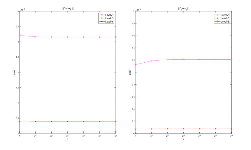
In the computation, we take , , , and , respectively. The numerical results by the WG elements are provided in Tables 2 - 5, whereas the numerical outcomes by the WG elements are illustrated in Figure 2.
Tables 2 - 5 demonstrate that optimal convergence rate is achieved in all cases, and the error and the convergence rate are independent of the parameter . To further illustrate the locking-free property of the WG numerical scheme, we plot the errors in various norms by the WG elements under different parameter values in Figure 2. Our numerical results reveal that there are no significant differences among the displacement errors in various norms under different parameter values , showing that the WG scheme remains unaffected by the parameter , thus validating its locking-free characteristic.
| Level | order | order | ||
|---|---|---|---|---|
| 2 | 8.4869e+00 | – | 7.3595e-01 | – |
| 3 | 3.4276e+00 | 1.3080 | 1.6826e-01 | 2.1289 |
| 4 | 1.3982e+00 | 1.2937 | 3.9187e-02 | 2.1022 |
| 5 | 6.3134e-01 | 1.1471 | 9.5265e-03 | 2.0404 |
| 6 | 3.0518e-01 | 1.0488 | 2.3620e-03 | 2.0120 |
| 7 | 1.5117e-01 | 1.0135 | 5.8919e-04 | 2.0032 |
| Level | order | order | ||
|---|---|---|---|---|
| 2 | 8.5356e+00 | – | 7.2393e-01 | – |
| 3 | 3.4411e+00 | 1.3106 | 1.6342e-01 | 2.1472 |
| 4 | 1.3952e+00 | 1.3024 | 3.7740e-02 | 2.1145 |
| 5 | 6.2668e-01 | 1.1547 | 9.1410e-03 | 2.0457 |
| 6 | 3.0226e-01 | 1.0519 | 2.2638e-03 | 2.0136 |
| 7 | 1.4963e-01 | 1.0144 | 5.6451e-04 | 2.0036 |
| Level | order | order | ||
|---|---|---|---|---|
| 2 | 8.5375e+00 | – | 7.2370e-01 | – |
| 3 | 3.4418e+00 | 1.3107 | 1.6334e-01 | 2.1475 |
| 4 | 1.3954e+00 | 1.3025 | 3.7716e-02 | 2.1146 |
| 5 | 6.2671e-01 | 1.1548 | 9.1348e-03 | 2.0457 |
| 6 | 3.0227e-01 | 1.0520 | 2.2622e-03 | 2.0137 |
| 7 | 1.4963e-01 | 1.0144 | 5.6413e-04 | 2.0036 |
| Level | order | order | ||
|---|---|---|---|---|
| 2 | 8.5375e+00 | – | 7.2370e-01 | – |
| 3 | 3.4418e+00 | 1.3107 | 1.6334e-01 | 2.1475 |
| 4 | 1.3954e+00 | 1.3025 | 3.7716e-02 | 2.1146 |
| 5 | 6.2671e-01 | 1.1548 | 9.1348e-03 | 2.0457 |
| 6 | 3.0227e-01 | 1.0520 | 2.2622e-03 | 2.0137 |
| 7 | 1.4963e-01 | 1.0144 | 5.6402e-04 | 2.0039 |
Example 5.3.
(Locking-free test with unbounded ) To better demonstrate the robustness of the WG Algorithm 1, we consider the case of unbounded in the following example. Besides, we introduce the standard WG scheme as Algorithm 2 for comparison.
A standard WG scheme for weak formulation (3) is given by finding with on such that
| (67) |
| Robust WG Algorithm 1 | Standard WG Algorithm 2 | |||||||
| Level | order | order | order | order | ||||
| 2 | 1.0388e+00 | – | 6.7609e-02 | – | 1.9489e+00 | – | 1.3797e-01 | – |
| 3 | 4.8696e-01 | 1.0930 | 1.6014e-02 | 2.0779 | 6.6479e-01 | 1.5517 | 2.3331e-02 | 2.5641 |
| 4 | 2.3457e-01 | 1.0538 | 3.9062e-03 | 2.0355 | 2.6238e-01 | 1.3412 | 4.4972e-03 | 2.3752 |
| 5 | 1.1580e-01 | 1.0185 | 9.6880e-04 | 2.0115 | 1.1958e-01 | 1.1336 | 1.0097e-03 | 2.1552 |
| 6 | 5.7689e-02 | 1.0052 | 2.4166e-04 | 2.0032 | 5.8176e-02 | 1.0395 | 2.4431e-04 | 2.0471 |
| 2 | 1.0121e+00 | – | 4.0674e-02 | – | 6.1276e+01 | – | 4.2550e+00 | – |
| 3 | 4.8052e-01 | 1.0748 | 7.4022e-03 | 2.4581 | 1.6791e+01 | 1.8676 | 5.8763e-01 | 2.8562 |
| 4 | 2.3221e-01 | 1.0491 | 1.6058e-03 | 2.2046 | 4.3478e+00 | 1.9494 | 7.6391e-02 | 2.9434 |
| 5 | 1.1470e-01 | 1.0176 | 3.8405e-04 | 2.0639 | 1.1060e+00 | 1.9750 | 9.7094e-03 | 2.9760 |
| 6 | 5.7151e-02 | 1.0050 | 9.4883e-05 | 2.0171 | 2.8240e-01 | 1.9695 | 1.2250e-03 | 2.9866 |
| 2 | 1.0121e+00 | – | 4.0387e-02 | – | 6.0245e+03 | – | 4.1843e+02 | – |
| 3 | 4.8052e-01 | 1.0747 | 7.3213e-03 | 2.4637 | 1.6499e+03 | 1.8685 | 5.7752e+01 | 2.8570 |
| 4 | 2.3221e-01 | 1.0491 | 1.5889e-03 | 2.2040 | 4.2666e+02 | 1.9512 | 7.5044e+00 | 2.9441 |
| 5 | 1.1470e-01 | 1.0176 | 3.8029e-04 | 2.0629 | 1.0808e+02 | 1.9809 | 9.5315e-01 | 2.9770 |
| 6 | 5.7151e-02 | 1.0050 | 9.3978e-05 | 2.0167 | 2.7172e+01 | 1.9919 | 1.1998e-01 | 2.9899 |
| 2 | 1.0121e+00 | – | 4.0384e-02 | – | 6.0235e+05 | – | 4.1836e+04 | – |
| 3 | 4.8052e-01 | 1.0747 | 7.3206e-03 | 2.4638 | 1.6496e+05 | 1.8685 | 5.7742e+03 | 2.8570 |
| 4 | 2.3221e-01 | 1.0491 | 1.5888e-03 | 2.2040 | 4.2658e+04 | 1.9512 | 7.5030e+02 | 2.9441 |
| 5 | 1.1470e-01 | 1.0176 | 3.8026e-04 | 2.0629 | 1.0806e+04 | 1.9809 | 9.5298e+01 | 2.9770 |
| 6 | 5.7151e-02 | 1.0050 | 9.3970e-05 | 2.0167 | 2.7167e+03 | 1.9919 | 1.1996e+01 | 2.9899 |
| Robust WG Algorithm 1 | Standard WG Algorithm 2 | |||||||
| Level | order | order | order | order | ||||
| 2 | 1.7563e-01 | – | 1.1594e-02 | – | 2.2323e-01 | – | 1.6555e-02 | – |
| 3 | 4.6492e-02 | 1.9175 | 1.4888e-03 | 2.9612 | 4.9644e-02 | 2.1688 | 1.6706e-03 | 3.3088 |
| 4 | 1.1873e-02 | 1.9694 | 1.8790e-04 | 2.9862 | 1.2070e-02 | 2.0401 | 1.9386e-04 | 3.1073 |
| 5 | 2.9928e-03 | 1.9881 | 2.3573e-05 | 2.9947 | 3.0051e-03 | 2.0060 | 2.3762e-05 | 3.0283 |
| 6 | 7.5080e-04 | 1.9950 | 2.9511e-06 | 2.9978 | 7.5157e-04 | 1.9994 | 2.9570e-06 | 3.0064 |
| 2 | 1.7665e-01 | – | 1.1347e-02 | – | 5.4862e+00 | – | 4.3735e-01 | – |
| 3 | 4.7125e-02 | 1.9064 | 1.4510e-03 | 2.9671 | 7.1692e-01 | 2.9359 | 2.8535e-02 | 3.9380 |
| 4 | 1.2061e-02 | 1.9662 | 1.8283e-04 | 2.9885 | 9.1586e-02 | 2.9686 | 1.8167e-03 | 3.9733 |
| 5 | 3.0425e-03 | 1.9870 | 2.2925e-05 | 2.9955 | 1.1818e-02 | 2.9541 | 1.1592e-04 | 3.9701 |
| 6 | 7.6349e-04 | 1.9946 | 2.8695e-06 | 2.9981 | 1.6224e-03 | 2.8648 | 7.6768e-06 | 3.9165 |
| 2 | 1.7670e-01 | – | 1.1347e-02 | – | 5.3982e+02 | – | 4.2981e+01 | – |
| 3 | 4.7144e-02 | 1.9061 | 1.4506e-03 | 2.9676 | 7.0482e+01 | 2.9371 | 2.8029e+00 | 3.9387 |
| 4 | 1.2066e-02 | 1.9661 | 1.8275e-04 | 2.9887 | 8.9481e+00 | 2.9776 | 1.7782e-01 | 3.9784 |
| 5 | 3.0438e-03 | 1.9870 | 2.2914e-05 | 2.9956 | 1.1257e+00 | 2.9907 | 1.1180e-02 | 3.9914 |
| 6 | 7.6382e-04 | 1.9946 | 2.8680e-06 | 2.9981 | 1.4113e-01 | 2.9958 | 7.0060e-04 | 3.9962 |
| 2 | 1.7670e-01 | – | 1.1347e-02 | – | 5.3973e+04 | – | 4.2974e+03 | – |
| 3 | 4.7144e-02 | 1.9061 | 1.4506e-03 | 2.9676 | 7.0471e+03 | 2.9371 | 2.8025e+02 | 3.9387 |
| 4 | 1.2066e-02 | 1.9661 | 1.8275e-04 | 2.9887 | 8.9468e+02 | 2.9776 | 1.7779e+01 | 3.9784 |
| 5 | 3.0439e-03 | 1.9870 | 2.2914e-05 | 2.9955 | 1.1256e+02 | 2.9907 | 1.1178e+00 | 3.9914 |
| 6 | 7.6387e-04 | 1.9945 | 2.8687e-06 | 2.9978 | 1.4110e+01 | 2.9958 | 7.0048e-02 | 3.9962 |
In the computation, we repeat the computational procedure for various parameter values with . The obtained numerical results are presented in Tables 6 -7. In the case of and WG elements, it is observed that the displacement errors resulting from the standard WG Algorithm 2 exhibit an increasing trend as the parameter is incremented. However, the WG Algorithm 1 shows a distinctive characteristic: the displacement errors remain unaffected by variations in the constant . This finding signifies the robustness of the WG Algorithm 1 with respect to the constant .
Acknowledgments
Y. Wang was supported by the the National Natural Science Foundation of China (grant No. 12171244). R. Zhang and R. Wang were supported by the National Natural Science Foundation of China (grant No. 11971198, 12001230), the National Key Research and Development Program of China (grant No. 2020YFA0713602), and the Key Laboratory of Symbolic Computation and Knowledge Engineering of Ministry of Education of China
References
- [1] S. Adams and B. Cockburn, A mixed finite element method for elasticity in three dimensions, J. Sci. Comput., 25 (2005), pp. 515–521.
- [2] E. Artioli, S. de Miranda, C. Lovadina, and L. Patruno, A family of virtual element methods for plane elasticity problems based on the Hellinger-Reissner principle, Comput. Methods Appl. Mech. Engrg., 340 (2018), pp. 978–999.
- [3] I. Babuška and M. Suri, On locking and robustness in the finite element method, SIAM J. Numer. Anal., 29 (1992), pp. 1261–1293.
- [4] L. Beirão da Veiga, F. Brezzi, and L. D. Marini, Virtual elements for linear elasticity problems, SIAM J. Numer. Anal., 51 (2013), pp. 794–812.
- [5] S. C. Brenner and L. R. Scott, The mathematical theory of finite element methods. Texts in Applied Mathematics, vol. 15, Springer, New York, 3rd ed., 2008.
- [6] S. C. Brenner and L.-Y. Sung, Linear finite element methods for planar linear elasticity, Math. Comp., 59 (1992), pp. 321–338.
- [7] F. Brezzi and M. Fortin, Mixed and hybrid finite element methods, Springer, Berlin, 1991.
- [8] C. Carstensen and H. Rabus, The adaptive nonconforming FEM for the pure displacement problem in linear elasticity is optimal and robust, SIAM J. Numer. Anal., 50 (2012), pp. 1264–1283.
- [9] G. Chen and X. Xie, A robust weak Galerkin finite element method for linear elasticity with strong symmetric stresses, Comput. Methods Appl. Math., 16 (2016), pp. 389–408.
- [10] L. Chen, J. Hu, and X. Huang, Fast auxiliary space preconditioners for linear elasticity in mixed form, Math. Comp., 87 (2018), pp. 1601–1633.
- [11] W. Chen, F. Wang, and Y. Wang, Weak Galerkin method for the coupled Darcy-Stokes flow, IMA J. Numer. Anal., 36 (2016), pp. 897–921.
- [12] P. G. Ciarlet, Mathematical Elasticity: Three-Dimensional Elasticity, Society for Industrial and Applied Mathematics, Philadelphia, PA, 2021.
- [13] A. Ern and J.-L. Guermond, Finite Elements I: Approximation and Interpolation, Springer, Cham, 2021.
- [14] A. L. Gain, C. Talischi, and G. H. Paulino, On the virtual element method for three-dimensional linear elasticity problems on arbitrary polyhedral meshes, Comput. Methods Appl. Mech. Engrg., 282 (2014), pp. 132–160.
- [15] P. Hansbo and M. G. Larson, Discontinuous Galerkin methods for incompressible and nearly incompressible elasticity by Nitsche’s method, Comput. Methods Appl. Mech. Engrg., 191 (2002), pp. 1895–1908.
- [16] G. Harper, J. Liu, S. Tavener, and B. Zheng, Lowest-order weak Galerkin finite element methods for linear elasticity on rectangular and brick meshes, J. Sci. Comput., 78 (2019), pp. 1917–1941.
- [17] G. B. Harper, Weak Galerkin Finite Element Methods for Elasticity and Coupled Flow Problems, ProQuest LLC, Ann Arbor, MI, 2020. Thesis (Ph.D.)–Colorado State University.
- [18] J. Hu, A new family of efficient conforming mixed finite elements on both rectangular and cuboid meshes for linear elasticity in the symmetric formulation, SIAM J. Numer. Anal., 53 (2015), pp. 1438–1463.
- [19] J. Hu and Z.-C. Shi, Lower order rectangular nonconforming mixed finite elements for plane elasticity, SIAM J. Numer. Anal., 46 (2007/08), pp. 88–102.
- [20] X. Hu, L. Mu, and X. Ye, A weak Galerkin finite element method for the Navier-Stokes equations, J. Comput. Appl. Math., 362 (2019), pp. 614–625.
- [21] F. Huo, R. Wang, Y. Wang, and R. Zhang, A locking-free weak galerkin finite element method for linear elasticity problems, 2023.
- [22] J. Jia, Y.-J. Lee, Y. Feng, Z. Wang, and Z. Zhao, Hybridized weak Galerkin finite element methods for Brinkman equations, Electron. Res. Arch., 29 (2021), pp. 2489–2516.
- [23] C.-O. Lee, J. Lee, and D. Sheen, A locking-free nonconforming finite element method for planar linear elasticity, Adv. Comput. Math., 19 (2003), pp. 277–291.
- [24] Y. Liu and J. Wang, A locking-free finite element method for linear elasticity equations on polytopal partitions, IMA J. Numer. Anal., 42 (2022), pp. 3464–3498.
- [25] L. Mu, Weak Galerkin based a posteriori error estimates for second order elliptic interface problems on polygonal meshes, J. Comput. Appl. Math., 361 (2019), pp. 413–425.
- [26] , A uniformly robust weak Galerkin finite element methods for Brinkman problems, SIAM J. Numer. Anal., 58 (2020), pp. 1422–1439.
- [27] L. Mu, J. Wang, Y. Wang, and X. Ye, A weak Galerkin mixed finite element method for biharmonic equations, in Numerical solution of partial differential equations: theory, algorithms, and their applications, vol. 45 of Springer Proc. Math. Stat., Springer, New York, 2013, pp. 247–277.
- [28] L. Mu, J. Wang, and X. Ye, Weak Galerkin finite element methods for the biharmonic equation on polytopal meshes, Numer. Methods Partial Differential Equations, 30 (2014), pp. 1003–1029.
- [29] L. Mu, J. Wang, X. Ye, and S. Zhang, A weak Galerkin finite element method for the Maxwell equations, J. Sci. Comput., 65 (2015), pp. 363–386.
- [30] L. Mu, X. Ye, and S. Zhang, A stabilizer-free, pressure-robust, and superconvergence weak Galerkin finite element method for the Stokes equations on polytopal mesh, SIAM J. Sci. Comput., 43 (2021), pp. A2614–A2637.
- [31] H. Peng, Q. Zhai, R. Zhang, and S. Zhang, Weak Galerkin and continuous Galerkin coupled finite element methods for the Stokes-Darcy interface problem, Commun. Comput. Phys., 28 (2020), pp. 1147–1175.
- [32] D. Shi and C. Xu, An anisotropic locking-free nonconforming triangular finite element method for planar linear elasticity problem, J. Comput. Math., 30 (2012), pp. 124–138.
- [33] S. Shields, J. Li, and E. A. Machorro, Weak Galerkin methods for time-dependent Maxwell’s equations, Comput. Math. Appl., 74 (2017), pp. 2106–2124.
- [34] L.-n. Sun, Y. Feng, Y. Liu, and R. Zhang, The modified weak Galerkin finite element method for solving Brinkman equations, J. Math. Res. Appl., 39 (2019), pp. 657–676.
- [35] B. Wang and L. Mu, Viscosity robust weak Galerkin finite element methods for Stokes problems, Electron. Res. Arch., 29 (2021), pp. 1881–1895.
- [36] C. Wang, New discretization schemes for time-harmonic Maxwell equations by weak Galerkin finite element methods, J. Comput. Appl. Math., 341 (2018), pp. 127–143.
- [37] C. Wang, J. Wang, R. Wang, and R. Zhang, A locking-free weak Galerkin finite element method for elasticity problems in the primal formulation, J. Comput. Appl. Math., 307 (2016), pp. 346–366.
- [38] J. Wang and X. Ye, A weak Galerkin finite element method for second-order elliptic problems, J. Comput. Appl. Math., 241 (2013), pp. 103–115.
- [39] , A weak Galerkin mixed finite element method for second order elliptic problems, Math. Comp., 83 (2014), pp. 2101–2126.
- [40] , A weak Galerkin finite element method for the stokes equations, Adv. Comput. Math., 42 (2016), pp. 155–174.
- [41] R. Wang, Z. Wang, and J. Liu, Penalty-free any-order weak Galerkin FEMs for linear elasticity on quadrilateral meshes, J. Sci. Comput., 95 (2023), pp. Paper No. 20, 22.
- [42] R. Wang and R. Zhang, A weak Galerkin finite element method for the linear elasticity problem in mixed form, J. Comput. Math., 36 (2018), pp. 469–491.
- [43] T. P. Wihler, Locking-free adaptive discontinuous Galerkin FEM for linear elasticity problems, Math. Comp., 75 (2006), pp. 1087–1102.
- [44] S.-Y. Yi, A lowest-order weak Galerkin method for linear elasticity, J. Comput. Appl. Math., 350 (2019), pp. 286–298.
- [45] Q. Zhai, H. Xie, R. Zhang, and Z. Zhang, The weak Galerkin method for elliptic eigenvalue problems, Commun. Comput. Phys., 26 (2019), pp. 160–191.
- [46] Q. Zhai and R. Zhang, Lower and upper bounds of Laplacian eigenvalue problem by weak Galerkin method on triangular meshes, Discrete Contin. Dyn. Syst. Ser. B, 24 (2019), pp. 403–413.
- [47] J. Zhang, K. Zhang, J. Li, and X. Wang, A weak Galerkin finite element method for the Navier-Stokes equations, Commun. Comput. Phys., 23 (2018), pp. 706–746.
- [48] R. Zhang and Q. Zhai, A weak Galerkin finite element scheme for the biharmonic equations by using polynomials of reduced order, J. Sci. Comput., 64 (2015), pp. 559–585.
- [49] T. Zhang and T. Lin, An analysis of a weak Galerkin finite element method for stationary Navier-Stokes problems, J. Comput. Appl. Math., 362 (2019), pp. 484–497.
- [50] Y. Zhang, A weak Galerkin mixed finite element method for linear elasticity equations, ProQuest LLC, Ann Arbor, MI, 2015. Thesis (Ph.D.)–Oklahoma State University.