White-Box Transformers via Sparse Rate Reduction:
Compression Is All There Is?

Abstract

In this paper, we contend that a natural objective of representation learning is to compress and transform the distribution of the data, say sets of tokens, towards a low-dimensional Gaussian mixture supported on incoherent subspaces. The goodness of such a representation can be evaluated by a principled measure, called sparse rate reduction, that simultaneously maximizes the intrinsic information gain and extrinsic sparsity of the learned representation. From this perspective, popular deep network architectures, including transformers, can be viewed as realizing iterative schemes to optimize this measure. Particularly, we derive a transformer block from alternating optimization on parts of this objective: the multi-head self-attention operator compresses the representation by implementing an approximate gradient descent step on the coding rate of the features, and the subsequent multi-layer perceptron sparsifies the features. This leads to a family of white-box transformer-like deep network architectures, named crate, which are mathematically fully interpretable. We show, by way of a novel connection between denoising and compression, that the inverse to the aforementioned compressive encoding can be realized by the same class of crate architectures. Thus, the so-derived white-box architectures are universal to both encoders and decoders. Experiments show that these networks, despite their simplicity, indeed learn to compress and sparsify representations of large-scale real-world image and text datasets, and achieve performance very close to highly engineered transformer-based models: ViT, MAE, DINO, BERT, and GPT2. We believe the proposed computational framework demonstrates great potential in bridging the gap between theory and practice of deep learning, from a unified perspective of data compression. Code is available at: https://ma-lab-berkeley.github.io/CRATE.

1 Introduction

1.1 The Representation Learning Problem

In recent years, deep learning has seen tremendous empirical success in processing and modeling massive amounts of high-dimensional and multi-modal data (Krizhevsky et al., 2009; He et al., 2016; Radford et al., 2021; Chen et al., 2020; He et al., 2022). As argued by Ma et al. (2022), much of this success is owed to deep networks’ ability in effectively learning compressible low-dimensional structures in the data distribution and then transforming the distribution to a parsimonious, i.e. compact and structured, representation. Such a representation then facilitates many downstream tasks, e.g., in vision, classification (He et al., 2016; Dosovitskiy et al., 2021), recognition and segmentation (Carion et al., 2020; He et al., 2020; Kirillov et al., 2023), and generation (Karras et al., 2019; Rombach et al., 2022; Saharia et al., 2022).

Representation learning via compressive encoding and decoding.

To state the common problem behind all these practices more formally, one may view a given dataset as samples of a random vector $\bm{x}$ in a high-dimensional space, say $\mathbb{R}^{D}$. Typically, the distribution of $\bm{x}$ has much lower intrinsic dimension than the ambient space. Generally speaking, by learning a representation, we typically mean to learn a continuous mapping, say $f(\cdot)$, that transforms $\bm{x}$ to a so-called feature vector $\bm{z}$ in another (typically lower-dimensional) space, say $\mathbb{R}^{d}$. It is hopeful that through such a mapping:

$$\bm{x}\in\mathbb{R}^{D}\xrightarrow{\hskip 5.69054ptf(\bm{x})\hskip 5.69054pt}\bm{z}\in\mathbb{R}^{d},$$ (1)

the low-dimensional intrinsic structures of $\bm{x}$ are identified and represented by $\bm{z}$ in a more compact and structured way so as to facilitate subsequent tasks such as classification or generation. The feature $\bm{z}$ can be viewed as a (learned) compact code for the original data $\bm{x}$, so the mapping $f$ is also called an encoder. The fundamental question of representation learning, then, and a central problem that we will address in this work, is:

What is a principled and effective measure for the goodness of representations?

Conceptually, the quality of a representation $\bm{z}$ depends on how well it identifies the most relevant and sufficient information of $\bm{x}$ for subsequent tasks, and how efficiently it represents this information. For long it was believed and argued that “sufficiency” or “goodness” of a learned feature should be defined in terms of a specific task. For example, $\bm{z}$ just needs to be sufficient for predicting a class label $\bm{y}$ in a classification problem. To understand the role of deep learning or deep networks in this type of representation learning, Tishby and Zaslavsky (2015) proposed the information bottleneck framework, which suggests that a measure of feature goodness is to maximize the mutual information between $\bm{z}$ and $\bm{y}$ while minimizing the mutual information between $\bm{z}$ and $\bm{x}$.

Nevertheless, in recent years the predominant practice has been to learn first a task-agnostic representation by pre-training a large deep neural network, in some cases known as a foundation model (Bommasani et al., 2021). The so-learned representation can subsequently be fine-tuned for multiple specific tasks. This has been shown to be more effective and efficient for many practical tasks across diverse data modalities, including speech (Radford et al., 2023), language (Brown et al., 2020), and natural images (Oquab et al., 2023). Notice that representation learning in this context is very different from that for a specific task, where $\bm{z}$ only needs to be good enough for predicting a specific $\bm{y}$. In a task-agnostic setting, the learned representation $\bm{z}$ needs to encode almost all essential information about the distribution of the data $\bm{x}$. That is, the learned representation $\bm{z}$ not only is a more compact and structured representation for the intrinsic structures of $\bm{x}$, but can also recover $\bm{x}$ to a certain degree of faithfulness. Hence, it is natural to ask, in the task-agnostic context, what a principled measure of goodness for a learned (feature) representation should be.

Conceptually, we argue that one effective way, perhaps the only way, to verify whether a representation $\bm{z}$ has encoded sufficient information about $\bm{x}$ is to see how well we can recover $\bm{x}$ from $\bm{z}$ through an (inverse) mapping, say $g$, known as a decoder (or a generator):

$$\bm{x}\in\mathbb{R}^{D}\xrightarrow{\hskip 5.69054ptf(\bm{x})\hskip 5.69054pt}\bm{z}\in\mathbb{R}^{d}\xrightarrow{\hskip 5.69054ptg(\bm{z})\hskip 5.69054pt}\widehat{\bm{x}}\in\mathbb{R}^{D}.$$ (2)

As the encoder $f$ is typically compressive and lossy, we should not expect the inverse mapping to recover $\bm{x}$ exactly, but an approximate $\widehat{\bm{x}}=g\circ f(\bm{x})\approx\bm{x}$. We normally seek optimal encoding and decoding mappings such that the decoded $\widehat{\bm{x}}$ is the closest to $\bm{x}$, either sample-wise—say, by minimizing the expected mean squared error—or in a relaxed distributional sense. We refer to the above process as compressive encoding and decoding or compressive autoencoding. This idea is highly compatible with the original goals laid out for autoencoders by Kramer (1991); Hinton and Zemel (1993), which can be viewed as a generalization of the classic principal component analysis (Jolliffe, 2002) for the case where the low-dimensional structure of $\bm{x}$ is linear.

Through tremendous empirical efforts over the last eleven years, it has become clear that deep networks are very effective in modeling nonlinear encoding and decoding mappings. Almost all applications of deep learning, including those mentioned above, rely on realizing such an encoding or decoding scheme partially or entirely by learning $f$ or $g$ separately or together. Although, conceptually, the decoder $g$ should be the “inverse” to the encoder $f$, in practice it has never been clear how the architectures of encoder and decoder should be related to each other. In many case, the architectural design of the decoder has little to do with that of the encoder, often chosen via empirical tests and ablations (e.g., in masked autoencoders (He et al., 2021)). We believe a good theoretical framework for representation learning should clearly reveal relationships between architectures for the encoder and the decoder. We strive to achieve this level of clarity in this work.

1.2 Review of Existing Approaches

Opening the black-box of modern deep networks through compression.

Along the development of deep learning, many deep network architectures have been proposed and practiced for $f$ or $g$, from the classic LeNet (LeCun et al., 1998) to AlexNet (Krizhevsky et al., 2012), to ResNet (He et al., 2016) and then to the more recent transformer (Vaswani et al., 2017). Despite their popularity, these networks have largely been designed empirically and trained and used as “black-box” function approximators. As a result, desired properties of the learned feature representation $\bm{z}$ are not clearly specified or justified, and many heuristic measures or loss functions have been proposed and practiced for training task-agnostic representations with these models.

Figure 1: Deep network layers $f^{\ell}$ which optimize the rate reduction. The separate components of the data distribution are transformed by the network operators to a configuration which maximizes the information gain. Here, $f$ may be realized by a ReduNet (Chan et al., 2022), in which each layer implements a gradient descent iteration for optimizing the rate reduction.

The recent work of Yu et al. (2020); Chan et al. (2022) has attempted to provide a principled framework that interprets the deep architectures of the ResNet and CNNs from the perspective of optimizing a measure of “information gain” for the learned representation. When the structured representation sought is a mixture of low-dimensional Gaussians, the information gain can be precisely measured by the so-called coding rate reduction, denoted as $\Delta R(\bm{z})$, and defined as the difference between the coding rates for the feature set as a whole and the coding rate for its structured components. It was shown that one can derive from this objective a deep network architecture, known as the ReduNet (Yu et al., 2020; Chan et al., 2022), that shares a striking resemblance to ResNets and CNNs. The layers of a ReduNet are fully interpretable as realizing an iterative gradient descent method for optimizing the coding rate reduction objective $\Delta R(\bm{z})$, as in Figure 1:

$$f\colon\bm{x}\xrightarrow{\hskip 2.84526ptf^{\mathrm{pre}}\hskip 2.84526pt}\bm{z}^{1}\rightarrow\cdots\rightarrow\bm{z}^{\ell}\xrightarrow{\hskip 2.84526ptf^{\ell}\hskip 2.84526pt}\bm{z}^{\ell+1}\rightarrow\cdots\xrightarrow{\hskip 2.84526ptf^{L}\hskip 2.84526pt}\bm{z}^{L+1}=\bm{z},$$ (3)

where $f^{\mathrm{pre}}$ is some data pre-processing map, and

$$\bm{z}^{\ell+1}=f^{\ell}(\bm{z}^{\ell})\approx\bm{z}^{\ell}+\eta\nabla\big{[}\Delta R(\bm{z}^{\ell})\big{]}$$ (4)

i.e., each layer $\ell$ is constructed to incrementally optimize the $\Delta R(\bm{z}^{\ell})$ by taking an approximate gradient ascent step with step size $\eta$. We will refer to such a mathematically interpretable network as a “white-box” deep network in the sense that the motivation and structure of each network layer is well understood (i.e., as approximating an incremental improvement of some desired objective function). Although rate reduction offers a good theoretical framework for understanding architectures of existing deep networks such as ResNets and CNNs, direct implementations of ReduNet have not yet generated competitive practical performance on real-world datasets and tasks at scale. In this work, we will see how this outstanding gap between theory and practice can be bridged through a generalization and improvement to the rate reduction objective such that its gradient descent operator resembles the structure of a transformer layer, in such a way that the resulting trasnformer-like architecture achieves competitive empirical performance.

Transformer models and compression.

In recent years, transformers (Vaswani et al., 2017) have emerged as the most popular, nearly universal, model of choice for the encoder $f$ and decoder $g$ in learning representations for high-dimensional structured data, such as text (Vaswani et al., 2017; Devlin et al., 2019; Brown et al., 2020), images (Dosovitskiy et al., 2021; Dehghani et al., 2023), and other types of signals (Gong et al., 2023; Arnab et al., 2021). In a nutshell, a transformer first converts each data point (such as a text corpus or image) into a set or sequence of tokens, and then performs further processing on the token sets, in a medium-agnostic manner (Vaswani et al., 2017; Dosovitskiy et al., 2021). A cornerstone of the transformer model is the so-called (self-)attention layer, which exploits the statistical correlations among the sequence of tokens to refine the token representation. Yet the transformer network architecture is empirically designed and lacks a rigorous mathematical interpretation. In fact, the output of the attention layer itself has several competing interpretations (Vidal, 2022; Li et al., 2023a). As a result, the statistical and geometric relationship between the data $\bm{x}$ and the final representation $\bm{z}$ learned by a transformer largely remains a mysterious black box.

Nevertheless, in practice, transformers have been highly successful in learning compact representations that perform well on many downstream tasks. In particular, it serves as the backbone architecture for the celebrated large language models (LLMs) such as OpenAI’s GPT-4 (OpenAI, 2023b). Although the precise reason why it works well remains unclear, it has been hypothesized by OpenAI’s researchers from a heuristic standpoint that the transformer architecture in LLMs implicitly minimizes the Kolmogorov complexity of the representations (Simons Institute, 2023), a quantitative notion of compression measured by the length of the code that can generate the data in consideration. However, we know that Kolmogorov complexity is largely a theoretical concept and in general not computationally tractable for high-dimensional distributions. Hence, if transformers in LLMs indeed conduct compression, they should be based on a measure of complexity that is amenable to tractable and efficient computation. The design of Helmholtz machines (and Boltzman machines) based on the minimum description length principle can be viewed as early attempts to make compression computable (Hinton and Zemel, 1993). In this work, we argue that a natural choice of this computable measure of compression behind transformers is precisely a combination of rate reduction and sparsity of the learned representations. As we will see, revealing such a measure could be the key to understand the transformer architecture.

Denoising-diffusion models and compression.

Diffusion models (Sohl-Dickstein et al., 2015; Ho et al., 2020; Song and Ermon, 2019; Song et al., 2021b, a) have recently become a popular method for learning high-dimensional data distributions, particularly of natural images, which are known to be highly structured in a manner that is notoriously difficult to model mathematically (Ruderman, 1994; Wakin et al., 2005; Donoho and Grimes, 2005). The core concept of diffusion models is to start with features $\bm{z}$ sampled from a Gaussian noise distribution (or some other standard template) and denoise and deform the feature distribution until it converges to the original data distribution, which often has low intrinsic dimension. This process is computationally intractable if modeled in just one step (Koehler et al., 2023), so it is typically broken into multiple incremental steps that denoise iteratively, as in Figure 2:

$$g\colon\bm{z}=\widetilde{\bm{z}}^{0}\rightarrow\widetilde{\bm{z}}^{1}\rightarrow\cdots\rightarrow\widetilde{\bm{z}}^{\ell}\xrightarrow{\hskip 2.84526ptg^{\ell}\hskip 2.84526pt}\widetilde{\bm{z}}^{\ell+1}\rightarrow\cdots\rightarrow\widetilde{\bm{z}}^{L}\xrightarrow{\hskip 2.84526ptg^{\mathrm{post}}\hskip 2.84526pt}\widehat{\bm{x}},$$ (5)

where $g^{\mathrm{post}}$ is a data post-processing map, and

$$\widetilde{\bm{z}}^{\ell+1}=g^{\ell}(\widetilde{\bm{z}}^{\ell})=\widetilde{\bm{z}}^{\ell}+\tau\nabla\log q^{\ell}(\widetilde{\bm{z}}^{\ell}),$$ (6)

where $q^{\ell}$ is the density of $\widetilde{\bm{z}}^{\ell}$, i.e., the density of $\widetilde{\bm{z}}^{L}$ after corruption with the $\ell$-th scale of Gaussian noise, and $\nabla\log q^{\ell}$ is the so-called score function (Hyvärinen, 2005), or equivalently an estimate for the “optimal denoising function” for $q^{\ell}$ (Efron, 2011a). In practice, the score function is modeled using a generic black-box deep network. Diffusion models have shown effectiveness at learning and sampling from the data distribution (Karras et al., 2022; Chen et al., 2023a; Rombach et al., 2022). However, despite some recent efforts (Song et al., 2023), they generally do not establish any clear correspondence between the initial features and data samples. Hence, diffusion models themselves do not offer a parsimonious or interpretable representation of the data distribution. Yet, conceptually, the above iterative denoising process (5) is compressing the feature distribution onto a targeted low-dimensional data distribution. In this work, we will show that if one were to compress and transform a distribution onto a standard mixture of (low-dimensional) Gaussians, the associated optimal denoising function takes an explicit form that is similar to the gradient of the rate reduction and to a transformer layer. This provides a path to take a transformer-like encoder $f$ designed to compress the data distribution into a parsimonious and structured representation, and derive its distributional inverse through a process analogous to 5, yielding a white-box architecture for compressive autoencoding.

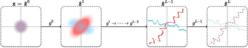
Figure 2: Distribution flow in denoising-diffusion models. Starting with generic noise $\bm{z}=\widetilde{\bm{z}}^{0}$, the probability density of intermediate iterates is shaped towards the true distribution of $\widetilde{\bm{z}}^{L}$ locally and iteratively through the operators $g^{\ell}$, which use the score function $\nabla\log q^{\ell}$ at each layer $\ell$.

Low-dimensionality promoting measures: sparsity and rate reduction.

In both of the previous popular methods, transformers and denoising-diffusion models, a representation was learned implicitly as a byproduct of solving a downstream task (e.g., classification or generation/sampling) using deep networks. The networks used are typically chosen empirically. Therefore, it is difficult to rigorously ensure or impose any desired properties for the learned representation, except by trial and error. However, complementary to these popular empirical practices, a line of research has attempted to explicitly learn a desired representation of the data distribution as a task in and of itself; this is most commonly done by trying to explicitly identify and represent low-dimensional structures in the input data. Classical examples of this paradigm include model-based approaches such as sparse coding (Olshausen and Field, 1997; Chen et al., 2018) and dictionary learning (Aharon et al., 2006; Spielman et al., 2012; Gribonval et al., 2015; Zhai et al., 2020b), out of which grew early attempts at designing and interpreting deep network architectures as learning a sparse representation (Papyan et al., 2018; Bruna and Mallat, 2013). More recent approaches build instead from a model-free perspective, where one learns a representation through a sufficiently-informative pretext task such as compressing similar and separating dissimilar data via contrastive learning (Tian et al., 2020; Wang et al., 2022; Bardes et al., 2022; Shwartz-Ziv and LeCun, 2023). Compared to black-box deep learning approaches, both model-based and model-free representation learning schemes have the advantage of being more interpretable: they allow users to explicitly design desired properties of the learned representation $\bm{z}$. To a large extent, the rate reduction framework (Yu et al., 2020; Chan et al., 2022; Pai et al., 2023) strikes a good balance between the above model-based and model-free methods. Like contrastive learning, it aims to identify the data distribution by compressing similar/correlated data and separating dissimilar/uncorrelated data (Yu et al., 2020). Meanwhile, like the model-based methods, it actively maps the data distribution to a family of desired representations, say a mixture of low-dimensional Gaussians (Ma et al., 2007; Vidal et al., 2016).

Unrolled optimization: a unified paradigm for network interpretation & design.

As we have discussed above, low-dimensionalty promoting measures, such as sparsity or coding rate reduction, allow users to construct white-box deep network architectures (Gregor and LeCun, 2010; Chan et al., 2022) in a forward-construction fashion by unrolling an optimization strategy for the chosen objective of the representations, such that each layer of the constructed network implements an iteration of the optimization algorithm (Gregor and LeCun, 2010; Chan et al., 2022; Tolooshams and Ba, 2022). In his recent work, Hinton (2022) has also begun to hypothesize that the role of a deep network, with its forward pass, is likely to optimize certain feature goodness layer-wise. In this paradigm, the most challenging question is:

What fundamental measure of goodness for the representations is a deep network trying to optimize in its forward pass?

In the unrolled optimization paradigm, if the desired objectives are narrowly defined, say promoting sparsity alone (Papyan et al., 2018; Bruna and Mallat, 2013), it has so far proved difficult to arrive at network architectures that can achieve competitive practical performance on large real-world datasets. Other work has attempted to derive empirically-designed popular network architectures through unrolled optimization on a reverse-engineered learning objective for the representation, such as Yang et al. (2022); Hoover et al. (2023); Weerdt et al. (2023). In this case, the performance of the networks may remain intact, but the reverse-engineered representation learning objective is usually highly complex and not interpretable, and the properties of the optimal representation—or indeed the actually-learned representation—remain opaque. Such approaches do not retain the key desired benefits of unrolled optimization. As we will argue in this work, to measure the goodness of a learned representation in terms of its intrinsic compactness and extrinsic simplicity, it is crucial to combine the measure of sparsity (Papyan et al., 2018; Bruna and Mallat, 2013) and that of coding rate reduction (Yu et al., 2020; Chan et al., 2022). As we will see, this combination will largely resolve the aforementioned limitations of extant methods that rely solely on sparsity or solely on rate reduction.

1.3 Goals and Contributions of This Work

From the above discussion, we can observe that there has been an outstanding wide gap between the practice and theory of representation learning via deep networks. The fast advancement in the practice of deep learning has been primarily driven by empirical black-box models and methods that lack clear mathematical interpretations or rigorous guarantees. Yet almost all existing theoretical frameworks have only attempted to address limited or isolated aspects of practice, or only proposed and studied idealistic models that fall far short of producing practical performance that can compete with their empirical counterparts.

Bridging the gap between theory and practice.

Therefore, the primary goal of this work is to remedy this situation with a more complete and unifying framework that has shown great promise in bridging this gap between theory and practice. On one hand, this new framework is able to provide a unified understanding of the many seemingly disparate approaches and methods based on deep networks, including compressive encoding/decoding (or autoencoding), rate reduction, and denoising-diffusion. On the other hand, as we will see, this framework can guide us to derive or design deep network architectures that are not only mathematically fully interpretable but also obtain competitive performance on almost all learning tasks on large-scale real-world image or text datasets.

A theory of white-box deep networks.

More specifically, we propose a unified objective, a principled measure of goodness, for learning compact and structured representations. For a learned representation, this objective aims to optimize both its intrinsic complexity in terms of coding rate reduction and its extrinsic simplicity in terms of sparsity. We call this objective the sparse rate reduction, specified later in  (15) and (17). The intuition behind this objective is illustrated in Figure 3. To optimize this objective, we propose to learn a sequence of incremental mappings that emulate unrolling certain gradient-descent-like iterative optimization scheme for the objective function. As we will see, this naturally leads to a transformer-like deep network architecture that is entirely a “white box” in the sense that its optimization objective, network operators, and learned representation are all fully interpretable mathematically. We name such a white-box deep architecture “crate,” or “crate-Transformer,” short for a Coding-RATE transformer. We also show mathematically that these incremental mappings are invertible in a distributional sense, and their inverses consist of essentially the same class of mathematical operators. Hence a nearly identical crate architecture can be used for realizing encoders, decoders, or together for auto-encoders.

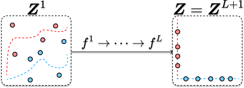
Figure 3: The optima of the sparse rate reduction. After pre-processing input data $\bm{X}$ into a sequence of tokens $\bm{Z}^{1}$, our crate network attempts to optimize the sparse rate reduction of the token features $\bm{Z}=\bm{Z}^{L+1}$. The optimal representations, according to the sparse rate reduction objective, are linearized—having low-dimensional linear subspace structure—sparse—where the subspaces are axis-aligned—and compressed—adhering closely to that structure, with low or no noise. In the sequel, we discuss how crate achieves optimal representations via constructing each layer to iteratively optimize the sparse rate reduction.

Practice of white-box deep networks.

To show that this framework can truly bridge the gap between theory and practice, we have conducted extensive experiments on both image and text data to evaluate the practical performance of the crate model on a wide range of learning tasks and settings that conventional transformers have demonstrated strong performance. Surprisingly, despite its conceptual and structural simplicity, crate has demonstrated competitive performance with respect to its black-box counterparts on all tasks and settings, including image classification via supervised learning (Dosovitskiy et al., 2021), unsupervised masked completion for imagery and language data (He et al., 2022; Devlin et al., 2019; Liu et al., 2019), self-supervised feature learning for imagery data (Caron et al., 2021), and language modeling via next-word prediction (Radford et al., 2018). Moreover, the crate model demonstrates additional practical benefits: each layer and network operator statistically and geometrically meaningful, the learned model is significantly more interpretable compared to black-box transformers, and the features show semantic meaning, i.e., they can be easily used to segment an object from its background and partition it into shared parts.

Note that with limited resources, in this work we do not strive for state-of-the-art performance on all of the aforementioned tasks, which would require heavy engineering or extensive fine-tuning; nor can we implement and test our models at current industrial scales. Overall, our implementations for these tasks are basic and uniform, without significant task-specific customization. Nevertheless, we believe these experiments have convincingly verified that the derived white-box deep network crate model is universally effective and sets a solid baseline for further engineering development and improvement.

Outline of the paper:

• In Section 2.1, we give a formal formulation for representation learning, both conceptually and quantitatively. We argue that a principled measure of goodness for a learned feature representation is the so-called sparse rate reduction that simultaneously characterizes the representation’s intrinsic information gain and its extrinsic sparsity. In Section 2.2, we contend that the fundamental role of a deep network is to optimize such an objective by unrolling an iterative optimization scheme such as gradient descent.

• From Section 2.3 to Section 2.5, we show that a transformer-like deep architecture can be derived from unrolling an alternating minimization scheme for the sparse rate reduction objective. In particular, in Section 2.3 we derive a multi-head self-attention layer as an unrolled gradient descent step to minimize the lossy coding rate of the token set with respect to a (learned) low-dimensional Gaussian mixture codebook. In Section 2.4 we show that the multi-layer perceptron which immediately follows the multi-head self-attention in transformer blocks can be interpreted as (and replaced by) a layer which constructs a sparse coding of the token representations. This creates a new white-box, i.e., fully mathematically interpretable, transformer-like architecture called crate, summarized in Section 2.5, where each layer performs a single step of an alternating minimization algorithm to optimize the sparse rate reduction objective.

• In Section 3 we reveal a fundamental connection between compression via rate reduction and the diffusion-denoising process for learning a representation for the data distribution. In particular, we show that if one denoises the tokens towards a family of low-dimensional subspaces, the associated score function assumes an explicit form similar to a self-attention operator seen in transformers. We also establish that the gradient descent of rate reduction essentially conducts structured denoising against the (learned) low-dimensional Gaussian mixture model for the tokens. This connection allows us to construct a white-box decoder based on a structured diffusion process, as a distributional inverse to the structured denoising process implemented by the crate encoder. One can show that the decoder essentially shares the same architecture as the encoder, and they together form a symmetric white-box autoencoder that is fully mathematically interpretable.

• In Section 4 we provide extensive experimental results to show that the crate networks, despite being simple and often smaller, can already learn the desired compressed and sparse representations on large-scale real-world datasets, all while achieving performance on par with seasoned transformer networks on a wide variety of popular tasks and settings, including ViT for image classification, MAE for image completion, DINO for image segmentation with self-supervised learning, and BERT and GPT for text completion and prediction. In addition, we demonstrate, both qualitatively and quantitatively, that the internal representations of crate are more interpretable than vanilla vision transformers trained on image classification.

At the end of the paper, in Appendices A to C, we provide adequate technical details and experimental details for the above sections, to ensure that all our claims in the main body are verifiable and experiments are reproducible. Appendix D gives PyTorch-like pseudocode for our implementation of crate.

2 White-Box Encoding via Structured Lossy Compression

In this section, we provide a technical formulation and justification for our new framework and approach. To wit, we provide a (gentle yet) complete derivation from first principles of our white-box transformer approach. While being a self-contained introduction to our framework, and providing a transparently interpretable transformer-like deep network architecture, it also foreshadows several connections between previously disparate technical approaches to representation learning. These we make clear in the next Section 3 en route to extending our technical framework to autoencoding.

Notation.

We consider a general learning setup associated with real-world signals. We have some random variable $\bm{X}=\begin{bmatrix}\bm{x}_{1},\dots,\bm{x}_{N}\end{bmatrix}\in\mathbb{R}^{D\times N}$ which is our data source; each $\bm{x}_{i}\in\mathbb{R}^{D}$ is interpreted as a token, there are $N$ tokens $\bm{x}_{i}$ in each data sample $\bm{X}$, and the $\bm{x}_{i}$’s may have arbitrary correlation structures. To obtain a useful representation of the input, we learn an encoder mapping $f\colon\mathbb{R}^{D\times N}\to\mathbb{R}^{d\times n}$. The features—that is, the output of the encoder—are denoted by the random variable $\bm{Z}\doteq f(\bm{X})\doteq\begin{bmatrix}\bm{z}_{1},\dots,\bm{z}_{n}\end{bmatrix}\in\mathbb{R}^{d\times n}$, whence each $\bm{z}_{i}\in\mathbb{R}^{d}$ is a feature vector. The number of features $n$ is typically the same as the number of tokens $N$, or not much more (e.g., due to pre-processing), in which case there is a natural correspondence between feature vectors $\bm{z}_{i}$ and tokens $\bm{x}_{i}$. In the auto-encoding context, we also learn a decoder mapping $g\colon\mathbb{R}^{d\times n}\to\mathbb{R}^{D\times N}$, such that $\bm{X}\approx\widehat{\bm{X}}\doteq g(\bm{Z})\doteq\begin{bmatrix}\widehat{\bm{x}}_{1},\dots,\widehat{\bm{x}}_{N}\end{bmatrix}$, whence each $\widehat{\bm{x}}_{i}\in\mathbb{R}^{D}$ is the auto-encoding of token $\bm{x}_{i}$.

As we have alluded to before, a central question we want to answer in this work is the purpose of such an encoder and decoder in representation learning: namely, how should we design the encoder and decoder mappings to optimize a representation learning objective? As we will see, one specific form of the encoder $f$ and the decoder $g$, that can be naturally deduced through iterative optimization of the objective, is composed of multiple basic operators, also known as layers in the language of deep neural networks. In such cases, we write $f=f^{L}\circ\cdots\circ f^{1}\circ f^{\mathrm{pre}}$ and $g=g^{\mathrm{post}}\circ g^{L-1}\circ\cdots\circ g^{0}$, where $f^{\ell}\colon\mathbb{R}^{d\times n}\to\mathbb{R}^{d\times n}$ and $g^{\ell}\colon\mathbb{R}^{d\times n}\to\mathbb{R}^{d\times n}$ are the $\ell^{\mathrm{th}}$ layer of the encoder and decoder respectively, and $f^{\mathrm{pre}}\colon\mathbb{R}^{D\times N}\to\mathbb{R}^{d\times n}$ and $g^{\mathrm{post}}\colon\mathbb{R}^{d\times n}\to\mathbb{R}^{D\times N}$ are the pre- and post-processing layers respectively. The input to the $\ell^{\mathrm{th}}$ layer of the encoder is denoted $\bm{Z}^{\ell}\doteq\begin{bmatrix}\bm{z}_{1}^{\ell},\dots,\bm{z}_{n}^{\ell}\end{bmatrix}\in\mathbb{R}^{d\times n}$, and the input to the $\ell^{\mathrm{th}}$ layer of the decoder is denoted $\widetilde{\bm{Z}}^{\ell}\doteq\begin{bmatrix}\widetilde{\bm{z}}_{1}^{\ell},\dots,\widetilde{\bm{z}}_{n}^{\ell}\end{bmatrix}\in\mathbb{R}^{d\times n}$. In particular, $\bm{Z}^{\ell+1}=f^{\ell}(\bm{Z}^{\ell})$ and $\widetilde{\bm{Z}}^{\ell+1}=g^{\ell}(\widetilde{\bm{Z}}^{\ell})$. Figure 4 depicts this overall process.

2.1 Desiderata and Objective of Representation Learning

Representation learning via the principle of parsimony and consistency.

Following the framework of rate reduction (Chan et al., 2022), we contend that the goal of representation learning is to find a feature mapping $f\colon\bm{X}\in\mathbb{R}^{D\times N}\to\bm{Z}\in\mathbb{R}^{d\times n}$ which transforms input data $\bm{X}\in\mathbb{R}^{D\times N}$ with a potentially nonlinear and multi-modal distribution to a parsimonious feature representation $\bm{Z}\in\mathbb{R}^{d\times n}$ (Ma et al., 2022). As in Ma et al. (2022), a complete desiderata for the learned representations ought to be:

1. Compressed: being strictly distributed according to some standard low-dimensional structures matching the intrinsic low-dimensionality of the data, so as to ensure a compact encoding of the data.

2. Linearized: the low-dimensional structures have (piecewise) linear geometry, so as to aid interpolation and extrapolation in the representation space.

3. Sparse: the low-dimensional structures corresponding to different parts of the data distribution are statistically incoherent or geometrically orthogonal, and also axis-aligned, so as to ensure a more compact encoding and aid downstream processing.

4. Consistent: for autoencoding/generative purposes, we desire that the learned representation is invertible, in the sense that we can decode features to recover the corresponding input data, either on the level of individual samples or distribution-wise.

For the last item, specifically, we would also like to learn an inverse mapping: $g\colon\bm{Z}\in\mathbb{R}^{d\times n}\to\widehat{\bm{X}}\in\mathbb{R}^{D\times N}$ such that $\widehat{\bm{X}}$ and $\bm{X}$ are quantitatively close in some sense. Figure 4 illustrates the overall process and the desired four goals of such a representation learning. In this section (Section 2), we will mainly show how to achieve the first three items on this list by developing an encoding scheme; we will address the last item in the next section (Section 3) by showing how the proposed encoding scheme can be naturally reversed.

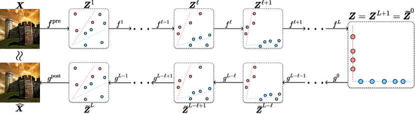
Figure 4: The autoencoding process to be studied in Sections 2 and 3. Each encoder layer $f^{\ell}$ and decoder layer $g^{L-\ell}$ are (partial) inverses of each other. Moreover, the overall representation $\bm{Z}=f(\bm{X})$ is parsimonious (compressed, linearized, and sparse, as in Section 2.1), and the autoencoding is to be consistent in the sense that $\bm{X}\approx\widehat{\bm{X}}$.

An objective which promotes parsimonious representations.

Previously, Yu et al. (2020) have proposed to obtain parsimonious representations via maximizing the information gain (Ma et al., 2022), a principled measure of the information content of the features. A concrete instantiation of the information gain is the coding rate reduction (Yu et al., 2020) of the features, i.e.,

$$\Delta R(\bm{Z}\mid\bm{\Pi}_{[K]})=R(\bm{Z})-R^{c}(\bm{Z}\mid\bm{\Pi}_{[K]}).$$ (7)

The first term $R(\bm{Z})$ in the above expression is an estimate of the lossy coding rate (i.e., rate distortion function) for the whole set of features, when using a codebook adapted to Gaussians. More specifically, if we view the token feature vectors $(\bm{z}_{i})_{i\in[n]}$ in $\bm{Z}\in\mathbb{R}^{d\times n}$ as i.i.d. samples from a single zero-mean Gaussian, an approximation of their (lossy) coding rate, subject to quantization precision $\epsilon>0$, is given in (Ma et al., 2007) as:

$$R(\bm{Z})\doteq\frac{1}{2}\operatorname{logdet}\left(\bm{I}+\alpha\bm{Z}^{\ast}\bm{Z}\right)=\frac{1}{2}\operatorname{logdet}\left(\bm{I}+\alpha\bm{Z}\bm{Z}^{\ast}\right),\quad\text{where}\ \alpha\doteq\frac{d}{n\epsilon^{2}}.$$ (8)

The second term $R^{c}$ in the rate reduction objective (7) is also an estimate of the lossy coding rate, but under a different and more precise codebook—one which views the token feature vectors $(\bm{z}_{i})_{i\in[n]}$ as i.i.d. samples of a mixture of Gaussians, where assignment of tokens to a particular Gaussian is known and specified by the Boolean membership matrices $\bm{\Pi}_{[K]}=(\bm{\Pi}_{k})_{k\in[K]}$, and the $k^{\mathrm{th}}$ Gaussian has $n_{k}$ associated tokens. We obtain an estimate for the coding rate $R^{c}$ as

$$R^{c}(\bm{Z}\mid\bm{\Pi}_{[K]})\doteq\frac{1}{2}\sum_{k=1}^{K}\operatorname{logdet}\left(\bm{I}+\gamma_{k}\bm{Z}\bm{\Pi}_{k}\bm{Z}^{\ast}\right),\quad\text{where}\ \gamma_{k}\doteq\frac{d}{n_{k}\epsilon^{2}}.$$ (9)

As shown in Yu et al. (2020), maximizing the rate reduction $\Delta R$, i.e., the difference between $R$ and $R^{c}$, promotes that the token features $\bm{z}_{i}$ are compactly encoded as a mixture of low-dimensional Gaussian distributions, where different Gaussian are statistically incoherent.

A generalized measure of rate reduction for tokens.

In more realistic and general scenarios, the features $\bm{Z}$ can be a collection of tokens $(\bm{z}_{i})_{i=1}^{N}$ which have a sophisticated and task-specific joint distribution, which can encode rich information about the data which we should also seek to capture in the final representation.

To realize our above desiderata in this context—namely, seeking a compact representation of a complex joint distribution of the token features—we only require that the desired marginal distribution of individual tokens $\bm{z}_{i}$ should be a mixture of (say $K$) low-dimensional Gaussian distributions. Without loss of generality, we may assume that the $k^{\mathrm{th}}$ Gaussian has mean $\mathbf{0}\in\mathbb{R}^{d}$, covariance $\bm{\Sigma}_{k}\succeq\mathbf{0}\in\mathbb{R}^{d\times d}$, and support spanned by the orthonormal basis $\bm{U}_{k}\in\mathbb{R}^{d\times p}$. We denote $\bm{U}_{[K]}=(\bm{U}_{k})_{k=1}^{K}$ to be the set of all bases for the Gaussians. In the sequel, we often identify the basis $\bm{U}_{k}$ with the subspace itself.

For future reference, we provide a formal definition of this statistical model below. Note that we may incorporate random noise as a way to model benign deviations from the previously described idealized model.

Low-Dimensional Gaussian Mixture Codebook:

Let $\bm{Z}=\begin{bmatrix}\bm{z}_{1},\dots,\bm{z}`_{n}\end{bmatrix}\in\mathbb{R}^{d\times n}$ be a matrix-valued random variable. We impose the following statistical model on ${\bm{Z}}$, parameterized by orthonormal bases $\bm{U}_{[K]}=(\bm{U}_{k})_{k\in[K]}\in(\mathbb{R}^{d\times p})^{K}$: each token ${\bm{z}}_{i}$ has marginal distribution given by

$${\bm{z}}_{i}\stackrel{{\scriptstyle d}}{{=}}\bm{U}_{s_{i}}\bm{\alpha}_{i},\quad\forall i\in[n]$$ (10)

where $(s_{i})_{i\in[n]}\in[K]^{n}$ are random variables corresponding to the subspace indices, and $(\bm{\alpha}_{i})_{i\in[n]}\in(\mathbb{R}^{p})^{n}$ are zero-mean Gaussian variables. If we optionally specify a noise parameter $\sigma\geq 0$, we mean that we “diffuse” the tokens with Gaussian noise: by an abuse of notation, each token ${\bm{z}}_{i}$ has marginal distribution given by

$$\bm{z}_{i}\stackrel{{\scriptstyle d}}{{=}}\bm{U}_{s_{i}}\bm{\alpha}_{i}+\sigma\bm{w}_{i},\quad\forall i\in[n]$$ (11)

where $(\bm{w}_{i})_{i\in[n]}\in(\mathbb{R}^{d})^{n}$ are i.i.d. standard Gaussian variables, independent of $s_{i}$ and $\bm{\alpha}_{i}$.

From the perspective of statistics, we may view $\bm{U}_{[K]}$ as multiple “principal subspaces” (Vidal et al., 2016), which, just as in principal component analysis, are preferred to be incoherent or nearly orthogonal to each other. From the perspective of signal processing, we may view $\bm{U}_{[K]}$ as “local signal models” for the input distribution. From the perspective of information theory, we may view the bases $\bm{U}_{[K]}$ as codebooks and the vectors $\bm{\alpha}_{ik}\doteq\bm{U}_{k}^{\ast}\bm{z}_{i}$ as the “codes” of the token features $\bm{z}_{i}$ with respect to these codebooks. Motivated by 10, we desire these codes to have a Gaussian marginal distribution within each subspace; under this model, we can compute the coding rate of these codes, similar to (8), as

$$R(\bm{U}_{k}^{\ast}\bm{Z})\doteq\frac{1}{2}\operatorname{logdet}\left(\bm{I}+\beta(\bm{U}_{k}^{\ast}\bm{Z})^{\ast}(\bm{U}_{k}^{\ast}\bm{Z})\right),\quad\text{where}\ \beta\doteq\frac{p}{n\epsilon^{2}}.$$ (12)

We emphasize that here, under 10, the joint distribution of such $\bm{Z}$ is underspecified, so the true optimal codebook for $\bm{Z}$ is unknown and so the lossy coding rate for $\bm{Z}$ is impossible to compute. However, since the desired marginal distribution of each token $\bm{z}_{i}$ is a mixture of low-dimensional Gaussians supported on subspaces $\bm{U}_{[K]}$, we may obtain an upper bound of the coding rate for the token set $\bm{Z}$, which we denote as $R^{c}$, by projecting the tokens $\bm{z}_{i}$ onto these subspaces and summing up the coding rates on each subspace:

$$R^{c}(\bm{Z}\mid\bm{U}_{[K]})\doteq\sum_{k=1}^{K}R(\bm{U}_{k}^{\ast}\bm{Z})=\frac{1}{2}\sum_{k=1}^{K}\operatorname{logdet}\left(\bm{I}+\beta(\bm{U}_{k}^{\ast}\bm{Z})^{\ast}(\bm{U}_{k}^{\ast}\bm{Z})\right).$$ (13)

This form of the coding rate can be viewed as a generalization to the coding rate $R^{c}$ in the original rate reduction objective defined in 7. In particular, the original objective is defined with respect to a set of known membership labels $\bm{\Pi}_{[K]}$ specific to the particular data realization $\bm{X}$. In contrast, the objective here is defined with respect to subspaces $\bm{U}_{[K]}$ which are in principle defined externally to any specific data realization, though they support the token feature distribution. Since a single token can have nonzero projection onto multiple subspaces $\bm{U}_{k}$, yet must belong to exactly one category defined by $\bm{\Pi}_{k}$, the coding rate defined in 13 may be viewed as a generalization of the coding rate defined in 9. We may correspondingly generalize the coding rate reduction $\Delta R$, obtaining:

$$\Delta R(\bm{Z}\mid\bm{U}_{[K]})\doteq R(\bm{Z})-R^{c}(\bm{Z}\mid\bm{U}_{[K]}).$$ (14)

Sparse rate reduction.

It is easy to see that the rate reduction is invariant to arbitrary joint rotations of the representations and subspaces (Ma et al., 2007). In particular, optimizing the rate reduction may not naturally lead to axis-aligned (i.e., sparse) representations. Therefore, we would like to transform the representations (and their supporting subspaces) so that the features $\bm{Z}$ eventually become sparse with respect to the standard coordinates of the resulting representation space.

The combined rate reduction and sparsification process is illustrated in Figure 3 or Figure 4. Computationally, we may combine the above two goals into a unified objective for optimization:

$$\max_{f\in\mathcal{F}}\mathbb{E}_{\bm{Z}=f(\bm{X})}\big{[}\Delta R(\bm{Z}\mid\bm{U}_{[K]})-\lambda\lVert\bm{Z}\rVert_{0}\big{]},$$ (15)

or equivalently,

$$\max_{f\in\mathcal{F}}\mathbb{E}_{\bm{Z}=f(\bm{X})}\big{[}R(\bm{Z})-{R}^{c}(\bm{Z}\mid\bm{U}_{[K]})-\lambda\lVert\bm{Z}\rVert_{0}\big{]},$$ (16)

where the $\ell^{0}$ “norm” $\lVert\bm{Z}\rVert_{0}$ promotes the sparsity of the final token representations $\bm{Z}=f(\bm{X})$. We call this objective “sparse rate reduction.” In practice, one typically relaxes the $\ell^{0}$ norm to the $\ell^{1}$ norm for better computability (Wright and Ma, 2022), obtaining:

$$\max_{f\in\mathcal{F}}\mathbb{E}_{\bm{Z}=f(\bm{X})}\big{[}R(\bm{Z})-{R}^{c}(\bm{Z}\mid\bm{U}_{[K]})-\lambda\lVert\bm{Z}\rVert_{1}\big{]}.$$ (17)

By a little abuse of language, we often refer to this objective function also as the sparse rate reduction.

Remark 1 (Connections to likelihood maximization and energy-based models).

One natural interpretation of the Gaussian rate distortion $R(\bm{Z})$ is as a lossy surrogate for the log-likelihood of $\bm{Z}$ under the assumption that the columns $\bm{z}_{i}$ are drawn i.i.d. from a zero-mean Gaussian whose covariance is estimated using $\bm{Z}$ (Cover, 1999). Similar interpretations hold for $R^{c}$—as a surrogate for the un-normalized log-likelihood of $\bm{Z}$ under the assumption that the columns of $\bm{z}_{i}$ are drawn from 10—and $\Delta R$—as the difference of these log-likelihoods. In some sense, the latter interpretations of the desired feature distribution are “local,” in that they manage the part of the feature distribution aligned with the $\bm{U}_{[K]}$.

If we also interpret the sparse regularization term $-\lambda\lVert\bm{Z}\rVert_{1}$ in this way, we obtain the interpretation that we prefer the features $\bm{Z}$ to have un-normalized log-density equal to $-\lambda\lVert\bm{Z}\rVert_{1}$, so as to have density proportional to $e^{-\lambda\lVert\bm{Z}\rVert_{1}}$. This is a more “global” interpretation of the feature distribution. In this way, regularization can be seen as “exponentially tilting” (Keener, 2010) the desired density towards one which is lower-entropy or more axis-aligned.

One recently popular class of models which performs maximum-likelihood estimation is energy-based models (LeCun et al., 2006). In particular, the overall objective function (17) has a natural interpretation as an “energy function.” In particular, if we assume that our surrogate likelihoods are precise (up to constants), then the desired probability distribution of the feature set $\bm{Z}$ is known up to constants as

$$p(\bm{Z}\mid\bm{U}_{[K]})=Ce^{-E(\bm{Z}\mid\bm{U}_{[K]})}\doteq C\exp(-\lambda\|\bm{Z}\|_{1})\cdot\frac{\det(\bm{I}+\alpha\bm{Z}^{\ast}\bm{Z})}{\prod_{k=1}^{K}\det\big{(}\bm{I}+\beta(\bm{U}_{k}^{\ast}\bm{Z})^{\ast}(\bm{U}_{k}^{\ast}\bm{Z})\big{)}},$$ (18)

where we define the energy function

$$E(\bm{Z}\mid\bm{U}_{[K]})=-[R(\bm{Z})-R^{c}(\bm{Z}\mid\bm{U}_{[K]})-\lambda\lVert\bm{Z}\rVert_{1}],$$ (19)

where the term $\det(\bm{I}+\alpha\bm{Z}^{\ast}\bm{Z})/(\prod_{k=1}^{K}\det(\bm{I}+\beta(\bm{U}_{k}^{\ast}\bm{Z})^{\ast}(\bm{U}_{k}^{\ast}\bm{Z})))$ has a natural intrinsic geometric interpretation as the ratio of the “volume” of the whole feature set $\bm{Z}$ and the product of “volumes” of its projections into the subspaces (Ma et al., 2007).

Minimizing the above energy $E(\bm{Z}\mid\bm{U}_{[K]})$ is exactly equivalent to maximizing the sparse rate reduction objective (17). In this sense, rate reduction-based approaches to representation learning are qualitatively similar to certain classes of energy-based models.

Remark 2 (Intrinsic and extrinsic measures of goodness for the representations).

Our notion of parsimony, as described above, desires the representations to have both intrinsic and extrinsic properties; that is, properties which are invariant to arbitrary rotations of the data distribution (e.g., compression and linearization), and those which are not (e.g., sparsity). There are separate long lines of work optimizing intrinsic measures of goodness for the representations (Yu et al., 2020; Chan et al., 2022; Dai et al., 2022; Pai et al., 2023) as well as extrinsic measures (Gregor and LeCun, 2010; Elad et al., 2010; Elad, 2010; Zhai et al., 2020b, a; Tolooshams and Ba, 2022; Wright and Ma, 2022). Both classes of methods—that is, optimizing intrinsic and extrinsic measures of goodness of the representations—have individually been successful in learning compact and structured representations which are useful for downstream tasks. In this work, we combine and conceptually unify these perspectives on representation learning. In particular, our methodology seeks to optimize both intrinsic and extrinsic measures. Overall, we achieve even greater empirical success than previous white-box representation learning methods via learning intrinsically and extrinsically parsimonious representations.

Remark 3 (Black-box representations learned through pretext tasks).

Representation learning has also been quantitatively studied as the byproduct of black-box neural networks trained to solve pretext tasks, e.g., classification, contrastive learning, etc. Such end-to-end approaches do not explicitly attempt to learn parsimonious representations through the architecture or the objective. Meanwhile, we explicitly attempt to learn good representations which maximize the sparse rate reduction. Below, we give a concrete example of a conceptual separation between these two approaches, and their resulting representations.

Black-box representation learning has been most studied in the context of the supervised classification pretext task. Both empirical work and theoretical work has demonstrated that, under broad conditions, black-box neural networks trained with the cross-entropy loss on supervised classification have representations which obey neural collapse (Papyan et al., 2020; Zhu et al., 2021; Fang et al., 2021; Yaras et al., 2022), a phenomenon where representations of data from a given class are highly clustered around a single point, and the points from each class are maximally separated. Wang et al. (2023a) (theoretically) and He and Su (2022b) (empirically) showed that a progressive neural collapse phenomenon, governed by a law of data separation, occurs from shallow to deep layers. This can be viewed as a form of “compression” of the features of each class towards a finite set of points, which form a geometric structure called a simplex equiangular tight frame. This is distinguished from our approach to lossy compression through the sparse rate reduction in two particular ways. First, our representation for a data point is a token set, whereas commonly neural collapse is observed in cases where the representation is for a whole data point, so our representation is more fine-grained than those studied by neural collapse. Second, our proposed compression objective—sparse rate reduction—encourages the features to be diverse and expanded within their supporting subspaces, and in particular not collapsed to individual points. This is a more fundamental difference which suggests that our approach is at odds with neural collapse. More generally, our sparse rate reduction-based approach obtains qualitatively and conceptually different representations than black-box networks.

2.2 Learning Parsimonious Representations via Unrolled Optimization

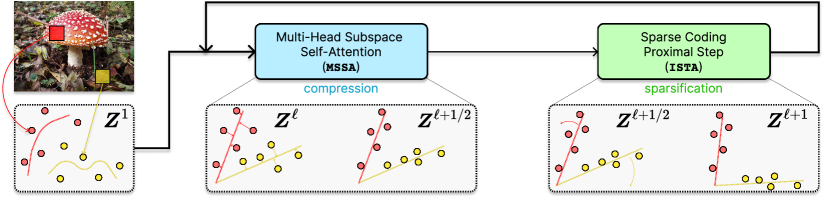
Figure 5: The ‘main loop’ of the CRATE white-box deep network design. After preprocessing input data $\bm{X}$ into a sequence of tokens $\bm{Z}^{1}$, crate constructs a deep network that transforms the data to a canonical configuration of low-dimensional subspaces by successive compression against a local model for the distribution, generating $\bm{Z}^{\ell+1/2}$, and sparsification against a global dictionary, generating $\bm{Z}^{\ell+1}$. Repeatedly stacking these blocks and training the model parameters via backpropagation yields a powerful and interpretable representation of the data.

Although easy to state, each term of the sparse rate reduction objective proposed in the previous section, viz.

$$\max_{f\in\mathcal{F}}\mathbb{E}_{\bm{Z}=f(\bm{X})}\big{[}R(\bm{Z})-{R}^{c}(\bm{Z}\mid\bm{U}_{[K]})-\lambda\lVert\bm{Z}\rVert_{1}\big{]},$$ (17)

can be computationally very challenging to optimize. Hence it is natural to take an approximation approach that realizes the global transformation $f$ through a concatenation of multiple, say $L$, simple incremental and local operations $f^{\ell}$ that push the representation distribution towards the desired parsimonious template distribution:

$$f\colon\bm{X}\xrightarrow{\hskip 2.84526ptf^{\mathrm{pre}}\hskip 2.84526pt}\bm{Z}^{1}\rightarrow\cdots\rightarrow\bm{Z}^{\ell}\xrightarrow{\hskip 2.84526ptf^{\ell}\hskip 2.84526pt}\bm{Z}^{\ell+1}\rightarrow\cdots\to\bm{Z}^{L+1}=\bm{Z},$$ (20)

where $f^{\mathrm{pre}}:\mathbb{R}^{D\times N}\rightarrow\mathbb{R}^{d\times n}$ is the pre-processing mapping that transforms the input token set $\bm{X}\in\mathbb{R}^{D\times N}$ to a first-layer representation $\bm{Z}^{1}\in\mathbb{R}^{d\times n}$, as in Figure 5.

Each incremental forward mapping $\bm{Z}^{\ell+1}=f^{\ell}(\bm{Z}^{\ell})$, or a “layer”, transforms the token distribution to optimize the above sparse rate reduction objective (17), conditioned on a model, say a mixture of subspaces whose bases are $\bm{U}_{[K]}^{\ell}$, of the distribution of its input tokens $\bm{Z}^{\ell}$:

$$\max_{f^{\ell}\in\mathcal{F}^{\ell}}\mathbb{E}_{\bm{Z}^{\ell+1}=f^{\ell}(\bm{Z}^{\ell})}\big{[}R(\bm{Z}^{\ell+1})-{R}^{c}(\bm{Z}^{\ell+1}\mid\bm{U}_{[K]}^{\ell})-\lambda\lVert\bm{Z}^{\ell+1}\rVert_{1}\big{]}.$$ (21)

Conceptually, if we follow the idea of the ReduNet (Chan et al., 2022), each $f^{\ell}$ should conduct a “gradient-ascent” like operation:

$$\bm{Z}^{\ell+1}=f^{\ell}(\bm{Z}^{\ell}) \approx\bm{Z}^{\ell}+\eta\nabla\big{[}R(\bm{Z}^{\ell})-{R}^{c}(\bm{Z}^{\ell}\mid\bm{U}_{[K]}^{\ell})-\lambda\lVert\bm{Z}^{\ell}\rVert_{1}\big{]},$$ (22)

$$\approx\bm{Z}^{\ell}+\eta\nabla\log p(\bm{Z}^{\ell}\mid\bm{U}_{[K]}^{\ell}),$$ (23)

where $p(\bm{Z}\mid\bm{U}_{[K]})$ was defined in (18). An acute reader might have noticed that the term $\nabla\log p(\bm{Z}\mid\bm{U}_{[K]})$ resembles that of a score function and the update (23) resembles that of a denoising process, i.e., it moves the current iterate $\bm{Z}^{\ell}$ towards the maximum-likelihood token set with respect to the signal model $\bm{U}_{[K]}^{\ell}$. We will thoroughly explore connections of the above gradient ascent operation to denoising and diffusion processes in Section 3. For now, we are interested in how to actually optimize the objective 17.

An alternating optimization strategy.

As already explored in the work of Chan et al. (2022), it is difficult to directly compute the gradient and optimize the rate reduction term $\Delta R$, let alone now with the non-smooth $\ell^{1}$ term $\|\bm{Z}\|_{1}$. Nevertheless, from an optimization perspective, once we decide on using an incremental approach to optimizing (17), there are a variety of alternative optimization strategies. In this work we opt for perhaps the simplest possible choice that exploit the special structure of the objective. Given a model $\bm{U}_{[K]}^{\ell}$ for $\bm{Z}^{\ell}$, we opt for a two-step alternating minimization process with a strong conceptual basis:

$$\bm{Z}^{\ell+1/2} \ \text{is chosen to incrementally minimize}\ R^{c}(\bm{Z}^{\ell+1/2}\mid\bm{U}_{[K]}^{\ell}),$$ (24)

$$\bm{Z}^{\ell+1} \ \text{is chosen to incrementally minimize}\left[\lambda\lVert\bm{Z}^{\ell+1}\rVert_{0}-R(\bm{Z}^{\ell+1})\right].$$ (25)

For the first step 24, we compress the tokens $\bm{Z}^{\ell}$ via an approximate gradient step to minimize an estimate for the coding rate $R^{c}(\bm{Z}^{\ell}\mid\bm{U}_{[K]}^{\ell})$. Namely, $R^{c}(\bm{Z}^{\ell}\mid\bm{U}_{[K]}^{\ell})$ measures the compression of $\bm{Z}^{\ell}$ against (i.e., adherence to) the statistical structure delineated in 10 with subspace bases $\bm{U}_{[K]}^{\ell}$. Thus, taking a gradient step on $R^{c}$ pushes the tokens towards having the desired statistics:

$$\bm{Z}^{\ell+1/2}\approx\bm{Z}^{\ell}-\kappa\nabla R^{c}(\bm{Z}^{\ell}\mid\bm{U}_{[K]}^{\ell}).$$ (26)

Unfortunately, the gradient of the coding rate $\nabla R^{c}$ is costly to compute, as it involves $K$ separate matrix inverses, one for each of the $K$ subspaces with basis $\bm{U}_{k}^{\ell}$. However, as we will formally derive in Section 2.3, this gradient can be naturally approximated using a so-called $\operatorname{\texttt{MSSA}}(\cdot)$ operator, which has a similar functional form to the multi-head self-attention operator (Vaswani et al., 2017) with $K$ heads (i.e., one for each subspace, coming from each matrix inverse), yet has a more explicit interpretation as approximately the (negative) gradient of a compression measure $R^{c}(\bm{Z}^{\ell}\mid\bm{U}_{[K]}^{\ell})$. As a result, we obtain a transformed token set $\bm{Z}^{\ell+1/2}$ given by

$$\bm{Z}^{\ell+1/2}\doteq\bm{Z}^{\ell}+\operatorname{\texttt{MSSA}}(\bm{Z}^{\ell}\;\mid\;\bm{U}_{[K]}^{\ell})\approx\bm{Z}^{\ell}-\kappa\nabla R^{c}(\bm{Z}^{\ell}\mid\bm{U}_{[K]}^{\ell}).$$ (27)

For the second step of (25), we sparsify the compressed tokens, choosing $\bm{Z}^{\ell+1}$ via a suitably-relaxed proximal gradient step to minimize the remaining term $\lambda\lVert\bm{Z}^{\ell+1}\rVert_{1}-R(\bm{Z}^{\ell+1})$. As we will argue in detail in Section 2.4, we can find such a $\bm{Z}^{\ell+1}$ by solving a sparse representation problem with respect to a sparsifying codebook, i.e., dictionary $\bm{D}^{\ell}$:

$$\bm{Z}^{\ell+1}\approx\mathop{\mathrm{arg\,min}}_{{\bm{Z}}}\left[\lambda\lVert\bm{Z}\rVert_{1}+\frac{1}{2}\lVert\bm{Z}^{\ell+1/2}-\bm{D}^{\ell}{\bm{Z}}\rVert_{F}^{2}\right].$$ (28)

In this work, we choose to implement this step with an iteration of the iterative shrinkage-thresholding algorithm (ISTA), which has classically been used to solve such sparse representation problems (Beck and Teboulle, 2009). We call such an iteration the $\operatorname{\texttt{ISTA}}(\cdot)$ operator, formally defined in Section 2.4. We obtain tokens $\bm{Z}^{\ell+1}$ given by

$$\bm{Z}^{\ell+1}\doteq\operatorname{\texttt{ISTA}}(\bm{Z}^{\ell+1/2}\mid\bm{D}^{\ell})\approx\mathop{\mathrm{arg\,min}}_{\bm{Z}}\left[\lambda\lVert\bm{Z}\rVert_{1}+\frac{1}{2}\lVert\bm{Z}^{\ell+1/2}-\bm{D}^{\ell}{\bm{Z}}\rVert_{F}^{2}\right].$$ (29)

Both compression and sparsification are applied incrementally and repeatedly, as these operations form layers of the network

$$f^{\ell}\colon\bm{Z}^{\ell}\xrightarrow{\hskip 2.84526pt\texttt{MSSA}\hskip 2.84526pt}\bm{Z}^{\ell+1/2}\xrightarrow{\hskip 2.84526pt\texttt{ISTA}\hskip 2.84526pt}\bm{Z}^{\ell+1}$$ (30)

as in 20. Figure 6 graphically demonstrates the idealized effect of one layer.

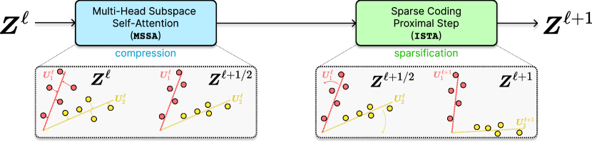
Figure 6: The effect of one encoder layer $f^{\ell}$ on the distribution of its input. First, $\bm{Z}^{\ell}$ is compressed against the codebook $\bm{U}_{[K]}^{\ell}$ to obtain $\bm{Z}^{\ell+1/2}$. Then, $\bm{Z}^{\ell+1/2}$ is sparsified using the codebook $\bm{D}^{\ell}$ to obtain $\bm{Z}^{\ell+1}$.

2.3 Self-Attention as Gradient Descent on Coding Rate of Tokens

In this subsection and the next, we provide technical details about each of the two steps mentioned in the Section 2.2, in particular the precise forms of the $\operatorname{\texttt{MSSA}}(\cdot)$ and $\operatorname{\texttt{ISTA}}(\cdot)$ operators.

For the first step, where we compress the set of tokens against the $K$ subspaces by minimizing the upper bound for the coding rate $R^{c}$:

$$\bm{Z}^{\ell+1/2}\ \text{is chosen to incrementally minimize}\ R^{c}(\bm{Z}^{\ell+1/2}\mid\bm{U}_{[K]}^{\ell}).$$ (24)

As in Section 2.2, the compression operator takes an approximate gradient descent step on $R^{c}$. The gradient of $R^{c}(\bm{Z}\mid\bm{U}_{[K]})$ is given by

$$\nabla R^{c}(\bm{Z}\mid\bm{U}_{[K]})=\beta\sum_{k=1}^{K}\bm{U}_{k}(\bm{U}_{k}^{\ast}\bm{Z})\Big{(}\bm{I}+\beta(\bm{U}_{k}^{\ast}\bm{Z})^{\ast}(\bm{U}_{k}^{\ast}\bm{Z})\Big{)}^{-1}.$$ (31)

The expression in 31 is highly expensive to compute exactly, since it requires $K$ matrix inverses, making the use of naive gradient descent intractable on large-scale problems. Therefore, we seek an efficient approximation to this gradient; we choose to use the first-order Neumann series:

$$\nabla R^{c}(\bm{Z}\mid\bm{U}_{[K]}) \approx\beta\sum_{k=1}^{K}\bm{U}_{k}(\bm{U}_{k}^{\ast}\bm{Z})\big{(}\bm{I}-\beta(\bm{U}_{k}^{\ast}\bm{Z})^{\ast}(\bm{U}_{k}^{\ast}\bm{Z})\big{)}$$ (32)

$$=\beta\left(\sum_{k=1}^{K}\bm{U}_{k}\bm{U}_{k}^{\ast}\right)\bm{Z}-\beta\sum_{k=1}^{K}\bm{U}_{k}(\bm{U}_{k}^{\ast}\bm{Z})(\bm{U}_{k}^{\ast}\bm{Z})^{\ast}(\bm{U}_{k}^{\ast}\bm{Z}).$$ (33)

The above approximate gradient expression 32 approximates the residual of each projected token feature $\bm{U}_{k}^{*}\bm{z}_{i}$ regressed by other token features $\bm{U}_{k}^{\ast}\bm{z}_{j}$ (Chan et al., 2022). But, differently from (Chan et al., 2022), not all token features in this auto-regression are from the same subspace. Hence, to compress each token feature with token features from its own group, we can compute their similarity through an auto-correlation among the projected features as $(\bm{U}_{k}^{\ast}\bm{Z})^{\ast}(\bm{U}_{k}^{\ast}\bm{Z})$ and convert it to a distribution of membership with a softmax, namely $\operatorname{softmax}\left((\bm{U}_{k}^{\ast}\bm{Z})^{\ast}(\bm{U}_{k}^{\ast}\bm{Z})\right)$. Thus, as we show in more detail in Section A.1, if we only use similar tokens to regress and denoise each other, then a gradient step on the coding rate with learning rate $\kappa$ can be naturally approximated as follows:

$$\bm{Z}^{\ell+1/2}=(1-\beta\kappa)\bm{Z}^{\ell}+\beta\kappa\operatorname{\texttt{MSSA}}(\bm{Z}^{\ell}\mid\bm{U}_{[K]}^{\ell})\approx\bm{Z}^{\ell}-\kappa\nabla R^{c}(\bm{Z}^{\ell}\mid\bm{U}_{[K]}^{\ell}),$$ (34)

where MSSA is defined through an SSA operator as:

$$\operatorname{\texttt{SSA}}(\bm{Z}\mid\bm{U}_{k}) \doteq(\bm{U}_{k}^{\ast}\bm{Z})\operatorname{softmax}\left((\bm{U}_{k}^{\ast}\bm{Z})^{\ast}(\bm{U}_{k}^{\ast}\bm{Z})\right),\quad k\in[K],$$ (35)

$$\operatorname{\texttt{MSSA}}(\bm{Z}\mid\bm{U}_{[K]}) \doteq\beta\begin{bmatrix}\bm{U}_{1},\dots,\bm{U}_{K}\end{bmatrix}\begin{bmatrix}\operatorname{\texttt{SSA}}(\bm{Z}\mid\bm{U}_{1})\\ \vdots\\ \operatorname{\texttt{SSA}}(\bm{Z}\mid\bm{U}_{K})\end{bmatrix}.$$ (36)

Here the SSA operator in (35) resembles the attention operator in a typical transformer (Vaswani et al., 2017), except that here the linear operators of value, key, and query are all set to be the same as the subspace basis, i.e., $\bm{V}_{k}=\bm{K}_{k}=\bm{Q}_{k}=\bm{U}_{k}^{*}$. We note that recently Hinton (2021) has surmised that it is more sensible to set the “value, key, and query” projection matrices in a transformer to be equal. Our derivation confirms this mathematically. Hence, we name $\operatorname{\texttt{SSA}}(\,\cdot\,\mid\bm{U}_{k}):\mathbb{R}^{d\times n}\rightarrow\mathbb{R}^{p\times n}$ the Subspace Self-Attention (SSA) operator (more details and justification can be found in 101 in Section A.1). Then, the whole MSSA operator in (36), formally defined as $\operatorname{\texttt{MSSA}}(\,\cdot\,\mid\bm{U}_{[K]})\colon\mathbb{R}^{d\times n}\to\mathbb{R}^{d\times n}$ and called the Multi-Head Subspace Self-Attention (MSSA) operator, aggregates the attention head outputs by averaging using model-dependent weights, similar in concept to the popular multi-head self-attention operator in existing transformer networks. The overall gradient step (34) resembles the multi-head self-attention implemented with a skip connection in transformers.

2.4 MLP as Proximal Gradient Descent for Sparse Coding of Tokens

In the previous subsection, we focused on how to compress a set of token features $\bm{Z}^{\ell}$ against a set of low-dimensional subspaces with orthonormal bases $\bm{U}_{[K]}^{\ell}$, obtaining a more compressed token set $\bm{Z}^{\ell+1/2}$ which approximately minimizes $R^{c}(\bm{Z}^{\ell+1/2}\mid\bm{U}_{[K]}^{\ell})$. That is, we solved 24 from Section 2.2:

$$\bm{Z}^{\ell+1/2}\ \text{is chosen to incrementally minimize}\ R^{c}(\bm{Z}^{\ell+1/2}\mid\bm{U}_{[K]}^{\ell}).$$ (24)

Now, it remains to choose $\bm{Z}^{\ell+1}$, by solving 25 from Section 2.2:

$$\bm{Z}^{\ell+1}\ \text{is chosen to incrementally minimize}\ \lambda\lVert\bm{Z}^{\ell+1}\rVert_{0}-R(\bm{Z}^{\ell+1})$$ (25)

$$=\scalebox{0.875}{$\lambda\lVert\bm{Z}^{\ell+1}\rVert_{0}-\frac{1}{2}\operatorname{logdet}\left(\bm{I}+\alpha(\bm{Z}^{\ell+1})^{\ast}(\bm{Z}^{\ell+1})\right)$}.$$ (37)

On top of optimizing the remaining terms in the overall sparse rate reduction objective 15, this step also serves an important conceptual role in itself. Namely, the term $\lVert\bm{Z}\rVert_{0}$ in the objective 25 serves to sparsify the compressed tokens, leading to a more compact and structured (i.e., parsimonious) representation. In addition, the coding rate $R(\bm{Z})$ in 25 promotes diversity and non-collapse of the representations, a highly desirable property.

Similarly to Section 2.2, the gradient $\nabla R(\bm{Z})$ involves a matrix inverse (Chan et al., 2022), and thus naive proximal gradient to solve 25 becomes intractable on large-scale problems. We therefore take a different, simplifying approach to trading off between representational diversity and sparsification: we posit a (complete) incoherent or orthogonal dictionary $\bm{D}^{\ell}\in\mathbb{R}^{d\times d}$, and ask to sparsify the intermediate iterates $\bm{Z}^{\ell+1/2}$ with respect to $\bm{D}^{\ell}$. That is, $\bm{Z}^{\ell+1/2}\approx\bm{D}^{\ell}\bm{Z}^{\ell+1}$ where $\bm{Z}^{\ell+1}$ is more sparse; that is, it is a sparse encoding of $\bm{Z}^{\ell+1/2}$. The dictionary $\bm{D}^{\ell}$ is used to sparsify all tokens simultaneously. By the incoherence assumption, we have $(\bm{D}^{\ell})^{\ast}(\bm{D}^{\ell})\approx\bm{I}$. Thus from 8 we have

$$R(\bm{Z}^{\ell+1/2})\approx R(\bm{D}^{\ell}\bm{Z}^{\ell+1})\approx R(\bm{Z}^{\ell+1}).$$ (38)

Thus we aim to solve 25 with the following program:

$$\bm{Z}^{\ell+1}\approx\mathop{\mathrm{arg\,min}}_{\bm{Z}}\lVert\bm{Z}\rVert_{0}\quad\mbox{subject to}\quad\bm{Z}^{\ell+1/2}=\bm{D}^{\ell}\bm{Z}.$$ (39)

The above sparse representation program is usually solved by relaxing it to an unconstrained convex program, known as LASSO (Wright and Ma, 2022):

$$\bm{Z}^{\ell+1}\approx\mathop{\mathrm{arg\,min}}_{\bm{Z}}\left[\lambda\lVert\bm{Z}\rVert_{1}+\frac{1}{2}\lVert\bm{Z}^{\ell+1/2}-\bm{D}^{\ell}\bm{Z}\rVert_{F}^{2}\right].$$ (40)

In our implementation, motivated by (Sun et al., 2018; Zarka et al., 2020; Guth et al., 2022), we also add a non-negative constraint to $\bm{Z}^{\ell+1}$, and solve the corresponding non-negative LASSO:

$$\bm{Z}^{\ell+1}\approx\mathop{\mathrm{arg\,min}}_{\bm{Z}\geq\mathbf{0}}\left[\lambda\lVert\bm{Z}\rVert_{1}+\frac{1}{2}\lVert\bm{Z}^{\ell+1/2}-\bm{D}^{\ell}\bm{Z}\rVert_{F}^{2}\right].$$ (41)

We incrementally optimize 41 by performing an unrolled proximal gradient descent step, known as an ISTA step (Beck and Teboulle, 2009), to give the update:

$$\bm{Z}^{\ell+1} =\operatorname{\texttt{ISTA}}(\bm{Z}^{\ell+1/2}\mid\bm{D}^{\ell}),$$ (42)

$$\text{where}\quad\operatorname{\texttt{ISTA}}(\bm{Z}\mid\bm{D}) \doteq\operatorname{ReLU}(\bm{Z}-\eta\bm{D}^{\ast}(\bm{D}\bm{Z}-\bm{Z})-\eta\lambda\bm{1}).$$ (43)

In Section A.2, we will show one can arrive at a similar operator to the above ISTA-like update for optimizing (25) by properly linearizing and approximating the coding rate $R(\bm{Z})$.

2.5 The Overall White-Box Transformer Architecture: CRATE

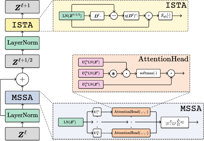
Figure 7: One layer of the CRATE encoder architecture. The full architecture is simply a concatenation of such layers, with some initial tokenizer, pre-processing head, and final task-specific head (i.e., a classification head).

By combining the above two steps:

1. (Section 2.3) Local compression of tokens within a sample towards a mixture-of-subspace structure, leading to the multi-head subspace self-attention block – MSSA;

2. (Section 2.4) Global sparsification of token sets across all samples through sparse coding, leading to the sparsification block – ISTA;

we can get the following rate-reduction-based transformer layer, illustrated in Figure 7,

$$\bm{Z}^{\ell+1/2}\doteq\bm{Z}^{\ell}+\texttt{MSSA}(\bm{Z}^{\ell}\mid\bm{U}_{[K]}^{\ell}),\qquad\bm{Z}^{\ell+1}\doteq\texttt{ISTA}(\bm{Z}^{\ell+1/2}\mid\bm{D}^{\ell}).$$ (44)

Composing multiple such layers following the incremental construction of our representation in 20, we obtain a white-box transformer architecture that transforms the data tokens towards a compact and sparse union of incoherent subspaces. An overall flow of this architecture was shown in Figure 5.

Remark 4 (Design choices in CRATE).

We note that in this work, at each stage of our network construction, we have chosen arguably the simplest possible construction to use. We can substitute each part of this construction, so long as the new part maintains the same conceptual role, and obtain another white-box architecture. Nevertheless, our such-constructed architecture, called crate, connecting to existing transformer models, is not only fully mathematically interpretable, but also obtains competitive results on real-world datasets, as we will see in Section 4.

Remark 5 (The roles of the forward pass and backward propagation).

In contrast to other unrolled optimization approaches such as the ReduNet (Chan et al., 2022), we explicitly model the distribution of each $\bm{Z}^{\ell}$ and $\bm{Z}^{\ell+1/2}$ at each layer, either by a mixture of linear subspaces or sparsely generated from a dictionary. In Section 2.2, we introduced the interpretation that at each layer $\ell$, the learned bases for the subspaces $\bm{U}_{[K]}^{\ell}$ and the learned dictionaries $\bm{D}^{\ell}$ together serve as a codebook or analysis filter that encodes and transforms the intermediate representations at each layer $\ell$. Since the input distribution to layer $\ell$ is first modeled by $\bm{U}_{[K]}^{\ell}$ then transformed by $\bm{D}^{\ell}$, the input distribution to each layer is different, and so we require a separate code book at each layer to obtain the most parsimonious encoding. Parameters of these codebooks (i.e., the subspace bases and the dictionaries), heretofore assumed as being perfectly known, are actually learned from data (say via backward propagation within end-to-end training).

Hence, our methodology features a clear conceptual separation between forward “optimization” and backward “learning” for the so-derived white-box deep neural network. Namely, in its forward pass, we interpret each layer as an operator which, conditioned on a learned model (i.e., a codebook) for the distribution of its input, transforms this distribution towards a more parsimonious representation. In its backward propagation, the codebook of this model, for the distribution of the input to each layer, is updated to better fit the input-output relationship. This conceptual interpretation implies a certain agnosticism of the model representations towards the particular task and loss; in particular, many types of tasks and losses will ensure that the models at each layer are fit, which ensures that the model produces parsimonious representations. To wit, we show in the sequel (Section 4) that the crate architecture promotes parsimonious representations and maintains layer-wise white-box operational characteristics on several different tasks, losses, and modalities.

3 White-Box Decoding via Structured Denoising and Diffusion

In Section 2, we have presented a principled metric for measuring the quality of learned representations—the sparse rate reduction 15—and showed how to derive, via incremental optimization of this objective, a white-box transformer architecture (crate) for general representation learning of high-dimensional data. Conceptually, this corresponds to a (compressive) encoder:

$$f:\bm{X}\rightarrow\bm{Z},$$

mapping high-dimensional data to representations preserving the distinct modes of intrinsic variability of the data.

For numerous reasons, ranging from being able to use the learned representations $\bm{Z}$ for generation and prediction to having flexible avenues to learn the parameters $(\bm{U}_{[K]}^{\ell})_{\ell\in[L]}$ of the white-box encoder $f$ from data, it is highly desirable to have a corresponding construction of a decoder:

$$g:\bm{Z}\rightarrow\widehat{\bm{X}},$$

mapping the representations to approximations $\widehat{\bm{X}}$ of the original data distribution. However, it is challenging to construct a white-box decoder purely following the unrolled optimization framework that we have presented and exploited in Section 2 to derive the crate encoder. Previous works, including notably the ReduNet of Chan et al. (2022), obtain white-box architectures for encoding only; on the other hand, models that have incorporated a decoder for learning (self-)consistent representations via autoencoding and closed-loop transcription (Dai et al., 2022), including in unsupervised settings, have leveraged black-box deep network architectures for both the encoder $f$ and the decoder $g$ (Dai et al., 2023), or limited-capacity architectures for the decoder $g$ (Tolooshams and Ba, 2022). Can compression alone, measured through the sparse rate reduction 15, be used to derive a white-box decoder architecture? And in such a white-box decoder architecture, what are the relevant operators for recovering the data distribution $\widehat{\bm{X}}\approx\bm{X}$ from the representation $\bm{Z}$, and can they be related to the operators in the encoder $f$?

In this section, we will resolve both of these fundamental questions affirmatively. We do this by establishing a powerful connection between compression, around which we have derived the crate encoder architecture, and diffusion-denoising, the mathematical processes by which a data distribution is transformed into pure noise by incremental corruptions, and then recovered incrementally, using information about the data distribution at each corruption level. Figure 8 illustrates this connection with an intuitive example. This connection allows us to interpret the layers of the crate encoder, which we have shown in Section 2 perform compression against learnable local signal models, say following 10, as performing denoising against the signal model. Since we are denoising against a highly structured input distribution, we call this process “structured denoising”. Given the model, this structured denoising process can be reversed in order to incrementally reconstruct the data distribution across several layers—we call this process “structured diffusion”, analogously but not identically to the denoising-diffusion process which underlies diffusion models. The structured denoising-diffusion processes naturally supply the construction of the first white-box decoder architecture for end-to-end representation learning.

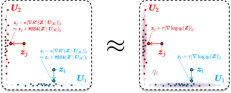
Figure 8: Compression and denoising against the low-dimensional Gaussian mixture token model 10 are equivalent. Left: the effect of compression against the low-dimensional Gaussian mixture model for tokens 10, i.e., taking gradient steps on the coding rate $R^{c}(\cdot\mid\bm{U}_{[K]})$—or equivalently, using the $\operatorname{\texttt{MSSA}}(\cdot\mid\bm{U}_{[K]})$ operator—which is shown in Theorem 6 to be equivalent to projecting onto the $\bm{U}_{[K]}$. Right: the effect of denoising against 10, i.e., taking gradient steps on the score function of the noisy model 11 at small noise levels $\sigma$, or equivalently small times $t$. Up to scaling factors (not pictured), these two operations are equivalent, and in any case have similar geometric and statistical interpretations as a projection onto the support of the data distribution. This connection motivates our structured denoising-diffusion framework, as elaborated in Section 3.2.

3.1 Denoising-Diffusion against Low-Dimensional Structures

In Section 2, we derived each layer $f^{\ell}$ of the encoder $f$ via compression of the token distribution against a local signal model (i.e., the model 10), and sparsification in the standard basis. To derive a corresponding white-box decoder $g$, we will make a connection between compression and denoising, a problem with a rich mathematical theory and powerful implications for practical representation learning. In this section, we review the fundamental concepts of this theory in order to motivate our later developments.

One-step denoising via Tweedie’s formula.

Consider, for simplicity, a single token $\bm{z}_{\natural}^{\ell}$ which has a particular marginal distribution, and define a noisy observation $\bm{z}^{\ell}\doteq\bm{z}_{\natural}^{\ell}+\sigma^{\ell}\bm{w}$, where $\sigma^{\ell}>0$ is a positive noise level, and $\bm{w}$ is a standard Gaussian vector independent of $\bm{z}_{\natural}^{\ell}$. We imagine that $\bm{z}_{\natural}^{\ell}$ represents the marginal distribution of any token at layer $\ell$ of the encoding process, and $\bm{z}^{\ell}$ has the same interpretation subject to a (small) Gaussian corruption. To denoise the observation $\bm{z}^{\ell}$ is to recover, up to statistical limits, the signal (given by 10, which we will write here as $\bm{z}_{\natural}^{\ell}$) from the noisy observation $\bm{z}^{\ell}$. In the mean-square sense, the optimal estimate is $\mathbb{E}[\bm{z}_{\natural}^{\ell}\nonscript\>|\allowbreak\nonscript\>\mathopen{}\bm{z}^{\ell}]$. Letting $\bm{z}\mapsto q^{\ell}(\bm{z})$ denote the density of $\bm{z}^{\ell}$, Tweedie’s formula (Efron, 2011a) allows us to express this in closed-form:

$$\mathbb{E}[\bm{z}_{\natural}^{\ell}\nonscript\>|\allowbreak\nonscript\>\mathopen{}\bm{z}^{\ell}]=\bm{z}^{\ell}+(\sigma^{\ell})^{2}\nabla\log q^{\ell}(\bm{z}^{\ell}).$$ (45)

Tweedie’s formula expresses the optimal representation in terms of an additive correction (in general a nonlinear function of $\bm{z}^{\ell}$) to the noisy observations by the gradient of the log-likelihood of the distribution of the noisy observations, also known as the score function $\nabla\log q^{\ell}$ (Hyvärinen, 2005). One may interpret Tweedie’s formula as denoising via a gradient ascent step on the score function at noise level $\sigma^{\ell}$. This connection is well-known in the areas of estimation theory and inverse problems (Efron, 2011a; Stein, 1981; Raphan and Simoncelli, 2011; Milanfar, 2013; Kadkhodaie and Simoncelli, 2020; Venkatakrishnan et al., 2013; Romano et al., 2017), and more recently has found powerful applications in the training of generative models for natural images (Hyvärinen, 2005; Vincent, 2011; Sohl-Dickstein et al., 2015; Song et al., 2021b, a).

The practical question, of course, is then whether it is possible to efficiently learn to denoise. The additive correction with score function in 45 depends on the current noise level and the token distribution, and for general high-dimensional distributions (such as those of natural images, as above), this token distribution is unknown and can be prohibitively costly to compute. Nevertheless, in practice, the score function is often empirically modeled and approximated with a neural network (say a transformer), or another nonparametric estimator, and estimated with a large number of samples and huge amounts of computation. Despite the empirical success of such diffusion-denoising methods in learning distributions of images (Rombach et al., 2022), there has been little theoretical justification for why transformer-like architectures would be effective to model such score functions.

Denosing against a low-dimensional Gaussian mixture.

In the work of Hyvärinen (2005), the score function is used to learn a data distribution from a restricted parametric family. As shown by Hyvärinen (2005), for certain broad classes of parametric families, the score function is efficiently computable, e.g. for a mixture of Gaussians, independent component analysis models, over-complete dictionary learning, etc. Here (i.e., in this section and hereafter), we follow the same methodology. Namely, suppose that $\bm{z}_{\natural}^{\ell}$ has the low-dimensional Gaussian mixture distribution outlined in 10, so that $\bm{z}^{\ell}$ has the distribution outlined in 11 with noise level $\sigma^{\ell}$. In this case, we can obtain a closed-form expression for the score function $\nabla\log q^{\ell}$, which, when combined with Tweedie’s formula 45 and some mild technical assumptions, gives the following approximation (shown in Section B.2):

$$\mathbb{E}[\bm{z}_{\natural}^{\ell}\nonscript\>|\allowbreak\nonscript\>\mathopen{}\bm{z}^{\ell}]\approx\begin{bmatrix}\bm{U}_{1},\dots,\bm{U}_{K}\end{bmatrix}\left[\operatorname{diag}\mathopen{}\left(\operatorname{softmax}\left(\frac{1}{2(\sigma^{\ell})^{2}}\begin{bmatrix}\lVert\bm{U}_{1}^{\ast}\bm{z}^{\ell}\rVert_{2}^{2}\\ \vdots\\ \lVert\bm{U}_{K}^{\ast}\bm{z}^{\ell}\rVert_{2}^{2}\end{bmatrix}\right)\right)\otimes\bm{I}\right]\begin{bmatrix}\bm{U}_{1}^{\ast}\bm{z}^{\ell}\\ \vdots\\ \bm{U}_{K}^{\ast}\bm{z}^{\ell}\end{bmatrix},$$ (46)

where $\otimes$ denotes the Kronecker product. In the small-noise limit $\sigma^{\ell}\to 0$, the operator implemented by 46 becomes a projection of the observation $\bm{z}^{\ell}$ onto the support of the distribution of the signal model $\bm{z}_{\natural}^{\ell}$, a significant characterization of the local behavior of denoising against the signal model 10. Moreover, perhaps surprisingly, this operation is quite similar to the MSSA block derived in Section 2.3, specialized to the case $n=1$. Indeed, the operation in 46 resembles a self-attention layer in a standard transformer architecture with $K$ heads, sequence length $n=1$, and the “query-key-value” constructs being replaced by a single linear projection $\bm{U}_{k}^{\ast}\bm{z}^{\ell}$ of the token $\bm{z}^{\ell}$.

Stochastic denoising process.

The above approach only denoises the token $\bm{z}^{\ell}$ once. Much of the practical power of denoising via the score function, however, stems from the ability to iteratively denoise in small increments. Starting with the token $\bm{z}^{\ell}$, given access to score functions of the distribution of $\bm{z}_{\natural}^{\ell}$ perturbed at at all noise levels up to $\sigma^{\ell}$, iterative denoising of $\bm{z}^{\ell}$ produces new samples from the noiseless distribution of tokens $\bm{z}_{\natural}^{\ell}$. By Tweedie’s formula 45, this means that denoising $\bm{z}^{\ell}$ is equivalent to representing the signal $\bm{z}_{\natural}^{\ell}$ in a precise distributional sense. In a simple instantiation, this representation process takes the following form (Song et al., 2021b). First, consider a diffusion process, indexed by time $t\in[0,T]$ for $T=(\sigma^{\ell})^{2}>0$, which transforms the distribution of $\bm{z}_{\natural}^{\ell}$ towards the noisy distribution of $\bm{z}^{\ell}$:

$$\begin{split}\mathop{}\!\mathrm{d}\bm{z}_{t}&=\mathop{}\!\mathrm{d}\bm{w}_{t},\quad t\in[0,T],\\ \bm{z}_{0}&\overset{d}{=}\bm{z}_{\natural}^{\ell}.\end{split}$$ (47)

Here, $(\bm{w}_{t})_{t\in[0,T]}$ is a Wiener process, and we express this process in 47 as a stochastic differential equation (SDE); for background on SDEs, see Section B.1. This SDE has a unique (strong, i.e., pathwise well-defined) solution which has distribution $\bm{z}_{t}\overset{d}{=}\bm{z}_{\natural}^{\ell}+\bm{w}_{t}$. Recalling that $(\bm{w}_{t})_{t\in[0,T]}$ is a Wiener process, $\bm{w}_{t}$ is unconditionally distributed as $\mathcal{N}(\mathbf{0},t\bm{I})$, so that $\bm{z}_{T}=\bm{z}_{(\sigma^{\ell})^{2}}\overset{d}{=}\bm{z}^{\ell}$. As above, we write $q_{t}$ to denote the density of $\bm{z}_{t}$. Then by the theory of time reversal for diffusion processes (Haussmann and Pardoux, 1986; Millet et al., 1989a), the random process $(\bm{z}_{t}^{\leftarrow})_{t\in[0,T]}$, where $\bm{z}_{t}^{\leftarrow}\doteq\bm{z}_{T-t}$, uniquely solves the following SDE:

$$\begin{split}\mathop{}\!\mathrm{d}\bm{z}_{t}^{\leftarrow}&=\nabla\log q_{T-t}(\bm{z}_{t}^{\leftarrow})\mathop{}\!\mathrm{d}t+\mathop{}\!\mathrm{d}\bm{w}^{\leftarrow}_{t},\quad t\in[0,T],\\ \bm{z}_{0}^{\leftarrow}&\overset{d}{=}\bm{z}^{\ell},\end{split}$$ (48)

where $\bm{w}^{\leftarrow}_{t}$ is another Wiener process. Because $(\bm{z}_{T-t})_{t\in[0,T]}$ solves 48, it follows that this process yields a representation (via sampling) for $\bm{z}_{\natural}^{\ell}$, as promised. Crucially, it can be rigorously shown that an iterative denoising-diffusion process such as 48 is both necessary and sufficient for representing high-dimensional multimodal data distributions efficiently (Koehler et al., 2023; Ge et al., 2018; Qin and Risteski, 2023).

Deterministic denoising process.

In 48, $\bm{z}_{t}^{\leftarrow}$ follows a noisy gradient flow to maximize (log-)likelihood of the current iterate against a smoothly time-varying, i.e., “diffused,” probabilistic model for the data distribution. We observe that each infinitesimal update of 48 is similar to Tweedie’s formula 45, which takes a single gradient step on a “diffused” log-likelihood to denoise. Thus, we interpret the process 48 as a stochastic denoising process. In practice, and in particular towards our design of a corresponding crate decoder, it will be useful to have a deterministic analogue of this process. The probability flow ODE affords such a process: following Song et al. (2021b), the dynamics of the probability density of $\bm{z}_{t}^{\leftarrow}$ in 48 is identical to that of the ODE:

$$\begin{split}\mathop{}\!\mathrm{d}\bm{z}_{t}^{\leftarrow}&=\frac{1}{2}\nabla\log q_{T-t}(\bm{z}_{t}^{\leftarrow})\mathop{}\!\mathrm{d}t,\quad t\in[0,T],\\ \bm{z}_{0}^{\leftarrow}&\overset{d}{=}\bm{z}^{\ell}.\end{split}$$ (49)

It is significant that the representation for $\bm{z}_{\natural}^{\ell}$ afforded by the deterministic process 49 can be characterized simply (again using 45) as iterative denoising, across multiple noise scales. This leads to the core insight of diffusion-denoising:

Denoising is equivalent to learning a representation of the data distribution.

With these preliminaries in hand, we will develop a deeper link between compression and denoising that we can leverage to build a consistent encoder-decoder pair $f,g$ for general ($n>1$) sets of tokens in the next section.

3.2 Parsimony and Consistency via Structured Denoising-Diffusion

In Section 3.1, we have presented the core ideas of the denoising-diffusion theory in the context of the token marignal distribution of our signal model 10. We now significantly extend the applicability of this theory, by connecting it to the compression framework we have introduced in Section 2. We will use this extension to define our structured diffusion-denoising paradigm, around which we derive a corresponding white-box decoder architecture for the encoder $f$.

To this end, we study in detail a special case of the signal model 10: we assume that the indices $s_{i}$ specifying the subspace membership of each token $\bm{z}_{i}^{\ell}$ are i.i.d. random variables, taking values in the set $\{1,\dots,K\}$ with equal probability, independently of the noises $\bm{w}_{i}$ and the coefficients $\bm{\alpha}_{i}$. We have seen in 46 in the previous subsection that for such a model with vanishing noise level $\sigma^{\ell}>0$, denoising against the token marginal distribution implements a projection onto the support of the noiseless distribution. We prove that this same property is shared by taking a gradient step on the compression objective $R^{c}(\bm{Z}^{\ell}\mid\bm{U}_{[K]}^{\ell})$, as in the construction of the MSSA block in our white-box encoder in Section 2.3, confirming the qualitative picture in Figure 8:

Theorem 6 (Informal version of Theorem 16 in Section B.3).

Suppose $\bm{Z}^{\ell}$ follows the noisy Gaussian codebook model 11, with infinitesimal noise level $\sigma^{\ell}>0$ and subspace memberships $s_{i}$ distributed as i.i.d. categorical random variables on the set of subspace indices $\{1,\dots,K\}$, independently of all other sources of randomness. Suppose in addition that the number of tokens $n$, the representation dimension $d$, the number of subspaces $K$, and the subspace dimensions $p$ have relative sizes matching those of practical transformer architectures including the crate encoder (specified in detail in 15). Then the negative compression gradient $-\nabla_{\bm{z}_{i}}R^{c}(\bm{Z}^{\ell}\mid\bm{U}_{[K]}^{\ell})$ points from $\bm{z}_{i}^{\ell}$ to the nearest $\bm{U}_{k}^{\ell}$.

Theorem 6 establishes in a representative special case of the Gaussian codebook model 10 that at low noise levels, compression against the local signal model $\bm{U}_{[K]}^{\ell}$ is equivalent to denoising against the local signal model. Viewed through the lens of the deterministic denoising process 49, this establishes a link between the gradient of the compression term $R^{c}$ and the score function for the Gaussian codebook model. Most importantly, this allows us to understand the MSSA operators of the crate encoder, derived in Section 2.3 from a different perspective, as realizing an incremental transformation of the data distribution towards the local signal model, via denoising. This important property guarantees that a corresponding deterministic diffusion process—namely, the time reversal of the denoising process 49—implies an inverse operator for the compression operation implemented by MSSA.

Using this connection to construct a principled autoencoder.

The above result suggests the following approach to constructing white-box autoencoding networks. Given the representation of the token distribution at layer $\ell$, namely $\bm{Z}^{\ell}$, we construct a deterministic structured denoising process, identical to 49, which compresses the data towards the local signal model at layer $\ell$ of the representation $f$, namely $\bm{U}_{[K]}^{\ell}$. Using the equivalence asserted in Theorem 6, we can express this structured denoising process in terms of $R^{c}$, on small timescales $T>0$ (as we work out in detail in Section B.4):

$$\odif{\bm{Z}^{\ell}(t)}=-\frac{1}{2(T-t)}\nabla R^{c}(\bm{Z}^{\ell}(t)\mid\bm{U}_{[K]}^{\ell})\odif{t}.$$ (50)

This process interpolates between the signal model 10, at $t=0$, to a noisy version of the signal model at $t=T$. By the same token, time reversal of diffusion processes gives a structured diffusion process, which transforms the signal model to an incrementally more noisy version:

$$\odif{\widetilde{\bm{Z}}^{\ell}(t)}=\frac{1}{2t}\nabla R^{c}(\widetilde{\bm{Z}}^{\ell}(t)\mid\bm{U}_{[K]}^{\ell})\odif{t}.$$ (51)

These two processes are inverses of one another in a distributional sense. To use these structured denoising and diffusion processes for representation learning, we may ambitiously treat the first-layer distribution $\bm{Z}^{1}=f^{\mathrm{pre}}(\bm{X})$ itself as being a small deviation off the distribution of the first local signal model $\bm{U}_{[K]}^{1}$. In this way, the incrementally-constructed representation 20, which we have been studying at a single “layer” $\ell$ thus far, naturally leads to the following (completely formal) structured denoising process in which layer index $\ell$ and time $t$ are unified into a single parameter, and where $\bm{Z}(0)=\bm{Z}^{1}$ is the preprocessed data distribution:

$$\odif{\bm{Z}(t)}=-\frac{1}{2(T-t)}\nabla R^{c}(\bm{Z}(t)\mid\bm{U}_{[K]}(t))\odif{t}.$$ (52)

Similarly, we have the (completely formal) inverse process, a structured diffusion process:

$$\odif{\widetilde{\bm{Z}}(t)}=\frac{1}{2t}\nabla R^{c}(\widetilde{\bm{Z}}(t)\mid\bm{U}_{[K]}(T-t))\odif{t}.$$ (53)

These two equations provide a conceptual basis for transforming data to and from a structured, parsimonious representation, via the denoising-diffusion theory. On the one hand, their similar functional forms—unified through compression, via the compression gradient $\nabla R^{c}$ and Theorem 6—demonstrate that the operators necessary for structured denoising and structured diffusion take essentially the same form. On the other hand, the connection we have made in Section 2.3 between the gradient of the compression term of the rate reduction objective and transformer-like network layers implies that a transformer-like architecture is sufficient for both compressive encoding and decoding. We can therefore realize compressive autoencoding with a fully mathematically-interpretable network architecture, which we now instantiate.

3.3 Structured Denoising-Diffusion via Invertible Transformer Layers

In Section 2, we described a method to construct a white-box transformer-like encoder network via unrolled optimization meant to compress the data against learned geometric and statistical structures, say against a distribution of tokens where each token is marginally distributed as a Gaussian mixture supported on $\bm{U}_{[K]}$. Armed with the structured diffusion-denoising correspondence outlined in Section 3.2 and its connection to compression, we now generalize the crate compressive encoder architecture to a full encoder-decoder pair, with essentially identical operators transforming the data distribution from layer to layer, and thus similarly interpretable operational characteristics.

A white-box encoder layer which implements structured denoising.

Recall that in Section 3.2, we established a continuous-time deterministic dynamical system which implements structured denoising, in that it denoises the initial data towards the desired parsimonious structure:

$$\odif{\bm{Z}(t)}=-\frac{1}{2(T-t)}\nabla R^{c}(\bm{Z}(t)\mid\bm{U}_{[K]}(t))\odif{t}.$$ (54)

In order to construct a network architecture, we use a first-order discretization (the discretization scheme being another design choice) of this process, which we describe in detail in Section B.4. This obtains the iteration

$$\bm{Z}^{\ell+1/2} \approx\bm{Z}^{\ell}-\kappa\nabla R^{c}(\bm{Z}^{\ell}\mid\bm{U}_{[K]}^{\ell}),$$ (55)

$$\text{in particular}\ \bm{Z}^{\ell+1/2} =\bm{Z}^{\ell}+\operatorname{\texttt{MSSA}}(\bm{Z}^{\ell}\mid\bm{U}_{[K]}^{\ell}),$$ (56)

where $\operatorname{\texttt{MSSA}}(\cdot)$ was defined in 36. In order to perform structured denoising while ensuring that the representation structures (e.g., supporting subspaces) themselves are parsimonious (i.e., sparse), similar to Section 2, we insert a sparsification step for the features. Namely, we instantiate a learnable dictionary $\bm{D}^{\ell}\in\mathbb{R}^{d\times d}$ and sparsify against it, obtaining

$$\bm{Z}^{\ell+1} \approx\mathop{\mathrm{arg\,min}}_{\bm{Z}\geq\mathbf{0}}\left[\lambda\lVert\bm{Z}\rVert_{1}+\frac{1}{2}\lVert\bm{Z}^{\ell+1/2}-\bm{D}^{\ell}\bm{Z}\rVert_{F}^{2}\right],$$ (57)

$$\text{in particular}\ \bm{Z}^{\ell+1} =\operatorname{\texttt{ISTA}}(\bm{Z}^{\ell+1/2}\mid\bm{D}^{\ell}),$$ (58)

where $\operatorname{\texttt{ISTA}}(\cdot)$ was defined in 42. This yields a two step iteration for the $\ell^{\mathrm{th}}$ encoder layer $f^{\ell}$, where $\bm{Z}^{\ell+1}=f^{\ell}(\bm{Z}^{\ell})$:

$$\bm{Z}^{\ell+1/2}=\bm{Z}^{\ell}+\operatorname{\texttt{MSSA}}(\bm{Z}^{\ell}\mid\bm{U}_{[K]}^{\ell}),\qquad\bm{Z}^{\ell+1}=\operatorname{\texttt{ISTA}}(\bm{Z}^{\ell+1/2}\mid\bm{D}^{\ell}).$$ (59)

This is the same layer as in the crate encoder, whose conceptual behavior we have illustrated in Figure 6. Thus, we have re-derived the crate encoder layer from a useful alternate perspective, that of structured denoising. Namely, we have shown an equivalence between structured denoising and unrolled optimization in this case, which stems from the fact that the diffusion probability flow 52 is conceptually and mechanically similar to gradient flow on the compression objective in certain regimes. Thus, we have demonstrated a useful conceptual connection between discretized diffusion processes and unrolled optimization as iteratively compressing or denoising the signal against the learned data structures.

A white-box decoder layer which implements structured diffusion.

Previously, we have shown how the structured denoising approach can recover the crate encoder architecture, derived through unrolled optimization in Section 2, as an encoder. Now, we go beyond the purview of unrolled optimization. Namely, we use the connections concretely described in Section 3.2 to construct a decoder which implements structured diffusion.

Recall that the encoder is constructed from a discretization of the structured denoising ODE given in 52. Its pathwise time reversal, which inverts the transformation of the data distribution induced by the structured denoising ODE, is given formally by the structured diffusion ODE:

$$\odif{\widetilde{\bm{Z}}(t)}=\frac{1}{2t}\nabla R^{c}(\widetilde{\bm{Z}}(t)\mid\bm{U}_{[K]}(T-t))\odif{t}.$$ (60)

For this reason, we use the structured diffusion ODE as the backbone of our decoder.

Indeed, a first-order discretization of this ODE obtains the iteration:

$$\widetilde{\bm{Z}}^{\ell+1}=\widetilde{\bm{Z}}^{\ell+1/2}-\operatorname{\texttt{MSSA}}(\widetilde{\bm{Z}}^{\ell+1/2}\mid\bm{V}_{[K]}^{\ell})\approx\widetilde{\bm{Z}}^{\ell+1/2}+\kappa\nabla R^{c}(\widetilde{\bm{Z}}^{\ell+1/2}\mid\bm{V}_{[K]}^{\ell}),$$ (61)

where $\bm{V}_{[K]}^{\ell}=(\bm{V}_{1}^{\ell},\dots,\bm{V}_{K}^{\ell})$ and each $\bm{V}_{k}^{\ell}\in\mathbb{R}^{d\times p}$ are the bases of the subspaces to “anti-compress” against. To invert the effect of a sparsifying $\operatorname{\texttt{ISTA}}(\cdot)$ step, we instantiate a learnable synthesis dictionary $\bm{E}^{\ell}\in\mathbb{R}^{d\times d}$ and multiply by it, obtaining the iteration:

$$\widetilde{\bm{Z}}^{\ell+1/2}=\bm{E}^{\ell}\widetilde{\bm{Z}}^{\ell},\qquad\widetilde{\bm{Z}}^{\ell+1}=\widetilde{\bm{Z}}^{\ell+1/2}-\operatorname{\texttt{MSSA}}(\widetilde{\bm{Z}}^{\ell+1/2}\mid\bm{V}_{[K]}^{\ell}).$$ (62)

This constructs the $(\ell+1)^{\mathrm{st}}$ layer $g^{\ell}$ of our decoder as

$$\widetilde{\bm{Z}}^{\ell+1}=g^{\ell}(\widetilde{\bm{Z}}^{\ell})\doteq\bm{E}^{\ell}\widetilde{\bm{Z}}^{\ell}-\operatorname{\texttt{MSSA}}(\bm{E}^{\ell}\widetilde{\bm{Z}}^{\ell}\mid\bm{V}_{[K]}^{\ell}).$$ (63)

A graphical depiction of the encoder and decoder layers, with layer normalization added to match the implementation, is found in Figure 9.

Remark 7 (Lack of weight-tying in autoencoding architecture).

Our derivation suggests simple pre-set values for $\bm{V}_{[K]}^{\ell}$ and $\bm{E}^{\ell}$, i.e., $\bm{U}_{[K]}^{L-\ell}$ and $(\bm{D}^{\ell})^{\ast}$ respectively. However, we do not enforce these choices, or in any way share the weights between the encoder and decoder a priori in our implementation. This is because the discretization of the structured denoising and structured diffusion dynamics in 52 and 53 is good yet imperfect; similarly, the rotation perspective on the $\operatorname{\texttt{ISTA}}(\cdot)$ (i.e., from Section 2.3) is good yet imperfect, so the such-derived inversion above is also imperfect. Thus we should not expect a $1$-$1$ correspondence between codebooks in the encoder and decoder. Correspondingly, each encoder layer and its corresponding decoder layer are only approximate mutual inverses.

Remark 8 (Alternate instantiations of structured denoising-diffusion).

In this section, to construct a decoder we established a specific connection between denoising against the model 10 and compression using a gradient step on the coding rate $R^{c}$. Mechanically, this connection was used to justify an inversion of the ISTA compression operator defined in Section 2. However, as indicated in Remark 1, one may interpret the whole sparse rate reduction 17 as a compression objective. Understanding to what degree an analogue of Theorem 6 holds for the gradient of the sparse rate reduction would be quite interesting; in particular, it would inform an analogue of this structured denoising-diffusion framework which could be used to construct potentially more powerful white-box transformer-like architectures from the sparse rate reduction. In this work, however, we use arguably the simplest possible instantiation of our structured denoising-diffusion framework, in that we make the simplest possible connection between denoising and compression.

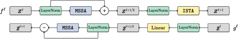
Figure 9: Diagram of each encoder layer (top) and decoder layer (bottom) in CRATE. Notice that the two layers are highly anti-parallel—each is constructed to do the operations of the other in reverse order. That is, in the decoder layer $g^{\ell}$, the $\operatorname{\texttt{ISTA}}(\cdot)$ block of $f^{L-\ell}$ is partially inverted first using a linear layer, then the $\operatorname{\texttt{MSSA}}(\cdot)$ block of $f^{L-\ell}$ is reversed; this order unravels the transformation done in $f^{L-\ell}$.

4 Experimental Evaluations

In this section, we conduct experiments to study the empirical performance of our proposed white-box transformer crate on real-world datasets and tasks. As the analysis in Section 2 and Section 3 suggests, the compression/denoising and sparsification steps can each be achieved through various alternative design choices or optimization strategies. The current crate adopts arguably the most basic choices. So our goal with the experiments is not to compete, using such a rudimentary design, with other empirically-designed transformer architectures which are heavily engineered on these tasks. Rather, the goal is to convince the reader that our transformer-like architecture crate obtains promising performance on large-scale datasets, while being fully white-box—both mathematically and empirically interpretable—and theoretically principled. We aim to achieve this goal through the following three demonstrations:

• First, we verify convincingly that the white-box transformer architecture, crate is practically effective and can achieve strong performance on many large-scale real-world datasets and tasks. These include supervised and self-supervised learning tasks on both vision and natural language data: ViT, MAE, DINO, BERT, and GPT.

• Second, unlike most empirically designed black-box networks that can usually only be evaluated through their end-to-end performance, we show that the white-box design of our network allows us to look inside the deep architecture and verify if individual layers and operators of the learned network indeed perform their design objective—say performing incremental optimization for the objective 17.

• Third, we study the white-box transformers through post hoc interpretability. Extensive qualitative and quantitative experimental results demonstrate that the internal representations of the white-box transformer are much more interpretable, with clear and easily-extractable semantic meaning, compared to black-box transformers.

In the remainder of this section we highlight a selection of results; additional experimental details and results can be found in Appendix C. PyTorch-like pseudocode is given in Appendix D.

4.1 Empirical Verification of CRATE on Many Practical Tasks

4.1.1 Supervised Image Classification via ViT

We first study the performance of crate architecture on supervised image classification, where we apply crate as the backbone architecture.

Model architecture.

We implement the architecture that is described in Section 2.5, with minor modifications that are described in Section C.1. Let $C$ be the number of classes. We use the pre-processing map:

$$f^{\mathrm{pre}}(\bm{X})=\begin{bmatrix}\bm{z}_{\texttt{[CLS]}}^{1},\bm{W}^{\mathrm{pre}}\bm{X}\end{bmatrix}+\bm{E}_{\mathrm{pos}},$$ (64)

where $\bm{z}_{\texttt{[CLS]}}^{1}\in\mathbb{R}^{d}$ is a trainable class token parameter, $\bm{X}=\begin{bmatrix}\bm{x}_{1},\dots,\bm{x}_{N}\end{bmatrix}\in\mathbb{R}^{D\times N}$ is the input image patches, $\bm{W}^{\mathrm{pre}}\in\mathbb{R}^{d\times D}$ is a trainable matrix, and $\bm{E}_{\mathrm{pos}}\in\mathbb{R}^{d\times n}$ is a trainable positional encoding matrix, where $n=N+1$. We also consider a classification head at the output of the crate model:

$$f^{\mathrm{head}}(\begin{bmatrix}\bm{z}_{1},\dots,\bm{z}_{n}\end{bmatrix})=\bm{W}^{\mathrm{head}}\bm{z}_{1},$$ (65)

where $\bm{Z}=\begin{bmatrix}\bm{z}_{1},\dots,\bm{z}_{n}\end{bmatrix}$ is the output of the encoder crate, $\bm{z}_{1}$ in particular is the feature corresponding to the class token $\bm{z}_{\texttt{[CLS]}}^{1}$, and $\bm{W}^{\mathrm{head}}\in\mathbb{R}^{C\times d}$ is a trainable classification head. The output of $f^{\mathrm{head}}$ is a set of unnormalized log-probabilities for the different classes.

We consider different model sizes of crate by varying the token dimension $d$, number of heads $K$, and the number of layers $L$. We consider four model sizes in this work: crate-Tiny, crate-Small, crate-Base, and crate-Large. We provide details about model configurations of crate in Table 8. More implementation details can be found in Section C.1; PyTorch-style pseudocode can be found in Appendix D.

Pre-training methodology.

Let $H\colon\Delta_{C}\times\Delta_{C}\to\mathbb{R}$, where $\Delta_{C}$ is the set of probability distributions on $[C]$, be the cross-entropy function, defined as

$$H(\bm{p},\bm{q})=\mathbb{E}_{x\sim\bm{p}}[-\log\bm{q}(x)]=-\sum_{c=1}^{C}p_{c}\log(q_{c}).$$ (66)

The pre-training loss is

$$L_{\mathrm{CE}}(f,f^{\mathrm{head}})\doteq\mathbb{E}_{\bm{X},\bm{y}}\mathopen{}\left[H\big{(}\bm{y},\operatorname{softmax}\big{\{}(f^{\mathrm{head}}\circ f)(\bm{X})\big{\}}\big{)}\right].$$ (67)

We pre-train on ImageNet-1K (Deng et al., 2009), using the Lion optimizer (Chen et al., 2023b). More details about the training and datasets can be found in Section C.1.

Fine-tuning methodology.

For fine-tuning (possibly on a different dataset with a different number of classes), we re-initialize $f^{\mathrm{head}}$ using parameters with the appropriate value of $C$, and train on the cross-entropy loss in 67, updating both $f$ and $f^{\mathrm{head}}$. Again, we train using the Lion optimizer (Chen et al., 2023b), this time on a variety of commonly used datasets: CIFAR10/CIFAR100 (Krizhevsky et al., 2009), Oxford Flowers (Nilsback and Zisserman, 2008), and Oxford-IIIT-Pets (Parkhi et al., 2012). More details about the training and datasets can be found in Section C.1.

Classification accuracy.

We study the empirical performance of the proposed networks by measuring their top-1 accuracy on ImageNet-1K as well as transfer learning performance on several widely used downstream datasets. We summarize the results in Table 1. Our transfer learning methodology is to fine-tune using 67 starting from the pre-trained $f$ and a re-initialized $f^{\mathrm{head}}$.

As our designed architecture leverages parameter sharing in both the attention block (MSSA) and the nonlinearity block (ISTA), our crate-Base model (22.80 million) has a similar number of parameters to the ViT-Small (22.05 million), and less than 30% of the parameters of an identically configured ViT-Base (86.54 million). From Table 1, we find that with a similar number of model parameters, our proposed network achieves similar ImageNet-1K and transfer learning performance as ViT, while having a simple and principled design. Moreover, with the same set of training hyperparameters, we observe promising scaling behavior in crate—we consistently improve the performance by scaling up the model size. For comparison, directly scaling ViT on ImageNet-1K does not always lead to consistent performance improvement measured by top-1 accuracy, even while such scaling behavior is touted as one of the main benefits of the transformer architecture (Dosovitskiy et al., 2021). Furthermore, we also study the performance of crate when pre-training on a larger dataset—ImageNet-21K (Deng et al., 2009). We then fine-tune the pre-trained crate models on downstream tasks including the ImageNet-1K dataset. The results are summarized in Table 13. In particular, the crate-B achieves 79.5% top-1 accuracy on ImageNet-1K. To summarize, we achieve promising performance on real-world large-scale datasets by directly implementing our principled architecture.

Table 1: Top-1 classification accuracy of crate on various datasets with different model scales when pre-trained on ImageNet-1K. For ImageNet-1K/ImageNet-1K ReaL, we directly evaluate the top-1 accuracy. For other datasets, we use models that are pre-trained on ImageNet as initialization and the evaluate the transfer learning performance via fine-tuning.

Model	crate-T	crate-S	crate-B	crate-L	ViT-T	ViT-S
# parameters	6.09M	13.12M	22.80M	77.64M	5.72M	22.05M
ImageNet-1K	66.7	69.2	70.8	71.3	71.5	72.4
ImageNet-1K ReaL	74.0	76.0	76.5	77.4	78.3	78.4
CIFAR10	95.5	96.0	96.8	97.2	96.6	97.2
CIFAR100	78.9	81.0	82.7	83.6	81.8	83.2
Oxford Flowers-102	84.6	87.1	88.7	88.3	85.1	88.5
Oxford-IIIT-Pets	81.4	84.9	85.3	87.4	88.5	88.6

4.1.2 Image Completion via Masked Autoencoding

Now, we study how we can use the full autoencoder architecture based on crate described in Section 3, including both the crate encoder defined in Section 2.5 and the crate decoder defined in Section 3.3, to perform masked autoencoding (He et al., 2021)—an unsupervised masked image completion task. As shorthand, we call the crate-masked autoencoder crate-MAE.

Model architecture.

We implement the encoder and decoder architectures described in Section 3, with a few changes detailed in Section C.2. We use the pre-processing map:

$$f^{\mathrm{pre}}(\bm{X})=\bm{W}^{\mathrm{pre}}\bm{X}+\bm{E}_{\mathrm{pos}},$$ (68)

where $\bm{X}=\begin{bmatrix}\bm{x}_{1},\dots,\bm{x}_{N}\end{bmatrix}\in\mathbb{R}^{D\times N}$, $\bm{W}^{\mathrm{pre}}\in\mathbb{R}^{d\times D}$ is a trainable matrix, and $\bm{E}_{\mathrm{pos}}\in\mathbb{R}^{d\times n}$ is a trainable positional encoding matrix, where $n=N$. Similarly we use the post-processing map:

$$g^{\mathrm{post}}(\widetilde{\bm{Z}})=\bm{W}^{\mathrm{post}}(\widetilde{\bm{Z}}-\bm{E}_{\mathrm{pos}}),$$ (69)

where $\bm{W}^{\mathrm{post}}\in\mathbb{R}^{D\times d}$ is another trainable matrix.

We consider different model sizes of crate by varying the token dimension $d$, number of heads $K$, and number of layers $L$; such parameters will be kept the same for the encoder and decoder. This choice is is different from the proposed MAE architecture in He et al. (2021), which uses an asymmetric encoder-decoder setup where the decoder is significantly smaller and more lightweight. This asymmetric approach is conceptually messier, whereas our symmetric approach is totally in line with our white-box derivation. We consider three model sizes: crate-MAE-Small, crate-MAE-Base, and crate-MAE-Large. Table 9 displays the model configurations and number of parameters, with a comparison to MAE, showing that crate uses around 30% of the parameters of MAE with the same model configuration (e.g., layers $L$, token dimension $d$, and number of heads $K$).

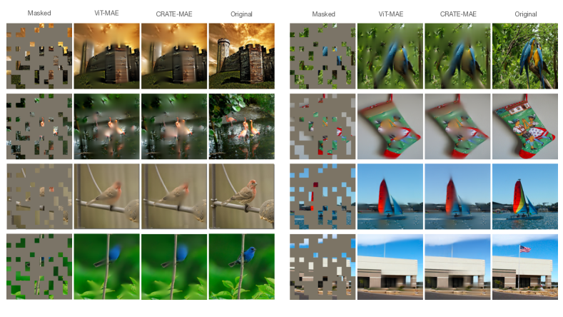
Figure 10: Autoencoding visualization comparison of crate-Base to MAE-Base (He et al., 2021) with 75% patches masked. We observe that the reconstructions from crate-Base are on par with the reconstructions from MAE-Base, despite using fewer than $1/3$ of the parameters.

Pre-training methodology.

Masked autoencoding (He et al., 2021) “masks out” a large percentage of randomly selected input image tokens in the input $\bm{X}=\begin{bmatrix}\bm{x}_{1},\dots,\bm{x}_{N}\end{bmatrix}\in\mathbb{R}^{D\times N}$ and then attempts to reconstruct the whole image, measuring success by the resulting autoencoding reconstruction loss and performance on downstream tasks. The regular masked autoencoding (MAE) loss (He et al., 2021) is defined as

$$L_{\mathrm{MAE}}(f,g)\doteq\mathbb{E}_{\bm{X},\Omega}\big{[}\lVert(g\circ f)(\operatorname{\texttt{Mask}}_{\Omega}(\bm{X}))-\bm{X}\rVert_{2}^{2}\big{]},$$ (70)

where $\texttt{Mask}_{\Omega}(\cdot)$ replaces all tokens in $\bm{X}$ whose indices are in $\Omega$ with the same masked token. Namely, for each data point, we sample a subset $\Omega\subseteq[N]$ of a fixed size, and set $\bm{X}^{\mathrm{mask}}=\begin{bmatrix}\bm{x}_{1}^{\mathrm{mask}},\dots,\bm{x}_{N}^{\mathrm{mask}}\end{bmatrix}$, where $\bm{x}_{i}^{\mathrm{mask}}=\bm{x}_{\mathrm{mask}}$ if $i\in\Omega$ and $\bm{x}_{i}^{\mathrm{mask}}=\bm{x}_{i}$ if $i\notin\Omega$, where $\bm{x}_{\mathrm{mask}}\in\mathbb{R}^{D}$ is a trainable mask token.

For pre-training, we employ the AdamW optimizer (Loshchilov and Hutter, 2019). We mainly use ImageNet-1K (Deng et al., 2009) as the main pre-training dataset. More details about training and datasets can be found in Section C.2.

Fine-tuning methodology.

Following He et al. (2021), we fine-tune using supervised classification to examine the linear separability of the features. To do this, we use either full-model fine-tuning or linear probing. The classification head is a “global pooling” head:

$$f^{\mathrm{head}}(\bm{Z})=\bm{W}^{\mathrm{head}}\left(\frac{1}{n}\sum_{i=1}^{n}\bm{z}_{i}\right)=\frac{1}{n}\bm{W}^{\mathrm{head}}\bm{Z}\,\bm{1}_{n},\qquad\text{where}\ \bm{Z}=\begin{bmatrix}\bm{z}_{1},\dots,\bm{z}_{n}\end{bmatrix},$$ (71)

where $\bm{1}_{n}$ is the all-ones vector in $\mathbb{R}^{n}$; note that this is different to the classification setup in Section 4.1.1, owing to not incorporating a class token. We train using the cross-entropy loss, where $H$ is defined in 66:

$$L_{\mathrm{CE}}(f,f^{\mathrm{head}})\doteq\mathbb{E}_{\bm{X},\bm{y}}\mathopen{}\left[H(\bm{y},\operatorname{softmax}\{(f^{\mathrm{head}}\circ f)(\bm{X})\})\right].$$ (72)

For full fine-tuning, we update both $f$ and $f^{\mathrm{head}}$. For linear probing, we update only $f^{\mathrm{head}}$. We fine-tune crate-MAE on several commonly used downstream datasets: CIFAR10/CIFAR100 (Krizhevsky et al., 2009), Oxford Flowers (Nilsback and Zisserman, 2008), and Oxford-IIIT-Pets (Parkhi et al., 2012). For fine-tuning $f^{\mathrm{head}}$, we use the AdamW optimizer on minibatches (Loshchilov and Hutter, 2019). For linear probing, we use a logistic regresion solver to compute $f^{\mathrm{head}}$ in one shot using the full dataset. More details about training can be found in Section C.2.

Autoencoding performance.

We analyze the autoencoding reconstruction performance of crate-MAE and compare with the original MAE in He et al. (2021). In Figure 10, we qualitatively compare the masked autoencoding performance of crate-MAE-Base to MAE-Base (He et al., 2021). We observe that both models are able to reconstruct the data well, despite crate using less than a third of the parameters of MAE. In Table 2, we display the average reconstruction loss of crate-MAE-Base and MAE-Base, showing a similar quantitative conclusion.

Table 2: Average reconstruction loss over the training and validation sets of ImageNet-1K as a function of architecture model size. We see that the performance of crate-Base, while a bit worse than MAE-Base, obtains promising performance on the challenging masked autoencoding task.

Reconstruction Loss	crate-Base	MAE-Base
Training	0.266	0.240
Validation	0.303	0.267

Fine-tuning performance.

In Table 3, we compare the fine-tuning and linear probing performance of crate-MAE models pretrained on ImageNet-1K across different model sizes and datasets. We demonstrate that crate-MAE has comparable finetuning performance to the usual MAE models while also saving many parameters. This demonstrates that our representations are highly geometrically and statistically structured (e.g., having linear structure), and carry semantic content that is useful for downstream tasks.

Table 3: Top-1 classification accuracy of crate-MAE-Small, crate-MAE-Base, crate-MAE-Large, and (ViT-)MAE-Base when pre-trained on ImageNet-1K and fine-tuned on classification (either on the whole network, or using logistic regression a.k.a. full-batch linear probing) for several smaller datasets. Our results show that the representation learning in crate is useful for downstream tasks on a level comparable to that of the regular MAE, on top of having several side benefits such as parameter efficiency and emergent properties (as discussed in the sequel).

Model	crate-MAE-S	crate-MAE-B	crate-MAE-L	MAE-B
# parameters	25.4M	44.6M	78.5M	143.8M
Fine-Tuning
CIFAR10	96.2	96.8	97.2	98.6
CIFAR100	79.0	80.3	81.6	87.0
Oxford Flowers-102	71.7	78.5	80.4	92.5
Oxford-IIIT-Pets	73.7	76.7	79.9	90.3
Linear Probing
CIFAR10	65.3	71.1	70.1	65.7
CIFAR100	42.3	48.6	47.7	41.0
Oxford Flowers-102	55.2	59.2	62.3	58.7
Oxford-IIIT-Pets	36.8	38.4	45.4	41.1

4.1.3 Self-Supervised Learning via DINO Training Method

Self-supervised learning (SSL) has gained increasing popularity and become a dominant approach for pre-training deep networks. In this part, we study whether the success of SSL in transformers can be applied to the proposed crate architecture. Specifically, we train crate backbones with DINO (Caron et al., 2021), a widely used SSL framework for ViTs that demonstrate great feature learning capabilities.

Model architecture.

To start with, we briefly introduce the self-supervised learning method DINO (self-distillation with no labels) (Caron et al., 2021). DINO applies knowledge distillation (Hinton et al., 2015), with a “teacher” encoder network $f_{t}^{\mathrm{proj}}\circ f_{t}$ and “student” encoder network $f_{s}^{\mathrm{proj}}\circ f_{s}$, to learn from two different “views” of an image. Here, for each “backbone” model $f$ (either $f_{s}$ or $f_{t}$), we can write (as in other experimental settings) $f=f^{L}\circ\cdots\circ f^{1}\circ f^{\mathrm{pre}}$, where the pre-processing map $f^{\mathrm{pre}}:\mathbb{R}^{D\times N}\to\mathbb{R}^{d\times n}$ is defined as

$$f^{\mathrm{pre}}(\bm{X})=\begin{bmatrix}\bm{z}_{\texttt{[CLS]}}^{1},\bm{W}^{\mathrm{pre}}\bm{X}\end{bmatrix}+\bm{E}_{\mathrm{pos}},$$ (73)

where $n=N+1$ and $\bm{z}_{\texttt{[CLS]}}^{1}\in\mathbb{R}^{d}$, $\bm{W}^{\mathrm{pre}}\in\mathbb{R}^{d\times D}$ and $\bm{E}_{\mathrm{pos}}\in\mathbb{R}^{d\times n}$ are trainable parameters, and each layer $f^{\ell}\colon\mathbb{R}^{d\times n}\to\mathbb{R}^{d\times n}$ is a transformer layer, such as the crate layer or ViT layer. Each projection map $f^{\mathrm{proj}}\colon\mathbb{R}^{d\times n}\to\mathbb{R}^{d}$ (either $f_{s}^{\mathrm{proj}}$ or $f_{t}^{\mathrm{proj}}$) is defined, as in Caron et al. (2021), as

$$f^{\mathrm{proj}}(\begin{bmatrix}\bm{z}_{1},\dots,\bm{z}_{n}\end{bmatrix})=\bm{W}_{3}^{\mathrm{proj}}\operatorname{ReLU}(\bm{W}_{2}^{\mathrm{proj}}\operatorname{ReLU}(\bm{W}_{1}^{\mathrm{proj}}\bm{z}_{1}+\bm{b}_{1}^{\mathrm{proj}})+\bm{b}_{2}^{\mathrm{proj}})+\bm{b}_{3}^{\mathrm{proj}},$$ (74)

where $\bm{W}_{i}^{\mathrm{proj}}\in\mathbb{R}^{d\times d}$ are trainable weights and $\bm{b}_{i}^{\mathrm{proj}}\in\mathbb{R}^{d}$ are trainable biases.

In our experiments, for the “backbone” layers $f^{\ell}\circ\cdots\circ f^{1}$ for the teacher and student models, we adopt the same model configuration as in the supervised learning experiments introduced in Section 4.1.1. Specially, due to the heavy computational demand for DINO, we train with two smaller model sizes for this task: crate-Small and crate-Base (note crate-Base has a similar number of parameters as as ViT-Small). Refer to Caron et al. (2021) for more implementation details about DINO, including additional small task-specific alterations.

Pre-training methodology.

We parameterize $(f_{s},f_{s}^{\mathrm{proj}})$ by a parameter set $\bm{\theta}_{s}$, and similarly parameterize $(f_{t},f_{t}^{\mathrm{proj}})$ by a parameter set $\bm{\theta}_{t}$. Note that by construction, $\bm{\theta}_{s}$ and $\bm{\theta}_{t}$ parameterize the same architecture and thus are elements of the same Euclidean space. The training objective is to minimize

$$L(\bm{\theta}_{s},\bm{\theta}_{t})\doteq\mathbb{E}_{\bm{X}}\big{[}H(P(\underbrace{\texttt{Aug}_{\texttt{g}}(\bm{X})}_{\text{view 1}};\bm{\theta}_{t},\tau_{t}),P(\underbrace{\texttt{Aug}_{\texttt{l}}(\bm{X})}_{\text{view 2}};\bm{\theta}_{s},\tau_{s}))\big{]},$$ (75)

where $\texttt{Aug}_{\texttt{g}}(\cdot)$ denotes a global view augmentation and $\texttt{Aug}_{\texttt{l}}(\cdot)$ denotes a local view augmentation , and the probability $P(\cdot;\cdot,\cdot)$ is defined as

$$P(\bm{X};\bm{\theta},\tau)=\operatorname{softmax}\left(\tau^{-1}(f_{\bm{\theta}}^{\mathrm{head}}\circ f_{\bm{\theta}})(\bm{X})\right),$$ (76)

where $f_{\bm{\theta}_{s}}=f_{s}$, and so on, and $\tau>0$ is the softmax temperature which controls how sharply the softmax concentrates about its largest values. By passing two different views (local and global) of the same image to the student network and teacher network respectively, the DINO objective is designed to encourage “local-to-global” correspondences—the features of the local view $\texttt{Aug}_{\texttt{l}}(\bm{X})$ for the student network are encouraged to be similar to the features of the global view $\texttt{Aug}_{\texttt{g}}(\bm{X})$ for the teacher network.

The training is done in the following (slightly unintuitive) way using exponential moving averages:

$$\bm{\theta}_{s}^{k+1} =\bm{\theta}_{s}^{k}-\eta\nabla_{\bm{\theta}_{s}}L(\bm{\theta}_{s}^{k},\bm{\theta}_{t}^{k}),$$ (77)

$$\bm{\theta}_{t}^{k+1} =\lambda\bm{\theta}_{t}^{k}+(1-\lambda)\bm{\theta}_{s}^{k+1},$$ (78)

where $\eta>0$ is a learning rate, $\lambda\in(0,1)$ is an exponential moving average parameter, and $k$ is the training iteration. Caron et al. (2021) applies the stop-gradient operator on the teacher network, so gradients are propagated only through the student network and not the teacher. In reality, $L$ is replaced with an empirical version over mini-batches, and the iteration for $\bm{\theta}_{s}$ can use a more complex algorithm than stochastic gradient descent. In particular, we adopt a similar training recipe as reported in Caron et al. (2021); we train on ImageNet-1K (Deng et al., 2009) and use the AdamW optimizer (Loshchilov and Hutter, 2019), with a learning rate schedule that is composed of a linear warm-up phase followed by a cosine decay schedule. Due to the differences in the backbone architecture, we only alter the choice of base learning rates and weight decay parameters in our experiments. More details can be found in Section C.3.

Fine-tuning methodology.

Similar to the evaluation protocol of Caron et al. (2021), we evaluate the classification performance using the features of the pre-trained networks. Precisely, we consider the extracted class token feature $\bm{z}_{t}$ from the pre-trained teacher network $f_{t}$ in the following way. Specifically, we obtain

$$\bm{z}_{t}\leftarrow\bm{z}_{1}\qquad\text{where}\ \begin{bmatrix}\bm{z}_{1},\dots,\bm{z}_{n}\end{bmatrix}=f_{t}(\bm{X}).$$ (79)

From here, we fine-tune on supervised classification in two different ways.

First, we use the feature vectors $\bm{z}_{t}$ to form a weighted $k$-nearest neighbor classifier (Wu et al., 2018). That is, with $C$ classes we build a classification head $f_{k}^{\mathrm{head}}\colon\mathbb{R}^{d}\to[C]$ which performs weighted $k$-nearest neighbors with respect to the training dataset. We do this for several choices of $k$, and in our shown results we select the classifier $f_{k}^{\mathrm{head}}\circ f_{t}$ with the highest accuracy on the training set.

Second, we use the feature vectors $\bm{z}_{t}$ to build a linear probing model. That is, with $C$ classes we build a classification head $f^{\mathrm{head}}\colon\mathbb{R}^{d}\to\mathbb{R}^{C}$ defined as

$$f^{\mathrm{head}}(\bm{z})=\bm{W}^{\mathrm{head}}\bm{z},$$ (80)

for a trainable parameter $\bm{W}^{\mathrm{head}}\in\mathbb{R}^{C\times d}$, by minimizing the cross-entropy loss 67

$$L_{\mathrm{CE}}(f,f^{\mathrm{head}})\doteq\mathbb{E}_{\bm{X},\bm{y}}\mathopen{}\left[H(\bm{y},\operatorname{softmax}\{(f^{\mathrm{head}}\circ f)(\bm{X})\})\right],$$ (81)

over $f^{\mathrm{head}}$ (leaving $f$ fixed). We do this by using a logistic regression solver to compute $f^{\mathrm{head}}$ in one shot using the full fine-tuning dataset.

The fine-tuning dataset in our experiments is the same as the training dataset, i.e., ImageNet-1K (Deng et al., 2009).

Fine-tuning results.

We report the Top-1 test accuracy of both our fine-tuning methodologies on ImageNet-1K in Table 4. These results show that, with only minimal changes of hyper-parameter settings, the proposed crate architecture can learn meaningful and informative features via self-supervised learning.

Later in Section 4.3, we will show how the features learned by the self-supervised DINO can already produce good image segmentation results, see Figure 18.

Table 4: Top-1 classification accuracy on ImageNet-1K of crate-Small, crate-Base, and ViT-Small when pre-trained using the DINO objective.

Model	#parameters	$k$-NN	Linear Probing
crate-Small/16	13.12M	53.02%	58.41%
crate-Base/8	22.80M	59.91%	67.42%
ViT-Small/16	22.05M	69.36%	72.02%
ViT-Small/8	22.05M	71.98%	75.63%

4.1.4 Pre-Training Language Models via BERT and GPT

We now study the performance of crate architectures on text data. Specifically, we consider two widely used pre-training tasks for learning language representations—Bidirectional Encoder Representations from Transformers (BERT) pre-training (Devlin et al., 2019; Liu et al., 2019) and Generative Pre-Training (GPT) pre-training (Radford et al., 2019).

CRATE-BERT model architecture.

For BERT pre-training, we apply the RoBERTa tokenizer (Sennrich et al., 2016; Liu et al., 2019) with vocabulary size $V=50,265$ as the default tokenizer. We implement the crate architecture that is used in image classification Section 4.1.1, except for the pre-processing layer and the task-specific head. Specifically, the pre-processing layer is described as:

$$f^{\mathrm{pre}}(\bm{X})=f^{\mathrm{embed}}(\bm{X})+\bm{E}_{\mathrm{pos}},$$ (82)

where $f^{\mathrm{embed}}$ is an embedding function which maps input tokens $\bm{x}_{i}$ to embedding vectors in $\mathbb{R}^{d}$, and $\bm{E}_{\mathrm{pos}}\in\mathbb{R}^{d\times n}$ is the sinusoid positional embedding defined in Vaswani et al. (2017). The final output layer takes the form of a linear head:

$$f^{\mathrm{head}}(\bm{Z})=\bm{W}^{\mathrm{head}}\bm{Z},$$ (83)

where $\bm{W}^{\mathrm{head}}\in\mathbb{R}^{V\times d}$.

We denote the crate model with BERT pre-training as crate-BERT. We summarize the configurations of crate-BERT models in Table 10 (upper). For crate-BERT-Base, we use the same width, number of attention heads, and depth as BERT-Base (Liu et al., 2019). crate-BERT-Base uses 60.9M parameters, while BERT-Base uses 110M parameters, nearly twice as many.

CRATE-BERT pre-training methodology.

The training loss for crate-BERT is masked language modeling (masked LM), which is defined as

$$L_{\text{BERT}}(f,f^{\mathrm{head}})=\mathbb{E}_{\bm{X},\Omega}\left[\frac{1}{\lvert\Omega\rvert}\sum_{i\in\Omega}H(\bm{1}(\bm{x}_{i}),\operatorname{softmax}\{(f^{\mathrm{head}}\circ f)(\bm{X})_{i}\})\right],$$ (84)

where $(f^{\mathrm{head}}\circ f)(\bm{X})_{i}\in\mathbb{R}^{V}$ denotes the $i^{\mathrm{th}}$ index of the model output—that is, the log-probabilities of each potential token in the vocabulary to take up the $i^{\mathrm{th}}$ index in the sequence $\bm{X}$. Similarly $\mathbf{1}(\bm{x}_{i})\in\{0,1\}^{V}$ represents the one-hot embedding vector of the token $\bm{x}_{i}$ in the vocabulary.

To pre-train, we use the Adam optimizer (Kingma and Ba, 2015). We use the same pre-training dataset as BERT  (Devlin et al., 2019), including BooksCorpus (Zhu et al., 2015) and English Wikipedia. Refer to Devlin et al. (2019) for more details about the pre-training tasks.

CRATE-GPT model architecture.

For crate-GPT pretraining, following the setup in the GPT-2 paper (Radford et al., 2019), we modify our crate architecture to align with the next word prediction task used in GPT. Specifically, we replace the attention in MSSA with a causally masked self-attention, i.e., replacing

$$\operatorname{softmax}\left((\bm{U}_{k}^{\ast}\bm{Z})^{\ast}(\bm{U}_{k}^{\ast}\bm{Z})\right) \to\operatorname{softmax}\left(\texttt{CausalMask}((\bm{U}_{k}^{\ast}\bm{Z})^{\ast}(\bm{U}_{k}^{\ast}\bm{Z}))\right),$$ (85)

$$\text{where}\ \texttt{CausalMask}(\bm{A})_{ij} =\begin{cases}A_{ij},&i\leq j\\ -\infty,&i>j.\end{cases}$$ (86)

in 35. We use the same pre-processing and head architecture as crate-BERT:

$$f^{\mathrm{pre}}(\bm{X})=f^{\mathrm{embed}}(\bm{X})+\bm{E}_{\mathrm{pos}},\qquad f^{\mathrm{head}}(\bm{Z})=\bm{W}^{\mathrm{head}}\bm{Z}.$$ (87)

We denote the crate model for GPT pre-training as crate-GPT. We summarize the configurations of GPT models in Table 10 (lower), and set the model architecture parameters such that crate-GPT has the same layer specifications as GPT2 with parameter size 60M (c.f. GPT2’s 124M, more than twice as many).

CRATE-GPT pre-training methodology.

The training objective of GPT is next word prediction (causal language modeling, causal LM), which is defined as

$$L_{\text{GPT}}(f,f^{\text{head}})=\mathbb{E}_{\bm{X}}\bigg{[}\frac{1}{\lvert\bm{X}\rvert-1}\sum_{i=1}^{\lvert\bm{X}\rvert-1}H(\bm{1}(\bm{x}_{i+1}),\operatorname{softmax}\{(f^{\mathrm{head}}\circ f)(\bm{X})_{i}\})\bigg{]},$$ (88)

where $\lvert\bm{X}\rvert$ denotes the total number of tokens in the input sample $\bm{X}$. For GPT pretraining, we mainly follow the implementations in Karpathy (2022); in particular we set the block size as 1,024. We pre-train crate-GPT models on OpenWebText (Gokaslan and Cohen, 2019) using the Adam optimizer (Kingma and Ba, 2015). Refer to Radford et al. (2019) for more details about the pre-training tasks.

As usual, we defer the pre-training setup details of crate-BERT and crate-GPT to Section C.4.

CRATE-BERT evaluation results.

Pre-training results of crate-BERT is summarized in Table 5. We use the officially released BERT checkpoints for BERT evaluation (Google, 2021). We evaluate the crate-BERT model by fine-tuning on downstream tasks from the GLUE benchmark (Wang et al., 2019). Single-task Finetuning of Table 5 means that we fine-tune the model only on the task we evaluate. In addition, following previous work (Liu et al., 2019), models pre-trained only on the masked language modeling task should be further fine-tuned on MNLI before evaluating on MRPC, STS-B and RTE to be competitive to BERT. That is, first fine-tuning on MNLI improves the performance on these tasks. Therefore, we also investigate this training recipe and include the corresponding results in the Further Finetuning after MNLI section of Table 5. The AVG score is the average of all GLUE tasks shown in the table. We also present the pre-training loss and GLUE evaluation scores of crate-BERT with respect to progressing pre-training steps in Figure 11 (left and middle). The progressing GLUE average scores are calculated under the single-task finetuning setting. From Table 5, we find that crate-BERT-Base can achieve competitive performance compared to BERT models realized by standard transformers.

Table 5: Performance on the GLUE benchmark (higher is better). All scores are obtained using the HuggingFace evaluation script (Huggingface, 2020). F1 scores are reported for QQP and MRPC, Spearman correlations are reported for STS-B, and accuracy scores are reported for the other tasks.

	SST-2	MRPC	STS-B	QQP	MNLI	QNLI	RTE	WNLI	Avg
	Acc	F1	Sprm	F1	M/MM	Acc	Acc	Acc	All
Single-task Finetuning
BERT-Medium (41M)	90.5	87.8	87.6	86.2	80.8/81.2	88.6	64.6	30.1	77.5
BERT-Base (110M)	92.3	90.9	88.5	88.2	84.4/84.6	91.7	64.3	53.5	82.0
crate-BERT-Base (61M)	85.9	80.0	73.0	85.8	76.1/75.3	83.4	53.8	56.3	74.4
Further Finetuning after MNLI
BERT-Medium (41M)	90.5	89.6	88.0	86.2	80.8/81.2	88.6	72.6	30.1	78.6
BERT-Base (110M)	92.3	90.3	86.8	88.2	84.4/84.6	91.7	79.4	53.5	83.5
crate-BERT-Base (61M)	85.9	84.7	83.2	85.8	76.1/75.3	83.4	65.0	56.3	77.3

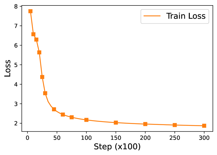
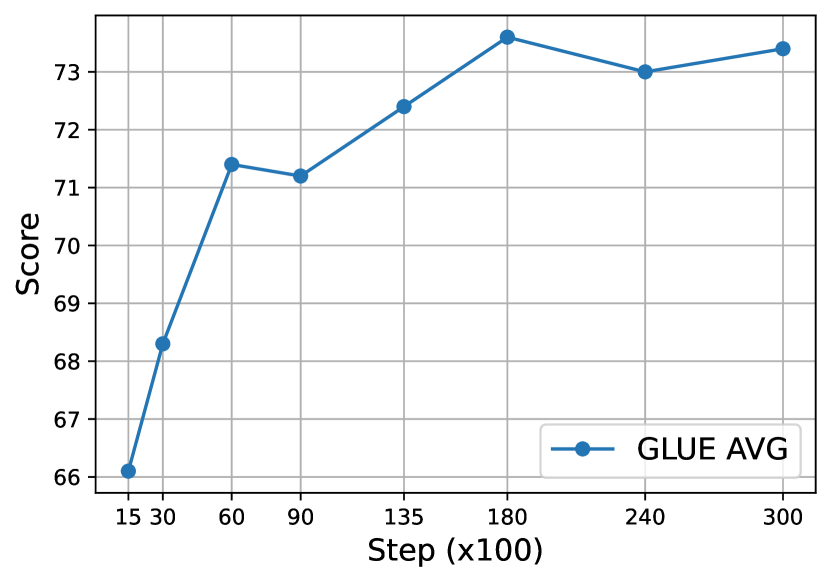
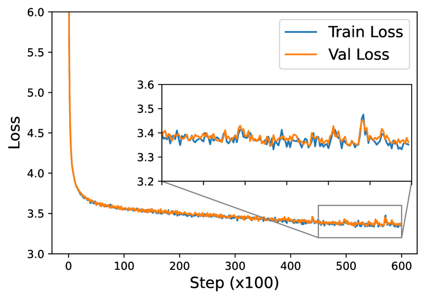
Figure 11: (left) The training loss curve of crate-BERT-Base trained on the Wikipedia and BookCorpus datasets. (middle) GLUE single-task finetuning scores evaluated after each pretraining checkpoint of crate-BERT-Base. (right) The loss curve of crate-GPT-Base trained on the OpenWebText dataset.

CRATE-GPT evaluation results.

We evaluate crate-GPT models by measuring the zero-shot cross-entropy loss on different datasets. We evaluate crate-GPT-Base on OpenWebText (OWT) as well as other datasets as shown in (Radford et al., 2019). We compare with the official release of GPT2-Base which is pre-trained on WebText (OpenAI, 2019), while crate-GPT-Base is pre-trained on OWT. Therefore, we first fine-tune GTP2-Base on OWT before evaluating on the OWT test dataset. The evaluation results on the test datasets are shown in Table 6. We also present the pre-training loss of crate-GPT with respect to progressing pre-training steps in Figure 11 (right). From both Table 6 and Figure 11 (right), we can observe that the crate architecture can be applied as backbones for generative language models and achieve competitive performance compared to GPT2.

For more technical details about the evaluation of the pre-trained crate-BERT and crate-GPT, please refer to Section C.4.

Table 6: Zero-shot cross-entropy loss of the crate-GPT2-Base model and GPT2-Base model evaluated on the test split of the datasets (lower is better).

	OWT	LAMBADA	WikiText	PTB	Avg
GPT2-Base	2.85	4.12	3.89	4.63	3.87
crate-GPT2-Base	3.37	4.91	4.61	5.53	4.61

Generated texts by CRATE-BERT and CRATE-GPT.

We also explored some qualitative examples generated by crate-BERT and crate-GPT, as shown in Figure 12. We observe a similar behavior of crate and the standard Transformers, where both answers make sense and the standard transformer slightly outperforms crate.

Figure 12: Examples of predictions made by our models and the official models. The token in Italic is the ground truth token. We compare crate-GPT2-Base to GPT2-Base on the next word prediction task and crate-BERT-Base to BERT-Medium on the masked language modeling task.

4.2 Analysis and Visualization of Learned CRATE Layers

We now study the internal representations of crate at different layers—$\{\bm{Z}^{\ell}\}_{\ell=1}^{L}$. We measure the designed representation learning objective, sparse rate reduction 16, of token representations from different layers. We mainly consider the crate encoder architectures on image classification tasks (Section 4.1.1) for the experiments in this subsection.

Do layers of CRATE achieve their design goals?

As described in Section 2.3 and Section 2.4, the MSSA block is designed to optimize the compression term $R^{c}(\bm{Z}\mid\bm{U}_{[K]})$ and the ISTA block to sparsify the token representations (corresponding to the sparsification term $\|\bm{Z}\|_{0}$). To understand whether crate indeed optimizes these terms, for each layer $\ell$, we measure (i) the compression term $R^{c}(\bm{Z}^{\ell+1/2}\mid\bm{U}_{[K]}^{\ell})$ on the MSSA block outputs $\bm{Z}^{\ell+1/2}$; and (ii) sparsity $\|\bm{Z}^{\ell+1}\|_{0}$ on the ISTA block outputs $\bm{Z}^{\ell+1}$. Specifically, we evaluate these two terms by using training/validation samples from ImageNet-1K. Both terms are evaluated at the per-sample level and averaged over $B=1000$ samples.

In Figure 13 we show the plots of these two key measures at all layers for the learned crate-small model. We find that as the layer index $\ell$ increases, both the compression and the sparsification terms improve in most cases. The increase in the sparsity measure of the last layer is caused by the extra linear layer for classification. These results suggest that crate aligns well with the original design goals: once learned, it essentially learns to gradually compress and sparsity the representations through its layers. In addition, we also measure the compression and sparsification terms on crate models with different model sizes as well as intermediate model checkpoints and the results are shown by plots in Figure 20 of Section C.6. The observations are very consistent across all different model sizes—both the compression and sparsification terms improve in most scenarios. Models with more layers tend to optimize the objectives more effectively, confirming our understanding of each layer’s roles.

To see the effect of learning, we present the evaluations on crate-Small trained with different numbers of epochs in Figure 14. When the model is not trained enough (e.g. untrained), the architecture does not optimize the objectives effectively. However, during training—learning better subspaces $\bm{U}_{[K]}^{\ell}$ and dictionaries $\bm{D}^{\ell}$—the designed blocks start to optimize the objectives much more effectively.

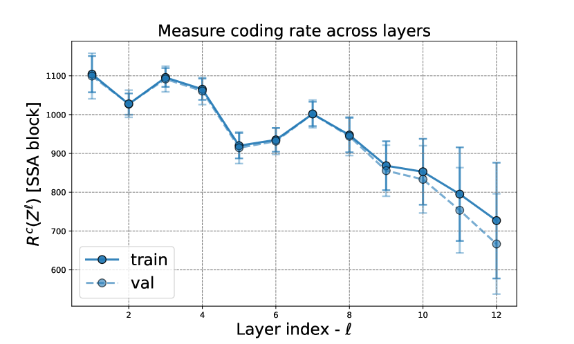
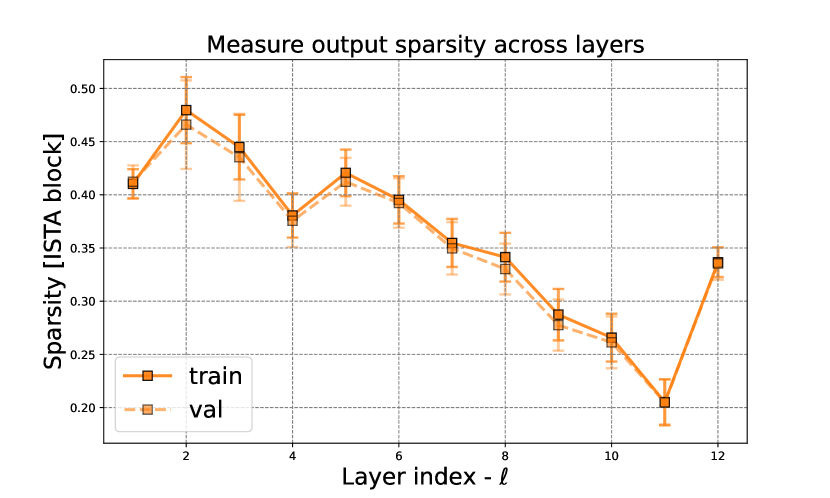
Figure 13: Left: The compression term $R^{c}(\bm{Z}^{\ell+1/2}\mid\bm{U}_{[K]}^{\ell})$ of the MSSA outputs at different layers. Right: the sparsity of the ISTA output block, $\|\bm{Z}^{\ell+1}\|_{0}/(d\cdot N)$, at different layers. (Model: crate-Small).

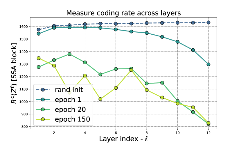
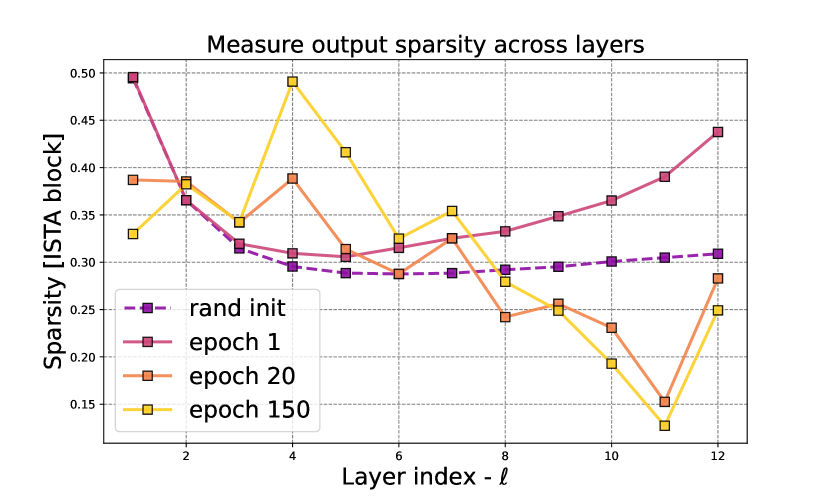
Figure 14: The compression term $R^{c}(\bm{Z}^{\ell+1/2}\mid\bm{U}_{[K]}^{\ell})$ (left) and sparsification term $\|\bm{Z}^{\ell+1}\|_{0}/(d\cdot N)$ (right) across models trained with different numbers of epochs. (Model: crate-Base).

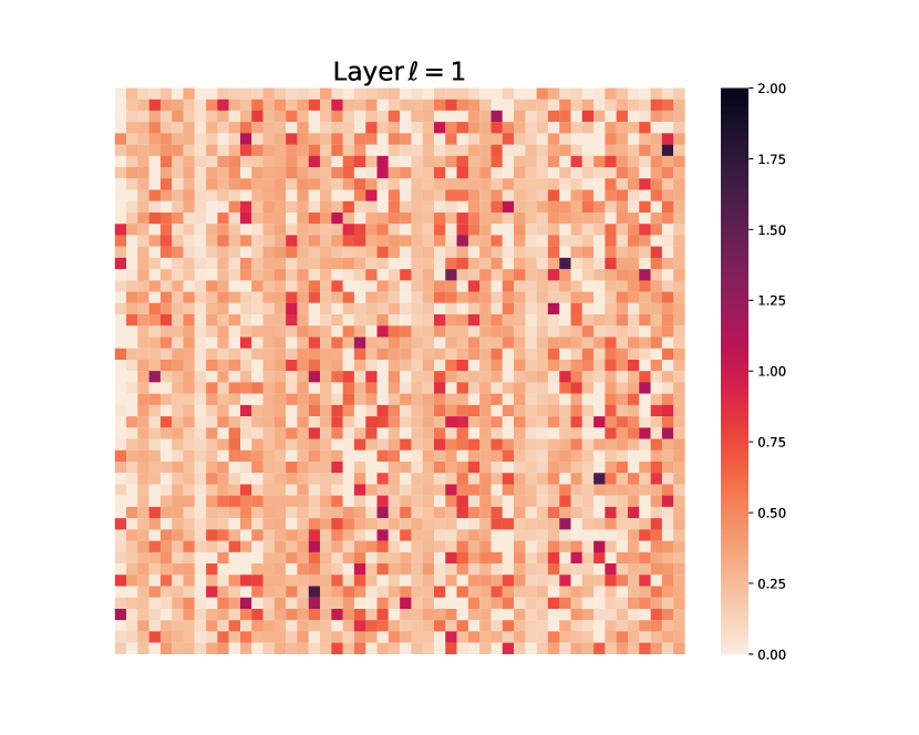
(a) $\ell=1$.

(b) $\ell=2$.

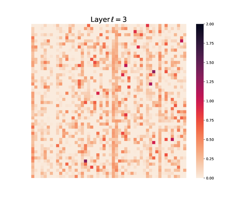
(c) $\ell=3$.

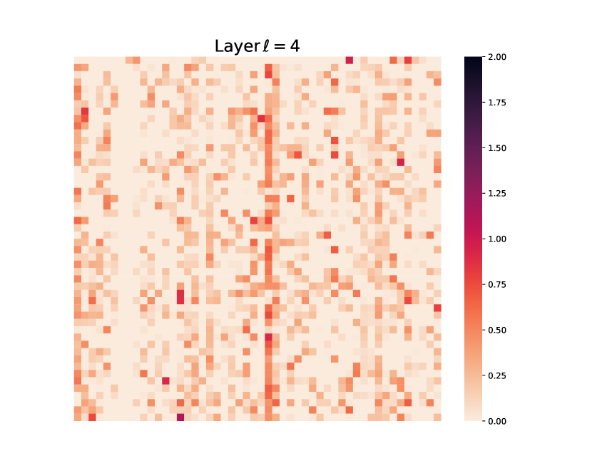
(d) $\ell=4$.

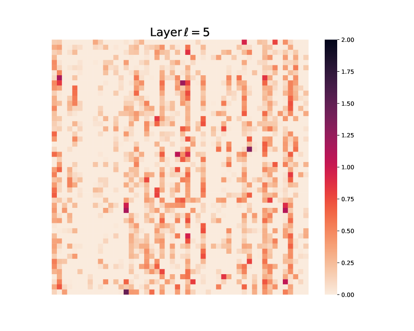
(e) $\ell=5$.

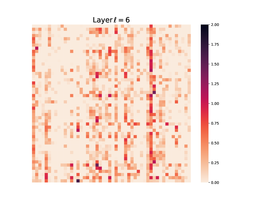
(f) $\ell=6$.

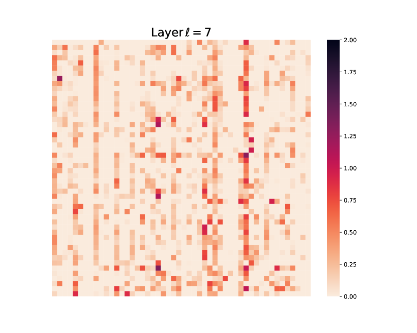
(g) $\ell=7$.

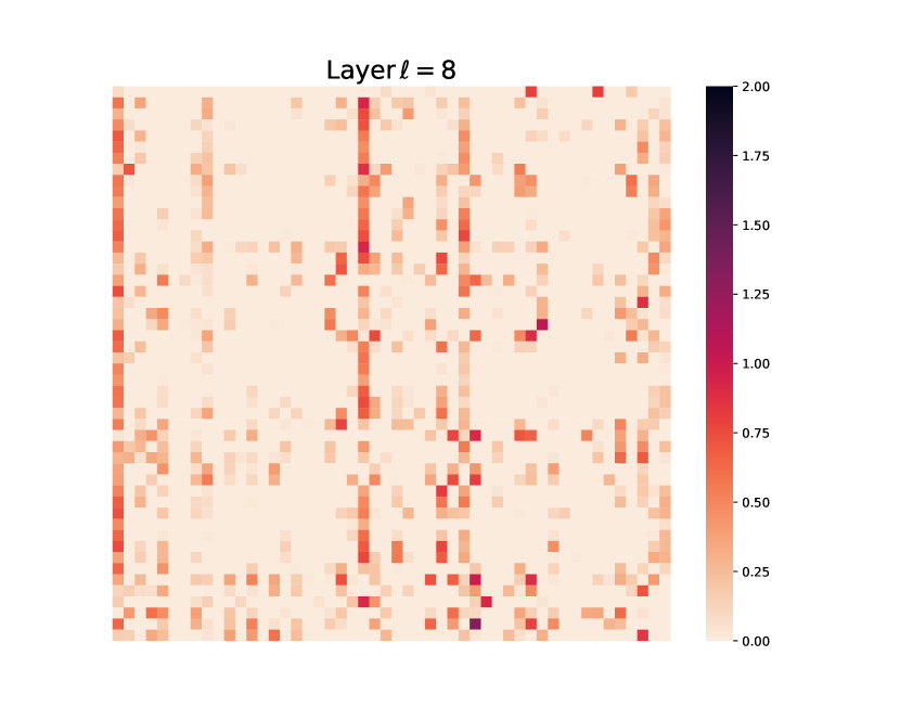
(h) $\ell=8$.

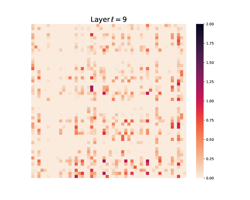
(i) $\ell=9$.

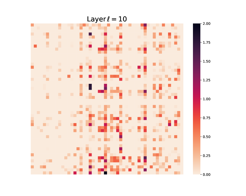
(j) $\ell=10$.

(k) $\ell=11$.

(l) $\ell=12$.

Figure 15: Visualizing layer-wise token $\bm{Z}^{\ell}$ representations at each layer $\ell$. To enhance the visual clarity, we randomly extract a 50$\times$50 sub-matrix from $\bm{Z}^{\ell}$ for display purposes. (Model: crate-Tiny)

Visualizing layer-wise token representations.

To gain a better understanding of the token representations of crate, we visualize the output of each ISTA block at layer $\ell$ in Figure 15. Specifically, we visualize the $\bm{Z}^{\ell+1}$ via heatmap plots. We observe that the output $\bm{Z}^{\ell+1}$ becomes more sparse as the layer increases. Moreover, besides the sparsity, we also find that $\bm{Z}^{\ell+1}$ becomes more structured (i.e., low-rank), which indicates that the set of token representations become closer to linear subspaces, confirming our mental picture of the geometry of each layer (as in Figure 5 and Figure 4).

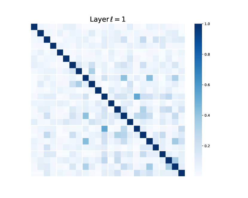
(a) $\ell=1$.

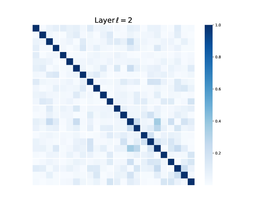
(b) $\ell=2$.

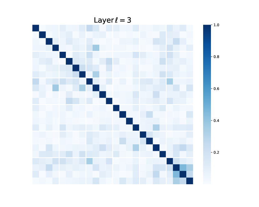
(c) $\ell=3$.

(d) $\ell=4$.

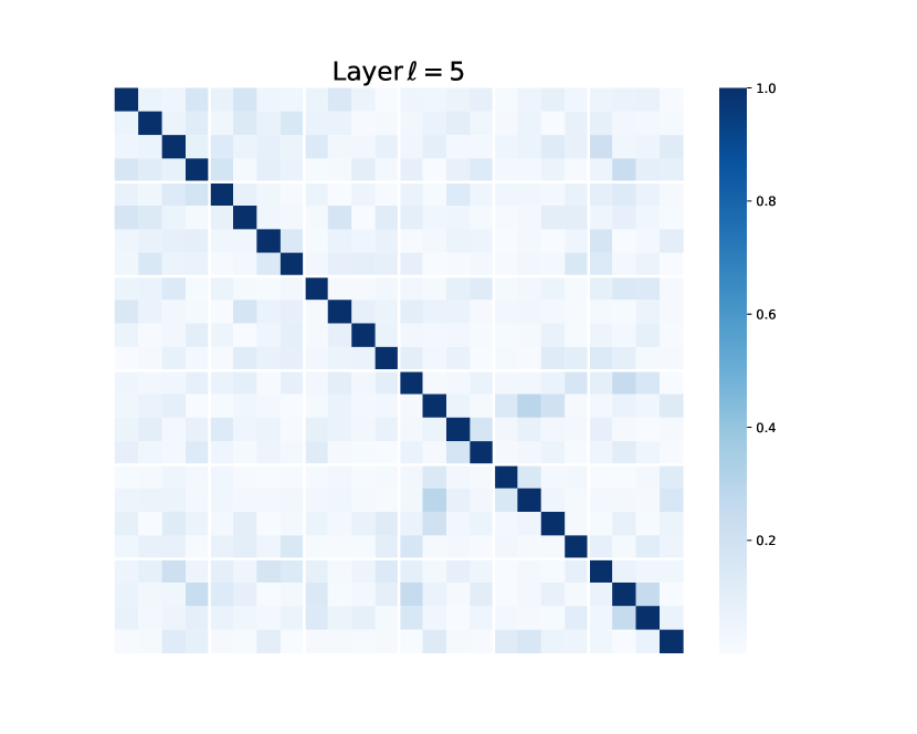
(e) $\ell=5$.

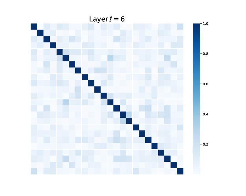
(f) $\ell=6$.

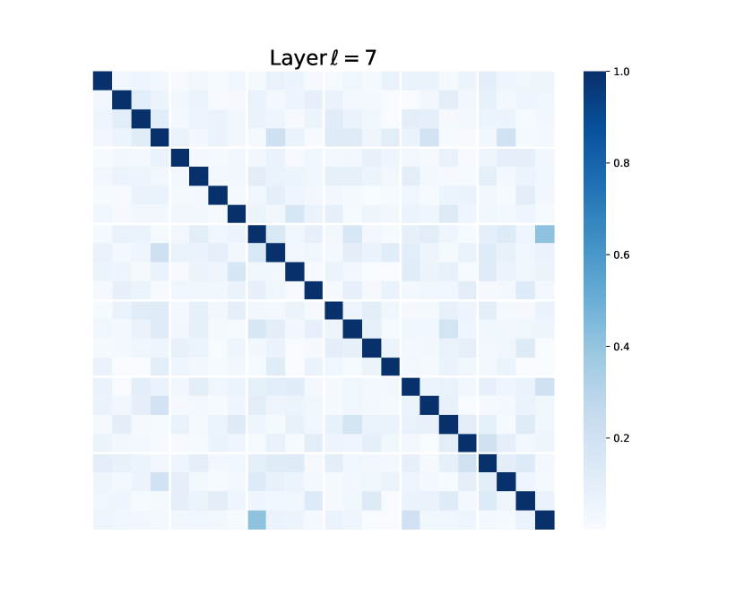
(g) $\ell=7$.

(h) $\ell=8$.

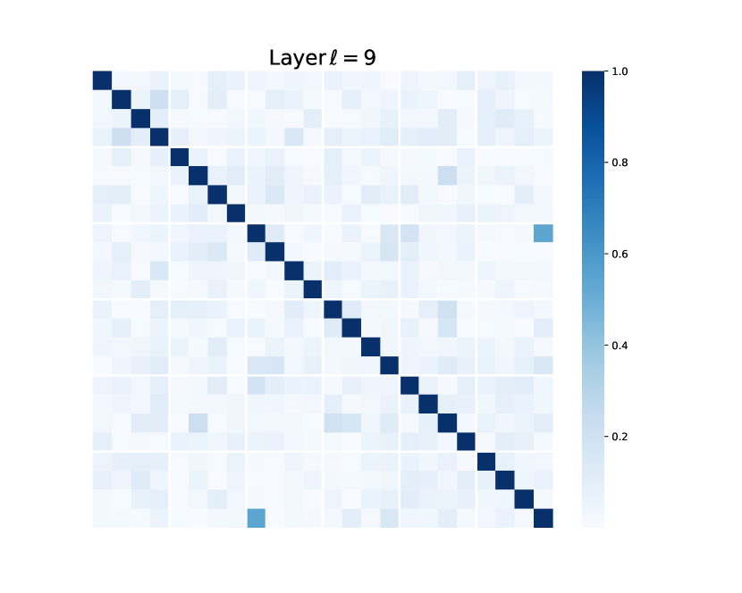
(i) $\ell=9$.

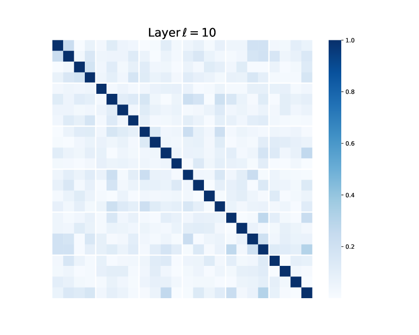
(j) $\ell=10$.

(k) $\ell=11$.

(l) $\ell=12$.

Figure 16: We visualize the $[\bm{U}_{1}^{\ell},\dots,\bm{U}_{K}^{\ell}]^{{}^{\ast}}[\bm{U}_{1}^{\ell},\dots,\bm{U}_{K}^{\ell}]\in\mathbb{R}^{pK\times pK}$ at different layers. The $(i,j)$-th block in each sub-figure corresponds to $(\bm{U}_{i}^{\ell})^{\ast}\bm{U}_{j}^{\ell}$ for $i,j\in[K]$ at a particular layer $\ell$. To enhance the visual clarity, for each subspace $\bm{U}_{i}$, we randomly pick 4 directions for display purposes. (Model: crate-Tiny)

Visualizing layer-wise subspaces in multi-head self-attention.

We now visualize the $\bm{U}_{[K]}^{\ell}$ matrices used in the MSSA block. In Section 2.3, we assumed that $\bm{U}_{[K]}^{\ell}$ were incoherent to capture different “views” of the set of tokens. In Fig. 16, we first normalize the columns in each $\bm{U}_{k}^{\ell}$, then we visualize the $[\bm{U}_{1}^{\ell},\dots,\bm{U}_{K}^{\ell}]^{{}^{\ast}}[\bm{U}_{1}^{\ell},\dots,\bm{U}_{K}^{\ell}]\in\mathbb{R}^{pK\times pK}$. The $(i,j)^{\mathrm{th}}$ block in each sub-figure corresponds to $(\bm{U}_{i}^{\ell})^{\ast}\bm{U}_{j}^{\ell}$ for $i,j\in[K]$ at a particular layer $\ell$. We find that the learned $\bm{U}_{[K]}^{\ell}$ are approximately incoherent, which aligns well with our assumptions. One interesting observation is that the $\bm{U}_{[K]}^{\ell}$ becomes more incoherent when the layer index $\ell$ is larger, which suggests that the token representations are more separable. This mirrors the situation in other popular deep networks (He and Su, 2022a).

4.3 Emergence of Semantic Properties in Learned CRATE Attention Maps

In this subsection, we analyze the attention maps within crate models trained on vision tasks. Previous work (Caron et al., 2021) use the self-attention in vision transformers to study semantic segmentation of the input image. Caron et al. (2021) demonstrated that a specific self-supervised training method, named DINO, can lead to the emergence of segmentation in vision transformers. On the other hand, ViTs trained with supervised learning do not have such properties. In contrast, as we will present in this subsection, we find that the white-box design of crate leads to the emergence of segmentation properties in the network’s self-attention maps, solely through a minimalistic supervised training recipe—the supervised classification training used in vanilla supervised ViTs. We quantify the segmentation properties of crate both qualitatively and quantitatively and compare the results with ViTs. Through extensive evaluations, we find that the self-attention maps in white-box transformers (crate) are much more interpretable than vanilla black-box vision transformers.

4.3.1 Experimental Setup

Model architecture

We utilize the crate model as described in Section 2.5 at sizes -S/8 and -B/8 (that is, crate-Small and crate-Base with patch size $8\times 8$). We similarly adopt the ViT model from Dosovitskiy et al. (2021) using the same scales (-S/8 and -B/8), ensuring consistent configurations between them. Refer to Table 13 for detailed model performance evaluations on classification tasks.

Datasets.

In this subsection, all visual models are trained for classification tasks, using the methodology described in Section 4.1.1, on the complete ImageNet dataset (Deng et al., 2009), commonly referred to as ImageNet-21K. This dataset comprises 14,197,122 images distributed across 21,841 classes. We apply the MaskCut (Wang et al., 2023b) pipeline on the COCO val2017 (Lin et al., 2014), which consists of 5,000 RGB images, and assess our models’ performance for both object detection and instance segmentation tasks. All evaluation procedures are unsupervised, and we do not update the model weights during the detection and segmentation evaluation processes.

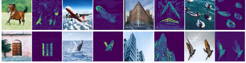
Figure 17: Self-attention maps from a supervised CRATE with $8\times 8$ patches trained using classification. The crate architecture automatically learns to perform object segmentation without a complex self-supervised training recipe or any fine-tuning with segmentation-related annotations. For each image pair, we visualize the original image on the left and the self-attention map of the image on the right.

4.3.2 Measuring the Emergence of Segmentation

Visualizing self-attention maps.

To qualitatively measure the emergence phenomenon, we adopt the attention map approach based on the [CLS] token, which has been widely used as a way to interpret and visualize transformer-like architectures (Abnar and Zuidema, 2020; Caron et al., 2021). Indeed, we use the same methodology as Abnar and Zuidema (2020); Caron et al. (2021), noting that in crate the query-key-value matrices are all the same; a more formal accounting is deferred to Section C.7. The visualization results of self-attention maps are summarized in Figure 17. We observe that the self-attention maps of the crate model correspond to semantic regions in the input image. Our results suggest that the crate model encodes a clear semantic segmentation of each image in the network’s internal representations, which is similar to the self-supervised method DINO (Caron et al., 2021). In contrast, as shown in Figure 25 in the Appendices, the vanilla ViT trained on supervised classification does not exhibit similar segmentation properties.

Object detection and fine-grained segmentation.

To further validate and evaluate the rich semantic information captured by crate, we employ MaskCut (Wang et al., 2023b), a recent effective approach for object detection and segmentation that does not require human annotations. As usual, we provide a more detailed methodological description in Section C.7. This procedure allows us to extract more fine-grained segmentation for an image based on the token representations learned by different methods. In Figure 18, we visualize the fine-grained segmentation produced by MaskCut on features from ViT trained by classification, crate trained by classification as in Section 4.1.1, and crate trained via DINO as in Section 4.1.3, respectively. We compare the segmentation and detection performance in Table 7. Based on these results, we observe that MaskCut on features learned with supervised ViT typically fails to produce good segmentation masks, for example, the first image in Figure 18 and the ViT-S/8 row in Table 7. On the other hand, we notice that, regardless of the training task (supervised or unsupervised), crate is able to capture semantically meaningful boundaries of the main objects in an image. Compared to ViT, crate provides better internal representation tokens for both segmentation and detection.

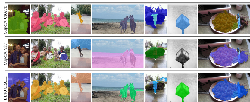
Figure 18: Visualization of segmentation with MaskCut on COCO val2017 (Lin et al., 2014). Top and Bottom Rows: crate architecture clearly detects main objects in the image when trained using either supervised classification technique in Section 4.1.1 or the DINO self-supervised technique in Section 4.1.3  (Caron et al., 2021). Middle Row: Note that compared to crate, ViT trained via classification often fails to detect main objects in the images (columns 2, 3, 4).

Table 7: Object detection and fine-grained segmentation via MaskCut on COCO val2017 (Lin et al., 2014). We consider models with different scales and evaluate the average precision measured by COCO’s official evaluation metric. The first four models are pre-trained with image classification tasks under label supervision; the bottom three models are pre-trained via the DINO self-supervised technique (Caron et al., 2021). crate conclusively performs better than the ViT at detection and segmentation metrics when both are trained using supervised classification.

		Detection			Segmentation
Model	Train	AP50	AP75	AP	AP50	AP75	AP
crate-S/8	Supervised	2.9	1.0	1.1	1.8	0.7	0.8
crate-B/8	Supervised	2.9	1.0	1.3	2.2	0.7	1.0
ViT-S/8	Supervised	0.1	0.1	0.0	0.0	0.0	0.0
ViT-B/8	Supervised	0.8	0.2	0.4	0.7	0.5	0.4
crate-B/8	DINO	3.5	1.1	1.6	2.4	0.5	1.0
ViT-S/8	DINO	5.0	2.0	2.4	4.0	1.3	1.7
ViT-B/8	DINO	5.1	2.3	2.5	4.1	1.3	1.8

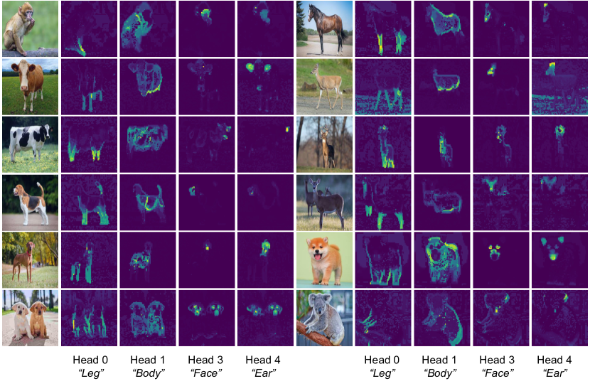
Figure 19: Visualization of semantic heads. We forward a mini-batch of images through a supervised crate and examine the attention maps from all the heads in the penultimate layer. We visualize a selection of attention heads to show that certain heads convey specific semantic meaning, i.e. head 0 $\leftrightarrow$ “Legs”, head 1 $\leftrightarrow$ “Body”, head 3 $\leftrightarrow$ “Face”, head 4 $\leftrightarrow$ “Ear”.

4.3.3 Analysis of Segmentation in CRATE

Segmentation emerges through minimalistic design.

Our empirical results demonstrate that self-supervised learning, as well as the specialized design options in DINO (Caron et al., 2021) (e.g., momentum encoder, student and teacher networks, self-distillation, etc.) are not necessary for the emergence of segmentation. We contend that an equally-promising approach to promote segmentation properties in transformer is to design the transformer architecture with the structure of the input data in mind. This finding of crate represents the first supervised vision model with emergent segmentation properties, and establishes white-box transformers as a promising direction for interpretable data-driven representation learning in foundation models.

Identifying semantic properties of attention heads.

We are interested in capturing the semantic meaning of certain attention heads; this is an important task for interpretability and is already studied for language transformers (Olsson et al., 2022). Intuitively, each head captures certain features of the data. Given a crate model, we first forward an input image (e.g. a horse image as in Figure 19) and select four attention heads which seem to have semantic meaning by manual inspection. After identifying the attention heads, we visualize the self-attention map of these heads on other input images. Interestingly, we find that each of the selected attention heads captures a different part of the object, and even a different semantic meaning. For example, the attention head displayed in the first column of Figure 19 captures the legs of different animals, and the attention head displayed in the last column captures the ears and head. This parsing of the visual input into a part-whole hierarchy has been a fundamental goal of learning-based recognition architectures since deformable part models (Felzenszwalb and Huttenlocher, 2005; Felzenszwalb et al., 2008) and capsule networks (Hinton et al., 2011; Sabour et al., 2017)—strikingly, it emerges from the white-box design of crate within our simple supervised training setup.

5 Conclusions and Open Directions

In this paper, we propose a new theoretical framework that allows us to derive a deep transformer-like network architecture, named crate, as an incremental optimization scheme to learn compressed and sparse representation of the input data, measured by a principled objective for information gain: the sparse rate reduction. The so-derived and learned deep architectures are not only fully mathematically interpretable but also consistent on a layer-by-layer level with their design objective. Despite being arguably the simplest among all possible designs, these networks already demonstrate performance close to seasoned transformers, on large-scale real-world (image or text) datasets and tasks (discriminative and generative), and in supervised, unsupervised, and self-supervised settings.

We believe this work truly helps bridge the gap between theory and practice of deep neural networks, as well as helps unify seemingly separate approaches to learning and representing data distributions through the perspective of data compression. These approaches include, but are not limited to: rate reduction, energy minimization, denoising-diffusion, and transformers. As we have seen, in these approaches, the role of each layer of the associated deep neural networks can be interpreted mathematically as operators to incrementally compress (denoise) and transform the data distribution according to its low-dimensional structures (modeled as Gaussian mixtures). To a large extent, our work suggests that a universal way to effectively and efficiently learn a data distribution with intrinsically low-dimensional structures in a high-dimensional space is through incremental compression, as already stated as a slogan by Wright and Ma (2022):

We compress to learn, and we learn to compress.

This work and the previous work of Chan et al. (2022) together strongly suggest that various deep neural networks are simply means to an end—compression. Different optimization schemes for compression are manifested as different network architectures and operators, e.g. LeNet, LISTA, ResNet, ReduNet, Transformers, which are now elucidated by CRATE.

From a practical standpoint, it is clear that this new framework can now provide us with theoretical guidelines to design and justify new, potentially more powerful, deep architectures for representation learning that are based on more advanced optimization techniques or strategies, instead of the basic gradient-based technique used to construct crate. Also, in this work, we have only used crate to learn deterministic autoencoding models. We believe that this framework can be extended to learn structured representations of the data distribution based on more advanced structured diffusion and denoising. This could potentially lead to more controllable and consistent generative methods, since improving the consistency and efficiency of existing diffusion-based generative models remains a challenging open problem (Song et al., 2023).

Furthermore, as suggested by Dai et al. (2022); Ma et al. (2022), for any system to learn a low-dimensional data distribution autonomously and continuously, one needs to integrate the encoder and decoder not only as an autoencoder but as a closed-loop transcription:

$$\bm{x}\in\mathbb{R}^{D}\xrightarrow{\hskip 5.69054ptf(\bm{x})\hskip 5.69054pt}\bm{z}\in\mathbb{R}^{d}\xrightarrow{\hskip 5.69054ptg(\bm{z})\hskip 5.69054pt}\widehat{\bm{x}}\in\mathbb{R}^{D}\xrightarrow{\hskip 5.69054ptf(\bm{x})\hskip 5.69054pt}\widehat{\bm{z}}\in\mathbb{R}^{d},$$ (89)

which allows the system to correct itself by minimizing the discrepancy between the internal representations $\bm{z}$ of the data and $\widehat{\bm{z}}$ of the generated approximation, without any external help (by human) to compare between the data $\bm{x}$ and $\widehat{\bm{x}}$. So far, the effectiveness of such a closed-loop transcription system has only been demonstrated with black-box deep architectures such as the ResNet (Dai et al., 2022; Tong et al., 2023). It would be possible now to build a closed-loop transcription with purely white-box encoder and decoder designs. This could ultimately enable us to develop complete learning systems that are capable of learning autonomously and continuously an internal data representation that is fully mathematically interpretable, controllable, and eventually self-consistent, or “aligned”, with the true external data distribution. The so-learned representation, just like our acquired memory, can support both discriminative and generative tasks, and serve both recognition and prediction purposes.

Last but not least, we hope that this work provides an alternative viewpoint that may help clarify the ultimate capabilities of modern artificial intelligence (AI) systems, which are typically based on deep networks such as transformers. Just as with all other natural phenomena or technical innovations that were once “black boxes” to people, significant confusion and anxiety is arising in society about the potential or implications of emerging new AI systems, including the recent large language models (LLMs) such as GPT-4 (OpenAI, 2023b), large image generation models such as Midjourney and DALL-E 3 (Betker et al., 2023), and many other multi-modal large language models (MLLMs) (Liu et al., 2023; OpenAI, 2023a). From the perspective of this work, in which we developed a clear understanding of transformer-type learning systems, these large models are unlikely to do anything beyond purely mechanical data compression (encoding) and interpolation (decoding). That is, this work suggests that for these existing large AI models, however magical and mysterious they might appear to be:

Compression is all there is.

This leaves us with a much more profound and challenging question: whether compression alone is all one needs for a system, natural or artificial, to develop general intelligence or even sentience? We believe that compression, employed correctly, is merely the very first step of a long path towards general intelligence.

Acknowledgments and Disclosure of Funding

Yaodong Yu would like to thank Kwan Ho Ryan Chan for the valuable discussions they had regarding visualizing tokens in vision transformers. Yaodong Yu and Yi Ma acknowledge support from the joint Simons Foundation-NSF DMS grant #2031899, the ONR grant N00014-22-1-2102, and Yi Ma also acknowledges support from the University of Hong Kong. Other members of the team were partially supported by NSF 1704458, the Northrop Grumman Mission Systems Research in Applications for Learning Machines (REALM) initiative, NIH NIA 1R01AG067396, and ARO MURI W911NF-17-1-0304.

Appendix

Appendix A Technical Details for Section 2

A.1 Companion to Section 2.3

We now give the derivation of the approximation alluded to in Section 2.3. In the process, we make some simple approximations and technical assumptions. The validity of these assumptions may be explored, and the approximations refined, altogether providing a more complex (and possibly more performant) resulting self-attention like operator. For the sake of technical clarity and simplicity in this work, we make perhaps the simplest possible choices. As a result, we do not claim that our network is optimally designed, but rather that the principles we develop in this work (compression, denoising, sparsification, unrolled optimization) can provide the backbone for far superior and more interpretable network architectures in the future on sundry tasks. As it is, with our straightforward, simple, and interpretable design, we still obtain meaningful conceptual results and very solid empirical performance.

Recall that $\beta=\frac{p}{n\epsilon^{2}}$.

Approximation 9.

Let $\bm{Z}\in\mathbb{R}^{d\times n}$ have unit-norm columns, and $\bm{U}_{[K]}=(\bm{U}_{1},\dots,\bm{U}_{K})$ such that each $\bm{U}_{k}\in\mathbb{R}^{d\times p}$ is an orthogonal matrix, the $(\bm{U}_{k})_{k=1}^{K}$ are incoherent, and the columns of $\bm{Z}$ approximately lie on $\bigcup_{k=1}^{K}\mathrm{Span}(\bm{U}_{k})$. Let $\kappa>0$. Then

$$\bm{Z}-\kappa\nabla_{\bm{Z}}R^{c}(\bm{Z}\mid\bm{U}_{[K]})\approx(1-\kappa\beta)\bm{Z}+\kappa\beta\operatorname{\texttt{MSSA}}(\bm{Z}\mid\bm{U}_{[K]}),$$ (90)

where as in Section 2.3 we have

$$\operatorname{\texttt{SSA}}(\bm{Z}\mid\bm{U}_{k}) =(\bm{U}_{k}^{\ast}\bm{Z})\operatorname{softmax}\left((\bm{U}_{k}^{\ast}\bm{Z})^{\ast}(\bm{U}_{k}^{\ast}\bm{Z})\right),$$ (91)

$$\operatorname{\texttt{MSSA}}(\bm{Z}\mid\bm{U}_{[K]}) =\beta\begin{bmatrix}\bm{U}_{1},\dots,\bm{U}_{K}\end{bmatrix}\begin{bmatrix}\operatorname{\texttt{SSA}}(\bm{Z}\mid\bm{U}_{1})\\ \vdots\\ \operatorname{\texttt{SSA}}(\bm{Z}\mid\bm{U}_{K})\end{bmatrix},$$ (92)

where $\operatorname{softmax}\left(\cdot\right)$ is the softmax operator (applied to each column of an input matrix), i.e.,

$$\operatorname{softmax}\left(\bm{v}\right) =\frac{1}{\sum_{i=1}^{n}e^{v_{i}}}\begin{bmatrix}e^{v_{1}}\\ \vdots\\ e^{v_{n}}\end{bmatrix},$$ (93)

$$\operatorname{softmax}\left(\begin{bmatrix}\bm{v}_{1},\dots,\bm{v}_{K}\end{bmatrix}\right) =\begin{bmatrix}\operatorname{softmax}\left(\bm{v}_{1}\right),\dots,\operatorname{softmax}\left(\bm{v}_{K}\right)\end{bmatrix}.$$ (94)

Proof.

According to 31, the gradient $\nabla_{\bm{Z}}{R}^{c}(\bm{Z}\mid\bm{U}_{[K]})$ is

$$\nabla_{\bm{Z}}{R}^{c}(\bm{Z}\mid\bm{U}_{[K]})=\beta\sum_{k=1}^{K}\bm{U}_{k}\bm{U}_{k}^{\ast}\bm{Z}\left(\bm{I}+\beta(\bm{U}_{k}^{\ast}\bm{Z})^{\ast}(\bm{U}_{k}^{\ast}\bm{Z})\right)^{-1}.$$ (95)

Notice that according to (Chan et al., 2022), the gradient is precisely the residual of a ridge regression for each (projected) token $\bm{U}_{k}^{\ast}\bm{z}_{i}$ using other projected tokens $\bm{U}_{k}^{\ast}\bm{z}_{j}$ as the regressors, hence being the residual of an auto-regression.

However, as we have seen in the work of ReduNet (Chan et al., 2022), computing the inverse $\left(\bm{I}+\beta(\bm{U}_{k}^{*}\bm{Z})^{*}(\bm{U}_{k}^{*}\bm{Z})\right)^{-1}$ can be expensive. Hence for computational efficiency, we may approximate it with the first order term of its von Neumann expansion:

$$\nabla_{\bm{Z}}{R}^{c}(\bm{Z}\mid\bm{U}_{[K]}) =\beta\sum_{k=1}^{K}\bm{U}_{k}\bm{U}_{k}^{*}\bm{Z}\Big{(}{\bm{I}+\beta(\bm{U}_{k}^{*}\bm{Z})^{*}(\bm{U}_{k}^{*}\bm{Z})}\Big{)}^{-1}$$ (96)

$$\approx\beta\sum_{k=1}^{K}\bm{U}_{k}\bm{U}_{k}^{*}\bm{Z}\Big{(}{\bm{I}-\beta(\bm{U}_{k}^{*}\bm{Z})^{*}(\bm{U}_{k}^{*}\bm{Z})}\Big{)}$$ (97)

$$=\beta\sum_{k=1}^{K}\bm{U}_{k}\Big{(}{\bm{U}^{*}_{k}\bm{Z}-\beta\bm{U}^{*}_{k}\bm{Z}[(\bm{U}_{k}^{\ast}\bm{Z})^{\ast}(\bm{U}_{k}^{\ast}\bm{Z})]}\Big{)}$$ (98)

Notice that the term $(\bm{U}_{k}^{\ast}\bm{Z})^{\ast}(\bm{U}_{k}^{\ast}\bm{Z})$ is the auto-correlation among the projected tokens. As the tokens $\bm{Z}$ may be from different subspaces, we would prefer to use only tokens that belong to the same subspace to regress and compress themselves. Hence we may convert the above correlation term into a subspace-membership indicator with a softmax operation, whence (98) becomes

$$\nabla_{\bm{Z}}{R}^{c}(\bm{Z}\mid\bm{U}_{[K]}) \approx \beta\sum_{k=1}^{K}\bm{U}_{k}\Big{(}{\bm{U}^{*}_{k}\bm{Z}-\beta\bm{U}^{*}_{k}\bm{Z}[(\bm{U}_{k}^{\ast}\bm{Z})^{\ast}(\bm{U}_{k}^{\ast}\bm{Z})]}\Big{)}$$ (99)

$$\approx \beta\sum_{k=1}^{K}\bm{U}_{k}\bm{U}_{k}^{*}\bm{Z}-\beta^{2}\sum_{k=1}^{K}\bm{U}_{k}\Big{(}\bm{U}_{k}^{*}\bm{Z}\operatorname{softmax}\left((\bm{U}_{k}^{\ast}\bm{Z})^{\ast}(\bm{U}_{k}^{\ast}\bm{Z})\right)\Big{)}$$ (100)

Then, we can rewrite the above approximation to the gradient of $R^{c}$ as:

$$\nabla_{\bm{Z}}{R}^{c}(\bm{Z}\mid\bm{U}_{[K]}) \approx\beta\sum_{k=1}^{K}\bm{U}_{k}\bm{U}_{k}^{*}\bm{Z}-\beta^{2}\sum_{k=1}^{K}\bm{U}_{k}\left(\bm{U}_{k}^{*}\bm{Z}\operatorname{softmax}\left((\bm{U}_{k}^{\ast}\bm{Z})^{\ast}(\bm{U}_{k}^{\ast}\bm{Z})\right)\right)$$ (101)

$$=\beta\sum_{k=1}^{K}\bm{U}_{k}\bm{U}_{k}^{*}\bm{Z}-\beta^{2}\sum_{k=1}^{K}\bm{U}_{k}\operatorname{\texttt{SSA}}(\bm{Z}\mid\bm{U}_{k})$$ (102)

$$=\beta\underbrace{\left(\sum_{k=1}^{K}\bm{U}_{k}\bm{U}_{k}^{*}\right)\bm{Z}}_{\approx\bm{Z}}-\beta^{2}\begin{bmatrix}\bm{U}_{1},\cdots,\bm{U}_{K}\end{bmatrix}\begin{bmatrix}\operatorname{\texttt{SSA}}(\bm{Z}\mid\bm{U}_{1})\\ \vdots\\ \operatorname{\texttt{SSA}}(\bm{Z}\mid\bm{U}_{K})\end{bmatrix}$$ (103)

$$\approx\beta\bm{Z}-\beta^{2}\begin{bmatrix}\bm{U}_{1},\cdots,\bm{U}_{K}\end{bmatrix}\begin{bmatrix}\operatorname{\texttt{SSA}}(\bm{Z}\mid\bm{U}_{1})\\ \vdots\\ \operatorname{\texttt{SSA}}(\bm{Z}\mid\bm{U}_{K})\end{bmatrix}$$ (104)

$$=\beta\bm{Z}-\beta\operatorname{\texttt{MSSA}}(\bm{Z}\mid\bm{U}_{[K]})$$ (105)

Thus the gradient descent step with learning rate $\kappa>0$ gives

$$\bm{Z}-\kappa\nabla_{\bm{Z}}R^{c}(\bm{Z}\mid\bm{U}_{[K]})\approx(1-\kappa\beta)\bm{Z}+\kappa\beta\operatorname{\texttt{MSSA}}(\bm{Z}\mid\bm{U}_{[K]}).$$ (106)

∎

A.2 Companion to Section 2.4

In the main text Section 2.4, our connection between the second step of the alternating minimization and the LASSO optimization was high-level and heuristic. In some sense, the choice to pose the minimization step as a LASSO was a simple, reliable, and interpretable choice which works well in practice, but is nonetheless not backed up by rigorous theoretical justification. In the following subsection, we provide a mathematical justification for a reformulation of the minimization step using a majorization-minimization framework. We further show that the associated unrolled optimization step bears a strong resemblance to the ISTA step. This confirms our earlier discussion — we took the simplest possible choice in designing crate, but by more rigorous derivation we can uncover alternative operators which nonetheless have the same conceptual function and may perform better in practice.

Assumptions.

In this section, we present a rigorous optimization analysis of an incremental minimization approach to the objective 25. We will show that under two simplifying assumptions, namely

1. The columns of $\bm{Z}^{\ell+1/2}$ are normalized, in the sense that $\operatorname{diag}((\bm{Z}^{\ell+1/2})^{\ast}\bm{Z}^{\ell+1/2})=\bm{1}$;

2. We have $d\geq n$, and the columns of $\bm{Z}^{\ell+1/2}$ are orthogonal, so that $(\bm{Z}^{\ell+1/2})^{\ast}\bm{Z}^{\ell+1/2}=\bm{I}$.

the approach leads to an update iteration that is equal to a slightly simplified version of the ISTA block 42. We see this as a justification for our derivation in Section 2.4, which obtained the ISTA block by introducing an additional simplifying assumption on the distribution of the data at layer $\ell$.

Analysis.

Following 41, we will consider the natural relaxation of the $\ell^{0}$ “norm” to the $\ell^{1}$ norm, and incorporate a nonnegativity constraint. Consider the objective

$$\varphi(\bm{Z})=\lambda\lVert\bm{Z}\rVert_{1}+\chi_{\{\bm{Z}\geq\mathbf{0}\}}(\bm{Z})-\underbrace{\frac{1}{2}\log\det\left(\bm{I}+\alpha\bm{Z}^{\ast}\bm{Z}\right)}_{R(\bm{Z})},$$ (107)

where $\bm{Z}\in\mathbb{R}^{d\times N}$ and $\alpha=d/(n\varepsilon^{2})$, and $\chi_{\{\bm{Z}\geq\mathbf{0}\}}$ denotes the characteristic function for the set of elementwise-nonnegative matrices $\bm{Z}$. As in Section A.1, we calculate

$$\nabla_{\bm{Z}}R(\bm{Z})=\alpha\bm{Z}\left(\bm{I}+\alpha\bm{Z}^{\ast}\bm{Z}\right)^{-1}.$$ (108)

We consider an incremental optimization scheme for the highly nonlinear and nonconvex objective $\varphi$. Following Section 2.3, we optimize locally at a “post-compression” iterate $\bm{Z}^{\ell+1/2}$. We follow the standard proximal majorize-minimize framework (Wright and Ma, 2022) for incremental/local optimization: this begins with the second-order Taylor expansion for the smooth part of $\varphi$ in a neighborhood of the current iterate $\bm{Z}^{\ell+1/2}$:

$$\begin{split}R(\bm{Z})=R(\bm{Z}^{\ell+1/2})&+\left\langle\nabla_{\bm{Z}}R(\bm{Z}^{\ell+1/2}),\bm{Z}-\bm{Z}^{\ell+1/2}\right\rangle\\ &+\int_{0}^{1}(1-t)\left\langle\bm{Z}-\bm{Z}^{\ell+1/2},\nabla^{2}R(\bm{Z}_{t})\left(\bm{Z}-\bm{Z}^{\ell+1/2}\right)\right\rangle\ \mathrm{d}t,\end{split}$$ (109)

where for any $\bm{Z}\in\mathbb{R}^{d\times n}$, $\bm{Z}_{t}=t\bm{Z}^{\ell+1/2}+(1-t)\bm{Z}$. The proximal majorization-minimization approach alternates two steps to minimize $\varphi$:

1. First, use assumptions on $\bm{Z}^{\ell+1/2}$ to derive an upper bound on the operator norm of the Hessian $\nabla^{2}R(\bm{Z})$ over the effective domain of the optimization problem. We will write $L$ for this (uniform) upper bound. This yields a quadratic upper bound for the smooth part of the objective $\varphi$.

2. Then, alternately minimize the smooth part of the quadratic upper bound as a function of $\bm{Z}$, and take a proximal step on the nonsmooth part. It can be shown (Wright and Ma, 2022) that corresponds to the iteration

   $$\bm{Z}^{+}={\operatorname{prox}}_{\frac{\lambda}{L}(\lVert\>\cdot\>\rVert_{1}+\chi_{\{\bm{Z}\geq\mathbf{0}\}})}\left(\bm{Z}+\frac{1}{L}\nabla_{\bm{Z}}R(\bm{Z})\right)$$ (110)

   In the alternating minimization setting of this paper for optimizing 15, we only take one such step, starting at $\bm{Z}^{\ell+1/2}$.

We will instantiate this program below, showing quantitative error bounds related to our assumptions above as necessary. Rather than directly applying the iteration 110, we will derive it below under our aforementioned assumptions.

Starting at 109, our first task is to upper bound the quadratic residual. This corresponds to estimating

$$\left\langle\bm{Z}-\bm{Z}^{\ell+1/2},\nabla^{2}R(\bm{Z}_{t})\left(\bm{Z}-\bm{Z}^{\ell+1/2}\right)\right\rangle$$ (111)

$$\qquad\leq\sup_{t\in[0,1]}\left\lVert\nabla^{2}R(\bm{Z}_{t})\right\rVert_{\ell^{2}\to\ell^{2}}\left\lVert\bm{Z}-\bm{Z}^{\ell+1/2}\right\rVert_{F}^{2}$$ (112)

with Cauchy-Schwarz. Using Lemma 10, we can estimate the operator norm term in the previous bound in terms of properties of $\bm{Z}^{\ell+1/2}$. We need to bound

$$\alpha\sup_{\lVert\bm{\Delta}\rVert_{F}\leq 1}\left\lVert\left(\bm{\Delta}-\alpha\bm{Z}_{t}(\bm{I}+\alpha\bm{Z}_{t}^{\ast}\bm{Z}_{t})^{-1}(\bm{Z}_{t}^{\ast}\bm{\Delta}+\bm{\Delta}^{\ast}\bm{Z}_{t})\right)(\bm{I}+\alpha\bm{Z}_{t}^{\ast}\bm{Z}_{t})^{-1}\right\rVert_{F},$$ (113)

and Lemma 11 gives that this term is no larger than $9\alpha/4$ for any $\bm{Z}$ and any $t$. With this estimate and 109, we have a quadratic upper bound for $-R(\bm{Z})$:

$$-R(\bm{Z})\leq-R(\bm{Z}^{\ell+1/2})+\left\langle-\nabla_{\bm{Z}}R(\bm{Z}^{\ell+1/2}),\bm{Z}-\bm{Z}^{\ell+1/2}\right\rangle\\ +\frac{9\alpha}{8}\left\lVert\bm{Z}-\bm{Z}^{\ell+1/2}\right\rVert_{F}^{2}.$$ (114)

Meanwhile, by our assumptions above, we have

$$-\nabla_{\bm{Z}}R(\bm{Z}^{\ell+1/2})=-\alpha\bm{Z}^{\ell+1/2}\left(\bm{I}+\alpha\bm{I}\right)^{-1}=-\frac{\alpha}{1+\alpha}\bm{Z}^{\ell+1/2}.$$ (115)

We now minimize the preceding quadratic upper bound as a function of $\bm{Z}$. Differentiating, the minimizer $\bm{Z}_{\mathrm{opt}}$ is calculated as

$$\bm{Z}_{\mathrm{opt}}=\left(1+\frac{4}{9(1+\alpha)}\right)\bm{Z}^{\ell+1/2},$$ (116)

and it is well-known that the proximal operator of the sum of $\chi_{\{\bm{Z}\geq\mathbf{0}\}}$ and $\lambda\lVert\>\cdot\>\rVert_{1}$ is simply the one-sided soft-thresholding operator (Wright and Ma, 2022)

$${\operatorname{prox}}_{\chi_{\{\bm{Z}\geq\mathbf{0}\}}+\lambda\lVert\>\cdot\>\rVert_{1}}\left(\bm{Z}\right)=\max\{\bm{Z}-\lambda\mathbf{1},\mathbf{0}\},$$ (117)

where the maximum is applied elementwise. As in Section 2.4, we may write this elementwise maximum simply as $\operatorname{ReLU}$. Thus, one step of proximal majorization-minimization under our simplifying assumptions takes the form

$$\bm{Z}^{\ell+1}=\operatorname{ReLU}\left(\left(1+\frac{4}{9(1+\alpha)}\right)\bm{Z}^{\ell+1/2}-\frac{4\lambda}{9\alpha}\mathbf{1}\right).$$ (118)

Finally, we point out one additional elaboration which introduces the dictionary $\bm{D}$ that appears in the ISTA block in Section 2.4. Notice that for any orthogonal $\bm{D}$, one has $R(\bm{D}\bm{Z})=R(\bm{Z})$ for every $\bm{Z}$. This symmetry implies equivariance properties of $\nabla_{\bm{Z}}R(\bm{Z})$ and $\nabla^{2}_{\bm{Z}}R(\bm{Z})$: for every $\bm{Z}$ and every $\bm{\Delta}$ and every orthogonal $\bm{D}$,

$$\bm{D}\nabla_{\bm{Z}}R(\bm{Z}) =\nabla_{\bm{Z}}R(\bm{D}\bm{Z}),$$ (119)

$$\langle\bm{D}\bm{\Delta},\nabla^{2}_{\bm{Z}}R(\bm{Z})\left(\bm{D}\bm{\Delta}\right)\rangle =\langle\bm{\Delta},\nabla^{2}_{\bm{Z}}R(\bm{D}\bm{Z})\left(\bm{\Delta}\right)\rangle.$$ (120)

Hence the quadratic Taylor expansion 109 can be written equivalently as

$$\begin{split}R(\bm{Z})=R(\bm{D}^{\ast}\bm{Z}^{\ell+1/2})&+\left\langle\nabla_{\bm{Z}}R(\bm{D}^{\ast}\bm{Z}^{\ell+1/2}),\bm{Z}-\bm{Z}^{\ell+1/2}\right\rangle\\ &+\int_{0}^{1}(1-t)\left\langle\bm{Z}-\bm{Z}^{\ell+1/2},\nabla^{2}R(\bm{D}^{\ast}\bm{Z}_{t})\left(\bm{Z}-\bm{Z}^{\ell+1/2}\right)\right\rangle\ \mathrm{d}t,\end{split}$$ (121)

for any orthogonal $\bm{D}$. The significance of this is that we have obtained an expression equivalent to 109, but with $\bm{Z}^{\ell+1/2}$ replaced by $\bm{D}^{\ast}\bm{Z}^{\ell+1/2}$; moreover, because our approximation arguments above are not affected by left-multiplication of $\bm{Z}^{\ell+1/2}$ by an orthogonal matrix (this operation does not change the norms of the columns of $\bm{Z}^{\ell+1/2}$, or their correlations, and hence the matrix’s incoherence), we can apply exactly the same line of reasoning above to obtain that an equivalent proximal majorization-minimization iteration is given by

$$\bm{Z}^{\ell+1}=\operatorname{ReLU}\left(\left(1+\frac{4}{9(1+\alpha)}\right)\bm{D}^{\ast}\bm{Z}^{\ell+1/2}-\frac{4\lambda}{9\alpha}\mathbf{1}\right),$$ (122)

for any orthogonal dictionary $\bm{D}$. This gives an update quite similar to the ISTA block 42 in the case where the dictionary used in Section 2.4 is orthogonal, but without a skip connection.

We thus obtain a natural white-box version of this part of the architecture, along with the natural interpretation that its purpose is to sparsify the compressed tokens $\bm{Z}^{\ell+1/2}$ in a (learnable) dictionary, which accords with recent empirical studies (Li et al., 2023b).

Other architectures?

As we mentioned at the start of this section, the preceding derivation is performed in the most elementary possible setting in order to demonstrate the majorization-minimization approach for layer design. More precise approximations or assumptions may lead to superior layer designs that better optimize the target objective 15 (and in particular 25). We mention two here:

1. Beyond exactly-incoherent features: our derivations above assumed that the incoming representations $\bm{Z}^{\ell+1/2}$ were already maximal for the expansion term $R$ in 25. It is desirable to obtain a ‘perturbative’ derivation, which applies in cases where $\bm{Z}^{\ell+1/2}$ is not fully orthogonal, but instead near-orthogonal, in particular incoherent (Wright and Ma, 2022). The derivations above can be adapted to this setting; the perturbation bounds become slightly more delicate, and the ultimate layer 122 changes to involve additional normalization.

2. Beyond orthogonal dictionaries: The symmetries of the expansion term $R$ in 25 may be followed to lead to a pair of dictionaries $\bm{D}$ and $\bm{D}^{\prime}$ and an objective that sparsifies $\bm{D}\bm{Z}\bm{D}^{\prime}$. This type of transformation is suggestive of popular architectures that mix over tokens (Tolstikhin et al., 2021; Trockman et al., 2023), however we consider the simpler form $\bm{D}\bm{Z}$ in this work. In addition, we have focused for simplicity on orthogonal dictionaries $\bm{D}$; as in the previous bullet, one may consider in a similar way dictionaries $\bm{D}$ which are complete and near-orthogonal. Adapting the derivation to overcomplete dictionaries is an interesting future direction that we expect to improve the scalability of crate; one avenue to achieve this could be increasing the number of projections $\bm{U}_{[K]}$ and their embedding dimensions.

A.2.1 Auxiliary Lemmas

Lemma 10.

Consider the function

$$R(\bm{Z})=\frac{1}{2}\log\det\left(\bm{I}+\alpha\bm{Z}^{\ast}\bm{Z}\right),$$ (123)

where $\alpha>0$ is a constant. Then we have

$$\nabla_{\bm{Z}}R(\bm{Z})=\alpha\bm{Z}\left(\bm{I}+\alpha\bm{Z}^{\ast}\bm{Z}\right)^{-1},$$ (124)

and the Hessian operator $\nabla_{\bm{Z}}^{2}R(\bm{Z})\colon\mathbb{R}^{d\times N}\to\mathbb{R}^{d\times N}$ satisfies that for any $\bm{\Delta}\in\mathbb{R}^{d\times N}$,

$$\nabla^{2}_{\bm{Z}}R(\bm{Z})\left(\bm{\Delta}\right)$$ (125)

$$=\alpha\bm{\Delta}\left(\bm{I}+\alpha\bm{Z}^{\ast}\bm{Z}\right)^{-1}-\alpha^{2}\bm{Z}\left(\bm{I}+\alpha\bm{Z}^{\ast}\bm{Z}\right)^{-1}\left(\bm{Z}^{\ast}\bm{\Delta}+\bm{\Delta}^{\ast}\bm{Z}\right)\left(\bm{I}+\alpha\bm{Z}^{\ast}\bm{Z}\right)^{-1}.$$ (126)

Proof.

The gradient calculation follows from (Yu et al., 2020), for example. For the Hessian, we use the usual approach to calculating derivatives: if $\bm{\Delta}$ is any matrix with the same shape as $\bm{Z}$ and $t>0$,

$$\nabla_{\bm{Z}}^{2}R(\bm{Z})\left(\bm{\Delta}\right)={\left.\kern-1.2pt\frac{\partial}{\partial t}\vphantom{\big{|}}\right|_{t=0}}\left[t\mapsto\nabla_{\bm{Z}}R(\bm{Z}+t\bm{\Delta})\right],$$ (127)

valid since $R$ is smooth. We have

$$\nabla_{\bm{Z}}R(\bm{Z}+t\bm{\Delta})$$

$$= \alpha(\bm{Z}+t\bm{\Delta})\left(\bm{I}+\alpha(\bm{Z}+t\bm{\Delta})^{\ast}(\bm{Z}+t\bm{\Delta})\right)^{-1}$$

$$= \alpha(\bm{Z}+t\bm{\Delta})\left(\bm{I}+\alpha\bm{Z}^{\ast}\bm{Z}+\alpha t\left[\bm{Z}^{\ast}\bm{\Delta}+\bm{\Delta}^{\ast}\bm{Z}+t\bm{\Delta}^{\ast}\bm{\Delta}\right]\right)^{-1}$$

$$= \alpha(\bm{Z}+t\bm{\Delta})\left(\bm{I}+\alpha t\left(\bm{I}+\alpha\bm{Z}^{\ast}\bm{Z}\right)^{-1}\left[\bm{Z}^{\ast}\bm{\Delta}+\bm{\Delta}^{\ast}\bm{Z}+t\bm{\Delta}^{\ast}\bm{\Delta}\right]\right)^{-1}\left(\bm{I}+\alpha\bm{Z}^{\ast}\bm{Z}\right)^{-1}$$

$$= \alpha(\bm{Z}+t\bm{\Delta})\left(\sum_{k=0}^{\infty}(-\alpha t)^{k}\left(\left(\bm{I}+\alpha\bm{Z}^{\ast}\bm{Z}\right)^{-1}\left[\bm{Z}^{\ast}\bm{\Delta}+\bm{\Delta}^{\ast}\bm{Z}+t\bm{\Delta}^{\ast}\bm{\Delta}\right]\right)^{k}\right)\left(\bm{I}+\alpha\bm{Z}^{\ast}\bm{Z}\right)^{-1},$$

where in the fourth line we require that $t$ is sufficiently close to $0$ in order to invoke the Neumann series. First, notice that the term involving $\bm{\Delta}^{\ast}\bm{\Delta}$ does not play a role in the final expression: after we differentiate with respect to $t$ and take a limit $t\to 0$, terms arising due to differentiation of $t\mapsto t\bm{\Delta}^{\ast}\bm{\Delta}$ go to zero, because whenever the summation index $k>0$ we have a term $(-\alpha t)^{k}$ that goes to zero as $t\to 0$. We thus obtain with the product rule

$${\left.\kern-1.2pt\frac{\partial}{\partial t}\vphantom{\big{|}}\right|_{t=0}}\left[t\mapsto\nabla_{\bm{Z}}R(\bm{Z}+t\bm{\Delta})\right]$$ (128)

$$=\,\, \alpha\bm{\Delta}\left(\bm{I}+\alpha\bm{Z}^{\ast}\bm{Z}\right)^{-1}-\alpha^{2}\bm{Z}\left(\bm{I}+\alpha\bm{Z}^{\ast}\bm{Z}\right)^{-1}\left(\bm{Z}^{\ast}\bm{\Delta}+\bm{\Delta}^{\ast}\bm{Z}\right)\left(\bm{I}+\alpha\bm{Z}^{\ast}\bm{Z}\right)^{-1}.$$ (129)

∎

Lemma 11.

One has

$$\sup_{\lVert\bm{\Delta}\rVert_{F}\leq 1}\left\lVert\left(\bm{\Delta}-\alpha\bm{Z}_{t}(\bm{I}+\alpha\bm{Z}_{t}^{\ast}\bm{Z}_{t})^{-1}(\bm{Z}_{t}^{\ast}\bm{\Delta}+\bm{\Delta}^{\ast}\bm{Z}_{t})\right)(\bm{I}+\alpha\bm{Z}_{t}^{\ast}\bm{Z}_{t})^{-1}\right\rVert_{F}\leq\frac{9}{4}.$$ (130)

Proof.

Fix $\bm{\Delta}$ satisfying $\lVert\bm{\Delta}\rVert_{F}\leq 1$. By the triangle inequality,

$$\left\lVert\left(\bm{\Delta}-\alpha\bm{Z}_{t}(\bm{I}+\alpha\bm{Z}_{t}^{\ast}\bm{Z}_{t})^{-1}(\bm{Z}_{t}^{\ast}\bm{\Delta}+\bm{\Delta}^{\ast}\bm{Z}_{t})\right)(\bm{I}+\alpha\bm{Z}_{t}^{\ast}\bm{Z}_{t})^{-1}\right\rVert_{F}$$ (131)

$$\leq\left\lVert\bm{\Delta}(\bm{I}+\alpha\bm{Z}_{t}^{\ast}\bm{Z}_{t})^{-1}\right\rVert_{F}+\alpha\left\lVert\bm{Z}_{t}(\bm{I}+\alpha\bm{Z}_{t}^{\ast}\bm{Z}_{t})^{-1}(\bm{Z}_{t}^{\ast}\bm{\Delta}+\bm{\Delta}^{\ast}\bm{Z}_{t})(\bm{I}+\alpha\bm{Z}_{t}^{\ast}\bm{Z}_{t})^{-1}\right\rVert_{F}.$$ (132)

For the first term, we note that

$$\left\lVert\bm{\Delta}(\bm{I}+\alpha\bm{Z}_{t}^{\ast}\bm{Z}_{t})^{-1}\right\rVert_{F}=\left\lVert\left((\bm{I}+\alpha\bm{Z}_{t}^{\ast}\bm{Z}_{t})^{-1}\otimes\bm{I}\right)\operatorname{vec}(\bm{\Delta})\right\rVert_{F},$$ (133)

and since $(\bm{I}+\alpha\bm{Z}_{t}^{\ast}\bm{Z}_{t})^{-1}\preceq\bm{I}$, we obtain from Cauchy-Schwarz

$$\left\lVert\bm{\Delta}(\bm{I}+\alpha\bm{Z}_{t}^{\ast}\bm{Z}_{t})^{-1}\right\rVert_{F}\leq\lVert\bm{\Delta}\rVert_{F}.$$ (134)

We can use a similar idea to control the second term. We have from the triangle inequality

$$\left\lVert\bm{Z}_{t}(\bm{I}+\alpha\bm{Z}_{t}^{\ast}\bm{Z}_{t})^{-1}(\bm{Z}_{t}^{\ast}\bm{\Delta}+\bm{\Delta}^{\ast}\bm{Z}_{t})(\bm{I}+\alpha\bm{Z}_{t}^{\ast}\bm{Z}_{t})^{-1}\right\rVert_{F}$$ (135)

$$\quad\leq\left\lVert\bm{Z}_{t}(\bm{I}+\alpha\bm{Z}_{t}^{\ast}\bm{Z}_{t})^{-1}\bm{Z}_{t}^{\ast}\bm{\Delta}(\bm{I}+\alpha\bm{Z}_{t}^{\ast}\bm{Z}_{t})^{-1}\right\rVert_{F}$$ (136)

$$\qquad+\left\lVert(\bm{I}+\alpha\bm{Z}_{t}^{\ast}\bm{Z}_{t})^{-1}\bm{Z}_{t}^{\ast}\bm{\Delta}(\bm{I}+\alpha\bm{Z}_{t}^{\ast}\bm{Z}_{t})^{-1}\bm{Z}_{t}^{\ast}\right\rVert_{F}.$$ (137)

For the first term, we have

$$\left\lVert\bm{Z}_{t}(\bm{I}+\alpha\bm{Z}_{t}^{\ast}\bm{Z}_{t})^{-1}\bm{Z}_{t}^{\ast}\bm{\Delta}(\bm{I}+\alpha\bm{Z}_{t}^{\ast}\bm{Z}_{t})^{-1}\right\rVert_{F}$$ (138)

$$\quad=\left\lVert\left((\bm{I}+\alpha\bm{Z}_{t}^{\ast}\bm{Z}_{t})^{-1}\otimes\bm{Z}_{t}(\bm{I}+\alpha\bm{Z}_{t}^{\ast}\bm{Z}_{t})^{-1}\bm{Z}_{t}^{\ast}\right)\operatorname{vec}(\bm{\Delta})\right\rVert_{F}$$ (139)

$$\quad\leq\sigma_{\max}\left((\bm{I}+\alpha\bm{Z}_{t}^{\ast}\bm{Z}_{t})^{-1}\right)\sigma_{\max}\left(\bm{Z}_{t}(\bm{I}+\alpha\bm{Z}_{t}^{\ast}\bm{Z}_{t})^{-1}\bm{Z}_{t}^{\ast}\right)\lVert\bm{\Delta}\rVert_{F}$$ (140)

$$\quad\leq\frac{1}{\alpha}\lVert\bm{\Delta}\rVert_{F}.$$ (141)

The last estimate follows from a computation using the SVD of $\bm{Z}_{t}$. Meanwhile, we have for the second term by a similar argument (using the fact that the singular values of $\bm{A}$ and $\bm{A}^{\ast}$ are identical for any matrix $\bm{A}$)

$$\left\lVert(\bm{I}+\alpha\bm{Z}_{t}^{\ast}\bm{Z}_{t})^{-1}\bm{Z}_{t}^{\ast}\bm{\Delta}(\bm{I}+\alpha\bm{Z}_{t}^{\ast}\bm{Z}_{t})^{-1}\bm{Z}_{t}^{\ast}\right\rVert_{F} \leq\sigma_{\max}\left((\bm{I}+\alpha\bm{Z}_{t}^{\ast}\bm{Z}_{t})^{-1}\bm{Z}_{t}^{\ast}\right)^{2}\lVert\bm{\Delta}\rVert_{F}$$ (142)

$$\leq\frac{1}{4\alpha}\lVert\bm{\Delta}\rVert_{F},$$ (143)

where once again the estimate follows from a computation involving the SVD of $\bm{Z}_{t}$ (together with the fact that the function $\sigma\mapsto\sigma/(1+\alpha\sigma^{2})$ is bounded on $\sigma\geq 0$ by $1/(2\sqrt{\alpha})$). Putting it together, we have obtained

$$\left\lVert\left(\bm{\Delta}-\alpha\bm{Z}_{t}(\bm{I}+\alpha\bm{Z}_{t}^{\ast}\bm{Z}_{t})^{-1}(\bm{Z}_{t}^{\ast}\bm{\Delta}+\bm{\Delta}^{\ast}\bm{Z}_{t})\right)(\bm{I}+\alpha\bm{Z}_{t}^{\ast}\bm{Z}_{t})^{-1}\right\rVert_{F}\leq\frac{9}{4}\lVert\bm{\Delta}\rVert_{F},$$ (144)

which gives the claim after taking suprema.

∎

Appendix B Technical Details for Section 3

B.1 An Overview of Diffusion Processes

In this section, we give an overview of the basics of time-reversible Itô diffusion processes, the mathematical foundation for diffusion models. This is to make this paper more self-contained by providing knowledge about general diffusion processes that we will apply to our special models. The coverage adapts that of Millet et al. (1989b); Song et al. (2021b); Karras et al. (2022).

Consider a generic Itô diffusion process $(\bm{z}(t))_{t\in[0,T]}$, where $\bm{z}(t)$ is an $\mathbb{R}^{m}$-valued random variable, given by the SDE

$$\odif{\bm{z}(t)}=b(\bm{z}(t),t)\odif{t}+\Sigma(\bm{z}(t),t)\odif{\bm{w}(t)},\qquad\bm{z}(0)\sim P,\qquad\forall t\in[0,T]$$ (145)

where $\bm{w}$ is a Brownian motion and $P$ is some probability measure on $\mathbb{R}^{m}$ (in this case representing the data distribution). Here the drift coefficient $b\colon\mathbb{R}^{m}\times\mathbb{R}\to\mathbb{R}^{m}$ and diffusion coefficient $\Sigma\colon\mathbb{R}^{m}\times\mathbb{R}\to\mathbb{R}^{m\times m}$ are functions. To make sense of 145 and also verify the existence of strong (i.e., pathwise well-defined) solutions, we need some regularity on them, and we choose the following assumption:

1. $b$ and $\Sigma$ have some spatial smoothness and do not grow too fast, i.e., there is a constant $K\geq 0$ such that for all $\bm{x},\widetilde{\bm{z}}\in\mathbb{R}^{m}$ we have

   $$\sup_{t\in[0,T]}\left[\lVert\Sigma(\bm{x},t)-\Sigma(\widetilde{\bm{z}},t)\rVert_{F}+\lVert b(\bm{x},t)-b(\widetilde{\bm{z}},t)\rVert_{2}\right]\leq K\lVert\bm{x}-\widetilde{\bm{z}}\rVert_{2}$$ (146)

   $$\sup_{t\in[0,T]}\left[\lVert\Sigma(\bm{x},t)\rVert_{F}+\lVert b(\bm{x},t)\rVert_{2}\right]\leq K(1+\lVert\bm{x}\rVert_{2}).$$ (147)

In general, $\bm{z}(t)$ may not have a density w.r.t. the Lebesgue measure on $\mathbb{R}^{m}$. For example, suppose that $P$ is supported on some low-dimensional linear subspace (or even a Dirac delta measure), and take $\Sigma$ to be the orthoprojector onto this subspace. Then $\bm{z}(t)$ will be supported on this subspace for all $t$ and thus not have a density w.r.t. the Lebesgue measure. Thus, when further discussing processes of the type 145, we make the following assumption

1. $\bm{z}(t)$ has a probability density function $p(\cdot,t)$ for all $t>0$.

   This is guaranteed by either of the following conditions (Millet et al., 1989b):

   1. $b$ and $\Sigma$ are differentiable in $(\bm{x},t)$ and have Hölder-continuous derivatives, and $P$ has a density w.r.t. the Lebesgue measure;

   2. The event

      $$\{\text{$\operatorname{rank}(\Sigma(\bm{z}(s),s))=m$ for all $s$ in some neighborhood of $0$}\}$$ (148)

      happens $P$-almost surely.

Define $\Psi\colon\mathbb{R}^{m}\times\mathbb{R}\to\mathbb{R}^{m\times m}$ by

$$\Psi(\bm{x},t)\doteq\Sigma(\bm{x},t)\Sigma(\bm{x},t)^{\ast}.$$ (149)

To discuss time-reversibility, we also need the following local integrability condition, which is another measure of sharp growth of the coefficients (or precisely their derivatives):

1. The functions $(\bm{x},t)\mapsto\nabla_{\bm{x}}\cdot(\Psi(\bm{x},t)p(\bm{x},t))$ are integrable on sets of the form $D\times[t_{0},1]$ for $t_{0}>0$ and $D$ a bounded measurable subset of $\mathbb{R}^{m}$:

   $$\int_{t_{0}}^{1}\int_{D}\lVert\nabla_{\bm{x}}\cdot(\Psi(\bm{x},t)p(\bm{x},t))\rVert_{2}\odif{\bm{x}}\odif{t}<\infty.$$ (150)

To write the notation out more explicitly,

$$\nabla_{\bm{x}}\cdot(\Psi(\bm{x},t)p(\bm{x},t))=\begin{bmatrix}\nabla_{\bm{x}}\cdot(\Psi^{1}(\bm{x},t)p(\bm{x},t))\\ \vdots\\ \nabla_{\bm{x}}\cdot(\Psi^{m}(\bm{x},t)p(\bm{x},t))\end{bmatrix}$$ (151)

where $$\nabla_{\bm{x}}\cdot(\Psi^{i}(\bm{x},t)p(\bm{x},t))=\sum_{j=1}^{m}\pdv*{[\Psi^{ij}(\bm{x},t)p(\bm{x},t)]}{x_{j}}$$ (152)

where $\Psi^{i}$ is the $i^{\mathrm{th}}$ row of $\Psi$ transposed to a column, and $\Psi^{ij}$ is the $(i,j)^{\mathrm{th}}$ entry of $\Psi$. Note that Millet et al. (1989b) phrases this in terms of an local integrability condition on each $\lvert\nabla_{\bm{x}}\cdot(\Psi^{i}(\bm{x},t)p(\bm{x},t))\rvert$, which would naturally give a local integrability condition on $\lVert\nabla_{\bm{x}}\cdot(\Psi(\bm{x},t)p(\bm{x},t))\rVert_{\infty}$. However, all norms on $\mathbb{R}^{m}$ are equivalent, and so this leads to a local integrability condition for $\lVert\nabla_{x}\cdot(\Psi(\bm{x},t)p(\bm{x},t))\rVert_{2}$ as produced. Note that the assumptions do not guarantee that the involved derivatives exist, in which case they are taken in the distributional (e.g., weak) sense, whence they should exist (Millet et al., 1989b).

Under assumptions A1—A3, Millet et al. (1989b) guarantees the existence of another process $(\widetilde{\bm{z}}(t))_{t\in[0,T]}$ such that the laws of $\bm{z}(t)$ and $\widetilde{\bm{z}}(T-t)$ are the same for all $t\in[0,T]$. This process $(\widetilde{\bm{z}}(t))_{t\in[0,T]}$ is called the time reversal of $(\bm{z}(t))_{t\in[0,T]}$, and is shown to have law given by

$$\odif{\widetilde{\bm{z}}(t)}=b^{\leftarrow}(\widetilde{\bm{z}}(t),t)\odif{t}+\Sigma^{\leftarrow}(\widetilde{\bm{z}}(t),t)\odif{\bm{w}^{\leftarrow}(t)},\qquad\widetilde{\bm{z}}(0)\sim p(\cdot,T),\qquad\forall t\in[0,T]$$ (153)

where $\bm{w}^{\leftarrow}(t)$ is an independent Brownian motion and

$$b^{\leftarrow}(\bm{x},t) =-b(\bm{x},T-t)+\frac{\nabla_{\bm{x}}\cdot[\Psi(\bm{x},T-t)p(\bm{x},T-t)]}{p(\bm{x},T-t)}$$ (154)

$$=-b(\bm{x},T-t)+\nabla_{\bm{x}}\cdot\Psi(\bm{x},T-t)+\Psi(\bm{x},T-t)[\nabla_{\bm{x}}\log p(\bm{x},T-t)],$$ (155)

$$\Sigma^{\leftarrow}(\bm{x},t) =\Sigma(\bm{x},T-t).$$ (156)

We would next like to develop an ODE which transports the probability mass $P$ in the same way as 145 — namely, find another process $(\mkern 1.5mu\overline{\mkern-1.5mu\bm{z}\mkern-1.5mu}\mkern 1.5mu(t))_{t\in[0,T]}$ which has deterministic dynamics, yet has the same law as $(\bm{z}(t))_{t\in[0,T]}$. Song et al. (2021b) looks at the Fokker-Planck equations (which can be defined, at least in a weak sense, under assumptions A1–A2) and manipulates them to get the following dynamics for $\mkern 1.5mu\overline{\mkern-1.5mu\bm{z}\mkern-1.5mu}\mkern 1.5mu(t)$:

$$\odif{\mkern 1.5mu\overline{\mkern-1.5mu\bm{z}\mkern-1.5mu}\mkern 1.5mu(t)} =\mkern 1.5mu\overline{\mkern-1.5mub\mkern-1.5mu}\mkern 1.5mu(\mkern 1.5mu\overline{\mkern-1.5mu\bm{z}\mkern-1.5mu}\mkern 1.5mu(t),t)\odif{t},\qquad\mkern 1.5mu\overline{\mkern-1.5mu\bm{z}\mkern-1.5mu}\mkern 1.5mu(0)\sim P,\qquad\forall t\in[0,T],$$ (157)

$$\text{where}\qquad\mkern 1.5mu\overline{\mkern-1.5mub\mkern-1.5mu}\mkern 1.5mu(\bm{x},t) =b(\bm{x},t)-\frac{1}{2}\cdot\frac{\nabla_{\bm{x}}\cdot[\Psi(\bm{x},t)p(\bm{x},t)]}{p(\bm{x},t)}$$ (158)

$$=b(\bm{x},t)-\frac{1}{2}\nabla_{\bm{x}}\cdot\Psi(\bm{x},t)-\frac{1}{2}\Psi(\bm{x},t)[\nabla_{x}\log p(\bm{x},t)].$$ (159)

Now to get a similar process for $\widetilde{\bm{z}}(t)$, namely a process $(\mkern 1.5mu\overline{\mkern-1.5mu\widetilde{\bm{z}}\mkern-1.5mu}\mkern 1.5mu(t))_{t\in[0,T]}$ which evolves deterministically yet has the same law as $(\widetilde{\bm{z}}(t))_{t\in[0,T]}$, we may either take the time reversal of 157 or apply the Fokker-Planck method to 153, in both cases obtaining the same dynamics:

$$\small\odif{\mkern 1.5mu\overline{\mkern-1.5mu\widetilde{\bm{z}}\mkern-1.5mu}\mkern 1.5mu(t)} =\mkern 1.5mu\overline{\mkern-1.5mub\mkern-1.5mu}\mkern 1.5mu^{\leftarrow}(\mkern 1.5mu\overline{\mkern-1.5mu\widetilde{\bm{z}}\mkern-1.5mu}\mkern 1.5mu(t),t)\odif{t},\qquad\mkern 1.5mu\overline{\mkern-1.5mu\widetilde{\bm{z}}\mkern-1.5mu}\mkern 1.5mu(0)\sim p(\cdot,T),\qquad\forall t\in[0,T],$$ (160)

where

$$\mkern 1.5mu\overline{\mkern-1.5mub\mkern-1.5mu}\mkern 1.5mu^{\leftarrow}(\bm{x},t) =-\mkern 1.5mu\overline{\mkern-1.5mub\mkern-1.5mu}\mkern 1.5mu(\bm{x},T-t)$$ (161)

$$=-b(\bm{x},T-t)+\frac{1}{2}\cdot\frac{\nabla_{\bm{x}}\cdot[\Psi(\bm{x},T-t)p(\bm{x},T-t)]}{p(\bm{x},T-t)}$$ (162)

$$=-b(\bm{x},t)+\frac{1}{2}\nabla_{\bm{x}}\cdot\Psi(\bm{x},T-t)+\frac{1}{2}\Psi(\bm{x},T-t)[\nabla_{\bm{x}}\log p(\bm{x},T-t)].$$ (163)

The quantity $\nabla_{\bm{x}}\log p(\bm{x},t)$ is of central importance; it is denoted the score at time $t$, and we use the notation $s(\bm{x},t)\doteq\nabla_{x}\log p(\bm{x},t)$ for it. With this substitution, we have the following dynamics for our four processes:

$$\odif{\bm{z}(t)} =b(\bm{z}(t),t)\odif{t}+\Sigma(\bm{z}(t),t)\odif{\bm{w}(t)},\quad\bm{z}(0)\sim P$$ (164)

$$\odif{\widetilde{\bm{z}}(t)} =[-b(\widetilde{\bm{z}}(t),T-t)+\nabla_{\bm{x}}\cdot\Psi(\widetilde{\bm{z}}(t),T-t)+\Psi(\widetilde{\bm{z}}(t),T-t)s(\widetilde{\bm{z}}(t),T-t)]\odif{t}$$ (165)

$$\qquad+\Sigma(\widetilde{\bm{z}}(t),T-t)\odif{\bm{w}^{\leftarrow}(t)},\quad\widetilde{\bm{z}}(0)\sim p(\cdot,T)$$ (166)

$$\odif{\mkern 1.5mu\overline{\mkern-1.5mu\bm{z}\mkern-1.5mu}\mkern 1.5mu(t)} =\left[b(\mkern 1.5mu\overline{\mkern-1.5mu\bm{z}\mkern-1.5mu}\mkern 1.5mu(t),t)-\frac{1}{2}\nabla_{\bm{x}}\cdot\Psi(\mkern 1.5mu\overline{\mkern-1.5mu\bm{z}\mkern-1.5mu}\mkern 1.5mu(t),t)-\frac{1}{2}\Psi(\mkern 1.5mu\overline{\mkern-1.5mu\bm{z}\mkern-1.5mu}\mkern 1.5mu(t),t)s(\mkern 1.5mu\overline{\mkern-1.5mu\bm{z}\mkern-1.5mu}\mkern 1.5mu(t),t)\right]\odif{t},\quad\mkern 1.5mu\overline{\mkern-1.5mu\bm{z}\mkern-1.5mu}\mkern 1.5mu(0)\sim P$$ (167)

$$\odif{\mkern 1.5mu\overline{\mkern-1.5mu\widetilde{\bm{z}}\mkern-1.5mu}\mkern 1.5mu(t)} =\bigg{[}-b(\mkern 1.5mu\overline{\mkern-1.5mu\widetilde{\bm{z}}\mkern-1.5mu}\mkern 1.5mu(t),T-t)+\frac{1}{2}\nabla_{\bm{x}}\cdot\Psi(\mkern 1.5mu\overline{\mkern-1.5mu\widetilde{\bm{z}}\mkern-1.5mu}\mkern 1.5mu(t),T-t)$$ (168)

$$\qquad+\frac{1}{2}\Psi(\mkern 1.5mu\overline{\mkern-1.5mu\widetilde{\bm{z}}\mkern-1.5mu}\mkern 1.5mu(t),T-t)s(\mkern 1.5mu\overline{\mkern-1.5mu\widetilde{\bm{z}}\mkern-1.5mu}\mkern 1.5mu(t),T-t)\bigg{]}\odif{t},\quad\mkern 1.5mu\overline{\mkern-1.5mu\widetilde{\bm{z}}\mkern-1.5mu}\mkern 1.5mu(0)\sim p(\cdot,T).$$ (169)

In practice, one fits an estimator for $s(\cdot,\cdot)$ and estimates $p(\cdot,T)$ and runs a discretization of either 153 or 160 to sample approximately from $P$. One common instantiation used in diffusion models (Karras et al., 2022) is the so-called variance-exploding diffusion process, which has the coefficient settings

$$b(\bm{x},t)=0,\qquad\Sigma(\bm{x},t)=\sqrt{2}\bm{I}$$ (170)

which implies that

$$\Psi(\bm{x},t)=2\bm{I}.$$ (171)

This means that the four specified processes are of the form

$$\odif{\bm{z}(t)} =\sqrt{2}\odif{\bm{w}(t)},\quad\bm{z}(0)\sim P$$ (172)

$$\odif{\widetilde{\bm{z}}(t)} =s(\widetilde{\bm{z}}(t),T-t)\odif{t}+\sqrt{2}\odif{\bm{w}^{\leftarrow}(t)},\quad\widetilde{\bm{z}}(0)\sim p(\cdot,T)$$ (173)

$$\odif{\mkern 1.5mu\overline{\mkern-1.5mu\bm{z}\mkern-1.5mu}\mkern 1.5mu(t)} =s(\mkern 1.5mu\overline{\mkern-1.5mu\bm{z}\mkern-1.5mu}\mkern 1.5mu(t),t)\odif{t},\quad\mkern 1.5mu\overline{\mkern-1.5mu\bm{z}\mkern-1.5mu}\mkern 1.5mu(0)\sim P$$ (174)

$$\odif{\mkern 1.5mu\overline{\mkern-1.5mu\widetilde{\bm{z}}\mkern-1.5mu}\mkern 1.5mu(t)} =-s(\mkern 1.5mu\overline{\mkern-1.5mu\widetilde{\bm{z}}\mkern-1.5mu}\mkern 1.5mu(t),T-t),\quad\mkern 1.5mu\overline{\mkern-1.5mu\widetilde{\bm{z}}\mkern-1.5mu}\mkern 1.5mu(0)\sim p(\cdot,T).$$ (175)

Notice that the determinstic flows are actually gradient flows on the score, which concretely reveals a connection between sampling and optimization, and thus between diffusion models (precisely those which use the probability flow ODE to sample) and unrolled optimization networks.

In this context, we can also establish the connection between diffusion networks and iterative denoising. In the variance-exploding setting, we have

$$\bm{z}(t)\sim\mathcal{N}(\bm{z}(0),2t\bm{I}),$$ (176)

which can be easily computed using results from, e.g., Särkkä and Solin (2019). Thus $\bm{z}(t)$ is a noisy version of $\bm{z}(0)$, with noise level increasing monotonically with $t$, and sampling $\bm{z}(0)$ from $\bm{z}(t)$ conceptually removes this noise. Concretely, Tweedie’s formula (Efron, 2011b) says that the optimal denoising function $\mathbb{E}[\bm{z}(0)\nonscript\>|\allowbreak\nonscript\>\mathopen{}\bm{z}(t)]$ has a simple form in terms of the score function:

$$\mathbb{E}[\bm{z}(0)\nonscript\>|\allowbreak\nonscript\>\mathopen{}\bm{z}(t)]=\bm{z}(t)+2t\cdot s(\bm{z}(t),t).$$ (177)

In other words, the score function $s$ points from the current iterate $\bm{z}(t)$ to the value of the optimal denoising function, so it is a negative multiple of the conditionally-expected noise. Following the score by (stochastic) gradient flow or its discretization is thus equivalent to iterative denoising.

B.2 Companion to Section 3.1

Here we produce the approximation result alluded to in Section 3.1. To simplify the proofs, we use the following notation correspondences: $\bm{x}\mapsto\bm{z}^{\ell}$, $\bm{z}\mapsto\bm{z}_{\natural}^{\ell}$, and $\sigma\mapsto\sigma^{\ell}$.

Approximation 12.

Suppose that $\bm{z}$ follows the low-dimensional Gaussian mixture model 10 with respect to subspaces $\bm{U}_{[K]}$, so that $\bm{x}=\bm{z}+\sigma\bm{w}$, where $\bm{w}$ is a standard Gaussian vector independent of $\bm{z}$, follows 11. That is, for some random index $s\sim\pi$ where $\pi$ is a distribution on $[K]$ and $s$ is chosen independently of all other randomness, we have

$$\bm{z}=\bm{U}_{s}\bm{\alpha},$$ (178)

where $\bm{\alpha}$ is a zero-mean Gaussian vector with diagonal covariance $\bm{\Lambda}$. For each $k\in[K]$, define

$$\bm{\Sigma}_{i}\doteq\operatorname{Cov}[\bm{z}\mid s=k]=\bm{U}_{k}\bm{\Lambda}\bm{U}_{k}^{\ast}.$$ (179)

Assume (for the sake of normalization) that

$$\frac{\pi_{i}}{\sqrt{\det(\bm{\Sigma}_{i}+\sigma^{2}\bm{I})}}=\frac{\pi_{j}}{\sqrt{\det(\bm{\Sigma}_{j}+\sigma^{2}\bm{I})}},\qquad\text{for all}\ 1\leq i\leq j\leq K.$$ (180)

Then we have

$$\mathbb{E}[\bm{z}\mid\bm{x}]\approx\begin{bmatrix}\bm{U}_{1},\dots,\bm{U}_{K}\end{bmatrix}\left[\operatorname{diag}\left(\operatorname{softmax}\left(\frac{1}{2\sigma^{2}}\begin{bmatrix}\lVert\bm{U}_{1}^{\ast}\bm{x}\rVert_{2}^{2}\\ \vdots\\ \lVert\bm{U}_{K}^{\ast}\bm{x}\rVert_{2}^{2}\end{bmatrix}\right)\right)\otimes\bm{I}_{p}\right]\begin{bmatrix}\bm{U}_{1}^{\ast}\bm{x}\\ \vdots\\ \bm{U}_{K}^{\ast}\bm{x}\end{bmatrix},$$ (181)

where $\otimes$ denotes the Kronecker product, i.e., the block matrix defined by

$$\bm{A}\otimes\bm{B}=\begin{bmatrix}A_{11}\bm{B}&\cdots&A_{1n}\bm{B}\\ \vdots&\ddots&\vdots\\ A_{m1}\bm{B}&\cdots&A_{mn}\bm{B}\end{bmatrix}.$$ (182)

Proof.

Define $\bm{M}_{k}\doteq(\bm{\Sigma}_{k}+\sigma^{2}\bm{I})^{-1/2}$. From Proposition 14, we have

$$\nabla_{\bm{x}}\log q(\bm{x}) =-\sum_{k=1}^{K}\bm{e}_{k}^{\ast}\operatorname{softmax}\left(-\frac{1}{2}\begin{bmatrix}\lVert\bm{M}_{1}^{\ast}\bm{x}\rVert_{2}^{2}\\ \vdots\\ \lVert\bm{M}_{K}^{\ast}\bm{x}\rVert_{2}^{2}\end{bmatrix}\right)\bm{M}_{k}\bm{M}_{k}^{\ast}\bm{x}$$ (183)

$$=-\sum_{k=1}^{K}\bm{e}_{k}^{\ast}\operatorname{softmax}\left(-\frac{1}{2\sigma^{2}}\begin{bmatrix}\lVert\sigma\bm{M}_{1}^{\ast}\bm{x}\rVert_{2}^{2}\\ \vdots\\ \lVert\sigma\bm{M}_{K}^{\ast}\bm{x}\rVert_{2}^{2}\end{bmatrix}\right)\bm{M}_{k}\bm{M}_{k}^{\ast}\bm{x}$$ (184)

$$=-\sum_{k=1}^{K}\bm{e}_{k}^{\ast}\operatorname{softmax}\left(\frac{1}{2\sigma^{2}}\begin{bmatrix}\lVert\bm{x}\rVert_{2}^{2}-\lVert\sigma\bm{M}_{1}^{\ast}\bm{x}\rVert_{2}^{2}\\ \vdots\\ \lVert\bm{x}\rVert_{2}^{2}-\lVert\sigma\bm{M}_{K}^{\ast}\bm{x}\rVert_{2}^{2}\end{bmatrix}\right)\bm{M}_{k}\bm{M}_{k}^{\ast}\bm{x}.$$ (185)

Now define $\bm{P}_{k}\doteq\bm{I}_{d}-\sigma\bm{M}_{k}$, and let $\bm{U}_{k}^{\perp}\in\mathbb{R}^{d\times(d-p)}$ be an orthogonal complement of $\bm{U}_{k}$. Then we have

$$\bm{P}_{k} =\bm{I}_{d}-\sigma\bm{M}_{k}$$ (186)

$$=\bm{I}_{d}-\sigma\left(\bm{\Sigma}_{k}+\sigma^{2}\bm{I}_{d}\right)^{-1/2}$$ (187)

$$=\bm{I}_{d}-\sigma\left(\begin{bmatrix}\bm{U}_{k}&\bm{U}_{k}^{\perp}\end{bmatrix}\begin{bmatrix}\bm{\Lambda}&\mathbf{0}\\ \mathbf{0}&\mathbf{0}\end{bmatrix}\begin{bmatrix}\bm{U}_{k}^{\ast}\\ (\bm{U}_{k}^{\perp})^{\ast}\end{bmatrix}+\sigma^{2}\bm{I}_{d}\right)^{-1/2}$$ (188)

$$=\bm{I}_{d}-\sigma\left(\begin{bmatrix}\bm{U}_{k}&\bm{U}_{k}^{\perp}\end{bmatrix}\begin{bmatrix}\bm{\Lambda}+\sigma^{2}\bm{I}_{p}&\mathbf{0}\\ \mathbf{0}&\sigma^{2}\bm{I}_{d-p}\end{bmatrix}\begin{bmatrix}\bm{U}_{k}^{\ast}\\ (\bm{U}_{k}^{\perp})^{\ast}\end{bmatrix}\right)^{-1/2}$$ (189)

$$=\bm{I}_{d}-\begin{bmatrix}\bm{U}_{k}&\bm{U}_{k}^{\perp}\end{bmatrix}\begin{bmatrix}\sigma(\bm{\Lambda}+\sigma^{2}\bm{I}_{p})^{-1/2}&\mathbf{0}\\ \mathbf{0}&\sigma\cdot(\sigma^{2})^{-1/2}\bm{I}_{d-p}\end{bmatrix}\begin{bmatrix}\bm{U}_{k}^{\ast}\\ (\bm{U}_{k}^{\perp})^{\ast}\end{bmatrix}$$ (190)

$$=\bm{I}_{d}-\begin{bmatrix}\bm{U}_{k}&\bm{U}_{k}^{\perp}\end{bmatrix}\begin{bmatrix}(\sigma^{-2}\bm{\Lambda}+\bm{I}_{p})^{-1/2}&\mathbf{0}\\ \mathbf{0}&\bm{I}_{d-p}\end{bmatrix}\begin{bmatrix}\bm{U}_{k}^{\ast}\\ (\bm{U}_{k}^{\perp})^{\ast}\end{bmatrix}$$ (191)

$$=\begin{bmatrix}\bm{U}_{k}&\bm{U}_{k}^{\perp}\end{bmatrix}\begin{bmatrix}\bm{I}_{p}-(\sigma^{-2}\bm{\Lambda}+\bm{I}_{p})^{-1/2}&\mathbf{0}\\ \mathbf{0}&\mathbf{0}\end{bmatrix}\begin{bmatrix}\bm{U}_{k}^{\ast}\\ (\bm{U}_{k}^{\perp})^{\ast}\end{bmatrix}$$ (192)

$$\approx\begin{bmatrix}\bm{U}_{k}&\bm{U}_{k}^{\perp}\end{bmatrix}\begin{bmatrix}\bm{I}_{p}&\mathbf{0}\\ \mathbf{0}&\mathbf{0}\end{bmatrix}\begin{bmatrix}\bm{U}_{k}^{\ast}\\ (\bm{U}_{k}^{\perp})^{\ast}\end{bmatrix}$$ (193)

$$=\bm{U}_{k}\bm{U}_{k}^{\ast}.$$ (194)

Thus $\bm{P}_{k}$ is approximately a projection when $\sigma$ is small. Under this algebraic relation, we have

$$\nabla_{\bm{x}}\log q(\bm{x})$$ (195)

$$=-\sum_{k=1}^{K}\bm{e}_{k}^{\ast}\operatorname{softmax}\left(\frac{1}{2\sigma^{2}}\begin{bmatrix}\lVert\bm{x}\rVert_{2}^{2}-\lVert\sigma\bm{M}_{1}^{\ast}\bm{x}\rVert_{2}^{2}\\ \vdots\\ \lVert\bm{x}\rVert_{2}^{2}-\lVert\sigma\bm{M}_{K}^{\ast}\bm{x}\rVert_{2}^{2}\end{bmatrix}\right)\bm{M}_{k}\bm{M}_{k}^{\ast}\bm{x}$$ (196)

$$=-\frac{1}{\sigma^{2}}\sum_{k=1}^{K}\bm{e}_{k}^{\ast}\operatorname{softmax}\left(\frac{1}{2\sigma^{2}}\begin{bmatrix}\lVert\bm{x}\rVert_{2}^{2}-\lVert(\bm{I}_{d}-\bm{P}_{1})^{\ast}\bm{x}\rVert_{2}^{2}\\ \vdots\\ \lVert\bm{x}\rVert_{2}^{2}-\lVert(\bm{I}_{d}-\bm{P}_{K})^{\ast}\bm{x}\rVert_{2}^{2}\end{bmatrix}\right)(\bm{I}_{d}-\bm{P}_{k})(\bm{I}_{d}-\bm{P}_{k})^{\ast}\bm{x}$$ (197)

$$\approx-\frac{1}{\sigma^{2}}\sum_{k=1}^{K}\bm{e}_{k}^{\ast}\operatorname{softmax}\left(\frac{1}{2\sigma^{2}}\begin{bmatrix}\lVert\bm{P}_{1}^{\ast}\bm{x}\rVert_{2}^{2}\\ \vdots\\ \lVert\bm{P}_{K}^{\ast}\bm{x}\rVert_{2}^{2}\end{bmatrix}\right)(\bm{I}_{d}-\bm{P}_{k})(\bm{I}_{d}-\bm{P}_{k})^{\ast}\bm{x}$$ (198)

$$\approx-\frac{1}{\sigma^{2}}\sum_{k=1}^{K}\bm{e}_{k}^{\ast}\operatorname{softmax}\left(\frac{1}{2\sigma^{2}}\begin{bmatrix}\lVert\bm{P}_{1}^{\ast}\bm{x}\rVert_{2}^{2}\\ \vdots\\ \lVert\bm{P}_{K}^{\ast}\bm{x}\rVert_{2}^{2}\end{bmatrix}\right)(\bm{I}_{d}-\bm{P}_{k})^{*}\bm{x}$$ (199)

$$=-\frac{\bm{x}}{\sigma^{2}}\sum_{k=1}^{K}\bm{e}_{k}^{\ast}\operatorname{softmax}\left(\frac{1}{2\sigma^{2}}\begin{bmatrix}\lVert\bm{P}_{1}^{\ast}\bm{x}\rVert_{2}^{2}\\ \vdots\\ \lVert\bm{P}_{K}^{\ast}\bm{x}\rVert_{2}^{2}\end{bmatrix}\right)+\frac{1}{\sigma^{2}}\sum_{k=1}^{K}\bm{e}_{k}^{\ast}\operatorname{softmax}\left(\frac{1}{2\sigma^{2}}\begin{bmatrix}\lVert\bm{P}_{1}^{\ast}\bm{x}\rVert_{2}^{2}\\ \vdots\\ \lVert\bm{P}_{K}^{\ast}\bm{x}\rVert_{2}^{2}\end{bmatrix}\right)\bm{P}_{k}^{\ast}\bm{x}$$ (200)

$$=-\frac{1}{\sigma^{2}}\bm{x}+\frac{1}{\sigma^{2}}\sum_{k=1}^{K}\bm{e}_{k}^{\ast}\operatorname{softmax}\left(\frac{1}{2\sigma^{2}}\begin{bmatrix}\lVert\bm{P}_{1}^{\ast}\bm{x}\rVert_{2}^{2}\\ \vdots\\ \lVert\bm{P}_{K}^{\ast}\bm{x}\rVert_{2}^{2}\end{bmatrix}\right)\bm{P}_{k}^{\ast}\bm{x}$$ (201)

$$\approx-\frac{1}{\sigma^{2}}\bm{x}+\frac{1}{\sigma^{2}}\sum_{k=1}^{K}\bm{e}_{k}^{\ast}\operatorname{softmax}\left(\frac{1}{2\sigma^{2}}\begin{bmatrix}\lVert\bm{U}_{1}^{\ast}\bm{x}\rVert_{2}^{2}\\ \vdots\\ \lVert\bm{U}_{K}^{\ast}\bm{x}\rVert_{2}^{2}\end{bmatrix}\right)\bm{U}_{k}\bm{U}_{k}^{\ast}\bm{x}$$ (202)

$$=-\frac{1}{\sigma^{2}}\bm{x}+\frac{1}{\sigma^{2}}\begin{bmatrix}\bm{U}_{1},\cdots,\bm{U}_{K}\end{bmatrix}\left[\operatorname{diag}\left(\operatorname{softmax}\left(\frac{1}{2\sigma^{2}}\begin{bmatrix}\lVert\bm{U}_{1}^{\ast}\bm{x}\rVert_{2}^{2}\\ \vdots\\ \lVert\bm{U}_{K}^{\ast}\bm{x}\rVert_{2}^{2}\end{bmatrix}\right)\right)\otimes\bm{I}_{p}\right]\begin{bmatrix}\bm{U}_{1}^{\ast}\bm{x}\\ \vdots\\ \bm{U}_{K}^{\ast}\bm{x}\end{bmatrix}.$$ (203)

Plugging this into Tweedie’s formula, we have

$$\mathbb{E}[\bm{z}\mid\bm{x}]\approx\begin{bmatrix}\bm{U}_{1},\cdots,\bm{U}_{K}\end{bmatrix}\left[\operatorname{diag}\left(\operatorname{softmax}\left(\frac{1}{2\sigma^{2}}\begin{bmatrix}\lVert\bm{U}_{1}^{\ast}\bm{x}\rVert_{2}^{2}\\ \vdots\\ \lVert\bm{U}_{K}^{\ast}\bm{x}\rVert_{2}^{2}\end{bmatrix}\right)\right)\otimes\bm{I}_{p}\right]\begin{bmatrix}\bm{U}_{1}^{\ast}\bm{x}\\ \vdots\\ \bm{U}_{K}^{\ast}\bm{x}\end{bmatrix}.$$ (204)

∎

Remark 13.

Although 12 is stated as an approximation rather than as a proposition, we believe it should be possible without too much extra work to convert it into a statement of asymptotic equivalence as $\sigma\to 0$ (in particular, holding for $\sigma$ below the smallest (nonzero) eigenvalue of $\bm{\Lambda}$). Most approximations taken in the derivation of 12 can immediately be turned into asymptotic claims; the only slightly delicate point is treating the softmax, which can be accomplished using standard “high temperature” convergence behavior of the softmax function (Gao and Pavel, 2017) (in particular, as $\sigma\to 0$ in our expressions, the softmax concentrates on the “best head”).

B.2.1 Auxiliary Lemmas

Proposition 14.

Suppose that $\bm{z}$ follows the low-dimensional Gaussian mixture model 10 with respect to subspaces $\bm{U}_{[K]}$, so that $\bm{x}=\bm{z}+\sigma\bm{w}$, where $\bm{w}$ is a standard Gaussian vector independent of $\bm{z}$, follows 11. That is, for some random index $s\sim\pi$ where $\pi$ is a distribution on $[K]$ and $s$ is chosen independently of all other randomness, we have

$$\bm{z}=\bm{U}_{s}\bm{\alpha},$$ (205)

where $\bm{\alpha}$ is a zero-mean Gaussian vector with diagonal covariance $\bm{\Lambda}$. For each $k\in[K]$, define

$$\bm{\Sigma}_{i}\doteq\operatorname{Cov}[\bm{z}\mid s=k]=\bm{U}_{k}\bm{\Lambda}\bm{U}_{k}^{\ast},\qquad\bm{M}_{k}\doteq(\bm{\Sigma}_{k}+\sigma^{2}\bm{I})^{-1/2}.$$ (206)

Assume (for the sake of normalization) that

$$\pi_{i}\det(\bm{M}_{i})=\pi_{j}\det(\bm{M}_{j}),\qquad\text{for all}\ 1\leq i\leq j\leq K.$$ (207)

Then, letting $\bm{x}\mapsto q(\bm{x})$ be the density of $\bm{x}$, we have

$$\nabla_{\bm{x}}\log q(\bm{x})$$ (208)

$$=-\begin{bmatrix}\bm{M}_{1},\cdots,\bm{M}_{K}\end{bmatrix}\left[\operatorname{diag}\left(\operatorname{softmax}\left(-\frac{1}{2}\begin{bmatrix}\lVert\bm{M}_{1}^{\ast}\bm{x}\rVert_{2}^{2}\\ \vdots\\ \lVert\bm{M}_{K}^{\ast}\bm{x}\rVert_{2}^{2}\end{bmatrix}\right)\right)\otimes\bm{I}_{d}\right]\begin{bmatrix}\bm{M}_{1}^{\ast}\bm{x}\\ \vdots\\ \bm{M}_{K}^{\ast}\bm{x}\end{bmatrix}.$$ (209)

Proof.

By the law of total probability, we have

$$\nabla_{\bm{x}}\log q(\bm{x}) =\nabla_{\bm{x}}\log\sum_{k=1}^{K}q(\bm{x}\mid k)\pi_{k}$$ (210)

$$=\frac{\sum_{k=1}^{K}\pi_{k}\nabla_{\bm{x}}q(\bm{x}\mid k)}{\sum_{k=1}^{K}q(\bm{x}\mid k)\pi_{k}}$$ (211)

where $q(\bm{x}\mid k)$ is the conditional density of $\bm{x}$ given the event $\{s=k\}$. To compute this quantity, note that conditional on the value of $s$, we have

$$\bm{x}=\bm{z}_{s}+\sigma\bm{w}\sim\mathcal{N}(\mathbf{0},\bm{\Sigma}_{s}+\sigma^{2}\bm{I}_{d}).$$ (212)

Thus we have

$$q(\bm{x}\mid k)=\frac{1}{\sqrt{(2\pi)^{d}\det(\bm{\Sigma}_{k}+\sigma^{2}\bm{I}_{d})}}\operatorname{exp}\left(-\frac{1}{2}\bm{x}^{\ast}(\bm{\Sigma}_{k}+\sigma^{2}\bm{I}_{d})^{-1}\bm{x}\right),$$ (213)

This gives

$$\nabla_{\bm{x}}q(\bm{x}\mid k)=-q(\bm{x}\mid k)\cdot(\bm{\Sigma}_{k}+\sigma^{2}\bm{I}_{d})^{-1}\bm{x}.$$ (214)

Putting this all together, we get

$$\nabla_{\bm{x}}\log q(\bm{x})$$ (215)

$$=-\frac{\sum_{k=1}^{K}q(\bm{x}\mid k)\pi_{k}\cdot(\bm{\Sigma}_{k}+\sigma^{2}\bm{I}_{d})^{-1}\bm{x}}{\sum_{k=1}^{K}q(\bm{x}\mid k)\pi_{k}}$$ (216)

$$=-\frac{\sum_{k=1}^{K}\pi_{k}\det(\bm{\Sigma}_{k}+\sigma^{2}\bm{I}_{d})^{-1/2}\operatorname{exp}\left(-\frac{1}{2}\bm{x}^{\ast}(\bm{\Sigma}_{k}+\sigma^{2}\bm{I}_{d})^{-1}\bm{x}\right)\cdot(\bm{\Sigma}_{k}+\sigma^{2}\bm{I}_{d})^{-1}\bm{x}}{\sum_{k=1}^{K}\pi_{k}\det(\bm{\Sigma}_{k}+\sigma^{2}\bm{I}_{d})^{-1/2}\operatorname{exp}\left(-\frac{1}{2}\bm{x}^{\ast}(\bm{\Sigma}_{k}+\sigma^{2}\bm{I}_{d})^{-1}\bm{x}\right)}$$ (217)

$$=-\frac{\sum_{k=1}^{K}\pi_{k}\det(\bm{M}_{k})\operatorname{exp}\left(-\frac{1}{2}\bm{x}^{\ast}\bm{M}_{k}\bm{M}_{k}^{\ast}\bm{x}\right)\cdot\bm{M}_{k}\bm{M}_{k}^{\ast}\bm{x}}{\sum_{k=1}^{K}\pi_{k}\det(\bm{M}_{k})\operatorname{exp}\left(-\frac{1}{2}\bm{x}^{\ast}\bm{M}_{k}\bm{M}_{k}^{\ast}\bm{x}\right)}$$ (218)

$$=-\frac{\sum_{k=1}^{K}\pi_{k}\det(\bm{M}_{k})\operatorname{exp}\left(-\frac{1}{2}\lVert\bm{M}_{k}^{\ast}\bm{x}\rVert_{2}^{2}\right)\cdot\bm{M}_{k}\bm{M}_{k}^{\ast}\bm{x}}{\sum_{k=1}^{K}\pi_{k}\det(\bm{M}_{k})\operatorname{exp}\left(-\frac{1}{2}\bm{x}^{\ast}\bm{M}_{k}\bm{M}_{k}^{\ast}\bm{x}\right)}.$$ (219)

Given our assumption that each $\pi_{k}\det(\bm{M}_{k})$ is the same, we have

$$\nabla_{\bm{x}}\log q(\bm{x})$$ (220)

$$=-\frac{\sum_{k=1}^{K}\pi_{k}\det(\bm{M}_{k})\operatorname{exp}\left(-\frac{1}{2}\lVert\bm{M}_{k}^{\ast}\bm{x}\rVert_{2}^{2}\right)\cdot\bm{M}_{k}\bm{M}_{k}^{\ast}\bm{x}}{\sum_{k=1}^{K}\pi_{k}\det(\bm{M}_{k})\operatorname{exp}\left(-\frac{1}{2}\lVert\bm{M}_{k}^{\ast}\bm{x}\rVert_{2}^{2}\right)}$$ (221)

$$=-\frac{\sum_{k=1}^{K}\operatorname{exp}\left(-\frac{1}{2}\lVert\bm{M}_{k}^{\ast}\bm{x}\rVert_{2}^{2}\right)\cdot\bm{M}_{k}\bm{M}_{k}^{\ast}\bm{x}}{\sum_{k=1}^{K}\operatorname{exp}\left(-\frac{1}{2}\lVert\bm{M}_{k}^{\ast}\bm{x}\rVert_{2}^{2}\right)}$$ (222)

$$=-\sum_{k=1}^{K}\bm{e}_{k}^{\ast}\operatorname{softmax}\left(-\frac{1}{2}\begin{bmatrix}\lVert\bm{M}_{1}^{\ast}\bm{x}\rVert_{2}^{2}\\ \vdots\\ \lVert\bm{M}_{K}^{\ast}\bm{x}\rVert_{2}^{2}\end{bmatrix}\right)\bm{M}_{k}\bm{M}_{k}^{\ast}\bm{x}$$ (223)

$$=-\begin{bmatrix}\bm{M}_{1},\dots,\bm{M}_{K}\end{bmatrix}\left[\operatorname{diag}\left(\operatorname{softmax}\left(-\frac{1}{2}\begin{bmatrix}\lVert\bm{M}_{1}^{\ast}\bm{x}\rVert_{2}^{2}\\ \vdots\\ \lVert\bm{M}_{K}^{\ast}\bm{x}\rVert_{2}^{2}\end{bmatrix}\right)\right)\otimes\bm{I}_{d}\right]\begin{bmatrix}\bm{M}_{1}^{\ast}\bm{x}\\ \vdots\\ \bm{M}_{K}^{\ast}\bm{x}\end{bmatrix}.$$ (224)

∎

B.3 Companion to Section 3.2

In this section, we prove a formal version of the result Theorem 6 stated in Section 3.2. That is, we examine a basic yet representative instantiation of the signal model 11, and show that under this model, in a natural regime of parameter scales motivated by the architecture of crate applied to standard image classification benchmarks, the operation implemented by taking a gradient step on the compression term of the sparse rate reduction objective 15 corresponds to a projection operation at quantization scales $\varepsilon^{2}$ proportional to the size of the deviation. This leads us in particular to a formal version of the result Theorem 6.

Signal model.

We consider an instantiation of the model 11, elaborated here. That is, we fix a distribution over tokens $\bm{Z}\in\mathbb{R}^{d\times N}$ induced by the following natural signal model: each token $\bm{z}_{i}$ is drawn independently from the normalized isotropic Gaussian measure on one of $K$ $p$-dimensional subspaces with orthonormal bases $\bm{U}_{1},\dots,\bm{U}_{K}\in\mathbb{R}^{d\times p}$, which comprise the low-dimensional structure in the observed tokens, then corrupted with i.i.d. Gaussian noise $\mathcal{N}(\mathbf{0},\tfrac{\sigma^{2}}{d}\bm{I})$; the subspace each token is drawn from is selected uniformly at random, independently of all other randomness in the problem. This signal model therefore corresponds to the setting of uncorrelated tokens, with maximum entropy coordinate distributions within subspaces. It is natural to first develop our theoretical understanding of the connection between compression and the score function in the uncorrelated setting, although in general, the ability of crate to capture correlations in the data through the MSSA block is essential. In connection with the latter issue, we note that our proofs will generalize straightforwardly to the setting of “well-dispersed” correlated tokens: see the discussion in Remark 18.

We make the further following assumptions within this model:

1. Inspired by an ablation in Figure 16, which suggests that the learned crate model on supervised classification on ImageNet has signal models $\bm{U}_{k}$ which are near-incoherent, we will assume that the subspaces $\bm{U}_{k}$ have pairwise orthogonal column spaces. Our proofs will generalize straightforwardly to the setting where the subspaces are merely incoherent: see the discussion in Remark 18.

2. We assume that the relative scales of these parameters conform to the crate-Base settings, trained on ImageNet: from Table 9, these parameters are

   1. $d=768$;

   2. $N=196$;

   3. $K=12$;

   4. $p=d/K=64$.

   In particular, $d\gg N\gg p$ and $Kp=d$.

These precise parameter values will not play a role in our analysis. We merely require the following quantitative relationships between the parameter values, which are more general than the above precise settings.

Assumption 15.

We have $\varepsilon\leq 1$, $\bm{U}_{k}^{\top}\bm{U}_{k^{\prime}}={\mathds{1}}_{k=k^{\prime}}\bm{I}$ for all $k\neq k^{\prime}$, and the following parameter settings and scales:

• $d\geq N\geq p\geq K\geq 2$;

• $Kp=d$;

• $C_{1}\sqrt{N\log N}\leq\frac{1}{2}N/K$, where $C_{1}$ is the same as the universal constant $C_{1}$ in the statement of Proposition 25;

• $6C_{2}^{2}N\leq d$, where $C_{2}$ is the same as the universal constant $C_{3}$ in the statement of Proposition 28;

• $2C_{4}^{2}N\leq d$, where $C_{4}$ is the same as the universal constant $C_{1}$ in Proposition 24;

Note: there is no self-reference, as the third inequality is not used to prove Proposition 25, the fourth is not used to prove Proposition 28, and the fifth is not used to prove Proposition 24.

The first and second inequalities together imply in particular that $p\geq N/K$. The third inequality implies that $C_{1}\sqrt{N\log N}<N/K$. The first, second, and and third inequalities together imply that $p>C_{1}\sqrt{N\log N}$, and that $0<N/K-C_{1}\sqrt{N\log N}<N/K<N/K+C_{1}\sqrt{N\log N}<N$.

These inequalities are verifiable in practice if one wishes to explicitly compute the absolute constants $C_{1},C_{2},C_{3},C_{4}$, and indeed they hold for our crate-Base model.

Formally, let $\mu(K,p,\sigma^{2})$ denote the probability measure on $\mathbb{R}^{d\times N}$ corresponding to the noisy Gaussian mixture distribution specified above. We let $\bm{Z}_{o}\sim\mu$ denote an observation distributed according to this signal model: formally, there exists a (random) map $i\mapsto s_{i}$, for $i\in[N]$ and $s_{i}\in[K]$, such that

$$\bm{z}_{oi}=\bm{U}_{s_{i}}\bm{\alpha}_{i}+\bm{\delta}_{i},\quad i=1,\dots,n,$$ (225)

where $\bm{\Delta}=\begin{bmatrix}\bm{\delta}_{1}&\ldots&\bm{\delta}_{N}\end{bmatrix}\sim_{\mathrm{i.i.d.}}\mathcal{N}(\mathbf{0},\tfrac{\sigma^{2}}{d}\bm{I})$, and (independently) $\bm{\alpha}_{i}\sim_{\mathrm{i.i.d.}}\mathcal{N}(\mathbf{0},\tfrac{1}{p}\bm{I})$. It is convenient to write this observation model in block form. To this end, let $K_{k}=\sum_{i=1}^{N}{\mathds{1}}_{s_{i}=k}$ for $k\in[K]$ denote the number of times the $k$-th subspace is represented amongst the columns of $\bm{Z}_{o}$ (a random variable). Then by rotational invariance of the Gaussian distribution, we have

$$\bm{Z}_{o}\overset{d}{=}\begin{bmatrix}\bm{U}_{1}\bm{A}_{1}&\ldots&\bm{U}_{K}\bm{A}_{K}\end{bmatrix}\bm{\Pi}+\bm{\Delta},$$ (226)

where $\overset{d}{=}$ denotes equality in distribution, $\bm{\Pi}\in\mathbb{R}^{N\times N}$ is a uniformly random permutation matrix, and each $\bm{A}_{k}\in\mathbb{R}^{p\times K_{k}}$. We also define $\bm{X}_{\natural}$ to be the noise-free version of $\bm{Z}_{o}$.

Because of this equality in distribution, we will commit the mild abuse of notation of identifying the block representation 226 with the observation model 225 that follows the distribution $\mu$.

Denoising in the uncorrelated tokens model.

In the uncorrelated tokens model 226, the marginal distribution of each column of $\bm{Z}_{o}$ is identical, and equal to an equiproportional mixture of (normalized) isotropic Gaussians on the subspaces $\bm{U}_{1},\dots\bm{U}_{k}$, convolved with the noise distribution $\mathcal{N}(\mathbf{0},\tfrac{\sigma^{2}}{d}\bm{I})$. This marginal distribution was studied in Section B.2, where it was shown that when the perturbation level $\sigma^{2}\to 0$, the score function for this marginal distribution approximately implements a projection operation onto the nearest subspace $\bm{U}_{k}$.

Hence, we can connect compression, as implemented in the MSSA block of the crate architecture, to denoising in the uncorrelated tokens model by showing that at similar local scales, and for suitable settings of the model parameters, the compression operation implements a projection onto the low-dimensional structure of the distribution, as well.

Compression operation.

The MSSA block of the crate architecture arises from taking an (approximate) gradient step on the $R^{c}$ term of the sparse rate reduction objective 15. This term writes

$$R^{c}(\bm{Z}\mid\bm{U}_{[K]})=\frac{1}{2}\sum_{k=1}^{K}\log\det\left(\bm{I}+\beta(\bm{U}_{k}^{\ast}\bm{Z})^{\ast}\bm{U}_{k}^{\ast}\bm{Z}\right),$$ (227)

where

$$\beta =\frac{p}{N\varepsilon^{2}},$$ (228)

and $\varepsilon>0$ is the quantization error. Calculating the gradient, we have

$$\nabla_{\bm{Z}}R^{c}(\bm{Z}\mid\bm{U}_{[K]})=\sum_{k=1}^{K}\bm{U}_{k}\bm{U}_{k}^{\ast}\bm{Z}\left(\beta^{-1}\bm{I}+(\bm{U}_{k}^{\ast}\bm{Z})^{\ast}\bm{U}_{k}^{\ast}\bm{Z}\right)^{-1}.$$ (229)

Minimizing the sparse rate reduction objective corresponds to taking a gradient descent step on $R^{c}(\,\cdot\,\mid\bm{U}_{[K]})$. Performing this operation at the observation from the uncorrelated tokens model $\bm{Z}_{o}$, the output can be written as

$$\bm{Z}^{+}=\bm{Z}_{o}-\eta\nabla R^{c}(\bm{Z}_{o}\mid\bm{U}_{[K]}),$$ (230)

where $\eta>0$ is the step size.

Main result on projection.

We will see shortly that the behavior of the compression output 230 depends on the relative scales of the perturbation about the low-dimensional structure $\sigma^{2}$ and the target quantization error $\varepsilon^{2}$.

Theorem 16.

There are universal constants $C_{1},C_{2},C_{3},C_{4}>0$ such that the following holds. Suppose 15 holds, and moreover suppose that $\sigma\leq 1$ and $C_{1}\beta\sigma\leq\tfrac{1}{2}$. Then with probability at least $1-KC_{2}\bigl{(}e^{-C_{3}d}+e^{-C_{4}N/K}+N^{-2}\bigr{)}$, it holds

$$\left\lVert\bm{Z}^{+}-\left[\left(\bm{\Delta}-\eta\mathcal{P}_{\bm{U}_{[K]}}(\beta\bm{\Delta}\bm{\Pi}^{\ast})\bm{\Pi}\right)+\frac{1+\beta^{-1}-\eta}{1+\beta^{-1}}\bm{X}_{\natural}\right]\right\rVert$$ (231)

$$\leq C_{5}K\eta\left(\sigma^{2}\beta^{2}+\sigma(1+\sqrt{N/d})+\sqrt{K}\beta\sigma^{2}(1+\sqrt{N/d})+\sqrt{N/d}\right).$$ (232)

Here, $\mathcal{P}_{\bm{U}_{[K]}}$ implements a projection onto the relevant subspaces for each token in the limiting case as $\varepsilon\to 0$, and is precisely defined in 307 and 308.

We give the proof of Theorem 16 below. First, we make three remarks on interpreting the result, our technical assumptions, and our analysis.

Remark 17.

Theorem 16 admits the following interesting interpretation in an asymptotic setting, where we can identify the leading-order behavior of the gradient and confirm our hypothesis about the connection between compression and score-following. Choose $\eta=\beta^{-1}$, so that the guarantee in Theorem 16 incurs some cancellation, and moreover delineate more precise dependencies on the RHS of the guarantee:

$$\left\lVert\bm{Z}^{+}-\left[\left(\bm{\Delta}-\mathcal{P}_{\bm{U}_{[K]}}(\bm{\Delta}\bm{\Pi}^{\ast})\bm{\Pi}\right)+\frac{1}{1+\beta^{-1}}\bm{X}_{\natural}\right]\right\rVert$$ (233)

$$\quad\lesssim\frac{NK^{2}\varepsilon^{2}}{d}\left(\frac{\sigma^{2}d^{2}}{N^{2}K^{2}\varepsilon^{4}}+\sigma(1+\sqrt{N/d})+\frac{d\sigma^{2}}{N\sqrt{K}\varepsilon^{2}}(1+\sqrt{N/d})+\sqrt{N/d}\right)$$ (234)

$$\quad\lesssim K^{3/2}\sigma^{2}+\frac{\sigma^{2}d}{N\varepsilon^{2}}+\frac{NK^{2}}{d}\left(\sigma+\sqrt{\frac{N}{d}}\right)\varepsilon^{2},$$ (235)

where we used 15, which implies $p=d/K$ and $N/d\leq 1$. We will check in due course whether we have satisfied the hypotheses of Theorem 16, so that this guarantee indeed applies. To this end, we optimize this bound as a function of $\varepsilon>0$, since this is a parameter of the compression model. The optimal $\varepsilon$ is straightforward to compute using calculus: it satisfies

$$\varepsilon^{2} =\sqrt{\left.\frac{\sigma^{2}d}{N}\right/\frac{K^{2}N}{d}\left(\sigma+\sqrt{\frac{N}{d}}\right)}$$ (236)

$$=\frac{\sigma d}{NK\sqrt{\sigma+\sqrt{\frac{N}{d}}}},$$ (237)

and the value of the residual arising from Theorem 16 with this choice of $\varepsilon$ is no larger than an absolute constant multiple of

$$K^{3/2}\sigma^{2}+\sqrt{\frac{K^{2}\sigma^{2}d}{N}\left(\frac{N\sigma}{d}+\left(\frac{N}{d}\right)^{3/2}\right)}=K\sigma\left(\sqrt{K}\sigma+\sqrt{\sigma+\sqrt{\frac{N}{d}}}\right).$$ (238)

Moreover, with this choice of $\varepsilon$, $\beta$ satisfies

$$\beta^{-1}=\frac{\varepsilon^{2}NK}{d}=\sqrt{\frac{\sigma}{1+\sqrt{\frac{N}{d\sigma^{2}}}}}.$$ (239)

In particular, the condition $\beta\sigma\lesssim 1$ in Theorem 16 demands

$$\sqrt{\sigma+\sqrt{\frac{N}{d}}}\lesssim 1,$$ (240)

which holds for sufficiently small $\sigma$ and sufficiently large $d\geq N$, showing that Theorem 16 can be nontrivially applied in this setting. If we consider a simplifying limiting regime where $N,d\to+\infty$ such that $N/d\to 0$ and $N/K\to+\infty$, we observe the following asymptotic behavior of the guarantee of Theorem 16:

$$\left\lVert\bm{Z}^{+}-\left[\left(\bm{\Delta}-\mathcal{P}_{\bm{U}_{[K]}}(\bm{\Delta}\bm{\Pi}^{\ast})\bm{\Pi}\right)+\frac{1}{1+\sqrt{\sigma}}\bm{X}_{\natural}\right]\right\rVert\lesssim K\sigma^{3/2}\left(1+\sqrt{K\sigma}\right).$$ (241)

This demonstrates that a gradient step on $R^{c}$ performs denoising: there is a noise-level-dependent shrinkage effect applied to the signal $\bm{X}_{\natural}$, which vanishes as $\sigma\to 0$, and meanwhile the noise term $\bm{\Delta}$ is reduced.

Moreover, as $\sigma\to 0$, we can express the limiting form of $\mathcal{P}_{\bm{U}_{[K]}}$ exactly as an orthogonal projection, since this drives $\beta^{-1}\to 0$: following 307 and 308, we have here

$$\mathcal{P}_{U_{[K]}}=\begin{bmatrix}\mathcal{P}_{1}&\ldots&\mathcal{P}_{K}\end{bmatrix},$$ (242)

where

$$\mathcal{P}_{k}\to\sum_{k^{\prime}\neq k}\bm{U}_{k^{\prime}}\operatorname{proj}_{\operatorname{im}(\bm{A}_{k^{\prime}})^{\perp}}\bm{U}_{k^{\prime}}^{\ast}.$$ (243)

This shows that, in an asymptotic sense, a gradient step on $R^{c}$ serves to suppress the effect of the perturbation applied to the observations $\bm{Z}_{o}$ about the local signal model $\bm{X}_{\natural}$. This verifies our claim previously that in this setting, there is a correspondence between a score-following algorithm and a compression-based approach: locally, both project the observations onto the structures of the signal model.

It can be shown moreover that the shrinkage effect on $\bm{X}_{\natural}$ demonstrated here appears as a consequence of using the $R^{c}$ “compression” term for the gradient step in crate; when the gradient step is taken instead on the full $\Delta R$ rate reduction objective (which is computationally prohibitive, of course), there is zero shrinkage, and perfect denoising is performed for a wider variety of step sizes $\eta$ than the choice made here. We see the introduction of this shrinkage effect this as the price of constructing an efficient and interpretable network architecture. In practice, the ISTA block of crate counteracts this shrinkage effect, which is anyways minor at reasonable parameter scales.

Remark 18.

We have made two assumptions which may not hold exactly in practice: namely, we have assumed that the $\bm{U}_{k}$’s have orthogonal columns, namely $\bm{U}_{k}^{\top}\bm{U}_{k^{\prime}}={\mathds{1}}_{k=k^{\prime}}\bm{I}$, and we have assumed that the linear combination coefficients $\bm{A}_{k}$ that form the matrix $\bm{X}_{\natural}$ are i.i.d. samples from Gaussian distributions. Both these assumptions can be made more realistic, at the cost of additional (non-instructive) complexity in the analysis; we briefly go over how.

Relaxing the orthogonality condition $\bm{U}_{k}^{\top}\bm{U}_{k^{\prime}}={\mathds{1}}_{k=k^{\prime}}\bm{I}$ to near-orthogonality, namely $\lVert\bm{U}_{k}^{\top}\bm{U}_{k^{\prime}}-{\mathds{1}}_{k=k^{\prime}}\bm{I}\rVert\leq\nu$ for a small $\nu$, as observed in practice (recall Figure 16) would introduce additional small error terms in the proof, say polynomial in $\nu$. The magnitudes of these errors could in principle be precisely tracked, whence one could obtain a similar result to Theorem 16.

Secondly, we have assumed that the $\bm{A}_{k}$’s have independent columns which are sampled from (the same) Gaussian distribution. However, in the conceptual framework for crate, we exploit the joint distribution (and in particular the correlations) between the tokens in order to obtain good performance for our model. Our analysis is not completely agnostic to this fact; as we will see, the proof of Theorem 16 only leverages the independence of the columns of each $\bm{A}_{k}$’s in order to obtain high-probability upper bounds on the smallest and largest singular value of the token matrices. If these bounds were ensured by some other method, such as appropriate normalization and incoherence, a similar conclusion to Theorem 16 could hold in the more realistic correlated tokens model. Going beyond well-conditioned token matrices for each subspace would require additional modeling assumptions, and additional investigative experimental work to determine a realistic basis for such assumptions.

Remark 19.

We have not attempted to optimize constants or rates of concentration in the proof of Theorem 16, preferring instead to pursue a straightforward analysis that leads to a qualitative interpretation of the behavior of the rate reduction gradient in our model problem. Minor improvements to the concentration analysis would enable the parameter scaling requirements in 15 to be relaxed slightly, and the probability bound in Theorem 16 that scales as $K/N^{2}$ can easily be improved to any positive power of $1/N$.

Proof of Theorem 16.

We start by noticing that, by orthonormality of the subspaces $\bm{U}_{k}$, we have by 226

$$\bm{U}_{k}^{\ast}\bm{Z}_{o}=\begin{bmatrix}\mathbf{0}&\ldots&\bm{A}_{k}&\ldots&\mathbf{0}\end{bmatrix}\bm{\Pi}+\bm{U}_{k}^{\ast}\bm{\Delta},$$ (244)

so that

$$\small\left(\beta^{-1}\bm{I}+(\bm{U}_{k}^{\ast}\bm{Z}_{o})^{\ast}\bm{U}_{k}^{\ast}\bm{Z}_{o}\right)^{-1}=\bm{\Pi}^{\ast}\left(\underbrace{\begin{bmatrix}\beta^{-1}\bm{I}&&&&\\ &\ddots&&&\\ &&\beta^{-1}\bm{I}+\bm{A}_{k}^{\ast}\bm{A}_{k}&&\\ &&&\ddots&\\ &&&&\beta^{-1}\bm{I}\\ \end{bmatrix}}_{\bm{D}_{k}}+\bm{\Xi}_{k}\right)^{-1}\bm{\Pi},$$ (245)

because permutation matrices are orthogonal matrices, and where the perturbation $\bm{\Xi}_{k}$ is defined by

$$\bm{\Xi}_{k}=\bm{\Pi}\bm{\Delta}^{\ast}\bm{U}_{k}\bm{U}_{k}^{\ast}\bm{\Delta}\bm{\Pi}^{\ast}+\begin{bmatrix}\mathbf{0}&\ldots&\bm{\Delta}_{1}^{\ast}\bm{U}_{k}\bm{A}_{k}&\ldots&\mathbf{0}\\ \vdots&&\vdots&&\vdots\\ \bm{A}_{k}^{\ast}\bm{U}_{k}^{\ast}\bm{\Delta}_{1}&\ldots&\bm{\Delta}_{k}^{\ast}\bm{U}_{k}\bm{A}_{k}+\bm{A}_{k}^{\ast}\bm{U}_{k}^{\ast}\bm{\Delta}_{k}&\ldots&\bm{A}_{k}^{\ast}\bm{U}_{k}^{\ast}\bm{\Delta}_{K}\\ \vdots&&\vdots&&\vdots\\ \mathbf{0}&\ldots&\bm{\Delta}_{K}^{\ast}\bm{U}_{k}\bm{A}_{k}&\ldots&\mathbf{0}\\ \end{bmatrix},$$ (246)

and where we have defined (implicitly) in addition

$$\begin{bmatrix}\bm{\Delta}_{1}&\ldots&\bm{\Delta}_{K}\end{bmatrix}=\bm{\Delta}\bm{\Pi}^{\ast}.$$ (247)

The matrix $\bm{D}_{k}\succ\mathbf{0}$, so we can write

$$\left(\beta^{-1}\bm{I}+(\bm{U}_{k}^{\ast}\bm{Z}_{o})^{\ast}\bm{U}_{k}^{\ast}\bm{Z}_{o}\right)^{-1}=\bm{\Pi}^{\ast}\bm{D}_{k}^{-1}\left(\bm{I}+\bm{\Xi}_{k}\bm{D}_{k}^{-1}\right)^{-1}\bm{\Pi},$$ (248)

from which it follows

$$\bm{U}_{k}^{\ast}\bm{Z}_{o}\left(\beta^{-1}\bm{I}+(\bm{U}_{k}^{\ast}\bm{Z}_{o})^{\ast}\bm{U}_{k}^{\ast}\bm{Z}_{o}\right)^{-1}$$ (249)

$$\quad=\left(\begin{bmatrix}\mathbf{0}&\ldots&\bm{A}_{k}(\beta^{-1}\bm{I}+\bm{A}_{k}^{\ast}\bm{A}_{k})^{-1}&\ldots&\mathbf{0}\end{bmatrix}+\bm{U}_{k}^{\ast}\bm{\Delta}\bm{\Pi}^{\ast}\bm{D}_{k}^{-1}\right)\left(\bm{I}+\bm{\Xi}_{k}\bm{D}_{k}^{-1}\right)^{-1}\bm{\Pi}.$$ (250)

The task before us is therefore to control $\lVert\bm{\Xi}_{k}\bm{D}_{k}^{-1}\rVert<1$, in order to apply the Neumann series to further simplify this expression. We will do this in stages: first, we invoke several auxiliary lemmas to construct a high-probability event on which the random quantities in the preceding expression are controlled about their nominal values; next, we show that the Neumann series can be applied on this event and a main term extracted; finally, we simplify this main term further in order to establish the claimed expression.

High-probability event construction.

In order to achieve the appropriate control on all random quantities, we would like to construct a high-probability event on which the random quantities are not too large. By Propositions 22, 23 and 24 and union bound, there exist universal constants $C_{i}>0$ for which

$$\mathbb{P}\left[\begin{array}[]{rl}&\lVert\bm{\Delta}\rVert\leq\sigma(C_{1}+\sqrt{N/d})\\ \forall k\in[K]\colon&\lVert\bm{A}_{k}\rVert\leq 1+C_{2}\sqrt{N/d}\\ \forall k\in[K]\colon&\lVert\bm{A}_{k}^{\top}\bm{A}_{k}-\bm{I}\rVert\leq C_{3}\sqrt{N/d}\end{array}\right]\geq 1-C_{4}K(e^{-C_{5}d}+e^{-C_{6}N/K}+N^{-2}).$$ (251)

The event we compute the probability of, which we denote $E^{\star}$, is precisely the good event that we want. Formally,

$$E^{\star}\doteq\left\{\begin{array}[]{rl}&\lVert\bm{\Delta}\rVert\leq\sigma(C_{1}+\sqrt{N/d})\\ \forall k\in[K]\colon&\lVert\bm{A}_{k}\rVert\leq 1+C_{2}\sqrt{N/d}\\ \forall k\in[K]\colon&\lVert\bm{A}_{k}^{\top}\bm{A}_{k}-\bm{I}\rVert\leq C_{3}\sqrt{N/d}\end{array}\right\}.$$ (252)

We know that $E^{\star}$ occurs with high probability, and are able to strongly control the random quantities to the degree desired.

Main term extraction.

By Lemma 21 and our hypotheses on the problem parameters, we have on $E^{\star}$ that

$$\lVert\bm{\Xi}_{k}\bm{D}_{k}^{-1}\rVert\leq C\beta\sigma<1.$$ (253)

We can therefore apply the Neumann series to obtain

$$\bm{U}_{k}^{\ast}\bm{Z}_{o}\left(\beta^{-1}\bm{I}+(\bm{U}_{k}^{\ast}\bm{Z}_{o})^{\ast}\bm{U}_{k}^{\ast}\bm{Z}_{o}\right)^{-1}$$ (254)

$$= \scalebox{0.8}{$\left(\begin{bmatrix}\mathbf{0}&\ldots&\bm{A}_{k}(\beta^{-1}\bm{I}+\bm{A}_{k}^{\ast}\bm{A}_{k})^{-1}&\ldots&\mathbf{0}\end{bmatrix}+\bm{U}_{k}^{\ast}\bm{\Delta}\bm{\Pi}^{\ast}\bm{D}_{k}^{-1}\right)\left(\bm{I}-\bm{\Xi}_{k}\bm{D}_{k}^{-1}+\sum_{j=2}^{\infty}(-1)^{j}\left(\bm{\Xi}_{k}\bm{D}_{k}^{-1}\right)^{j}\right)\bm{\Pi}$}.$$ (255)

Again on $E^{\star}$, we have

$$\left\lVert\sum_{j=2}^{\infty}(-1)^{j}\left(\bm{\Xi}_{k}\bm{D}_{k}^{-1}\right)^{j}\right\rVert\leq\sum_{j=2}^{\infty}\left\lVert\bm{\Xi}_{k}\bm{D}_{k}^{-1}\right\rVert^{j}\leq C(\beta\sigma)^{2}\frac{1}{1-C\beta\sigma}\leq C^{\prime}(\beta\sigma)^{2}.$$ (256)

Moreover, as in the proof of Lemma 21, we have on the previous event that

$$\left\lVert\bm{U}_{k}^{\ast}\bm{\Delta}\bm{\Pi}^{\ast}\bm{D}_{k}^{-1}\right\rVert\leq C\beta\sigma.$$ (257)

Thus, if we define a “main term”

$$\bm{M}_{k}=\left[\begin{bmatrix}\mathbf{0}&\ldots&\bm{A}_{k}(\beta^{-1}\bm{I}+\bm{A}_{k}^{\ast}\bm{A}_{k})^{-1}&\ldots&\mathbf{0}\end{bmatrix}\left(\bm{I}-\bm{\Xi}_{k}\bm{D}_{k}^{-1}\right)+\bm{U}_{k}^{\ast}\bm{\Delta}\bm{\Pi}^{\ast}\bm{D}_{k}^{-1}\right]\bm{\Pi},$$ (258)

we have on the same event as previously

$$\left\lVert\bm{U}_{k}^{\ast}\bm{Z}_{o}\left(\beta^{-1}\bm{I}+(\bm{U}_{k}^{\ast}\bm{Z}_{o})^{\ast}\bm{U}_{k}^{\ast}\bm{Z}_{o}\right)^{-1}-\bm{M}_{k}\right\rVert\leq C(\beta\sigma)^{2}.$$ (259)

To conclude, we need only study this main term, since $\bm{U}_{k}$ has operator norm $1$.

Simplifying the main term.

Our approach will be to control the main term $\bm{M}_{k}$ around a simpler expression, using basic perturbation theory; by the triangle inequality for the operator norm, this will give control of the desired gradient term. After distributing, $\bm{M}_{k}$ is a sum of three terms; we will start with the simplest term. We first compute

$$\bm{U}_{k}^{\ast}\bm{\Delta}\bm{\Pi}^{\ast}\bm{D}_{k}^{-1}=\bm{U}_{k}^{\ast}\begin{bmatrix}\beta\bm{\Delta}_{1}&\ldots\bm{\Delta}_{k}\left(\beta^{-1}\bm{I}+\bm{A}_{k}^{\ast}\bm{A}_{k}\right)^{-1}&\ldots&\beta\bm{\Delta}_{K}\end{bmatrix}.$$ (260)

We are going to argue that the residual

$$\left\lVert\bm{U}_{k}^{\ast}\bm{\Delta}\bm{\Pi}^{\ast}\bm{D}_{k}^{-1}-\bm{U}_{k}^{\ast}\begin{bmatrix}\beta\bm{\Delta}_{1}&\ldots&\mathbf{0}&\ldots&\beta\bm{\Delta}_{K}\end{bmatrix}\right\rVert$$ (261)

is small. To this end, note that by the fact that $\bm{U}_{k}$ has unit operator norm,

$$\left\lVert\bm{U}_{k}^{\ast}\bm{\Delta}\bm{\Pi}^{\ast}\bm{D}_{k}^{-1}-\bm{U}_{k}^{\ast}\begin{bmatrix}\beta\bm{\Delta}_{1}&\ldots&\mathbf{0}&\ldots&\beta\bm{\Delta}_{K}\end{bmatrix}\right\rVert$$ (262)

$$\leq\left\lVert\begin{bmatrix}\mathbf{0}&\ldots&\bm{\Delta}_{k}\left(\beta^{-1}\bm{I}+\bm{A}_{k}^{\ast}\bm{A}_{k}\right)^{-1}&\ldots&\mathbf{0}\end{bmatrix}\right\rVert$$ (263)

$$=\left\lVert\bm{\Delta}_{k}\left(\beta^{-1}\bm{I}+\bm{A}_{k}^{\ast}\bm{A}_{k}\right)^{-1}\right\rVert$$ (264)

$$\leq\left\lVert\bm{\Delta}_{k}\right\rVert\left\lVert\left(\beta^{-1}\bm{I}+\bm{A}_{k}^{\ast}\bm{A}_{k}\right)^{-1}\right\rVert.$$ (265)

By 252 and 311 from Lemma 20, the second term here is controlled on $E^{\star}$. For the first term, we note that by definition and the fact that the unit sphere is invariant to rotations (and permutations are rotations),

$$\left\lVert\bm{\Delta}\right\rVert=\sup_{\lVert\bm{u}\rVert_{2}\leq 1}\left\lVert\bm{\Delta}\bm{u}\right\rVert_{2} =\sup_{\lVert\bm{u}\rVert_{2}\leq 1}\left\lVert\begin{bmatrix}\bm{\Delta}_{1}&\ldots&\bm{\Delta}_{K}\end{bmatrix}\bm{u}\right\rVert_{2}$$ (266)

$$=\sup_{\lVert\bm{u}\rVert_{2}\leq 1}\left\lVert\sum_{i=1}^{K}\bm{\Delta}_{i}\bm{u}_{i}\right\rVert_{2},$$ (267)

where $\bm{u}_{i}$ are coordinate-subset-induced partitions of the vector $\bm{u}$ induced by those of $\bm{\Delta}\bm{\Pi}^{\ast}$. This yields immediately

$$\left\lVert\bm{\Delta}\right\rVert\leq\sup_{\lVert\bm{u}\rVert_{2}\leq 1}\sum_{i=1}^{K}\left\lVert\bm{\Delta}_{i}\bm{u}_{i}\right\rVert_{2}\leq\left(\max_{k\in[K]}\,\lVert\bm{\Delta}_{k}\rVert\right)\sup_{\lVert\bm{u}\rVert_{2}\leq 1}\sum_{i=1}^{K}\lVert\bm{u}_{i}\rVert_{2}\leq\sqrt{K}\left(\max_{k\in[K]}\,\lVert\bm{\Delta}_{k}\rVert\right),$$ (268)

by the triangle inequality and inequalities for $\ell^{p}$ norms. Similarly, choosing a specific $\bm{u}$ in the operator norm expression, namely one that is supported entirely on one of the coordinate partitions $\bm{u}_{i}$, shows that

$$\left\lVert\bm{\Delta}\right\rVert \geq\left\lVert\bm{\Delta}_{i}\bm{u}_{i}\right\rVert_{2}$$ (269)

for any $i$, whence

$$\max_{k\in[K]}\,\lVert\bm{\Delta}_{k}\rVert\leq\left\lVert\bm{\Delta}\right\rVert.$$ (270)

It follows that we control the first term above on $E^{\star}$. Combining this reasoning, we conclude from the above

$$\left\lVert\bm{U}_{k}^{\ast}\bm{\Delta}\bm{\Pi}^{\ast}\bm{D}_{k}^{-1}-\bm{U}_{k}^{\ast}\begin{bmatrix}\beta\bm{\Delta}_{1}&\ldots&\mathbf{0}&\ldots&\beta\bm{\Delta}_{K}\end{bmatrix}\right\rVert$$ (271)

$$\leq \sigma(C+\sqrt{N/d})\left(\frac{1}{1+\beta^{-1}}+\frac{C^{\prime}\sqrt{N/d}}{1+\beta^{-1}}\right)$$ (272)

$$\lesssim \sigma(1+C\sqrt{N/d}),$$ (273)

where the second line uses 15 to remove the higher-order residual.

Next, we recall that $\bm{\Xi}_{k}$ is a sum of two terms; we will do one term at a time for concision. We have first

$$\begin{bmatrix}\mathbf{0}&\ldots&\bm{A}_{k}(\beta^{-1}\bm{I}+\bm{A}_{k}^{\ast}\bm{A}_{k})^{-1}&\ldots&\mathbf{0}\end{bmatrix}\bm{\Pi}\bm{\Delta}^{\ast}\bm{U}_{k}\bm{U}_{k}^{\ast}\bm{\Delta}\bm{\Pi}^{\ast}$$ (274)

$$=\begin{bmatrix}\mathbf{0}&\ldots&\bm{A}_{k}(\beta^{-1}\bm{I}+\bm{A}_{k}^{\ast}\bm{A}_{k})^{-1}&\ldots&\mathbf{0}\end{bmatrix}\begin{bmatrix}\bm{\Delta}_{1}^{\ast}\\ \vdots\\ \bm{\Delta}_{K}^{\ast}\end{bmatrix}\bm{U}_{k}\bm{U}_{k}^{\ast}\begin{bmatrix}\bm{\Delta}_{1}^{\ast}\\ \vdots\\ \bm{\Delta}_{K}^{\ast}\end{bmatrix}^{\ast}$$ (275)

$$=\bm{A}_{k}(\beta^{-1}\bm{I}+\bm{A}_{k}^{\ast}\bm{A}_{k})^{-1}\bm{\Delta}_{k}^{\ast}\bm{U}_{k}\bm{U}_{k}^{\ast}\begin{bmatrix}\bm{\Delta}_{1}&\ldots&\bm{\Delta}_{K}\end{bmatrix}.$$ (276)

We then multiply this term by $\bm{D}_{k}^{-1}$ on the right to get the term that appears in $\bm{M}_{k}$ (ignoring the multiplication on the right by $\bm{\Pi}$, because it does not change operator norms). In particular, we will control

$$\left\lVert\bm{A}_{k}(\beta^{-1}\bm{I}+\bm{A}_{k}^{\ast}\bm{A}_{k})^{-1}\bm{\Delta}_{k}^{\ast}\bm{U}_{k}\bm{U}_{k}^{\ast}\begin{bmatrix}\bm{\Delta}_{1}&\ldots&\bm{\Delta}_{K}\end{bmatrix}\bm{D}_{k}^{-1}\right\rVert,$$ (277)

showing that this term is small. We will accomplish this with the block diagonal structure of $\bm{D}_{k}$: indeed, this gives that $\bm{D}_{k}^{-1}$ is obtained by blockwise inversion, and hence

$$\left\lVert\bm{A}_{k}(\beta^{-1}\bm{I}+\bm{A}_{k}^{\ast}\bm{A}_{k})^{-1}\bm{\Delta}_{k}^{\ast}\bm{U}_{k}\bm{U}_{k}^{\ast}\begin{bmatrix}\bm{\Delta}_{1}&\ldots&\bm{\Delta}_{K}\end{bmatrix}\bm{D}_{k}^{-1}\right\rVert$$ (278)

$$\quad=\scalebox{0.9}{$\left\lVert\bm{A}_{k}(\beta^{-1}\bm{I}+\bm{A}_{k}^{\ast}\bm{A}_{k})^{-1}\bm{\Delta}_{k}^{\ast}\bm{U}_{k}\bm{U}_{k}^{\ast}\begin{bmatrix}\beta\bm{\Delta}_{1}&\ldots&\bm{\Delta}_{k}\left(\beta^{-1}\bm{I}+\bm{A}_{k}^{\ast}\bm{A}_{k}\right)^{-1}&\ldots&\beta\bm{\Delta}_{K}\end{bmatrix}\right\rVert$}$$ (279)

$$\quad\leq\sqrt{K}\max\Bigl{\{}\left\lVert\bm{A}_{k}(\beta^{-1}\bm{I}+\bm{A}_{k}^{\ast}\bm{A}_{k})^{-1}\bm{\Delta}_{k}^{\ast}\bm{U}_{k}\bm{U}_{k}^{\ast}\bm{\Delta}_{k}(\beta^{-1}\bm{I}+\bm{A}_{k}^{\ast}\bm{A}_{k})^{-1}\right\rVert,$$ (280)

$$\quad\qquad\qquad\max_{k^{\prime}\neq k}\,\beta\left\lVert\bm{A}_{k}(\beta^{-1}\bm{I}+\bm{A}_{k}^{\ast}\bm{A}_{k})^{-1}\bm{\Delta}_{k}^{\ast}\bm{U}_{k}\bm{U}_{k}^{\ast}\bm{\Delta}_{k^{\prime}}\right\rVert\Bigr{\}},$$ (281)

where the second line uses 268. We will give a coarse control of this term—the error could be improved further by exploiting more thoroughly independence of the blocks $\bm{\Delta}_{k}$ to show that the maximum over $k^{\prime}\neq k$ in the last line of the preceding expression is smaller. We have by submultiplicativity of the operator norm and the triangle inequality

$$\left\lVert\bm{A}_{k}(\beta^{-1}\bm{I}+\bm{A}_{k}^{\ast}\bm{A}_{k})^{-1}\bm{\Delta}_{k}^{\ast}\bm{U}_{k}\bm{U}_{k}^{\ast}\bm{\Delta}_{k}(\beta^{-1}\bm{I}+\bm{A}_{k}^{\ast}\bm{A}_{k})^{-1}\right\rVert$$ (282)

$$\leq \left(\frac{1}{1+\beta^{-1}}+\frac{C\sqrt{N/d}}{1+\beta^{-1}}\right)^{2}\left\lVert\bm{\Delta}_{k}^{\ast}\bm{U}_{k}\bm{U}_{k}^{\ast}\bm{\Delta}_{k}\right\rVert$$ (283)

$$\leq \left(1+C\sqrt{N/d}\right)\left\lVert\bm{\Delta}_{k}^{\ast}\bm{U}_{k}\bm{U}_{k}^{\ast}\bm{\Delta}_{k}\right\rVert,$$ (284)

where the first line uses Lemma 20, and the second line uses 15 to simplify the residual as above. We have meanwhile from the definition of $E^{\star}$

$$\left\lVert\bm{\Delta}_{k}^{\ast}\bm{U}_{k}\bm{U}_{k}^{\ast}\bm{\Delta}_{k}\right\rVert \leq\left\lVert\bm{\Delta}_{k}\right\rVert^{2}\lesssim\sigma^{2}\left(1+\sqrt{N/d}\right),$$ (285)

because $\bm{U}_{k}\bm{U}_{k}^{\ast}$ is an orthogonal projection, and again using 15 to simplify the residual. We can argue analogously to simplify the other term in the maximum appearing above, and this yields

$$\left\lVert\bm{A}_{k}(\beta^{-1}\bm{I}+\bm{A}_{k}^{\ast}\bm{A}_{k})^{-1}\bm{\Delta}_{k}^{\ast}\bm{U}_{k}\bm{U}_{k}^{\ast}\begin{bmatrix}\bm{\Delta}_{1}&\ldots&\bm{\Delta}_{K}\end{bmatrix}\bm{D}_{k}^{-1}\right\rVert$$ (286)

$$\quad\lesssim\sqrt{K}\beta\sigma^{2}\left(1+C\sqrt{N/d}\right)\left(1+\sqrt{N/d}\right),$$ (287)

where we used the fact that $\varepsilon\leq 1$ and the rest of 15 implies that $\beta\geq 1$. This residual simplifies using 15 to

$$\left\lVert\bm{A}_{k}(\beta^{-1}\bm{I}+\bm{A}_{k}^{\ast}\bm{A}_{k})^{-1}\bm{\Delta}_{k}^{\ast}\bm{U}_{k}\bm{U}_{k}^{\ast}\begin{bmatrix}\bm{\Delta}_{1}&\ldots&\bm{\Delta}_{K}\end{bmatrix}\bm{D}_{k}^{-1}\right\rVert\lesssim\sqrt{K}\beta\sigma^{2}\left(1+C\sqrt{N/d}\right).$$ (288)

Next, we examine the last term, which is the other summand arising in the definition of $\bm{\Xi}_{k}$. We have

(289)

$$=\scalebox{0.95}{$\bm{A}_{k}(\beta^{-1}\bm{I}+\bm{A}_{k}^{\ast}\bm{A}_{k})^{-1}\begin{bmatrix}\bm{A}_{k}^{\ast}\bm{U}_{k}^{\ast}\bm{\Delta}_{1}&\ldots&\left(\bm{\Delta}_{k}^{\ast}\bm{U}_{k}\bm{A}_{k}+\bm{A}_{k}^{\ast}\bm{U}_{k}^{\ast}\bm{\Delta}_{k}\right)&\ldots&\bm{A}_{k}^{\ast}\bm{U}_{k}^{\ast}\bm{\Delta}_{K}\end{bmatrix}$}.$$ (290)

Now multiplying on the right by $\bm{D}_{k}^{-1}$ gives the term (again ignoring the right-multiplication by $\bm{\Pi}$, which does not affect the operator norm)

$$\scalebox{0.8}{$\bm{A}_{k}(\beta^{-1}\bm{I}+\bm{A}_{k}^{\ast}\bm{A}_{k})^{-1}\begin{bmatrix}\beta\bm{A}_{k}^{\ast}\bm{U}_{k}^{\ast}\bm{\Delta}_{1}&\ldots&\left(\bm{\Delta}_{k}^{\ast}\bm{U}_{k}\bm{A}_{k}+\bm{A}_{k}^{\ast}\bm{U}_{k}^{\ast}\bm{\Delta}_{k}\right)\left(\beta^{-1}\bm{I}+\bm{A}_{k}^{\ast}\bm{A}_{k}\right)^{-1}&\ldots&\beta\bm{A}_{k}^{\ast}\bm{U}_{k}^{\ast}\bm{\Delta}_{K}\end{bmatrix}$}.$$ (291)

We will argue that this term is close to the term

$$\bm{A}_{k}(\beta^{-1}\bm{I}+\bm{A}_{k}^{\ast}\bm{A}_{k})^{-1}\begin{bmatrix}\beta\bm{A}_{k}^{\ast}\bm{U}_{k}^{\ast}\bm{\Delta}_{1}&\ldots&\mathbf{0}&\ldots&\beta\bm{A}_{k}^{\ast}\bm{U}_{k}^{\ast}\bm{\Delta}_{K}\end{bmatrix}$$ (292)

in operator norm. The argument is similar to the preceding arguments: for this, it suffices to bound

$$\scalebox{0.9}{$\left\lVert\begin{bmatrix}\mathbf{0}&\ldots&\bm{A}_{k}(\beta^{-1}\bm{I}+\bm{A}_{k}^{\ast}\bm{A}_{k})^{-1}\left(\bm{\Delta}_{k}^{\ast}\bm{U}_{k}\bm{A}_{k}+\bm{A}_{k}^{\ast}\bm{U}_{k}^{\ast}\bm{\Delta}_{k}\right)\left(\beta^{-1}\bm{I}+\bm{A}_{k}^{\ast}\bm{A}_{k}\right)^{-1}&\ldots&\mathbf{0}\end{bmatrix}\right\rVert$},$$ (293)

which is the same as controlling the operator norm of the nonzero block. Using submultiplicativity and Lemma 20 along with the simplifications we have done above leveraging 15, we obtain

$$\left\lVert\bm{A}_{k}(\beta^{-1}\bm{I}+\bm{A}_{k}^{\ast}\bm{A}_{k})^{-1}\left(\bm{\Delta}_{k}^{\ast}\bm{U}_{k}\bm{A}_{k}+\bm{A}_{k}^{\ast}\bm{U}_{k}^{\ast}\bm{\Delta}_{k}\right)\left(\beta^{-1}\bm{I}+\bm{A}_{k}^{\ast}\bm{A}_{k}\right)^{-1}\right\rVert$$ (294)

$$\quad\leq\left(1+C\sqrt{N/d}\right)\left\lVert\bm{\Delta}_{k}^{\ast}\bm{U}_{k}\bm{A}_{k}+\bm{A}_{k}^{\ast}\bm{U}_{k}^{\ast}\bm{\Delta}_{k}\right\rVert.$$ (295)

Meanwhile, on $E^{\star}$ we have the operator norm of $\bm{\Delta}_{k}$ and $\bm{A}_{k}$ controlled, using again 270. Applying then the triangle inequality and submultiplicativity, we obtain

$$\left\lVert\bm{\Delta}_{k}^{\ast}\bm{U}_{k}\bm{A}_{k}+\bm{A}_{k}^{\ast}\bm{U}_{k}^{\ast}\bm{\Delta}_{k}\right\rVert\lesssim\sigma\left(1+\sqrt{N/d}\right),$$ (296)

again simplifying with 15. This shows that 291 is close to 292 with deviations of the order $\lesssim\sigma(1+\sqrt{N/d})$.

Aggregating the previous results.

Combining our perturbation analysis above, we have established control

$$\Bigl{\|}\bm{M}_{k}-\Bigl{[}\left(\bm{I}-\bm{A}_{k}(\beta^{-1}\bm{I}+\bm{A}_{k}^{\ast}\bm{A}_{k})^{-1}\bm{A}_{k}^{\ast}\right)\bm{U}_{k}^{\ast}\begin{bmatrix}\beta\bm{\Delta}_{1}&\ldots&\mathbf{0}&\ldots&\beta\bm{\Delta}_{K}\end{bmatrix}$$ (297)

$$\quad+\begin{bmatrix}\mathbf{0}&\ldots&\bm{A}_{k}(\beta^{-1}\bm{I}+\bm{A}_{k}^{\ast}\bm{A}_{k})^{-1}&\ldots&\mathbf{0}\end{bmatrix}\Bigr{]}\bm{\Pi}\Bigr{\|}$$ (298)

$$\lesssim\sigma(1+\sqrt{N/d})+\sqrt{K}\beta\sigma^{2}(1+\sqrt{N/d}).$$ (299)

It is convenient to include one additional stage of simplification here: namely, we use Lemma 20 once more to simplify the second term in the nominal value of $\bm{M}_{k}$ appearing here. Namely, we have (arguing as we have above, once again)

$$\left\lVert\begin{bmatrix}\mathbf{0}&\ldots&\bm{A}_{k}(\beta^{-1}\bm{I}+\bm{A}_{k}^{\ast}\bm{A}_{k})^{-1}&\ldots&\mathbf{0}\end{bmatrix}-\begin{bmatrix}\mathbf{0}&\ldots&\frac{1}{1+\beta^{-1}}\bm{A}_{k}&\ldots&\mathbf{0}\end{bmatrix}\right\rVert$$ (300)

$$\quad=\left\lVert\frac{1}{1+\beta^{-1}}\bm{A}_{k}-\bm{A}_{k}\left(\beta^{-1}\bm{I}+\bm{A}_{k}^{\ast}\bm{A}_{k}\right)^{-1}\right\rVert$$ (301)

$$\quad\lesssim\sqrt{N/d},$$ (302)

from which it follows

$$\Bigl{\|}\bm{M}_{k}-\Bigl{[}\left(\bm{I}-\bm{A}_{k}(\beta^{-1}\bm{I}+\bm{A}_{k}^{\ast}\bm{A}_{k})^{-1}\bm{A}_{k}^{\ast}\right)\bm{U}_{k}^{\ast}\begin{bmatrix}\beta\bm{\Delta}_{1}&\ldots&\mathbf{0}&\ldots&\beta\bm{\Delta}_{K}\end{bmatrix}$$ (303)

$$\quad+\begin{bmatrix}\mathbf{0}&\ldots&\frac{1}{1+\beta^{-1}}\bm{A}_{k}&\ldots&\mathbf{0}\end{bmatrix}\Bigr{]}\bm{\Pi}\Bigr{\|}$$ (304)

$$\lesssim\sigma(1+\sqrt{N/d})+\sqrt{K}\beta\sigma^{2}(1+\sqrt{N/d})+\sqrt{N/d}.$$ (305)

Meanwhile, recall the residual of scale $\lesssim(\sigma\beta)^{2}$ arising when we controlled the gradient term around $\bm{M}_{k}$:

$$\left\lVert\bm{U}_{k}^{\ast}\bm{Z}_{o}\left(\beta^{-1}\bm{I}+(\bm{U}_{k}^{\ast}\bm{Z}_{o})^{\ast}\bm{U}_{k}^{\ast}\bm{Z}_{o}\right)^{-1}-\bm{M}_{k}\right\rVert\leq C(\beta\sigma)^{2}.$$ (306)

Combining these two bounds with the triangle inequality controls the gradient term around its nominal value. Now, we sum these errors over $k$ (again with the triangle inequality) to obtain control of the aggregate gradient around its nominal value. We introduce notation to concisely capture the accumulations of the (approximate) orthogonal projections arising in the nominal value of the main term: for each $k\in[K]$, define

$$\mathcal{P}_{k}=\sum_{k^{\prime}\neq k}\bm{U}_{k^{\prime}}\left(\bm{I}-\bm{A}_{k^{\prime}}(\beta^{-1}\bm{I}+\bm{A}_{k^{\prime}}^{\ast}\bm{A}_{k^{\prime}})^{-1}\bm{A}_{k^{\prime}}^{\ast}\right)\bm{U}_{k^{\prime}}^{\ast},$$ (307)

and define an overall (approximate) projection operator (which acts on block matrices partitioned compatibly with the class sizes $N_{k}$, as in 226) by

$$\mathcal{P}_{U_{[K]}}=\begin{bmatrix}\mathcal{P}_{1}&\ldots&\mathcal{P}_{K}\end{bmatrix}.$$ (308)

Then the above argument implies

$$\;\left\lVert\nabla_{\bm{Z}}R^{c}(\bm{Z}_{o}\mid\bm{U}_{[K]})-\mathcal{P}_{\bm{U}_{[K]}}(\beta\bm{\Delta}\bm{\Pi}^{\ast})\bm{\Pi}-\frac{1}{1+\beta^{-1}}\bm{X}_{\natural}\right\rVert$$ (309)

$$\lesssim \;K\left(\sigma^{2}\beta^{2}+\sigma(1+\sqrt{N/d})+\sqrt{K}\beta\sigma^{2}(1+\sqrt{N/d})+\sqrt{N/d}\right),$$ (310)

which is enough to conclude.

∎

B.3.1 Key Auxiliary Lemmas

In this section we state and prove two key concentration inequalities that are used in the proof of the main theorem. They rely on simpler results which will be conveyed in subsequent subsections.

Lemma 20.

There exist universal constants $C,C^{\prime}>0$ such that the following holds. Let $d,p,N,K\in\mathbb{N}$ be such that 15 holds. Let $\bm{A}_{k}$, $k\in[K]$, be defined as above. Let $E^{\star}$ be the good event defined in 252. If $E^{\star}$ occurs, then for $k\in[K]$ we have

$$\left\lVert(\beta^{-1}\bm{I}+\bm{A}_{k}^{\top}\bm{A}_{k})^{-1}-\frac{1}{1+\beta^{-1}}\bm{I}\right\rVert\leq\frac{C\sqrt{N/d}}{(1+\beta^{-1})}.$$ (311)

and in addition

$$\left\lVert\bm{A}_{k}(\beta^{-1}\bm{I}+\bm{A}_{k}^{\top}\bm{A}_{k})^{-1}-\frac{1}{1+\beta^{-1}}\bm{A}_{k}\right\rVert\leq\frac{C^{\prime}\sqrt{N/d}}{(1+\beta^{-1})}.$$ (312)

Proof.

Since $E^{\star}$ holds, for all $k\in[K]$ we have

$$\lVert\bm{A}_{k}\rVert\leq 1+C_{1}\sqrt{N/d},\qquad\lVert\bm{A}_{k}^{\top}\bm{A}_{k}-\bm{I}\rVert\leq C_{2}\sqrt{N/d}.$$ (313)

By 15, we have $\lVert\bm{A}_{k}^{\top}\bm{A}_{k}-\bm{I}\rVert<1$, so $\bm{A}_{k}^{\top}\bm{A}_{k}$ is well-conditioned. Write

$$\bm{\Xi}\doteq\bm{A}_{k}^{\top}\bm{A}_{k}-\bm{I},$$ (314)

so that

$$(\beta^{-1}\bm{I}+\bm{A}_{k}^{\top}\bm{A}_{k})^{-1} =((1+\beta^{-1})\bm{I}+\bm{\Xi})^{-1}$$ (315)

$$=\frac{1}{1+\beta^{-1}}\left(\bm{I}+\frac{1}{1+\beta^{-1}}\bm{\Xi}\right)^{-1}$$ (316)

$$=\frac{1}{1+\beta^{-1}}\sum_{j=0}^{\infty}\left(-\frac{1}{1+\beta^{-1}}\right)^{j}\bm{\Xi}^{j}$$ (317)

$$=\frac{1}{1+\beta^{-1}}\bm{I}+\frac{1}{1+\beta^{-1}}\sum_{j=1}^{\infty}\left(-\frac{1}{1+\beta^{-1}}\right)^{j}\bm{\Xi}^{j}$$ (318)

by the Neumann series. This gives us

$$\left\lVert(\beta^{-1}\bm{I}+\bm{A}_{k}^{\top}\bm{A}_{k})^{-1}-\frac{1}{1+\beta^{-1}}\bm{I}\right\rVert =\left\lVert\frac{1}{1+\beta^{-1}}\sum_{j=1}^{\infty}\left(-\frac{1}{1+\beta^{-1}}\right)^{j}\bm{\Xi}^{j}\right\rVert$$ (319)

$$\leq\frac{1}{1+\beta^{-1}}\sum_{j=1}^{\infty}\left(\frac{1}{1+\beta^{-1}}\right)^{j}\lVert\bm{\Xi}\rVert^{j}$$ (320)

$$\leq\frac{1}{1+\beta^{-1}}\sum_{j=1}^{\infty}\left(\frac{C_{2}\sqrt{N/d}}{1+\beta^{-1}}\right)^{j}$$ (321)

$$=\frac{C_{2}\sqrt{N/d}}{(1+\beta^{-1})(1+\beta^{-1}-C_{2}\sqrt{N/d})}.$$ (322)

Meanwhile, by 15, it holds

$$C_{2}\sqrt{N/d}\leq\sqrt{1/6},$$ (323)

so it follows

$$\frac{C_{2}\sqrt{N/d}}{1+\beta^{-1}-C_{2}\sqrt{N/d}}\leq 2C_{2}\sqrt{N/d}.$$ (324)

By the submultiplicativity of the operator norm, we thus have

$$\left\lVert\bm{A}_{k}(\beta^{-1}\bm{I}+\bm{A}_{k}^{\top}\bm{A}_{k})^{-1}-\frac{1}{1+\beta^{-1}}\bm{A}_{k}\right\rVert \leq\lVert\bm{A}_{k}\rVert\left\lVert(\beta^{-1}\bm{I}+\bm{A}_{k}^{\top}\bm{A}_{k})^{-1}-\frac{1}{1+\beta^{-1}}\bm{I}\right\rVert$$ (325)

$$\leq\frac{[1+C_{1}\sqrt{N/d}]C_{2}\sqrt{N/d}}{(1+\beta^{-1})(1+\beta^{-1}-C_{2}\sqrt{N/d})}$$ (326)

$$\leq 2\frac{[1+C_{1}\sqrt{N/d}]C_{2}\sqrt{N/d}}{1+\beta^{-1}}$$ (327)

$$=2\frac{C_{2}\sqrt{N/d}+C_{1}C_{2}N/d}{1+\beta^{-1}}.$$ (328)

By 15, we have that there exists some absolute constant $C_{3}>0$ with $C_{3}\cdot N/d\leq\sqrt{N/d}$, which gives

$$\left\lVert\bm{A}_{k}(\beta^{-1}\bm{I}+\bm{A}_{k}^{\top}\bm{A}_{k})^{-1}-\frac{1}{1+\beta^{-1}}\bm{A}_{k}\right\rVert\leq 2\frac{(C_{2}+C_{1}C_{2}C_{3}^{-1})\sqrt{N/d}}{1+\beta^{-1}},$$ (329)

as desired. ∎

Lemma 21.

There exist universal constants $C_{1},C_{2}>0$ such that the following holds. Let $d,p,N,K\in\mathbb{N}$ be such that 15 holds. Let $\bm{A}_{k}$, $k\in[K]$, be defined as above. Let $\bm{D}_{k}$ be defined as in 245. Let $\bm{\Xi}_{k}$ be defined as in 246. Let $E^{\star}$ be the good event defined in 252. If $E^{\star}$ occurs, then for $k\in[K]$ we have

$$\lVert\bm{\Xi}_{k}\bm{D}_{k}\rVert^{-1}\leq C_{1}\beta[\sigma^{2}+\sigma(C_{2}+\sqrt{N/d})].$$ (330)

Proof.

Since we have

$$\bm{D}_{k}=\begin{bmatrix}\beta^{-1}\bm{I}&&&&\\ &\ddots&&&\\ &&\beta^{-1}\bm{I}+\bm{A}_{k}^{\top}\bm{A}_{k}&&\\ &&&\ddots&\\ &&&&\beta^{-1}\bm{I}\end{bmatrix}$$ (331)

it holds that

$$\bm{D}_{k}^{-1}=\begin{bmatrix}\beta\bm{I}&&&&\\ &\ddots&&&\\ &&(\beta^{-1}\bm{I}+\bm{A}_{k}^{\top}\bm{A}_{k})^{-1}&&\\ &&&\ddots&\\ &&&&\beta\bm{I}\end{bmatrix}.$$ (332)

We will use the straightforward estimate $\lVert\bm{\Xi}_{k}\bm{D}_{k}^{-1}\rVert\leq\lVert\bm{\Xi}_{k}\rVert\lVert\bm{D}_{k}^{-1}\rVert$ and bound the two matrices’ operator norms individually. By the previous expression,

$$\lVert\bm{D}_{k}^{-1}\rVert=\max\{\beta,\lVert(\beta^{-1}\bm{I}+\bm{A}_{k}^{\top}\bm{A}_{k})^{-1}\rVert\}\leq\beta,$$ (333)

because $\bm{A}_{k}^{\top}\bm{A}_{k}\succeq\mathbf{0}$, so we need only control the operator norm of $\bm{\Xi}_{k}$. To this end, note the convenient expression

$$\bm{\Xi}_{k}=\bm{\Pi}\bm{\Delta}^{\ast}\bm{U}_{k}\bm{U}_{k}^{\ast}\bm{\Delta}\bm{\Pi}^{\ast}+2\operatorname{sym}\left((\bm{\Delta}\bm{\Pi}^{\ast})^{\ast}\begin{bmatrix}\mathbf{0}&\ldots&\bm{U}_{k}\bm{A}_{k}&\ldots&\mathbf{0}\end{bmatrix}\right),$$ (334)

where $\operatorname{sym}(\,\cdot\,)$ denotes the symmetric part operator. By the triangle inequality, the operator norm of $\bm{\Xi}_{k}$ is no larger than the sum of the operator norms of each term in the previous expression. The operator norm of the first term is no larger than $\lVert\bm{\Delta}\rVert^{2}$, because $\bm{\Pi}$ is a permutation matrix and $\bm{U}\bm{U}_{k}^{\ast}$ is an orthogonal projection. Meanwhile, using that the symmetric part operator is the orthogonal projection onto the space of symmetric matrices, it follows

$$\scalebox{0.9}{$\left\lVert 2\operatorname{sym}\left((\bm{\Delta}\bm{\Pi}^{\ast})^{\ast}\begin{bmatrix}\mathbf{0}&\ldots&\bm{U}_{k}\bm{A}_{k}&\ldots&\mathbf{0}\end{bmatrix}\right)\right\rVert\leq 2\left\lVert(\bm{\Delta}\bm{\Pi}^{\ast})^{\ast}\begin{bmatrix}\mathbf{0}&\ldots&\bm{U}_{k}\bm{A}_{k}&\ldots&\mathbf{0}\end{bmatrix}\right\rVert$},$$ (335)

and then we find as above that the RHS is no larger than $2\lVert\bm{\Delta}\rVert\lVert\bm{A}_{k}\rVert$. Since the good event $E^{\star}$ defined in 252 holds by assumption, we have that there are constants $C_{1},C_{2}>0$ such that

$$\lVert\bm{\Delta}\rVert \leq\sigma\left(C_{1}+\sqrt{\frac{N}{d}}\right)$$ (336)

$$\lVert\bm{A}_{k}\rVert \leq 1+C_{2}\sqrt{\frac{N}{d}}.$$ (337)

By 15 we have $d\geq N$, so that $\sqrt{N/d}\leq 1$. Therefore we have

$$\lVert\bm{\Delta}\rVert\leq\sigma\left(C_{1}+1\right)=C_{3}\sigma$$ (338)

for $C_{3}\doteq C_{1}+1$ another universal constant. Thus on this good event we have

$$2\lVert\bm{\Delta}\rVert\lVert\bm{A}_{k}\rVert\leq C_{3}\sigma\left(1+C_{2}\sqrt{N/d}\right).$$ (339)

Therefore, we have

$$\lVert\bm{\Xi}_{k}\rVert \leq\lVert\bm{\Delta}\rVert^{2}+2\lVert\bm{\Delta}\rVert\lVert\bm{A}_{k}\rVert$$ (340)

$$\leq C_{3}^{2}\sigma^{2}+C_{3}\sigma(1+C_{2}\sqrt{N/d})$$ (341)

$$\leq C_{4}[\sigma^{2}+\sigma(1+C_{2}\sqrt{N/d})]$$ (342)

where $C_{4}=\max\{C_{3},C_{3}^{2}\}$ is another universal constant. Thus on $E^{\star}$ we have

$$\lVert\bm{\Xi}_{k}\bm{D}_{k}^{-1}\rVert\leq C_{4}\beta[\sigma^{2}+\sigma(1+C_{2}\sqrt{N/d})]\leq C_{5}\beta[\sigma^{2}+\sigma(1+\sqrt{N/d})]$$ (343)

for $C_{5}>0$ another obvious universal constant. ∎

B.3.2 Concentration Inequalities for Our Setting

In this section we prove some simple concentration inequalities that are adapted to the problem setting. These results are used to prove the key lemmata above, and indeed are also invoked in the main theorem. They follow from even simpler concentration inequalities that are abstracted away from the problem setting, which we discuss in the following subsections.

Proposition 22.

There are universal constants $C_{1},C_{2},C_{3}>0$ such that the following holds. Let $d,N\in\mathbb{N}$ be such that 15 holds. Let $\bm{\Delta}\in\mathbb{R}^{d\times N}$ be defined as above. Then

$$\mathbb{P}\left[\left\lVert\bm{\Delta}\right\rVert>\sigma\left(C_{1}+\sqrt{\frac{N}{d}}\right)\right]\leq C_{2}e^{-C_{3}d}.$$ (344)

Proof.

We use Proposition 27 with the parameters $q=d$, $n=N$, and $x=\sigma/\sqrt{d}$, which obtains

$$\mathbb{P}[\lVert\bm{\Delta}\rVert>s]\leq C_{1}\exp\left(-d\left\{\frac{s\sqrt{d}/\sigma-\sqrt{N}}{C_{2}\sqrt{d}}-1\right\}^{2}\right),\qquad\forall s>\frac{\sigma}{\sqrt{d}}(\sqrt{N}+C_{2}\sqrt{d})$$ (345)

Notice that we have

$$\frac{s\sqrt{d}/\sigma-\sqrt{N}}{C_{2}\sqrt{d}}-1=\frac{1}{C_{2}}\left(\frac{s}{\sigma}-\sqrt{\frac{N}{d}}\right)-1,\qquad\frac{\sigma}{\sqrt{d}}(\sqrt{N}+C_{2}\sqrt{d})=\sigma\left(\sqrt{\frac{N}{d}}+C_{2}\right).$$ (346)

To make the squared term equal to $1$, we pick

$$s=\sigma\left(\sqrt{\frac{N}{d}}+2C_{2}\right),$$ (347)

which gives

$$\mathbb{P}\left[\lVert\bm{\Delta}\rVert>\sigma\left(2C_{2}+\sqrt{\frac{N}{d}}\right)\right]\leq C_{2}e^{-d}.$$ (348)

∎

Proposition 23.

There are universal constants $C_{1},C_{2},C_{3},C_{4}>0$ such that the following holds. Let $p,N,K\in\mathbb{N}$ be such that 15 holds. Let $\bm{A}_{k}$, $k\in[K]$, be defined as above. Then

$$\mathbb{P}\left[\lVert\bm{A}_{k}\rVert>1+C_{1}\sqrt{\frac{N}{d}}\right]\leq C_{2}\exp\left(-C_{3}\frac{N}{K}\right)+\frac{C_{4}}{N^{2}}$$ (349)

Proof.

By Propositions 25 and 27 with parameters $n=n$, $k=K$, $q=p$, and $x=1/\sqrt{p}$, if we define

$$N_{\min}\doteq\left\lfloor\frac{N}{K}-C_{1}\sqrt{N\log N}\right\rfloor,\qquad N_{\max}\doteq\left\lceil\frac{N}{K}+C_{1}\sqrt{N\log N}\right\rceil$$ (350)

then we have

$$\mathbb{P}[\lVert\bm{A}_{k}\rVert>s] \leq\sum_{n=N_{\min}}^{N_{\max}}\mathbb{P}[\lVert\bm{A}_{k}\rVert>s\nonscript\>|\allowbreak\nonscript\>\mathopen{}K_{k}=n]\mathbb{P}[K_{k}=n]+\frac{C_{2}}{N^{2}}$$ (351)

$$\leq\sum_{n=N_{\min}}^{N_{\max}}C_{3}\exp\left(-n\left\{\frac{s\sqrt{p}-\sqrt{p}}{C_{4}\sqrt{4}}-1\right\}^{2}\right)\mathbb{P}[K_{k}=n]+\frac{C_{2}}{N^{2}},$$ (352)

for all $s$ obeying

$$s \geq\frac{1}{\sqrt{p}}\left(\sqrt{p}+C_{4}\sqrt{N_{\max}}\right)$$ (353)

$$=1+C_{4}\sqrt{\frac{N_{\max}}{p}}.$$ (354)

Thus we have that the concentration holds for all $s$ obeying

$$s\geq 1+C_{4}\sqrt{\frac{N_{\max}}{p}}.$$ (355)

In order to cancel out the most interior terms, we choose

$$s=1+2C_{4}\sqrt{\frac{N_{\max}}{p}}.$$ (356)

This choice obtains

$$\mathbb{P}[\lVert\bm{A}_{k}\rVert>s] \leq\sum_{n=N_{\min}}^{N_{\max}}C_{3}\exp\left(-n\left\{\frac{s\sqrt{p}-\sqrt{p}}{C_{4}\sqrt{n}}-1\right\}^{2}\right)\mathbb{P}[K_{k}=n]+\frac{C_{2}}{N^{2}}$$ (357)

$$=\sum_{n=N_{\min}}^{N_{\max}}C_{3}\exp\left(-n\underbrace{\left\{2\underbrace{\sqrt{\frac{N_{\max}}{n}}}_{\geq 1}-1\right\}^{2}}_{\geq 1}\right)\mathbb{P}[K_{k}=n]+\frac{C_{2}}{N^{2}}$$ (358)

$$\leq\sum_{n=N_{\min}}^{N_{\max}}C_{3}\exp\left(-n\right)\mathbb{P}[K_{k}=n]+\frac{C_{2}}{N^{2}}$$ (359)

$$\leq\sum_{n=N_{\min}}^{N_{\max}}C_{3}\exp\left(-N_{\min}\right)\mathbb{P}[K_{k}=n]+\frac{C_{2}}{N^{2}}$$ (360)

$$\leq C_{3}\exp(-N_{\min})+\frac{C_{2}}{N^{2}}$$ (361)

$$=C_{3}\exp\left(-\frac{N}{K}+C_{1}\sqrt{N\log N}\right)+\frac{C_{2}}{N^{2}}$$ (362)

$$\leq C_{3}\exp\left(-\frac{N}{K}+\frac{1}{2}\sqrt{N\log N}\right)+\frac{C_{2}}{N^{2}}$$ (363)

$$\leq C_{3}\exp\left(-\frac{1}{2}\cdot\frac{N}{K}\right)+\frac{C_{2}}{N^{2}}.$$ (364)

To obtain the conclusion of the theorem, note that any $s$ such that

$$s\geq 1+2C_{4}\sqrt{\frac{N_{\max}}{p}}=1+2C_{4}\sqrt{\frac{N/K}{p}+C_{1}\frac{\sqrt{N\log N}}{p}}=1+2C_{4}\sqrt{\frac{N}{d}+C_{1}\frac{\sqrt{N\log N}}{p}}$$ (365)

enjoys the same high-probability bound. By 15, we have

$$\;1+2C_{4}\sqrt{\frac{N}{d}+C_{1}\frac{\sqrt{N\log N}}{p}}\leq 1+2C_{4}\sqrt{\frac{N}{d}+\frac{1}{2}\cdot\frac{N/K}{p}}$$ (366)

$$= \;1+2C_{4}\sqrt{\frac{N}{d}+\frac{1}{2}\cdot\frac{N}{d}}=1+2C_{4}\sqrt{\frac{3}{2}}\cdot\sqrt{\frac{N}{d}}$$ (367)

whence the ultimate conclusion is obtained by combining constants. ∎

Proposition 24.

There are universal constants $C_{1},C_{2},C_{3},C_{4}>0$ such that the following holds. Let $p,N,K\in\mathbb{N}$ be such that 15 holds. Let $\bm{A}_{k}$, $k\in[K]$, be defined as above. Then

$$\mathbb{P}\left[\lVert\bm{A}_{k}^{\top}\bm{A}_{k}-\bm{I}\rVert>C_{1}\sqrt{\frac{N}{d}}\right]\leq C_{2}\exp\left(-C_{3}\frac{N}{K}\right)+\frac{C_{4}}{N^{2}}.$$ (368)

Proof.

By Propositions 25 and 28 with parameters $n=n$, $k=K$, $q=p$, and $x=1/\sqrt{p}$, if we define

$$N_{\min}\doteq\left\lfloor\frac{N}{K}-C_{1}\sqrt{N\log N}\right\rfloor,\qquad N_{\max}\doteq\left\lceil\frac{N}{K}+C_{1}\sqrt{N\log N}\right\rceil$$ (369)

then we have

$$\mathbb{P}[\lVert\bm{A}_{k}^{\top}\bm{A}_{k}-\bm{I}\rVert>s]$$ (370)

$$\leq\sum_{n=N_{\min}}^{N_{\max}}\mathbb{P}[\lVert\bm{A}_{k}^{\top}\bm{A}_{k}-\bm{I}\rVert>s\nonscript\>|\allowbreak\nonscript\>\mathopen{}K_{k}=n]\mathbb{P}[K_{k}=n]+\frac{C_{2}}{N^{2}}$$ (371)

$$\leq\frac{C_{2}}{N^{2}}+\sum_{n=N_{\min}}^{N_{\max}}\mathbb{P}[K_{k}=n]\cdot\scalebox{0.8}{$\begin{cases}C_{3}\exp\left(-n\left\{\frac{1}{C_{4}^{2}C_{5}\sqrt{n/p}}s-1\right\}^{2}\right),&\text{if}\ C_{4}^{2}C_{5}\sqrt{n/p}\leq s\leq C_{4}^{2}\\ C_{3}\exp\left(-n\left\{\frac{1}{C_{4}C_{5}\sqrt{n/p}}\sqrt{s}-1\right\}^{2}\right),&\text{if}\ s\geq C_{4}^{2}.\end{cases}$}$$ (372)

In order to cancel the most terms, we choose

$$s=2C_{4}^{2}C_{5}\sqrt{\frac{N_{\max}}{p}}.$$ (373)

In order to assure ourselves that this choice still has $s\leq C_{4}^{2}$ (so that we can use the first case for all $n$), we have

$$s =2C_{4}^{2}C_{5}\sqrt{\frac{N_{\max}}{p}}$$ (374)

$$=2C_{4}^{2}C_{5}\sqrt{\frac{N/K+C_{1}\sqrt{N\log N}}{p}}$$ (375)

$$=2C_{4}^{2}C_{5}\sqrt{\frac{N/K+\frac{1}{2}N/K}{p}}$$ (376)

$$=2\sqrt{\frac{3}{2}}C_{4}^{2}C_{5}\cdot\sqrt{\frac{N/K}{p}}$$ (377)

$$=\sqrt{6}C_{4}^{2}C_{5}\cdot\sqrt{\frac{N}{d}}$$ (378)

$$\leq C_{4}^{2}\quad\text{when}\quad\sqrt{6}C_{5}\sqrt{\frac{N}{d}}\leq 1.$$ (379)

Of course, this condition is assured by 15. Now that we have this, we know $s$ falls in the first, and so we have

$$\mathbb{P}\left[\lVert\bm{A}_{k}^{\top}\bm{A}_{k}-\bm{I}\rVert>C_{1}\sqrt{\frac{N}{d}}\right]$$ (380)

$$\leq\frac{C_{2}}{N^{2}}+\sum_{n=N_{\min}}^{N_{\max}}\mathbb{P}[K_{k}=n]\cdot\scalebox{0.8}{$\begin{cases}C_{3}\exp\left(-n\left\{\frac{1}{C_{4}^{2}C_{5}\sqrt{n/p}}s-1\right\}^{2}\right),&\text{if}\ C_{4}^{2}C_{5}\sqrt{n/p}\leq s\leq C_{4}^{2}\\ C_{3}\exp\left(-n\left\{\frac{1}{C_{4}C_{5}\sqrt{n/p}}\sqrt{s}-1\right\}^{2}\right),&\text{if}\ s\geq C_{4}^{2}\end{cases}$}$$ (381)

$$\leq\frac{C_{2}}{N^{2}}+\sum_{n=N_{\min}}^{N_{\max}}C_{3}\exp\left(-n\left\{\frac{2C_{4}^{2}C_{5}\sqrt{N_{\max}/p}}{C_{4}^{2}C_{5}\sqrt{n/p}}-1\right\}^{2}\right)\mathbb{P}[K_{k}=n]$$ (382)

$$=\frac{C_{2}}{N^{2}}+\sum_{n=N_{\min}}^{N_{\max}}C_{3}\exp\left(-n\left\{2\sqrt{\frac{N_{\max}}{n}}-1\right\}^{2}\right)\mathbb{P}[K_{k}=n]$$ (383)

$$\leq C_{3}\exp\left(-\frac{1}{2}\cdot\frac{N}{K}\right)+\frac{C_{2}}{N^{2}}$$ (384)

where the last inequality follows from the exact same argument as in Proposition 23. ∎

B.3.3 Generic Concentration Inequalities

In this subsection we prove the base-level concentration inequalities used throughout the proofs in this paper.

Binomial concentration.

Proposition 25.

There exist universal constants $C_{1},C_{2}>0$ such that the following holds. Let $n,k\in\mathbb{Z}$. For each $i\in[k]$, let $B_{i}\sim\operatorname{Bin}(n,1/k)$, such that the $B_{i}$ are identically (marginally) distributed but not necessarily independent binomial random variables. Let $E$ be an event. Then for any $i\in[k]$, we have

$$\mathbb{P}[E]\leq\sum_{b=\left\lfloor n/k-C_{1}\sqrt{n\log n}\right\rfloor}^{\left\lceil n/k+C_{1}\sqrt{n\log n}\right\rceil}\mathbb{P}[E\;\nonscript\>|\allowbreak\nonscript\>\mathopen{}\;B_{i}=b]\mathbb{P}[B_{i}=b]+\frac{C_{2}}{n^{2}}.$$ (385)

Proof.

We have

$$\mathbb{P}[E]=\mathbb{E}[\mathbb{E}[E\nonscript\>|\allowbreak\nonscript\>\mathopen{}B_{i}]]=\sum_{b=0}^{n}\mathbb{P}[E\nonscript\>|\allowbreak\nonscript\>\mathopen{}B_{i}=b]\mathbb{P}[B_{i}=b].$$ (386)

Each $B_{i}$ is unconditionally distributed as $\operatorname{Bin}(n,1/k)$. By union bound and Hoeffding’s inequality (Vershynin, 2018, Theorem 2.2.6), we have

$$\mathbb{P}\left[\lvert B_{i}-n/k\rvert\geq t\right]\leq 2\exp\left(-\frac{2t^{2}}{n}\right).$$ (387)

Inverting this inequality obtains that there exists some (simple) universal constants $C_{1},C_{2}>0$ such that

$$\mathbb{P}\left[\lvert B_{i}-n/k\rvert\geq C_{1}\sqrt{n\log n}\right]\leq\frac{C_{2}}{n^{3}}.$$ (388)

Thus, if we define

$$b_{\min}\doteq\left\lfloor\frac{n}{k}-C_{1}\sqrt{n\log n}\right\rfloor,\qquad b_{\max}\doteq\left\lceil\frac{n}{k}+C_{1}\sqrt{n\log n}\right\rceil,$$ (389)

then we have

$$\mathbb{P}[E] =\sum_{b=0}^{n}\mathbb{P}[E\nonscript\>|\allowbreak\nonscript\>\mathopen{}B_{i}=b]\mathbb{P}[B_{i}=b]$$ (390)

$$=\sum_{b=0}^{b_{\min}-1}\underbrace{\mathbb{P}[E\nonscript\>|\allowbreak\nonscript\>\mathopen{}B_{i}=b]}_{\leq 1}\underbrace{\mathbb{P}[B_{i}=b]}_{\leq C_{2}/n^{3}}+\sum_{b=b_{\max}+1}^{n}\underbrace{\mathbb{P}[E\nonscript\>|\allowbreak\nonscript\>\mathopen{}B_{i}=b_{1}]}_{\leq 1}\underbrace{\mathbb{P}[B_{i}=b]}_{\leq C_{2}/n^{3}}$$ (391)

$$\qquad+\sum_{b=b_{\min}}^{b_{\max}}\mathbb{P}[E\nonscript\>|\allowbreak\nonscript\>\mathopen{}B_{i}=b]\mathbb{P}[B_{i}=b]$$ (392)

$$\leq\sum_{b=0}^{b_{\min}-1}\frac{C_{2}}{n^{3}}+\sum_{b=b_{\max}+1}^{n}\frac{C_{2}}{n^{3}}+\sum_{b=b_{\min}}^{b_{\max}}\mathbb{P}[E\nonscript\>|\allowbreak\nonscript\>\mathopen{}B_{i}=b]\mathbb{P}[B_{i}=b]$$ (393)

$$\leq\sum_{b=0}^{n}\frac{C_{2}}{n^{3}}+\sum_{b=b_{\min}}^{b_{\max}}\mathbb{P}[E\nonscript\>|\allowbreak\nonscript\>\mathopen{}B_{i}=b]\mathbb{P}[B_{i}=b]$$ (394)

$$=\frac{C_{2}}{n^{2}}+\frac{C_{2}}{n^{3}}+\sum_{b=b_{\min}}^{b_{\max}}\mathbb{P}[E\nonscript\>|\allowbreak\nonscript\>\mathopen{}B_{i}=b]\mathbb{P}[B_{i}=b]$$ (395)

$$\leq\frac{2C_{2}}{n^{3}}+\sum_{b=b_{\min}}^{b_{\max}}\mathbb{P}[E\nonscript\>|\allowbreak\nonscript\>\mathopen{}B_{i}=b]\mathbb{P}[B_{i}=b].$$ (396)

∎

Remark 26.

Notice that a simple adaptation of this argument can turn the additive probability $C_{3}/n^{2}$ into $C_{3}^{\prime}/n^{z}$ for any positive integer $z\in\mathbb{N}$ (where $C_{3}^{\prime}$ depends on $z$). However, trying to replace it with $C_{3}^{\prime}e^{-C^{\prime}n}$ is more difficult.

Gaussian concentration.

Proposition 27.

There are universal constants $C_{1},C_{2},C_{3}>0$ such that the following holds. Let $n,q\in\mathbb{N}$, and let $\bm{M}\in\mathbb{R}^{q\times n}$ be such that $M_{ij}\sim_{\mathrm{i.i.d.}}\mathcal{N}(0,x^{2})$. Then

$$\mathbb{P}[\lVert\bm{M}\rVert>s] \leq C_{1}\exp\left(-n\left\{\frac{s/x-\sqrt{q}}{C_{2}\sqrt{n}}-1\right\}^{2}\right),\qquad\forall s>x\left\{\sqrt{q}+C_{2}\sqrt{n}\right\}$$ (397)

$$\mathbb{P}[\lVert\bm{M}\rVert>s] \leq C_{1}\exp\left(-q\left\{\frac{s/x-\sqrt{n}}{C_{3}\sqrt{q}}-1\right\}^{2}\right),\qquad\forall s>x\left\{\sqrt{n}+C_{3}\sqrt{q}\right\}.$$ (398)

Proof.

Define $\mkern 1.5mu\overline{\mkern-1.5mu\bm{M}\mkern-1.5mu}\mkern 1.5mu\doteq\frac{1}{x}\bm{M}$, so that $M_{ij}\sim_{\mathrm{i.i.d.}}\mathcal{N}(0,1)$. By Vershynin (2018, Example 2.5.8, Lemma 3.4.2), we see that each row $\mkern 1.5mu\overline{\mkern-1.5mu\bm{M}\mkern-1.5mu}\mkern 1.5mu_{i}$ has Orlicz norm $\lVert\mkern 1.5mu\overline{\mkern-1.5mu\bm{M}\mkern-1.5mu}\mkern 1.5mu_{i}\rVert_{\psi_{2}}\leq C_{1}$ for some universal constant $C_{1}>0$.

By Vershynin (2018, Theorem 4.6.1) we have for some other universal constant $C_{2}>0$ that for all $t>0$,

$$\sqrt{q}-C_{1}^{2}C_{2}(\sqrt{n}+t)\leq\sigma_{\min(n,q)}(\mkern 1.5mu\overline{\mkern-1.5mu\bm{M}\mkern-1.5mu}\mkern 1.5mu)\leq\sigma_{1}(\mkern 1.5mu\overline{\mkern-1.5mu\bm{M}\mkern-1.5mu}\mkern 1.5mu)\leq\sqrt{q}+C_{1}^{2}C_{2}(\sqrt{n}+t)$$ (399)

with probability at least $1-2e^{-t^{2}}$. Defining $C_{3}\doteq C_{1}^{2}C_{2}$ and noting that $\lVert\cdot\rVert=\sigma_{1}(\cdot)$, we have with the same probability that

$$\lVert\mkern 1.5mu\overline{\mkern-1.5mu\bm{M}\mkern-1.5mu}\mkern 1.5mu\rVert-\sqrt{q}\leq C_{3}\left(\sqrt{n}+t\right).$$ (400)

Simplifying, we obtain

$$\lVert\mkern 1.5mu\overline{\mkern-1.5mu\bm{M}\mkern-1.5mu}\mkern 1.5mu\rVert-\sqrt{q} \leq C_{3}\left(\sqrt{n}+t\right)$$ (401)

$$\frac{1}{x}\lVert\bm{M}\rVert-\sqrt{q} \leq C_{3}\left(\sqrt{n}+t\right)$$ (402)

$$\lVert\bm{M}\rVert-x\sqrt{q} \leq C_{3}x\left(\sqrt{n}+t\right)$$ (403)

$$\lVert\bm{M}\rVert \leq x\left\{\sqrt{q}+C_{3}\left(\sqrt{n}+t\right)\right\}.$$ (404)

Define $s>0$ by

$$s\doteq x\left\{\sqrt{q}+C_{3}\left(\sqrt{n}+t\right)\right\}\iff t=\frac{s/x-\sqrt{q}}{C_{3}}-\sqrt{n}.$$ (405)

Note that the range of validity is

$$t>0\iff s>x\left\{\sqrt{q}+C_{3}\sqrt{n}\right\}.$$ (406)

For $s$ in this range, we have

$$\mathbb{P}[\lVert\bm{M}\rVert>s]\leq 2\exp\left(-\left\{\frac{s/x-\sqrt{q}}{C_{3}}-\sqrt{n}\right\}^{2}\right)=2\exp\left(-n\left\{\frac{s/x-\sqrt{q}}{C_{3}\sqrt{n}}-1\right\}^{2}\right).$$ (407)

The other inequality follows from applying this inequality to $\bm{M}^{\top}$. ∎

Proposition 28.

There are universal constants $C_{1},C_{2},C_{3}>0$ such that the following holds. Let $n,q\in\mathbb{N}$, and let $\bm{M}\in\mathbb{R}^{q\times n}$ be such that $M_{ij}\sim_{\mathrm{i.i.d.}}\mathcal{N}(0,x^{2})$. Then

$$\mathbb{P}\left[\left\lVert\bm{M}^{\top}\bm{M}-qx^{2}\bm{I}\right\rVert>s\right]$$ (408)

$$\leq\begin{cases}C_{1}\exp\left(-n\left\{\frac{1}{C_{2}^{2}C_{3}\sqrt{nq}x^{2}}s-1\right\}^{2}\right),&\text{if}\ C_{2}^{2}C_{3}\sqrt{nq}x^{2}\leq s\leq C_{2}^{2}qx^{2}\\ C_{1}\exp\left(-n\left\{\frac{1}{C_{2}C_{3}\sqrt{n}x}\sqrt{s}-1\right\}^{2}\right),&\text{if}\ s\geq C_{2}^{2}qx^{2}.\end{cases}$$ (409)

Proof.

Define $\mkern 1.5mu\overline{\mkern-1.5mu\bm{M}\mkern-1.5mu}\mkern 1.5mu\doteq\frac{1}{x}\bm{M}$, so that $\mkern 1.5mu\overline{\mkern-1.5muM\mkern-1.5mu}\mkern 1.5mu_{ij}\sim_{\mathrm{i.i.d.}}\mathcal{N}(0,1)$. By Vershynin (2018, Example 2.5.8, Lemma 3.4.2), we see that each row has Orlicz norm $\lVert\mkern 1.5mu\overline{\mkern-1.5mu\bm{M}\mkern-1.5mu}\mkern 1.5mu_{i}\rVert_{\psi_{2}}\leq C_{1}$ for some universal constant $C_{1}>0$.

By Vershynin (2018, Eq. 4.22) we have for some other universal constant $C_{2}>0$ that for all $t>0$,

$$\left\lVert\frac{1}{q}\mkern 1.5mu\overline{\mkern-1.5mu\bm{M}\mkern-1.5mu}\mkern 1.5mu^{\top}\mkern 1.5mu\overline{\mkern-1.5mu\bm{M}\mkern-1.5mu}\mkern 1.5mu-\bm{I}\right\rVert\leq C_{1}^{2}\max\{\delta,\delta^{2}\}\quad\text{where}\quad\delta\doteq C_{2}\frac{\sqrt{n}+t}{\sqrt{q}}.$$ (410)

with probability at least $1-2e^{-t^{2}}$. Simplifying, we obtain

$$\left\lVert\frac{1}{q}\mkern 1.5mu\overline{\mkern-1.5mu\bm{M}\mkern-1.5mu}\mkern 1.5mu^{\top}\mkern 1.5mu\overline{\mkern-1.5mu\bm{M}\mkern-1.5mu}\mkern 1.5mu-\bm{I}\right\rVert \leq C_{1}^{2}\max\{\delta,\delta^{2}\}$$ (411)

$$\left\lVert\mkern 1.5mu\overline{\mkern-1.5mu\bm{M}\mkern-1.5mu}\mkern 1.5mu^{\top}\mkern 1.5mu\overline{\mkern-1.5mu\bm{M}\mkern-1.5mu}\mkern 1.5mu-q\bm{I}\right\rVert \leq C_{1}^{2}q\max\{\delta,\delta^{2}\}$$ (412)

$$\left\lVert(x^{-1}\bm{M})^{\top}(x^{-1}\bm{M})-q\bm{I}\right\rVert \leq C_{1}^{2}q\max\{\delta,\delta^{2}\}$$ (413)

$$\left\lVert x^{-2}\bm{M}^{\top}\bm{M}-q\bm{I}\right\rVert \leq C_{1}^{2}q\max\{\delta,\delta^{2}\}$$ (414)

$$\left\lVert\bm{M}^{\top}\bm{M}-qx^{2}\bm{I}\right\rVert \leq C_{1}^{2}qx^{2}\cdot\max\{\delta,\delta^{2}\}.$$ (415)

Now from simple algebra and the fact that $n\geq 1$, we have

$$\max\left\{\delta,\delta^{2}\right\}=\delta \iff 0\leq t\leq C_{2}^{-1}\sqrt{q}-\sqrt{n}$$ (416)

$$\max\left\{\delta,\delta^{2}\right\}=\delta^{2} \iff t\geq C_{2}^{-1}\sqrt{q}-\sqrt{n}.$$ (417)

Now define $s\geq 0$ by

$$s\doteq C_{1}^{2}qx^{2}\cdot\max\{\delta,\delta^{2}\}.$$ (418)

Thus in the first case we have

$$s\doteq C_{1}^{2}C_{2}\sqrt{q}x^{2}(\sqrt{n}+t)\iff t=\frac{1}{C_{1}^{2}C_{2}\sqrt{q}x^{2}}s-\sqrt{n},$$ (419)

and in particular the first case holds when

$$\max\{\delta,\delta^{2}\}=\delta\iff 0\leq t\leq C_{2}^{-1}\sqrt{q}-\sqrt{n}\iff C_{1}^{2}C_{2}\sqrt{nq}x^{2}\leq s\leq C_{1}^{2}qx^{2}.$$ (420)

Meanwhile, in the second case, we have

$$s\doteq C_{1}^{2}C_{2}^{2}(\sqrt{n}+t)^{2}x^{2}\iff t=\frac{1}{C_{1}C_{2}x}\sqrt{s}-\sqrt{n}$$ (421)

where we obtain only one solution to the quadratic equation by requiring $t\geq 0$, and in particular the second case holds when

$$\max\{\delta,\delta^{2}\}=\delta\iff t\geq C_{2}^{-1}\sqrt{q}-\sqrt{n}\iff s\geq C_{1}^{2}qx^{2}.$$ (422)

Thus we have

$$\mathbb{P}[\lVert\bm{M}^{\top}\bm{M}-qx^{2}\bm{I}\rVert>s]$$ (423)

$$\leq\begin{cases}2\exp\left(-\left\{\frac{1}{C_{1}^{2}C_{2}\sqrt{q}x^{2}}s-\sqrt{n}\right\}^{2}\right),&\text{if}\ C_{1}^{2}C_{2}\sqrt{nq}x^{2}\leq s\leq C_{1}^{2}qx^{2}\\ 2\exp\left(-\left\{\frac{1}{C_{1}C_{2}x}\sqrt{s}-\sqrt{n}\right\}^{2}\right),&\text{if}\ s\geq C_{1}^{2}qx^{2}\end{cases}$$ (424)

$$=\begin{cases}2\exp\left(-n\left\{\frac{1}{C_{1}^{2}C_{2}\sqrt{nq}x^{2}}s-1\right\}^{2}\right),&\text{if}\ C_{1}^{2}C_{2}\sqrt{nq}x^{2}\leq s\leq C_{1}^{2}qx^{2}\\ 2\exp\left(-n\left\{\frac{1}{C_{1}C_{2}\sqrt{n}x}\sqrt{s}-1\right\}^{2}\right),&\text{if}\ s\geq C_{1}^{2}qx^{2}.\end{cases}$$ (425)

∎

B.4 Companion to Section 3.3

In this section, we justify the scaling applied to $\nabla R^{c}$ in Section 3.2, and supply the discretization scheme used in Section 3.3.

First, suppose that $\bm{Z}_{\natural}^{\ell}$ satisfies 10, and $\bm{Z}_{t}\doteq\bm{Z}_{\natural}^{\ell}+\sigma_{t}\bm{W}$, where $\bm{W}$ is a standard Gaussian matrix, so that $\bm{Z}_{t}$ satisfies 11 with noise level $\sigma_{t}>0$. Let $q_{t}$ be the density of $\bm{Z}_{t}$. Theoretical analysis from (Lu et al., 2023) and empirical analysis from (Song and Ermon, 2019) demonstrates that under generic conditions, we have that

$$\lVert\nabla q_{t}(\bm{Z}_{t})\rVert_{2}\propto\frac{1}{\sigma_{t}^{2}},$$ (426)

ignoring all terms in the right-hand side except for those involving $\sigma_{t}$. On the other hand, from the proof of Theorem 16, we obtain that $-\nabla R^{c}(\bm{Z}_{t})$ has constant (in $\sigma_{t}$) magnitude with high probability. Thus, in order to have them be the same magnitude, we need to divide $-\nabla R^{c}(\bm{Z}_{t})$ by $\sigma_{t}^{2}$ to have it be a drop-in replacement for the score function, as alluded to in Section 3.2.

Second, we wish to explicitly state our discretization scheme given in Section 3.3. To wit, we provide a discretization scheme that turns the structured diffusion ODE 60 into its gradient descent analogue 61; the other discretization, namely of the structured denoising ODE, from 54 to 55 occurs similarly. To begin with, define the shorthand notation

$$f(t,\widetilde{\bm{Z}}(t))\doteq\nabla R^{c}(\widetilde{\bm{Z}}(t)\mid\bm{U}_{[K]}(T-t)),$$ (427)

so that we have

$$\odif{\widetilde{\bm{Z}}(t)}=\frac{1}{2t}f(t,\widetilde{\bm{Z}}(t))\odif{t}.$$ (60)

Fix $L$, and let $0<t_{1}<t_{2}<\cdots<t_{L}=T$, such that $t_{1}$ is small. (These will be specified shortly in order to supply the discretization scheme.) A suitable first-order discretization is given by

$$\widetilde{\bm{Z}}^{\ell+1}\approx\widetilde{\bm{Z}}^{\ell}+\frac{t_{\ell+1}-t_{\ell}}{2t_{\ell}}f(t_{\ell},\widetilde{\bm{Z}}^{\ell}).$$ (428)

Thus it remains to set $t_{1},\dots,t_{L}$ such that

$$\frac{t_{\ell+1}-t_{\ell}}{2t_{\ell}}=\kappa$$ (429)

for some constant $\kappa$, we observe that we must set

$$t_{\ell+1}=(1+2\kappa)t_{\ell},$$ (430)

so that the time grows exponentially in the index. The reverse process time decays exponentially in the index, which matches practical discretization schemes for ordinary diffusion models (Song and Ermon, 2019). Finally, we have $T=t_{L}=(1+2\kappa)^{L}t_{1}$, so that $t_{1}=\frac{T}{(1+2\kappa)^{L}}$.

Appendix C Additional Implementation Details and Experimental Results

In this section, we provide details about our experiments, and report the results of additional experiments that were not covered in the main text. crate takes arguably the most basic design choices possible, and so we do not attempt to directly compete with state-of-the-art performance from heavily engineered and empirically designed transformers. The results of our experiments are meant to convey a few core messages:

• Despite not being engineered to compete with the state-of-the-art, crate performs strongly on large-scale real-world datasets, including classification on ImageNet-1K. crate also achieves strong transfer learning performance.

• Because our model is designed through unrolled optimization of a well-understood objective, each layer is interpretable. In particular, we can analyze the performance of crate, as well as design network modifications, on a layer-wise basis. This is powered by an arguably unparalleled level of insight into the role of each operator in our network.

• We make the simplest possible choices during the design of crate, but these can be changed easily while keeping the same framework. We study a few modifications later in this section (Section C.5) and show that they do not significantly hurt empirical performance, but emphasize here that there is significant potential for improvement with different architecture choices (and in particular a different theoretical analysis).

Architectural modification.

Compared to the conceptual architecture proposed in Sections 2.5 and 4, we make the following change in all experiments for the sake of implementation simplicity. In the compression step, replace the term $\frac{p}{N\epsilon^{2}}\begin{bmatrix}\bm{U}_{1},\dots,\bm{U}_{K}\end{bmatrix}$ in the MSSA operator with another trainable parameter $\bm{W}\in\mathbb{R}^{d\times pK}$. Thus the MSSA block becomes

$$\operatorname{\texttt{MSSA}}(\bm{Z}\mid\bm{U}_{[K]},\bm{W})\doteq\bm{W}\begin{bmatrix}\operatorname{\texttt{SSA}}(\bm{Z}\mid\bm{U}_{1})\\ \vdots\\ \operatorname{\texttt{SSA}}(\bm{Z}\mid\bm{U}_{K})\end{bmatrix}.$$ (431)

C.1 Details about CRATE for Image Classification

In this subsection, we provide more details for implementing crate on vision tasks.

Training setup.

We fine-tune our pre-trained crate on the following target datasets: CIFAR10/CIFAR100 (Krizhevsky et al., 2009), Oxford Flowers-102 (Nilsback and Zisserman, 2008), Oxford-IIIT-Pets (Parkhi et al., 2012). For each fine-tuning task, we employ the AdamW optimizer (Loshchilov and Hutter, 2019). We configure the learning rate as $5\times 10^{-5}$, weight decay as $0.01$, and batch size as $256$. To allow transfer learning, in all training and evaluations setups we first resize our input data to 224 height and width. For data augmentations during pre-training and fine-tuning, we also adopt several standard techniques: random cropping, random horizontal flipping, and random augmentation (with number of transformations $n=2$ and magnitude of transformations $m=14$).

Pre-training on ImageNet-1K.

We apply the Lion optimizer (Chen et al., 2023b) for pre-training both crate and ViT models. We configure the learning rate as $2.4\times 10^{-4}$, weight decay as 0.5, and batch size as 2,048. We incorporate a warm-up strategy with a linear increase over 5 epochs, followed by training the models for a total of 150 epochs with cosine decay. For data augmentation, we only apply the standard techniques, random cropping and random horizontal flipping, on the ImageNet-1K dataset. We apply label smoothing with smoothing parameter $0.1$. One training epoch of crate-Base takes around 240 seconds using 16 A100 40GB GPUs.

Fine-tuning on image classification tasks.

For each fine-tuning task, we use the AdamW optimizer (Loshchilov and Hutter, 2019). We configure the learning rate as $5\times 10^{-5}$, weight decay as 0.01, and batch size as 512. To allow transfer learning, we first resize our input data to 224. For data augmentations, we also adopt several standard techniques: random cropping, random horizontal flipping, and random augmentation (with number of transformations $n=2$ and magnitude of transformations $m=14$).

C.2 Details about CRATE-MAE for Image Completion

Table 8: Image classification model configurations for different sizes of crate, parameter counts, and comparisons to ViT models.

Model Size	$L$	$d$	$K$	$N$	crate # Parameters	ViT # Parameters
Tiny	12	384	6	196	6.1M	5.72M
Small	12	576	12	196	13.1M	22.05M
Base	12	768	12	196	22.8M	86.54M
Large	24	1024	16	196	77.6M	307M

Table 9: Model configurations for different sizes of crate-MAE, parameter counts, and comparisons to MAE models. Note that MAE does not provide model configurations smaller than Base (He et al., 2021). We observe that crate-MAE-Base uses around 30% of the parameters of MAE-Base. ^†Note that MAE-Large has more than 12 encoder layers — we use the model configuration from He et al. (2021) for the MAE models — but it is the next-smallest MAE model after Base, so it is suitable for a comparison with crate-MAE-Large.

Model Size	$L$	$d$	$K$	$N$	crate # Parameters	MAE # Parameters
Small	12	576	12	196	25.4M	47.5M
Base	12	768	12	196	44.6M	143.8M
Large	12	1024	16	196	78.5M	406.0M†

Pre-training on ImageNet-1K.

We apply the AdamW optimizer (Loshchilov and Hutter, 2019) for pre-training both crate-MAE models on ImageNet-1K. We configure the learning rate as $3\times 10^{-5}$, weight decay as $0.1$, and batch size as $4,096$. We incorporate a warm-up strategy with a linear increase over 40 epochs, followed by training the models for a total of 800 epochs with cosine decay. For data augmentation, we apply the standard augmentations as used in He et al. (2021), random cropping and random horizontal flipping.

Fine-tuning CRATE-MAE models.

Recall that in Section 4.1.2, we described two methods of fine-tuning our model: full fine-tuning, which updates all the weights, and linear probing via logistic regression, which only updates the classification head. For full fine-tuning, we apply the same fine-tuning configuration (data augmentation, training epochs, optimization, etc.) as described in Section C.1. For linear probing, we apply the optimization solver in scikit-learn, i.e., linear_model.LogisticRegression, to learn a logistic regression model with $\ell^{2}$ regularization, and use cross-validation to select the $\ell^{2}$ regularization parameter for each model-dataset pair. In our experiments, we consider $\ell^{2}$ regularization parameters from the set $\{10^{-3},10^{-2},10^{-1},1,10,10^{2},10^{3}\}$.

C.3 Details about CRATE-DINO for Self-Supervised Learning

DINO pre-training.

To train crate with the DINO self-supervised learning objective, we use the ImageNet-1K dataset and match our training recipe closely to the official implementation with some minor variations. Specifically, we choose the base learning rate to be $0.001$ and the weight decay parameter to be $0.005$ in our experiments. Other hyper-parameters such as the temperature parameters $\tau_{t}$ and $\tau_{s}$ are chosen to exactly match with the publicly available implementation of DINO. Due to computational limitations, we only train our models for 100 epochs, compared to 400 to 800 epochs of training for the official implementation.

Linear probing models trained via DINO.

As introduced in Section 4.1.3, we use both weighted nearest neighbor ($k-$NN) and logistic regression on top of the features extracted from the teacher networks after pre-training with DINO. For $k-$NN, we search the number of neighbors $k$ from the candidate set of $\{10,20,100,200\}$ and choose the model that achieves the highest training accuracy. For logistic regression, we use the same procedure as introduced earlier for crate-MAE in Section C.2.

C.4 Details about CRATE-BERT and CRATE-GPT on Natural Language

Table 10: (upper) Configuration of the crate BERT-family models. (lower) Configuration of the crate GPT-family models. $d$ represents the dimension of the token, $K$ represents the number of attentions head in the attention block, $L$ represents the model depth, and $h$ represents the hidden dimension of the MLP block in standard transformers. For crate models, there is no hidden dimension.

Model Size	Pre-training	$d$	$K$	$L$	$h$	crate	BERT
Medium	Masked LM	512	8	8	2,048	33M	41M
Base	Masked LM	768	12	12	3,072	61M	110M
Large	Masked LM	1,024	16	24	4,096	129M	335M
Model Size	Pre-training	$d$	$K$	$L$	$h$	crate	GPT-2
Base	Causal LM	768	12	12	3,072	60M	124M
Large	Causal LM	1,280	20	36	5,120	242M	774M

Details about pre-training for CRATE-BERT.

We use a batch size of 8,096 and train for 30,000 steps with the Adam optimizer (Kingma and Ba, 2015). For the Adam optimizer, we use $(\beta_{1},\beta_{2})=(0.9,0.98)$, and a weight decay of $0.01$. For the learning rate scheduler, we apply the linear warm-up and linear decay, with the peak learning rate at the iteration of 1,800 steps with value $\eta=10^{-3}$.

Details about pre-training for CRATE-GPT.

We use a batch size of 384 and train for 600,000 steps with the Adam optimizer (Kingma and Ba, 2015). For the Adam optimizer, we use $(\beta_{1},\beta_{2})=(0.9,0.95)$, and weight decay of $0.1$. For the learning rate scheduler, we apply the linear warm-up and cosine decay, with a peak value of $\eta=6\times 10^{-4}$ at the $2,000$ iteration, and minimum value $6\times 10^{-5}$. The training and validation losses over iterations are shown in Figure 11 (right). The training/validation loss converges around $3.37$ after training with a batch size of 384 and 600,000 iterations. In comparison, the open GPT-2 implementation is pre-trained on OpenWebText with a batch size of 512 and 600,000 steps, and converges to a validation loss of $2.85$ (Karpathy, 2022).

Details about fine-tuning CRATE-BERT on GLUE.

For all the tasks in GLUE, we use a learning rate of $2\times 10^{-5}$ without any hyperparameter sweep. We fine-tune the three models (BERT-Base, BERT-Medium and crate-BERT-Base) using the same fine-tuning configuration. We fine-tune for 8 epochs on MNLI, for 5 epochs on WNLI and MRPC (because these two datasets are tiny), and for 3 epochs on all other tasks. For all tasks, we use a batch size of 32. The maximum sequence length is set to 128 for WNLI and 512 for all other tasks. We find that the performance of BERT on WNLI is very sensitive to the sequence length, so we picked the sequence length to be the same as Huggingface (2020) (while crate-BERT is very stable to the sequence length). We do not observe a significant difference of performance using different sequence length for other tasks. Evaluations shown in Figure 11 are meant to demonstrate the effectiveness of learning, so we finetune 3 epochs for all tasks (except MNLI in the 24000 and 30000 step), and we use the sequence length of 512 for all tasks.

Details about CRATE-GPT evaluation.

We use the test split as the validation set for all tasks. The evaluation datasets WikiText2 and WikiText103 has the same test split so we merge them to WikiText. For both models (GPT2-Base and crate-GPT2-Base) on all tasks, we use a block size of $1,024$, evaluation batch size of $4$, and evaluate for $1,000$ iterations to get a more accurate estimation.

C.5 Ablation Study of CRATE on Image Classification

Training hyperparameters for CRATE on image classification.

In Table 11, we present evaluation of crate trained with various parameters. More specifically, we investigate the effect of number of epochs, weight decay, learning rate, step size $(\eta)$ and the regularization term $(\lambda)$ in ISTA block. As shown in Table 11, crate demonstrates consistently satisfactory performance across a diverse range of hyperparameters.

Table 11: Top 1 accuracy of crate on various datasets with different architecture design variants when trained on ImageNet.

Model	epoch	weight decay	lr	$\eta$ (ISTA)	$\lambda$ (ISTA)	ImageNet
crate-B	150 (default)	0.5 (default)	$2.4\times 10^{-4}$	0.1	0.1	70.8
crate-B	150	0.5	$2.4\times 10^{-4}$	0.02	0.1	70.7
crate-B	150	0.5	$2.4\times 10^{-4}$	0.5	0.1	66.7
crate-B	150	0.5	$2.4\times 10^{-4}$	0.1	0.02	70.8
crate-B	150	0.5	$2.4\times 10^{-4}$	0.1	0.5	70.5
crate-B	90	0.5	$2.4\times 10^{-4}$	0.1	0.1	69.5
crate-B	300	0.5	$2.4\times 10^{-4}$	0.1	0.1	70.9
crate-B	150	1.0	$2.4\times 10^{-4}$	0.1	0.1	70.3
crate-B	150	0.05	$2.4\times 10^{-4}$	0.1	0.1	70.2
crate-B	150	0.5	$4.8\times 10^{-4}$	0.1	0.1	70.2
crate-B	150	0.5	$1.2\times 10^{-4}$	0.1	0.1	70.3

Exploring architecture variants of CRATE.

In this section, we explore the two following alternative architectures. One architecture involves a modification to the attention mechanism, while the other involves a modification to the sparsification mechanism. Again, we re-emphasize that these choices, although principled, are entirely modular and the choices we make here still lead to very simple architectures. A more sophisticated analysis may lead to different, more complicated architectures that perform better in practice. The architectures we experiment with are:

• Compression-inspired attention mechanism: revert the change in 431. That is, the attention mechanism implements 35 and 36 directly.

• Majorization-minimization proximal step sparsification: instead of 42, implement 122.

We obtain the following classification results in Table 12. After conducting additional simplifications to the network architecture (i.e., imposing additional constraints to the network architecture design), we discover that crate maintains reasonable performance on ImageNet-1K.

Table 12: Top 1 accuracy of crate on various datasets with different architecture design variants when trained on ImageNet.

Model	MSSA-block	ISTA-block	ImageNet
crate-B	default	default	70.8
crate-B	Eq. 35 and 36	default	63.3
crate-B	default	Eq. 122	68.6

Table 13: Top 1 accuracy of crate on various datasets with different model scales when pre-trained on ImageNet-21K and fine-tuned on the downstream datasets.

	crate-T	crate-S	crate-B	ViT-T	ViT-B
# parameters	5.74M	14.12M	38.83M	10.36M	102.61M
ImageNet-1K	62.7	74.2	79.5	71.8	85.8
CIFAR10	94.1	97.2	98.1	97.2	98.9
CIFAR100	76.7	84.1	87.9	84.4	90.1
Oxford Flowers-102	82.2	92.2	96.7	92.1	99.5
Oxford-IIIT-Pets	77.0	86.4	90.7	86.2	91.8

Pre-training on ImageNet-21K.

We study crate when pre-training with supervised learning on a larger pre-training dataset, ImageNet-21K (Deng et al., 2009). This dataset comprises 14,197,122 images distributed across 21,841 classes. For training, each RGB image was resized to dimensions $3\times 224\times 224$, normalized using means of $(0.485,0.456,0.406)$ and standard deviations of $(0.229,0.224,0.225)$, and then subjected to center cropping and random flipping. We set the mini-batch size as 4,096 and apply the Lion optimizer (Chen et al., 2023b) with learning rate $9.6\times 10^{-5}$ and weight decay $0.05$. All the models, including crates and ViTs are pre-trained with 90 epochs on ImageNet-21K. For fine-tuning on downstream tasks, we use the AdamW optimizer Loshchilov and Hutter (2019) and configure the learning rate to $5\times 10^{-5}$, weight decay as 0.01. Due to memory constraints, we set the batch size to be 128 for all experiments conducted for the base models and set it to be 256 for the other smaller models.

As summarized in Table 13, we evaluate transfer learning performance of crate by fine-tuning models that are pre-trained on ImageNet-21k for the following downstream vision classification tasks: ImageNet-1k (Deng et al., 2009), CIFAR10/CIFAR100 (Krizhevsky et al., 2009), Oxford Flowers-102 (Nilsback and Zisserman, 2008), Oxford-IIIT-Pets (Parkhi et al., 2012). We also evaluate the transfer learning fine-tuning performance of two ViT models (-T/8 and -B/8) pre-trained on ImageNet-21K for reference. For both crate and ViT models, we consider the image patch with size $8\times 8$.

C.6 Additional Experimental Results of Layer-Wise Analysis

In this subsection, we provide additional experimental results on crate, including layer-wise measurements and visualizations.

Layer-wise evaluation of compression and sparsity.

Similar to Figure 13, we conduct the layer-wise evaluation of compression term and sparsity for crate-Tiny, crate-Base, and crate-Large in Figure 20. We observe similar behavior as mentioned in Section 4.2: both the compression term and the sparsity term improves as the layer index increases.

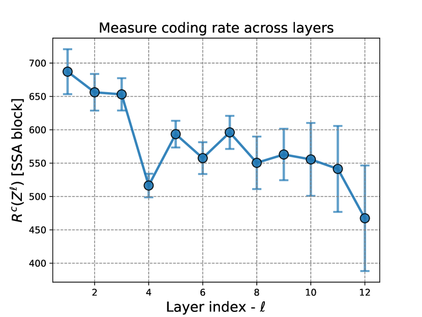
(a) Compression (Model: crate-Tiny).

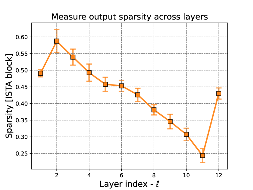
(b) Sparsity (Model: crate-Tiny).

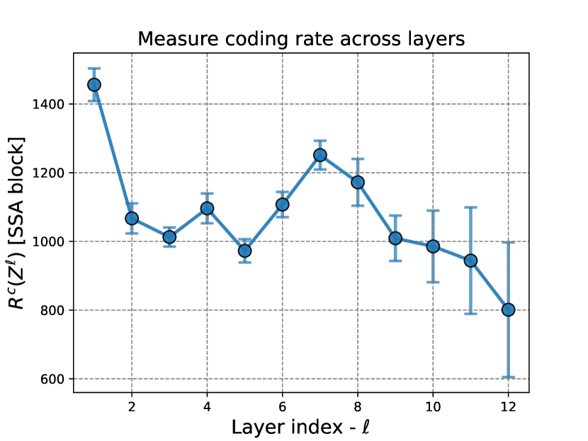
(c) Compression (Model: crate-Base).

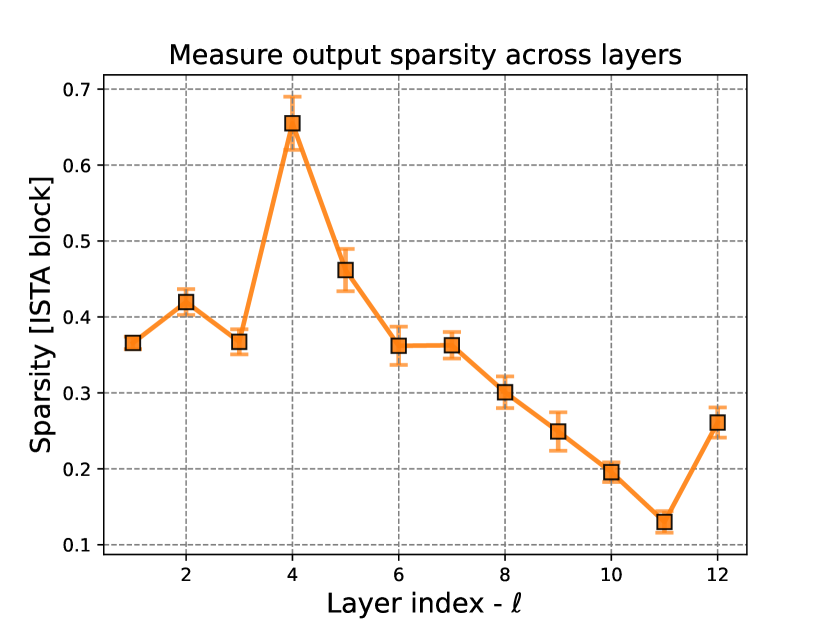
(d) Sparsity (Model: crate-Base).

(e) Compression (Model: crate-Large).

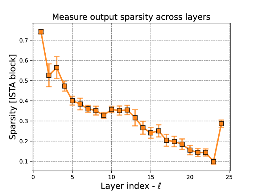
(f) Sparsity (Model: crate-Large).

Figure 20: Left: The compression term $R^{c}(\bm{Z}^{\ell+1/2})$ of the MSSA outputs at different layers. Right: the sparsity of the ISTA output block, $\lVert\bm{Z}^{\ell+1}\rVert_{0}/(d\cdot N)$, at different layers.

Visualizing layer-wise token representations.

In Figure 15, we visualize the token representations $\bm{Z}^{\ell}$ at different layers $\ell\in\{1,\dots,12\}$. We provide more results of the layer-wise token representation visualization on other samples in Figure 21, Figure 22, Figure 23, and Figure 24 (Model: crate-Base).

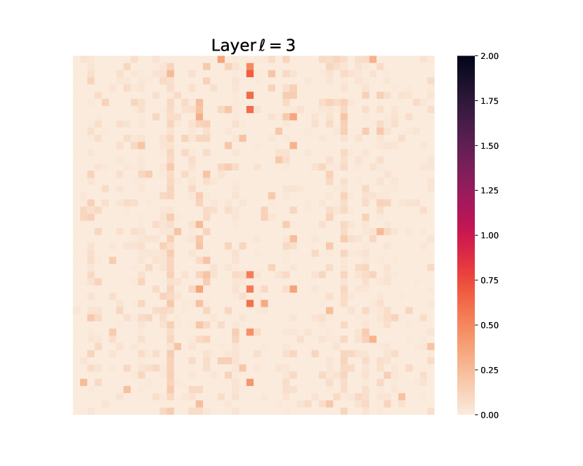
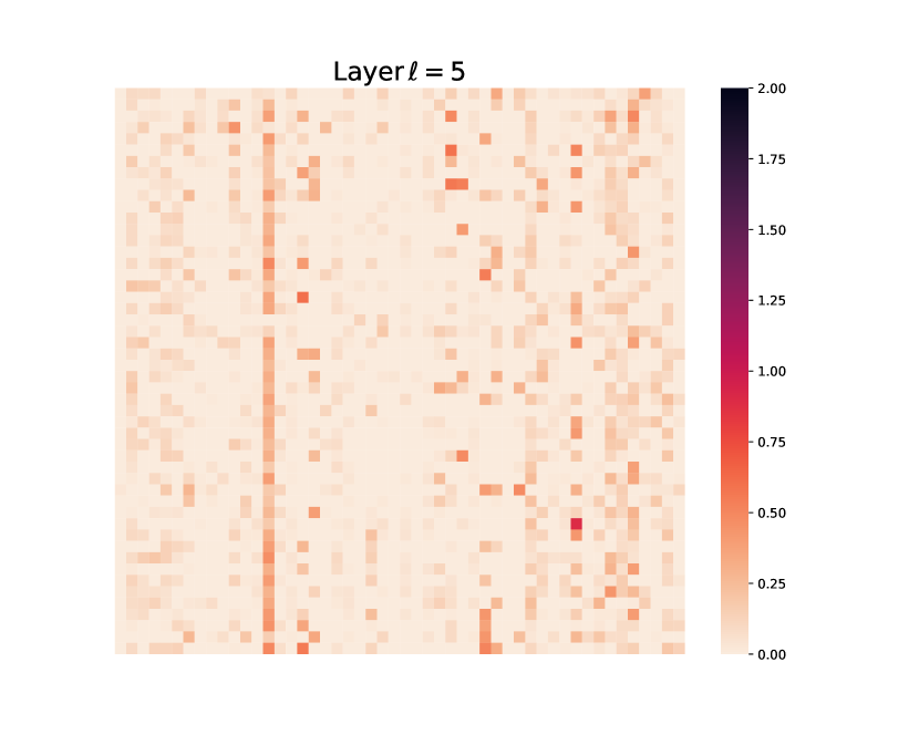
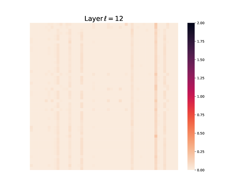
Figure 21: Visualizing layer-wise token $\bm{Z}^{\ell}$ representations at each layer $\ell$. To enhance the visual clarity, we randomly extract a 50$\times$50 sub-matrix from $\bm{Z}^{\ell}$ for display purposes. (Sample 1)

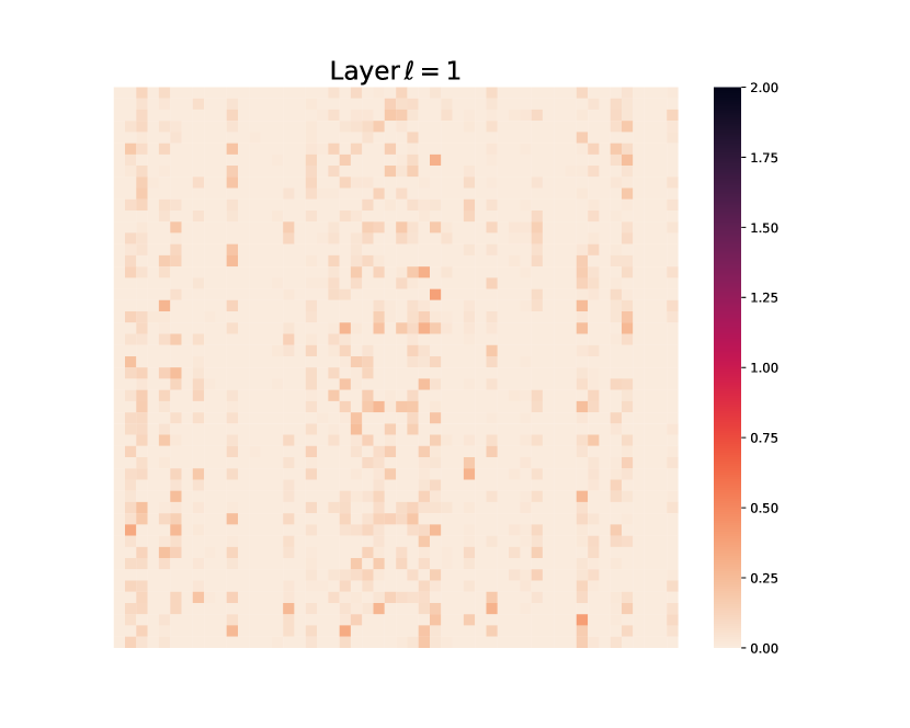
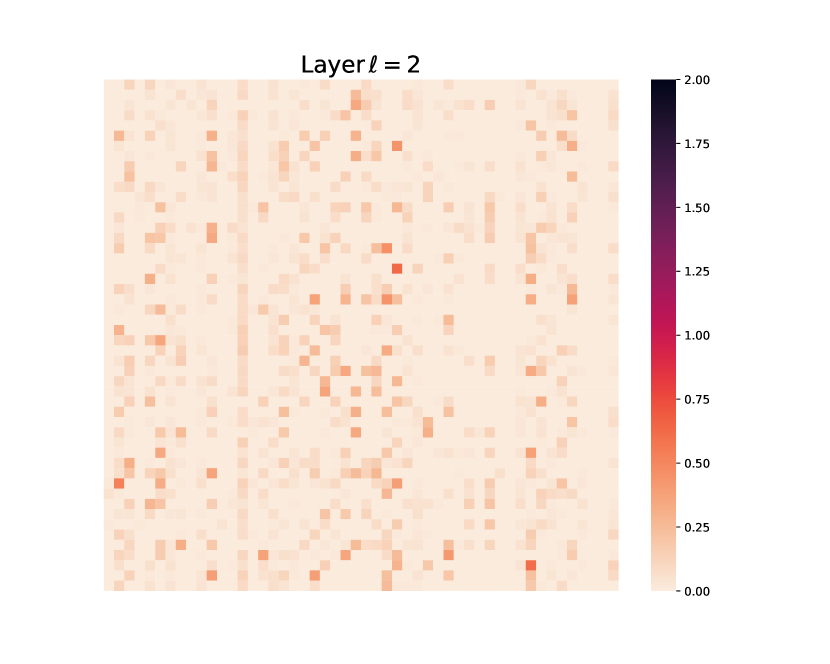
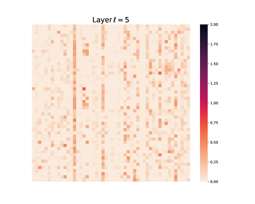
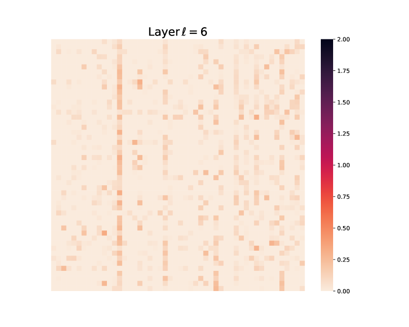
Figure 22: Visualizing layer-wise token $\bm{Z}^{\ell}$ representations at each layer $\ell$. To enhance the visual clarity, we randomly extract a 50$\times$50 sub-matrix from $\bm{Z}^{\ell}$ for display purposes. (Sample 2)

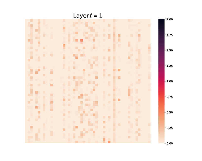
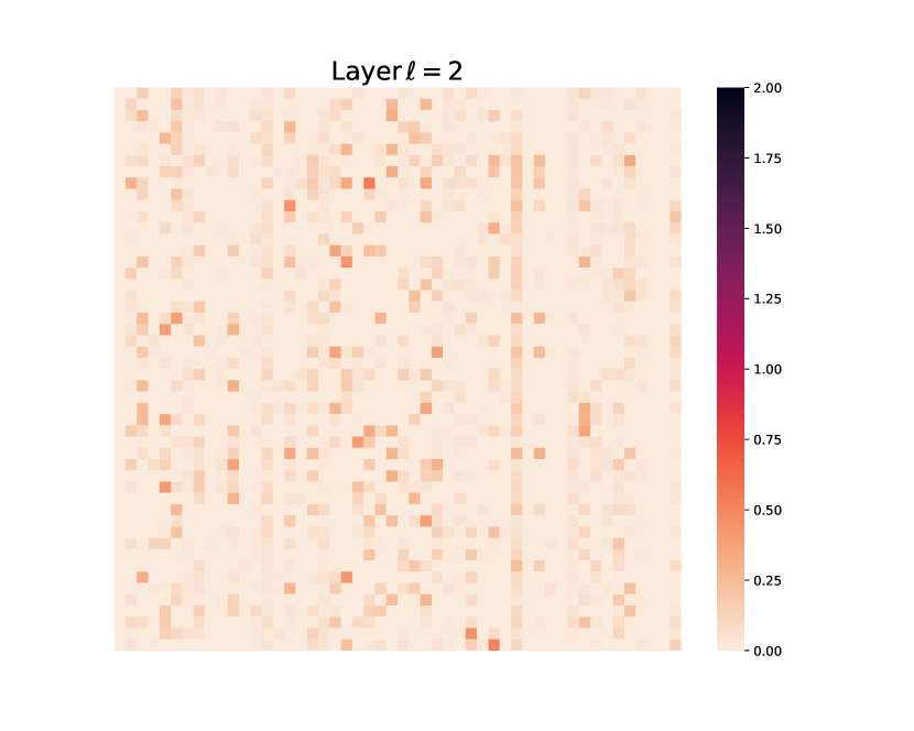
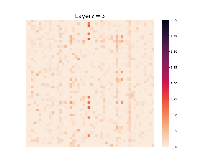
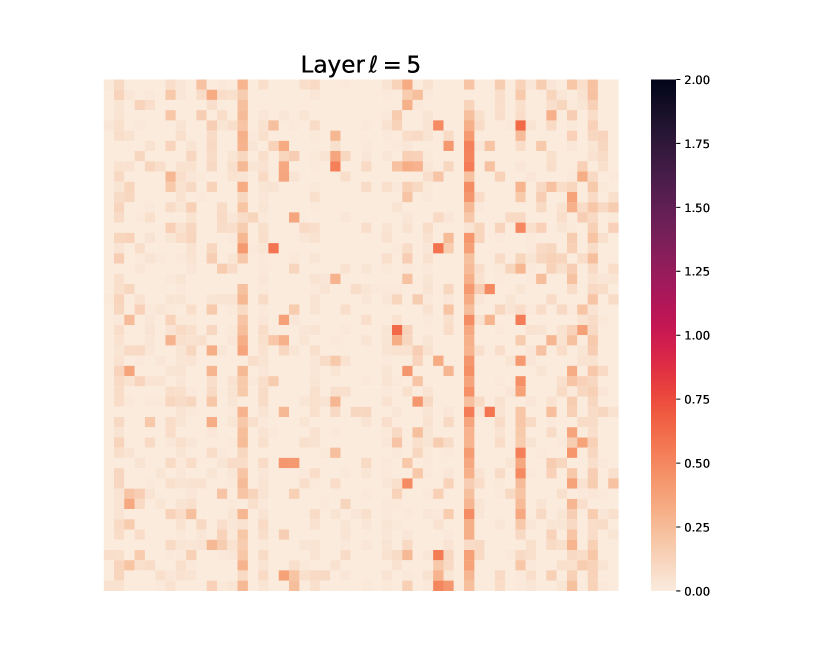
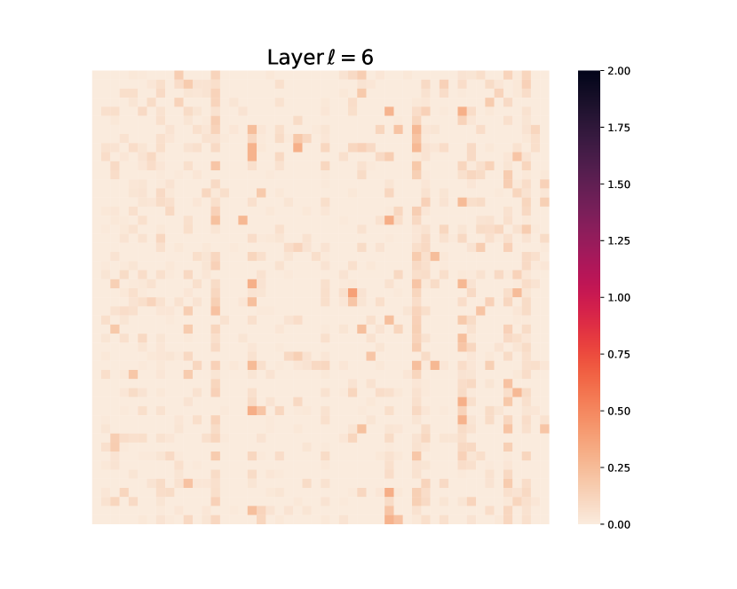
Figure 23: Visualizing layer-wise token $\bm{Z}^{\ell}$ representations at each layer $\ell$. To enhance the visual clarity, we randomly extract a 50$\times$50 sub-matrix from $\bm{Z}^{\ell}$ for display purposes. (Sample 3)

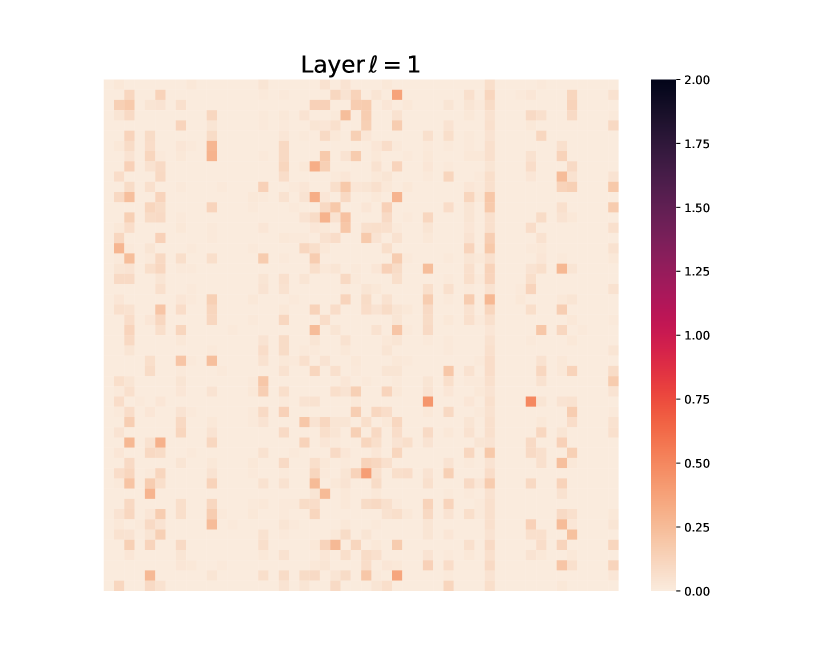
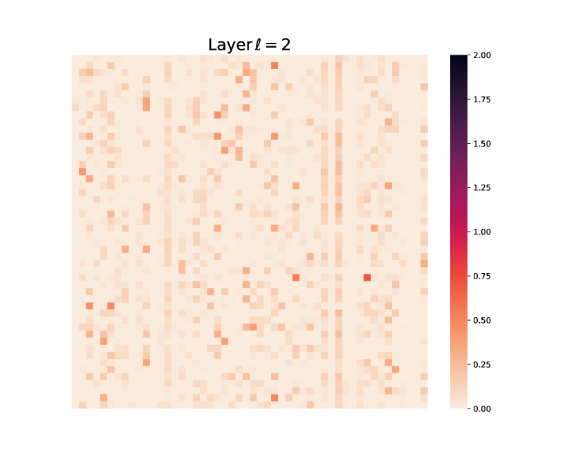
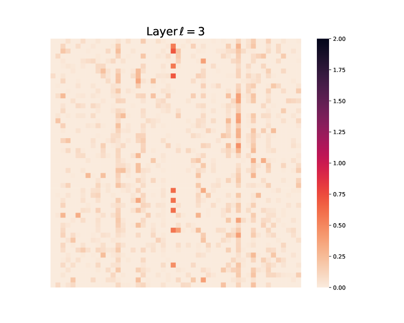
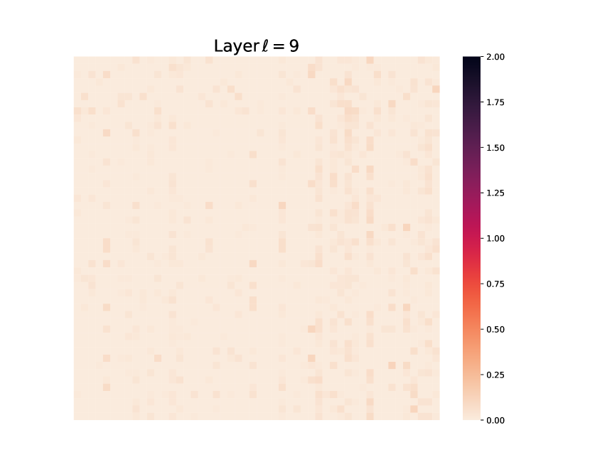
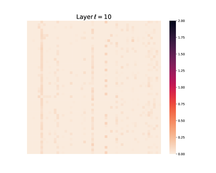
Figure 24: Visualizing layer-wise token $\bm{Z}^{\ell}$ representations at each layer $\ell$. To enhance the visual clarity, we randomly extract a 50$\times$50 sub-matrix from $\bm{Z}^{\ell}$ for display purposes. (Sample 4)

C.7 Details and Experimental Results of Attention Map Visualization

We recapitulate the method to visualize attention maps in Abnar and Zuidema (2020); Caron et al. (2021), at first specializing their use to instances of the crate model before generalizing to the ViT.

For the $k^{\mathrm{th}}$ head at the $\ell^{\mathrm{th}}$ layer of crate, we compute the self-attention matrix $\bm{A}_{k}^{\ell}\in\mathbb{R}^{n}$ defined as follows:

$$\bm{A}_{k}^{\ell}=\begin{bmatrix}A_{k,1}^{\ell}\\ \vdots\\ A_{k,N}^{\ell}\end{bmatrix}\in\mathbb{R}^{N},\quad\text{where}\quad A_{k,i}^{\ell}=\frac{\exp(\langle\bm{U}^{\ell*}_{k}\bm{z}^{\ell}_{i},\bm{U}^{\ell*}_{k}\bm{z}^{\ell}_{\texttt{[CLS]}}\rangle)}{\sum_{j=1}^{N}\exp(\langle\bm{U}^{\ell*}_{k}\bm{z}^{\ell}_{j},\bm{U}^{\ell*}_{k}\bm{z}^{\ell}_{\texttt{[CLS]}}\rangle)}.$$ (432)

We then reshape the attention matrix $\bm{A}_{k}^{\ell}$ into a ${\sqrt{n}\times\sqrt{n}}$ matrix and visualize the heatmap as shown in Figure 19. For example, the $i^{\mathrm{th}}$ row and the $j^{\mathrm{th}}$ column element of the heatmap in Figure 19 corresponds to the $m^{\mathrm{th}}$ component of $\bm{A}_{k}^{\ell}$ if $m=(i-1)\cdot\sqrt{n}+j$. In Figure 19, we select 4 attention heads of crate and visualize the attention matrix $\bm{A}_{k}^{\ell}$ for each image.

For the ViT, the entire methodology remains the same, except that the attention map is defined in the following reasonable way:

$$\bm{A}_{k}^{\ell}=\begin{bmatrix}A_{k,1}^{\ell}\\ \vdots\\ A_{k,N}^{\ell}\end{bmatrix}\in\mathbb{R}^{N},\quad\text{where}\quad A_{k,i}^{\ell}=\frac{\exp(\langle\bm{K}^{\ell*}_{k}\bm{z}^{\ell}_{i},\bm{Q}^{\ell*}_{k}\bm{z}^{\ell}_{\texttt{[CLS]}}\rangle)}{\sum_{j=1}^{N}\exp(\langle\bm{K}^{\ell*}_{k}\bm{z}^{\ell}_{j},\bm{Q}^{\ell*}_{k}\bm{z}^{\ell}_{\texttt{[CLS]}}\rangle)}.$$ (433)

where the “query” and “key” parameters of the standard transformer at head $k$ and layer $\ell$ are denoted $\bm{K}_{k}^{\ell}$ and $\bm{Q}_{k}^{\ell}$ respectively.

Details about MaskCut.

We apply the MaskCut pipeline (Algorithm 1) to generate segmentation masks and detection bounding box (discussed in Section 4.3.2). As described by Wang et al. (2023b), we iteratively apply Normalized Cuts (Shi and Malik, 2000) on the patch-wise affinity matrix $\bm{M}^{\ell}$, where $\bm{M}_{ij}^{\ell}=\sum_{k=1}^{K}\langle\bm{U}^{\ell*}_{k}\bm{z}_{i}^{\ell},\bm{U}^{\ell*}_{k}\bm{z}_{j}^{\ell}\rangle$. At each iterative step, we mask out the identified patch-wise entries on $\bm{M}^{\ell}$. To obtain more fine-grained segmentation masks, MaskCut employs Conditional Random Fields (CRF) (Krähenbühl and Koltun, 2011) to post-process the masks, which smooths the edges and filters out unreasonable masks. Correspondingly, the detection bounding box is defined by the rectangular region that tightly encloses a segmentation mask.

1

Hyperparameter: $S$, the number of objects to segment.

2

3Function MaskCut($\bm{M}$):

4       for $i\in\{1,\dots,S\}$ do

             mask $\leftarrow$ NCut($\bm{M}$) ;

              // mask is a boolean array

             $\bm{M}\leftarrow\bm{M}\odot\texttt{mask}$ ;

              // Equivalent to applying the mask to $\bm{M}$

5             masks[i] $\leftarrow$ mask;

6            

7       endfor

8      

9 return masks

Algorithm 1 MaskCut

Additional visualization of attention map.

We provide additional experiments on comparing the attention maps of crate and ViT in Figure 25.

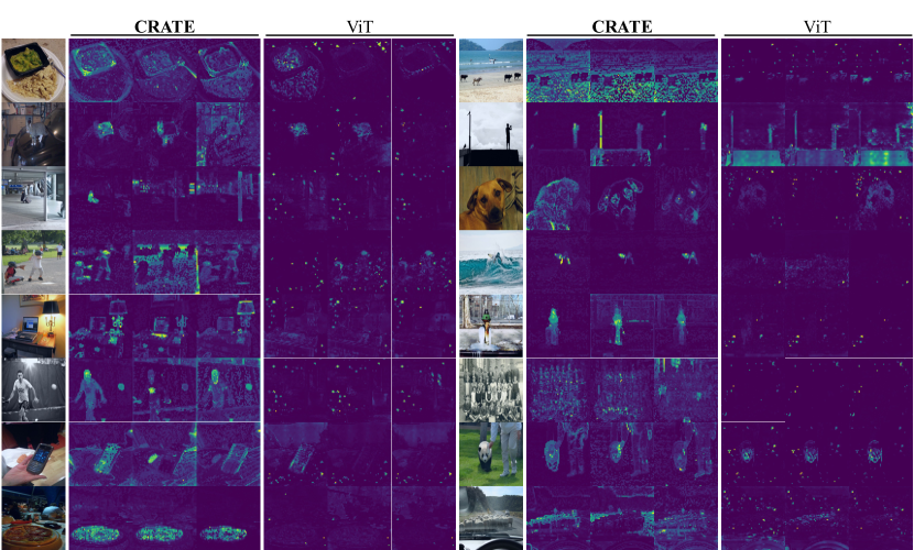
Figure 25: More attention maps of supervised crate and ViT on images from COCO val2017. We select the second-to-last layer attention maps to visualize for crate and the last layer for ViT.

Appendix D PyTorch code for CRATE

We provide PyTorch-style code for implementing our proposed network architecture crate, including the encoder architecture in Section 2 and the decoder architecture described in Section 3.

• In Section D.1, we provide the PyTorch-style pseudocode for the MSSA and ISTA blocks.

• In Section D.2, we provide the PyTorch-style pseudocode for an encoder layer $f^{\ell}$ of the crate transformer.

• In Section D.3, we provide the PyTorch style pseudocode for a decoder layer $g^{\ell}$ of the crate transformer.

• In Section D.4, as an example of all the top-level architectures we implement for experiments in Section 4, we implement the crate image classifier.

D.1 PyTorch-Like Pseudocode for MSSA and ISTA Blocks

⬇

class MSSA:

# initialization

def __init__(self, dim, heads = 8, dim_head = 64, dropout = 0.):

inner_dim = dim_head * heads

project_out = not (heads == 1 and dim_head == dim)

self.heads = heads

self.scale = dim_head ** -0.5

self.attend = Softmax(dim = -1)

self.dropout = Dropout(dropout)

self.qkv = Linear(dim, inner_dim, bias=False)

self.to_out = Sequential(Linear(inner_dim, dim), Dropout(dropout)) if project_out else nn.Identity()

\par# forward pass

def forward(self, x):

w = rearrange(self.qkv(x), ’b n (h d) -> b h n d’, h = self.heads)

dots = matmul(w, w.transpose(-1, -2)) * self.scale

attn = self.attend(dots)

attn = self.dropout(attn)

out = matmul(attn, w)

out = rearrange(out, ’b h n d -> b n (h d)’)

return self.to_out(out)

Algorithm 2 PyTorch-style pseudocode for MSSA block in transformer.

⬇

class ISTA:

# initialization

def __init__(self, dim, dropout = 0., step_size=0.1, lambd=0.1):

super().__init__()

self.weight = nn.Parameter(torch.Tensor(dim, dim))

with torch.no_grad():

init.kaiming_uniform_(self.weight)

self.step_size = step_size

self.lambd = lambd

\par# forward pass

def forward(self, x):

x1 = F.linear(x, self.weight, bias=None)

grad_update = self.step_size * F.linear(x1 - x, self.weight.t(), bias=None)

output = F.relu(x - grad_update - self.step_size * self.lambd)

return output

Algorithm 3 PyTorch-style pseudocode for ISTA block in transformer.

D.2 PyTorch-Like Pseudocode for CRATE Encoder

⬇

class CRATEEncoder(Module):

# initialization

def __init__(self, dim, depth, heads, dim_head, dropout = 0.):

self.layers = []

self.depth = depth

for _ in range(depth):

self.layers.extend([LayerNorm(dim), MSSA(dim, heads, dim_head, dropout)])

self.layers.extend([LayerNorm(dim), ISTA(dim, dropout)])

\par# forward pass

def forward(self, x):

for ln1, attn, ln2, ff in self.layers:

x_ = attn(ln1(x)) + ln1(x)

x = ff(ln2(x_))

return x

Algorithm 4 PyTorch-style pseudocode for crate encoder.

D.3 PyTorch-Like Pseudocode for CRATE Decoder

⬇

class CRATEDecoder(Module):

# initialization

def __init__(self, dim, depth, heads, dim_head, dropout = 0.):

self.layers = []

self.depth = depth

for _ in range(depth):

self.layers.extend([LayerNorm(dim), Linear(dim)])

self.layers.extend([LayerNorm(dim), MSSA(dim, heads, dim_head, dropout)])

\par# forward pass

def forward(self, x):

for ln1, lin, ln2, attn in self.layers:

x_ = lin(ln1(x))

x = ln2(x_) - attn(ln2(x_))

return x

Algorithm 5 PyTorch-style pseudocode for crate decoder.

D.4 PyTorch-Like Pseudocode for CRATE Image Classifier

⬇

class CRATEClassifier(Module):

# initialization

def init(self, image_size, patch_size, num_classes, dim, depth, heads, channels = 3, dim_head = 64, dropout = 0., emb_dropout = 0.):

# define patch, image dimensions and number of patches

image_height, image_width = pair(image_size)

patch_height, patch_width = pair(patch_size)

num_patches = (image_height // patch_height) * (image_width // patch_width)

patch_dim = channels * patch_height * patch_width

\par# define patch embedding, positional embedding, dropout, and transformer

self.to_patch_embedding = Sequential(Rearrange, LayerNorm(patch_dim), Linear(patch_dim, dim), LayerNorm(dim))

self.pos_embedding = Parameter(random(1, num_patches + 1, dim))

self.cls_token = Parameter(random(1, 1, dim))

self.dropout = Dropout(emb_dropout)

self.transformer = CRATEEncoder(dim, depth, heads, dim_head, dropout)

\par# define pooling, latent layer, and MLP head

self.pool = pool

self.to_latent = Identity()

self.mlp_head = Sequential(LayerNorm(dim), Linear(dim, num_classes))

\par# forward pass

def forward(self, img):

x = self.to_patch_embedding(img)

b, n, _ = shape(x)

cls_tokens = repeat(self.cls_token, ’1 1 d -> b 1 d’, b = b)

x = concatenate((cls_tokens, x), dim=1)

x += self.pos_embedding[:, :(n + 1)]

x = self.dropout(x)

x = self.transformer(x)

x = mean(x, dim = 1) if self.pool == ’mean’ else x[:, 0]

x = self.to_latent(x)

return self.mlp_head(x)

Algorithm 6 PyTorch-style pseudocode for crate image classifier.

References

- Abnar and Zuidema (2020) Samira Abnar and Willem H. Zuidema. Quantifying Attention Flow in Transformers. In Dan Jurafsky, Joyce Chai, Natalie Schluter, and Joel R. Tetreault, editors, Proceedings of the 58th Annual Meeting of the Association for Computational Linguistics, ACL 2020, Online, July 5-10, 2020, pages 4190–4197. Association for Computational Linguistics, 2020. doi: 10.18653/V1/2020.ACL-MAIN.385. URL https://doi.org/10.18653/v1/2020.acl-main.385.
- Aharon et al. (2006) Michal Aharon, Michael Elad, and Alfred M. Bruckstein. K-SVD: An algorithm for designing overcomplete dictionaries for sparse representation. IEEE Trans. Signal Process., 54(11):4311–4322, 2006. doi: 10.1109/TSP.2006.881199. URL https://doi.org/10.1109/TSP.2006.881199.
- Arnab et al. (2021) Anurag Arnab, Mostafa Dehghani, Georg Heigold, Chen Sun, Mario Lucic, and Cordelia Schmid. ViViT: A Video Vision Transformer. In 2021 IEEE/CVF International Conference on Computer Vision, ICCV 2021, Montreal, QC, Canada, October 10-17, 2021, pages 6816–6826. IEEE, 2021. doi: 10.1109/ICCV48922.2021.00676. URL https://doi.org/10.1109/ICCV48922.2021.00676.
- Bakry et al. (2016) Dominique Bakry, Ivan Gentil, and Michel Ledoux. Analysis and Geometry of Markov Diffusion Operators. Springer International Publishing, August 2016. ISBN 9783319343235. URL https://play.google.com/store/books/details?id=tQICvgAACAAJ.
- Bardes et al. (2022) Adrien Bardes, Jean Ponce, and Yann LeCun. VICReg: Variance-Invariance-covariance Regularization for Self-supervised Learning. In International Conference on Learning Representations, 2022. URL https://openreview.net/forum?id=xm6YD62D1Ub.
- Beck and Teboulle (2009) Amir Beck and Marc Teboulle. A Fast Iterative Shrinkage-thresholding Algorithm for Linear Inverse Problems. SIAM J. Imaging Sci., 2(1):183–202, 2009. doi: 10.1137/080716542. URL https://doi.org/10.1137/080716542.
- Betker et al. (2023) James Betker, Gabriel Goh, Li Jing, et al. Improving Image Generation with Better Captions. 2023.
- Bommasani et al. (2021) Rishi Bommasani, Drew A. Hudson, Ehsan Adeli, Russ B. Altman, Simran Arora, Sydney von Arx, Michael S. Bernstein, Jeannette Bohg, Antoine Bosselut, Emma Brunskill, Erik Brynjolfsson, Shyamal Buch, Dallas Card, Rodrigo Castellon, Niladri S. Chatterji, Annie S. Chen, Kathleen Creel, Jared Quincy Davis, Dorottya Demszky, Chris Donahue, Moussa Doumbouya, Esin Durmus, Stefano Ermon, John Etchemendy, Kawin Ethayarajh, Li Fei-Fei, Chelsea Finn, Trevor Gale, Lauren Gillespie, Karan Goel, Noah D. Goodman, Shelby Grossman, Neel Guha, Tatsunori Hashimoto, Peter Henderson, John Hewitt, Daniel E. Ho, Jenny Hong, Kyle Hsu, Jing Huang, Thomas Icard, Saahil Jain, Dan Jurafsky, Pratyusha Kalluri, Siddharth Karamcheti, Geoff Keeling, Fereshte Khani, Omar Khattab, Pang Wei Koh, Mark S. Krass, Ranjay Krishna, Rohith Kuditipudi, and et al. On the Opportunities and Risks of Foundation Models. CoRR, abs/2108.07258, 2021. URL https://arxiv.org/abs/2108.07258.
- Brown et al. (2020) Tom B. Brown, Benjamin Mann, Nick Ryder, Melanie Subbiah, Jared Kaplan, Prafulla Dhariwal, Arvind Neelakantan, Pranav Shyam, Girish Sastry, Amanda Askell, Sandhini Agarwal, Ariel Herbert-Voss, Gretchen Krueger, Tom Henighan, Rewon Child, Aditya Ramesh, Daniel M. Ziegler, Jeffrey Wu, Clemens Winter, Christopher Hesse, Mark Chen, Eric Sigler, Mateusz Litwin, Scott Gray, Benjamin Chess, Jack Clark, Christopher Berner, Sam McCandlish, Alec Radford, Ilya Sutskever, and Dario Amodei. Language Models are Few-shot Learners. In Hugo Larochelle, Marc’Aurelio Ranzato, Raia Hadsell, Maria-Florina Balcan, and Hsuan-Tien Lin, editors, Advances in Neural Information Processing Systems 33: Annual Conference on Neural Information Processing Systems 2020, NeurIPS 2020, December 6-12, 2020, virtual, 2020. URL https://proceedings.neurips.cc/paper/2020/hash/1457c0d6bfcb4967418bfb8ac142f64a-Abstract.html.
- Bruna and Mallat (2013) Joan Bruna and Stéphane Mallat. Invariant Scattering Convolution Networks. IEEE Trans. Pattern Anal. Mach. Intell., 35(8):1872–1886, 2013. doi: 10.1109/TPAMI.2012.230. URL https://doi.org/10.1109/TPAMI.2012.230.
- Carion et al. (2020) Nicolas Carion, Francisco Massa, Gabriel Synnaeve, Nicolas Usunier, Alexander Kirillov, and Sergey Zagoruyko. End-to-end Object Detection with Transformers. In Andrea Vedaldi, Horst Bischof, Thomas Brox, and Jan-Michael Frahm, editors, Computer Vision - ECCV 2020 - 16th European Conference, Glasgow, UK, August 23-28, 2020, Proceedings, Part I, volume 12346 of Lecture Notes in Computer Science, pages 213–229. Springer, 2020. doi: 10.1007/978-3-030-58452-8“˙13. URL https://doi.org/10.1007/978-3-030-58452-8_13.
- Caron et al. (2020) Mathilde Caron, Ishan Misra, Julien Mairal, Priya Goyal, Piotr Bojanowski, and Armand Joulin. Unsupervised Learning of Visual Features by Contrasting Cluster Assignments. In Hugo Larochelle, Marc’Aurelio Ranzato, Raia Hadsell, Maria-Florina Balcan, and Hsuan-Tien Lin, editors, Advances in Neural Information Processing Systems 33: Annual Conference on Neural Information Processing Systems 2020, NeurIPS 2020, December 6-12, 2020, virtual, 2020. URL https://proceedings.neurips.cc/paper/2020/hash/70feb62b69f16e0238f741fab228fec2-Abstract.html.
- Caron et al. (2021) Mathilde Caron, Hugo Touvron, Ishan Misra, Hervé Jégou, Julien Mairal, Piotr Bojanowski, and Armand Joulin. Emerging Properties in Self-supervised Vision Transformers. In 2021 IEEE/CVF International Conference on Computer Vision, ICCV 2021, Montreal, QC, Canada, October 10-17, 2021, pages 9630–9640. IEEE, 2021. doi: 10.1109/ICCV48922.2021.00951. URL https://doi.org/10.1109/ICCV48922.2021.00951.
- Chan et al. (2022) Kwan Ho Ryan Chan, Yaodong Yu, Chong You, Haozhi Qi, John Wright, and Yi Ma. ReduNet: A White-box Deep Network from the Principle of Maximizing Rate Reduction. Journal of Machine Learning Research, 23(114):1–103, 2022. URL http://jmlr.org/papers/v23/21-0631.html.
- Chen et al. (2023a) Hongrui Chen, Holden Lee, and Jianfeng Lu. Improved Analysis of Score-based Generative Modeling: User-friendly Bounds under Minimal Smoothness Assumptions. In Andreas Krause, Emma Brunskill, Kyunghyun Cho, Barbara Engelhardt, Sivan Sabato, and Jonathan Scarlett, editors, International Conference on Machine Learning, ICML 2023, 23-29 July 2023, Honolulu, Hawaii, USA, volume 202 of Proceedings of Machine Learning Research, pages 4735–4763. PMLR, 2023a. URL https://proceedings.mlr.press/v202/chen23q.html.
- Chen et al. (2020) Ting Chen, Simon Kornblith, Mohammad Norouzi, and Geoffrey E. Hinton. A Simple Framework for Contrastive Learning of Visual Representations. In Proceedings of the 37th International Conference on Machine Learning, ICML 2020, 13-18 July 2020, Virtual Event, volume 119 of Proceedings of Machine Learning Research, pages 1597–1607. PMLR, 2020. URL http://proceedings.mlr.press/v119/chen20j.html.
- Chen et al. (2023b) Xiangning Chen, Chen Liang, Da Huang, Esteban Real, Kaiyuan Wang, Yao Liu, Hieu Pham, Xuanyi Dong, Thang Luong, Cho-Jui Hsieh, Yifeng Lu, and Quoc V. Le. Symbolic Discovery of Optimization Algorithms. CoRR, abs/2302.06675, 2023b. doi: 10.48550/ARXIV.2302.06675. URL https://doi.org/10.48550/arXiv.2302.06675.
- Chen et al. (2018) Yubei Chen, Dylan M. Paiton, and Bruno A. Olshausen. The Sparse Manifold Transform. In Samy Bengio, Hanna M. Wallach, Hugo Larochelle, Kristen Grauman, Nicolò Cesa-Bianchi, and Roman Garnett, editors, Advances in Neural Information Processing Systems 31: Annual Conference on Neural Information Processing Systems 2018, NeurIPS 2018, December 3-8, 2018, Montréal, Canada, pages 10534–10545, 2018. URL https://proceedings.neurips.cc/paper/2018/hash/8e19a39c36b8e5e3afd2a3b2692aea96-Abstract.html.
- Cover (1999) Thomas M Cover. Elements of information theory. John Wiley & Sons, 1999.
- Dai et al. (2022) Xili Dai, Shengbang Tong, Mingyang Li, Ziyang Wu, Michael Psenka, Kwan Ho Ryan Chan, Pengyuan Zhai, Yaodong Yu, Xiaojun Yuan, Heung-Yeung Shum, and Yi Ma. CTRL: Closed-loop Transcription to an LDR via Minimaxing Rate Reduction. Entropy, 24(4):456, 2022. doi: 10.3390/E24040456. URL https://doi.org/10.3390/e24040456.
- Dai et al. (2023) Xili Dai, Ke Chen, Shengbang Tong, Jingyuan Zhang, Xingjian Gao, Mingyang Li, Druv Pai, Yuexiang Zhai, Xiaojun Yuan, Heung-Yeung Shum, Lionel M. Ni, and Yi Ma. Closed-loop Transcription via Convolutional Sparse Coding. CoRR, abs/2302.09347, 2023. doi: 10.48550/ARXIV.2302.09347. URL https://doi.org/10.48550/arXiv.2302.09347.
- Dehghani et al. (2023) Mostafa Dehghani, Josip Djolonga, Basil Mustafa, Piotr Padlewski, Jonathan Heek, Justin Gilmer, Andreas Peter Steiner, Mathilde Caron, Robert Geirhos, Ibrahim Alabdulmohsin, Rodolphe Jenatton, Lucas Beyer, Michael Tschannen, Anurag Arnab, Xiao Wang, Carlos Riquelme Ruiz, Matthias Minderer, Joan Puigcerver, Utku Evci, Manoj Kumar, Sjoerd van Steenkiste, Gamaleldin Fathy Elsayed, Aravindh Mahendran, Fisher Yu, Avital Oliver, Fantine Huot, Jasmijn Bastings, Mark Collier, Alexey A. Gritsenko, Vighnesh Birodkar, Cristina Nader Vasconcelos, Yi Tay, Thomas Mensink, Alexander Kolesnikov, Filip Pavetic, Dustin Tran, Thomas Kipf, Mario Lucic, Xiaohua Zhai, Daniel Keysers, Jeremiah J. Harmsen, and Neil Houlsby. Scaling Vision Transformers to 22 Billion Parameters. In Andreas Krause, Emma Brunskill, Kyunghyun Cho, Barbara Engelhardt, Sivan Sabato, and Jonathan Scarlett, editors, International Conference on Machine Learning, ICML 2023, 23-29 July 2023, Honolulu, Hawaii, USA, volume 202 of Proceedings of Machine Learning Research, pages 7480–7512. PMLR, 2023. URL https://proceedings.mlr.press/v202/dehghani23a.html.
- Deng et al. (2009) Jia Deng, Wei Dong, Richard Socher, Li-Jia Li, Kai Li, and Li Fei-Fei. ImageNet: A large-scale hierarchical image database. In 2009 IEEE Computer Society Conference on Computer Vision and Pattern Recognition (CVPR 2009), 20-25 June 2009, Miami, Florida, USA, pages 248–255. IEEE Computer Society, 2009. doi: 10.1109/CVPR.2009.5206848. URL https://doi.org/10.1109/CVPR.2009.5206848.
- Devlin et al. (2019) Jacob Devlin, Ming-Wei Chang, Kenton Lee, and Kristina Toutanova. BERT: Pre-training of Deep Bidirectional Transformers for Language Understanding. In Jill Burstein, Christy Doran, and Thamar Solorio, editors, Proceedings of the 2019 Conference of the North American Chapter of the Association for Computational Linguistics: Human Language Technologies, NAACL-HLT 2019, Minneapolis, MN, USA, June 2-7, 2019, Volume 1 (Long and Short Papers), pages 4171–4186. Association for Computational Linguistics, 2019. doi: 10.18653/V1/N19-1423. URL https://doi.org/10.18653/v1/n19-1423.
- Donoho and Grimes (2005) David L. Donoho and Carrie Grimes. Image Manifolds which are Isometric to Euclidean Space. J. Math. Imaging Vis., 23(1):5–24, 2005. doi: 10.1007/S10851-005-4965-4. URL https://doi.org/10.1007/s10851-005-4965-4.
- Dosovitskiy et al. (2021) Alexey Dosovitskiy, Lucas Beyer, Alexander Kolesnikov, Dirk Weissenborn, Xiaohua Zhai, Thomas Unterthiner, Mostafa Dehghani, Matthias Minderer, Georg Heigold, Sylvain Gelly, Jakob Uszkoreit, and Neil Houlsby. An Image is Worth 16x16 Words: Transformers for Image Recognition at Scale. In 9th International Conference on Learning Representations, ICLR 2021, Virtual Event, Austria, May 3-7, 2021. OpenReview.net, 2021. URL https://openreview.net/forum?id=YicbFdNTTy.
- Efron (2011a) Bradley Efron. Tweedie’s Formula and Selection Bias. Journal of the American Statistical Association, 106(496):1602–1614, 2011a. ISSN 0162-1459. doi: 10.1198/jasa.2011.tm11181. URL http://dx.doi.org/10.1198/jasa.2011.tm11181.
- Efron (2011b) Bradley Efron. Tweedie’s formula and selection bias. Journal of the American Statistical Association, 106(496):1602–1614, 2011b.
- Elad (2010) Michael Elad. Sparse and Redundant Representations - From Theory to Applications in Signal and Image Processing. Springer, 2010. ISBN 978-1-4419-7010-7. doi: 10.1007/978-1-4419-7011-4. URL https://doi.org/10.1007/978-1-4419-7011-4.
- Elad et al. (2010) Michael Elad, Mário A. T. Figueiredo, and Yi Ma. On the Role of Sparse and Redundant Representations in Image Processing. Proc. IEEE, 98(6):972–982, 2010. doi: 10.1109/JPROC.2009.2037655. URL https://doi.org/10.1109/JPROC.2009.2037655.
- Fang et al. (2021) Cong Fang, Hangfeng He, Qi Long, and Weijie J Su. Exploring deep neural networks via layer-peeled model: Minority collapse in imbalanced training. Proceedings of the National Academy of Sciences, 118(43):e2103091118, 2021.
- Felzenszwalb and Huttenlocher (2005) Pedro F Felzenszwalb and Daniel P Huttenlocher. Pictorial Structures for Object Recognition. International journal of computer vision, 61(1):55–79, January 2005. ISSN 0920-5691, 1573-1405. doi: 10.1023/B:VISI.0000042934.15159.49. URL https://doi.org/10.1023/B:VISI.0000042934.15159.49.
- Felzenszwalb et al. (2008) Pedro F. Felzenszwalb, David A. McAllester, and Deva Ramanan. A discriminatively trained, multiscale, deformable part model. In 2008 IEEE Computer Society Conference on Computer Vision and Pattern Recognition (CVPR 2008), 24-26 June 2008, Anchorage, Alaska, USA. IEEE Computer Society, 2008. doi: 10.1109/CVPR.2008.4587597. URL https://doi.org/10.1109/CVPR.2008.4587597.
- Gao and Pavel (2017) Bolin Gao and Lacra Pavel. On the Properties of the Softmax Function with Application in Game Theory and Reinforcement Learning. CoRR, abs/1704.00805, 2017. URL http://arxiv.org/abs/1704.00805.
- Ge et al. (2018) Rong Ge, Holden Lee, and Andrej Risteski. Simulated Tempering Langevin Monte Carlo II: An Improved Proof using Soft Markov Chain Decomposition. CoRR, abs/1812.00793, 2018. URL http://arxiv.org/abs/1812.00793.
- Gokaslan and Cohen (2019) Aaron Gokaslan and Vanya Cohen. OpenWebText Corpus, 2019.
- Gong et al. (2023) Yuan Gong, Andrew Rouditchenko, Alexander H. Liu, David Harwath, Leonid Karlinsky, Hilde Kuehne, and James R. Glass. Contrastive Audio-visual Masked Autoencoder. In The Eleventh International Conference on Learning Representations, ICLR 2023, Kigali, Rwanda, May 1-5, 2023. OpenReview.net, 2023. URL https://openreview.net/pdf?id=QPtMRyk5rb.
- Google (2021) Google. huggingface BERT releases. https://huggingface.co/google/bert_uncased_L-8_H-512_A-8/tree/main, 2021.
- Gregor and LeCun (2010) Karol Gregor and Yann LeCun. Learning Fast Approximations of Sparse Coding. In Johannes Fürnkranz and Thorsten Joachims, editors, Proceedings of the 27th International Conference on Machine Learning (ICML-10), June 21-24, 2010, Haifa, Israel, pages 399–406. Omnipress, 2010. URL https://icml.cc/Conferences/2010/papers/449.pdf.
- Gribonval et al. (2015) Rémi Gribonval, Rodolphe Jenatton, and Francis R. Bach. Sparse and Spurious: Dictionary Learning With Noise and Outliers. IEEE Trans. Inf. Theory, 61(11):6298–6319, 2015. doi: 10.1109/TIT.2015.2472522. URL https://doi.org/10.1109/TIT.2015.2472522.
- Guth et al. (2022) Florentin Guth, John Zarka, and Stéphane Mallat. Phase Collapse in Neural Networks. In The Tenth International Conference on Learning Representations, ICLR 2022, Virtual Event, April 25-29, 2022. OpenReview.net, 2022. URL https://openreview.net/forum?id=iPHLcmtietq.
- Haussmann and Pardoux (1986) U G Haussmann and E Pardoux. Time Reversal of Diffusions. The Annals of Probability, 14(4):1188–1205, October 1986. ISSN 0091-1798, 2168-894X. doi: 10.1214/aop/1176992362. URL https://projecteuclid.org/journals/annals-of-probability/volume-14/issue-4/Time-Reversal-of-Diffusions/10.1214/aop/1176992362.full.
- He and Su (2022a) Hangfeng He and Weijie J. Su. A Law of Data Separation in Deep Learning. CoRR, abs/2210.17020, 2022a. doi: 10.48550/ARXIV.2210.17020. URL https://doi.org/10.48550/arXiv.2210.17020.
- He and Su (2022b) Hangfeng He and Weijie J. Su. A Law of Data Separation in Deep Learning. CoRR, abs/2210.17020, 2022b. doi: 10.48550/ARXIV.2210.17020. URL https://doi.org/10.48550/arXiv.2210.17020.
- He et al. (2016) Kaiming He, Xiangyu Zhang, Shaoqing Ren, and Jian Sun. Deep Residual Learning for Image Recognition. In 2016 IEEE Conference on Computer Vision and Pattern Recognition, CVPR 2016, Las Vegas, NV, USA, June 27-30, 2016, pages 770–778. IEEE Computer Society, 2016. doi: 10.1109/CVPR.2016.90. URL https://doi.org/10.1109/CVPR.2016.90.
- He et al. (2020) Kaiming He, Georgia Gkioxari, Piotr Dollár, and Ross B. Girshick. Mask R-CNN. IEEE Trans. Pattern Anal. Mach. Intell., 42(2):386–397, 2020. doi: 10.1109/TPAMI.2018.2844175. URL https://doi.org/10.1109/TPAMI.2018.2844175.
- He et al. (2021) Kaiming He, Xinlei Chen, Saining Xie, Yanghao Li, Piotr Dollár, and Ross B. Girshick. Masked Autoencoders Are Scalable Vision Learners. CoRR, abs/2111.06377, 2021. URL https://arxiv.org/abs/2111.06377.
- He et al. (2022) Kaiming He, Xinlei Chen, Saining Xie, Yanghao Li, Piotr Dollár, and Ross B. Girshick. Masked Autoencoders Are Scalable Vision Learners. In IEEE/CVF Conference on Computer Vision and Pattern Recognition, CVPR 2022, New Orleans, LA, USA, June 18-24, 2022, pages 15979–15988. IEEE, 2022. doi: 10.1109/CVPR52688.2022.01553. URL https://doi.org/10.1109/CVPR52688.2022.01553.
- Hinton (2021) Geoffrey Hinton. How to represent part-whole hierarchies in a neural network, 2021.
- Hinton (2022) Geoffrey Hinton. The Forward-forward Algorithm: Some Preliminary Investigations, 2022.
- Hinton and Zemel (1993) Geoffrey E Hinton and Richard Zemel. Autoencoders, Minimum Description Length and Helmholtz Free Energy. In J. Cowan, G. Tesauro, and J. Alspector, editors, Advances in Neural Information Processing Systems, volume 6. Morgan-Kaufmann, 1993. URL https://proceedings.neurips.cc/paper_files/paper/1993/file/9e3cfc48eccf81a0d57663e129aef3cb-Paper.pdf.
- Hinton et al. (2011) Geoffrey E. Hinton, Alex Krizhevsky, and Sida D. Wang. Transforming Auto-encoders. In Timo Honkela, Wlodzislaw Duch, Mark A. Girolami, and Samuel Kaski, editors, Artificial Neural Networks and Machine Learning - ICANN 2011 - 21st International Conference on Artificial Neural Networks, Espoo, Finland, June 14-17, 2011, Proceedings, Part I, volume 6791 of Lecture Notes in Computer Science, pages 44–51. Springer, 2011. doi: 10.1007/978-3-642-21735-7“˙6. URL https://doi.org/10.1007/978-3-642-21735-7_6.
- Hinton et al. (2015) Geoffrey E. Hinton, Oriol Vinyals, and Jeffrey Dean. Distilling the Knowledge in a Neural Network. CoRR, abs/1503.02531, 2015. URL http://arxiv.org/abs/1503.02531.
- Ho et al. (2020) Jonathan Ho, Ajay Jain, and Pieter Abbeel. Denoising Diffusion Probabilistic Models. In Hugo Larochelle, Marc’Aurelio Ranzato, Raia Hadsell, Maria-Florina Balcan, and Hsuan-Tien Lin, editors, Advances in Neural Information Processing Systems 33: Annual Conference on Neural Information Processing Systems 2020, NeurIPS 2020, December 6-12, 2020, virtual, 2020. URL https://proceedings.neurips.cc/paper/2020/hash/4c5bcfec8584af0d967f1ab10179ca4b-Abstract.html.
- Hoover et al. (2023) Benjamin Hoover, Yuchen Liang, Bao Pham, Rameswar Panda, Hendrik Strobelt, Duen Horng Chau, Mohammed J. Zaki, and Dmitry Krotov. Energy Transformer. CoRR, abs/2302.07253, 2023. doi: 10.48550/ARXIV.2302.07253. URL https://doi.org/10.48550/arXiv.2302.07253.
- Huggingface (2020) Huggingface. huggingface text classification examples. https://github.com/huggingface/transformers/tree/main/examples/pytorch/text-classification, 2020.
- Huggingface (2023) Huggingface. huggingface CoLA GitHub Issue. https://github.com/huggingface/transformers/issues/25043, 2023.
- Hyvärinen (2005) Aapo Hyvärinen. Estimation of Non-normalized Statistical Models by Score Matching. J. Mach. Learn. Res., 6:695–709, 2005. URL http://jmlr.org/papers/v6/hyvarinen05a.html.
- Jolliffe (2002) Ian T. Jolliffe. Principal Component Analysis. Springer-Verlag, 2002.
- Kadkhodaie and Simoncelli (2020) Zahra Kadkhodaie and Eero P. Simoncelli. Solving Linear Inverse Problems Using the Prior Implicit in a Denoiser. CoRR, abs/2007.13640, 2020. URL https://arxiv.org/abs/2007.13640.
- Karpathy (2022) Andrej Karpathy. nanoGPT. https://github.com/karpathy/nanoGPT, 2022.
- Karras et al. (2019) Tero Karras, Samuli Laine, and Timo Aila. A Style-based Generator Architecture for Generative Adversarial Networks. In IEEE Conference on Computer Vision and Pattern Recognition, CVPR 2019, Long Beach, CA, USA, June 16-20, 2019, pages 4401–4410. Computer Vision Foundation / IEEE, 2019. doi: 10.1109/CVPR.2019.00453. URL http://openaccess.thecvf.com/content_CVPR_2019/html/Karras_A_Style-Based_Generator_Architecture_for_Generative_Adversarial_Networks_CVPR_2019_paper.html.
- Karras et al. (2022) Tero Karras, Miika Aittala, Timo Aila, and Samuli Laine. Elucidating the Design Space of Diffusion-based Generative Models. In NeurIPS, 2022. URL http://papers.nips.cc/paper_files/paper/2022/hash/a98846e9d9cc01cfb87eb694d946ce6b-Abstract-Conference.html.
- Keener (2010) Robert W Keener. Theoretical statistics: Topics for a core course. Springer, 2010.
- Kingma and Ba (2015) Diederik P. Kingma and Jimmy Ba. Adam: A Method for Stochastic Optimization. In Yoshua Bengio and Yann LeCun, editors, 3rd International Conference on Learning Representations, ICLR 2015, San Diego, CA, USA, May 7-9, 2015, Conference Track Proceedings, 2015. URL http://arxiv.org/abs/1412.6980.
- Kirillov et al. (2023) Alexander Kirillov, Eric Mintun, Nikhila Ravi, Hanzi Mao, Chloé Rolland, Laura Gustafson, Tete Xiao, Spencer Whitehead, Alexander C. Berg, Wan-Yen Lo, Piotr Dollár, and Ross B. Girshick. Segment Anything. CoRR, abs/2304.02643, 2023. doi: 10.48550/ARXIV.2304.02643. URL https://doi.org/10.48550/arXiv.2304.02643.
- Koehler et al. (2023) Frederic Koehler, Alexander Heckett, and Andrej Risteski. Statistical Efficiency of Score Matching: The View from Isoperimetry. In The Eleventh International Conference on Learning Representations, ICLR 2023, Kigali, Rwanda, May 1-5, 2023. OpenReview.net, 2023. URL https://openreview.net/pdf?id=TD7AnQjNzR6.
- Krähenbühl and Koltun (2011) Philipp Krähenbühl and Vladlen Koltun. Efficient Inference in Fully Connected CRFs with Gaussian Edge Potentials. In John Shawe-Taylor, Richard S. Zemel, Peter L. Bartlett, Fernando C. N. Pereira, and Kilian Q. Weinberger, editors, Advances in Neural Information Processing Systems 24: 25th Annual Conference on Neural Information Processing Systems 2011. Proceedings of a meeting held 12-14 December 2011, Granada, Spain, pages 109–117, 2011. URL https://proceedings.neurips.cc/paper/2011/hash/beda24c1e1b46055dff2c39c98fd6fc1-Abstract.html.
- Kramer (1991) Mark A. Kramer. Nonlinear principal component analysis using autoassociative neural networks. AIChE Journal, 1991.
- Krizhevsky et al. (2009) Alex Krizhevsky, Geoffrey Hinton, et al. Learning multiple layers of features from tiny images. 2009.
- Krizhevsky et al. (2012) Alex Krizhevsky, Ilya Sutskever, and Geoffrey E. Hinton. ImageNet Classification with Deep Convolutional Neural Networks. In Peter L. Bartlett, Fernando C. N. Pereira, Christopher J. C. Burges, Léon Bottou, and Kilian Q. Weinberger, editors, Advances in Neural Information Processing Systems 25: 26th Annual Conference on Neural Information Processing Systems 2012. Proceedings of a meeting held December 3-6, 2012, Lake Tahoe, Nevada, United States, pages 1106–1114, 2012. URL https://proceedings.neurips.cc/paper/2012/hash/c399862d3b9d6b76c8436e924a68c45b-Abstract.html.
- LeCun et al. (1998) Yann LeCun, Léon Bottou, Yoshua Bengio, and Patrick Haffner. Gradient-based learning applied to document recognition. Proc. IEEE, 86(11):2278–2324, 1998. doi: 10.1109/5.726791. URL https://doi.org/10.1109/5.726791.
- LeCun et al. (2006) Yann LeCun, Sumit Chopra, Raia Hadsell, M Ranzato, and Fujie Huang. A tutorial on energy-based learning. Predicting structured data, 1(0), 2006.
- Li et al. (2023a) Hongkang Li, Meng Wang, Sijia Liu, and Pin-Yu Chen. A Theoretical Understanding of Shallow Vision Transformers: Learning, Generalization, and Sample Complexity. In The Eleventh International Conference on Learning Representations, ICLR 2023, Kigali, Rwanda, May 1-5, 2023. OpenReview.net, 2023a. URL https://openreview.net/pdf?id=jClGv3Qjhb.
- Li et al. (2023b) Zonglin Li, Chong You, Srinadh Bhojanapalli, Daliang Li, Ankit Singh Rawat, Sashank J. Reddi, Ke Ye, Felix Chern, Felix X. Yu, Ruiqi Guo, and Sanjiv Kumar. The Lazy Neuron Phenomenon: On Emergence of Activation Sparsity in Transformers. In The Eleventh International Conference on Learning Representations, ICLR 2023, Kigali, Rwanda, May 1-5, 2023. OpenReview.net, 2023b. URL https://openreview.net/pdf?id=TJ2nxciYCk-.
- Lin et al. (2014) Tsung-Yi Lin, Michael Maire, Serge J. Belongie, James Hays, Pietro Perona, Deva Ramanan, Piotr Dollár, and C. Lawrence Zitnick. Microsoft COCO: Common Objects in Context. In David J. Fleet, Tomás Pajdla, Bernt Schiele, and Tinne Tuytelaars, editors, Computer Vision - ECCV 2014 - 13th European Conference, Zurich, Switzerland, September 6-12, 2014, Proceedings, Part V, volume 8693 of Lecture Notes in Computer Science, pages 740–755. Springer, 2014. doi: 10.1007/978-3-319-10602-1“˙48. URL https://doi.org/10.1007/978-3-319-10602-1_48.
- Liu et al. (2023) Haotian Liu, Chunyuan Li, Qingyang Wu, and Yong Jae Lee. Visual Instruction Tuning. CoRR, abs/2304.08485, 2023. doi: 10.48550/ARXIV.2304.08485. URL https://doi.org/10.48550/arXiv.2304.08485.
- Liu et al. (2019) Yinhan Liu, Myle Ott, Naman Goyal, Jingfei Du, Mandar Joshi, Danqi Chen, Omer Levy, Mike Lewis, Luke Zettlemoyer, and Veselin Stoyanov. RoBERTa: A Robustly Optimized BERT Pretraining Approach. CoRR, abs/1907.11692, 2019. URL http://arxiv.org/abs/1907.11692.
- Loshchilov and Hutter (2019) Ilya Loshchilov and Frank Hutter. Decoupled Weight Decay Regularization. In 7th International Conference on Learning Representations, ICLR 2019, New Orleans, LA, USA, May 6-9, 2019. OpenReview.net, 2019. URL https://openreview.net/forum?id=Bkg6RiCqY7.
- Lu et al. (2023) Yibin Lu, Zhongjian Wang, and Guillaume Bal. Understanding the diffusion models by conditional expectations. arXiv preprint arXiv:2301.07882, 2023.
- Ma et al. (2007) Yi Ma, Harm Derksen, Wei Hong, and John Wright. Segmentation of Multivariate Mixed Data via Lossy Data Coding and Compression. IEEE Trans. Pattern Anal. Mach. Intell., 29(9):1546–1562, 2007. doi: 10.1109/TPAMI.2007.1085. URL https://doi.org/10.1109/TPAMI.2007.1085.
- Ma et al. (2022) Yi Ma, Doris Tsao, and Heung-Yeung Shum. On the principles of Parsimony and Self-consistency for the emergence of intelligence. Frontiers Inf. Technol. Electron. Eng., 23(9):1298–1323, 2022. doi: 10.1631/FITEE.2200297. URL https://doi.org/10.1631/FITEE.2200297.
- Milanfar (2013) Peyman Milanfar. A Tour of Modern Image Filtering: New Insights and Methods, Both Practical and Theoretical. IEEE Signal Process. Mag., 30(1):106–128, 2013. doi: 10.1109/MSP.2011.2179329. URL https://doi.org/10.1109/MSP.2011.2179329.
- Millet et al. (1989a) A Millet, D Nualart, and M Sanz. Integration by Parts and Time Reversal for Diffusion Processes. Annals of probability, 17(1):208–238, 1989a. ISSN 0091-1798. URL http://www.jstor.org/stable/2244207.
- Millet et al. (1989b) Annie Millet, David Nualart, and Marta Sanz. Integration by parts and time reversal for diffusion processes. The Annals of Probability, pages 208–238, 1989b.
- Nilsback and Zisserman (2008) Maria-Elena Nilsback and Andrew Zisserman. Automated Flower Classification over a Large Number of Classes. In Sixth Indian Conference on Computer Vision, Graphics & Image Processing, ICVGIP 2008, Bhubaneswar, India, 16-19 December 2008, pages 722–729. IEEE Computer Society, 2008. doi: 10.1109/ICVGIP.2008.47. URL https://doi.org/10.1109/ICVGIP.2008.47.
- Olshausen and Field (1997) Bruno A Olshausen and David J Field. Sparse coding with an overcomplete basis set: A strategy employed by V1? Vision research, 37(23):3311–3325, 1997.
- Olsson et al. (2022) Catherine Olsson, Nelson Elhage, Neel Nanda, Nicholas Joseph, Nova DasSarma, Tom Henighan, Ben Mann, Amanda Askell, Yuntao Bai, Anna Chen, Tom Conerly, Dawn Drain, Deep Ganguli, Zac Hatfield-Dodds, Danny Hernandez, Scott Johnston, Andy Jones, Jackson Kernion, Liane Lovitt, Kamal Ndousse, Dario Amodei, Tom Brown, Jack Clark, Jared Kaplan, Sam McCandlish, and Chris Olah. In-context Learning and Induction Heads. CoRR, abs/2209.11895, 2022. doi: 10.48550/ARXIV.2209.11895. URL https://doi.org/10.48550/arXiv.2209.11895.
- OpenAI (2019) OpenAI. huggingface GPT Model Card. https://huggingface.co/gpt2, 2019.
- OpenAI (2023a) OpenAI. GPT-4V(ision) System Card, 2023a. URL https://cdn.openai.com/papers/GPTV_System_Card.pdf.
- OpenAI (2023b) OpenAI. GPT-4 Technical Report. CoRR, abs/2303.08774, 2023b. doi: 10.48550/ARXIV.2303.08774. URL https://doi.org/10.48550/arXiv.2303.08774.
- Oquab et al. (2023) Maxime Oquab, Timothée Darcet, Théo Moutakanni, Huy Vo, Marc Szafraniec, Vasil Khalidov, Pierre Fernandez, Daniel Haziza, Francisco Massa, Alaaeldin El-Nouby, Mahmoud Assran, Nicolas Ballas, Wojciech Galuba, Russell Howes, Po-Yao Huang, Shang-Wen Li, Ishan Misra, Michael G. Rabbat, Vasu Sharma, Gabriel Synnaeve, Hu Xu, Hervé Jégou, Julien Mairal, Patrick Labatut, Armand Joulin, and Piotr Bojanowski. DINOv2: Learning Robust Visual Features without Supervision. CoRR, abs/2304.07193, 2023. doi: 10.48550/ARXIV.2304.07193. URL https://doi.org/10.48550/arXiv.2304.07193.
- Pai et al. (2023) Druv Pai, Michael Psenka, Chih-Yuan Chiu, Manxi Wu, Edgar Dobriban, and Yi Ma. Pursuit of a discriminative representation for multiple subspaces via sequential games. J. Frankl. Inst., 360(6):4135–4171, 2023. doi: 10.1016/J.JFRANKLIN.2023.02.011. URL https://doi.org/10.1016/j.jfranklin.2023.02.011.
- Papyan et al. (2018) Vardan Papyan, Yaniv Romano, Jeremias Sulam, and Michael Elad. Theoretical Foundations of Deep Learning via Sparse Representations: A Multilayer Sparse Model and Its Connection to Convolutional Neural Networks. IEEE Signal Process. Mag., 35(4):72–89, 2018. doi: 10.1109/MSP.2018.2820224. URL https://doi.org/10.1109/MSP.2018.2820224.
- Papyan et al. (2020) Vardan Papyan, X. Y. Han, and David L. Donoho. Prevalence of Neural Collapse during the terminal phase of deep learning training. CoRR, abs/2008.08186, 2020. URL https://arxiv.org/abs/2008.08186.
- Parkhi et al. (2012) Omkar M. Parkhi, Andrea Vedaldi, Andrew Zisserman, and C. V. Jawahar. Cats and dogs. In 2012 IEEE Conference on Computer Vision and Pattern Recognition, Providence, RI, USA, June 16-21, 2012, pages 3498–3505. IEEE Computer Society, 2012. doi: 10.1109/CVPR.2012.6248092. URL https://doi.org/10.1109/CVPR.2012.6248092.
- Phuong and Hutter (2022) Mary Phuong and Marcus Hutter. Formal Algorithms for Transformers. CoRR, abs/2207.09238, 2022. doi: 10.48550/ARXIV.2207.09238. URL https://doi.org/10.48550/arXiv.2207.09238.
- Qin and Risteski (2023) Yilong Qin and Andrej Risteski. Fit Like You Sample: Sample-efficient Generalized Score Matching from Fast Mixing Markov Chains. CoRR, abs/2306.09332, 2023. doi: 10.48550/ARXIV.2306.09332. URL https://doi.org/10.48550/arXiv.2306.09332.
- Radford et al. (2018) Alec Radford, Karthik Narasimhan, Tim Salimans, Ilya Sutskever, et al. Improving language understanding by generative pre-training. 2018.
- Radford et al. (2019) Alec Radford, Jeffrey Wu, Rewon Child, David Luan, Dario Amodei, Ilya Sutskever, et al. Language models are unsupervised multitask learners. OpenAI blog, 1(8):9, 2019.
- Radford et al. (2021) Alec Radford, Jong Wook Kim, Chris Hallacy, Aditya Ramesh, Gabriel Goh, Sandhini Agarwal, Girish Sastry, Amanda Askell, Pamela Mishkin, Jack Clark, Gretchen Krueger, and Ilya Sutskever. Learning Transferable Visual Models From Natural Language Supervision. In Marina Meila and Tong Zhang, editors, Proceedings of the 38th International Conference on Machine Learning, ICML 2021, 18-24 July 2021, Virtual Event, volume 139 of Proceedings of Machine Learning Research, pages 8748–8763. PMLR, 2021. URL http://proceedings.mlr.press/v139/radford21a.html.
- Radford et al. (2023) Alec Radford, Jong Wook Kim, Tao Xu, Greg Brockman, Christine McLeavey, and Ilya Sutskever. Robust Speech Recognition via Large-scale Weak Supervision. In Andreas Krause, Emma Brunskill, Kyunghyun Cho, Barbara Engelhardt, Sivan Sabato, and Jonathan Scarlett, editors, International Conference on Machine Learning, ICML 2023, 23-29 July 2023, Honolulu, Hawaii, USA, volume 202 of Proceedings of Machine Learning Research, pages 28492–28518. PMLR, 2023. URL https://proceedings.mlr.press/v202/radford23a.html.
- Raphan and Simoncelli (2011) Martin Raphan and Eero P. Simoncelli. Least Squares Estimation Without Priors or Supervision. Neural Comput., 23(2):374–420, 2011. doi: 10.1162/NECO“˙A“˙00076. URL https://doi.org/10.1162/NECO_a_00076.
- Romano et al. (2017) Yaniv Romano, Michael Elad, and Peyman Milanfar. The Little Engine That Could: Regularization by Denoising (RED). SIAM J. Imaging Sci., 10(4):1804–1844, 2017. doi: 10.1137/16M1102884. URL https://doi.org/10.1137/16M1102884.
- Rombach et al. (2022) Robin Rombach, Andreas Blattmann, Dominik Lorenz, Patrick Esser, and Björn Ommer. High-resolution Image Synthesis with Latent Diffusion Models. In IEEE/CVF Conference on Computer Vision and Pattern Recognition, CVPR 2022, New Orleans, LA, USA, June 18-24, 2022, pages 10674–10685. IEEE, 2022. doi: 10.1109/CVPR52688.2022.01042. URL https://doi.org/10.1109/CVPR52688.2022.01042.
- Ruderman (1994) Daniel L Ruderman. The statistics of natural images. Network: Computation in Neural Systems, 5(4):517–548, January 1994. ISSN 0954-898X. doi: 10.1088/0954-898X“˙5“˙4“˙006. URL https://doi.org/10.1088/0954-898X_5_4_006.
- Sabour et al. (2017) Sara Sabour, Nicholas Frosst, and Geoffrey E. Hinton. Dynamic Routing Between Capsules. In Isabelle Guyon, Ulrike von Luxburg, Samy Bengio, Hanna M. Wallach, Rob Fergus, S. V. N. Vishwanathan, and Roman Garnett, editors, Advances in Neural Information Processing Systems 30: Annual Conference on Neural Information Processing Systems 2017, December 4-9, 2017, Long Beach, CA, USA, pages 3856–3866, 2017. URL https://proceedings.neurips.cc/paper/2017/hash/2cad8fa47bbef282badbb8de5374b894-Abstract.html.
- Saharia et al. (2022) Chitwan Saharia, William Chan, Saurabh Saxena, Lala Li, Jay Whang, Emily L. Denton, Seyed Kamyar Seyed Ghasemipour, Raphael Gontijo Lopes, Burcu Karagol Ayan, Tim Salimans, Jonathan Ho, David J. Fleet, and Mohammad Norouzi. Photorealistic Text-to-image Diffusion Models with Deep Language Understanding. In NeurIPS, 2022. URL http://papers.nips.cc/paper_files/paper/2022/hash/ec795aeadae0b7d230fa35cbaf04c041-Abstract-Conference.html.
- Särkkä and Solin (2019) Simo Särkkä and Arno Solin. Applied stochastic differential equations, volume 10. Cambridge University Press, 2019.
- Sennrich et al. (2016) Rico Sennrich, Barry Haddow, and Alexandra Birch. Neural Machine Translation of Rare Words with Subword Units. In Proceedings of the 54th Annual Meeting of the Association for Computational Linguistics, ACL 2016, August 7-12, 2016, Berlin, Germany, Volume 1: Long Papers. The Association for Computer Linguistics, 2016. doi: 10.18653/V1/P16-1162. URL https://doi.org/10.18653/v1/p16-1162.
- Shi and Malik (2000) Jianbo Shi and Jitendra Malik. Normalized Cuts and Image Segmentation. IEEE Trans. Pattern Anal. Mach. Intell., 22(8):888–905, 2000. doi: 10.1109/34.868688. URL https://doi.org/10.1109/34.868688.
- Shwartz-Ziv and LeCun (2023) Ravid Shwartz-Ziv and Yann LeCun. To Compress or Not to Compress - Self-supervised Learning and Information Theory: A Review. CoRR, abs/2304.09355, 2023. doi: 10.48550/ARXIV.2304.09355. URL https://doi.org/10.48550/arXiv.2304.09355.
- Simons Institute (2023) Simons Institute. An Observation on Generalization, Aug. 2023. URL https://www.youtube.com/watch?v=AKMuA_TVz3A.
- Sohl-Dickstein et al. (2015) Jascha Sohl-Dickstein, Eric A. Weiss, Niru Maheswaranathan, and Surya Ganguli. Deep Unsupervised Learning using Nonequilibrium Thermodynamics. In Francis R. Bach and David M. Blei, editors, Proceedings of the 32nd International Conference on Machine Learning, ICML 2015, Lille, France, 6-11 July 2015, volume 37 of JMLR Workshop and Conference Proceedings, pages 2256–2265. JMLR.org, 2015. URL http://proceedings.mlr.press/v37/sohl-dickstein15.html.
- Song et al. (2021a) Jiaming Song, Chenlin Meng, and Stefano Ermon. Denoising Diffusion Implicit Models. In 9th International Conference on Learning Representations, ICLR 2021, Virtual Event, Austria, May 3-7, 2021. OpenReview.net, 2021a. URL https://openreview.net/forum?id=St1giarCHLP.
- Song and Ermon (2019) Yang Song and Stefano Ermon. Generative Modeling by Estimating Gradients of the Data Distribution. In Hanna M. Wallach, Hugo Larochelle, Alina Beygelzimer, Florence d’Alché-Buc, Emily B. Fox, and Roman Garnett, editors, Advances in Neural Information Processing Systems 32: Annual Conference on Neural Information Processing Systems 2019, NeurIPS 2019, December 8-14, 2019, Vancouver, BC, Canada, pages 11895–11907, 2019. URL https://proceedings.neurips.cc/paper/2019/hash/3001ef257407d5a371a96dcd947c7d93-Abstract.html.
- Song et al. (2021b) Yang Song, Jascha Sohl-Dickstein, Diederik P. Kingma, Abhishek Kumar, Stefano Ermon, and Ben Poole. Score-based Generative Modeling through Stochastic Differential Equations. In 9th International Conference on Learning Representations, ICLR 2021, Virtual Event, Austria, May 3-7, 2021. OpenReview.net, 2021b. URL https://openreview.net/forum?id=PxTIG12RRHS.
- Song et al. (2023) Yang Song, Prafulla Dhariwal, Mark Chen, and Ilya Sutskever. Consistency Models. In Andreas Krause, Emma Brunskill, Kyunghyun Cho, Barbara Engelhardt, Sivan Sabato, and Jonathan Scarlett, editors, International Conference on Machine Learning, ICML 2023, 23-29 July 2023, Honolulu, Hawaii, USA, volume 202 of Proceedings of Machine Learning Research, pages 32211–32252. PMLR, 2023. URL https://proceedings.mlr.press/v202/song23a.html.
- Spielman et al. (2012) Daniel A. Spielman, Huan Wang, and John Wright. Exact Recovery of Sparsely-used Dictionaries. In Shie Mannor, Nathan Srebro, and Robert C. Williamson, editors, COLT 2012 - The 25th Annual Conference on Learning Theory, June 25-27, 2012, Edinburgh, Scotland, volume 23 of JMLR Proceedings, pages 37.1–37.18. JMLR.org, 2012. URL http://proceedings.mlr.press/v23/spielman12/spielman12.pdf.
- Stein (1981) Charles M Stein. Estimation of the Mean of a Multivariate Normal Distribution. The Annals of Statistics, 9(6):1135–1151, November 1981. ISSN 0090-5364, 2168-8966. doi: 10.1214/aos/1176345632. URL https://projecteuclid.org/journals/annals-of-statistics/volume-9/issue-6/Estimation-of-the-Mean-of-a-Multivariate-Normal-Distribution/10.1214/aos/1176345632.full.
- Sun et al. (2018) Xiaoxia Sun, Nasser M. Nasrabadi, and Trac D. Tran. Supervised Deep Sparse Coding Networks. In 2018 IEEE International Conference on Image Processing, ICIP 2018, Athens, Greece, October 7-10, 2018, pages 346–350. IEEE, 2018. doi: 10.1109/ICIP.2018.8451701. URL https://doi.org/10.1109/ICIP.2018.8451701.
- Tian et al. (2020) Yonglong Tian, Chen Sun, Ben Poole, Dilip Krishnan, Cordelia Schmid, and Phillip Isola. What Makes for Good Views for Contrastive Learning? In Hugo Larochelle, Marc’Aurelio Ranzato, Raia Hadsell, Maria-Florina Balcan, and Hsuan-Tien Lin, editors, Advances in Neural Information Processing Systems 33: Annual Conference on Neural Information Processing Systems 2020, NeurIPS 2020, December 6-12, 2020, virtual, 2020. URL https://proceedings.neurips.cc/paper/2020/hash/4c2e5eaae9152079b9e95845750bb9ab-Abstract.html.
- Tishby and Zaslavsky (2015) Naftali Tishby and Noga Zaslavsky. Deep learning and the information bottleneck principle. In 2015 IEEE Information Theory Workshop, ITW 2015, Jerusalem, Israel, April 26 - May 1, 2015, pages 1–5. IEEE, 2015. doi: 10.1109/ITW.2015.7133169. URL https://doi.org/10.1109/ITW.2015.7133169.
- Tolooshams and Ba (2022) Bahareh Tolooshams and Demba E. Ba. Stable and Interpretable Unrolled Dictionary Learning. Trans. Mach. Learn. Res., 2022, 2022. URL https://openreview.net/forum?id=e3S0Bl2RO8.
- Tolstikhin et al. (2021) Ilya O. Tolstikhin, Neil Houlsby, Alexander Kolesnikov, Lucas Beyer, Xiaohua Zhai, Thomas Unterthiner, Jessica Yung, Andreas Steiner, Daniel Keysers, Jakob Uszkoreit, Mario Lucic, and Alexey Dosovitskiy. MLP-Mixer: An all-MLP Architecture for Vision. In Marc’Aurelio Ranzato, Alina Beygelzimer, Yann N. Dauphin, Percy Liang, and Jennifer Wortman Vaughan, editors, Advances in Neural Information Processing Systems 34: Annual Conference on Neural Information Processing Systems 2021, NeurIPS 2021, December 6-14, 2021, virtual, pages 24261–24272, 2021. URL https://proceedings.neurips.cc/paper/2021/hash/cba0a4ee5ccd02fda0fe3f9a3e7b89fe-Abstract.html.
- Tong et al. (2023) Shengbang Tong, Xili Dai, Ziyang Wu, Mingyang Li, Brent Yi, and Yi Ma. Incremental Learning of Structured Memory via Closed-loop Transcription. In The Eleventh International Conference on Learning Representations, ICLR 2023, Kigali, Rwanda, May 1-5, 2023. OpenReview.net, 2023. URL https://openreview.net/pdf?id=XrgjF5-M3xi.
- Trockman et al. (2023) Asher Trockman, Devin Willmott, and J. Zico Kolter. Understanding the Covariance Structure of Convolutional Filters. In The Eleventh International Conference on Learning Representations, ICLR 2023, Kigali, Rwanda, May 1-5, 2023. OpenReview.net, 2023. URL https://openreview.net/pdf?id=WGApODQvwRg.
- Vaswani et al. (2017) Ashish Vaswani, Noam Shazeer, Niki Parmar, Jakob Uszkoreit, Llion Jones, Aidan N. Gomez, Lukasz Kaiser, and Illia Polosukhin. Attention is All you Need. In Isabelle Guyon, Ulrike von Luxburg, Samy Bengio, Hanna M. Wallach, Rob Fergus, S. V. N. Vishwanathan, and Roman Garnett, editors, Advances in Neural Information Processing Systems 30: Annual Conference on Neural Information Processing Systems 2017, December 4-9, 2017, Long Beach, CA, USA, pages 5998–6008, 2017. URL https://proceedings.neurips.cc/paper/2017/hash/3f5ee243547dee91fbd053c1c4a845aa-Abstract.html.
- Venkatakrishnan et al. (2013) Singanallur V. Venkatakrishnan, Charles A. Bouman, and Brendt Wohlberg. Plug-and-play priors for model based reconstruction. In IEEE Global Conference on Signal and Information Processing, GlobalSIP 2013, Austin, TX, USA, December 3-5, 2013, pages 945–948. IEEE, 2013. doi: 10.1109/GLOBALSIP.2013.6737048. URL https://doi.org/10.1109/GlobalSIP.2013.6737048.
- Vershynin (2018) Roman Vershynin. High-dimensional probability: An introduction with applications in data science, volume 47. Cambridge university press, 2018.
- Vidal (2022) Rene Vidal. Attention: Self-expression Is All You Need, 2022. URL https://openreview.net/forum?id=MmujBClawFo. Unpublished; available: https://openreview.net/forum?id=MmujBClawFo.
- Vidal et al. (2016) René Vidal, Yi Ma, and S. Shankar Sastry. Generalized Principal Component Analysis, volume 40 of Interdisciplinary applied mathematics. Springer, 2016. ISBN 978-0-387-87810-2. doi: 10.1007/978-0-387-87811-9. URL https://doi.org/10.1007/978-0-387-87811-9.
- Vincent (2011) Pascal Vincent. A Connection Between Score Matching and Denoising Autoencoders. Neural Comput., 23(7):1661–1674, 2011. doi: 10.1162/NECO“˙A“˙00142. URL https://doi.org/10.1162/NECO_a_00142.
- Wakin et al. (2005) Michael B Wakin, David L Donoho, Hyeokho Choi, and Richard G Baraniuk. The multiscale structure of non-differentiable image manifolds. In Wavelets XI, volume 5914, pages 413–429. SPIE, 2005.
- Wang et al. (2019) Alex Wang, Amanpreet Singh, Julian Michael, Felix Hill, Omer Levy, and Samuel R. Bowman. GLUE: A Multi-task Benchmark and Analysis Platform for Natural Language Understanding. In 7th International Conference on Learning Representations, ICLR 2019, New Orleans, LA, USA, May 6-9, 2019. OpenReview.net, 2019. URL https://openreview.net/forum?id=rJ4km2R5t7.
- Wang et al. (2022) Haoqing Wang, Xun Guo, Zhi-Hong Deng, and Yan Lu. Rethinking Minimal Sufficient Representation in Contrastive Learning. In IEEE/CVF Conference on Computer Vision and Pattern Recognition, CVPR 2022, New Orleans, LA, USA, June 18-24, 2022, pages 16020–16029. IEEE, 2022. doi: 10.1109/CVPR52688.2022.01557. URL https://doi.org/10.1109/CVPR52688.2022.01557.
- Wang et al. (2023a) Peng Wang, Xiao Li, Can Yaras, Zhihui Zhu, Laura Balzano, Wei Hu, and Qing Qu. Understanding Deep Representation Learning via Layerwise Feature Compression and Discrimination. CoRR, abs/2311.02960, 2023a. doi: 10.48550/ARXIV.2311.02960. URL https://doi.org/10.48550/arXiv.2311.02960.
- Wang et al. (2023b) Xudong Wang, Rohit Girdhar, Stella X. Yu, and Ishan Misra. Cut and Learn for Unsupervised Object Detection and Instance Segmentation. In IEEE/CVF Conference on Computer Vision and Pattern Recognition, CVPR 2023, Vancouver, BC, Canada, June 17-24, 2023, pages 3124–3134. IEEE, 2023b. doi: 10.1109/CVPR52729.2023.00305. URL https://doi.org/10.1109/CVPR52729.2023.00305.
- Weerdt et al. (2023) Brent De Weerdt, Yonina C. Eldar, and Nikos Deligiannis. Designing Transformer Networks for Sparse Recovery of Sequential Data Using Deep Unfolding. In IEEE International Conference on Acoustics, Speech and Signal Processing ICASSP 2023, Rhodes Island, Greece, June 4-10, 2023, pages 1–5. IEEE, 2023. doi: 10.1109/ICASSP49357.2023.10094712. URL https://doi.org/10.1109/ICASSP49357.2023.10094712.
- Wright and Ma (2022) John Wright and Yi Ma. High-Dimensional Data Analysis with Low-Dimensional Models: Principles, Computation, and Applications. Cambridge University Press, 2022.
- Wu et al. (2018) Zhirong Wu, Yuanjun Xiong, Stella X. Yu, and Dahua Lin. Unsupervised Feature Learning via Non-parametric Instance Discrimination. In 2018 IEEE Conference on Computer Vision and Pattern Recognition, CVPR 2018, Salt Lake City, UT, USA, June 18-22, 2018, pages 3733–3742. Computer Vision Foundation / IEEE Computer Society, 2018. doi: 10.1109/CVPR.2018.00393. URL http://openaccess.thecvf.com/content_cvpr_2018/html/Wu_Unsupervised_Feature_Learning_CVPR_2018_paper.html.
- Yang et al. (2022) Yongyi Yang, Zengfeng Huang, and David P. Wipf. Transformers from an Optimization Perspective. In NeurIPS, 2022. URL http://papers.nips.cc/paper_files/paper/2022/hash/efd1e27afcb94addd03b9e14c8d9f78f-Abstract-Conference.html.
- Yaras et al. (2022) Can Yaras, Peng Wang, Zhihui Zhu, Laura Balzano, and Qing Qu. Neural Collapse with Normalized Features: A Geometric Analysis over the Riemannian Manifold. In NeurIPS, 2022. URL http://papers.nips.cc/paper_files/paper/2022/hash/4b3cc0d1c897ebcf71aca92a4a26ac83-Abstract-Conference.html.
- Yu et al. (2020) Yaodong Yu, Kwan Ho Ryan Chan, Chong You, Chaobing Song, and Yi Ma. Learning Diverse and Discriminative Representations via the Principle of Maximal Coding Rate Reduction. In Hugo Larochelle, Marc’Aurelio Ranzato, Raia Hadsell, Maria-Florina Balcan, and Hsuan-Tien Lin, editors, Advances in Neural Information Processing Systems 33: Annual Conference on Neural Information Processing Systems 2020, NeurIPS 2020, December 6-12, 2020, virtual, 2020. URL https://proceedings.neurips.cc/paper/2020/hash/6ad4174eba19ecb5fed17411a34ff5e6-Abstract.html.
- Zarka et al. (2020) John Zarka, Louis Thiry, Tomás Angles, and Stéphane Mallat. Deep Network Classification by Scattering and Homotopy Dictionary Learning. In 8th International Conference on Learning Representations, ICLR 2020, Addis Ababa, Ethiopia, April 26-30, 2020. OpenReview.net, 2020. URL https://openreview.net/forum?id=SJxWS64FwH.
- Zhai et al. (2020a) Yuexiang Zhai, Hermish Mehta, Zhengyuan Zhou, and Yi Ma. Understanding l4-based Dictionary Learning: Interpretation, Stability, and Robustness. In 8th International Conference on Learning Representations, ICLR 2020, Addis Ababa, Ethiopia, April 26-30, 2020. OpenReview.net, 2020a. URL https://openreview.net/forum?id=SJeY-1BKDS.
- Zhai et al. (2020b) Yuexiang Zhai, Zitong Yang, Zhenyu Liao, John Wright, and Yi Ma. Complete dictionary learning via l 4-norm maximization over the orthogonal group. The Journal of Machine Learning Research, 21(1):6622–6689, 2020b.
- Zhu et al. (2015) Yukun Zhu, Ryan Kiros, Richard S. Zemel, Ruslan Salakhutdinov, Raquel Urtasun, Antonio Torralba, and Sanja Fidler. Aligning Books and Movies: Towards Story-like Visual Explanations by Watching Movies and Reading Books. In 2015 IEEE International Conference on Computer Vision, ICCV 2015, Santiago, Chile, December 7-13, 2015, pages 19–27. IEEE Computer Society, 2015. doi: 10.1109/ICCV.2015.11. URL https://doi.org/10.1109/ICCV.2015.11.
- Zhu et al. (2021) Zhihui Zhu, Tianyu Ding, Jinxin Zhou, Xiao Li, Chong You, Jeremias Sulam, and Qing Qu. A Geometric Analysis of Neural Collapse with Unconstrained Features. In Marc’Aurelio Ranzato, Alina Beygelzimer, Yann N. Dauphin, Percy Liang, and Jennifer Wortman Vaughan, editors, Advances in Neural Information Processing Systems 34: Annual Conference on Neural Information Processing Systems 2021, NeurIPS 2021, December 6-14, 2021, virtual, pages 29820–29834, 2021. URL https://proceedings.neurips.cc/paper/2021/hash/f92586a25bb3145facd64ab20fd554ff-Abstract.html.