Beyond Catoni: Sharper Rates for Heavy-Tailed and Robust Mean Estimation

Abstract

We study the fundamental problem of estimating the mean of a $d$-dimensional distribution with covariance $\Sigma\preccurlyeq\sigma^{2}I_{d}$ given $n$ samples. When $d=1$, [Cat12] showed an estimator with error $(1+o(1))\cdot\sigma\sqrt{\frac{2\log\frac{1}{\delta}}{n}}$, with probability $1-\delta$, matching the Gaussian error rate. For $d>1$, a natural estimator outputs the center of the minimum enclosing ball of one-dimensional confidence intervals to achieve a $1-\delta$ confidence radius of $\sqrt{\frac{2d}{d+1}}\cdot\sigma\left(\sqrt{\frac{d}{n}}+\sqrt{\frac{2\log\frac{1}{\delta}}{n}}\right)$, incurring a $\sqrt{\frac{2d}{d+1}}$-factor loss over the Gaussian rate. When the $\sqrt{\frac{d}{n}}$ term dominates by a $\sqrt{\log\frac{1}{\delta}}$ factor, [LV22b] showed an improved estimator matching the Gaussian rate. This raises a natural question: Is the $\sqrt{\frac{2d}{d+1}}$ loss necessary when the $\sqrt{\frac{2\log\frac{1}{\delta}}{n}}$ term dominates?

We show that the answer is no – we construct an estimator that improves over the above naive estimator by a constant factor. We also consider robust estimation, where an adversary is allowed to corrupt an $\varepsilon$-fraction of samples arbitrarily: in this case, we show that the above strategy of combining one-dimensional estimates and incurring the $\sqrt{\frac{2d}{d+1}}$-factor is optimal in the infinite-sample limit.

1 Introduction

Mean estimation is perhaps the simplest statistical estimation problem: given samples $x_{1},\ldots,x_{n}\sim D$ for some $d$-dimensional probability distribution $D$, estimate the mean $\mu$ of $D$. If $x$ is Gaussian with covariance $\Sigma\preceq\sigma^{2}I_{d}$, then the empirical mean is the optimal estimator. It satisfies

$$\lVert\widehat{\mu}-\mu\rVert\leq\sigma\left(\sqrt{\frac{d}{n}}+\sqrt{\frac{2\log\frac{1}{\delta}}{n}}\right)$$ (1)

with probability $1-\delta$. Even if $x$ is not Gaussian, for any fixed ($D,d,\delta$), as $n\to\infty$ the central limit theorem shows that the empirical mean achieves the Gaussian rate (1). But when the distribution, dimension, or failure probability can vary with $n$, more sophisticated estimators are needed to get good rates. If the distribution has outliers—large, rare events—the empirical mean can perform very badly.

In one dimension, the Median-of-Means estimate [NY83, JVV86, AMS96] is the classic way to get subgaussian rates with minimal assumptions on the distribution. For any 1-dimensional distribution $D$ of variance $\sigma^{2}$, the median (over $\Theta(\log\frac{1}{\delta})$ batches) of means (of $\Theta\left(\frac{n}{\log\frac{1}{\delta}}\right)$ samples per batch) satisfies

$$|\widehat{\mu}-\mu|\leq O\left(\sigma\cdot\sqrt{\frac{\log\frac{1}{\delta}}{n}}\right)$$

with $1-\delta$ probability, i.e., it achieves the Gaussian rate (1) up to constant factors. But such constants are important in statistical estimation: statistics texts, for example [MB10, Was04, WMS14, CB21], discuss asymptotic relative efficiency of the mean over the median (and asymptotic optimality of maximum-likelihood estimators in general) as an important consideration in choosing an estimator—in this case, the asymptotic efficiency of the mean results in a $\sqrt{\frac{2}{\pi}}$ factor smaller error bound in the Gaussian case, leading to $\approx 36\%$ lower sample complexity. As a result, many practitioners use the mean, and then are vulnerable to outliers. It is therefore important to have estimators that are as efficient as possible, while still working without strong assumptions on the data distribution.

To address this, [Cat12] developed a 1-dimensional mean estimator that is tight up to $1+o(1)$ factors: for $n\gg\log\frac{1}{\delta}$, it gives error

$$|\widehat{\mu}-\mu|\leq(1+o(1))\cdot\sigma\sqrt{\frac{2\log\frac{1}{\delta}}{n}},$$

matching the Gaussian rate (1). Catoni’s estimator requires knowledge of the variance $\sigma^{2}$; this requirement was removed by [LV22a], at a cost of a larger $o(1)$ term. Even the Median-of-Means-style $O(\sigma\cdot\sqrt{\log\frac{1}{\delta}/{n}}))$ guarantee is information-theoretically impossible if $n\ll\log\frac{1}{\delta}$ [DLLO16]. It is open whether the Catoni-style $(1+o(1))$ guarantee can be achieved when $n=\Theta(\log\frac{1}{\delta})$. We henceforth assume $n\gg\log\frac{1}{\delta}$.

High-dimensional mean estimation.

In dimension $d>1$, naively applying a 1-dimensional estimator to the coordinates independently leads to the suboptimal rate $O\left(\sigma\cdot\sqrt{\frac{d\log\frac{d}{\delta}}{n}}\right)$. Over the past few years, a number of works in statistics and theoretical computer science have developed better estimators [LM17, Hop20, CFB19], matching the Gaussian rate (1) up to constant factors. But as with $d=1$, we can ask: what constant factors are achievable, and in particular, can the Gaussian rate (1) be matched up to $(1+o(1))$?

There are two terms in (1), and so we will refer to two different constants: the optimal constant $c_{d}$ on $\sqrt{\frac{d}{n}}$ whenever $d\gg\log\frac{1}{\delta}$ and the first term dominates, and the optimal constant $c_{\delta}$ on $\sqrt{\frac{2\log\frac{1}{\delta}}{n}}$ when $\log\frac{1}{\delta}\gg d$ and the second term dominates. There is also a third regime—when $d\eqsim\log\frac{1}{\delta}$—but this regime is quite complicated to analyze. Even in the Gaussian case, the error bound (1) does not give the tight constant in this regime. For this paper we ignore the intermediate regime.

One can get a natural upper bound on these constants by lifting $1$-dimensional estimators to $d$ dimensions. [CG18] used a “PAC-Bayes” argument to show that if the Catoni estimator is applied to every direction $u$, then every estimate $\widehat{\mu}_{u}$ of $\langle\mu,u\rangle$ has error bounded by the Gaussian rate (1). The set of possible $d$-dimensional means $\mu$ that satisfy all these $1$d constraints has diameter twice this error rate. One can then output the center $\widehat{\mu}$ of the minimum enclosing ball of this set. Jung’s theorem [Jun01] states that this loses just a constant factor: any set of diameter $2$ is enclosed in a ball of radius $JUNG_{d}:=\sqrt{\frac{2d}{d+1}}\leq\sqrt{2}$. Therefore

$$\lVert\hat{\mu}-\mu\rVert\leq JUNG_{d}\cdot(1+o(1))\sigma\left(\sqrt{\frac{d}{n}}+\sqrt{\frac{2\log\frac{1}{\delta}}{n}}\right)$$ (2)

and so both $c_{d}$ and $c_{\delta}$ are at most $JUNG_{d}\leq\sqrt{2}$. For very large dimension one can do better: [LV22b] showed for $d\gg\log^{2}\frac{1}{\delta}$ that the Gaussian rate (1) can be matched precisely, so $c_{d}=1$ for such large $d$.

Our contributions: heavy-tailed estimation.

Our main result gives an algorithm with a strictly better constant factor than in (2) when $\log\frac{1}{\delta}\gg d$ and $d\geq 2$—that is, we show that $c_{\delta}$ is strictly smaller than $JUNG_{d}$ for all $d\geq 2$.

Theorem 1.1.

There exists constants $\tau,C>0$ such that the following holds. Let $d\geq 2$, and suppose $n\geq C\log\frac{1}{\delta}\geq C^{2}d$. There is an algorithm that takes $n$ samples from a distribution over $\mathbb{R}^{d}$ with covariance $\Sigma\preceq\sigma^{2}I$, as well as $\sigma^{2}$ and $\delta$, and outputs an estimate $\widehat{\mu}$ of the mean $\mu$ that achieves

$$\lVert\widehat{\mu}-\mu\rVert\leq(1-\tau)\cdot JUNG_{d}\cdot\sigma\sqrt{\frac{2\log\frac{1}{\delta}}{n}}$$

with $1-\delta$ probability.

In particular, the limiting constant as $d\to\infty$ is $\sqrt{2}-\tau$ for some $\tau>0$.

Our contributions: robust estimation.

A related problem, also extensively studied in theoretical computer science over the past decade, is robust mean estimation [DK23]. In robust mean estimation, the data is initially drawn from a covariance $\Sigma\preceq I$ distribution, but an adversary can corrupt an arbitrary $\varepsilon$ fraction of the data points. In this model, estimation error remains even in the population limit as $n\to\infty$. In one dimension, the optimal error bound is

$$(1+O(\varepsilon))\sqrt{2\varepsilon}.$$

As with heavy-tailed estimation, one can lift the 1d estimator to higher dimensions: apply the one-dimensional estimator in every direction, take the intersection of their confidence intervals to get a set of candidate means, and output the center of the minimum enclosing ball. And as with heavy-tailed estimation, this loses a factor $JUNG_{d}=\sqrt{\frac{2d}{d+1}}$. But, unlike with heavy-tailed estimation, this is tight:

Theorem 1.2.

For every $d\geq 1$ and $\varepsilon\leq\frac{1}{2}$, every algorithm for robust estimation of $d$-dimensional distributions with covariance $\Sigma\preceq\sigma^{2}I$ has error rate

$$\operatorname*{\mathbb{E}}[\lVert\widehat{\mu}-\mu\rVert]\geq JUNG_{d}\cdot(1+O(\varepsilon))\cdot\sqrt{2\sigma^{2}\varepsilon}$$

on some input distribution, in the population limit.

As discussed above, this is matched by the (somewhat folklore) algorithm of estimating all $1$d projections and taking the center of the minimum enclosing ball of feasible means:

Theorem 1.3 (Folklore + Jung’s theorem).

For every $d\geq 1$ and $\varepsilon\leq\frac{1}{3}$, there is an algorithm for robust estimation of $d$-dimensional distributions of covariance $\Sigma\preceq\sigma^{2}I$ with error rate

$$\operatorname*{\mathbb{E}}[\lVert\widehat{\mu}-\mu\rVert]\leq JUNG_{d}\cdot(1+O(\varepsilon))\cdot\sqrt{2\sigma^{2}\varepsilon}$$

in the population limit.

We provide the full proof of Theorem 1.2 in Appendix C and Theorem 1.3 in Appendix D.

Summary.

The mean estimation error bound has three terms, corresponding to the dependence on dimension $d$, on failure probability $\delta$, and on robustness $\varepsilon$. Lee and Valiant [LV22b] showed that the $d$-dependent term does not lose a constant factor relative to the Gaussian rate, for sufficiently large $d$. We show that the $\varepsilon$-dependent term loses exactly the constant $JUNG_{d}$ that arises when lifting $1$-dimensional estimates to $d$-dimensional estimates, while the $\delta$-dependent term is better than $JUNG_{d}$ times the Gaussian rate, for all $d\neq 1$. For the latter result, we construct a novel high-dimensional mean estimator which goes beyond lifting a one-dimensional estimator.

1.1 Related Work

Heavy-tailed and Robust Estimation.

Both settings been extensively studied by the statistics and theoretical computer science communities; see for example, a recent survey [LM19] and book [DK23]. For heavy-tailed estimation, several works have established asymptotic bounds matching the Gaussian rate for a variety of estimation tasks, including mean estimation [LM17, CG18], covariance estimation [AZ23, MZ18], and regression [LM14]. Similarly, robust estimation has been studied in a variety of settings, including mean estimation [DKK⁺19, DKK⁺17], covariance estimation [CDGW19], list-decodable estimation [DKS17, DKK20], and regression [DKS19]. [DKP20, HLZ20] study rigorous connections between robust and heavy-tailed estimation.

Despite the large body of work on both these models, the algorithms proposed have so far seen limited adoption in practice. One reason for this is suboptimal constants. Samples can be precious, and statistics texts often report “asymptotic relative efficiency” of various estimators (similar in spirit to the constant factors we study here). Since the empirical mean has optimal asymptotic efficiency, in some texts practitioners are taught to use the mean over the median (despite the robustness the median provides) if the data “looks” Gaussian via eyeballing [MB10], since using the median would require collecting $\approx 50\%$ more samples. In one dimension, this is unprincipled and error prone; in high dimensions, it is not even a viable strategy.

Towards optimal constants.

To overcome the above issues and promote adoption, there has been a flurry of recent work attempting to achieve sharp rates (including constants) for a variety of statistical estimation [LV22a, LV22b, Min23, Min22, Cat12, CG18, DLLO16, GLP23b, GLP23a, GLPV23] and testing [GP22, DMVW23, Kip23] tasks. Of these, for heavy-tailed estimation, Catoni [Cat12] showed an estimator matching the Gaussian rate in dimension $d=1$ when the variance $\sigma^{2}$ is known. This was followed by work that achieved the same rate even when $\sigma^{2}$ is unknown [LV22a].

For $d>1$, a natural estimator outputs the center of the minimum enclosing ball of the intersection of one-dimensional confidence intervals. For covariance $\Sigma\preccurlyeq\sigma^{2}I_{d}$, [CG18] showed a PAC-Bayes argument that implies a $\sqrt{\frac{2d}{d+1}}\cdot\sigma\left(\sqrt{\frac{d}{n}}+\sqrt{\frac{2\log\frac{1}{\delta}}{n}}\right)$ rate for this estimator, incurring a $\sqrt{\frac{2d}{d+1}}$ factor over the Gaussian rate. When the $\sqrt{\frac{d}{n}}$ term dominates by a $\sqrt{\log\frac{1}{\delta}}$ factor, [LV22b] showed an estimator with an improved rate of $\sigma\sqrt{\frac{d}{n}}$, matching the Gaussian rate in this regime. This work shows that the $\sqrt{\frac{2d}{d+1}}$ factor can be improved upon even when the $\sqrt{\frac{2\log\frac{1}{\delta}}{n}}$ term dominates.

2 Proof Overview

2.1 Heavy-Tailed Estimator

High-level goal.

In one dimension, the optimal error rate for $(1-\delta)$-probability mean estimation is $\sigma\sqrt{\frac{2\log\frac{1}{\delta}}{n}}$, which we will call $OPT_{1}$. In $d$ dimensions, one can apply the one-dimensional bound in every direction (with either a union bound, or more efficiently with PAC-Bayes [CG18]) to identify a set of candidate means of diameter $2OPT_{1}+O(\sigma\sqrt{d/n})$; suppose $\log\frac{1}{\delta}\gg d$, so the high-probability term $2OPT_{1}$ dominates. Then, Jung’s theorem states that the minimum enclosing ball of this set has radius at most $\sqrt{\frac{2d}{d+1}}\cdot OPT_{1}=JUNG_{d}\cdot OPT_{1}$. In Theorem 1.1 we show that a better constant factor is possible.

Our key technical result is a mean estimation algorithm for two dimensions, with error $(1-\tau)\cdot JUNG_{2}\cdot OPT_{1}=(1-\tau)\frac{2}{\sqrt{3}}\cdot OPT_{1}$ for a constant $\tau>0$. Given this result, we can lift it to higher dimensions using a generalization of Jung’s theorem [Hen92]: for a dimension-$d$ set $S$, if every dimension-$k$ projection has length $2r_{k}$, then $S$ is enclosed in a ball of radius $r_{k}\cdot\frac{JUNG_{d}}{JUNG_{k}}$. So our $(1-\tau)$ improvement for $d=2$ yields a $(1-\tau)$ improvement for all $d$, and in particular asymptotic error $(1-\tau)\sqrt{2}\cdot OPT_{1}$ rather than $\sqrt{2}\cdot OPT_{1}$ for $d\to\infty$.

Variant of Catoni’s estimator for $d=1$.

To understand our $d=2$ estimator, it’s helpful to understand how to get the optimal constant for $d=1$. In Appendix A we give a simple, 2-page self-contained analysis of a variant of Catoni’s estimator [Cat12].

Define $T=\sigma\sqrt{\frac{n}{2\log\frac{1}{\delta}}}$, and consider a $\psi$ function satisfying

$$-\log\left(1-x+\frac{x^{2}}{2}\right)\leq\psi(x)\leq\log\left(1+x+\frac{x^{2}}{2}\right)$$ (3)

such as $\psi(x)=x-x^{3}/6$ for $|x|\leq\sqrt{2}$, and $\psi(x)=\frac{2\sqrt{2}}{3}\cdot\text{sign}(x)$ otherwise. We plot this function below, along with two other functions from [Cat12] satisfying the above bound.

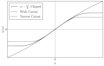
Figure 1: Some $\psi$ functions satisfying Catoni’s constraints (3)

Suppose we have an initial estimate $\mu_{0}$ that has small big-O error, but with a large constant factor—say, the median-of-means estimate on an initial sample of $\xi n$ points for a small constant $\xi$. This will have error $O_{\xi}\left(\sigma\sqrt{\frac{\log\frac{1}{\delta}}{n}}\right)$, which we would like to drive down to $OPT_{1}=\sigma\sqrt{\frac{2\log\frac{1}{\delta}}{n}}$. The final estimate is

$$\widehat{\mu}=\mu_{0}+\frac{1}{n}\sum_{i=1}^{n}T\psi\left(\frac{x_{i}-\mu_{0}}{T}\right)$$ (4)

Intuitively, $T$ is the threshold for being an outlier: if $|x|\ll T$ always, then Bernstein’s inequality will give that the empirical mean achieves $(1+o(1))OPT_{1}$. And indeed, $T\psi(x/T)\approx x$ for $|x|\ll T$, so the estimate (4) is close to the empirical mean in this case. On the other hand, elements $|x|\gg T$ will only be sampled $o(\log\frac{1}{\delta})$ times by Chebyshev’s inequality, so the sample of such events is completely unreliable for $1-\delta$ failure probability; the influence of such elements on the estimator (4) is negligible. The challenge is to handle the cases of $|x|=\Theta(T)$.

The natural approach to show that $\widehat{\mu}$ concentrates about $\mu$ is to bound its moment generating function (MGF). The conditions (3) are precisely what are needed: $\operatorname*{\mathbb{E}}[\exp(\frac{n}{T}\widehat{\mu})]$ depends on $\operatorname*{\mathbb{E}}[\exp(\psi((x-\mu)/T))]$, which is controlled by just the mean and variance of $x$ through (3). As we show in Lemma A.2, this leads to the concentration bound

$$|\widehat{\mu}-\mu|\leq\left(1+O\left(\frac{\log\frac{1}{\delta}}{n}\right)\right)OPT_{1}$$

with probability $1-\delta$.

The estimator (4) we analyze in Appendix A is different from the original Catoni estimator in that Catoni finds a root of $\psi(\frac{x-\mu}{T})$, while our variant approximates this root with essentially one step of Newton’s method. Our analysis does not handle reuse of samples, so it requires the initial estimate $\mu_{0}$ to use a small initial sample. This makes our analysis simpler than [Cat12], which is helpful for the extension we need to get the better constant for $d=2$.

A better constant for “inlier-light” distributions.

The error of the estimate $\widehat{\mu}$ is bounded by the constraints (3). So with a better bound, the estimate would sharpen by a constant factor. In particular, if we could find a $\psi$ with

$$-\log\left(1-x+(1-\eta)\frac{x^{2}}{2}\right)\leq\psi(x)\leq\log\left(1+x+(1-\eta)\frac{x^{2}}{2}\right)$$ (5)

then the variance term which appears in the MGF argument above would have a leading $(1-\eta)$ factor, giving a better constant. Unfortunately, (3) is not achieved by any function $\psi$ for all $x$ simultaneously: both the upper and lower constraints (3) were $x-x^{3}/6\pm\Theta(x^{4})$, so for any $\eta>0$ if $x$ is small enough, shifting the constraints closer by $\Theta(x^{2})$ is impossible.

But, for any $\beta>0$, if we restrict attention to $x$ such that $|x|>\beta$, the constraints of (3) do not exactly match, so there exists an $\eta$ for which (5) is possible for all $|x|>\beta$. We have already discussed one function satisfying tightened constraint: $\psi(x)=x-x^{3}/6$ for $|x|\leq\sqrt{2}$ and $\psi(x)=\left(\sqrt{2}-\frac{2\sqrt{2}}{6}\right)\text{sign}(x)$ otherwise. This is plotted in Figure 1.

As a result of this improved analysis, the Catoni estimate (4) is a constant factor better at handling the variance caused by $x$ whenever $|x|\gtrsim T$.

To formalize this idea, for any constants $\beta,L>0$, we say a distribution is “$(\beta,L)$-inlier-light” if it has at most $(1-L)\sigma^{2}$ variance from elements smaller than $\beta T$. Catoni gets the tight constant on the $(1-L)\sigma^{2}$ variance from inliers, and a better constant on the remaining at-most-$L\sigma^{2}$ variance. Thus it gets error $(1-\tau)OPT_{1}$ error on inlier-light distributions, for some constant $\tau$ depending on $\beta$ and $L$.

An alternative to Catoni for outlier-light distributions.

On the other hand, if a distribution is not inlier-light, it can have very few outliers: there’s at most $L\sigma^{2}$ variance remaining to come from outliers. If we trim at a threshold $\alpha T$ for $\alpha>\beta$, then the contribution to the mean from the trimmed outliers is small: the worst-case is when they are all at the threshold $\alpha T$, in which case the contribution is $\frac{L\sigma^{2}}{\alpha^{2}T^{2}}\cdot\alpha T=\frac{L}{\alpha}OPT_{1}$. And for small $\alpha$, Bernstein’s inequality says that the empirical mean of the untrimmed inliers will have accuracy $(1+O(\alpha))OPT_{1}$. As a result, the trimmed mean, trimmed to $\alpha T$, achieves $(1+O(\alpha+L/\alpha))OPT_{1}$ on distributions that are not $(\beta,L)$ inlier-light, for any $\alpha>\beta$.

Note also that the property of being inlier-light can be tested with $1-\delta$ accuracy, since it involves measuring the variance from bounded entries, as long as $L\gtrsim\beta$. So for $L=\Theta(\beta)$, we can (1) test for inlier-lightness, and on non-inlier-light distributions (2) trim at $\alpha=\sqrt{\beta}$ to get $(1+O(\sqrt{\beta}))OPT_{1}$ error.

Handling $d=2$.

Per the above, in one dimension either the Catoni estimate achieves a constant better than 1, or the trimmed mean achieves constant close to 1. The latter is promising because the empirical mean, in the subgaussian case where it works, gets error $OPT_{1}$ independent of the dimension.

Our $d=2$ algorithm is as follows. We test whether the distribution is inlier-light in either direction $e_{1}$ or $e_{2}$; if it is, we run Catoni on every $1$d projection in a fine net around the circle, and take the center of the minimum enclosing ball of the possible means. In general, this gets at most $JUNG_{2}\cdot OPT_{1}$ error; but the tight instance for Jung is an equilateral triangle, and this error only happens if Catoni gets error bound $OPT_{1}$ in three directions approximately $120^{\circ}$ apart. If the distribution is inlier-light in some direction $e_{i}$, then it is also inlier-light (with slight loss in parameters) in at least one of the triangle directions, so Catoni gets a better error in that direction and a more accurate estimate overall.

On the other hand, if the distribution is not inlier-light in either the $e_{1}$ or $e_{2}$ direction, we remove any element larger than $\sqrt{\beta}T$ in either direction and take the empirical mean of all other samples. This gets error $(1+O(\sqrt{\beta}))OPT_{1}$, without any dependence on $JUNG_{2}$.

For small enough constant $\beta$ and $L=\Theta(\beta)$, either situation will give a constant better than $JUNG_{2}$. Finally, as stated before, we can lift our two-dimensional estimate to higher dimensions using a generalization of Jung’s theorem (Theorem E.2, [Hen92]) to obtain a constant better than $JUNG_{d}$ in $d$-dimensions.

2.2 Robust Estimation, Lower Bound

Now, we discuss the ideas behind Theorem 1.2, showing that the naive strategy of combining one-dimensional estimates is optimal for the robust estimation setting.

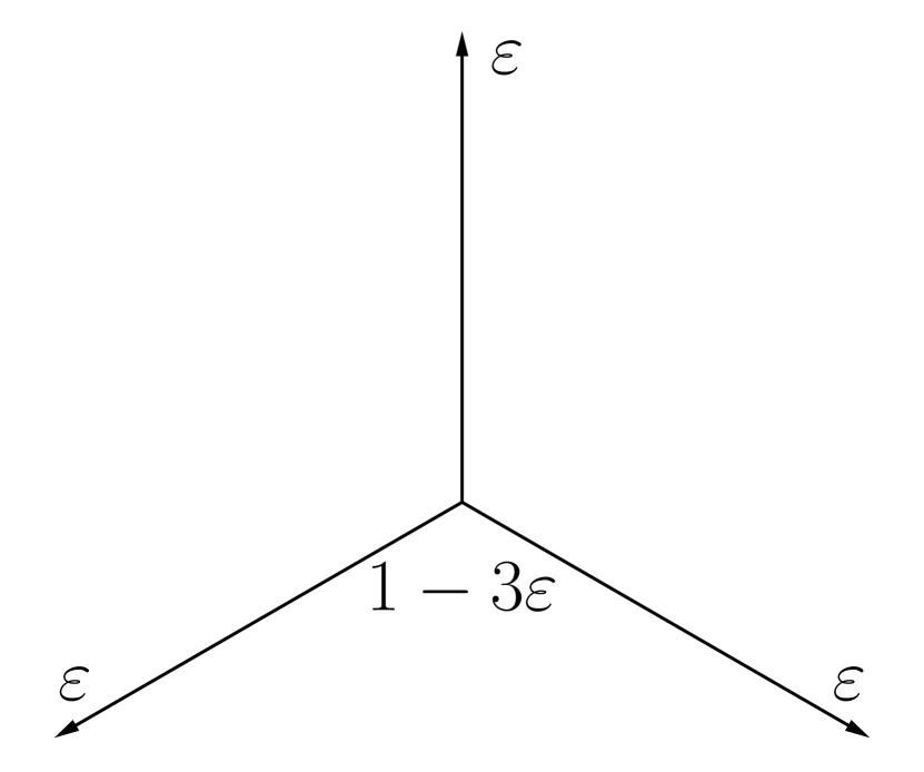
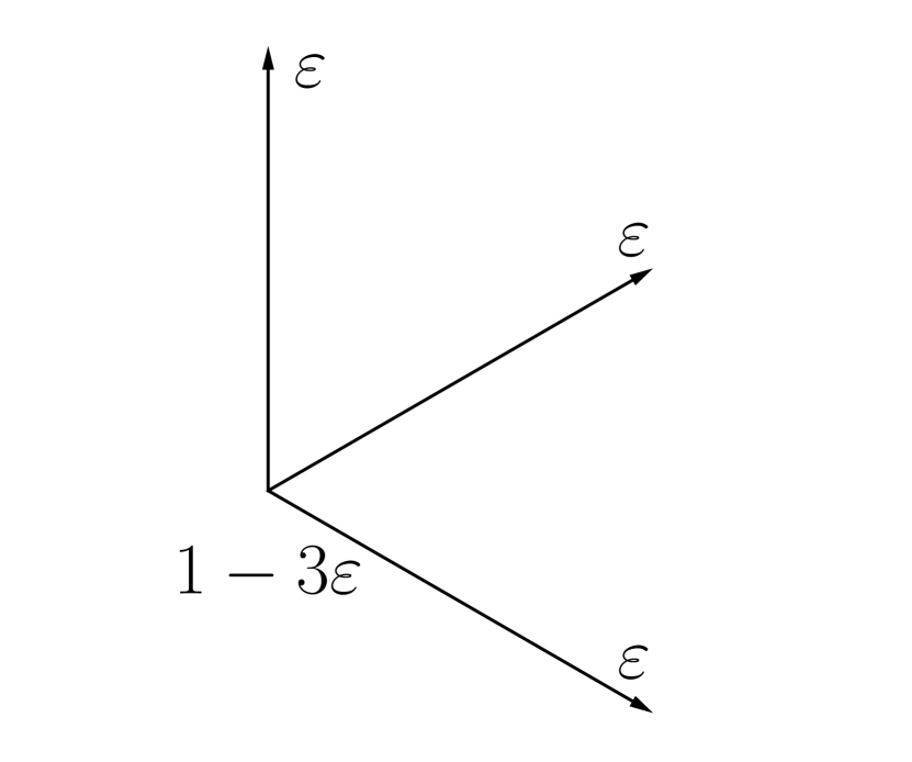
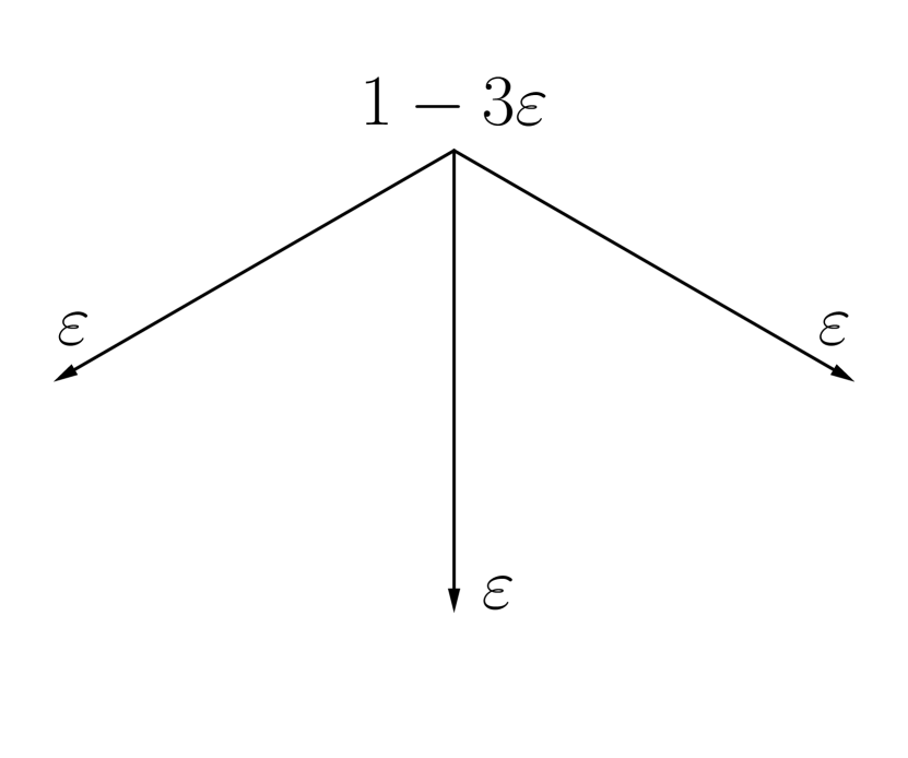
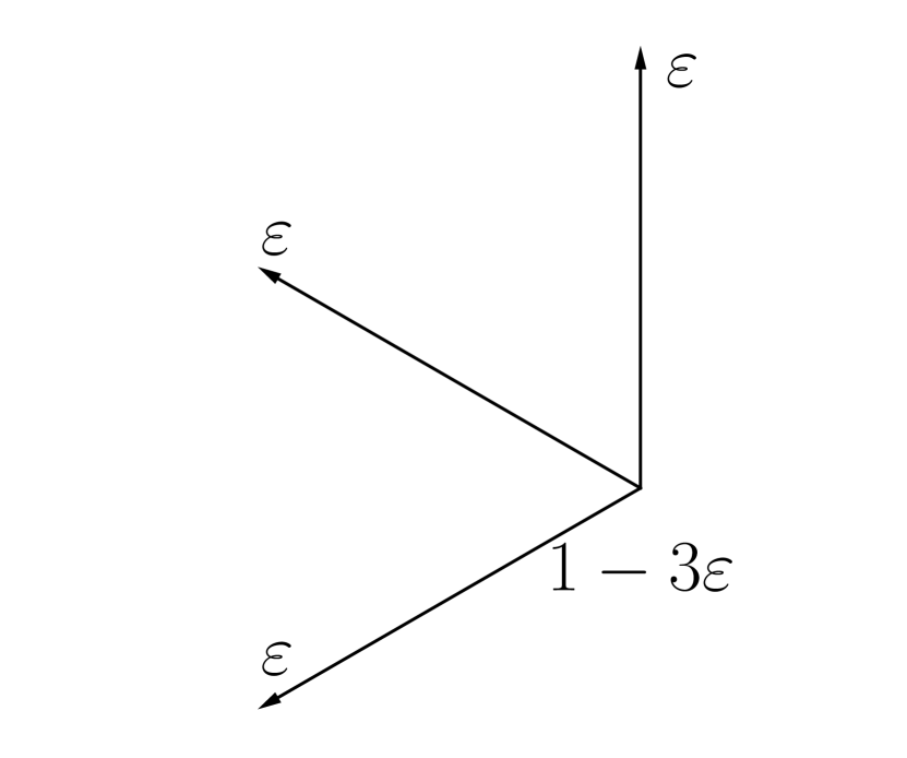
Figure 2: For $d=2$, the algorithm sees as input the distribution on the left after the adversary corrupts $\varepsilon$-mass. The three distributions to its right are ones consistent with the input.

We first show the lower bound for $\varepsilon\leq\frac{1}{d+1}$. The hard instance is that the adversary hands over a distribution that puts $\varepsilon$ mass on each vertex of the regular simplex. The true distribution is the same, but with one of the vertices reflected across the origin. These distributions are all consistent with the observed distribution – that is, they have total variation at most $\varepsilon$ to the distribution handed to us by the adversary – but have means at vertices of a simplex. A regular simplex is the setting where Jung’s theorem is tight, and some calculation gives a $JUNG_{d}\cdot\sqrt{2\varepsilon}$ lower bound.

When $d>\frac{1}{\varepsilon}-1$, we instead restrict to a lower-dimensional space of dimension $d^{\prime}=\lfloor\frac{1}{\varepsilon}-1\rfloor$ and apply the same bound to get a $JUNG_{d^{\prime}}$ lower bound. Since $d^{\prime}$ is large, both $JUNG_{d}$ and $JUNG_{d^{\prime}}$ are $\sqrt{2}-O(\varepsilon)$.

3 Proof Details – Heavy-Tailed Estimator

Here, we provide a detailed description of our heavy-tailed estimator, along with key lemmas in the proof of our main result, Theorem 1.1. We will focus on our $2$-dimensional estimator that achieves a constant better than $JUNG_{2}$; as stated earlier, we can “lift” it to high-dimensions to obtain a constant better than $JUNG_{d}$ in $d$ dimensions. We begin with the formal definition of “inlier-light” and “outlier-light” distributions.

3.1 “Inlier-Light” and “Outlier-Light” Distributions

Definition 3.1 ($(\beta,L)$-Inlier-Light Distribution).

A distribution $x$ over $\mathbb{R}$ with variance at most $\sigma^{2}$ is “$(\beta,L)$-inlier-light” if:

$$\operatorname*{\mathbb{E}}\left[(x-\mu)^{2}\mathbbm{1}_{|x-\mu|\leq\beta T}\right]<(1-L)\sigma^{2}$$

for $T=\sigma\sqrt{\frac{n}{2\log\frac{2}{\delta}}}$.

That is, a distribution is $(\beta,L)$-inlier-light if at most $(1-L)$ fraction of its variance comes from “inlier” points, points within $\beta T$ of $\mu$. We define outlier-light analogously:

Definition 3.2 ($(\beta,L)$-Outlier-Light Distribution).

A distribution $x$ over $\mathbb{R}$ with variance at most $\sigma^{2}$ is “$(\beta,L)$-outlier-light” if:

$$\operatorname*{\mathbb{E}}\left[(x-\mu)^{2}\mathbbm{1}_{|x-\mu|\geq\beta T}\right]<L\sigma^{2}$$

for $T=\sigma\sqrt{\frac{n}{2\log\frac{2}{\delta}}}$.

A distribution $x$ over $\mathbb{R}^{d}$ is $(\beta,L)$-outlier-light if $\langle x,w\rangle$ is $(\beta,L)$-outlier-light for all unit vectors $w$.

3.2 Estimator for One-Dimensional Inlier-Light Distributions

We first show that a variant of Catoni’s Estimator for one-dimensional distributions, when computed using an appropriate $\psi$ function, achieves a rate strictly better than $\sigma\sqrt{\frac{2\log\frac{1}{\delta}}{n}}$, the Gaussian rate, when the distribution is inlier-light. CatoniEstimatorLocal takes an initial estimate $\mu_{0}$ of the mean $\mu$ as input, such that $|\mu_{0}-\mu|\leq O\left(\sigma\sqrt{\frac{\log\frac{1}{\delta}}{n}}\right)$, typically computed using the median-of-means estimator [Dar83].

Algorithm 1 CatoniEstimatorLocal

Input parameters:

• Failure probability $\delta$, One-dimensional iid samples $x_{1},\dots,x_{n}$, Initial estimate $\mu_{0}$, $\psi$ function, Scaling parameter $T$.

1. Compute

   $$r(\mu_{0})=\frac{T}{n}\sum_{i=1}^{n}\psi\left(\frac{x_{i}-\mu_{0}}{T}\right)$$

2. Return mean estimate $\widehat{\mu}=r(\mu_{0})+\mu_{0}$

We will suppose that our $\psi$ function satisfies the following.

Assumption 3.3.

$\psi$ satisfies that for all $x$,

$$-\log\left(1-x+\frac{x^{2}}{2}\right)\leq\psi(x)\leq\log\left(1+x+\frac{x^{2}}{2}\right)$$

Additionally, for constants $0<\beta,\eta<1$, for all $|x|\geq\frac{\beta}{2}$,

$$-\log\left(1-x+(1-\eta)\frac{x^{2}}{2}\right)\leq\psi(x)\leq\log\left(1+x+(1-\eta)\frac{x^{2}}{2}\right)$$

Recall that the “$x-\frac{x^{3}}{6}$, Clipped” function from Figure 1 satisfies that there exists an $\eta$ such that the above is satisfied for every $\beta$. We show that for $(\beta,L)$-inlier-distributions, CatoniEstimatorLocal improves upon the Gaussian rate by a $\approx\left(1-\frac{\eta L}{4}\right)$-factor when using a $\psi$ function satisfying the above, given an initial estimate $\mu_{0}$ of the mean.

Lemma 3.4 (Improved Rate for One-Dimensional Inlier-Light Distributions).

For every constant $0<\beta,L<1$, $C_{1}>1$ there exists constant $C_{2}>1$ such that the following holds. Suppose $\psi$ satisfies Assumption 3.3, $n>C_{2}\log\frac{1}{\delta}$, and we have an initial estimate $\mu_{0}$ with $|\mu_{0}-\mu|\leq C_{1}\sigma\sqrt{\frac{\log\frac{1}{\delta}}{n}}$. We let $T=\sigma\sqrt{\frac{n}{2\log\frac{2}{\delta}}}$.

Given $n$ one-dimensional iid samples $x_{1},\dots,x_{n}$ with mean $\mu$ and variance at most $\sigma^{2}$, if $x_{i}$ is $(\beta,L)$-inlier-light, then, with probability $1-\delta$, the output $\widehat{\mu}$ of Algorithm CatoniEstimatorLocal satisfies

$$\left|\widehat{\mu}-\mu\right|\leq\left(1-\frac{\eta L}{4}+C_{2}\frac{\log\frac{1}{\delta}}{n}\right)\cdot\sigma\cdot\sqrt{\frac{2\log\frac{2}{\delta}}{n}}$$

3.3 Testing Inlier-Light vs. Outlier-Light

Our strategy will be to first test whether our two-dimensional samples come from a distribution that is inlier-light, or outlier-light, and use an appropriate estimator accordingly. Our tester (Algorithm 2DInlierOutlierLightTesting, described in Appendix B.2) takes in $n$ samples along with initial estimates $\mu_{0}^{e_{1}},\mu_{0}^{e_{2}}$ of the mean in directions $e_{1},e_{2}$ respectively, and either identifies a direction $e_{j}$ in which the distribution is inlier-light, or certifies that the distribution is outlier-light in every direction. Formally,

Lemma 3.5 (Two-dimensional Inlier-Light vs. Outlier-Light Test).

For every constant $\beta<\frac{1}{8}$, $L>8\beta$, and $C_{1}>1$, there exists constant $C_{2}>1$ such that the following holds. Suppose $n>C_{2}\log\frac{1}{\delta}$ and suppose our initial estimates $\mu_{0}^{e_{j}}$ satisfy $|\mu_{0}^{e_{j}}-\langle e_{j},\mu\rangle|\leq C_{1}\sigma\sqrt{\frac{\log\frac{1}{\delta}}{n}}$ for $j\in\{1,2\}$. We let $T=\sigma\sqrt{\frac{n}{2\log\frac{4}{\delta}}}$.

Given $n$ two-dimensional iid samples $x_{1},\dots,x_{n}$ with mean $\mu$ and covariance $\Sigma\preccurlyeq\sigma^{2}I_{2}$, with probability $1-\delta$, Algorithm 2DInlierOutlierLightTester satisfies the following.

• If the output is $e_{j}$, $\langle e_{j},x_{i}\rangle$ is $(\beta,L)$-inlier-light

• If the output is $\perp$, $x_{i}$ is $\left(16\beta,16L\right)$-outlier-light. (That is, $\langle x_{i},w\rangle$ is $\left(16\beta,16L\right)$-outlier-light for all unit vectors $w$.)

3.4 Catoni-Based Estimator for Two-Dimensional Inlier-Light Distributions

We recall the standard definition of a $\rho$-net of vectors over $\mathbb{R}^{2}$:

Assumption 3.6.

$U$ is a $\rho$-net of $O(1/\rho)$ unit vectors such that for every $v\in\mathbb{S}^{1}$, there exists a vector $u\in U$ with $\|v-u\|\leq\rho$.

If our distribution over $\mathbb{R}^{2}$ is determined to be inlier-light in some direction $e_{j}$, we will make use of the following $2$-dimensional estimator.

Algorithm 2 2DInlierLightEstimator

Input parameters:

• Failure probability $\delta$, Two-dimensional iid samples $x_{1},\dots,x_{n}$, $\psi$ function, Scaling parameter $T$, Inlier-Outlier-Ligtness parameters $\beta,L$, Approximation parameters $0<\xi,\tau<1$, Set of unit vectors $U$, Initial estimates $\mu_{0}^{u}$ for $u\in U$.

1. For every $u\in U$, run Algorithm 1DInlierOutlierTester with samples $\langle u,x_{1}\rangle,\dots,\langle u,x_{n}\rangle$, Failure probability $\frac{\delta}{4|U|}$, initial estimate $\mu_{0}^{u}$, and Lightness parameters $\beta/32,L/32$. If the output is “INLIER-LIGHT”, let $\alpha_{u}=1-\Theta(\tau)$. Otherwise, let $\alpha_{u}=1+\xi$.

2. For every $u\in U$, run Algorithm CatoniEstimatorLocal with samples $\langle u,x_{1}\rangle,\dots,\langle u,x_{n}\rangle$, initial estimate $\mu_{0}^{u}$, and failure probability $\frac{\delta}{4|U|}$ and let the mean estimate obtained be $\widehat{\mu}_{u}$.

3. For each $u\in U$, define set $S_{u}=\left\{w:|\langle u,w\rangle-\widehat{\mu}_{u}|\leq\alpha_{u}\cdot\sigma\sqrt{\frac{2\log\frac{2}{\delta}}{n}}\right\}$. Let $S$ be the convex set given by $S:=\cap_{u\in U}S_{u}$.

4. Consider the minimum enclosing ball of set $S$ and return its center as the mean estimate $\widehat{\mu}$.

2DInlierLightEstimator takes in a $\rho$-net $U$, in addition to the iid samples $x_{1},\dots,x_{n}\in\mathbb{R}^{2}$ and failure probability $\delta$. For each net vector $u\in U$, it tests whether the distribution of the $\langle u,x_{i}\rangle$ is inlier-light, computes an estimate of the mean in direction $u$ using our $1$-d estimator for inlier-light distributions, and assigns a confidence interval accordingly. The final estimate $\widehat{\mu}$ is the center of the minimum enclosing ball of the points that satisfy all $|U|$ confidence intervals. We show:

Lemma 3.7 (Two-Dimensional Estimator for Inlier-Light Distributions).

For every constant $0<\beta<1/32,L>32\beta$, and $C>1$, there exist constants $\xi,\tau<1$ such that the following holds. Suppose $n>O_{\xi}\left(\log\frac{1}{\delta}\right)$, and we have that $|\mu_{0}^{u}-\langle u,\mu\rangle|\leq C\sigma\sqrt{\frac{\log\frac{1}{\delta}}{n}}$ for all $u\in U$. Suppose further that $\psi$ satisfies Assumption 3.3 for parameter $\beta/8$ and that $U$ satisfies Assumption 3.6 for $\rho=\delta^{\Theta(\xi)}$. Let $T=\sigma\sqrt{\frac{n}{2\log\frac{2}{\delta}}}$.

Given $n$ two-dimensional iid samples $x_{1},\dots,x_{n}$ with mean $\mu$ and covariance $\Sigma\preccurlyeq\sigma^{2}I_{2}$ such that $\langle e_{k},x_{i}\rangle$ is $(\beta,L)$-inlier-light, with probability $1-\delta$, Algorithm 2DInlierLightEstimator returns a mean estimate $\widehat{\mu}$ with

$$\|\widehat{\mu}-\mu\|\leq(1-\tau)\cdot JUNG_{2}\cdot\sigma\sqrt{\frac{2\log\frac{2}{\delta}}{n}}$$

3.5 Trimmed-Mean-Based Estimator for Two-Dimensional Outlier-Light Distributions

Algorithm 3 2DOutlierLightEstimator

Input parameters:

• Failure probability $\delta$, Two-dimensional samples $x_{1},\dots,x_{n}$, Initial estimates $\mu_{0}^{e_{1}},\mu_{0}^{e_{2}}$, Scaling parameter $T$, Approximation parameters $0<\beta,\xi<1$.

1. Consider the subset of samples $X^{\prime}$ obtained by throwing out any sample $x_{i}$ with $|\langle e_{j},x_{i}\rangle-\mu_{0}^{e_{j}}|>\sqrt{\beta}T$ for either $e_{1}$ or $e_{2}$. Return estimate $\widehat{\mu}=\frac{1}{n}\sum_{i\in X^{\prime}}x_{i}$.

For outlier-light distributions, 2DOutlierLightEstimator computes a simple trimmed-mean estimate, throwing out any point more than $\sqrt{\beta}T$ away from the initial mean estimate in the $e_{1},e_{2}$ directions.

Lemma 3.8 (Two-Dimensional Estimator for Outlier-Light Distributions).

Define $T=\sigma\sqrt{\frac{n}{2\log\frac{2}{\delta}}}$. For any constant $\beta<1$, let $x_{1},\dots,x_{n}$ be iid samples from a two-dimensional $(\beta,O(\beta))$-outlier-light distribution with mean $\mu$ and covariance $\Sigma\preccurlyeq\sigma^{2}I_{2}$. Then, the output of Algorithm 2DOutlierLightEstimator when given as input initial estimates $\mu_{0}^{j}$ satisfying $|\mu_{0}^{j}-\langle e_{j},\mu\rangle|\leq O\left(\sigma\sqrt{\frac{\log\frac{1}{\delta}}{n}}\right)$ outputs estimate $\widehat{\mu}$ satisfying with probability $1-\delta$,

$$\|\widehat{\mu}-\mu\|\leq\left(1+O\left(\sqrt{\beta}\right)\right)\cdot OPT_{1}$$

3.6 Final Two-Dimensional Estimator

Finally, we put together the previous parts to obtain our final Algorithm 2DHeavyTailedEstimator.

Algorithm 4 2DHeavyTailedEstimator

Input parameters:

• Failure probability $\delta$, Two-dimensional samples $x_{1},\dots,x_{n}$, $\psi$ function, Scaling parameter $T$, Inlier-Outlier-Lightness parameters $\beta,L$, Approximation parameters $0<\xi,\tau<1$, set of unit vectors $U$

1. Using $\Theta(\xi)n$ samples, compute Median-of-Means estimates $\mu_{0}^{e_{j}}$ of the one-dimensional samples $\langle e_{j},x_{i}\rangle$ with failure probability $\frac{\delta}{4(|U|+2)}$ for each $j\in\{1,2\}$.

2. Using $\Theta(\xi)n$ samples, compute Median-of-Means estimates $\mu_{0}^{u}$ of the one-dimensional samples $\langle u,x_{i}\rangle$ with failure probability $\frac{\delta}{4(|U|+2)}$ for each $u\in U$.

3. Let the set of the remaining $(1-\Theta(\xi))n$ samples be $X^{\prime}$. Run Algorithm 2DInlierOutlierLightTester using failure probability $\delta/4$, the samples in $X^{\prime}$ and initial estimates $\mu_{0}^{e_{1}},\mu_{0}^{e_{2}}$.

4. If the output of 2DInlierOutlierLightTester is some $e_{j}$, run 2DInlierLightEstimator using failure probability $\delta/8$, the samples in $X^{\prime}$, and the initial estimates $\mu_{0}^{u}$, and output its mean estimate $\widehat{\mu}$.

5. If instead the output of 2DInlierOutlierLightTester is $\perp$, run 2DOutlierLightEstimator using failure probability $\delta/4$, the samples in $X^{\prime}$ and initial estimates $\mu_{0}^{e_{1}},\mu_{0}^{e_{2}}$. Return its output $\widehat{\mu}$.

Theorem 3.9 (Final Two-Dimensional Estimator).

For any sufficiently small constant $\tau>0$, there exist constants $0<\xi,\beta,L<1$ such that the following holds. Suppose $n>O_{\xi}(\log\frac{1}{\delta})$ and $T=\sigma\sqrt{\frac{n}{2\log\frac{2}{\delta}}}$. Suppose the set $U$ is a $\rho$-net, satisfying Assumption 3.6 for $\rho=\delta^{\Theta(\xi)}$.

Given $n$ two-dimensional samples $x_{1},\dots,x_{n}$ with mean $\mu$ and covariance $\Sigma\preccurlyeq\sigma^{2}I_{2}$, with probability $1-\delta$, Algorithm 2DHeavyTailedEstimator returns an estimate $\widehat{\mu}$ with

$$\|\widehat{\mu}-\mu\|\leq(1-\tau)\cdot JUNG_{2}\cdot\sigma\sqrt{\frac{2\log\frac{2}{\delta}}{n}}$$

Proof.

First note that by classical results on Median-of-Means [Dar83] and a union bound, for every vector $v\in U\cup\{e_{1},e_{2}\}$, we have with probability $1-\delta/4$,

$$\left|\mu_{0}^{v}-\langle v,\mu\rangle\right|\leq O\left(\sigma\sqrt{\frac{\log\frac{1}{\delta}}{n}}\right)$$

since $n>O_{\xi}(\log\frac{1}{\delta})$. For the remaining proof, we condition on the above. Now, by a union bound, there exist constants $0<\beta,L<1$, such that by Lemmas 3.5, 3.7 and 3.8, the following events happen with probability $1-3\delta/4$.

• If the output of Algorithm 2DInlierOutlierLightTester is $e_{j}$, $\langle e_{j},x_{i}\rangle$ is $(\beta,L)$-inlier-light. On the other hand, if the output is $\perp$, $x_{i}$ is $(8\beta,8L)$-outlier-light.

• If $\langle e_{j},x_{i}\rangle$ is $(\beta,L)$-inlier-light, Algorithm 2DInlierLightEstimator returns $\widehat{\mu}$ with

  $$\|\widehat{\mu}-\mu\| \leq(1-2\tau+\Theta(\xi))\cdot JUNG_{2}\cdot\sigma\sqrt{\frac{2\log\frac{2}{\delta}}{n}}$$

  $$\leq(1-\tau)\cdot JUNG_{2}\cdot\sigma\sqrt{\frac{2\log\frac{2}{\delta}}{n}}$$

• If $x_{i}$ is $(8\beta,8L)$-outlier-light, for $L=O(\beta)$, Algorithm 2DOutlierLightEstimator returns $\widehat{\mu}$ with

  $$\|\widehat{\mu}-\mu\|\leq\left(1+O\left(\sqrt{\beta}\right)\right)\cdot\sigma\sqrt{\frac{2\log\frac{1}{\delta}}{n}}$$

So, with probability $1-\delta$ in total, for $\beta$ small enough, Algorithm 2DHeavyTailedEstimator returns estimate $\widehat{\mu}$ with

$$\|\widehat{\mu}-\mu\|\leq(1-\tau)\cdot JUNG_{2}\cdot\sigma\sqrt{\frac{2\log\frac{2}{\delta}}{n}}$$

∎

4 Open Questions

Our work suggests a number of exciting avenues for future research. Some of these are:

• What is the sharp rate for heavy tailed estimation when $\log\frac{1}{\delta}\gg d$? Our work establishes that it is not achieved by the naive strategy of aggregating one-dimensional estimates. Is it possible to achieve the Gaussian rate?

• Our upper and lower bounds are statistical—what about polynomial-time estimation? What are the sharp constants achievable, and is there a computational-statistical tradeoff? In particular, for large $d$ no estimator achieving even the $JUNG_{d}\approx\sqrt{2}$ factor loss is known—current polynomial-time estimators [Hop20, CFB19] rely on the median-of-means framework, which loses constants even in one dimension.

• What are the sharp rates for other estimation problems under heavy-tailed noise? For instance, covariance estimation or regression?

Appendix A Vanilla One-Dimensional Catoni Estimator

We first describe a variant of Catoni’s one-dimensional estimator [Cat12] for bounded variance distributions.

Algorithm 1 CatoniEstimatorLocal

Input parameters:

• Failure probability $\delta$, One-dimensional iid samples $x_{1},\dots,x_{n}$, Initial estimate $\mu_{0}$, $\psi$ function, Scaling parameter $T$.

1. Compute

   $$r(\mu_{0})=\frac{T}{n}\sum_{i=1}^{n}\psi\left(\frac{x_{i}-\mu_{0}}{T}\right)$$

2. Return mean estimate $\widehat{\mu}=r(\mu_{0})+\mu_{0}$

Assumption A.1.

$\psi$ satisfies that for all $x$,

$$-\log\left(1-x+\frac{x^{2}}{2}\right)\leq\psi(x)\leq\log\left(1+x+\frac{x^{2}}{2}\right)$$

Lemma A.2.

For every constant $C_{1}>1$ there exists constant $C_{2}>1$ such that the following holds. Suppose $\psi$ satisfies Assumption A.1, $n>C_{2}\log\frac{1}{\delta}$, and we have an initial estimate $\mu_{0}$ with $|\mu_{0}-\mu|\leq C_{1}\sigma\sqrt{\frac{\log\frac{1}{\delta}}{n}}$. We let $T=\sigma\sqrt{\frac{n}{2\log\frac{2}{\delta}}}$. Given $n$ one-dimensional iid samples $x_{1},\dots,x_{n}$ with mean $\mu$ and variance at most $\sigma^{2}$, with probability $1-\delta$, the output $\widehat{\mu}$ of Algorithm CatoniEstimatorLocal satisfies

$$\left|\widehat{\mu}-\mu\right|\leq\left(1+C_{2}\frac{\log\frac{1}{\delta}}{n}\right)\cdot\sigma\cdot\sqrt{\frac{2\log\frac{2}{\delta}}{n}}$$

Proof.

By Assumption A.1, we have

$$\operatorname*{\mathbb{E}}\left[\exp\left(\frac{n}{T}r(\mu_{0})\right)\right] =\prod_{i=1}^{n}\operatorname*{\mathbb{E}}\left[\exp\left(\psi\left(\frac{x_{i}-\mu_{0}}{T}\right)\right)\right]$$

$$\leq\prod_{i=1}^{n}\operatorname*{\mathbb{E}}\left[\left(1+\frac{x_{i}-\mu_{0}}{T}+\frac{(x_{i}-\mu_{0})^{2}}{2T^{2}}\right)\right]$$

$$=\left(1+\frac{\mu-\mu_{0}}{T}+\frac{1}{2T^{2}}\cdot\left[\sigma^{2}+(\mu-\mu_{0})^{2}\right]\right)^{n}$$

$$\leq\exp\left(\frac{n}{T}(\mu-\mu_{0})+\frac{n}{2T^{2}}\cdot\left[\sigma^{2}+(\mu-\mu_{0})^{2}\right]\right)$$

So, by Markov’s inequality, for $T=\sigma\sqrt{\frac{n}{2\log\frac{2}{\delta}}}$, we have

$$\Pr\left[r(\mu_{0})\geq(\mu-\mu_{0})+\sigma\cdot\sqrt{\frac{2\log\frac{2}{\delta}}{n}}\left(1+C_{2}\frac{\log\frac{1}{\delta}}{n}\right)\right]$$

$$\leq\exp\left(\frac{n}{2T^{2}}\cdot\left[\sigma^{2}+(\mu-\mu_{0})^{2}\right]-\frac{n}{T}\cdot\sigma\cdot\sqrt{\frac{2\log\frac{2}{\delta}}{n}}\left(1+C_{2}\frac{\log\frac{1}{\delta}}{n}\right)\right)$$

$$\leq\exp\left(-\log\frac{2}{\delta}\right)$$

$$=\delta/2$$

since $|\mu-\mu_{0}|\leq C_{1}\sigma\sqrt{\frac{\log\frac{1}{\delta}}{n}}$, for $C_{2}\geq\Omega(C_{1}^{2})$.

Similarly, for the lower tail, the MGF is given by

$$\operatorname*{\mathbb{E}}\left[\exp\left(-\frac{n}{T}r(\theta_{0})\right)\right] \leq\prod_{i=1}^{n}\operatorname*{\mathbb{E}}\left[\left(1-\frac{x_{i}-\mu_{0}}{T}+\frac{(x_{i}-\mu_{0})^{2}}{2T^{2}}\right)\right]$$

$$\leq\exp\left(-\frac{n}{T}(\mu-\mu_{0})+\frac{n}{2T^{2}}\left[\sigma^{2}+(\mu-\mu_{0})^{2}\right]\right)$$

So, by Markov’s inequality, for $T=\sigma\cdot\sqrt{\frac{n}{2\log\frac{2}{\delta}}}$, we have

$$\Pr\left[r(\mu_{0})\leq(\mu-\mu_{0})-\sigma\cdot\sqrt{\frac{2\log\frac{2}{\delta}}{n}}\left(1+C_{2}\frac{\log\frac{1}{\delta}}{n}\right)\right]\leq\delta/2$$

Then, taking a union bound gives the claim. ∎

Algorithm 5 CatoniEstimator

Input parameters:

• Failure probability $\delta$, One-dimensional iid samples $x_{1},\dots,x_{n}$, $\psi$ function, Scaling parameter $T$, Approximation parameter $0<\xi<1$.

1. Use the first $\Theta(\xi n)$ samples to compute the Median-of-Means estimate $\mu_{0}$ with failure probability $\delta/2$.

2. Return the result $\widehat{\mu}$ of Algorithm CatoniEstimatorLocal using initial estimate $\mu_{0}$, and the remaining $(1-\Theta(\xi))n$ samples, and failure probability $\delta/2$.

Theorem A.3.

For every constant $\xi>0$, suppose $n>O_{\xi}(\log\frac{1}{\delta})$, $\psi$ satisfies Assumption A.1, and consider $T=\sigma\sqrt{\frac{n}{2\log\frac{4}{\delta}}}$. Given $n$ one-dimensional iid samples $x_{1},\dots,x_{n}$ with mean $\mu$ and variance at most $\sigma^{2}$, with probability $1-\delta$, the output $\widehat{\mu}$ of Algorithm CatoniEstimator satisfies

$$\left|\widehat{\mu}-\mu\right|\leq\left(1+\xi\right)\cdot\sigma\cdot\sqrt{\frac{2\log\frac{4}{\delta}}{n}}$$

Proof.

First, by classical results on Median-of-Means [Dar83], $\mu_{0}$ satisfies with probability $1-\delta/2$,

$$|\mu_{0}-\mu|\leq C\sigma\sqrt{\frac{\log\frac{1}{\delta}}{n\xi}}$$

for some constant $C>0$. Then, invoking Lemma 1 using the remaining $(1-\Theta(\xi))n$ samples and failure probability $\delta/2$ gives the claim. ∎

Appendix B Improved Heavy-Tailed Estimator

We will make use of the following notions of “$(\beta,L)$-inlier-light” and “$(\beta,L)$-outlier-light” distributions throughout this section. See 3.1 See 3.2

B.1 Improved One-Dimensional Catoni-Based Estimator when Inlier-Light

The following assumption on $\psi$ functions is stronger than the Catoni requirement, and allows for a more accurate estimate when a distribution is $(\beta,L)$-inlier-light. See 3.3

There exist $\psi$ functions such that for every $\beta>0$, there exists $\eta>0$ such that Assumption 3.3 is satisfied. One such function is $\psi(x)=x-x^{3}/6$ for $|x|\leq 1$ and $\psi(x)=\frac{5}{6}\text{sign}(x)$ for $|x|>1$. For $|x|\lesssim 1$, there is $\Theta(x^{4})$ flexibility in the choice of $\psi(x)$.

See 3.4

Proof.

By Assumption 3.3, we have

$$\operatorname*{\mathbb{E}}\left[\exp\left(\frac{n}{T}r(\mu_{0})\right)\right]$$

$$=\prod_{i=1}^{n}\operatorname*{\mathbb{E}}\left[\exp\left(\psi\left(\frac{x_{i}-\mu_{0}}{T}\right)\right)\right]$$

$$=\prod_{i=1}^{n}\left(\operatorname*{\mathbb{E}}\left[\exp\left(\psi\left(\frac{x_{i}-\mu_{0}}{T}\right)\right)\mathbbm{1}_{|x_{i}-\mu_{0}|\leq\beta T/2}\right]+\operatorname*{\mathbb{E}}\left[\exp\left(\psi\left(\frac{x_{i}-\mu_{0}}{T}\right)\right)\mathbbm{1}_{|x_{i}-\mu_{0}|>\beta T/2}\right]\right)$$

$$\leq\prod_{i=1}^{n}\left(1+\operatorname*{\mathbb{E}}\left[\frac{x_{i}-\mu_{0}}{T}\right]+\frac{1}{2T^{2}}\left(\operatorname*{\mathbb{E}}\left[\left(x_{i}-\mu_{0}\right)^{2}\mathbbm{1}_{|x_{i}-\mu_{0}|\leq\beta T/2}\right]+(1-\eta)\operatorname*{\mathbb{E}}\left[(x_{i}-\mu_{0})^{2}\mathbbm{1}_{|x_{i}-\mu_{0}|>\beta T/2}\right]\right)\right)$$

Now, since $x_{i}$ is $(\beta,L)$-inlier-light, so that $\operatorname*{\mathbb{E}}\left[(x_{i}-\mu)^{2}\mathbbm{1}_{|x_{i}-\mu|\leq\beta T}\right]<(1-L)\sigma^{2}$, we have

$$\operatorname*{\mathbb{E}}\left[(x_{i}-\mu)^{2}\mathbbm{1}_{|x_{i}-\mu_{0}|\leq\beta T/2}\right]\leq\operatorname*{\mathbb{E}}\left[(x_{i}-\mu)^{2}\mathbbm{1}_{|x_{i}-\mu|\leq\beta T}\right]\leq(1-L)\sigma^{2}$$

since $|\mu-\mu_{0}|\leq O\left(\sigma\sqrt{\frac{\log\frac{1}{\delta}}{n}}\right)\leq\beta T/2$. So,

$$\operatorname*{\mathbb{E}}\left[\left(x_{i}-\mu_{0}\right)^{2}\mathbbm{1}_{|x_{i}-\mu_{0}|\leq\beta T/2}\right]+(1-\eta)\operatorname*{\mathbb{E}}\left[(x_{i}-\mu_{0})^{2}\mathbbm{1}_{|x_{i}-\mu_{0}|>\beta T/2}\right]$$

$$\leq(\mu-\mu_{0})^{2}+\operatorname*{\mathbb{E}}\left[(x_{i}-\mu)^{2}\mathbbm{1}_{|x_{i}-\mu_{0}|\leq\beta T/2}\right]+(1-\eta)\operatorname*{\mathbb{E}}\left[(x_{i}-\mu)^{2}\mathbbm{1}_{|x_{i}-\mu_{0}|>\beta T/2}\right]$$

$$\quad-2\eta\operatorname*{\mathbb{E}}\left[(x_{i}-\mu)(\mu-\mu_{0})\mathbbm{1}_{|x_{i}-\mu_{0}|>\beta T/2}\right]$$

$$\leq\left(1-\frac{\eta L}{2}\right)\sigma^{2}$$

since $n>C_{2}\log\frac{1}{\delta}$. So,

$$\operatorname*{\mathbb{E}}\left[\exp\left(\frac{n}{T}r(\mu_{0})\right)\right] \leq\prod_{i=1}^{n}\left(1+\frac{\mu-\mu_{0}}{T}+\frac{\sigma^{2}}{2T^{2}}\left(1-\frac{\eta L}{2}\right)\right)$$

$$\leq\exp\left(n\cdot\frac{\mu-\mu_{0}}{T}+\frac{n\sigma^{2}}{2T^{2}}\left(1-\frac{\eta L}{2}\right)\right)$$

Then, by Markov’s inequality, for $T=\sigma\sqrt{\frac{n}{2\log\frac{2}{\delta}}}$,

$$\Pr\left[r(\mu_{0})\geq(\mu-\mu_{0})+\left(1-\frac{\eta L}{4}+\frac{C_{2}\log\frac{1}{\delta}}{n}\right)\cdot\sigma\cdot\sqrt{\frac{2\log\frac{2}{\delta}}{n}}\right]$$

$$\leq\exp\left(\frac{n\sigma^{2}}{2T^{2}}\left(1-\frac{\eta L}{2}\right)-\frac{n}{T}\cdot\left(1-\frac{\eta L}{4}+\frac{C_{2}\log\frac{1}{\delta}}{n}\right)\cdot\sigma\cdot\sqrt{\frac{2\log\frac{2}{\delta}}{n}}\right)$$

$$\leq\exp\left(-\log\frac{2}{\delta}\right)$$

$$=\delta/2$$

since $|\mu-\mu_{0}|\leq C_{1}\sigma\sqrt{\frac{2\log\frac{1}{\delta}}{n}}$, for $C_{2}\geq\Omega(C_{1}^{2})$.

Similarly, for the lower tail, the MGF is given by

$$\operatorname*{\mathbb{E}}\left[\exp\left(-\frac{n}{T}r(\mu_{0})\right)\right]\leq\exp\left(-n\cdot\frac{\mu-\mu_{0}}{T}+\frac{n\sigma^{2}}{T^{2}}\left(1-\frac{\eta L}{2}\right)\right)$$

so that by Markov’s inequality,

$$\Pr\left[r(\mu_{0})\leq(\mu-\mu_{0})-\left(1-\frac{\eta L}{4}\right)\cdot\sigma\cdot\sqrt{\frac{2\log\frac{2}{\delta}}{n}}\right]\leq\delta/2$$

for $T=\sigma\sqrt{\frac{n}{2\log\frac{2}{\delta}}}$.

Taking a union bound gives the claim. ∎

B.2 Testing Inlier-Light vs. Outlier-Light

Algorithm 6 1DInlierOutlierLightTester

Input parameters:

• Failure Probability $\delta$, One-dimensional iid samples $x_{1},\dots,x_{n}$, Scaling parameter $T$, Inlier-Outlier-Lightness parameters $\beta,L$, Initial estimate $\mu_{0}$.

1. Compute

   $$B=\frac{1}{n}\sum_{i=1}^{n}(x_{i}-\mu_{0})^{2}\mathbbm{1}_{|x_{i}-\mu_{0}|\leq 2\beta T}$$

2. If $B\leq\left(1-2L\right)\sigma^{2}$, return “INLIER-LIGHT”. Otherwise return “OUTLIER-LIGHT”.

Lemma B.1.

For every constant $\beta<1/16,L>16\beta$ and $C_{1}>1$, there exists constant $C_{2}>1$ such that the following holds. Suppose $n>C_{2}\log\frac{1}{\delta}$, and we have that $|\mu_{0}-\mu|\leq C_{1}\sigma\sqrt{\frac{\log\frac{1}{\delta}}{n}}$. We let $T=\sigma\sqrt{\frac{n}{2\log\frac{2}{\delta}}}$.

Given $n$ one-dimensional iid samples $x_{1},\dots,x_{n}$, with mean $\mu$ and variance at most $\sigma^{2}$, with probability $1-\delta$, we have that

• If Algorithm 1DInlierOutlierLightTester returns “INLIER-LIGHT”, then $x_{i}$ is $(\beta,L)$-inlier-light,

• If Algorithm 1DInlierOutlierLightTester returns “OUTLIER-LIGHT”, then $x_{i}$ is $(4\beta,4L)$-outlier-light

Proof.

First, note that the variance of $(x_{i}-\mu)^{2}\mathbbm{1}_{|x_{i}-\mu|\leq\beta T}$ is at most $(\beta T\sigma)^{2}$, and it is bounded by $(\beta T)^{2}$. Thus, by Bernstein’s inequality, since $T=\sigma\sqrt{\frac{n}{2\log\frac{2}{\delta}}}$ and $L>8\beta$, with probability $1-\delta$,

$$\left|\frac{1}{n}\sum_{i=1}^{n}(x_{i}-\mu)^{2}\mathbbm{1}_{|x_{i}-\mu|\leq\beta T}-\operatorname*{\mathbb{E}}\left[(x-\mu)^{2}\mathbbm{1}_{|x-\mu|\leq\beta T}\right]\right| \leq\beta T\sigma\sqrt{\frac{2\log\frac{2}{\delta}}{n}}+2(\beta T)^{2}\frac{\log\frac{2}{\delta}}{n}$$

$$=2\beta\sigma^{2}\leq L\sigma^{2}/4$$

and

$$\left|\frac{1}{n}\sum_{i=1}^{n}(x_{i}-\mu)^{2}\mathbbm{1}_{|x_{i}-\mu|\leq 4\beta T}-\operatorname*{\mathbb{E}}\left[(x-\mu)^{2}\mathbbm{1}_{|x-\mu|\leq 4\beta T}\right]\right| \leq 4\beta T\sigma\sqrt{\frac{2\log\frac{2}{\delta}}{n}}+8(\beta T)^{2}\frac{\log\frac{2}{\delta}}{n}$$

$$=8\beta\sigma^{2}\leq L\sigma^{2}$$

We condition on the above. Now, since $|\mu_{0}-\mu|\leq C_{1}\sigma\sqrt{\frac{\log\frac{1}{\delta}}{n}}\leq\frac{\beta T}{2}$, we have

$$(x_{i}-\mu_{0})^{2}\mathbbm{1}_{|x_{i}-\mu|\leq\beta T}\leq(x_{i}-\mu_{0})^{2}\mathbbm{1}_{|x_{i}-\mu_{0}|\leq 2\beta T}$$

So, since $|\mu-\mu_{0}|\leq C_{1}\sigma\sqrt{\frac{\log\frac{1}{\delta}}{n}}$, we have, by Cauchy-Schwarz,

$$\frac{1}{n}\sum_{i=1}^{n}(x_{i}-\mu)^{2}\mathbbm{1}_{|x_{i}-\mu|\leq\beta T}$$

$$\leq\frac{1}{n}\sum_{i=1}^{n}(x_{i}-\mu_{0})^{2}\mathbbm{1}_{|x_{i}-\mu_{0}|\leq 2\beta T}+C_{1}^{2}\sigma^{2}\frac{\log\frac{1}{\delta}}{n}+2C_{1}\sigma\sqrt{\frac{\log\frac{1}{\delta}}{n}}\cdot\sqrt{\frac{1}{n}\sum_{i=1}^{n}(x_{i}-\mu_{0})^{2}\mathbbm{1}_{|x_{i}-\mu_{0}|\leq 2\beta T}}$$

So, if Algorithm 1DInlierOutlierLightTester returns “INLIER-LIGHT” so that $\frac{1}{n}\sum_{i=1}^{n}(x_{i}-\mu_{0})^{2}\mathbbm{1}_{|x_{i}-\mu_{0}|\leq 2\beta T}\leq\left(1-2L\right)\sigma^{2}$, then,

$$\frac{1}{n}\sum_{i=1}^{n}(x_{i}-\mu)^{2}\mathbbm{1}_{|x_{i}-\mu|\leq\beta T} \leq\left(1-\frac{3L}{2}\right)\sigma^{2}$$

for $C_{2}$ large enough. So, in this case

$$\operatorname*{\mathbb{E}}\left[(x-\mu)^{2}\mathbbm{1}_{|x-\mu|\leq\beta T}\right]\leq\left(1-L\right)\sigma^{2}$$

so that $x_{i}$ is $(\beta,L)$-inlier-light, as claimed. For the other case, note that

$$(x_{i}-\mu_{0})^{2}\mathbbm{1}_{|x_{i}-\mu|\leq 4\beta T}\geq(x_{i}-\mu_{0})^{2}\mathbbm{1}_{|x_{i}-\mu_{0}|\leq 2\beta T}$$

Again, by Cauchy-Schwarz, since $|\mu-\mu_{0}|\leq C_{1}\sigma\sqrt{\frac{\log\frac{1}{\delta}}{n}}$,

$$\frac{1}{n}\sum_{i=1}^{n}(x_{i}-\mu)^{2}\mathbbm{1}_{|x_{i}-\mu|\leq 4\beta T}$$

$$\geq\frac{1}{n}\sum_{i=1}^{n}(x_{i}-\mu_{0})^{2}\mathbbm{1}_{|x_{i}-\mu_{0}|\leq 2\beta T}-C_{1}^{2}\sigma^{2}\frac{\log\frac{1}{\delta}}{n}-2C_{1}\sigma\sqrt{\frac{\log\frac{1}{\delta}}{n}}\cdot\sqrt{\frac{1}{n}\sum_{i=1}^{n}(x_{i}-\mu_{0})^{2}\mathbbm{1}_{|x_{i}-\mu_{0}|\leq 2\beta T}}$$

So, when Algorithm 1DInlierOutlierLightTester returns “OUTLIER-LIGHT” so that $\frac{1}{n}\sum_{i=1}^{n}(x_{i}-\mu_{0})^{2}\mathbbm{1}_{|x_{i}-\mu_{0}|\leq 2\beta T}>(1-2L)\sigma^{2}$,

$$\frac{1}{n}\sum_{i=1}^{n}(x_{i}-\mu)^{2}\mathbbm{1}_{|x_{i}-\mu|\leq 4\beta T}>\left(1-3L\right)\sigma^{2}$$

for $C_{2}$ large enough. So,

$$\operatorname*{\mathbb{E}}\left[(x-\mu)^{2}\mathbbm{1}_{|x-\mu|\leq 4\beta T}\right]>(1-4L)\sigma^{2}$$

So, since the variance is at most $\sigma^{2}$,

$$\operatorname*{\mathbb{E}}\left[(x-\mu)^{2}\mathbbm{1}_{|x-\mu|>4\beta T}\right]\leq 4L\sigma^{2}$$

so that $x_{i}$ is $(4\beta,4L)$-outlier-light, as claimed. ∎

Lemma B.2.

For every constant $\beta<1/16$, $L>16\beta$, and $C_{1}>1$, there exists constant $C_{2}>1$ such that the following holds. Suppose $n>C_{2}\log\frac{1}{\delta}$, and we have that $|\mu_{0}-\mu|\leq C_{1}\sigma\sqrt{\frac{\log\frac{1}{\delta}}{n}}$. We let $T=\sigma\sqrt{\frac{n}{2\log\frac{2}{\delta}}}$.

Given $n$ one-dimensional iid samples $x_{1},\dots,x_{n}$ with mean $\mu$ and variance at most $\sigma^{2}$, with probability $1-\delta$, we have that

• If $x_{i}$ is $(4\beta,4L)$-inlier-light, then Algorithm 1DInlierOutlierLightTester returns “INLIER-LIGHT”.

Proof.

The proof is similar to the proof of Lemma B.1. First, note that the variance of $(x_{i}-\mu)^{2}\mathbbm{1}_{|x_{i}-\mu|\leq 4\beta T}$ is at most $(4\beta T\sigma)^{2}$, and it is bounded by $(4\beta T)^{2}$. Thus, by Bernstein’s inequality, since $T=\sigma\sqrt{\frac{n}{2\log\frac{2}{\delta}}}$ and $L>16\beta$, with probability $1-\delta$,

$$\left|\frac{1}{n}\sum_{i=1}^{n}(x_{i}-\mu)^{2}\mathbbm{1}_{|x_{i}-\mu|\leq 4\beta T}-\operatorname*{\mathbb{E}}\left[(x-\mu)^{2}\mathbbm{1}_{|x-\mu|\leq 4\beta T}\right]\right| \leq 4\beta T\sigma\sqrt{\frac{2\log\frac{2}{\delta}}{n}}+2(4\beta T)^{2}\frac{\log\frac{2}{\delta}}{n}$$

$$\leq 4\beta\sigma^{2}\leq L\sigma^{2}/4$$

We condition on the above. Now, since $|\mu_{0}-\mu|\leq C_{1}\sigma\sqrt{\frac{\log\frac{1}{\delta}}{n}}\leq\frac{\beta T}{2}$, we have

$$(x_{i}-\mu_{0})^{2}\mathbbm{1}_{|x_{i}-\mu_{0}|\leq 2\beta T}\leq(x_{i}-\mu_{0})^{2}\mathbbm{1}_{|x_{i}-\mu|\leq 4\beta T}$$

So, since $|\mu-\mu_{0}|\leq C_{1}\sigma\sqrt{\frac{\log\frac{1}{\delta}}{n}}$, we have, by Cauchy-Schwarz,

$$\frac{1}{n}\sum_{i=1}^{n}(x_{i}-\mu_{0})^{2}\mathbbm{1}_{|x_{i}-\mu|\leq 4\beta T}$$

$$\leq\frac{1}{n}\sum_{i=1}^{n}(x_{i}-\mu)^{2}\mathbbm{1}_{|x_{i}-\mu|\leq 4\beta T}+C_{1}^{2}\sigma^{2}\frac{\log\frac{1}{\delta}}{n}+2C_{1}\sigma\sqrt{\frac{\log\frac{1}{\delta}}{n}}\cdot\sqrt{\frac{1}{n}\sum_{i=1}^{n}(x_{i}-\mu)^{2}\mathbbm{1}_{|x_{i}-\mu|\leq 4\beta T}}$$

So, if $x_{i}$ is $(4\beta,4L)$-inlier-light so that by the above

$$\frac{1}{n}\sum_{i=1}^{n}(x_{i}-\mu)^{2}\mathbbm{1}_{|x_{i}-\mu|\leq 4\beta T}\leq\left(1-3L\right)\sigma^{2}$$

we have

$$\frac{1}{n}\sum_{i=1}^{n}(x_{i}-\mu_{0})^{2}\mathbbm{1}_{|x_{i}-\mu_{0}|\leq 2\beta T}\leq(1-2L)\sigma^{2}$$

so that Algorithm 1DInlierOutlierLightTester returns “INLIER-LIGHT” as claimed. ∎

Algorithm 7 2DInlierOutlierLightTester

Input parameters:

• Two-dimensional iid samples $x_{1},\dots,x_{n}$, Scaling parameter $T$, Inlier-Outlier-Lightness parameters $\beta,L$, Initial estimates $\mu_{0}^{e_{1}},\mu_{0}^{e_{2}}$.

1. For each $j\in\{1,2\}$, run Algorithm 1DInlierOutlierLightTester using samples $\langle e_{j},x_{1}\rangle,\dots,\langle e_{j},x_{n}\rangle$ and initial estimate $\mu_{0}^{e_{j}}$.

2. If for both $j$ the output is “OUTLER-LIGHT”, return $\perp$. Otherwise, return $e_{j}$ such that the output for run $j$ was “INLIER-LIGHT”.

Lemma B.3.

Suppose $x$ is a distribution over $\mathbb{R}^{2}$ with mean $\mu$ and covariance $\Sigma\preccurlyeq\sigma^{2}I_{d}$ such that $\langle v_{j},x\rangle$ is $(\beta,L)$-outlier-light for each $j\in[2]$. Suppose also that $|\langle v_{1},v_{2}\rangle|\leq 3/4$. Then $x$ is $(4\beta,4L)$-outlier-light.

Proof.

For any $w\in\mathbb{S}^{1}$, there is some $j\in\{1,2\}$ with $\langle w,e_{j}\rangle\geq\frac{1}{2}$. So,

$$\operatorname*{\mathbb{E}}\left[\langle w,x-\mu\rangle^{2}\mathbbm{1}_{|\langle w,x-\mu\rangle|>4\beta T}\right]\leq 4\operatorname*{\mathbb{E}}\left[\langle e_{j},x-\mu\rangle^{2}\mathbbm{1}_{|\langle e_{j},x-\mu\rangle|>\beta T}\right]\leq 4L\sigma^{2}$$

as required. ∎

See 3.5

Proof.

By Lemma B.1, with probability $1-2\delta$,

• If the output is $e_{j}$, then $\langle e_{j},x_{i}\rangle$ is $(\beta,L)$-inlier-light as claimed.

• If the output is $\perp$, then both $\langle e_{1},x_{i}\rangle$ and $\langle e_{2},x_{i}\rangle$ are $(4\beta,4L)$-outlier-light. Then, by Lemma B.3, $x_{i}$ is $(16\beta,16L)$-outlier-light.

Reparameterizing $\delta$ gives the claim. ∎

B.3 Properties of Inlier-Lightness

Lemma B.4.

Suppose $x$ is a two-dimensional distribution with mean $\mu$ and covariance $\Sigma\preccurlyeq\sigma^{2}I_{d}$ such that $\langle e_{i},x\rangle$ is $(\beta,L)$-inlier-light. Consider vectors $v_{1},v_{2},v_{3}$ such that for each $j\neq k$, $|\langle v_{j},v_{k}\rangle|\leq\frac{3}{4}$. Then, for some $j$, $\langle v_{j},x\rangle$ is $(\beta/8,L/8)$-inlier-light.

Proof.

Under the constraints provided, there exists two $j\in[3]$ with $|\langle v_{j},e_{i}\rangle|\geq\frac{1}{2}$. Then, there are two cases

• $\text{Var}(\langle e_{i},x\rangle)\leq\left(1-\frac{L}{2}\right)\sigma^{2}$. In this case,

  $$\text{Var}(\langle v_{j},x\rangle) \leq\frac{3}{4}\sigma^{2}+\frac{1}{2}\left(1-\frac{L}{2}\right)\sigma^{2}$$

  $$\leq\left(1-\frac{L}{4}\right)\sigma^{2}$$

  so that $\langle v_{j},x\rangle$ is $(\beta/4,L/4)$-inlier-light.

• $\text{Var}(\langle e_{i},x\rangle)>\left(1-\frac{L}{2}\right)\sigma^{2}$. In this case, since $\langle e_{i},x\rangle$ is $(\beta,L)$-inlier-light,

  $$\operatorname*{\mathbb{E}}\left[(\langle e_{i},x-\mu\rangle)^{2}\mathbbm{1}_{|\langle e_{i},x-\mu\rangle>\beta T|}\right] \geq\left(1-\frac{L}{2}\right)\sigma^{2}-\operatorname*{\mathbb{E}}\left[(\langle e_{i},x-\mu\rangle)^{2}\mathbbm{1}_{|\langle e_{i},x-\mu\rangle\leq\beta T|}\right]$$

  $$\geq\frac{L}{2}\sigma^{2}$$

  so that $\langle e_{i},x\rangle$ is $(\beta/2,L/2)$-outlier-heavy. Then, by (the contrapositive of) Lemma B.3, one of the two $\langle v_{j},x\rangle$ is $(\beta/8,L/8)$ outlier-heavy, and hence $(\beta/8,L/8)$-inlier-light.

∎

B.4 Two-Dimensional Catoni-Based Estimator when Inlier-Light

Algorithm 2 2DInlierLightEstimator

Input parameters:

• Failure probability $\delta$, Two-dimensional iid samples $x_{1},\dots,x_{n}$, $\psi$ function, Scaling parameter $T$, Inlier-Outlier-Ligtness parameters $\beta,L$, Approximation parameters $0<\xi,\tau<1$, Set of unit vectors $U$, Initial estimates $\mu_{0}^{u}$ for $u\in U$.

1. For every $u\in U$, run Algorithm 1DInlierOutlierLightTester with samples $\langle u,x_{1}\rangle,\dots,\langle u,x_{n}\rangle$, Failure probability $\frac{\delta}{4|U|}$, initial estimate $\mu_{0}^{u}$, and Lightness parameters $\beta/32,L/32$. If the output is “INLIER-LIGHT”, let $\alpha_{u}=1-\Theta(\tau)$. Otherwise, let $\alpha_{u}=1+\xi$.

2. For every $u\in U$, run Algorithm CatoniEstimatorLocal with samples $\langle u,x_{1}\rangle,\dots,\langle u,x_{n}\rangle$, initial estimate $\mu_{0}^{u}$, and failure probability $\frac{\delta}{4|U|}$ and let the mean estimate obtained be $\widehat{\mu}_{u}$.

3. For each $u\in U$, define set $S_{u}=\left\{w:|\langle u,w\rangle-\widehat{\mu}_{u}|\leq\alpha_{u}\cdot\sigma\sqrt{\frac{2\log\frac{2}{\delta}}{n}}\right\}$. Let $S$ be the convex set given by $S:=\cap_{u\in U}S_{u}$.

4. Consider the minimum enclosing ball of set $S$ and return its center as the mean estimate $\widehat{\mu}$.

See 3.6

This assumption is satisfied by a standard $\rho$-net in two-dimensions. Then, we have the main result of this section - that if our distribution is inlier-light in some direction $e_{j}$, then, Algorithm 2 outputs an estimate that has error smaller than $JUNG_{2}\cdot\sigma\sqrt{\frac{2\log\frac{2}{\delta}}{n}}$ by a constant factor.

See 3.7

Proof.

First, by Lemma B.2 and a union bound, with probability $1-\frac{\delta}{4}$, for any $u\in U$ such that $\langle u,x_{i}\rangle$ is $(\beta/8,L/8)$-inlier-light, Algorithm 1DInlierOutlierLightTester returns “INLIER-LIGHT”, so that $\alpha_{u}=1-\Theta(\tau)$ for all such $u$.

By Theorem 1 and the union bound, with probability $1-\frac{\delta}{4}$, since $|U|=O(1/\rho)=\delta^{-\Theta(\xi)}$, we have that for every $u\in U$,

$$\left|\widehat{\mu}_{u}-\langle u,\mu\rangle\right| \leq\left(1+O(\xi)\right)\cdot\sigma\cdot\sqrt{\frac{2\log\frac{1}{\rho}+2\log\frac{2}{\delta}}{n}}$$

$$\leq(1+\xi)\cdot\sigma\cdot\sqrt{\frac{2\log\frac{2}{\delta}}{n}}$$

Similarly, for every $u$ such that $\langle u,x_{i}\rangle$ is $(\beta/8,L/8)$-inner-light, by Theorem A.3 and a union bound, with probability $1-\frac{\delta}{4}$,

$$\left|\widehat{\mu}_{u}-\langle u,\mu\rangle\right|\leq\left(1-\frac{\eta L}{4}+\xi\right)\cdot\sigma\sqrt{\frac{2\log\frac{2}{\delta}}{n}}$$

So, for constant $\xi$ sufficiently small, there is a constant $\tau>0$ with

$$\left|\widehat{\mu}_{u}-\langle u,\mu\rangle\right|\leq\left(1-\Theta(\tau)\right)\cdot\sigma\sqrt{\frac{2\log\frac{2}{\delta}}{n}}$$

With probability $1-\delta$, all the above conditions hold, so that for any $u\in U$ that has $\langle u,x_{i}\rangle$ that is $(\beta/8,L/8)$-inner-light, we have that $\widehat{\mu}_{u}$ has smaller error than in the general case, and $\alpha_{u}$ captures this error. We condition on this event.

Then, if $R$ is the circumradius of the set $S$ in Algorithm 2DInlierLightEstimator, its center $\widehat{\mu}$ satisfies for every $u\in U$,

$$|\langle u,\widehat{\mu}-\mu\rangle|\leq R$$

since by definition, the true mean $\mu$ lies in $S$. So,

$$\|\widehat{\mu}-\mu\|=\sup_{w:\|w\|=1}\langle w,\widehat{\mu}-\mu\rangle\leq\sup_{v\in U\cup\{e_{j}\}}\langle v,\widehat{\mu}-\mu\rangle+\rho\|\widehat{\mu}-\mu\|\leq R+\rho\|\widehat{\mu}-\mu\|$$

so that

$$\|\widehat{\mu}-\mu\|\leq(1+O(\rho))R=(1+\xi)R$$

since $\rho=\delta^{\Theta(\xi)}\leq\xi$. So, it suffices to bound $R$ by $(1-\Theta(\tau))\cdot JUNG_{2}\cdot\sigma\sqrt{\frac{2\log\frac{2}{\delta}}{n}}$, since for $\tau$ a small enough constant, this would imply

$$\|\widehat{\mu}-\mu\|\leq(1-\tau)\cdot JUNG_{2}\cdot\sigma\sqrt{\frac{2\log\frac{2}{\delta}}{n}}$$

as required.

To do this, note that if we consider the set $S$ along with its circumcircle, since $S$ is convex, there must be a triangle contained in $S$ whose vertices touch the circumcircle. Let $v_{1},v_{2},v_{3}$ be the unit vectors aligned with the sides of this triangle. There are two cases:

• There exists a pair $i\neq j$ such that $|\langle v_{i},v_{j}\rangle|>\frac{3}{4}$. In this case, $R$ must be small. In particular, since the diameter of $S$ is at most $2\cdot(1+\xi)\cdot\sigma\sqrt{\frac{2\log\frac{2}{\delta}}{n}}$ each side length corresponding to $v_{i},v_{j}$, say $a_{i},a_{j}$ must be at most this quantity. But by law of cosines, the other side must have length at most $\frac{2}{\sqrt{2}}(1+\xi)\cdot\sigma\sqrt{\frac{2\log\frac{2}{\delta}}{n}}$. But for a triangle with sides $a,b,c$, the circumradius is equal to $\frac{abc}{\sqrt{(a+b+c)(b+c-a)(c+a-b)(a+b-c)}}$, which is monotonic in $a,b,c$. So, we have

  $$R\leq\frac{2\sqrt{2}}{\sqrt{7}}\cdot(1+\xi)\cdot\sigma\sqrt{\frac{2\log\frac{2}{\delta}}{n}}\leq(1-\Theta(\tau))\cdot\sqrt{\frac{4}{3}}\cdot\sigma\sqrt{\frac{2\log\frac{2}{\delta}}{n}}=(1-\Theta(\tau))\cdot JUNG_{2}\cdot\sigma\sqrt{\frac{2\log\frac{2}{\delta}}{n}}$$

  as required.

• For every pair $i\neq j$, $|\langle v_{i},v_{j}\rangle|\leq\frac{3}{4}$. Then, since $\langle e_{k},x_{i}\rangle$ is $(\beta,L)$-inlier-light, by Lemma B.4, there exists an $l\in[3]$ such that $v_{l}$ is $(\beta/8,L/8)$-inlier-light. Then, by the above, we have that $\alpha_{v_{l}}=1-\Theta(\tau)$ so that the side of the triangle corresponding to $v_{l}$ has length at most $(1-\Theta(\tau))\cdot\sigma\sqrt{\frac{2\log\frac{2}{\delta}}{n}}$. But this means that $R$, the circumradius of a triangle with all two side lengths bounded by $(1+\xi)\cdot\sigma\sqrt{\frac{2\log\frac{2}{\delta}}{n}}$, and the third bounded by $(1-\Theta(\tau))\cdot\sigma\sqrt{\frac{2\log\frac{2}{\delta}}{n}}$ has

  $$R\leq(1-\Theta(\tau))\cdot\sigma\sqrt{\frac{2\log\frac{2}{\delta}}{n}}$$

  as required.

∎

B.5 Two-Dimensional Trimmed Mean Estimator when Outlier-Light

Algorithm 3 2DOutlierLightEstimator

Input parameters:

• Failure probability $\delta$, Two-dimensional samples $x_{1},\dots,x_{n}$, Initial estimates $\mu_{0}^{e_{1}},\mu_{0}^{e_{2}}$, Scaling parameter $T$, Approximation parameters $0<\beta,\xi<1$.

1. Consider the subset of samples $X^{\prime}$ obtained by throwing out any sample $x_{i}$ with $|\langle e_{j},x_{i}\rangle-\mu_{0}^{e_{j}}|>\sqrt{\beta}T$ for either $e_{1}$ or $e_{2}$. Return estimate $\widehat{\mu}=\frac{1}{n}\sum_{i\in X^{\prime}}x_{i}$.

Lemma B.5.

For any constants $\beta,L<1$, suppose $x$ is a $(\beta,L)$-outlier-light distribution with mean $\mu$ and variance at most $\sigma^{2}$. Then, for $T=\sigma\sqrt{\frac{n}{2\log\frac{2}{\delta}}}$, we have the following.

$$\left|\operatorname*{\mathbb{E}}\left[x\mathbbm{1}_{|x-\mu|\leq 2\sqrt{\beta}T}\right]-\mu\right|\lesssim\frac{L}{\sqrt{\beta}}\cdot OPT_{1}$$

Proof.

We have

$$\left|\operatorname*{\mathbb{E}}\left[x\mathbbm{1}_{|x-\mu|\leq 2\sqrt{\beta}T}\right]-\mu\right| \leq\left|\operatorname*{\mathbb{E}}\left[x\mathbbm{1}_{|x-\mu|>2\sqrt{\beta}T}\right]\right|$$

$$\leq\operatorname*{\mathbb{E}}\left[|x|\mathbbm{1}_{|x-\mu|>2\sqrt{\beta}T}\right]$$

$$=\int_{2\sqrt{\beta}T}^{\infty}\Pr\left[|x-\mu|\geq t\right]dt$$

Note that $\Pr\left[|x-\mu|\geq t\right]\lesssim\frac{L\sigma^{2}}{t^{2}}$ for $t>2\sqrt{\beta}T$ since $x$ is $(\beta,L)$-outlier-light, so that

$$\operatorname*{\mathbb{E}}\left[(x-\mu)^{2}\mathbbm{1}_{|x-\mu|>2\sqrt{\beta}T}\right]\leq\operatorname*{\mathbb{E}}\left[(x-\mu)^{2}\mathbbm{1}_{|x-\mu|>\beta T}\right]<L\sigma^{2}$$

So,

$$|\operatorname*{\mathbb{E}}\left[x\mathbbm{1}_{|x-\mu|\leq 2\sqrt{\beta}T}\right]-\mu| \leq\int_{2\sqrt{\beta}T}^{\infty}\frac{L\sigma^{2}}{t^{2}}dt$$

$$\lesssim\frac{L\sigma^{2}}{\sqrt{\beta}T}$$

$$\lesssim\frac{L}{\sqrt{\beta}}\cdot\sigma\sqrt{\frac{2\log\frac{1}{\delta}}{n}}$$

∎

Lemma B.6.

Define $T=\sigma\sqrt{\frac{n}{2\log\frac{2}{\delta}}}$. Let $x$ be a one-dimensional distribution supported in $[-2\sqrt{\beta}T,2\sqrt{\beta}T]$. Let $w\in\{0,1\}$ be jointly distributed with $x$ such that:

• $\Pr[w=0]\leq O\left(\frac{\log\frac{1}{\delta}}{n}\right)$

Then,

$$|\operatorname*{\mathbb{E}}[wx]-\operatorname*{\mathbb{E}}[x]|\lesssim\beta\cdot OPT_{1}$$

Proof.

Since $w\in\{0,1\}$,

$$\left|\operatorname*{\mathbb{E}}[wx]-\operatorname*{\mathbb{E}}[x]\right|=|\operatorname*{\mathbb{E}}[x\mathbbm{1}_{w=0}]|\leq 2\sqrt{\beta}T\cdot O\left(\frac{\log\frac{1}{\delta}}{n}\right)\lesssim\sqrt{\beta}\sigma\sqrt{\frac{2\log\frac{1}{\delta}}{n}}$$

∎

Lemma B.7.

Define $T=\sigma\sqrt{\frac{n}{2\log\frac{2}{\delta}}}$. Let $x$ be a one-dimensional $(\beta,L)$-outlier-light distribution with mean $\mu$ and variance at most $\sigma^{2}$. Let $w\in\{0,1\}$ be jointly distributed with $x$ such that:

• $\Pr[w=0]\leq O\left(\frac{\log\frac{1}{\delta}}{n}\right)$

• $w=0$ if $|x-\mu|>2\sqrt{\beta}T$

Then with $1-\delta$ probability, given $n$ independent samples $(x_{i},w_{i})$, we have

$$\left|\frac{1}{n}\sum_{i=1}^{n}w_{i}x_{i}-\mu\right|\leq\left(1+O\left(\sqrt{\beta}+\frac{L}{\sqrt{\beta}}\right)\right)\cdot OPT_{1}.$$

Proof.

First, note that

$$\left|\operatorname*{\mathbb{E}}\left[wx\right]-\mu\right| =\left|\operatorname*{\mathbb{E}}\left[wx\mathbbm{1}_{|x-\mu|\leq 2\sqrt{\beta}T}\right]-\mu\right|$$

$$\leq\left|\operatorname*{\mathbb{E}}\left[wx\mathbbm{1}_{|x-\mu|\leq 2\sqrt{\beta}T}\right]-\operatorname*{\mathbb{E}}\left[x\mathbbm{1}_{|x-\mu|\leq 2\sqrt{\beta}T}\right]\right|+\left|\operatorname*{\mathbb{E}}\left[x\mathbbm{1}_{|x-\mu|\leq 2\sqrt{\beta}T}\right]-\mu\right|$$

$$\lesssim\left(\sqrt{\beta}+\frac{L}{\sqrt{\beta}}\right)\cdot OPT_{1}$$

by Lemma B.5 and B.6.

Now since $|wx-\mu|\leq 2\sqrt{\beta}T$, and its variance is at most $\sigma^{2}$, by Bernstein’s inequality,

$$\left|\frac{1}{n}\sum_{i=1}^{n}w_{i}x_{i}-\operatorname*{\mathbb{E}}\left[wx\right]\right| \leq\sigma\sqrt{\frac{2\log\frac{1}{\delta}}{n}}+O\left(\sqrt{\beta}T\cdot\frac{\log\frac{1}{\delta}}{n}\right)$$

$$\leq\left(1+O(\sqrt{\beta})\right)\cdot\sigma\sqrt{\frac{2\log\frac{1}{\delta}}{n}}$$

So, the claim follows. ∎

See 3.8

Proof.

We will let $w\in\{0,1\}$ be jointly distributed with $x$ such that $w=1$ iff $x$ would not be thrown out in Algorithm 2DOutlierLightEstimator.

• $w=0$ if $|\langle u,x-\mu\rangle|>2\sqrt{\beta}T$ for any $u\in\mathbb{S}^{1}$. Since $|\mu_{0}^{j}-\langle e_{j},\mu\rangle|\leq O\left(\frac{\log\frac{1}{\delta}}{n}\right)\leq\frac{\sqrt{\beta}T}{4}$, and since any sample with $|\langle e_{j},x_{i}\rangle-\mu_{0}^{j}|>\sqrt{\beta}T$ is thrown out, $w=0$ for any $x$ with $|\langle e_{j},x\rangle-\langle e_{j},\mu\rangle|>\frac{5\sqrt{\beta}T}{4}$.

  Furthermore, for any $u\in\mathbb{S}^{1}$, we have that if $|\langle u,x\rangle-\langle u,\mu\rangle|>2\sqrt{\beta}T$, then, for some $j\in\{1,2\}$,

  $$|\langle e_{j},x\rangle-\langle e_{j},\mu\rangle|\geq\frac{1}{\sqrt{2}}|\langle u,x\rangle-\langle u,\mu\rangle|>\sqrt{2}\beta T>\frac{5\sqrt{\beta}T}{4}$$

  so that $w=0$ for any such $x$. So, $w$ satisfies that $w=0$ if $|\langle u,x-\mu\rangle|>2\sqrt{\beta}T$.

• $\Pr[w=0]\leq O\left(\frac{\log\frac{1}{\delta}}{n}\right)$. Since $x$ is $(\beta,O(\beta))$-outlier-light, which means that $\operatorname*{\mathbb{E}}\left[|\langle u,x-\mu\rangle|\geq\beta T\right]\lesssim\beta\sigma^{2}$ for every $u\in\mathbb{S}^{1}$, we have that

  $$\Pr\left[|\langle u,x-\mu\rangle|\geq 2\sqrt{\beta}T\right]\leq\Pr\left[|\langle u,x-\mu\rangle|\geq\beta T\right]\lesssim\frac{\beta\sigma^{2}}{\beta^{2}T^{2}}\lesssim\frac{\log\frac{1}{\delta}}{n}$$

  So, since $|\mu_{0}^{e_{j}}-\langle e_{j},\mu\rangle|\leq O\left(\frac{\log\frac{1}{\delta}}{n}\right)\leq\sqrt{\beta}T$, we have

  $$\Pr\left[|\langle e_{j},x-\mu_{0}^{e_{j}}\rangle|\geq\sqrt{\beta}T\right]\leq\Pr\left[|\langle e_{j},x-\mu\rangle|\geq 2\sqrt{\beta}T\right]\lesssim\frac{\log\frac{1}{\delta}}{n}$$

  so that $\Pr[w=0]\lesssim\frac{\log\frac{1}{\delta}}{n}$.

Now, let $U$ be a $\rho$-net as in Assumption 3.6, for $\rho=\delta^{\Theta(\sqrt{\beta})}$. By Lemma B.7 and union bound, with probability $1-\delta$, for every $u\in U$ simultaneously, and the estimate $\widehat{\mu}$ returned by Algorithm 2DOutlierLightEstimator,

$$|\langle u,\widehat{\mu}-\mu\rangle| \leq\left(1+O\left(\sqrt{\beta}\right)\right)\cdot\sigma\sqrt{\frac{2\log\frac{2|U|}{\delta}}{n}}$$

$$=\left(1+O(\sqrt{\beta})\right)\cdot\sigma\cdot\sqrt{\frac{2\log\frac{2}{\delta}}{n}}$$

Then, we have

$$\|\widehat{\mu}-\mu\| =\sup_{v:\|v\|=1}\left|\langle v,\widehat{\mu}-\mu\rangle\right|$$

$$\leq\sup_{u\in U}\left|\langle u,\widehat{\mu}-\mu\rangle\right|+\rho\|\widehat{\mu}-\mu\|$$

$$\leq\left(1+O\left(\sqrt{\beta}\right)\right)\cdot\sigma\sqrt{\frac{2\log\frac{2}{\delta}}{n}}+\delta^{\Theta(\sqrt{\beta})}\|\widehat{\mu}-\mu\|$$

so that

$$\|\widehat{\mu}-\mu\|\leq\left(1+O\left(\sqrt{\beta}\right)\right)\cdot\sigma\sqrt{\frac{2\log\frac{2}{\delta}}{n}}$$

as claimed. ∎

B.6 Final Improved Two-Dimensional Estimator

Algorithm 4 2DHeavyTailedEstimator

Input parameters:

• Failure probability $\delta$, Two-dimensional samples $x_{1},\dots,x_{n}$, $\psi$ function, Scaling parameter $T$, Inlier-Outlier-Lightness parameters $\beta,L$, Approximation parameters $0<\xi,\tau<1$, set of unit vectors $U$

1. Using $\Theta(\xi)n$ samples, compute Median-of-Means estimates $\mu_{0}^{e_{j}}$ of the one-dimensional samples $\langle e_{j},x_{i}\rangle$ with failure probability $\frac{\delta}{4(|U|+2)}$ for each $j\in\{1,2\}$.

2. Using $\Theta(\xi)n$ samples, compute Median-of-Means estimates $\mu_{0}^{u}$ of the one-dimensional samples $\langle u,x_{i}\rangle$ with failure probability $\frac{\delta}{4(|U|+2)}$ for each $u\in U$.

3. Let the set of the remaining $(1-\Theta(\xi))n$ samples be $X^{\prime}$. Run Algorithm 2DInlierOutlierLightTester using failure probability $\delta/4$, the samples in $X^{\prime}$ and initial estimates $\mu_{0}^{e_{1}},\mu_{0}^{e_{2}}$.

4. If the output of 2DInlierOutlierLightTester is some $e_{j}$, run 2DInlierLightEstimator using failure probability $\delta/8$, the samples in $X^{\prime}$, and the initial estimates $\mu_{0}^{u}$, and output its mean estimate $\widehat{\mu}$.

5. If instead the output of 2DInlierOutlierLightTester is $\perp$, run 2DOutlierLightEstimator using failure probability $\delta/4$, the samples in $X^{\prime}$ and initial estimates $\mu_{0}^{e_{1}},\mu_{0}^{e_{2}}$. Return its output $\widehat{\mu}$.

See 3.9

Proof.

First note that by classical results on Median-of-Means [Dar83] and a union bound, for every vector $v\in U\cup\{e_{1},e_{2}\}$, we have with probability $1-\delta/4$,

$$\left|\mu_{0}^{v}-\langle v,\mu\rangle\right|\leq O\left(\sigma\sqrt{\frac{\log\frac{1}{\delta}}{n}}\right)$$

since $n>O_{\xi}(\log\frac{1}{\delta})$. For the remaining proof, we condition on the above. Now, by a union bound, there exist constants $0<\beta,L<1$, such that by Lemmas 3.5, 3.7 and 3.8, the following events happen with probability $1-3\delta/4$.

• If the output of Algorithm 2DInlierOutlierLightTester is $e_{j}$, $\langle e_{j},x_{i}\rangle$ is $(\beta,L)$-inlier-light. On the other hand, if the output is $\perp$, $x_{i}$ is $(8\beta,8L)$-outlier-light.

• If $\langle e_{j},x_{i}\rangle$ is $(\beta,L)$-inlier-light, Algorithm 2DInlierLightEstimator returns $\widehat{\mu}$ with

  $$\|\widehat{\mu}-\mu\| \leq(1-2\tau+\Theta(\xi))\cdot JUNG_{2}\cdot\sigma\sqrt{\frac{2\log\frac{2}{\delta}}{n}}$$

  $$\leq(1-\tau)\cdot JUNG_{2}\cdot\sigma\sqrt{\frac{2\log\frac{2}{\delta}}{n}}$$

• If $x_{i}$ is $(8\beta,8L)$-outlier-light, for $L=O(\beta)$, Algorithm 2DOutlierLightEstimator returns $\widehat{\mu}$ with

  $$\|\widehat{\mu}-\mu\|\leq\left(1+O\left(\sqrt{\beta}\right)\right)\cdot\sigma\sqrt{\frac{2\log\frac{1}{\delta}}{n}}$$

So, with probability $1-\delta$ in total, for $\beta$ small enough, Algorithm 2DHeavyTailedEstimator returns estimate $\widehat{\mu}$ with

$$\|\widehat{\mu}-\mu\|\leq(1-\tau)\cdot JUNG_{2}\cdot\sigma\sqrt{\frac{2\log\frac{2}{\delta}}{n}}$$

∎

B.7 Improved $d$-Dimensional Estimator

Notation.

For $x\in\mathbb{R}^{d}$ and subspace $W$, we will let $x_{\|W}$ mean the projection of $x$ onto $W$.

Assumption B.8.

$V\subset\left(\mathbb{S}^{d-1}\right)^{2}$ is a set of size $\left(\frac{1}{\zeta}\right)^{O(d)}$ of pairs of vectors $(v^{1},v^{2})$ with $W$ the subspace spanned by vectors in pair $j$. Let $W^{\perp}$ be the subspace orthogonal to $W$. Then, for any $x\in\mathbb{R}^{d}$, there exists $(v^{1},v^{2})\in V$ such that for the subspace $W$ spanned by $(v^{1},v^{2})$, $\|x_{\|W^{\perp}}\|\leq\zeta\|x\|$.

Note that for every $\zeta<1$ and $d$, there exists a set $V$ satisfying the above assumption. In particular, if we let $Z\subset\mathbb{R}^{d}$ be a $\zeta$-net of size $\left(\frac{1}{\zeta}\right)^{O(d)}$, and then let $V\subset(\mathbb{R}^{d})^{2}$ be the set of pairs $(z,w)$ for each $z\in Z$ and any vector $w$ orthogonal to $z$, then $V$ satisfies Assumption B.8.

Algorithm 8 HighDimensionalHeavyTailedEstimator

Input parameters:

• Failure probability $\delta$, $d$-dimensional samples $x_{1},\dots,x_{n}$, Covariance bound $\sigma^{2}I_{d}$.

1. Let $\beta,L,\xi,\tau,\zeta$ be sufficiently small universal constants as given by Theorem 1.1 and 3.9. Let $\psi$ be a function Assumption 3.3. Let $T=\sigma\sqrt{\frac{\log\frac{2}{\delta}}{n}}$. Let $U\subset\mathbb{R}^{2}$ satisfy Assumption 3.6 for $\rho=\delta^{\Theta(\xi)}$, and let $V\subset(\mathbb{R}^{d})^{2}$ satisfy Assumption B.8.

2. For each pair of vectors $(v^{1},v^{2})\in V$, let $W$ be the subspace spanned by them. Let $x_{\|W}$ be the projection of vector $x$ onto $W$.

3. For each $(v^{1},v^{2})\in V$ with associated subspace $W$, run Algorithm 4 using samples $x_{1\|W},\dots,x_{n\|W}$ with failure probability $\delta/|V|$, and approximation parameters $\xi,\Theta(\tau)$, and let the output be two-dimensional mean estimate $\widehat{\mu}_{W}$.

4. For each $(v^{1},v^{2})\in V$ with associated subspace $W$, consider the set $S_{(v^{1},v^{2})}=\left\{w:\|w_{\|W}-\widehat{\mu}_{W}\|\leq(1-\Theta(\tau))\cdot JUNG_{2}\cdot\sqrt{\frac{2\log\frac{2}{\delta}}{n}}\right\}$. Let $S$ be the convex set given by $S:=\cap_{(v^{1},v^{2})\in V}S_{(v^{1},v^{2})}$.

5. Return the center $\widehat{\mu}$ of the minimum enclosing ball of the set $S$ as the mean estimate.

See 1.1

Proof.

By Theorem 3.9 and a union bound, with probability $1-\delta$,

$$\|\widehat{\mu}_{W}-\mu_{\|W}\| \leq(1-\Theta(\tau)+\xi)\cdot JUNG_{2}\cdot\sigma\sqrt{\frac{2\log\frac{1|V|}{\delta}}{n}}$$

$$\leq O\left(\sqrt{\frac{d\log\frac{1}{\zeta}}{n}}\right)+\left(1-\Theta(\tau)+\xi\right)\cdot JUNG_{2}\cdot\sigma\sqrt{\frac{2\log\frac{1}{\delta}}{n}}$$

$$\leq\left(1-\Theta(\tau)\right)\cdot JUNG_{2}\cdot\sigma\sqrt{\frac{2\log\frac{1}{\delta}}{n}}$$

since $n\geq C^{2}d$. Thus, conditioned on the above, $\mu$ when projected onto any subspace $W$ spanned by $(v^{1},v^{2})\in V$, lies in $S$ projected onto $W$. So, by Theorem E.2, for the center $\widehat{\mu}$ of the minimum enclosing ball of $S$, and any $W$ spanned by $(v^{1},v^{2})\in V$,

$$\|(\widehat{\mu}-\mu)_{\|W}\|\leq\left(1-\Theta(\tau)\right)\cdot JUNG_{d}\cdot\sigma\sqrt{\frac{2\log\frac{1}{\delta}}{n}}$$

Then, by Assumption B.8, there exists $(v^{1}v^{2})\in V$ with associated subspace $W$ such that

$$\|(\widehat{\mu}-\mu)_{\|W^{\perp}}\|\leq\zeta\|\widehat{\mu}-\mu\|$$

So,

$$\|\widehat{\mu}-\mu\| =\|(\widehat{\mu}-\mu)_{\|W}\|+\|(\widehat{\mu}-\mu)_{\|W^{\perp}}\|$$

$$\|(\widehat{\mu}-\mu)_{\|W}\|+\zeta\cdot\|\widehat{\mu}-\mu\|$$

so that

$$\|\widehat{\mu}-\mu\|\leq(1-\tau)\cdot JUNG_{d}\cdot\sigma\sqrt{\frac{2\log\frac{2}{\delta}}{n}}$$

for $\tau$ sufficiently small. ∎

Appendix C Robust Lower bound

Let $v_{1},\dotsc,v_{d+1}$ be the $d+1$ vertices of a regular $d$-dimensional simplex centered at the origin, with $\lVert v_{i}\rVert=1$. Then $\sum v_{i}=0$ and $\langle v_{i},v_{j}\rangle=-\frac{1}{d}$ for $i\neq j$.

For $\varepsilon\leq\frac{1}{d+1}$, define $D^{*}$ be the distribution that is each $v_{i}$ with probability $\varepsilon$, and $0$ with the remaining probability $1-\varepsilon(d+1)$ probability. So $D^{*}$ has mean $0$ and an isotropic variance of

$$\operatorname*{\mathbb{E}}_{x\sim D^{*}}[\langle v_{1},x\rangle^{2}]=\varepsilon\cdot 1+(d\varepsilon)\frac{1}{d^{2}}=\frac{d+1}{d}\varepsilon.$$

For each $j\in[d+1]$, let $D_{j}$ be the same as $D^{*}$ except replacing $v_{j}$ with $-v_{j}$. Then $D_{j}$ has mean $-2\varepsilon v_{j}$. For every direction $u\perp v_{j}$, $D_{j}$ has the same variance $\frac{d+1}{d}\varepsilon$ as $D^{*}$; and the variance in direction $v_{j}$ is

$$\operatorname*{\mathbb{E}}_{x\sim D^{*}}[\langle v_{j},x\rangle^{2}]-\operatorname*{\mathbb{E}}_{x\sim D^{*}}[\langle v_{j},x\rangle]^{2}=\frac{d+1}{d}\varepsilon-4\varepsilon^{2}<\frac{d+1}{d}\varepsilon.$$

Thus each $D_{j}$ has covariance $\Sigma\preceq\frac{d+1}{d}\varepsilon I$, and $TV(D^{*},D_{j})=\varepsilon$ for all $j$.

Informally, this means that robust mean estimation, on input $(D^{*},\sigma,\varepsilon)$, needs to output a mean $\widehat{\mu}$ that is good for each $D_{j}$; the best it can do is output $0$, which has error $2\varepsilon$ for each $i$. Thus the error is

$$2\varepsilon=\sqrt{\frac{2d}{d+1}}\sqrt{2\lVert\Sigma\rVert\varepsilon}$$

This constant, $\sqrt{\frac{2d}{d+1}}$, is $JUNG_{d}$. More formally, we start with this lemma:

Lemma C.1.

Let $v_{1},\dotsc,v_{d+1}\in\mathbb{R}^{d}$ be vertices of a regular simplex centered at the origin. Then for any vector $u\in\mathbb{R}^{d}$.

$$\operatorname*{\mathbb{E}}_{i\in[d+1]}[\lVert v_{i}-u\rVert]\geq\lVert v_{1}\rVert.$$

Proof.

We can write $u$ in barycentric coordinates, $u=\sum a_{i}v_{i}$ for $\sum a_{i}=1$. Then for any permutation $\pi$ of $[d+1]$, we write $u_{\pi}:=\sum a_{\pi(i)}v_{i}$. By symmetry, this satisfies

$$\operatorname*{\mathbb{E}}_{i\in[d+1]}[\lVert v_{i}-u_{\pi}\rVert]=\operatorname*{\mathbb{E}}_{i\in[d+1]}[\lVert v_{i}-u\rVert].$$

By choosing $\pi$ to be a uniform permutation,

$$\operatorname*{\mathbb{E}}_{i\in[d+1]}[\lVert v_{i}-u\rVert]=\operatorname*{\mathbb{E}}_{\pi}\operatorname*{\mathbb{E}}_{i\in[d+1]}[\lVert v_{i}-u_{\pi}\rVert]\geq\operatorname*{\mathbb{E}}_{i\in[d+1]}[\lVert v_{i}-\operatorname*{\mathbb{E}}_{\pi}[u_{\pi}]\rVert]=\operatorname*{\mathbb{E}}_{i\in[d+1]}[\lVert v_{i}\rVert]=\lVert v_{1}\rVert.$$

∎

Lemma C.2.

For every $d\geq 1$ and $\varepsilon\leq\frac{1}{d+1}$, every algorithm for robust estimation of $d$-dimensional distributions with covariance $\Sigma\preceq\sigma^{2}I$ has error rate

$$\operatorname*{\mathbb{E}}[\lVert\widehat{\mu}-\mu\rVert]\geq JUNG_{d}\cdot\sqrt{2\sigma^{2}\varepsilon}$$

on some input distribution.

Proof.

Take the distributions $D^{*}$, $D_{j}$ described above, so $\sigma^{2}=\frac{d+1}{d}\varepsilon$. Suppose the true distribution is $D_{j}$ for a random $j\in[d+1]$, and the adversary perturbs each $D_{j}$ into $D^{*}$, then gives the adversary samples from $D^{*}$. The algorithm’s output $\widehat{\mu}$ is independent of $j$, and has expected error

$$\operatorname*{\mathbb{E}}[\lVert\widehat{\mu}-\mu\rVert]=\operatorname*{\mathbb{E}}_{\widehat{\mu},j}[\lVert\widehat{\mu}-(-2\varepsilon v_{j})\rVert].$$

By Lemma C.1, this is at least $2\varepsilon$. Thus

$$\operatorname*{\mathbb{E}}[\lVert\widehat{\mu}-\mu\rVert]\geq 2\varepsilon=\sqrt{\frac{2d}{d+1}}\sqrt{2\sigma^{2}\varepsilon}=JUNG_{d}\sqrt{2\sigma^{2}\varepsilon}.$$

∎

Finally, we remove the restriction that $\varepsilon\leq\frac{1}{d+1}$ by applying the above lemma to $(1/\varepsilon-1)$-dimensional space.

See 1.2

Proof.

If $d\leq\frac{1}{\varepsilon}-1$, this is the same as Lemma C.2. For $d>\frac{1}{\varepsilon}-1$, we instead restrict to a $d^{\prime}=\lfloor\frac{1}{\varepsilon}-1\rfloor$-dimensional space before applying Lemma C.2. Thus

$$\operatorname*{\mathbb{E}}[\lVert\widehat{\mu}-\mu\rVert]\geq JUNG_{d^{\prime}}\cdot\sqrt{2\sigma^{2}\varepsilon}$$

Now,

$$JUNG_{d^{\prime}}=\sqrt{\frac{2d^{\prime}}{d^{\prime}+1}}=\sqrt{2}\sqrt{1-\frac{1}{\lfloor 1/\varepsilon\rfloor}}\geq\sqrt{2}\cdot(1-\varepsilon)\geq JUNG_{d}\cdot(1-\varepsilon).$$

∎

Appendix D Robust Estimation, Upper Bound

The following result is folklore:

Lemma D.1.

If $X,Y$ are real-valued variables with $\text{Var}(X),\text{Var}(Y)\leq\sigma^{2}$ and $TV(X,Y)\leq 2\varepsilon$, then

$$\operatorname*{\mathbb{E}}[X]-\operatorname*{\mathbb{E}}[Y]\leq\frac{2\sqrt{2\sigma^{2}\varepsilon}}{\sqrt{1-2\varepsilon}}$$

Proof.

Couple $X$ and $Y$ so that $\Pr[X\neq Y]\leq 2\varepsilon$. Then by Cauchy-Schwarz,

$$\operatorname*{\mathbb{E}}[X-Y]^{2} =\operatorname*{\mathbb{E}}[(X-Y)1_{X\neq Y}]$$

$$\leq\operatorname*{\mathbb{E}}[(X-Y)^{2}]\operatorname*{\mathbb{E}}[1_{X\neq Y}^{2}]$$

$$\leq(\text{Var}(X-Y)+\operatorname*{\mathbb{E}}[X-Y]^{2})\cdot 2\varepsilon.$$

Canceling terms, and using that $\text{Var}(X-Y)\leq 2(\text{Var}(X)+\text{Var}(Y))\leq 4\sigma^{2}$,

$$(1-2\varepsilon)\operatorname*{\mathbb{E}}[X-Y]^{2}\leq 8\sigma^{2}\varepsilon$$

giving the result. ∎

See 1.3

Proof.

Given the corrupted input distribution $D^{\prime}$, take the set of all possible distributions $X$ with $TV(X,D)\leq\varepsilon$ and $\text{Var}(X)\leq\sigma^{2}$, and look at the corresponding means. Let $S$ denote the set of these candidate means. We know that the uncorrupted distribution lies in the candidate set, so its mean lies in $S$.

For any two distributions $X,Y$ in the candidate set, we have $TV(X,Y)\leq TV(X,D)+TV(D,Y)\leq 2\varepsilon$. Therefore the same holds for any 1-dimensional projections $\langle v,X\rangle$; in particular, by Lemma D.1,

$$\lVert\operatorname*{\mathbb{E}}[X]-\operatorname*{\mathbb{E}}[Y]\rVert=\max_{\lVert v\rVert=1}\operatorname*{\mathbb{E}}[\langle v,X\rangle-\langle v,Y\rangle]\leq\frac{2\sqrt{2\sigma^{2}\varepsilon}}{\sqrt{1-2\varepsilon}}$$

so $S$ has diameter at most $\frac{2\sqrt{2\sigma^{2}\varepsilon}}{\sqrt{1-2\varepsilon}}$.

Then Jung’s theorem states that the circumcenter of $S$ has distance at most $JUNG_{d}\cdot\frac{\sqrt{2\sigma^{2}\varepsilon}}{\sqrt{1-2\varepsilon}}$ to each point in $S$, and in particular to the true mean. Finally, given that $\varepsilon\leq 0.3$, $\frac{1}{\sqrt{1-2\varepsilon}}<1+2\varepsilon$. ∎

Appendix E Geometry Results

Theorem E.1 (Jung’s Theorem [Jun01]).

Let $K\subset\mathbb{R}^{d}$ be a compact set and let $D=\max_{p,q\in K}\|p-q\|_{2}$ be the diameter of $K$. There exists a closed ball with radius

$$R\leq D\sqrt{\frac{d}{2(d+1)}}$$

that contains $K$. The boundary case of equality is obtained by the $d$-simplex.

Theorem E.2 (Generalized Jung’s Theorem [Hen92]).

Let $K\subset\mathbb{R}^{d}$ be a compact set, and let $R_{i}$ be the maximum circumradius of any $i$-dimensional projection of $K$. Then, for any $1\leq j\leq i\leq d$,

$$R_{i}\leq\sqrt{\frac{i(j+1)}{j(i+1)}}\cdot R_{j}$$

References

• [AMS96] Noga Alon, Yossi Matias, and Mario Szegedy. The space complexity of approximating the frequency moments. In Proceedings of the twenty-eighth annual ACM symposium on Theory of computing, pages 20–29, 1996.
• [AZ23] Pedro Abdalla and Nikita Zhivotovskiy. Covariance estimation: Optimal dimension-free guarantees for adversarial corruption and heavy tails, 2023.
• [Cat12] Olivier Catoni. Challenging the empirical mean and empirical variance: A deviation study. Annales de l’Institut Henri Poincaré, Probabilités et Statistiques, 48(4):1148 – 1185, 2012.
• [CB21] George Casella and Roger L Berger. Statistical inference. Cengage Learning, 2021.
• [CDGW19] Yu Cheng, Ilias Diakonikolas, Rong Ge, and David P. Woodruff. Faster algorithms for high-dimensional robust covariance estimation. In Alina Beygelzimer and Daniel Hsu, editors, Proceedings of the Thirty-Second Conference on Learning Theory, volume 99 of Proceedings of Machine Learning Research, pages 727–757. PMLR, 25–28 Jun 2019.
• [CFB19] Yeshwanth Cherapanamjeri, Nicolas Flammarion, and Peter L. Bartlett. Fast mean estimation with sub-gaussian rates. In Alina Beygelzimer and Daniel Hsu, editors, Proceedings of the Thirty-Second Conference on Learning Theory, volume 99 of Proceedings of Machine Learning Research, pages 786–806. PMLR, 25–28 Jun 2019.
• [CG18] Olivier Catoni and Ilaria Giulini. Dimension-free pac-bayesian bounds for the estimation of the mean of a random vector. arXiv: Statistics Theory, 2018.
• [Dar83] John Darzentas. Problem complexity and method efficiency in optimization. Journal of the Operational Research Society, 35:455, 1983.
• [DK23] Ilias Diakonikolas and Daniel M Kane. Algorithmic high-dimensional robust statistics. Cambridge university press, 2023.
• [DKK+17] Ilias Diakonikolas, Gautam Kamath, Daniel M. Kane, Jerry Li, Ankur Moitra, and Alistair Stewart. Robustly learning a gaussian: Getting optimal error, efficiently, 2017.
• [DKK+19] Ilias Diakonikolas, Gautam Kamath, Daniel Kane, Jerry Li, Ankur Moitra, and Alistair Stewart. Robust estimators in high-dimensions without the computational intractability. SIAM Journal on Computing, 48(2):742–864, 2019.
• [DKK20] Ilias Diakonikolas, Daniel M. Kane, and Daniel Kongsgaard. List-decodable mean estimation via iterative multi-filtering. In Proceedings of the 34th International Conference on Neural Information Processing Systems, NIPS’20, Red Hook, NY, USA, 2020. Curran Associates Inc.
• [DKP20] Ilias Diakonikolas, Daniel M Kane, and Ankit Pensia. Outlier robust mean estimation with subgaussian rates via stability. Advances in Neural Information Processing Systems, 33:1830–1840, 2020.
• [DKS17] Ilias Diakonikolas, Daniel M. Kane, and Alistair Stewart. List-decodable robust mean estimation and learning mixtures of spherical gaussians. Proceedings of the 50th Annual ACM SIGACT Symposium on Theory of Computing, 2017.
• [DKS19] Ilias Diakonikolas, Weihao Kong, and Alistair Stewart. Efficient algorithms and lower bounds for robust linear regression. In Proceedings of the Thirtieth Annual ACM-SIAM Symposium on Discrete Algorithms, SODA ’19, page 2745–2754, USA, 2019. Society for Industrial and Applied Mathematics.
• [DLLO16] Luc Devroye, Matthieu Lerasle, Gabor Lugosi, and Roberto I. Oliveira. Sub-Gaussian mean estimators. The Annals of Statistics, 44(6):2695 – 2725, 2016.
• [DMVW23] Trung Dang, Walter McKelvie, Paul Valiant, and Hongao Wang. Improving Pearson’s chi-squared test: hypothesis testing of distributions – optimally, 2023.
• [GLP23a] Shivam Gupta, Jasper C. H. Lee, and Eric Price. Finite-sample symmetric mean estimation with fisher information rate. In Gergely Neu and Lorenzo Rosasco, editors, Proceedings of Thirty Sixth Conference on Learning Theory, volume 195 of Proceedings of Machine Learning Research, pages 4777–4830. PMLR, 12–15 Jul 2023.
• [GLP23b] Shivam Gupta, Jasper C.H. Lee, and Eric Price. High-dimensional location estimation via norm concentration for subgamma vectors. In Proceedings of the 40th International Conference on Machine Learning, ICML’23. JMLR.org, 2023.
• [GLPV23] Shivam Gupta, Jasper C.H. Lee, Eric Price, and Paul Valiant. Minimax-optimal location estimation. In Thirty-seventh Conference on Neural Information Processing Systems, 2023.
• [GP22] Shivam Gupta and Eric Price. Sharp constants in uniformity testing via the huber statistic. In Po-Ling Loh and Maxim Raginsky, editors, Proceedings of Thirty Fifth Conference on Learning Theory, volume 178 of Proceedings of Machine Learning Research, pages 3113–3192. PMLR, 02–05 Jul 2022.
• [Hen92] M. Henk. A generalization of jung’s theorem. Geometriae Dedicata, 42(2):235–240, 1992.
• [HLZ20] Sam Hopkins, Jerry Li, and Fred Zhang. Robust and heavy-tailed mean estimation made simple, via regret minimization. Advances in Neural Information Processing Systems, 33:11902–11912, 2020.
• [Hop20] Samuel B. Hopkins. Mean estimation with sub-Gaussian rates in polynomial time. The Annals of Statistics, 48(2):1193 – 1213, 2020.
• [Jun01] Heinrich Jung. Ueber die kleinste kugel, die eine räumliche figur einschliesst. Journal für die reine und angewandte Mathematik, 123:241–257, 1901.
• [JVV86] Mark R Jerrum, Leslie G Valiant, and Vijay V Vazirani. Random generation of combinatorial structures from a uniform distribution. Theoretical computer science, 43:169–188, 1986.
• [Kip23] Alon Kipnis. The minimax risk in testing the histogram of discrete distributions for uniformity under missing ball alternatives. arXiv preprint arXiv:2305.18111, 2023.
• [LM14] Guillaume Lecué and Shahar Mendelson. Performance of empirical risk minimization in linear aggregation. Bernoulli, 22, 02 2014.
• [LM17] Gábor Lugosi and Shahar Mendelson. Sub-gaussian estimators of the mean of a random vector. The Annals of Statistics, 2017.
• [LM19] Gábor Lugosi and Shahar Mendelson. Mean estimation and regression under heavy-tailed distributions: A survey. Foundations of Computational Mathematics, 19(5):1145–1190, 2019.
• [LV22a] Jasper CH Lee and Paul Valiant. Optimal sub-gaussian mean estimation in $\mathbb{R}$. In 2021 IEEE 62nd Annual Symposium on Foundations of Computer Science (FOCS), pages 672–683. IEEE, 2022.
• [LV22b] Jasper CH Lee and Paul Valiant. Optimal sub-gaussian mean estimation in very high dimensions. In 13th Innovations in Theoretical Computer Science Conference (ITCS 2022). Schloss Dagstuhl-Leibniz-Zentrum für Informatik, 2022.
• [MB10] John Maindonald and W. John Braun. Data Analysis and Graphics Using R: An Example-Based Approach. Cambridge Series in Statistical and Probabilistic Mathematics. Cambridge University Press, 3 edition, 2010.
• [Min22] Stanislav Minsker. U-statistics of growing order and sub-gaussian mean estimators with sharp constants. Mathematical Statistics and Learning, 2022.
• [Min23] Stanislav Minsker. Efficient median of means estimator. In Gergely Neu and Lorenzo Rosasco, editors, Proceedings of Thirty Sixth Conference on Learning Theory, volume 195 of Proceedings of Machine Learning Research, pages 5925–5933. PMLR, 12–15 Jul 2023.
• [MZ18] Shahar Mendelson and Nikita Zhivotovskiy. Robust covariance estimation under $l_{4}-l_{2}$ norm equivalence. The Annals of Statistics, 2018.
• [NY83] Arkadij Semenovič Nemirovsky and David Borisovich Yudin. Problem complexity and method efficiency in optimization. Applied Mathematics, Vol.3 No.10A, 1983.
• [Was04] Larry Wasserman. All of statistics: a concise course in statistical inference, volume 26. Springer, 2004.
• [WMS14] Dennis Wackerly, William Mendenhall, and Richard L Scheaffer. Mathematical statistics with applications. Cengage Learning, 2014.