3D Compression Using Neural Fields

Abstract

Neural Fields (NFs) have gained momentum as a tool for compressing various data modalities - e.g. images and videos. This work leverages previous advances and proposes a novel NF-based compression algorithm for 3D data. We derive two versions of our approach - one tailored to watertight shapes based on Signed Distance Fields (SDFs) and, more generally, one for arbitrary non-watertight shapes using Unsigned Distance Fields (UDFs). We demonstrate that our method excels at geometry compression on 3D point clouds as well as meshes. Moreover, we show that, due to the NF formulation, it is straightforward to extend our compression algorithm to compress both geometry and attribute (e.g. color) of 3D data.

1 Introduction

It becomes increasingly important to transmit 3D content over band-limited channels. Consequently, there is a growing interest in algorithms for compressing related data modalities [43, 38]. Compared to image and video compression, efforts to reduce the bandwidth footprint of 3D data modalities have gained less attention. Moreover, the nature of 3D data renders it a challenging problem. Typically, image or video data live on a well-defined regular grid. However, the structure, or geometry, of common 3D data representations such as pc and meshes only exists on a lower-dimensional manifold embedded in the 3D world. Moreover, this is often accompanied by attributes that are only defined on the geometry itself.

Notably, the MPEG group has recently renewed its call for standards for 3D compression identifying point clouds as the central modality [18, 43]. To this end, geometry and attribute compression are identified as the central constituents. gpcc and vpcc have emerged as standards for compressing 3D pc including attributes [43]. gpcc is based on octrees and Region-Adaptive Hierarchical Transforms (RAHT) [12] and vpcc maps geometry and attributes onto a 2D regular grid and applies state-of-the-art video compression algorithms. Subsequently, there has been a growing effort in developing methods for compressing either the geometry, attributes or both simultaneously [6, 38].

nf have recently been popularized for a variety of data modalities including images, videos and 3D [58]. To this end, a signal is viewed as a scalar- or vector-valued field on a coordinate space and parameterized by a neural network, typically a mlp. Interestingly, there is a growing trend of applying nf to compress various data modalities, e.g. images [13, 46], videos [8, 59, 28] or medical data [14]. Hereby, the common modus operandi is to overfit an mlp to represent a signal, e.g. image/video, and, subsequently, compress its parameters using a combination of quantization and entropy coding. Our work proposes the first nf-based 3D compression algorithm. In contrast to other geometry compression methods [43, 38], nf have been demonstrated to represent 3D data regardless of whether it is available in form of pc [1, 2] or meshes [33, 10]. nf do not explicitly encode 3D data, but rather implicitly in form of sdf [33], udf [10] or vector fields [39]. Therefore, one typically applies marching cubes [30, 21] on top of distances and signs/normals obtained from the nf to extract the geometry.

We show that nf-based compression using sdf leads to state-of-the-art geometry compression. As sdf assume watertight shapes, a general compression algorithm requires udf. However, vanilla udf lead to inferior compression performance since the non-differentiable target requires increased model capacity. To mitigate this, we apply two impactful modifications to udf. Specifically, we apply a suitable activation function to the output of udf. Further, we regularize udf trained on pc. Therefore, we tune the distribution from which training points are sampled and apply an $\ell 1$-penalty on the parameters. Lastly, we demonstrate that nf are not only a promising approach for compressing the geometry of 3D data but also its attributes by viewing attributes as a vector-valued field on the geometry.

2 Related Work

2.1 Modelling 3D Data Using Neural Fields

nf were initially introduced to 3D shape modelling in the form of occupancy fields [32, 9] and sdf [33]. 3D meshes are extracted from the resulting sdf using marching cubes [30]. Further, Chibane et al. [10] proposed Neural Unsigned Distance fields to represent 3D shapes using udf and, thus, allow for modeling non-watertight shapes. They obtain shapes as pc by projecting uniformly sampled points along the negative gradient direction of the resulting udf. Later, Guillard et al. introduced MeshUDF [21] building on mc [30] which denotes a differentiable algorithm for converting udf into meshes. We instantiate our method with both sdf and udf leading to a more specialized and a, respectively, more general version. More recently, Rella et al. proposed to parameterize the gradient field of udf with a neural network. Regarding the architecture of the mlp used for parameterizing nf, Tancik et al. [49] solidify that positional encodings improve the ability of coordinate-based neural networks to learn high frequency content. Further, Sitzmann et al. [45] demonstrate that sinusoidal activation functions have a similar effect. In this work we utilize sinusoidal activation functions as well as positional encodings.

2.2 Compression Using Neural Fields

Recently, there has been an increasing interest in compressing data using nf due to promising results and their general applicability to any coordinate-based data. Dupont et al. [13] were the first to propose nf for image compression. Subsequently, there was a plethora of work extending this seminal work. Strümpler et al. [46] improved image compression performance and encoding runtime by combining SIREN [45] with positional encodings [49] and applying meta-learned initializations [50]. Schwarz et al. [42] and Dupont et al. [14] further expand the idea of meta-learned initializations for nf-based compression. Furthermore, various more recent works have improved upon nf-based image compression performance [27, 17, 11]. Besides images, nf-based compression has been extensively applied to videos [8, 59, 40, 25, 31, 28]. Despite the recent interest in nf-based compression, its application to compressing 3D data modalities remains scarce. Notably, there has been an increasing effort to compress 3D scenes by compressing the parameters of Neural Radiance Fields (NeRF) [5, 23, 48, 29]. However, this work directly compresses 3D data modalities (pc/meshes) while NeRF-compression starts from 2D image observations.

2.3 3D Data Compression

Typically, 3D compression is divided into geometry and attribute compression. We refer to Quach et al. [38] for a comprehensive survey.

Geometry Compression. MPEG has identified pc - including attributes - as a key modality for transmitting 3D information [43]. Subsequently, it introduced gpcc and vpcc for compressing the geometry and attributes captured in 3D pc. gpcc is a 3D native algorithm which represents pc using an efficient octree representation for geometry compression. On the other hand, vpcc maps the geometry and attributes onto a 2D grid and, then, takes advantage of video compression algorithms. Moreover, Draco [16] allows compressing pc and meshes. For mesh compression it relies on the edge-breaker algorithm [41]. Tang et al. [51] take a different approach by extracting the sdf from a 3D geometry and then compressing it.

Early works on learned geometry compression use a rdae based on 3D convolutions [19, 35, 20, 37]. Wang et al. [57] also apply 3D convolutions to pc compression and later introduce an improved multi-scale version based on sparse convolutions, i.e. pcgcv2 [56]. pcgcv2 improves upon pc geometry compression using 3D convolutions in prior works. Thus, we use it as a learned baseline in Sec. 4.1. SparsePCGC [55] further improves upon pcgcv2 . Tang et al. [52] compress watertight shapes including color attributes using tsdf. Hereby, the signs of the tsdf are compressed losslessly using a learned conditional entropy model, the udf is encoded/decoded using 3D convolutions and texture maps are compressed using a custom tracking-free UV parameterization. In contrast to all prior work on learned 3D compression, we overfit a single mlp to parameterize a single signal. While this increases the encoding time, it also drastically renders our method less vulnerable to domain shifts. Moreover, in contrast to Tang et al. which focuses on sdf, we also utilize udf to compress non-watertight geometries. NGLOD [47] proposed to represent 3D data using feature grids with variable resolution in a parameter efficient manner. VQAD [48] further substantially improves upon NGLOD by quantizing these feature grids.

Attribute Compression. gpcc [43] compresses attributes using Region-Adaptive Hierarchical Transforms (RAHT) [12], while vpcc maps attributes onto 2D images and applies video compression algorithms. Further, Quach et al. [36] propose a folding-based nn for attribute compression. Tang et al. [52] introduce a block-based UV parameterization and, then, applies video compression similar to vpcc. Isik et al. [24] demonstrate that vector-valued nf are a promising tool for attribute compression. In contrast, this work tackles both geometry and attribute compression. Sheng et al. [44] and Wang et al. [55] compress point cloud attributes using a rdae based on PointNet++ [34] and, respectively, 3D convolutions.

3 Method

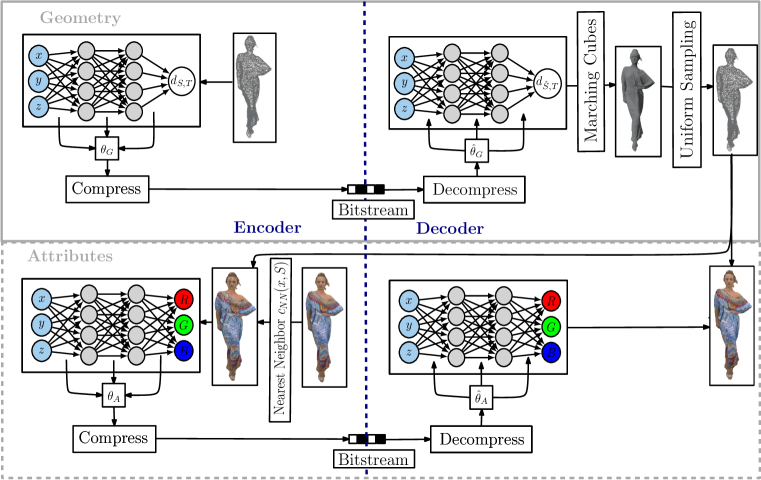
Figure 1: Overview of nf-based 3D compression. Geometry compression is in the upper part (see Sec. 3.1), while the lower part visualizes attribute compression (optional) (see Sec. 3.2). Encoding is shown on the left side. It contains two parts: a) geometry representation using nf (see Sec. 3.1) and, resp., attribute representation (see Sec. 3.2) and b) the nf parameter compression (see Sec. 3.3).

Generally, we fit a single nf to a 3D shape comprised of a pc/mesh and, optionally, another nf to the attributes (e.g. color) on the geometry. Then, we compress the parameters of the nf. Specifically, Sec. 3.1 describes how we model the geometry of 3D data - for pc as well as meshes - using truncated ndf. Further, we explain how meshes and, ultimately, pc can be recovered from df. Sec. 3.2 elaborates on additionally compressing attributes (e.g. color) of 3D data. Lastly, Sec. 3.3 describes our approach to compressing the parameters of nf representing the underlying 3D data. Fig. 1 outlines our geometry and attribute compression pipeline.

3.1 Representing Geometries with Truncated Neural Distance Fields

We represent 3D geometries implicitly using df. A df is a scalar field $\textrm{DF}:\mathbb{R}^{3}\mapsto\mathbb{R}$ that for a given 3D geometry assigns every point $x\in\mathbb{R}^{3}$ the distance $d_{S}(x)\in\mathbb{R}_{\geq 0}$ to the closest point $x_{S}\in\mathbb{R}^{3}$ on the surface $S$ of the geometry. We refer to such scalar fields as udf and omit the dependence on $x$, $d_{S}\coloneqq d_{S}(x)$. If the underlying geometry is watertight, we can further define the signed distance $d_{S}\in\mathbb{R}$ which is negative inside $S$ and positive on the outside. These instances are termed sdf. In both cases, the surface $S$ is implicitly defined by the level set $\{x|d_{S}=0\}$ of the df. In Sec. 4 we demonstrate that using udf leads to strong compression performance while being generally applicable. However, when handling watertight shapes, sdf yield further significant improvements.

Truncated Neural Distance Fields. We parameterize $d_{S}$ using nn $NF_{\theta_{G}}$ with parameters $\theta_{G}$ - in particular mlp mapping coordinates to the corresponding values of the scalar field similar to recent work on nf [33, 45, 10]. Our goal is to learn compressed representations of 3D geometries in form of the parameters $\theta_{G}$ and, thus, it is important to limit the number of parameters. To this end, we do not train ndf to parameterize the entire df $d_{S}$ but rather a truncated version of it. Hence, we intuitively only store the information in the df that is necessary to recover the 3D geometry. Such a truncated df $d_{S,T}$ is characterized by a maximal distance $d^{*}>0$ and defined as

$$d_{S,T}=\begin{cases}d_{S}&\textrm{ if }|d_{S,T}|\leq d^{*}\\ \textrm{sgn}(d_{S})d\in\{\delta\in\mathbb{R}:|\delta|>d^{*}\}&\textrm{ else.}\end{cases}$$

where $\textrm{sgn}(d_{S})$ returns the sign of $d_{S}$. We only require $|d_{S,T}|$ to be larger than $d^{*}$ but do not fix its value. Thus, the ndf can represent the 3D geometry with fewer parameters by focusing the model’s capacity on the region closest to the surface.

Architecture. We use sinusoidal activation functions in the mlp [45] combined with positional encodings [49]. This has been shown to improve the robustness of nf to quantization [46]. Chibane et al. [10] originally proposed to parameterize udf using mlp with a ReLU activation function for the output of the last layer to enforce $NF_{\theta_{G}}\geq 0$ $\forall x\in\mathbb{R}^{3}$. In contrast, we apply $\textrm{abs}(x)=\left|x\right|$ which drastically improves performance in the regime of small models (see Sec. 4.1). This originates from the fact that, unlike ReLU, $\textrm{abs}(x)$ allows to correctly represent a udf using negative values prior to the last activation function. This again increases the flexibility of the model. When modeling sdf, we apply the identity as the final activation function. More details are in the supplement.

Optimization. We train on a dataset of point-distance pairs. Following prior work [45, 10], we sample points from a mixture of three distributions - uniformly in the unit cube, uniformly from the level set and uniformly from the level set with additive Gaussian noise of standard deviation $\sigma$. This encourages learning accurate distances close to the surface. When training on pc, we restrict ourselves to approximately uniformly distributed pc. Non-uniform pc can be sub/super-sampled accordingly. In contrast to prior work on compressing other data modalities using nf [13, 46, 14, 8, 28], implicitly representing 3D geometries - in particular in the form of pc - is susceptible to overfitting as extracting a mesh from df using mc requires the level set to form a 2D manifold. A nf trained on a limited number of points may collapse to a solution where the level set rather resembles a mixture of delta peaks. We counteract overfitting using two methods. We find that $\sigma$ is an important parameter for the tradeoff between reconstruction quality and generalization (see Sec. 4.1). We find that for the distribution of natural shapes, the values $\sigma=0.01$ (sdf) and $\sigma=0.025$ (udf) work well across datasets. Secondly, we penalize the $\ell 1$-norm of $\theta$. This further has the benefit of sparsifying the parameters $\theta$ [53] and, consequently, rendering them more compressible [46]. Overall, we train nf to predict the above truncated udf/sdf using the following loss function (with $\hat{d}=NF_{\theta_{G}}(x)$):

$$\mathcal{L}_{G}(\theta_{G})=\mathcal{L}_{D}(\theta_{G})+\lambda_{\ell 1}\left|\left|\theta_{G}\right|\right|_{1}$$ (1)

where $\mathcal{L}_{D}(\theta_{G})=\textrm{E}\left[\left(\hat{d}-\textrm{sgn}(d_{S})\min(|d_{S}|,d^{*})\right)^{2}\right]$ if $|d_{S}|\leq d^{*}\text{ or }|\hat{d}|\leq d^{*}$ and 0 otherwise.

Extracting Geometries from Distance Fields. Our compressed representation implicitly encodes the 3D surface. For comparison and visualization purposes, we need to convert it to an explicit representation, namely a pc or mesh as part of our decoding step. Obtaining a uniformly sampled pc directly from a df is non-trivial. Hence, we initially convert the df into meshes in both pc compression and mesh compression scenarios. In the case of sdf, we apply mc [30] to obtain a mesh of the 3D geometry. Further, we extract meshes from udf using the recently proposed differentiable mc variant MeshUDF [21]. Note that Chibane et al. [10] originally extracted points by projecting uniform samples along the gradient direction of udf. However, this leads to undesirable clustering and holes on geometries containing varying curvature. When compressing pc, we further sample points uniformly from the extracted meshes. Notably, this is the primary reason for the inability of our compression algorithm to perform lossless compression of pc - even in the limit of very large mlp. However, it achieves state-of-the-art performance in the regime of strong compression ratios across various datasets on 3D compression - using pc/meshes with/without attributes (see Sec. 4). Further, sampling pc from the shape’s surface fundamentally limits the reconstruction quality in terms of cd. However, unlike previous methods that approximately memorize the original pc directly, our method learns the underlying geometry.

3.2 Representing 3D Attributes with Neural Fields

Besides the geometry of 3D data, we further compress its attributes (e.g. color) using nf. To this end, we follow the high level approach of other attribute compression methods and compress the attributes given the geometry [38]. Thus, after training an mlp to represent the geometry of a particular 3D shape we train a separate nf with parameters $\theta_{A}$ to correctly predict attributes on the approximated surface $\hat{S}$ of the geometry $x\in\{x|NF_{\theta_{G}}(x)=0\}$. Therefore, for a given point $x$ on $\hat{S}$ we minimize the $\ell 2$-distance to the attribute $c_{NN}(x,S)$ of the nearest neighbour on the true surface $S$:

$$\mathcal{L}_{A}(\theta_{A})=\underset{x\in\hat{S}}{\textrm{E}}\left[\left(NF_{\theta_{A}}(x)-c_{NN}(x,S)\right)^{2}\right]+\lambda_{\ell 1}\left|\left|\theta_{A}\right|\right|_{1}$$

$\lambda_{\ell 1}$ represents the strength of the regularization of $\theta_{A}$ and $c_{NN}(x,S)=c(\operatorname*{argmin}_{x^{\prime}\in S}\|x-x^{\prime}\|_{2})$ with $c(\cdot)$ extracting the attribute at a surface point. Alternatively, one may also optimize a single nf to jointly represent a geometry and its attributes. However, then the nf has to represent attributes in regions $x\notin\hat{S}$ which wastes capacity. The supplement contains an empirical verification.

3.3 Compressing Neural Fields

In the proposed compression algorithm $\theta_{G}$, and optionally $\theta_{A}$, represent the 3D data. Therefore, it is important to further compress these using nn compression techniques. We achieve this by first quantizing $\theta_{G/A}$, retraining the quantized mlp to regain the lost performance and, lastly, entropy coding the resulting quantized values. Subsequently, we describe each step in detail.

Quantization. We perform scalar quantization of $\theta_{G/A}$ using a global bitwidth $b$ which corresponds to $2^{b}$ possible values. We use a separate uniformly-spaced quantization grid for each layer of the mlp. The layer-wise step size $s_{l}$ is defined by the $\ell_{\infty}$-norm of the parameters $\theta_{G/A}^{l}$ of layer $l$ and $b$

$$s_{l}=\frac{\left|\left|\theta_{G/A}^{l}\right|\right|_{\infty}}{2^{b}-1}$$

and has to be stored to recover the quantized values. Note, that the quantization grid is centered around 0 - where $\theta_{G/A}$ peaks - to improve the gain of lossless compression using entropy coding.

Quantization-Aware Retraining. We perform a few epochs of quantization-aware retraining with a much smaller learning rate. We compute gradients during quantization-aware training using the straight-through estimator [3]. We also experimented with solely training nf using quantization-aware optimization. However, this drastically decreased convergence speed and, thus, increased the encoding time without improving performance.

Entropy Coding. Finally, we further losslessly compress the quantized parameters $\hat{\theta}_{G/A}^{l}$ using a near optimal general purpose entropy coding algorithm.

4 Experiments

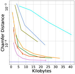
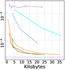
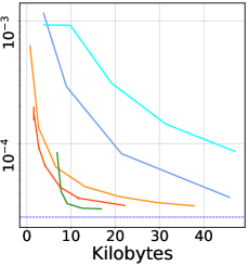
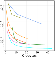
a) Watertight shapes	b) All shapes	c) MGN dataset	d) 8iVFB

Figure 2: Rate-distortion plot for pc compression on the Stanford shape repository [54] (a/b), on the MGN dataset  [4] (c) and 8iVFB [15] (d) depicting the average cd and number kilobytes for nf based on udf/sdf, pcgcv2, VQAD, Draco, GPCC and VPCC. pcgcv2/VQAD are learned neural baselines, and Draco, gpcc and vpcc are non-learned standards. On the Stanford shape repository we report performance on a subset only containing watertight shapes (a) and and all shapes (b). We do not evaluate the performance of VQAD and nf using sdf on MGN dataset since it is exclusively comprised of non-watertight shapes. There is not theo. min. in (d) as we operate directly on pc.

Sec. 4.1 depicts experiments on geometry compression - both for pc and meshes. Moreover, Sec. 4.1 analyses the impact of components our compression algorithm. Sec. 4.2 investigates the performance on 3D geometry and attributes compression. We exclusively consider color attributes.

Datasets. We conduct experiments on three datasets. Firstly, we evaluate geometry compression - pc as well as mesh compression - on a set of shapes from the Stanford shape repository [54] and a subset of the MGN dataset [4] which was also used by Chibane et al. [10]. The former are high quality meshes consisting of both watertight and non-watertight shapes. The latter are lower quality meshes of clothing. Moreover, we conduct experiments on pc extracted from 8i Voxelized Full Bodies (8iVFB) [15]. 8iVFB consists of four sequences of high quality colored pc. Each pc contains between 700,000 and 1,000,000 points. We use the first frame of each sequence in our experiments. We refer to the supplement for visualizations of each dataset.

Data Preprocessing. We center each 3D shape around the origin. Then, we scale it by dividing by the magnitude of the point (pc), resp. vertex (mesh), with largest distance to the origin. For pc, we compute the ground truth distance $d_{S}$ using the nearest neighbour in the pc. For meshes, we use a CUDA implementation to convert them to sdf [22] which we further adapt to generate udf. We train on points from a mixture of three distributions. 20% are sampled uniformly $x\sim\left[-1,1\right]^{3}$, 40% are sampled uniformly from the surface $S$ and the remaining 40% are sampled uniformly from $S$ and perturbed by additive Gaussian noise $\mathcal{N}(0;\sigma)$. For sdf we set $\sigma=0.01$ and for udf $\sigma=0.025$ if not stated otherwise. We sample 100,000 points from $S$ in our experiments on geometry compression on the Stanford shape repository and the MGN dataset and we use all points in the ground truth pc on 8iVFB. Color attributes are translated and scaled to the interval $\left[-1,1\right]$.

Evaluation and Metrics. We evaluate the reconstruction quality of geometry compression using the cd. The cd is calculated between the ground truth pc and the reconstructed pc when handling pc. For mesh compression, we report the cd between pc uniformly sampled from the ground truth and reconstructed mesh. If not stated otherwise, we use 100,000 points on the Stanford shape repository and the MGN dataset, and all available points on 8iVFB. We evaluate the quality of reconstructed attributes using a metric based on the psnr. Therefore, we compute the psnr between the attribute of each point in the ground truth pc and its nearest neighbour in the reconstructed pc, and vice versa. The final metric is then the average between both psnr. Subsequently, we simply refer to this metric as psnr. Following Strümpler et al. [46], we traverse the Rate-Distortion curve by varying the width $\in\{16,24,32,48,64,96\}$ of the mlp.

Baselines. We compare nf-based 3D compression with the non-learned baselines Draco [16], gpcc [43] and vpcc [43]. vpcc, which is based on video compression, is the non-learned state-of-the-art on compressing 3D pc including attributes. We compare our method with the learned neural baseline pcgcv2 [56] which is the state-of-the-art rdae based on 3D convolutions and VQAD [48] which builds quantized hierarchical feature grids. None of the baselines supports all data modalities/tasks used in our experiments. Geometry compression on meshes is only supported by Draco. On geometry compression using pc, we compare with all baselines. Lastly, joint geometry and attribute compression is only supported by gpcc and vpcc which we evaluate on 8iVFB. Note that Draco supports normal but not color attribute compression. When sampling from meshes, we also report the theoretical minimum, i.e. the expected distance between independently sampled point sets.

Optimization. We train all nf using a batch size of 10,000 for 500 epochs using a learning rate of $10^{-4}$ and the Adam optimizer [26]. We use $\lambda_{\ell 1}=10^{-8}$ and $d^{*}=0.1$. Each mlp contains 2 hidden layers. We follow Sitzmann et al. [45] and use the factor 30 as initialization scale. We use 16 fourier features as positional encodings on geometry compression and 8 on attribute compression. nf are quantized using a bitwidth $b=8$ and quantization-aware retraining is performed for 50 epochs using a learning rate of $10^{-7}$. Each nf is trained on a single V100 or A100.

4.1 Geometry Compression

We investigate nf-based 3D geometry compression and compare it with the baselines. We evaluate our method on pc and mesh compression and verify design choices.

Point Clouds. We evaluate pc compression on the Stanford shape repository, the MGN dataset and 8iVFB. Fig. 2 (a) & (b) depict the result on the Stanford shape repository, where we show results on the watertight subset (a) and all shapes (b), and Fig. 2 (c) & (d) contain the results on the MGN dataset and 8iVFB. Further, Fig. 3 shows qualitative results of reconstructed pc on the Stanford shape repository. We observe that for watertight shapes on the Stanford shape repository, sdf outperform the baselines for all levels of compression. On 8iVFB, nf-based compression is only outperformed by pcgcv2 whose performance drops steeply on other datasets. pcgcv2 was trained on ShapeNet [7] which contains artificial shapes with less details than the real scans in the Stanford shape repository and the MGN dataset. Despite its strong performance on 8iVFB, we hypothesize that pcgcv2 reacts very sensitive to the shift in the distribution of high frequency contents in the geometry. As expected the performance of sdf deteriorates when adding non-watertight shapes since the sdf is not well defined in this case. Further, udf also outperform the baselines stronger compression ratios. Similarly, on the MGN dataset, where we do not evaluate sdf as all shapes are non-watertight, and on 8iVFB udf perform well for strong compression ratios and are only out performed by vpcc on weaker compression ratios and by pcgcv2 on 8iVFB.

a) Draco	b) pcgcv2	c) GPCC	d) VPCC	e) VQAD	f) UDF	g) SDF	h) GT
9.2 KB	6.6 KB	4.8 KB	8.0 KB	6.9 KB	4.2 KB	4.2 KB	2.9 MB

Figure 3: We depict qualitative results on "Armadillo" of the Stanford shape repository for Draco (a), pcgcv2 (b), gpcc (c), vpcc (d), vqad (e), udf/sdf (f/g) and the ground truth (h).

Meshes. Fig. 4 (a) & (b) contains quantitative mesh compression results on the Stanford shape repository and the MGN dataset. Moreover, we refer to the supplement for qualitative results of reconstructed meshes. We only evaluate udf since both datasets contain non-watertight shapes. We find that nf-based compression outperforms Draco on more complex meshes (Stanford shape repository), while Draco can outperform udf on simpler meshes (MGN dataset). This is reasonable since the meshes in the MGN dataset contain large planar regions which benefits the edge-breaker algorithm [41] used by Draco as it is easier to represent such regions with only a few triangles.

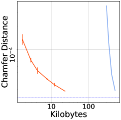
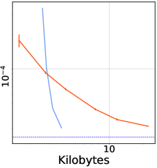
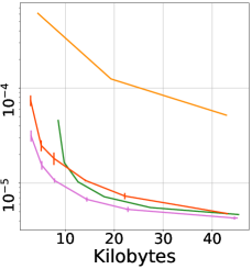
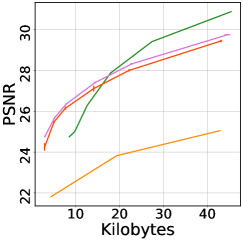
a) Stanford	b) Garments	c) Geometry	d) Color Attributes

Figure 4: Rate-distortion plot for mesh compression on the Stanford shape repository [54] (a) and the MGN dataset [4] (b), and for geometry and attribute compression (c/d) on 8iVFB [15]. On mesh compression, we report the average cd and kilobytes for nf based on udf/sdf and Draco. We do not evaluate the performance of nf using sdf due to non-watertight shapes. In (c)/(d), we report the average cd/PSNR and kilobytes for nf-based on udf/sdf, GPCC and VPCC. There is no theo. min. in (c) as we use the pc.

Table 1: We report the average encoding (top) and decoding (bottom) runtime in [s] on the Stanford shape repository of Draco, pcgcv2, GPCC, VPCC, VQAD and our approach based on udf. Draco, GPCC and VPCC are evaluated on a CPU, while nf-based compression, VQAD and PCGCv2 are evaluated on a single V100.

Draco	PCGCv2	GPCC	VPCC	VQAD	OURS
$0.06$	$0.50$	$0.26$	$46.1$	$172$	$500$
$0.04$	$0.96$	$0.04$	$2.3$	$3.3$	$1.6$

Architecture Choices. We investigate the impact of using truncated df and applying the abs activation function to the output of udf. Fig. 5 (a) depicts the result. We observe that both, truncation and abs activation function, are essential for udf with strong compression performance. Note that Chibane et al. [10] used ReLU as the final activation function. We refer to the supplement for a demonstration that ReLU performs similar to a linear activation function.

Regularization. We demonstrate the impact of regularization in Fig. 5 (b) & (c). Adding Gaussian noise $\sigma\sim\mathcal{N}(0;0.025)$ and applying an $\ell 1$-penalty to the parameters $\theta_{G}$ increasingly improves performance for larger nf. This is expected as larger nn require more regularization to prevent overfitting which is a problem for nf-based compression of 3D geometries - in contrast to other data modalities.

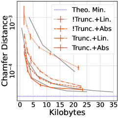
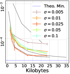
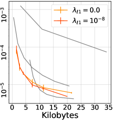
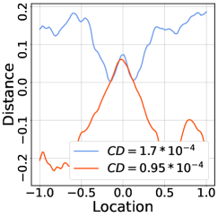
a) Truncation / Activation	b) $\sigma$	c) $\ell 1$	d) udf w/o abs

Figure 5: Impact of using truncated (Trunc.) df and the abs activation function (a), regularization effect of the standard deviation $\sigma$ added to points during training (b) on the Stanford shape repository [54]. (c) depicts the impact of the $\ell 1$ penalty on 8iVFB. We plot Draco, VPCC and GPCC in the background for reference (grey). We observe that udf demonstrate the strongest performance when combining truncated unsigned distance fields with the abs activation function (a), when adding noise of standard deviation $\sigma=0.025$ to the raw pc (b) and when applying an $\ell 1$-penalty to its parameters. We further visualize a 1D-cut through the center of the shape Armadillo of the dataset Stanford shape repository for two independently trained udf with a hidden dimension of 16 (d). We observe that the udf which converges to a sdf (red) prior to the abs activation function yields lower cd.

UDF Parameter Initialization. Interestingly, we observe that the cd of nf-based compression using udf has a large variance. In fact, the primary source of this randomness is the parameter initialization which we find by optionally fixing the random seed of the dataset and parameter initialization. For this result we refer the reader to the supplement. Moreover, qualitatively we find in Fig. 5 (d) that udf which converge to a sdf prior to the abs activation function yield lower cd.

Runtime. We compare the encoding and decoding runtime of nf-based compression with the baselines (see Tab. 1). The encoding runtime of our approach is slower compared to the baselines since it needs to fit a nn to each instance. Notably, this can be improved using meta-learned initializations [46] Interestingly, compared to vpcc, which is the only baseline that is competitive in terms of compression performance on weaker compression ratios, nf-based compression is competitive if decoding is performed on a GPU. This renders nf-based compression practical when a 3D shape needs to be decoded many more times than encoded.

4.2 Attribute Compression

Furthermore, we evaluate nf-based compression on pc containing color attributes on 8iVFB and compare it with gpcc and vpcc. Fig. 4 (c) & (d) show quantitative and Fig. 6 qualitative results. nf-based compression using sdf outperforms both baselines on geometry compression. udf outperform vpcc for strong compression ratios. On attribute compression sdf and udf outperform gpcc by a large margin, but vpcc only for stronger compression ratios. We show in the supplement that jointly compressing geometry and attributes leads to worse performance.

a) GPCC (19.3 KB)	b) VPCC (18.0 KB)	c) udf (15.7 KB)	d) sdf (15.7 KB)	e) GT (20.2 MB)

Figure 6: "Longdress" of 8iVFB for gpcc (a), vpcc (b), udf/sdf (c/d) and the target (e).

5 Discussion

We proposed an algorithm for compressing the geometry as well as attributes of 3D data using nf. We introduced two variants - one specialized to watertight shapes based on sdf and another more general approach based on udf (see Sec. 3). For watertight shapes sdf demonstrate strong geometry compression performance across all compression ratios (see Sec. 4.1). udf perform well on geometry compression - in particular for stronger compression ratios. However, vpcc can outperform udf on weaker compression ratios. Notably, the learned neural baseline pcgcv2 shows strong performance on 8iVFB, but suffers from large performance drops on Stanford shape repository and MGN dataset. This highlights another strength of nf-based neural compression - it does not exhibit the sensitivity to domain shifts of other neural compression algorithms. On attribute compression (see Sec. 4.2) sdf as well as udf outperform both baselines for stronger compression ratios, while vpcc performs better when less compression is required.

Interestingly, we observed in Sec. 4.1 that the decoding runtime of nf-based compression is competitive on a GPU. This is in line with recent findings on nf-based video compression [28]. However, the encoding runtime remains one order of magnitude larger than the next slowest method (vpcc). This gap can potentially be closed when using meta-learned initializations which have been found to improve nf-based image compression [46, 14] and speed up convergence by a factor of 10 [46].

Furthermore, we found that the performance of udf strongly depends on the parameter initialization (see Sec. 4.1). When using the abs activation function, udf are flexible regarding the values they predict prior to it. On watertight shapes, udf can converge to a function predicting the same sign inside and outside or one that predicts different signs. In presence of a sign flip, udf perform better. Thus, a promising direction for improving the more general compression method based on udf are novel initialization methods beyond the one provided in Sitzmann et al. [45]. Notably, one line of work aims at learning sdf form raw point clouds by initializing nf such that they approximately resemble an sdf of an r-ball after initialization [1, 2]. However, none of these methods work when using positional encodings which are necessary for strong performance.

References

- Atzmon and Lipman [2020] Matan Atzmon and Yaron Lipman. Sal: Sign agnostic learning of shapes from raw data. In Proceedings of the IEEE/CVF Conference on Computer Vision and Pattern Recognition, pages 2565–2574, 2020.
- Atzmon and Lipman [2021] Matan Atzmon and Yaron Lipman. Sald: Sign agnostic learning with derivatives. 9th International Conference on Learning Representations, 2021.
- Bengio et al. [2013] Yoshua Bengio, Nicholas Léonard, and Aaron Courville. Estimating or propagating gradients through stochastic neurons for conditional computation. arXiv preprint arXiv:1308.3432, 2013.
- Bhatnagar et al. [2019] Bharat Lal Bhatnagar, Garvita Tiwari, Christian Theobalt, and Gerard Pons-Moll. Multi-garment net: Learning to dress 3d people from images. In IEEE International Conference on Computer Vision (ICCV). IEEE, 2019.
- Bird et al. [2021] Thomas Bird, Johannes Ballé, Saurabh Singh, and Philip A Chou. 3d scene compression through entropy penalized neural representation functions. In 2021 Picture Coding Symposium (PCS), pages 1–5. IEEE, 2021.
- Cao et al. [2019] Chao Cao, Marius Preda, and Titus Zaharia. 3d point cloud compression: A survey. In The 24th International Conference on 3D Web Technology, pages 1–9, 2019.
- Chang et al. [2015] Angel X. Chang, Thomas Funkhouser, Leonidas Guibas, Pat Hanrahan, Qixing Huang, Zimo Li, Silvio Savarese, Manolis Savva, Shuran Song, Hao Su, Jianxiong Xiao, Li Yi, and Fisher Yu. ShapeNet: An Information-Rich 3D Model Repository. Technical Report arXiv:1512.03012 [cs.GR], Stanford University — Princeton University — Toyota Technological Institute at Chicago, 2015.
- Chen et al. [2021] Hao Chen, Bo He, Hanyu Wang, Yixuan Ren, Ser Nam Lim, and Abhinav Shrivastava. Nerv: Neural representations for videos. Advances in Neural Information Processing Systems, 34:21557–21568, 2021.
- Chen and Zhang [2019] Zhiqin Chen and Hao Zhang. Learning implicit fields for generative shape modeling. In Proceedings of the IEEE/CVF Conference on Computer Vision and Pattern Recognition, pages 5939–5948, 2019.
- Chibane et al. [2020] Julian Chibane, Gerard Pons-Moll, et al. Neural unsigned distance fields for implicit function learning. Advances in Neural Information Processing Systems, 33:21638–21652, 2020.
- Damodaran et al. [2023] Bharath Bhushan Damodaran, Muhammet Balcilar, Franck Galpin, and Pierre Hellier. Rqat-inr: Improved implicit neural image compression. arXiv preprint arXiv:2303.03028, 2023.
- De Queiroz and Chou [2016] Ricardo L De Queiroz and Philip A Chou. Compression of 3d point clouds using a region-adaptive hierarchical transform. IEEE Transactions on Image Processing, 25(8):3947–3956, 2016.
- Dupont et al. [2021] Emilien Dupont, Adam Goliński, Milad Alizadeh, Yee Whye Teh, and Arnaud Doucet. Coin: Compression with implicit neural representations. arXiv preprint arXiv:2103.03123, 2021.
- Dupont et al. [2022] Emilien Dupont, Hrushikesh Loya, Milad Alizadeh, Adam Golinski, Y Whye Teh, and Arnaud Doucet. Coin++: Neural compression across modalities. Transactions on Machine Learning Research, 2022(11), 2022.
- d’Eon et al. [2017] Eugene d’Eon, Bob Harrison, Taos Myers, and Philip A Chou. 8i voxelized full bodies-a voxelized point cloud dataset. ISO/IEC JTC1/SC29 Joint WG11/WG1 (MPEG/JPEG) input document WG11M40059/WG1M74006, 7(8):11, 2017.
- Galligan et al. [2018] Frank Galligan, Michael Hemmer, Ondrej Stava, Fan Zhang, and Jamieson Brettle. Google/draco: a library for compressing and decompressing 3d geometric meshes and point clouds, 2018.
- Gao et al. [2022] Harry Gao, Weijie Gan, Zhixin Sun, and Ulugbek S Kamilov. Sinco: A novel structural regularizer for image compression using implicit neural representations. arXiv preprint arXiv:2210.14974, 2022.
- Graphics [2017] 3D Graphics. Call for proposals for point cloud compression v2. ISO/IEC JTC1/SC29/WG11 MPEG, N 1676, 2017.
- Guarda et al. [2019] André FR Guarda, Nuno MM Rodrigues, and Fernando Pereira. Deep learning-based point cloud coding: A behavior and performance study. In 2019 8th European Workshop on Visual Information Processing (EUVIP), pages 34–39. IEEE, 2019.
- Guarda et al. [2020] André FR Guarda, Nuno MM Rodrigues, and Fernando Pereira. Deep learning-based point cloud geometry coding: Rd control through implicit and explicit quantization. In 2020 IEEE International Conference on Multimedia & Expo Workshops (ICMEW), pages 1–6. IEEE, 2020.
- Guillard et al. [2022] Benoit Guillard, Federico Stella, and Pascal Fua. Meshudf: Fast and differentiable meshing of unsigned distance field networks. In Computer Vision–ECCV 2022: 17th European Conference, Tel Aviv, Israel, October 23–27, 2022, Proceedings, Part III, pages 576–592. Springer, 2022.
- Hao et al. [2020] Zekun Hao, Hadar Averbuch-Elor, Noah Snavely, and Serge Belongie. Dualsdf: Semantic shape manipulation using a two-level representation. In Proceedings of the IEEE/CVF Conference on Computer Vision and Pattern Recognition, 2020.
- Isik [2021] Berivan Isik. Neural 3d scene compression via model compression. arXiv preprint arXiv:2105.03120, 2021.
- Isik et al. [2021] Berivan Isik, Philip Chou, Sung Jin Hwang, Nicholas Johnston, and George Toderici. Lvac: Learned volumetric attribute compression for point clouds using coordinate based networks. Frontiers in Signal Processing, page 65, 2021.
- [25] Subin Kim, Sihyun Yu, Jaeho Lee, and Jinwoo Shin. Scalable neural video representations with learnable positional features. In Advances in Neural Information Processing Systems.
- Kingma and Ba [2014] Diederik P Kingma and Jimmy Ba. Adam: A method for stochastic optimization. arXiv preprint arXiv:1412.6980, 2014.
- Ladune et al. [2022] Théo Ladune, Pierrick Philippe, Félix Henry, and Gordon Clare. Cool-chic: Coordinate-based low complexity hierarchical image codec. arXiv preprint arXiv:2212.05458, 2022.
- Lee et al. [2022] Joo Chan Lee, Daniel Rho, Jong Hwan Ko, and Eunbyung Park. Ffnerv: Flow-guided frame-wise neural representations for videos. arXiv preprint arXiv:, 2022.
- Li et al. [2023] Lingzhi Li, Zhen Shen, Zhongshu Wang, Li Shen, and Liefeng Bo. Compressing volumetric radiance fields to 1 mb. In Proceedings of the IEEE/CVF conference on computer vision and pattern recognition, 2023.
- Lorensen and Cline [1987] William E Lorensen and Harvey E Cline. Marching cubes: A high resolution 3d surface construction algorithm. ACM siggraph computer graphics, 21(4):163–169, 1987.
- Maiya et al. [2022] Shishira R Maiya, Sharath Girish, Max Ehrlich, Hanyu Wang, Kwot Sin Lee, Patrick Poirson, Pengxiang Wu, Chen Wang, and Abhinav Shrivastava. Nirvana: Neural implicit representations of videos with adaptive networks and autoregressive patch-wise modeling. arXiv preprint arXiv:2212.14593, 2022.
- Mescheder et al. [2019] Lars Mescheder, Michael Oechsle, Michael Niemeyer, Sebastian Nowozin, and Andreas Geiger. Occupancy networks: Learning 3d reconstruction in function space. In Proceedings of the IEEE/CVF conference on computer vision and pattern recognition, pages 4460–4470, 2019.
- Park et al. [2019] Jeong Joon Park, Peter Florence, Julian Straub, Richard Newcombe, and Steven Lovegrove. Deepsdf: Learning continuous signed distance functions for shape representation. In Proceedings of the IEEE/CVF conference on computer vision and pattern recognition, pages 165–174, 2019.
- Qi et al. [2017] Charles Ruizhongtai Qi, Li Yi, Hao Su, and Leonidas J Guibas. Pointnet++: Deep hierarchical feature learning on point sets in a metric space. Advances in neural information processing systems, 30, 2017.
- Quach et al. [2019] Maurice Quach, Giuseppe Valenzise, and Frederic Dufaux. Learning convolutional transforms for lossy point cloud geometry compression. In 2019 IEEE international conference on image processing (ICIP), pages 4320–4324. IEEE, 2019.
- Quach et al. [2020a] Maurice Quach, Giuseppe Valenzise, and Frederic Dufaux. Folding-based compression of point cloud attributes. In 2020 IEEE International Conference on Image Processing (ICIP), pages 3309–3313. IEEE, 2020a.
- Quach et al. [2020b] Maurice Quach, Giuseppe Valenzise, and Frederic Dufaux. Improved deep point cloud geometry compression. In 2020 IEEE 22nd International Workshop on Multimedia Signal Processing (MMSP), pages 1–6. IEEE, 2020b.
- Quach et al. [2022] Maurice Quach, Jiahao Pang, Dong Tian, Giuseppe Valenzise, and Frédéric Dufaux. Survey on deep learning-based point cloud compression. Frontiers in Signal Processing, 2022.
- Rella et al. [2022] Edoardo Mello Rella, Ajad Chhatkuli, Ender Konukoglu, and Luc Van Gool. Neural vector fields for surface representation and inference. arXiv preprint arXiv:2204.06552, 2022.
- Rho et al. [2022] Daniel Rho, Junwoo Cho, Jong Hwan Ko, and Eunbyung Park. Neural residual flow fields for efficient video representations. In Proceedings of the Asian Conference on Computer Vision, pages 3447–3463, 2022.
- Rossignac [1999] Jarek Rossignac. Edgebreaker: Connectivity compression for triangle meshes. IEEE transactions on visualization and computer graphics, 5(1):47–61, 1999.
- Schwarz and Teh [2022] Jonathan Schwarz and Yee Whye Teh. Meta-learning sparse compression networks. Transactions of Machine Learning Research, 2022.
- Schwarz et al. [2018] Sebastian Schwarz, Marius Preda, Vittorio Baroncini, Madhukar Budagavi, Pablo Cesar, Philip A Chou, Robert A Cohen, Maja Krivokuća, Sébastien Lasserre, Zhu Li, et al. Emerging mpeg standards for point cloud compression. IEEE Journal on Emerging and Selected Topics in Circuits and Systems, 9(1):133–148, 2018.
- Sheng et al. [2021] Xihua Sheng, Li Li, Dong Liu, Zhiwei Xiong, Zhu Li, and Feng Wu. Deep-pcac: An end-to-end deep lossy compression framework for point cloud attributes. IEEE Transactions on Multimedia, 24:2617–2632, 2021.
- Sitzmann et al. [2020] Vincent Sitzmann, Julien Martel, Alexander Bergman, David Lindell, and Gordon Wetzstein. Implicit neural representations with periodic activation functions. Advances in Neural Information Processing Systems, 33:7462–7473, 2020.
- Strümpler et al. [2022] Yannick Strümpler, Janis Postels, Ren Yang, Luc Van Gool, and Federico Tombari. Implicit neural representations for image compression. In Computer Vision–ECCV 2022: 17th European Conference, Tel Aviv, Israel, October 23–27, 2022, Proceedings, Part XXVI, pages 74–91. Springer, 2022.
- Takikawa et al. [2021] Towaki Takikawa, Joey Litalien, Kangxue Yin, Karsten Kreis, Charles Loop, Derek Nowrouzezahrai, Alec Jacobson, Morgan McGuire, and Sanja Fidler. Neural geometric level of detail: Real-time rendering with implicit 3d shapes. In Proceedings of the IEEE/CVF Conference on Computer Vision and Pattern Recognition, pages 11358–11367, 2021.
- Takikawa et al. [2022] Towaki Takikawa, Alex Evans, Jonathan Tremblay, Thomas Müller, Morgan McGuire, Alec Jacobson, and Sanja Fidler. Variable bitrate neural fields. In ACM SIGGRAPH 2022 Conference Proceedings, pages 1–9, 2022.
- Tancik et al. [2020] Matthew Tancik, Pratul Srinivasan, Ben Mildenhall, Sara Fridovich-Keil, Nithin Raghavan, Utkarsh Singhal, Ravi Ramamoorthi, Jonathan Barron, and Ren Ng. Fourier features let networks learn high frequency functions in low dimensional domains. Advances in Neural Information Processing Systems, 33:7537–7547, 2020.
- Tancik et al. [2021] Matthew Tancik, Ben Mildenhall, Terrance Wang, Divi Schmidt, Pratul P Srinivasan, Jonathan T Barron, and Ren Ng. Learned initializations for optimizing coordinate-based neural representations. In Proceedings of the IEEE/CVF Conference on Computer Vision and Pattern Recognition, pages 2846–2855, 2021.
- Tang et al. [2018] Danhang Tang, Mingsong Dou, Peter Lincoln, Philip Davidson, Kaiwen Guo, Jonathan Taylor, Sean Fanello, Cem Keskin, Adarsh Kowdle, Sofien Bouaziz, et al. Real-time compression and streaming of 4d performances. ACM Transactions on Graphics (TOG), 37(6):1–11, 2018.
- Tang et al. [2020] Danhang Tang, Saurabh Singh, Philip A Chou, Christian Hane, Mingsong Dou, Sean Fanello, Jonathan Taylor, Philip Davidson, Onur G Guleryuz, Yinda Zhang, et al. Deep implicit volume compression. In Proceedings of the IEEE/CVF conference on computer vision and pattern recognition, pages 1293–1303, 2020.
- Tibshirani [1996] Robert Tibshirani. Regression shrinkage and selection via the lasso. Journal of the Royal Statistical Society: Series B (Methodological), 58(1):267–288, 1996.
- Turk and Levoy [1994] Greg Turk and Marc Levoy. Zippered polygon meshes from range images. In Proceedings of the 21st annual conference on Computer graphics and interactive techniques, pages 311–318, 1994.
- Wang and Ma [2022] Jianqiang Wang and Zhan Ma. Sparse tensor-based point cloud attribute compression. In 2022 IEEE 5th International Conference on Multimedia Information Processing and Retrieval (MIPR), pages 59–64. IEEE, 2022.
- Wang et al. [2021a] Jianqiang Wang, Dandan Ding, Zhu Li, and Zhan Ma. Multiscale point cloud geometry compression. In 2021 Data Compression Conference (DCC), pages 73–82. IEEE, 2021a.
- Wang et al. [2021b] Jianqiang Wang, Hao Zhu, Haojie Liu, and Zhan Ma. Lossy point cloud geometry compression via end-to-end learning. IEEE Transactions on Circuits and Systems for Video Technology, 31(12):4909–4923, 2021b.
- Xie et al. [2022] Yiheng Xie, Towaki Takikawa, Shunsuke Saito, Or Litany, Shiqin Yan, Numair Khan, Federico Tombari, James Tompkin, Vincent Sitzmann, and Srinath Sridhar. Neural fields in visual computing and beyond. Computer Graphics Forum, 2022.
- Zhang et al. [2021] Yunfan Zhang, Ties van Rozendaal, Johann Brehmer, Markus Nagel, and Taco Cohen. Implicit neural video compression. In ICLR Workshop on Deep Generative Models for Highly Structured Data, 2021.