An improved method to measure $\rm{}^{12}C/^{13}C$ and $\rm{}^{14}N/^{15}N$ abundance ratios: revisiting CN isotopologues in the Galactic outer disk

Abstract

The variations of elemental abundance and their ratios along the Galactocentric radius result from the chemical evolution of the Milky Way disks. The $\rm{}^{12}C/^{13}C$ ratio in particular is often used as a proxy to determine other isotopic ratios, such as $\rm{}^{16}O/^{18}O$ and $\rm{}^{14}N/^{15}N$. Measurements of $\rm{}^{12}CN$ and $\rm{}^{13}CN$ (or $\rm C^{15}N$) – with their optical depths corrected via their hyper-fine structure lines – have traditionally been exploited to constrain the Galactocentric gradients of the CNO isotopic ratios. Such methods typically make several simplifying assumptions (e.g. a filling factor of unity, the Rayleigh–Jeans approximation, and the neglect of the cosmic microwave background) while adopting a single average gas phase. However, these simplifications introduce significant biases to the measured $\rm{}^{12}C/^{13}C$ and $\rm{}^{14}N/^{15}N$. We demonstrate that exploiting the optically thin satellite lines of ¹²CN constitutes a more reliable new method to derive $\rm{}^{12}C/^{13}C$ and $\rm{}^{14}N/^{15}N$ from CN isotopologues. We apply this satellite-line method to new IRAM 30-m observations of ¹²CN, ¹³CN, and C¹⁵N $N=1\to 0$ towards 15 metal-poor molecular clouds in the Galactic outer disk ($R_{\rm gc}>$ 12 kpc), supplemented by data from the literature. After updating their Galactocentric distances, we find that $\rm{}^{12}C/^{13}C$ and $\rm{}^{14}N/^{15}N$ gradients are in good agreement with those derived using independent optically thin molecular tracers, even in regions with the lowest metallicities. We therefore recommend using optically thin tracers for Galactic and extragalactic CNO isotopic measurements, which avoids the biases associated with the traditional method.

1 Introduction

The isotopic abundance ratios of carbon, nitrogen, and oxygen, namely $\rm{}^{12}C/^{13}C$ ($R_{\rm{}^{12}C/^{13}C}$), $\rm{}^{16}O/^{18}O$ ($R_{\rm{}^{16}O/^{18}O}$), and $\rm{}^{14}N/^{15}N$ ($R_{\rm{}^{14}N/^{15}N}$), are crucial for constraining the evolutionary chemical history of the Milky Way(Wilson & Rood, 1994; Romano, 2022). Systematic variations in these ratios are caused by the different time scales according to which different isotopes are ejected in the interstellar medium by stars of different initial masses (Nomoto et al., 2013; Karakas & Lattanzio, 2014; Cristallo et al., 2015; Limongi & Chieffi, 2018). Furthermore, the growth history of the Galactic thin disk has a significant impact on these ratios, resulting in strong evolutionary features (e.g., Matteucci & D’Antona, 1991; Henkel & Mauersberger, 1993; Romano & Matteucci, 2003; Romano et al., 2017, 2019). In particular, $R_{\rm{}^{12}C/^{13}C}$, $R_{\rm{}^{16}O/^{18}O}$, and $R_{\rm{}^{14}N/^{15}N}$ generally increase with Galactocentric distances ($R_{\rm gc}$) (e.g., Wilson & Rood, 1994; Wouterloot et al., 2008; Jacob et al., 2020; Zhang et al., 2020; Chen et al., 2021), though $R_{\rm{}^{14}N/^{15}N}$ shows a decreasing trend in the Galactic outer disk(Colzi et al., 2022).

The production of metal elements and their isotopes depends on nucleosynthesis and stellar evolutionary processes  (Burbidge et al., 1957; Meyer, 1994). For example, the $\rm{}^{12}C$ production is dominated by triple-$\alpha$ reactions (Timmes et al., 1995; Woosley & Weaver, 1995), while $\rm{}^{13}C$ can be produced by the CNO-I cycle, $\rm{}^{12}C$-burning, or proton-capture nucleosynthesis (Meynet & Maeder, 2002b; Botelho et al., 2020). The $\rm{}^{14}N$ can be synthesized through the cold CNO cycle in the H-burning zone of stars (Karakas & Lattanzio, 2014; Romano, 2022), $\rm{}^{12}C$-burning in the low-metallicity fast massive rotators, and proton-capture reactions in the hot convective envelope of intermediate-mass stars (Marigo, 2001; Pettini et al., 2002; Meynet & Maeder, 2002a; Limongi & Chieffi, 2018; Botelho et al., 2020). The production of $\rm{}^{15}N$ and $\rm{}^{13}C$ can happen in hot-CNO cycles in H-rich material accreting on white dwarfs (Audouze et al., 1973; Wiescher et al., 2010; Romano, 2022). The Galactic $\rm{}^{15}N$ is contributed by novae (Romano et al., 2017) and proton ingestion in the He shell of massive stars (Pignatari et al., 2015).

Despite extensive study, the isotopic ratio gradients in the low-metallicity outer disk of the Milky Way remain poorly constrained. To date, measurements of only one target, WB89-391, at a Galactocentric distance $R_{\rm gc}$ $\gtrsim$ 12 kpc, have been made for the $R_{\rm{}^{12}C/^{13}C}$ ratio using CN isotopologues (Milam et al., 2005). This single measurement ($R_{\rm{}^{12}C/^{13}C}$ $\sim$ 134) critically constrains the $R_{\rm{}^{14}N/^{15}N}$ and $R_{\rm{}^{16}O/^{18}O}$ gradients derived from C-bearing isotopologues. To fully constrain all CNO isotopic ratios in the outer Galactic disk, more data and more precise measurements of $R_{\rm{}^{12}C/^{13}C}$ are needed.

The $R_{\rm{}^{12}C/^{13}C}$ ratios in the ISM are determined using pairs of molecular isotopologues. Measurements of $\rm{}^{12}C^{18}O/^{13}C^{18}O$ (e.g., Langer & Penzias, 1990; Wouterloot & Brand, 1996; Giannetti et al., 2014) or $\rm{}^{12}C^{34}S/^{13}C^{34}S$ (Yan et al., 2023) may be limited to nearby strong targets because of the weak emission of $\rm{}^{13}C^{18}O$ or $\rm{}^{13}C^{34}S$ expected in the metal-poor outer disk clouds. Molecules such as $\rm H_{2}CO/H_{2}^{13}CO$ (Henkel et al., 1982, 1985; Yan et al., 2019), $\rm CH^{+}/^{13}CH^{+}$ (Ritchey et al., 2011), and $\rm CH/^{13}CH$ (Jacob et al., 2020) can be good tracers to derive $R_{\rm{}^{12}C/^{13}C}$ through their absorption lines. $\rm H_{2}CO$ isotopologues can be absorbed by the CMB but their absorption lines are still weak because of low abundance. The CH and $\rm CH^{+}$ absorption lines are in rare cases of strong background continuum and/or high column density. The optically-thick line pairs, such as ¹³CN and ¹²CN  $N=1\to 0$, which require corrections to their optical depths that are mostly determined by fitting hyper-fine-structure (HfS) lines (Savage et al., 2002; Milam et al., 2005), could be adopted to measure $R_{\rm{}^{12}C/^{13}C}$ in the outer disk regions. This method can also derive $R_{\rm{}^{14}N/^{15}N}$ without any assumptions of $R_{\rm{}^{12}C/^{13}C}$ (Adande & Ziurys, 2012).

The current commonly used method for deriving the $R_{\rm{}^{12}C/^{13}C}$ from CN isotopologues, with the HfS fitting, makes several assumptions and approximations. In order to derive the column density (i.e., Mangum & Shirley, 2015), it assumes identical excitation temperature of ¹²CN and ¹³CN. However differential radiative trapping among spectral lines, due to different optical depths (if these are significant), can yield different excitation temperatures between the spectral lines. Also, a single gas phase is typically used (necessitated by the small number of transitions per species typically available, and lack of standard molecular cloud models), while a range of excitation conditions is present in molecular clouds impacting the volume-average excitation temperatures of the CN isotopologues. In addition, most studies (e.g., Savage et al., 2002; Milam et al., 2005) adopt the Rayleigh-Jeans (R-J) approximation, which becomes increasingly poor when $h\nu_{\rm ik}/k_{\rm B}T_{\rm ex}\lesssim 1$ starts approaching unity (and is of course inappropriate when $h\nu_{\rm ik}/k_{\rm B}T_{\rm ex}\gtrsim 1$). In the cold ($T_{\rm kin}\sim 15-20$ K), often sub-thermal line excitation conditions ($T_{\rm ex}$$<$$T_{\rm kin}$) prevailing in the bulk of molecular clouds in the quiescent ISM of the Galaxy, the R-J approximation is simply not good enough for abundance ratio studies conducted using the CN $N=1\to 0$ and $N=2\to 1$ at 112 GHz and 224 GHz. In addition, the cosmic microwave background (CMB) must be taken into account given that for the low-temperature molecular clouds where such isotopologue studies are conducted (and with the possible sub-thermal excitation of the lines utilized) , the line Planck temperature $J(\nu_{\rm ik},T_{\rm ex})=h\nu_{\rm ik}/k_{\rm B}\,\left(e^{h\nu_{\rm ik}/k_{B}T_{\rm ex}}-1\right)^{-1}$ can be so low that the $J(\nu_{\rm ik},T_{\rm CMB})$ is no longer negligible for the frequencies used, even for the low $T_{\rm CMB,0}=2.72$ K) in the local Universe (see Zhang et al., 2016, for even more serious effects in the high-z Universe where $T_{\rm CMB}(z)=(1+z)T_{\rm CMB,0}$). All these assumptions/approximations have been used for such studies conducted in widely different ISM environments, ranging from the very cold and quiescent ISM in the Galactic outer disk (Milam et al., 2005), where they become questionable, up to the warm, dense ISM in starburst galaxies (e.g., Henkel et al., 1993; Henkel et al., 2014; Tang et al., 2019) where the aforementioned assumptions/approximations should be adequate.

In this work, we introduce an improved method to derive $\rm{}^{12}C/^{13}C$ from CN isotopologues and compare it with current methods. We list the basic assumptions of the current methods of using CN isotopologues to derive $R_{\rm{}^{12}C/^{13}C}$ and $R_{\rm{}^{14}N/^{15}N}$. We also present new ¹²CN, ¹³CN and C¹⁵N $N=1\to 0$ observations in a small sample of molecular clouds with $R_{\rm gc}$ $>$ 12 kpc, which allows new constraints on the $R_{\rm{}^{12}C/^{13}C}$ and $R_{\rm{}^{14}N/^{15}N}$ outer gradients. Section 2 presents the observations and the data reduction. In Section 3, we list the current methods of deriving $R_{\rm{}^{12}C/^{13}C}$ and $R_{\rm{}^{14}N/^{15}N}$ with CN isotopologues and show their underlying assumptions and drawbacks. In Section 4, we introduce a new method to derive $R_{\rm{}^{12}C/^{13}C}$ and $R_{\rm{}^{14}N/^{15}N}$. In Section 5, we present newly measured isotopic ratios and data derived from the improved traditional methods and the new method. In Section 6, we compare the Galactic $R_{\rm{}^{12}C/^{13}C}$ and $R_{\rm{}^{14}N/^{15}N}$ obtained by the different methods. We also compare CN isotopologues and the optically thin tracers $\rm{}^{12}C^{18}O/^{13}C^{18}O$, and we discuss physical and chemical processes that may bias the abundances. We present the main conclusion in Section 7.

2 Observations and data reduction

2.1 Sample Selection

We select 15 molecular clouds from the literature (Savage et al., 2002; Milam et al., 2005; Wouterloot et al., 2008; Sun et al., 2015; Li et al., 2016; Sun et al., 2017; Reid et al., 2019) based on the following criteria: (a). located in the Galactic radii range of (11 – 22) kpc; and (b). with strong $\rm{}^{13}CO$ $J=1\to 0$ detections of $\geq 5$K (in $T_{\rm mb}$) in Sun et al. (2015, 2017). This allows a good chance of detecting CN isotopologues because of an expected strong ¹²CN $N=1\to 0$ emission. We also include WB89 391 from Milam et al. (2005), which provided the only $R_{\rm{}^{12}C/^{13}C}$ data at $R_{\rm gc}>12$ kpc from CN isotopologues before our study.

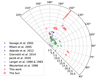
Figure 1: Spatial distribution of sources in the Galactic plane. The pole is the Galactic center, and the red star shows the position of the Sun (Reid et al., 2019). Rings indicate the Galactocentric distances ($R_{\rm gc}$). Red squares show our new observations. Black circles, blue multiplication signs, purple multiplication signs, green triangles, magenta thin diamonds, steel-blue rectangles, purple plus signs, and red diamonds, are positions of sources from Savage et al. (2002), Milam et al. (2005), Adande & Ziurys (2012), Giannetti et al. (2014), Jacob et al. (2020), Langer & Penzias (1990, 1993), and Wouterloot & Brand (1996), respectively.

2.1.1 Revision of distances

We update the Galactocentric distances, for both our targets and sources in the literature(Savage et al., 2002; Milam et al., 2005; Adande & Ziurys, 2012; Giannetti et al., 2014; Jacob et al., 2020; Langer & Penzias, 1990, 1993; Wouterloot & Brand, 1996). For sources with direct trigonometric measurements (Reid et al., 2014, 2019), we adopt the measured values. For the others, we apply the up-to-date Galactic rotation curve model (Reid et al., 2019), which has been well calibrated with accurate trigonometric measurements, to obtain the kinematic distance. Specifically, we employed results based on the Parallax-Based Distance Calculator (Reid et al., 2016) . The Galactocentric distances are then derived with the following equation:

$$R_{\rm gc}=\sqrt{R_{\odot}^{2}+R_{\rm h}^{2}-2R_{\odot}R_{\rm h}{\rm cos}l},$$ (1)

where $R_{\odot}=8.15\ \rm kpc$ is the distance of the Sun from the centre of the Milky Way (Reid et al., 2019), $R_{\rm h}$ is the heliocentric distance, $R_{\rm gc}$ is the Galactocentric distance, and $l$ is the Galactic longitude of the sources.

Figure 1 shows the locations of these sources. The Probability density functions (PDFs) generated by the distance calculator are presented in Appendix A. In Table 1 we list the coordinates, velocity at the frame of Local Standard of Rest (LSR) ($V_{\rm LSR}$), estimated heliocentric distances, updated $R_{\rm gc}$, and observing time.

2.2 IRAM 30-m observations

Fourteen targets were observed with the 30-m telescope in Project 031-17 (PI: Zhi-Yu Zhang) from August 31 to September 05, 2017. An additional target, G211.59, was observed as part of Project 005-20 (PI: Junzhi Wang) during August 5–9, 2020. To ensure data quality, we only used observations with a precipitable water vapor (PWV) $<$ 10 mm and discarded data with PWV $\gtrsim$ 10 mm. In Project 031-17, the typical system temperature ($T_{\rm sys}$) was $\sim\rm(100-200)\,K$ and $\sim\rm(200-400)\,K$ at 3-mm and 2-mm bands, respectively. For G211.59, $T_{\rm sys}$ was $\sim\rm(150-200)\,K$ and $\sim\rm(400-650)\,K$ at 3-mm and 2-mm bands, respectively.

Both projects utilized the Eight Mixer Receiver (EMIR) as the front end, with both E090 and E150 receivers under similar frequency setups. The backend is the Fast Fourier Transform Spectrometers working at 200 kHz resolution (FTS200), corresponding to $\sim 0.53\ \rm km\cdot s^{-1}$ and $\sim 0.34\ \rm km\cdot s^{-1}$ at 3-mm and 2-mm, respectively. The frequency setup covers ${}^{13}\rm{CO}$ $J=1\to 0$ ($\nu_{\rm rest}=$ 110.201 GHz), $\rm{}^{12}CN$ $N=1\to 0$ ($\nu_{\rm rest}=$ 113.490 GHz), $\rm{}^{13}CN$ $N=1\to 0$ ($\nu_{\rm rest}=$ 108.780 GHz), and $\rm C^{15}N$ $N=1\to 0$ ($\nu_{\rm rest}=$ 110.024 GHz). In addition, our setup at 2-mm covers the $\rm H^{13}CN$ $J=2\to 1$ ($\nu_{\rm rest}=$ 172.678 GHz) and $\rm HC^{15}N$ $J=2\to 1$ ($\nu_{\rm rest}=$ 172.108 GHz).

Planets, i.e., Saturn, Mars, and Venus, were used to perform the focus calibration, each after a prior pointing correction. In a few cases, we adopted PKS 2251+158, PKS 0316+413 and W3(OH) for the focus, when the planets were not available. These focus corrections were performed at the beginning of each observing slot and were repeated within 30 minutes after sunset or sunrise. We perform regular pointing calibration every 1–2 hours, with strong point continuum sources within the 15$\degr$ radius of targets, e.g., PKS 1749+096, PKS 0736+017, PKS 0316+413, NGC7538, and W3(OH). The typical pointing error is $\sim$ 3^′′ (rms).

The observations were performed in two steps: we first performed an On-The-Fly (OTF) mapping towards each target, to get the spatial distribution of $\rm{}^{13}CO$ $J=1\to 0$ emission. Then we performed a single-pointing deep integration towards the emission peak position on the $\rm{}^{13}CO$ $J=1\to 0$ map. During the OTF mapping, we scanned along both right ascension (R.A.) and declination (Dec.) directions, with a spatial scan interval of 9.0^′′. Along the direction of each scan, it outputs a spectrum every 0.5 sec, which makes a 4.8 ^′′ interval along the scan direction. Each OTF map covers an area of $\sim 2.4^{\prime}\times 2.4^{\prime}$.

We adopted a positional beam-switch mode and performed deep integration at the peak position of $\rm{}^{13}CO$ $J=1\to 0$ for the extended targets. The OFF positions were set 10^′ (in Azimuth) away from the target. For targets with compact $\rm{}^{13}CO$ $J=1\to 0$ emission (spatial FWHM $<1^{\prime}$), we use the wobbler switch mode. The beam switching used had a frequency of 2 Hz and a throw of 120^′′ (in Azimuth) on either side of the target (to correct for any first-order beam-asymmetric beam effects between the two throw positions).

The beam sizes of the IRAM 30-m telescope are $\sim$ 22^′′ and 14^′′ at 110 GHz ($\rm{}^{13}CO$) and 170 GHz ($\rm H^{13}CN$), with main beam efficiencies ($\eta_{\rm mb}$) of $\sim 0.78$ and $\sim 0.69$, respectively. We present the integration time of each target in Table 1. The noise levels of the final spectra are listed in Table 2. Particularly, we list the transitions of CN isotopologues and the main beam efficiencies ($\eta_{\rm mb}$) of IRAM 30-m at the frequency of each transition in Table 3.

Table 1: Target information.

Sources	$l$	$b$	$V_{\rm{LSR}}$	$R_{\rm{h}}$	$R_{\rm{gc}}$	$t_{\rm obs}$	references
	(degree)	(degree)	($\rm km\cdot s^{-1}$)	(kpc)	(kpc)	(hours)
G211.59	211.593	1.056	45.0	$4.18\ \pm 0.18$	$11.92^{*}\ \pm 0.22$	9.72	Reid et al. (2019)
G37.350	37.350	1.050	$-$53.9	$17.87\ \pm 0.49$	$12.42\ \pm 0.46$	1.20	Sun et al. (2017)
G44.8	44.800	0.658	$-$62.1	$17.43\ \pm 1.10$	$12.98\ \pm 0.99$	1.30	Sun et al. (2017)
IRAS0245	136.357	0.958	$-$61.4	$5.25\ \pm 0.57$	$12.49\ \pm 0.53$	3.15	Li et al. (2016)
SUN15 14N	109.292	2.083	$-$101.1	$10.67\ \pm 0.70$	$15.41\ \pm 0.62$	0.55	Sun et al. (2015)
SUN15 18	109.792	2.717	$-$99.3	$10.58\ \pm 0.71$	$15.38\ \pm 0.63$	0.84	Sun et al. (2015)
SUN15 21	114.342	0.783	$-$100.9	$10.25\ \pm 0.71$	$15.50\ \pm 0.63$	0.73	Sun et al. (2015)
SUN15 34	122.775	2.525	$-$100.7	$10.24\ \pm 0.62$	$16.17\ \pm 0.58$	0.55	Sun et al. (2015)
SUN15 56	137.758	$-$0.983	$-$103.6	$17.53\ \pm 3.61$	$24.19\ \pm 3.52$	1.63	Sun et al. (2015)
SUN15 57	137.775	$-$1.067	$-$102.1	$16.72\ \pm 3.47$	$23.40\ \pm 3.38$	0.94	Sun et al. (2015)
SUN15 7W	104.983	3.317	$-$102.7	$10.98\ \pm 0.62$	$15.26\ \pm 0.54$	0.77	Sun et al. (2015)
WB89 380	124.644	2.540	$-$86.2	$5.53\ \pm 0.51$	$12.17\ \pm 0.45$	6.08	Wouterloot et al. (2008)
WB89 391	125.802	3.048	$-$86.0	$5.45\ \pm 0.50$	$12.16\ \pm 0.44$	4.38	Wouterloot et al. (2008)
WB89 437	135.277	2.800	$-$71.6	$5.65\ \pm 0.39$	$13.10^{*}\ \pm 0.38$	5.67	Wouterloot et al. (2008)
WB89 501	145.199	2.987	$-$58.1	$4.87\ \pm 0.51$	$12.46\ \pm 0.49$	2.07	Wouterloot et al. (2008)

• Column 1: source names. Columns 2 and 3: the Galactic coordinates of sources. Column 4: $V_{\rm{LSR}}$ values gained by fitting a gauss profile for ¹³CO line at $J=1\to 0$ at 110201.354 MHz. Column 5: Heliocentric distances. Column 6: Galactocentric distances. Column 7: single-pointing observing time. Column 8: source references. *: The distance of G211.59 and WB89 437 are directly measured by $\rm H_{2}O$ masers in Reid et al. (2014, 2019).

2.3 Data reduction

For data reduction, we used the Continuum and Line Analysis Single-dish Software (CLASS) package from the Grenoble Image and Line Data Analysis Software (GILDAS, Guilloteau & Lucas, 2000). For each sideband, three independent Fast Fourier Transform Spectroscopy (FTS) units cover a 4-GHz bandwidth, which sometimes causes different continuum levels on the same spectrum (so-called the platforming effect). Therefore, we first split each spectrum into three frequency ranges (corresponding to the three units) and treat them independently. Then we locate the line-free channels and subtract a first-order baseline for each spectrum with command BASE. For spectra affected by apparent standing waves, which are less than 5% of the total, a sinusoidal function is adopted to fit and subtract the baseline.

We discarded spectra with high noise levels: $\sigma_{\rm obs}$$>$$1.2\sigma_{\rm theoretical}$. Spectra at the same position are then averaged with the default weighting setup of TIME, by which the weight is proportional to the integrated time, frequency, and $T_{\rm sys}^{-2}$. In Table 2, we list the typical root-mean-square (RMS) of the antenna temperature in the $T^{\star}_{\rm A}$ scale at 3-mm. For the IRAM 30-m telescope, the antenna temperature scale denotes one corrected only for atmospheric absorption.

Table 2: The RMS of 3-mm spectra in our targets.

Sources	E0UI			E0UO
	Frequency Range	Channel Width	RMS	Frequency Range	Channel Width	RMS
	(GHz)	($\rm km\cdot s^{-1}$)	(mK)	(GHz)	($\rm km\cdot s^{-1}$)	(mK)
G211.59	$103.318-105.826$	$0.553-0.567$	3.0	$109.557-113.608$	$0.515-0.534$	4.1
G37.350	$106.850-110.900$	$0.528-0.548$	7.9	$110.580-114.629$	$0.511-0.529$	13
G44.8	$106.850-110.900$	$0.528-0.548$	8.1	$110.580-114.629$	$0.511-0.529$	13
IRAS0245	$106.850-110.914$	$0.528-0.548$	4.8	$110.580-114.643$	$0.511-0.529$	7.3
SUN15 14N	$106.850-110.900$	$0.528-0.548$	12	$110.580-114.629$	$0.511-0.529$	19
SUN15 18	$106.850-110.900$	$0.528-0.548$	17	$110.580-114.629$	$0.511-0.529$	19
SUN15 21	$106.851-110.899$	$0.528-0.548$	10	$110.579-114.628$	$0.511-0.529$	16
SUN15 34	$106.851-110.900$	$0.528-0.548$	12	$110.579-114.628$	$0.511-0.529$	20
SUN15 56	$106.851-110.899$	$0.528-0.548$	6.0	$110.579-114.628$	$0.511-0.529$	9.4
SUN15 57	$106.851-110.900$	$0.528-0.548$	7.6	$110.579-114.628$	$0.511-0.529$	12
SUN15 7W	$106.851-110.899$	$0.528-0.548$	14	$110.579-114.628$	$0.511-0.529$	23
WB89 380	$106.851-110.899$	$0.528-0.548$	3.5	$110.580-114.629$	$0.511-0.529$	5.0
WB89 391	$106.851-110.900$	$0.528-0.548$	4.0	$110.579-114.628$	$0.511-0.529$	6.2
WB89 437	$106.851-110.900$	$0.528-0.548$	3.5	$110.579-114.628$	$0.511-0.529$	4.9
WB89 501	$106.851-110.900$	$0.528-0.548$	5.6	$110.579-114.629$	$0.511-0.529$	8.6

Table 3: Transitions of CN isotopologues and IRAM 30-m main beam efficiencies.

Isotopologue Transitions		Componentsa	Frequency	Relative intensityb	$\eta_{\rm mb}=B_{\rm eff}/F_{\rm eff}$
			(MHz)
	$J=1/2\to 1/2$	$F=1/2\to 1/2$	113123.369	0.012	0.7819
		$F=1/2\to 3/2$	113144.190	0.099	0.7819
		$F=3/2\to 1/2$	113170.535	0.096	0.7819
$\rm{}^{12}CN$		$F=3/2\to 3/2$	113191.325	0.125	0.7819
$N=1\to 0$	$J=3/2\to 1/2$	$F=3/2\to 1/2$	113488.142	0.126	0.7816
		$F=5/2\to 3/2$	113490.985	0.334	0.7816
		$F=1/2\to 1/2$	113499.643	0.099	0.7816
		$F=3/2\to 3/2$	113508.934	0.097	0.7815
		$F=1/2\to 3/2$	113520.422	0.012	0.7815
$\rm{}^{13}CN$	$J=3/2\to 1/2$	$F=3\to 2$	108780.201	0.195	0.7864
$N=1\to 0$	$F_{13}=2\to 1$	$F=2\to 1$	108782.374	0.103	0.7864
$\rm C^{15}N$	$J=3/2\to 1/2$	$F=1\to 0$	110023.540	0.165	0.7851
$N=1\to 0$		$F=2\to 1$	110024.590	0.417	0.7851

• a. For $\rm{}^{13}CN$ and $\rm C^{15}N$ $N=1\to 0$, we only list the two strongest components considered in our intensity estimation.
  b. The intrinsic ratio between the intensity of individual line components and the total intensity of all the line components (based on CDMS/JPL).

2.3.1 Line intensities

We adopt the rest frequencies of molecular lines from NASA’s Jet Propulsion Laboratory (JPL). We first fit a Gaussian profile to the ${}^{13}\rm{CO}$ $J=1\to 0$ spectra, which are all single peaked. Then, we use $\Delta v$= $8\times$ FWHM/$\rm{2\sqrt{2ln2}}$ as the velocity range for other emission lines, by assuming that all lines of the same target have the same line width. The line-free channels are adopted as $\sim 4\times\Delta v$ at both sides of each line. Then we obtain the velocity-integrated-intensity in the velocity range of $\Delta v$, using the following equation:

$$I_{\rm line}=\int_{\Delta v}T_{\rm mb}dv,$$ (2)

where $\Delta v$ is the Full Width at Zero Intensity (FWZI) of the emission line, which is set to be $8\times$ FWHM/$\rm 2\sqrt{2ln2}$. $T_{\rm mb}(=F_{\rm eff}/B_{\rm eff}\cdot T_{\rm A}^{\star}=T_{\rm A}^{\star}/\eta_{\rm mb})$ is the main beam temperature; and $T_{\rm A}^{\star}$, $F_{\rm eff}$, and $B_{\rm eff}$ are the antenna temperature, the forward efficiency, and the telescope beam efficiency, respectively.

We derive the thermal noise error following Greve et al. (2009), with Eq. 3, which accounts for both the one associated with the velocity-integral of the line intensity over its FWZI and the one associated with the subtracted baseline level (the latter becoming significant only if a wide line leaves little baseline “room” within a spectral window).

$$\sigma_{I_{\rm line}}=\sigma_{T_{\rm{mb,chan}}}\Delta v_{\rm{res}}\sqrt{N_{\rm{line}}(1+\frac{N_{\rm{line}}}{N_{\rm{base}}})},$$ (3)

where $\sigma_{T_{\rm mb,chan}}$ is the channel noise level of the main beam temperature, $N_{\rm line}$ is the number of channels covering the FWZI of the line, $N_{\rm{base}}$ is the number of line-free channels as the baseline, and $\Delta v_{\rm{res}}$ is the velocity resolution of the spectrum. The flux calibration and beam efficiency uncertainties (typically $\sim$ 10–15% in such single-dish measurements), are not included in our final line ratio uncertainties since all lines were measured simultaneously in our observations (the flux calibration and main beam efficiency factors are applied multiplicatively).

The two strongest satellite lines of $\rm{}^{13}CN$ $N=1\to 0$ ($\nu_{\rm rest}$ at 108.780 and 108.782 GHz) are blended, with a velocity separation of $\sim 6.0\ \rm kms^{-1}$. We use the sum of their velocity-integrated intensities because they are very likely optically thin (see further discussion in Appendix B). The associated noise is obtained with Equation 3.

2.3.2 Upper limits of non-detected line fluxes

We define a line detection feature with the following three criteria:

• I, More than three contiguous channels have $T_{\rm mb}>2\sigma_{T_{\rm mb,chan}}$,

• II, $T^{\rm peak}_{\rm mb}>3\sigma_{T_{\rm mb,chan}}$, and

• III, $I_{\rm line}\geq 3\sigma_{I_{\rm line}}\,\,\,,{\rm i.e.,S/N\geq 3}$

For non-detected targets, we adopt $3\sigma_{I_{\rm line}}$ as the upper limit of the velocity-integrated intensity. For blended lines, such as the satellite lines of ¹³CN, we estimate the upper limits of the summed fluxes.

3 Past methods used in deriving $\rm{}^{12}C/^{13}C$ and $\rm{}^{14}N/^{15}N$ from CN isotopologues

3.1 Assumptions in the ‘traditional’ models

First, we list the common assumptions in deriving $\rm{}^{12}C/^{13}C$ and $\rm{}^{14}N/^{15}N$ from emission lines of CN isotopologues. Here we take a simple example to obtain abundance ratios of $\rm{{}^{12}C/^{13}C}$ and $\rm{{}^{14}N/^{15}N}$ from ¹²CN, ¹³CN, and $\rm C^{15}N$ with their $N=1\to 0$ transition lines. For higher $N$ levels, the method is essentially the same. To perform such derivations, several basic assumptions are needed for all models (details are shown in Appendix B) :

1. Column density ratios of isotopologues represent abundance ratios of isotopes, meaning that astrochemical effects are neglected.

2. In all regions, the populations at the energy levels that give rise to the HfS lines are assumed to have identical $T_{\rm ex}$ among them.

3. Differences in the dipole moment matrix, the rotational partition function, the upper energy level, and the degeneracy of the upper energy between ¹²CN, ¹³CN, and C¹⁵N are ignored.

4. The $N=1\to 0$ transitions of ¹²CN, ¹³CN, and C¹⁵N have identical rotational temperatures.

With these assumptions, ratios between column densities of ¹²CN, ¹³CN, and C¹⁵N (hereafter, we only consider the ¹²CN and ¹³CN pair, which is identical to the ¹²CN and C¹⁵N pair. ) equal their respective optical depth ratios, for $N=1\to 0$:

$$\frac{N_{\rm{}^{12}CN}}{N_{\rm{}^{13}CN}}=\frac{\tau_{\rm{}^{12}CN}}{\tau_{\rm{}^{13}CN}},$$ (4)

where $N_{\rm{}^{12}CN}$ and $N_{\rm{}^{13}CN}$ are column densities of ¹²CN and ¹³CN, respectively. $\tau_{\rm{}^{12}CN}$ and $\tau_{\rm{}^{13}CN}$ are the total optical depths of ¹²CN and ¹³CN $N=1\to 0$, respectively.

Ratios between the main beam temperatures of isotopologue lines would satisfy:

$$\frac{T_{\rm b,^{12}CN}}{T_{\rm b,^{13}CN}}=\frac{1-e^{-\tau_{\rm m,^{12}CN}}}{1-e^{-\tau_{\rm m,^{13}CN}}}=\frac{T_{\rm mb,^{12}CN}}{T_{\rm mb,^{13}CN}}$$ (5)

where $T_{\rm b,^{12}CN}$ and $T_{\rm b,^{13}CN}$ are the peak brightness temperatures of the main components of ¹²CN and ¹³CN $N=1\to 0$, respectively. The main beam temperature of ¹²CN and ¹³CN $N=1\to 0$ main component is $T_{\rm mb,^{12}CN}$ and $T_{\rm mb,^{13}CN}$, respectively. The right-hand side of Equation 5 is satisfied if we assume the beam filling factors $f$ of ¹²CN and ¹³CN $N=1\to 0$ to be the same. Should the sources have been resolved by the 30-m beam, the same assumption would then have to be made for the corresponding irreducible (source-structure)-beam coupling factors $\rm\eta_{\rm c}$ (e.g. Kutner & Ulich, 1981). As $\tau_{\rm m,^{12}CN}$ and $\tau_{\rm m,^{13}CN}$ we indicate the optical depths of the main HfS component lines, which are defined as $J=3/2\to 1/2,F=5/2\to 3/2$ at 113.490985 GHz and $J=3/2\to 1/2$, the sum of $F_{2}=2\to 1$ and $F=3\to 2$ blended at 108.780201 GHz, for ¹²CN and ¹³CN, respectively.

3.2 Formula to derive $\rm{}^{12}C/^{13}C$ and $\rm{}^{14}N/^{15}N$ in the literature

The traditional equation to derive $\rm{}^{12}C/^{13}C$ is presented in Savage et al. (2002, Equation 3):

$$\frac{\rm{{}^{12}C}}{\rm{{}^{13}C}}=\frac{(3/5)\tau_{\rm m}T_{\rm ex,^{12}CN}}{T^{\star}_{\rm R,^{13}CN}/\eta_{\rm c,^{13}CN}},$$ (6)

where $T^{\star}_{\rm R,^{13}CN}$ is the line temperature measured from the observed spectra, $\eta_{\rm c,^{13}CN}$ is the beam efficiency, $T_{\rm ex,^{12}CN}$ is the excitation temperature of ¹²CN $N=1\to 0$ main component; and the factor 5/3 is a conversion factor from the column density ratio of the main components between ¹²CN and ¹³CN $N=1\to 0$ to all components of ¹²CN and ¹³CN in this transition.

However, this Equation 6 and the corresponding Equations 2 and 3 in Savage et al. (2002), where $T^{\rm\star}_{\rm R}/\eta_{\rm c}$ appears, contain two issues: First, $\eta_{\rm c}$ is set as the antenna beam efficiency. This is incorrect since at the NRAO 12-m telescope the $T^{\rm\star}_{\rm R}$ scale is already corrected for both atmosphere and all telescope efficiency factors, while $\eta_{\rm c}$ stands for an irreducible (source-structure)-beam coupling factor, instead of a beam efficiency (see Kutner & Ulich, 1981, for details). Second, the background correction is only considered in the denominator. $T^{\rm\star}_{\rm R}/\eta_{\rm c}=T_{\rm R}-T_{\rm bg}$, where $T_{\rm R}$ and $T_{\rm bg}$ are the source radiation temperature and background emission (the CMB), respectively. The excitation temperature, $T_{\rm ex}$ in the nominator, on the other hand, does not subtract $T_{\rm bg}$. Unfortunately, the same problems exist also in Milam et al. (2005).

If both $T^{\rm\star}_{\rm R}$ and $\eta_{\rm c}$ were set as their original definitions, i.e., $T^{\star}_{\rm R}$ is the observed source antenna temperature corrected for atmospheric attenuation, radiative loss, and rearward and forward scattering and spillover, and $\eta_{\rm c}$ as the efficiency at which the source couples to the telescope beam, then Equation 6 still stands, as long as the background temperature is negligible, i.e. the target is warm enough compared to the CMB. However, the coupling factor, $\eta_{\rm c}$, is unknown because the source size and geometry are unclear, unless we assume that the sources are big enough to cover the whole forward beam.

Besides the aforementioned assumptions and problems the traditional method contains also the following unstated assumptions:

• A beam filling factor of $\sim$1 for both ¹³CN and ¹²CN $N=1\to 0$ lines. Equations 2 and 3 in Savage et al. (2002) can only be understood if the source geometric beam filling factor $f_{\rm s}$ is set to $\sim$1 (i.e. extended targets fully resolved in both ¹²CN and ¹³CN), and the intrinsic (source structure)-beam coupling factor $\eta_{\rm c}$ is also $\sim$1.

• The Rayleigh-Jeans approximation is adopted for expressing line radiation temperature,

• Negligible contribution from the CMB emission,

• The line optical depth is uniformly distributed within the beam size – a flat spatial distribution.

Most of these dense gas clumps are spatially compact within $<$ 1 pc scales (e.g. Wu et al., 2010; Tafalla et al., 2002), especially for those targets from the outer Galactic disk. Most main-beam of single-dish telescopes could cover the emitting regions of ¹²CN and ¹³CN lines. Therefore, we update Equation 6 as follows, to accommodate the temperature definition by the IRAM 30-m telescope (with identical assumptions listed above):

$$\frac{\rm{{}^{12}C}}{\rm{{}^{13}C}}=\frac{(3/5)\tau_{\rm m}T_{\rm ex,^{12}CN}}{T^{\star}_{\rm A,^{13}CN}/\eta_{\rm mb,^{13}CN}},$$ (7)

where $T^{\rm\star}_{\rm A}$ is the corrected antenna temperature, or, the forward beam brightness temperature(Wilson et al., 2013), $\eta_{\rm mb,^{13}CN}(=\frac{B_{\rm eff}}{F_{\rm eff}})$ is the main beam efficiency of ¹³CN $N=1\to 0$, with $B_{\rm eff}$ and $F_{\rm eff}$ being the telescope beam efficiency and forward efficiency, respectively; $T_{\rm ex,^{12}CN}$ is the excitation temperature of ¹²CN $N=1\to 0$ main component; The factor 5/3 is a conversion factor from the column density ratio of the main components between ¹²CN and ¹³CN $N=1\to 0$ to all components of ¹²CN and ¹³CN in this transition.

We re-organized this “traditional” method and present the detailed derivation in Appendix B. Note that a similar formula has also been adopted to derive $R_{\rm{}^{14}N/^{15}N}$ (e.g., Adande & Ziurys, 2012).

3.2.1 The hyper-fine structure of CN: fitting the optical depth

For ¹²C¹⁴N and $\rm{}^{12}C^{15}N$, the nuclear spin of $\rm{}^{14}N$ and $\rm{}^{15}N$ couples in the total angular momentum, which generates hyper-fine structures  (here labeled by $\boldsymbol{F}$; Skatrud et al., 1983; Saleck et al., 1994). For more complex ¹³C¹⁴N, the angular momentum $\boldsymbol{J}$ first couples with the nuclear spin of ¹³C atom to form an angular momentum $\boldsymbol{F_{13}}$, which further couples with the nitrogen nuclear spin to form the total angular momentum $\boldsymbol{F}$ (Bogey et al., 1984).

For a $T_{\rm ex}$ common among the various HfS CN satellite lines (which could be different from e.g., the rotational excitation temperature $T_{\rm rot}$, and $T_{\rm kin}$), their corresponding optical depth ratios are fixed by the ratios of the corresponding $S$ factors (line strengths) in the matrix element $\mu_{\rm ul}$ (see Equations 62, 75 in Mangum & Shirley (2015), but also Skatrud et al. (1983)) that enters the expression of the Einstein coefficients $A_{\rm ul}$ of the hyperfine lines. Should these lines be optically thin, the line optical depth ratios are also the ratios of line strengths (assuming a common $T_{\rm ex}$ among the satellite lines involved).

One can derive the optical depths of $\rm{}^{12}CN$ $N=1\to 0$ lines from main beam temperature ratios between the nine components of the hyperfine structure lines (or, a subset of them, e.g.  five components in Savage et al., 2002; Milam et al., 2005), using:

$$\frac{T_{\rm mb,m,^{12}CN}}{T_{\rm mb,sat,^{12}CN}}=\frac{1-e^{-\tau_{\rm m,^{12}CN}}}{1-e^{-\tau_{\rm sat,^{12}CN}}}=\frac{1-e^{-\tau_{\rm m,^{12}CN}}}{1-e^{-R_{\rm h}\cdot\tau_{\rm m,^{12}CN}}},$$ (8)

where $T_{\rm mb,m,^{12}CN}$ and $T_{\rm mb,sat,^{12}CN}$ are the peak main beam temperature of the main component and the satellite component of ¹²CN $N=1\to 0$, respectively. We label the optical depths of the main component and the satellite component as $\tau_{\rm m,^{12}CN}$ and $\tau_{\rm sat,^{12}CN}$, and $R_{\rm h}$ is the intrinsic intensity ratio between the satellite line and the main component. This of course assumes that all these lines share the same $T_{\rm ex}$. This does not necessarily mean full local thermodynamic equilibrium (LTE). Only common excitation among HfS lines would work out, as $T_{\rm ex}$  could be different from $T_{\rm rot}$ or $T_{\rm kin}$).

We performed HfS fitting with the package developed by Estalella (2017), which shows better robustness and stability than the HfS fitting method provided in CLASS/Gildas (For details, see Appendix C). The fitted optical depths of the main line of ¹²CN are shown in Table 4.

3.3 The updated HfS method to derive $\rm{}^{12}C/^{13}C$ and $\rm{}^{14}N/^{15}N$

In this section, we consider the effect of adopting the Planck-equivalent radiation temperature scale, and a non-zero CMB temperature, respectively. We then introduce our updated equation to derive $R_{\rm{}^{12}C/^{13}C}$ and $R_{\rm{}^{14}N/^{15}N}$  that combines both reformulations.

3.3.1 Corrections to the Planck’s Equation

The R-J approximation gives deviation in the methods in Savage et al. (2002) and Milam et al. (2005) to derive $R_{\rm{}^{12}C/^{13}C}$ and the method in Adande & Ziurys (2012) to derive $R_{\rm{}^{14}N/^{15}N}$. The $R_{\rm{}^{12}C/^{13}C}$ derived from the Planck’s radiation temperature will be smaller than that derived under the R-J approximation. As expected (details in Appendix B), the decrease of $R_{\rm{}^{12}C/^{13}C}$ after revision will be larger when $T_{\rm ex}$ is smaller, in a non-linear fashion. At the frequency of ¹²CN $N=1\to 0$ main component (113.490 GHz), the decrease is $\leq 5$ %, and $\sim 0.5$ for $T_{\rm ex}\gtrsim 53$ K and $T_{\rm ex}\sim 4.3$ K, respectively.

3.3.2 Corrections to the CMB contribution

Considering the CMB temperature $T_{\rm CMB}=2.73$ K as the background temperature (e.g., Equation 2.3 in Zhang et al., 2016), the derived $R_{\rm{}^{12}C/^{13}C}$ will also be lower than those derived without CMB contribution (see in Appendix B). In this case, the term $T_{\rm ex,^{12}CN}$ should be replaced by $T_{\rm ex,^{12}CN}-T_{\rm CMB}$ in Eq. 7. After the CMB correction, the derived $R_{\rm{}^{12}C/^{13}C}$ would decrease by <5% for a $T_{\rm ex}$$\gtrsim$54 K (i.e. negligible). However, for $T_{\rm ex}\sim$5.4 K, and $\sim$ 3.0 K, $R_{\rm{}^{12}C/^{13}C}$ would decrease by $\sim$50% and $\sim$90%, respectively. Some targets in Milam et al. (2005) and Savage et al. (2002) show $T_{\rm ex}^{\rm{}^{12}CN\,N=1\to 0}$ $\sim$ (3–5) K. Therefore the CMB corrections must be included.

3.3.3 Combined Correction

When the Planck equation and the CMB are both considered, $T_{\rm ex,^{12}CN}$ in Equation 7 is replaced by $J(T_{\rm ex,^{12}CN})-J(T_{\rm CMB})$, where $J(T)$ is the Planck temperature (i.e., the Rayleigh-Jeans equivalent temperature in Mangum & Shirley (2015)): $J(T)$=$c^{2}/(2k_{\rm B}\nu^{2})B(\nu,T)$, adopting the Planck equation for $B(\nu,T)$ (see Appendix B for the quantitative details).

Starting from Equations  4 and  5, we consider the complete expression of the Planck’s Equation (i.e., abandon the R-J approximation) and the radiative transfer contribution from the CMB:

$$\frac{\rm{{}^{12}C}}{\rm{{}^{13}C}} =\frac{N_{\rm{}^{12}CN}}{N_{\rm{}^{13}CN}}$$ (9)

$$=-\frac{R^{\rm m/sum}_{13}}{R^{\rm m/sum}_{12}}\frac{\tau_{\rm m,^{12}CN}}{{\rm ln}[1-(1-e^{-\tau_{\rm m,^{12}CN}})\frac{T_{\rm mb,^{13}CN}}{T_{\rm mb,^{12}CN}}]},$$

$$=-\frac{R^{\rm m/sum}_{13}}{R^{\rm m/sum}_{12}}\frac{\tau_{\rm m,^{12}CN}}{{\rm ln}[1-(1-e^{-\tau_{\rm m,^{12}CN}})\frac{T^{\star}_{\rm A,^{13}CN}/\eta_{\rm mb,^{13}CN}}{T^{\star}_{\rm A,^{12}CN}/\eta_{\rm mb,^{12}CN}}]}$$

where $R^{\rm m/sum}_{12}$ and $R^{\rm m/sum}_{13}$ are line intensity ratios between the main HfS component and the sum of all HfS components, for ¹²CN and ¹³CN $N=1\to 0$, respectively. In Table 3, we list the relative intensities of all components of ¹²CN $N=1\to 0$ and the two strongest components of ¹³CN $N=1\to 0$. $T^{\star}_{\rm A,^{12}CN}$ and $T^{\star}_{\rm A,^{13}CN}$ are the antenna temperatures of ¹²CN and ¹³CN $N=1\to 0$ main components, respectively. The main beam efficiency at the frequency of ¹²CN and ¹³CN main components are $\eta_{\rm mb,^{12}CN}$ and $\eta_{\rm mb,^{13}CN}$, respectively, listed in Table 3.

The $R_{\rm{}^{14}N/^{15}N}$ can also be derived from the same formula by replacing the parameters of ¹³CN $N=1\to 0$ with parameters of C¹⁵N $N=1\to 0$. The relative intensities of the two strongest components of C¹⁵N $N=1\to 0$ and the IRAM main beam efficiencies at the frequencies of these transitions are also listed in Table 3.

3.4 Converting Flux Ratios to $T_{\rm b}$ ratios

We assume that all line components share the same Gaussian-like line profile and the optical depth broadening does not play a significant role. In this case, the ratios between the integrated line flux $I_{\rm main}$/$I_{\rm sat}$ can represent the ratios between line brightness temperature $T_{\rm b,main}$/$T_{\rm b,sat}$ (assuming nearly identical line frequencies).

For targets without ¹³CN or C¹⁵N $N=1\to 0$ detections, we estimate the upper limits of the total velocity-integrated intensity $I$ of the two strongest lines.

3.5 Radiative transfer for multiple $T_{\rm ex}$ layers

In real molecular clouds, the excitation temperature often shows an inhomogeneous distribution inside molecular clouds, as multiple $T_{\rm ex}$ layers (e.g., Zhou et al., 1993; Myers et al., 1996). To test for the possible effects of such excitation temperature differentials on the derivation of $R_{\rm{}^{12}C/^{13}C}$ and $R_{\rm{}^{14}N/^{15}N}$, we set up a simple toy model with two different $T_{\rm ex}$ layers (Fig.  2). In this model, the background layer has a high excitation temperature $T_{\rm ex,H}$ (H for hot) while the foreground layer has a low excitation temperature $T_{\rm ex,C}$ (C for cold). Detailed description and derivation are shown in Appendix B.4.1.

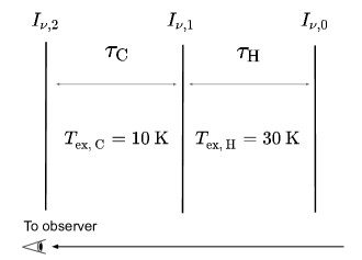
Figure 2: The toy model of molecular clouds with two $T_{\rm ex}$ layers. .

Such a model indicates that the column density ratio and the brightness temperature ratio estimated from optical depth would systematically deviate from the intrinsic ratios with a simplified one-layer assumption. This is because the measured excitation temperature of ¹²CN and ¹³CN $N=1\to 0$ will change with the optical depth with multiple $T_{\rm ex}$ layers. In our toy model, for $T_{\rm ex,H}=30$ K, $T_{\rm ex,C}=10$ K, $\tau_{\rm H}=\tau_{\rm C}=\tau$ and $R_{\rm{}^{12}C/^{13}C}$(intrinsic)=60, the intrinsic column density ratio and the intrinsic brightness temperature ratio will be $\sim$ 10% and $\sim$ 15% lower than the estimated ratios, respectively, when the optical depth of ¹²CN main component $\tau^{\rm main}_{\rm eff}\sim 1$ (i.e. $\sim$ 10% and $\sim$ 15% deviations from Eq. 4 and Eq. 5, respectively). When $\tau^{\rm main}_{\rm eff}\sim 1$, which is close to our measured $\tau$ of ¹²CN main components in our targets, such deviations will cause a $\sim$ 17% decrease of the derived $R_{\rm{}^{12}C/^{13}C}$ compared to the intrinsic ratio (red dashed line in Fig. 3 and details in Appendix B.4.1).

Multiple $T_{\rm ex}$ layers are significant when velocity spread is limited within linewidths of micro-turbulence and thermal motion, or when more than one fore/background cloud has identical $V_{\rm LSR}$. Observational evidence of self-absorption in $\rm{}^{12}CO$ (Enokiya et al., 2021), $\rm HCO^{+}$ (Richardson et al., 1986), and even $\rm{}^{13}CO$ (Sandell & Wright, 2010), which indicates multiple $T_{\rm ex}$ layers, are found in multiple sources of the CN sample (Wouterloot & Brand, 1989; Savage et al., 2002).

Other issues can also influence the derivation of $R_{\rm{}^{12}C/^{13}C}$. For example, the excitation temperature of ¹²CN may be higher than that of ¹³CN because of large optical depths and radiative trapping thermalizing the lines of the most abundant isotopologue at densities $\rm n=n_{crit,thin}(1-e^{-\tau})/\tau<n_{crit,thin}$. Non-LTE will also affect the derivation by changing the relative intensities between ¹²CN line components. These are beyond the scope of this work and wait for future investigation.

3.6 The method to derive $R_{\rm{}^{12}C/^{13}C}$ in extragalactic targets

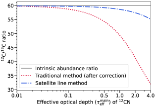
Figure 3: The theoretical values of derived $R_{\rm{}^{12}C/^{13}C}$ compared with the intrinsic values of $R_{\rm{}^{12}C/^{13}C}$ for the traditional HfS method and the satellite line method, varying with the optical depth of ¹²CN main component. We assume that $T_{\rm ex,H}=30$ K, $T_{\rm ex,C}=10$ K, $\tau_{\rm H}=\tau_{\rm C}=\tau$ and $R_{\rm{}^{12}C/^{13}C}$  (intrinsic) = 60.

The observations of CN isotopologues in the extragalactic star-burst galaxies provide $R_{\rm{}^{12}C/^{13}C}$ derived from the following equation (Henkel et al., 2014; Tang et al., 2019):

$$\frac{\rm{}^{12}C}{\rm{}^{13}C}=\frac{I_{\rm I,^{12}CN}\cdot\frac{\tau_{\rm I}}{1-e^{-\tau_{\rm I}}}+I_{\rm II,^{12}CN}\cdot\frac{\tau_{\rm II}}{1-e^{-\tau_{\rm II}}}}{1.082I_{\rm{}^{13}CN}}$$ (10)

Here, $I_{\rm I,^{12}CN}$ and $I_{\rm II,^{12}CN}$ are the total integrated intensities of ¹²CN $N=1\to 0$ $J=3/2\to 1/2$ and ¹²CN $N=1\to 0$ $J=1/2\to 1/2$, respectively. $\tau_{\rm I}$ and $\tau_{\rm II}$ are the total optical depth of the blended line components in $N=1\to 0$ $J=3/2\to 1/2$ and $J=1/2\to 1/2$, respectively.

This method will have the same deviation to $R_{\rm{}^{12}C/^{13}C}$ in Section 3.5 when the targets have complex excitation layers. Because of the large optical depth of ¹²CN and the small optical depth of ¹³CN, the effective $T_{\rm ex}$ of ¹²CN transitions will be smaller than that of ¹³CN in our toy model, which causes the underestimation of $R_{\rm{}^{12}C/^{13}C}$. In addition, the optical depth is derived from an equation similar to Eq. 5 (e.g., Eq. (1) in Tang et al., 2019). In our toy model, the $\tau_{\rm I}$ and $\tau_{\rm II}$ derived in this way may be overestimated. The $T_{\rm ex}$ layers will be more complex in reality than in our toy model, while differential excitation of the lines due to radiative trapping will only add to such complexity. Thus the $R_{\rm{}^{12}C/^{13}C}$ ratio estimated in this way still contains highly unclear uncertainties.

4 New method: deriving $\rm{}^{12}C/^{13}C$ and $\rm{}^{14}N/^{15}N$ with CN satellite lines and isotopologues

The satellite transitions of ¹²CN $N=1\to 0$, including $J=1/2\to 1/2,F=1/2\to 1/2$ (113.123 GHz) and $J=3/2\to 1/2,F=1/2\to 3/2$ (113.520 GHz) are expected to be optically-thin because the intrinsic relative line strengths of ¹²CN $N=1\to 0$ at these transitions are $\sim 3.6\%$ of that of the main component, which means an optical depth $\tau_{\rm s,^{12}CN}\sim 3.6\%$ of $\tau_{\rm main,^{12}CN}$.

Therefore, the effect of different $T_{\rm ex}$ layers on the derivation to $R_{\rm{}^{12}C/^{13}C}$ and $R_{\rm{}^{14}N/^{15}N}$ should be small based on our analysis. If the optical depth of the ¹²CN $N=1\to 0,J=3/2\to 1/2,F=1/2\to 3/2$ is less than 1, the theoretical deviation of the derived $R_{\rm{}^{12}C/^{13}C}$ will be $\lesssim$ 0.5%. This deviation is much smaller than the deviation in the traditional HfS method and can be ignored (see Fig 3).

The $R_{\rm{}^{12}C/^{13}C}$ can be derived from the following equation:

$$\frac{\rm{}^{12}C}{\rm{}^{13}C}=\frac{R^{\rm I/sum}_{13}}{R^{\rm I/sum}_{12}}\frac{I_{1}+I_{2}}{I_{\rm{}^{13}CN}}$$ (11)

Here, $R^{\rm I/sum}_{12}$ is the integrated intensity ratio between the sum of the two satellite lines and the sum of all the nine lines of ¹²CN $N=1\to 0$. $R^{\rm I/sum}_{13}$ is the ratio between the integrated intensities of the two strongest line components and that of all the components of ¹³CN $N=1\to 0$. $I_{1}$ and $I_{2}$ are the integrated intensities of ¹²CN $N=1\to 0$ $J=1/2\to 1/2,F=1/2\to 1/2$ and ¹²CN $N=1\to 0$ $J=3/2\to 1/2,F=1/2\to 3/2$, respectively. $I_{\rm{}^{13}CN}$ is the integrated intensity of the two strongest components of ¹³CN $N=1\to 0$. With the criteria in Section 2.3.2, if $I_{1}+I_{2}$ is larger than the 3-$\sigma$ value of the corresponding integrated intensity, we treat it as a detection.

This method still assumes a common $T_{\rm ex}$ among the energy levels involved in the lines used (i.e., the CTEX assumption, Mangum & Shirley, 2015, their Section 12). However, we sum up the integrated intensities of the two satellite lines to deduce the effect from hyperfine anomalies of ¹²CN, which has been observed in several studies (e.g., Bachiller et al., 1997; Hily-Blant et al., 2010).

Similarly, we can derive $R_{\rm{}^{14}N/^{15}N}$ with the same method by replacing the relative intensity ratio and the integrated line intensity of ¹³CN $N=1\to 0$ with those of C¹⁵N $N=1\to 0$.

5 Results

With the improved HfS method (the traditional method after corrections) listed in Section 3.3 and the new method (the satellite line method) in Section 4, we obtained the Galactic $R_{\rm{}^{12}C/^{13}C}$ and $R_{\rm{}^{14}N/^{15}N}$ gradients and add our new $R_{\rm{}^{12}C/^{13}C}$ and $R_{\rm{}^{14}N/^{15}N}$ results in the Galactic outer disk. We also discuss the differences between these gradients from different methods.

5.1 Line Detection and HfS fitting results

Among the total 15 sources, 11 targets have detections (S/N $>3$) of more than two $\rm{}^{12}CN$ $N=1\to 0$ satellite lines. One target, SUN15 18, has a detection of the main component of ¹²CN $N=1\to 0$. The other three targets only have non-detections of ¹²CN.

Two sources, G211.59 and WB89 380, show $\rm{}^{13}CN$ $N=1\to 0$ detections. G211.59 has a robust $\rm{}^{13}CN$ $N=1\to 0$ detection which has an S/N $\sim$ 8. The two blended main components of $\rm{}^{13}CN$ in WB89 380 are weakly detected with a total signal-to-noise ratio of $\sim$ 4.5. We did not detect ¹³CN  in WB89 391, at an $\sim 8\times$ better noise level than that of  Milam et al. (2005). Further comparison will be shown in Section 6.1.3. $\rm C^{15}N$ $N=1\to 0$ was only detected in G211.59.

We list the antenna temperatures of $\rm{}^{12}CN$, $\rm{}^{13}CN$ and $\rm C^{15}N$ $N=1\to 0$ in Table 4. The detected ¹²CN, ¹³CN and $\rm C^{15}N$ spectra are shown in Fig.  4. We show the spectra of ¹²CN and ¹³CN $N=1\to 0$ non-detected transitions in Appendix D.

For sources with more than two $\rm{}^{12}CN$ satellite line detections, our HfS fitting (Fig. 23 in Appendix  D) shows that $\tau_{\rm 12,main}<1$ in most of them (Table 4). Among them, three targets have large errors of $\tau_{\rm 12,main}$, so we do not include them in the following analysis.

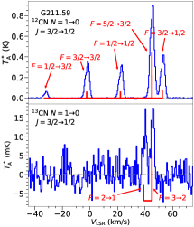
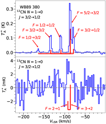
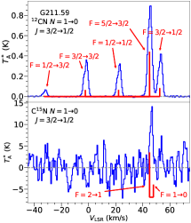
Figure 4: Spectra of $\rm{}^{12}CN$, $\rm{}^{13}CN$ and $\rm C^{15}N$ . The upper panels show spectra of $\rm{}^{12}CN$. The bottom panels are spectra of $\rm{}^{13}CN$ in the left panel, the middle panel, and $\rm C^{15}N$ in the right panel. Blue histograms show the spectra. Red solid lines show the relative location of hyperfine-structure transitions, labeled by red arrows. The gray dashed lines show the baseline of each spectrum. Left: The spectra of G211.59 with no smoothness, with the velocity resolution at $\sim$ 0.53 $\rm km\cdot s^{-1}$ Middle: The spectra of WB89 380 after smoothing four channels into one, with the velocity resolution at $\sim$ 2.15 $\rm km\cdot s^{-1}$ Right: The spectra of G211.59, showing the $\rm C^{15}N$ detection with the velocity resolution at $\sim$ 0.53 $\rm km\cdot s^{-1}$.

5.2 $\rm{}^{12}C/^{13}C$ gradient from the HfS method

With the antenna temperatures of $\rm{}^{12}CN$ and $\rm{}^{13}CN$ $N=1\to 0$, the $R_{\rm{}^{12}C/^{13}C}$ derived with Eq. 9 are listed in Table 4. We compare our newly measured $R_{\rm{}^{12}C/^{13}C}$ with those from CN observations reported in Savage et al. (2002); Milam et al. (2005). We update the Galactocentric distances of their targets and re-derive their $R_{\rm{}^{12}C/^{13}C}$ with Eq. 9. In Fig. 5 (a), we show the Galactic $R_{\rm{}^{12}C/^{13}C}$ gradients based on $\rm{}^{12}CN/^{13}CN$ derived from Eq. 9, which is systematically lower than the gradient reported by Milam et al. (2005).

Table 4: $\rm{{}^{12}C/^{13}C}$ and $\rm{}^{14}N/^{15}N$ ratios in our targets (The traditional HfS method).

Sources	$\tau_{\rm main}$	$T_{\rm A,^{12}CN}^{\star}$	$T_{\rm A,^{13}CN}^{\star}$	$\rm{{}^{12}C/^{13}C}$	$T_{\rm A,C^{15}N}^{\star}$	$\rm{}^{14}N/^{15}N$
		($10^{-1}\,$K)	($10^{-3}\,$K)		($\rm{10^{-3}}\>$K)
G211.59	0.86 $\pm$ 0.03	7.85 $\pm$ 0.03	13.1 $\pm$ 1.7	52.2 $\pm$ 6.7	8.7 $\pm$ 1.6	166 $\pm$ 32
G37.350	0.6 $\pm$ 1.1	1.28 $\pm$ 0.09	$\leq$ 16	$\geq$ 6.1	$\leq$ 16	$\geq$ 13
G44.8	0.71 $\pm$ 0.66	1.58 $\pm$ 0.09	$\leq$ 13	$\geq$ 9.4	$\leq$ 16	$\geq$ 17
IRAS0245	0.87 $\pm$ 0.23	3.29 $\pm$ 0.06	$\leq$ 9.6	$\geq$ 30	$\leq$ 13	$\geq$ 46
SUN15 14N	-	$\leq$ 0.6	$\leq$ 3.6	-	$\leq$ 43	-
SUN15 18a	-	0.7 $\pm$ 0.1	$\leq$ 3.1	-	$\leq$ 30	-
SUN15 21b	0.56 $\pm$ 11	1.15 $\pm$ 0.20	$\leq$ 28	$\geq$ 3.0	$\leq$ 22	$\geq$ 8.4
SUN15 34	-	$\leq$ 0.6	$\leq$ 4.2	-	$\leq$ 48	-
SUN15 56b	1.33 $\pm$ 10	1.02 $\pm$ 0.08	$\leq$ 17	$\geq$ 6.0	$\leq$ 21	$\geq$ 12
SUN15 57b	0.63 $\pm$ 11	1.04 $\pm$ 0.11	$\leq$ 16	$\geq$ 5.1	$\leq$ 24	$\geq$ 8.1
SUN15 7W	-	$\leq$ 0.6	$\leq$ 4.3	-	$\leq$ 43	-
WB89 380	0.58 $\pm$ 0.05	4.22 $\pm$ 0.03	5.7$\pm$1.7	57$\pm$17	$\leq$ 5.2	$\geq$ 134
WB89 391	0.98 $\pm$ 0.12	3.62 $\pm$ 0.05	$\leq$ 10	$\geq$ 32	$\leq$ 12	$\geq$ 59
WB89 437	0.26 $\pm$ 0.07	4.97 $\pm$ 0.04	$\leq$ 5.3	$\geq$ 62	$\leq$ 5.8	$\geq$ 122
WB89 501	0.50 $\pm$ 0.40	2.02 $\pm$ 0.07	$\leq$ 13	$\geq$ 12	$\leq$ 17	$\geq$ 19

• Failed to do HfS fitting for satellite lines of ¹²CN $N=1\to 0$.

• Huge error bars of $\tau$ in these targets.

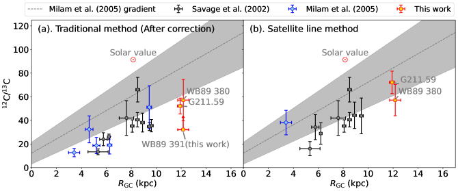
Figure 5: Ratio of $\rm{{}^{12}C/^{13}C}$ as a function of Galactocentric distance ($R_{\rm gc}$). (a): $R_{\rm{}^{12}C/^{13}C}$ derived from the corrected HfS method. (b). $R_{\rm{}^{12}C/^{13}C}$ derived from the optically-thin ¹²CN satellite line method. Black circles and blue diamonds are corrected values of results provided in Savage et al. (2002) and Milam et al. (2005), respectively. Red squares are our new $R_{\rm{}^{12}C/^{13}C}$ results of G211.59, WB89 380, and WB89 391. The grey dashed line with blocks shows the previous gradient provided in Milam et al. (2005) with 1-$\sigma$ error, which is $\rm{{}^{12}C/^{13}C=6.01(1.19)\it{D}_{\rm{GC}}\rm{+12.28(9.33)}}$. . The red circle with a central dot indicates the Solar value of $R_{\rm{}^{12}C/^{13}C}$ $=91.4\pm 1.3$ in this figure (Ayres et al., 2013), and in Figures  7 and 11.

5.3 $\rm{}^{14}N/^{15}N$ gradient from the HfS method

Fig. 6 (a) displays our Galactic $R_{\rm{}^{14}N/^{15}N}$ results from the HfS method. Besides $R_{\rm{}^{14}N/^{15}N}$ derived from the CN isotopologues with the HfS method (Adande & Ziurys, 2012), we show the $R_{\rm{}^{14}N/^{15}N}$ from other tracers together. We excluded targets for which $R_{\rm{}^{14}N/^{15}N}$ was calculated by multiplying a fitted gradient with $R_{\rm{}^{12}C/^{13}C}$ from the literature (e.g., Milam et al., 2005).

Our $R_{\rm{}^{14}N/^{15}N}$ gradient is also consistently lower than gradients reported in previous studies (e.g., Wilson & Rood, 1994; Adande & Ziurys, 2012; Colzi et al., 2018). We do revise $\rm{}^{12}CN/C^{15}N$ in Adande & Ziurys (2012) as what we do also for $\rm{}^{12}CN/^{13}CN$ in Savage et al. (2002) and Milam et al. (2005). In addition, Figure 6 shows the $R_{\rm{}^{14}N/^{15}N}$ derived from $\rm H^{13}CN/HC^{15}N$ multiplying $R_{\rm{}^{12}C/^{13}C}$ in two of our targets with both $R_{\rm{}^{12}C/^{13}C}$ and detected $\rm H^{13}CN$ and $\rm HC^{15}N$ $J=2\to 1$. More descriptions are in Appendix E.

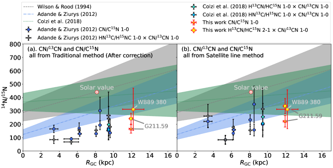
Figure 6: The Galactic $\rm{{}^{14}N/^{15}N}$ gradient. (a). The gradient with $R_{\rm{}^{14}N/^{15}N}$ derived from the CN HfS method and from $\rm H^{13}CN/HC^{15}N$ multiplying with $R_{\rm{}^{12}C/^{13}C}$ obtained by the HfS method. (b). The gradient with $R_{\rm{}^{14}N/^{15}N}$ from CN satellite line method and from $\rm H^{13}CN/HC^{15}N$ multiplying with $R_{\rm{}^{12}C/^{13}C}$ obtained by the satellite line method. The red star is $R_{\rm{}^{14}N/^{15}N}$ derived with CN $N=1\to 0$ of G211.59. The red squares are $R_{\rm{}^{14}N/^{15}N}$ from $\rm H^{13}CN/HC^{15}N$ multiplying $R_{\rm{}^{12}C/^{13}C}$ in G211.59 and WB89 380. For comparison, we show the $R_{\rm{}^{14}N/^{15}N}$ derived from $\rm CN/C^{15}N$ (Adande & Ziurys, 2012, royal blue circles); $\rm HN^{13}C/H^{15}NC\times^{12}C/^{13}C$ in  Adande & Ziurys (2012, grey crosses) and Colzi et al. (2018, deep sky blue hexagons); and $\rm H^{13}CN/HC^{15}N\times^{12}C/^{13}C$  (Colzi et al., 2018, turquoise hexagons). We also show the Galactic $R_{\rm{}^{14}N/^{15}N}$ gradients provided in  Wilson & Rood (1994, grey dashed line), Adande & Ziurys (2012, blue dashdot line) and Colzi et al. (2018, green dotted line). The corresponding color blocks show the 1-$\sigma$ ranges of these gradients. The red circle with a central dot shows the Solar value of $R_{\rm{}^{14}N/^{15}N}$$=440.5\pm 5.8$ from the protosolar nebula (Marty et al., 2011).

5.4 $\rm{}^{12}C/^{13}C$ and $\rm{}^{14}N/^{15}N$ gradients from CN $N=1\to 0$ satellite lines

Among eleven targets with the detection of ¹²CN $N=1\to 0$ main component, five of them have detected satellite lines. For targets in Savage et al. (2002) and Milam et al. (2005), we use the peak temperature of $J=3/2\to 1/2,F=1/2\to 3/2$ provided in Savage et al. (2002) and Adande & Ziurys (2012) to derive $R_{\rm{}^{12}C/^{13}C}$. In Table 5, we list the $R_{\rm{}^{12}C/^{13}C}$ of our targets derived in the optically-thin condition. Fig 5 (b) shows the Galactic $R_{\rm{}^{12}C/^{13}C}$ gradient from CN satellite lines. This gradient from optically thin satellite lines is systematically higher than the one derived from optical depth correction with HfS fitting.

In Table 5, we also show the $R_{\rm{}^{14}N/^{15}N}$ of our targets derived from optically-thin ¹²CN satellite lines and ¹³CN. Fig. 6 (b) shows the Galactic $R_{\rm{}^{14}N/^{15}N}$ gradient where all the ratios from CN isotopologues have been revised to the optically-thin results. The $R_{\rm{}^{14}N/^{15}N}$ derived from optically-thin CN satellite lines is higher than those from optical depth correction, which makes the Galactic $R_{\rm{}^{14}N/^{15}N}$ gradient higher than the one in Fig. 6 (a). In addition, we also show $R_{\rm{}^{14}N/^{15}N}$ derived from $\rm H^{13}CN/HC^{15}N$ multiplying $R_{\rm{}^{12}C/^{13}C}$, where $R_{\rm{}^{12}C/^{13}C}$ is obtained from ¹²CN optically-thin satellite lines, discussed in Section 6.2 and more details are in Appendix E.

Table 5: $\rm{{}^{12}C/^{13}C}$ and $\rm{}^{14}N/^{15}N$ ratios in our targets (The optically-thin $\rm{}^{12}CN$ satellite line method).

Sources	$I_{1}+I_{2}$	$I_{\rm{}^{13}CN}$	$\rm{{}^{12}C/^{13}C}$	$I_{\rm C^{15}N}$	$\rm{{}^{14}N/^{15}N}$
	($10^{-1}\,\rm K\cdot km\ s^{-1}$)	($\rm 10^{-3}\,K\cdot km\ s^{-1}$)		($\rm 10^{-3}\,K\cdot km\ s^{-1}$)
G211.59	5.90 $\pm$ 0.17	101 $\pm$ 13	72.2 $\pm$ 9.5	64 $\pm$ 12	222 $\pm$ 43
G37.350	$\leq$ 1.6	$\leq$ 87	-	$\leq$ 78	-
G44.8	$\leq$ 1.9	$\leq$ 79	-	$\leq$ 84	-
IRAS0245	0.76 $\pm$ 0.25	$\leq$ 35	$\geq$ 27	$\leq$ 44	$\geq$ 42
SUN15 21	$\leq$ 1.6	$\leq$ 91	-	$\leq$ 64	-
SUN15 56	$\leq$ 0.81	$\leq$ 49	-	$\leq$ 48	-
SUN15 57	$\leq$ 1.2	$\leq$ 49	-	$\leq$ 60	-
WB89 380	2.61 $\pm$ 0.20	56 $\pm$ 12	57 $\pm$ 13	$\leq$ 37	$\geq$ 174
WB89 391	1.06 $\pm$ 0.21	$\leq$ 36	$\geq$ 36	$\leq$ 38	$\geq$ 67
WB89 437	1.57 $\pm$ 0.22	$\leq$ 33	$\geq$ 59	$\leq$ 33	$\geq$ 116
WB89 501	$\leq$ 0.96	$\leq$ 51	-	$\leq$ 63	-

6 Discussion

6.1 The revision to the $\rm{}^{12}C/^{13}C$ gradient from the HfS method

In this section, we discuss the Galactic $R_{\rm{}^{12}C/^{13}C}$ and $R_{\rm{}^{14}N/^{15}N}$ gradients along the Galactic disc that are derived by applying the corrections mentioned above and our new method from CN isotopologues.

6.1.1 The updated Galactocentric distances

We employ the updated Galactic rotation curve from Reid et al. (2019). This choice leads to changes in the Galactocentric distances ($R_{\rm gc}$) of most sources in our sample compared to the values reported in Savage et al. (2002) and Milam et al. (2005). For most targets in the Galactic inner (outer) disk, $R_{\rm gc}$ increases (decreases) after applying the new rotation curve in Reid et al. (2019), with a typical difference of $\Delta R_{\rm gc}\sim 0-4$ kpc. One of our targets, WB89 437, has had its trigonometric parallax measured using VLBI in Reid et al. (2014), which indicated a Galactocentric distance of $R_{\rm gc}=13.10\pm 0.38$ kpc. This value is consistent with the value of $R_{\rm gc}=12.79\pm 0.38$ kpc derived from the Parallax-Based Distance Calculator.

Most of our targets are located in the anti-center direction, where the distance determination is not affected by confusion at the tangent point curve. However, most $R_{\rm gc}$ values in the literature (e.g., Brand & Wouterloot, 1995; Savage et al., 2002; Milam et al., 2005; Wouterloot et al., 2008; Giannetti et al., 2014) were derived from the Galactic rotation curve measured more than twenty years ago (e.g., Brand et al., 1986, 1988; Brand & Blitz, 1993; McNamara et al., 2000). This could introduce a strong bias in the derived abundance gradients.

In contrast, the distances derived from the updated rotation curve from Reid et al. (2019) not only benefit from more accurate measurements of the trigonometric parallax with VLBI, but also agree with the parallax-based distances of Galactic Hii regions that rely on Gaia EDR3 data (Méndez-Delgado et al., 2022) for nearby targets. The updated Galactocentric distance estimates lead to a systematic reduction in the number of targets with $R_{\rm gc}$>10 $\rm kpc$, yielding a steeper slope for the fitted gradient than the one in the literature where the previous, larger distances were used. For example, the Galactocentric distance of WB89 391 is now set to $\sim$12 kpc. This raises concerns about the previously reported high $R_{\rm{}^{12}C/^{13}C}$ value for this source (Milam, 2007) as this would seem reasonable for $R_{\rm gc}$ at $\sim$16 kpc, but not so for the updated distance of $\sim$12 kpc where a $\rm{}^{12}C/^{13}C$ $\sim$134 seems rather high. After the update, the Galactocentric distance of the sample is $R_{\rm gc}$<12 kpc. Fig. 11 in Appendix B.2 illustrates the changes in $R_{\rm{}^{12}C/^{13}C}$ before and after our revision.

6.1.2 Revised $R_{\rm{}^{12}C/^{13}C}$ after the Planck Equation and CMB contribution corrections

As expected, the $R_{\rm{}^{12}C/^{13}C}$ values (for the transitions of ¹²CN, and ¹³CN  $N$=1-0) derived using Equation 9 are systematically lower than those obtained using the R-J approximation and without considering the CMB temperature for targets in Savage et al. (2002); Milam et al. (2005), see Fig. 11. As we illustrated in Section 3.3.1 and Section 3.3.2, if the $T_{\rm ex}$ of ¹²CN is lower, the revision to $R_{\rm{}^{12}C/^{13}C}$ will be larger. The $T_{\rm ex}$ of ¹²CN $N=1\to 0$ of targets in Milam et al. (2005) is relatively lower ($T_{\rm ex}$$\sim 3-7$ K) than those ($T_{\rm ex}$$\sim 6-12$ K) from targets in Savage et al. (2002), so the revisions of targets in Milam et al. (2005) are larger than those in Savage et al. (2002). We note that this analysis assumes a common $T_{\rm ex}$ among the lines used. This CTEX assumption (see also Mangum & Shirley, 2015) is less constraining than LTE, and is likely to hold for the optically thin (or modestly optically thick) lines from rare CN isotopologues (unlike the more abundant isotopologues of CO where radiative trapping of more optically thick lines can yield different excitation temperatures among the isotopologues used).

6.1.3 Constraint on the outer Galactic disk – WB89 391

WB89 391 is located in the outer Galactic disc and was previously observed by Milam et al. (2005); Milam (2007). However, we did not detect the ¹³CN line for this target. As the original fluxes and their associated errors for the ¹²CN and ¹³CN lines were not reported in Milam et al. (2005); Milam (2007), we could only make a rough estimate of the noise level based on the $N=1\rightarrow 0$ spectra of ¹²CN and ¹³CN presented in Milam (2007).

At the rest frequency of $\rm{}^{13}CN$ $N=1\to 0$ main component (108.78 GHz), the beam sizes of IRAM 30-m and ARO 12-m are $\sim$ 22 ^′′ and $\sim$ 59 ^′′, respectively. Assuming a point source, the noise levels of $\rm{}^{13}CN$ (in flux density) are $\sim 0.02$ Jy and $\sim 0.16$ Jy for our measurement and the measurement in Milam et al. (2005), respectively. Therefore, our noise level is approximately eight times deeper than that reported in Milam et al. (2005).

The typical sizes of dense molecular cores have been shown to be about 0.1 pc (Wu et al., 2010), which is much smaller than our IRAM 30-m beamsize which corresponds to $\sim 1$ pc. Thus, we assume a point source distribution for $\rm{}^{12}CN$. In our study, we measured a $\rm{}^{12}CN$ flux density of about 2.4 Jy, while in Milam (2007), the flux density was about 2.3 Jy. The consistency between the two measurements suggests that this source is a compact target and the pointing directions of the observations were not severely offset from each other.

We also revisit the $\rm{}^{12}CN/^{13}CN$ ratio of WB89 391, using Equation 9 with the Planck expression and the CMB correction, based on the optical depth and the peak temperature reported in Milam et al. (2005) and Milam (2007). Our newly derived $R_{\rm{}^{12}C/^{13}C}$ for WB89 391 is $\sim$5.3 $\pm$ 1.7, which is about twenty-five times lower than the previously reported ratio of $\sim$134.

Our IRAM 30-m non-detection of WB89 391 sets a 3-$\sigma$ lower limit of $>$  36 for the $\rm{}^{12}CN/^{13}CN$ ratio, a result also supported by our recent NOEMA observation (Sun et al. in prep). Therefore, we recommend that the $\rm{}^{13}CN$ detection report in Milam et al. (2005) needs to be reconsidered for future analyses of the $R_{\rm{}^{12}C/^{13}C}$ gradient.

6.2 The impact of $\rm{}^{12}C/^{13}C$ gradient to the $\rm{}^{14}N/^{15}N$ one

The $R_{\rm{}^{12}C/^{13}C}$ gradient is commonly used to derive many other isotopic ratios. For example, by multiplying $R_{\rm{}^{12}C/^{13}C}$ (e.g., Wouterloot et al., 2008) with $\rm{}^{13}CO/C^{18}O$ and $\rm H^{13}CN/HC^{15}N$ (e.g., Colzi et al., 2018), or $\rm HN^{13}C/H^{15}NC$ (e.g., Adande & Ziurys, 2012; Colzi et al., 2018), it is possible to obtain $R_{\rm{}^{16}O/^{18}O}$ and $R_{\rm{}^{14}N/^{15}N}$, respectively.

The $\rm{}^{12}CN/^{13}CN$ ratios derived from optically thin satellite lines are systematically higher than those derived from optical depth correction. It will lead to systematically higher $R_{\rm{}^{14}N/^{15}N}$ when they are derived from multiplying $R_{\rm{}^{12}C/^{13}C}$ in optically-thin condition, compared with those multiplying the $R_{\rm{}^{12}C/^{13}C}$ from $\tau$-correction method.

In particular, we derive $R_{\rm{}^{14}N/^{15}N}$ of G211.59 from two methods: (a). Using $\rm H^{13}CN/HC^{15}N$ multiplying $R_{\rm{}^{12}C/^{13}C}$ (b). Directly using ¹²CN and C¹⁵N $N=1\to 0$. Using the $\rm H^{13}CN$ and $\rm HC^{15}N$ data from G211.59, we find that $\rm H^{13}C^{14}N/H^{12}C^{15}N=4.7\pm 2.5$. Using method (a), if we adopt that $R_{\rm{}^{12}C/^{13}C}$ $=52.2\pm 6.7$ derived from the HfS method, we will get $R_{\rm{}^{14}N/^{15}N}$ $\sim 242\pm 40$. Otherwise, if we adopt that $R_{\rm{}^{12}C/^{13}C}$ $=72.2\pm 9.5$ derived from the optically-thin satellite line method, we will have $R_{\rm{}^{14}N/^{15}N}$ $=336\pm 57$, which is much higher than the first value of $R_{\rm{}^{14}N/^{15}N}$. Using method (b), we get $R_{\rm{}^{14}N/^{15}N}$ $=166\pm 32$ from the HfS method and $R_{\rm{}^{14}N/^{15}N}$ $=222\pm 43$ from the satellite line method. The $R_{\rm{}^{14}N/^{15}N}$ from optical-thin satellite lines is also higher than the one from the HfS method. There is a discrepancy between the $R_{\rm{}^{14}N/^{15}N}$ values obtained using the method that directly uses CN isotopes and the method that relies on $R_{\rm{}^{12}C/^{13}C}$ as a conversion factor. This discrepancy persists regardless of whether we employ the HfS method or the optical-thin method, and it may be attributed to astrochemistry effects.

Recently, new $R_{\rm{}^{14}N/^{15}N}$ measurements on the Galactic outer disk were reported by Colzi et al. (2022). They obtained the $R_{\rm{}^{14}N/^{15}N}$ value by computing the abundance ratios of $\rm H^{13}CN/HC^{15}N$ and $\rm HN^{13}C/H^{15}NC$, which were then multiplied by the $R_{\rm{}^{12}C/^{13}C}$ gradient value provided in Milam et al. (2005). This work does not include corrections to astro-chemical effects on HCN isotopologues, and the $\rm{}^{14}N/^{15}N$ ratios derived from their analysis are systematically higher than ours. Particularly, the Galactic chemical evolution model in Colzi et al. (2022) shows lower $R_{\rm{}^{14}N/^{15}N}$ values in the Outer disk ($R_{\rm{}^{14}N/^{15}N}$ $\sim$250-400 at $R_{\rm gc}$ $\sim$ 12 kpc) than those derived from their observations, but model predictions remain consistent with $R_{\rm{}^{14}N/^{15}N}$ derived in this work.

However, WB89 391 induces a strong bias to the $R_{\rm{}^{12}C/^{13}C}$ gradient in Milam et al. (2005) which then propagates to the $R_{\rm{}^{14}N/^{15}N}$  gradient, making $R_{\rm{}^{14}N/^{15}N}$ ratios highly overestimated in the Galactic outer disk. If instead, the $\rm H^{13}CN/HC^{15}N$ and $\rm HN^{13}C/H^{15}NC$ ratios were multiplied by the $R_{\rm{}^{12}C/^{13}C}$ values obtained from optically-thin CN satellite lines in our work, the resulting $R_{\rm{}^{14}N/^{15}N}$ would be more consistent with our measurement of $R_{\rm{}^{14}N/^{15}N}$ derived from $\rm{}^{12}CN/C^{15}N$, with a small discrepancy possibly due to astrochemical effects.

6.3 Comparing CN with optically thin isotopic ratio tracers

Among the current tracers to derive $R_{\rm{}^{12}C/^{13}C}$, the abundance ratio of CO isotopologues (i.e., $\rm{}^{12}C^{18}O/^{13}C^{18}O$) have been adopted in plenty of Galactic targets, which gives a reliable sample size. In addition, $\rm C^{18}O$ and $\rm{}^{13}C^{18}O$ lines are expected to be optically thin, which will significantly reduce the effect of different excitation layers (similar to CN isotopologues, see Section 3.5).

We select $R_{\rm{}^{12}C/^{13}C}$ derived from $\rm{}^{12}C^{18}O/^{13}C^{18}O$ with enough signal-to-noise ratios provided in the literature (Langer & Penzias, 1990, 1993; Wouterloot & Brand, 1996; Giannetti et al., 2014) and combine them with our $R_{\rm{}^{12}C/^{13}C}$ derived from $\rm{}^{12}CN/^{13}CN$, shown in Fig.  7. The Galactocentric distances of all targets are derived with the same Galactic rotation curve model, following Reid et al. (2019).

Fig. 7 (a) overlays $R_{\rm{}^{12}C/^{13}C}$ of Galactic outer disk clouds derived with the traditional method (the CN $\tau$-correction method, $R_{\rm{}^{12}C/^{13}C}$ re-calculated with data from Savage et al. (2002) and Milam et al. (2005)), and $R_{\rm{}^{12}C/^{13}C}$ derived from $\rm{}^{12}C^{18}O/^{13}C^{18}O$ collected in the literature. The $R_{\rm{}^{12}C/^{13}C}$ ratios derived from $\rm{}^{12}CN/^{13}CN$ (the traditional method) appear systematically lower than that derived from the $\rm C^{18}O/^{13}C^{18}O$ method.

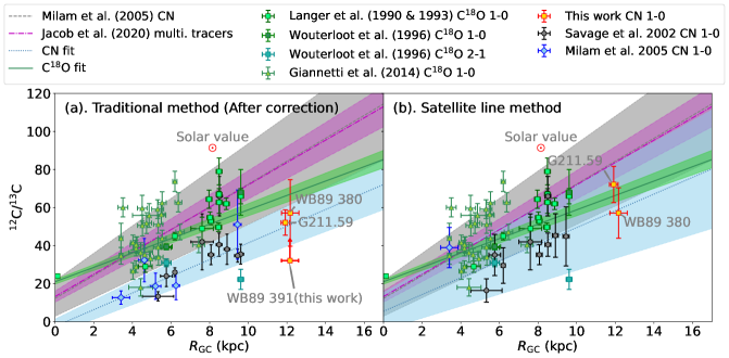
Figure 7: The $R_{\rm{}^{12}C/^{13}C}$  ratios obtained from different tracers. Left: The ratios derived from $\rm{}^{12}CN/^{13}CN$ with the traditional method. Right: The ratios derived from $\rm{}^{12}CN/^{13}CN$ with the optically-thin satellite line method. The grey dots, blue diamonds, and red squares are the $\rm{}^{12}CN/^{13}CN$ of targets in Savage et al. (2002), Milam et al. (2005), and in this work, respectively. The spring-green squares, sea-green squares, and yellow-green triangles are $\rm C^{18}O/^{13}C^{18}O$ at their $N=1\to 0$ transitions of targets in Langer & Penzias (1990, 1993), Wouterloot & Brand (1996) and Giannetti et al. (2014), respectively. The light-sea-green squares are $\rm C^{18}O/^{13}C^{18}O$ at their $N=2\to 1$ transitions in Wouterloot & Brand (1996). The grey dashed line shows the previous $\rm{}^{12}CN/^{13}CN$ gradient provided in Milam et al. (2005). The magenta dash-dotted line refers to the previous Galactic $\rm{}^{12}C/^{13}C$ gradient fitted with ratios derived from multiple tracers, provided in Jacob et al. (2020). The green solid line and the blue dotted line refer to the linear fitting curves of $R_{\rm{}^{12}C/^{13}C}$ from $\rm{}^{12}C^{18}O/^{13}C^{18}O$ and $\rm{}^{12}CN/^{13}CN$, respectively. The color blocks show the 1-$\sigma$ error range of corresponding linear-fitting curves.

Fig. 7 (b) shows the same comparison as Fig. 7 (a), but now $R_{\rm{}^{12}C/^{13}C}$ is derived with the Satellite-line method. The satellite line method seems to produce $R_{\rm{}^{12}C/^{13}C}$ better matching the $R_{\rm{}^{12}C/^{13}C}$ derived from $\rm C^{18}O/^{13}C^{18}O$, compared with those from the traditional method. Some $R_{\rm{}^{12}C/^{13}C}$ ratios have already been derived in the optically-thin condition in Savage et al. (2002), which do not change between Fig. 7 (a) and Fig. 7 (b). These $R_{\rm{}^{12}C/^{13}C}$ ratios are consistent with $R_{\rm{}^{12}C/^{13}C}$ from $\rm C^{18}O/^{13}C^{18}O$.

In Fig. 7, we also show two previous linear fitted gradients. The previous $\rm{}^{12}CN/^{13}CN$ gradient provided in Milam et al. (2005) is highly overestimated because of the R-J approximation and the neglect of the CMB temperature. The magenta one shows the fitted Galactic $\rm{}^{12}C/^{13}C$ gradient with previous data points from multiple tracers in the literature, concluded in Jacob et al. (2020). This gradient is also influenced by the previously overestimated $\rm{}^{12}CN/^{13}CN$ ratios. In the outer disk, both the $\rm{}^{12}C^{18}O/^{13}C^{18}O$ and $\rm{}^{12}CN/^{13}CN$ are expected to be lower than what the two previous gradients predict.

While there is significant scatter from each individual tracer, a general trend of increasing $R_{\rm{}^{12}C/^{13}C}$ from the Galactic center to the outer disk is apparent. The results based on the CO isotopologues also show a dependence on the chosen $J-$transition, i.e., $R_{\rm{}^{12}C/^{13}C}$ derived from the $J=1\to 0$ transition does not match with those obtained from the $J=2-\to 1$ lines (Wouterloot & Brand, 1996), likely due to differential excitation from clouds (Jacob et al., 2020). The two new data points from our survey, G211.59, and WB89 380, match both increasing gradients fitted from CN and CO isotopologues. Recently, Yan et al. (2023) provide $\rm{}^{12}C^{34}S/^{13}C^{34}S$ ratios also show an increasing $R_{\rm{}^{12}C/^{13}C}$ gradient with $R_{\rm{}^{12}C/^{13}C}$$\sim 75$ at $R_{\rm gc}$ $\sim$ 10 kpc. Therefore, we would expect that the even further outer disk region ($R_{\rm gc}$$>$ 15 kpc) may have even higher $R_{\rm{}^{12}C/^{13}C}$ ratios if the low-metallicity fast rotators are not dominated in the chemical evolution in this region. However, more observations are required to really constrain the chemical evolution in the further outer disk. In Appendix F, we show the linear fitted functions of the Galactic $R_{\rm{}^{12}C/^{13}C}$ and $R_{\rm{}^{14}N/^{15}N}$ gradients based on measurements from optically-thin conditions shown in Fig. 7 (b) and Fig. 6 (b), respectively. However, it is highly risky to use $R_{\rm{}^{12}C/^{13}C}$ or $R_{\rm{}^{14}N/^{15}N}$ from the linear fitting gradients instead of the direct measurement in individual targets (more details in Appendix F).

6.4 Astrochemical effects

Although the satellite method can reduce the deviation of abundance ratio measurements (Fig. 7 (b)), astrochemical effects may still bias the measured molecular abundances. This can introduce additional discrepancies between $R_{\rm{}^{12}C/^{13}C}$ of the same target derived from different tracers, and that between different targets (thus in different chemical environments) but derived from the same tracer.

$\bullet$ UV self-shielding: When exposed to UV radiation, more abundant $\rm{}^{12}C$-bearing molecules can self-shield themselves in the inner clouds, making them less vulnerable to destruction by UV photons. On the other hand, the less abundant $\rm{}^{13}C$-bearing isotopologues would be more easily destroyed even in the dense interior of clouds. This self-shielding effect can lead to an overestimation of $R_{\rm{}^{12}C/^{13}C}$  in emission line pairs such as $\rm C^{18}O$ and $\rm{}^{13}C^{18}O$, or $\rm CN$ and $\rm{}^{13}CN$ (van Dishoeck & Black, 1988; Röllig & Ossenkopf, 2013). Given the high localization of strong Photon-Dominated Regions (PDRs) around O stars in molecular clouds ($\rm L\leq$0.1 pc), such FUV-induced fractionization effects cannot affect globally-averaged isotopologue ratios over galaxy-sized molecular gas reservoirs, but they can affect local ISM regions like those observed in our study.

$\bullet$ Depletion: In dense and well-shielded regions, the temperature of dust can drop below the CO condensation temperature, typically around 17 K (e.g., Nakagawa, 1980). As a result, CO isotopologues freeze out onto the surface of dust grains (e.g., Willacy et al., 1998; Savva et al., 2003; Giannetti et al., 2014; Feng et al., 2020). Observations suggest that the depletion factors of $\rm{}^{12}C^{18}O$ and $\rm{}^{13}C^{18}O$ vary with density or temperature, but no systematic differences have been found (Savva et al., 2003; Giannetti et al., 2014).

$\bullet$ Chemical fractionation: In addition, the difference between the zero-point energy of $\rm{}^{12}CO$ and $\rm{}^{13}CO$ causes the carbon isotopic fractionation reactions (e.g.  Watson et al., 1976; Langer et al., 1984):

$${}^{13}{\rm C}^{+}+\hskip 2.84544pt^{12}{\rm CO}\leftrightarrow\hskip 2.84544pt^{13}{\rm CO}+\hskip 2.84544pt^{12}{\rm C}^{+}+35\hskip 2.84544pt{\rm K}$$ (12)

The CN isotopologues have a similar effect (Kaiser et al., 1991; Roueff et al., 2015):

$${}^{13}{\rm C}^{+}+\hskip 2.84544pt^{12}{\rm CN}\leftrightarrow\hskip 2.84544pt^{13}{\rm CN}+\hskip 2.84544pt^{12}{\rm C}^{+}+31.2\hskip 2.84544pt{\rm K}$$ (13)

Both gas-phase and grain-phase chemical networks have been adopted to model such fractionation effects on CO and CN molecules (e.g.  Smith & Adams, 1980; Roueff et al., 2015; Colzi et al., 2020; Loison et al., 2020). The experiments in Smith & Adams (1980) show $\rm{}^{13}C$ and $\rm{}^{18}O$ fractionation with a temperature $\lesssim$ 80 K. Ritchey et al. (2011) suggest that $\rm{}^{12}CO/^{13}CO$ and $\rm{}^{12}CN/^{13}CN$ evolution have inverse trends in the fractionation model in diffuse gas. Gas-phase models in Roueff et al. (2015) show that the diversion of $\rm{}^{12}CN/^{13}CN$ from original $\rm{}^{12}C/^{13}C$ is not significant with a temperature $\sim 10$ K. These models show stable $\rm C^{14}N/C^{15}N$ with an evolution time larger than $10^{6}$ years. This is consistent with the fractionation work containing gas and dust (Colzi et al., 2018), where the $\rm{}^{12}CN/^{13}CN$ becomes stable after an evolution time $\sim 10^{7}$ years. Recent results in Colzi et al. (2022) further find that nitrogen fractionation partly contributes to the scatter in the $R_{\rm{}^{14}N/^{15}N}$ measurements, while higher angular resolution observations are needed to disentangle local effects from nucleosynthesis contribution.

A detailed astrochemical study of the molecules used in such Galactic isotope ratio surveys, subjected to the varying far-UV radiation, cosmic ray, and pressure environments found in the sources used for such surveys will be particularly valuable. Should any $R_{\rm gc}$-systematic astrochemistry effects be found, such a study could yield valuable corrections to the (isotopologue)$\rightarrow$(isotope) abundance ratio conversion and reduce the scatter in Figure 7.

6.5 Comparing with abundance ratios from stars

The $R_{\rm{}^{12}C/^{13}C}$ ratio can also be measured from stars. Botelho et al. (2020) found local $R_{\rm{}^{12}C/^{13}C}$  values of $\sim 70-100$ in 63 Solar twins, higher than those derived from the interstellar medium ($R_{\rm{}^{12}C/^{13}C}$$\sim 40-60$ with $R_{\rm gc}$ $\sim$ 8 kpc). Recently, Zhang et al. (2021) found an $R_{\rm{}^{12}C/^{13}C}$ ratio of $97^{+25}_{-18}$ in an isolated brown dwarf with an age of $\sim 125$ Myr. This value is similar to the ratio found in the Sun (Ayres et al., 2013) and higher than the previously measured $R_{\rm{}^{12}C/^{13}C}$ ratio in the Solar neighborhood (Milam et al., 2005).

This is reasonable since abundance ratios measured from stars reflect the abundance of their parental ISM typically several billion years ago, which may be different from those in the local ISM because of stellar moving and the time evolution of $R_{\rm{}^{12}C/^{13}C}$. Recent studies based on Gaia and LAMOST data reveal that young ($<$100 Myr) stellar clusters in the Solar neighbourhood exhibit a variety of metallicity in their member stars, which indicates strong inhomogeneous mixing or fast star formation (Fu et al., 2022). These young clusters span a wide range of age and non-circular orbits, indicating multiple spatial origins (Fu et al., 2022).

6.6 Homogeneous mixing in the Solar neighbourhood

Optical spectroscopic observations of N and O towards Galactic Hii regions indicate well-mixed gas in the Galactic plane(e.g., Esteban et al., 2022), at least in the second and the third quadrants (Arellano-Córdova et al., 2020). Fig. 29 in Appendix G shows the location of those Hii regions and molecular clouds with $R_{\rm{}^{12}C/^{13}C}$ in this work. Most targets are located in the same quadrants as those Hii regions, indicating similar abundance ratios at the same Galactic radii.

However, these studies only consider the major isotopes of carbon and nitrogen, and the behavior of the rare isotopes $\rm{}^{13}C$ and $\rm{}^{15}N$ may not be the same as that of the major isotopes. In fact, the production and enrichment of these rare isotopes often involve different mechanisms from those of the major isotopes, such as novae (e.g., Romano & Matteucci, 2003; Cristallo et al., 2009; Romano, 2022). Furthermore, molecular tracers can be affected by additional chemical biases that may increase the scatter in measured abundances compared to those obtained from stellar tracers.

6.7 Future prospects

Our analysis of the different methods used to derive $R_{\rm{}^{12}C/^{13}C}$ and $R_{\rm{}^{14}N/^{15}N}$ indicates that the radiative transfer conditions may play an important role in affecting the basic assumptions of those methods. In particular, deriving isotopic ratios from lines of two molecular transitions with significantly different optical depth values (e.g., ¹²CN and ¹³CN $N=1\to 0$ main components, with $\tau$$\sim$1 and $\tau$$\sim$0.01, respectively) after performing optical depth corrections is highly non-trivial because of the expected non-uniform excitation conditions within the sources.

For the Galactic targets, parts of the $R_{\rm{}^{12}C/^{13}C}$ and $R_{\rm{}^{14}N/^{15}N}$ have been derived from $\rm{}^{12}CN/^{13}CN/C^{15}N$ (Savage et al., 2002; Milam et al., 2005; Adande & Ziurys, 2012) or $\rm{}^{14}NH_{3}/^{15}NH_{3}$ (Chen et al., 2021), with optical depth correction. After correcting the results using the full Planck function approximation and including the $T_{\rm CMB}$, the results are still subjected to the uncertainties of the underlying line excitation structure of the sources. It is always preferable to use the optically-thin line components, such as $\rm C^{18}O/^{13}C^{18}O$ or the optical-thin satellite lines of ¹²CN and $\rm{}^{14}NH_{3}$ with their isotopologues to derive $R_{\rm{}^{12}C/^{13}C}$ and $R_{\rm{}^{14}N/^{15}N}$ in Galactic targets.

For extragalactic sources the $R_{\rm{}^{12}C/^{13}C}$ can be derived from the $\rm{}^{12}CN/^{13}CN$ with optical depth correction (Henkel & Mauersberger, 1993; Henkel et al., 2014; Tang et al., 2019) but this method has the same issues as those used in the Milky Way, and it is hard to separate the optically-thin satellite line from the blended ¹²CN line components. It is better to use isotopologues with optically thin transitions (e.g., $\rm C^{18}O/^{13}C^{18}O$) for deriving isotopic ratios, but this requires longer integration time with high sensitivity instruments. According to our 2/15 detection rate of $\rm{}^{13}CN$ with an integration time $\sim 0.5-10$ hours of our targets (see in Table 1, 4 and 5), we suggest that an observing time of more than six hours may be required to detect $\rm{}^{13}C^{18}O$ in the targets of the outer disk with a sensitivity similar to that of IRAM 30-m.

On the other hand, all the current methods are based on LTE assumptions. Non-LTE will not only cause different excitation between isotopologues but also change the relative intensities of hyperfine structures (e.g., Henkel et al., 1998). These issues will be examined by the non-LTE models in the future.

7 Conclusions

We examine the assumptions and shortcomings of three different methods used to derive $R_{\rm{}^{12}C/^{13}C}$ from $\rm{}^{12}CN/^{13}CN$ namely: (a) the one using HfS fitting to do optical-depth correction of ¹²CN, adopted in the literature, (b) the improved $\tau$-correction method incorporating the Planck radiation temperature and the CMB contribution, (c) the method deriving $R_{\rm{}^{12}C/^{13}C}$ from the ratio of optically-thin ¹²CN satellite lines and ¹³CN lines. We also point out the similar issues of the methods of deriving $R_{\rm{}^{14}N/^{15}N}$ from ¹²CN and C¹⁵N. We observed $\rm{}^{12}CN$, $\rm{}^{13}CN$, and $\rm C^{15}N$ $N=1\to 0$ towards 15 molecular clouds on the outer Galactic disk ($R_{\rm gc}\sim\rm 12\ kpc-24\ kpc$). The Galactic $R_{\rm{}^{12}C/^{13}C}$ and $R_{\rm{}^{14}N/^{15}N}$ gradients obtained from different methods are shown by combining $R_{\rm{}^{12}C/^{13}C}$ and $R_{\rm{}^{14}N/^{15}N}$ derived from our new observations and those in the literature revised by our improved methods. Our results are as follows:

(i). The current method for deriving $\rm{}^{12}CN/^{13}CN$ in the literature adopts the Rayleigh-Jeans approximation and neglects the CMB, which then highly overestimates $R_{\rm{}^{12}C/^{13}C}$ when the excitation temperature of ¹²CN lines is $<$10 K. The improved $\tau$-correction method using the Planck equation and considering the CMB avoids these systematic overestimates, however, it still adopts the assumption of uniform excitation conditions. We show the latter still yields the under-estimate of $R_{\rm{}^{12}C/^{13}C}$ using a simple 2-phase excitation model. Scaling the intensity ratio of optically thin ¹²CN satellite lines and ¹³CN to the column density ratio of $\rm{}^{12}CN/^{13}CN$ avoids the shortcomings of the other two methods and is a better method for deriving reliable $R_{\rm{}^{12}C/^{13}C}$ from CN isotopologues.

(ii). Our method requires long integration time. For most targets, we can only set lower limits, but for the objects with the longer integration time (G211.59 and WB89 380), we measure $\rm{}^{12}C/^{13}C\sim$ 60. WB89 391, the target located at the outermost Galactic radius in the literature, shows no detection of $\rm{}^{13}CN$ from our IRAM 30-m data, which is inconsistent with the previous result reported in Milam et al. (2005). With $\sim$ 8$\times$ better sensitivity, our new data sets a lower limit of $R_{\rm{}^{12}C/^{13}C}$$\gtrsim 36$ in WB89 391 in the optically thin condition. We also give $R_{\rm{}^{14}N/^{15}N}$ $\sim$ 220 from $\rm{}^{12}CN/C^{15}N$ for one target and $R_{\rm{}^{14}N/^{15}N}$ $\sim$ 300 from $\rm H^{13}CN/HC^{15}N$ with $R_{\rm{}^{12}C/^{13}C}$ for two targets, at $R_{\rm gc}\sim 12$ kpc. These ratios are much lower than $R_{\rm{}^{14}N/^{15}N}$ derived from $\rm H^{13}CN/HC^{15}N$ or $\rm HN^{13}C/H^{15}NC$ multiplying $R_{\rm{}^{12}C/^{13}C}$ gradient in Milam et al. (2005), in better agreement with predictions of chemical evolution models.

(iii). The updated Galactic gradient of $R_{\rm{}^{12}C/^{13}C}$ (derived from $\rm{}^{12}CN/^{13}CN$ with $\tau$-correction) yields systematically lower values than previous results. The updated $R_{\rm{}^{12}C/^{13}C}$ gradient from CN optically-thin satellite lines is systematically steeper than the one from optical-depth correction. Such changes will regulate the Galactic $R_{\rm{}^{14}N/^{15}N}$ deriving from other ratios (e.g., $\rm H^{13}CN/HC^{15}N$) multiplying $R_{\rm{}^{12}C/^{13}C}$. In addition, the $R_{\rm{}^{12}C/^{13}C}$ obtained from $\rm{}^{12}CN/^{13}CN$ in the optically thin condition is more consistent with $R_{\rm{}^{12}C/^{13}C}$ from $\rm{}^{12}C^{18}O/^{13}C^{18}O$ than the one derived from the $\tau$-corrected method.

Data Availability

The $\rm{}^{12}C/^{13}C$ and $\rm{}^{14}N/^{15}N$ ratios from our new observations are listed in Table 4 and Table 5. The revised isotopic ratios from the targets in the literature can be derived with data provided in the corresponding works (Savage et al., 2002; Milam et al., 2005; Adande & Ziurys, 2012; Colzi et al., 2018; Langer & Penzias, 1990, 1993; Wouterloot & Brand, 1996; Giannetti et al., 2014), via Equations in this paper. The original IRAM 30-m data underlying this work will be shared on reasonable request to the corresponding author.

Appendix A The PDFs of estimated distances for our targets

We show the PDFs of the distances generated by the Parallax-Based Distance Calculator (Reid et al., 2016) for our targets in Fig. 8, and 9. Two of our targets, G211.59 and WB89 437, have direct parallax measurements of the water masers (Reid et al., 2019). So we use the parallax measurements to derive the Galactocentric distances for the two sources and do not show the PDFs of these two sources here.

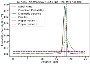
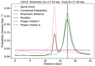
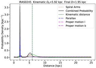
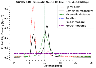
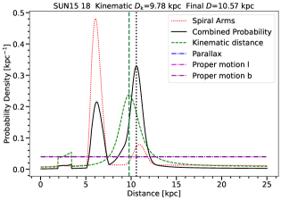
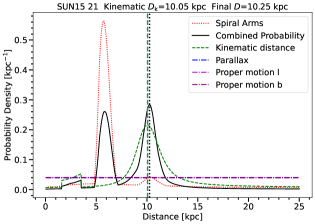
Figure 8: The probability distribution functions of the target distances. The red dotted curve, green dashed curve, blue dash-dot curve, magenta dash-dot curve, and purple dash-dot curve refer to the distance PDFs from Spiral arm distribution, kinematic methods, parallax, $l$ and $b$, respectively. The black solid curve is the combined PDF from all these PDFs. The green dashed vertical line shows the distance estimated only by kinematic PDF and the back dotted vertical line shows the final estimated distance.

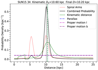
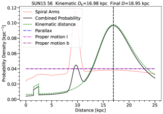
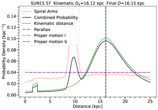
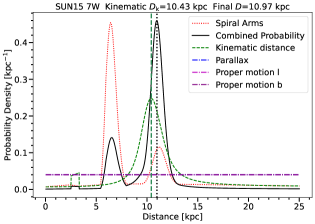
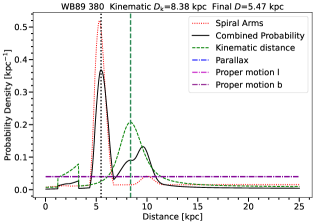
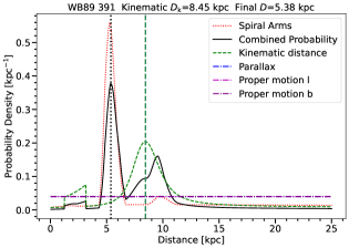
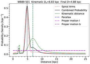
Figure 9: The probability distribution functions of the target distances (Continued).

Appendix B The derivation of a more complete the $R_{\rm{}^{12}C/^{13}C}$ formula

B.1 The derivation of $R_{\rm{}^{12}C/^{13}C}$ formula in the literature

In this section, we illustrate our derivation of $R_{\rm{}^{12}C/^{13}C}$. We assume that the element abundance ratio $R_{\rm{}^{12}C/^{13}C}$ equals the column density ratio between $\rm{}^{12}CN$ and $\rm{}^{13}CN$ (i.e. ignore the astrochemistry effects). The column density can be described as (Mangum & Shirley, 2015):

$$N_{\rm tot}=\frac{3h}{8\pi^{3}|\mu_{\rm lu}|^{2}}\frac{Q_{\rm tot}}{g_{\rm u}}\frac{{\rm exp}(\frac{E_{\rm u}}{kT_{\rm ex}})}{{\rm exp}(\frac{h\nu}{kT_{\rm ex}})-1}\int\tau_{\nu}dv$$ (14)

Here, $N_{\rm tot}$ means the total molecular column density of all energy levels. $h$ is the Planck constant and $\mu_{\rm lu}$ represents the dipole moment matrix element. $Q_{\rm tot}$ represents the rotational partition function. $E_{\rm u}$ and $g_{\rm u}$ represent the energy level and the degeneracy of the upper-level u, respectively. In this work, we assume the molecular structures of $\rm{}^{12}CN$ and $\rm{}^{13}CN$ are similar so the difference between $\mu_{\rm lu}$, $Q_{\rm tot}$, $E_{\rm u}$ and $g_{\rm u}$ can be ignored. We also assume a common excitation temperature $T_{\rm ex}$. Then the column density ratio of ¹²CN and ¹³CN $N=1\to 0$ can be described as:

$$\frac{N_{\rm tot,^{12}CN}}{N_{\rm tot,^{13}CN}}=\frac{\int\tau_{\nu,\rm^{12}CN}dv}{\int\tau_{\nu,\rm^{13}CN}dv}=\frac{\tau_{12}}{\tau_{13}}$$ (15)

Here $\tau_{12}$ and $\tau_{13}$ represent the optical depth of $\rm{}^{12}CN$ and $\rm{}^{13}CN$ $N=1\to 0$, respectively. We can derive the column density ratio of the main components of $\rm{}^{12}CN$ and $\rm{}^{13}CN$ $N=1\to 0$ and then convert this ratio to the column density ratio of all the energy levels. We can set $R_{12}$ and $R_{13}$ as conversion factors from the main component to all states of $\rm{}^{12}CN$ and $\rm{}^{13}CN$, respectively. That means:

$$\frac{N_{\rm main,^{12}CN}}{N_{\rm tot,^{12}CN}}=R_{12},\quad\frac{N_{\rm main,^{13}CN}}{N_{\rm tot,^{13}CN}}=R_{13}$$ (16)

We will also have:

$$\frac{N_{\rm main,^{12}CN}}{N_{\rm main,^{13}CN}}=\frac{R_{12}\tau_{12}}{R_{13}\tau_{13}}=\frac{\tau_{\rm m,12}}{\tau_{\rm m,13}}$$ (17)

The $\tau_{\rm m,12}$ and $\tau_{\rm m,13}$ are the optical depth of the main component of $\rm{}^{12}CN$ and $\rm{}^{13}CN$, respectively.

On the other hand, the equation of radiative transfer for a uniform-excitation source is (e.g., Mangum & Shirley, 2015):

$$T_{\rm R}=f[J_{\nu}(T_{\rm ex})-J_{\nu}(T_{\rm bg})][1-e^{-\tau_{\nu}}]$$ (18)

Here $T_{\rm R}$ is the beam-averaged source radiation temperature with $f$ the source beam-filling factor and $T_{\rm bg}$ the background temperature here assumed to be the CMB at 2.73 K. The beam filling factor: f=$\Omega_{\rm s}/\Omega_{\rm mb}$, with $\rm\Omega_{\rm s}$=$\int_{\omega_{\rm s}}P_{\rm n}(\omega)\Psi_{\rm s}(\omega)d\omega_{s}$, where $P_{\rm n}$ is the beam pattern function, $\Psi_{\rm s}$ the normalised source brightness distribution function (see Kutner & Ulich, 1981, Equation 3) and $\omega_{\rm s}$ the solid angle range subtended by the source, while $\Omega_{\rm mb}$=$\int_{\omega_{\rm d}}P_{\rm n}d\omega$, with $\omega_{\rm d}$ the beam forward-pattern (typically Gaussian for the IRAM 30-m telescope at its operating frequencies, but not necessarily so for high-frequency sub-mm telescopes).

The $J_{\nu}(T)$ expression gives the Rayleigh-Jeans equivalent temperature, but after using the Planck function for the black body radiation:

$$T_{\rm b}=\frac{c^{2}}{2k_{\rm B}\nu^{2}}B_{\rm\nu}(T)=J_{\rm\nu}(T)\equiv\frac{\frac{h\nu}{k}}{e^{\frac{h\nu}{kT}}-1}$$ (19)

If the line is optically thin, Equation 18 becomes

$$T_{\rm R}=f[J_{\nu}(T_{\rm ex})-J_{\nu}(T_{\rm bg})]\tau_{\nu}$$ (20)

Insert Equation 20 into 14 and simplify the 14 as:

$$N_{\rm tot}={\rm A}({\rm mol},T_{\rm ex})\int\tau_{\nu}dv$$ (21)

Here the ${A}({\rm mol},T_{\rm ex})$ refers to all the parameters in Equation 14 to the left of the integral sign. Then we get:

$$N_{\rm tot}={\rm A}({\rm mol},T_{\rm ex})\int\frac{T_{\rm R}}{f[J_{\nu}(T_{\rm ex})-J_{\nu}(T_{\rm bg})]}dv$$ (22)

as the source-averaged column density, with $\langle N_{\rm tot}\rangle_{\rm beam}$=$fN_{\rm tot}$ being the beam-averaged column density. Here it is important to note that while line ratio excitation analysis can constrain the $T_{\rm ex}$ values, this cannot be done for the source beam filling factor unless independent source size estimates can be had (e.g. via past interferometric observations of the same molecules or concomitant line and/or continuum emitters (e.g. dust emission). Thus typically in the literature $\langle N_{\rm tot}\rangle_{\rm beam}$ is typically reported.

If the line has some modest optical depths, $N_{\rm tot}$ can still be derived after multiplying a $\tau$-correcting factor $\frac{\tau}{1-e^{-\tau}}$ (Goldsmith & Langer, 1999; Mangum & Shirley, 2015), yielding:

$$N_{\rm tot}=\frac{\tau}{1-e^{-\tau}}{\rm A}({\rm mol},T_{\rm ex})\int\frac{T_{\rm R}}{f[J_{\nu}(T_{\rm ex})-J_{\nu}(T_{\rm bg})]}dv$$ (23)

, but such corrections become unreliable for large line optical depths ($\tau$$\geq$2-3). For the small velocity range of the lines in this work ($\rm FWHM$$\sim$ $1.5-4$ $\rm km\,s^{-1}$), the optical depth correction factor, $A({\rm mol},T_{\rm ex})$, and $J(\nu,T_{\rm ex})$ factors can all be considered constant across the line width. Thus we can compute the velocity-averaged column density across the entire line profile (which yields the highest possible S/N ratio for spectral line observations) from Equation 23 as:

$$N_{\rm tot,V}=\frac{\tau}{1-e^{-\tau}}\frac{{\rm A}({\rm mol},T_{\rm ex})}{f[J_{\nu}(T_{\rm ex})-J_{\nu}(T_{\rm bg})]}\left[\frac{1}{\Delta V}\int T_{\rm R}dv\right]$$ (24)

For the $R_{\rm{}^{12}C/^{13}C}$ derivation, with $\rm{}^{12}CN$ $N=1\to 0$ optically thick and the $\rm{}^{13}CN$ $N=1\to 0$ optically thin (thus a $\tau$-correction factor only applies to ¹²CN), and$A({\rm mol},T_{\rm ex})$ and the source beam-filling factors $f$ identical between the two lines, we can write:

$$\frac{N_{\rm main,^{12}CN}}{N_{\rm main,^{13}CN}}=\frac{\tau}{1-e^{-\tau}}\frac{\int T_{\rm R,^{12}CN}dv}{\int T_{\rm R,^{13}CN}dv}$$ (25)

Now we consider the formula to calculate $R_{\rm{}^{12}C/^{13}C}$ used by Savage et al. (2002) and  Milam et al. (2005). The formula they used is:

$$\frac{\rm{}^{12}C}{\rm{}^{13}C}=\frac{(3/5)\tau_{\rm main}T_{\rm ex,^{12}CN}}{T^{\star}_{\rm R,^{13}CN}/\eta_{\rm c,^{13}CN}}$$ (26)

Here they erroneously set $\eta_{\rm c}$ as the beam efficiency, despite the $T^{\star}_{\rm R}$ temperature scale of the 12-m telescope being already corrected for all telescope efficiency factors (and of course atmospheric absorption). Here, $\tau_{\rm main}$ is the optical depth of the main component of $\rm{}^{12}CN$ and $T^{\star}_{\rm R,^{13}CN}$ is the measured radiation temperature of the $\rm{}^{13}CN$ main component and 3/5 is the conversion factor from the ratio of main components to the ratio of all levels.

To deduce Equation 26, we need to obtain a formula with $T_{\rm ex,^{12}CN}$, $\tau_{\rm main}$ and $T^{\star}_{\rm R,^{13}CN}$. We replace $T^{\star}_{\rm R,^{12}CN}$ by inserting Equation 20 into Equation 25:

$$\frac{N_{\rm main,^{12}CN}}{N_{\rm main,^{13}CN}}=\frac{\tau}{1-e^{-\tau}}\frac{\int f[J_{\nu}(T_{\rm ex})-J_{\nu}(T_{\rm bg})][1-e^{-\tau_{\nu}}]dv}{\int T_{\rm R,^{13}CN}dv}$$ (27)

Assuming the optical depth is nearly constant across the narrow line profile, we can further write:

$$\frac{N_{\rm main,^{12}CN}}{N_{\rm main,^{13}CN}} =\frac{\tau}{1-e^{-\tau}}\frac{f[J(T_{\rm ex})-J(T_{\rm bg})](1-e^{-\tau})}{T_{\rm R,^{13}CN}}$$ (28)

$$=\frac{\tau f[J(T_{\rm ex})-J(T_{\rm bg})]}{T_{\rm R,^{13}CN}}$$

If we regard $T^{\star}_{\rm R,^{13}CN}$ as the observed corrected source antenna temperature of the ¹³CN main component as reported by the (former) NRAO 12m-telescope we will have:

$$\frac{N_{\rm main,^{12}CN}}{N_{\rm main,^{13}CN}}=\frac{\tau[J(T_{\rm ex})-J(T_{\rm bg})]}{T^{\star}_{\rm R,^{13}CN}/f_{\rm{}^{13}CN}}$$ (29)

Assuming the ¹³CN beam filling factor $f=1$, and converting the column density at one transition to the total molecular gas column density, we obtain:

$$\frac{N_{\rm tot,^{12}CN}}{N_{\rm tot,^{13}CN}} =\frac{R_{13}\tau[J(T_{\rm ex})-J(T_{\rm bg})]}{R_{12}T^{\star}_{\rm R,^{13}CN}/(\eta_{\rm c,^{13}CN})}$$ (30)

$$\approx\frac{(3/5)\tau[J(T_{\rm ex})-J(T_{\rm bg})]}{T^{\star}_{\rm R,^{13}CN}}$$

Using the Rayleigh-Jeans approximation ($J(T)$$\approx T$) and ignoring CMB temperature $T_{\rm bg}$, yields the same equation as Equation 26, but without the erroneous $\eta_{\rm c}$ factor.

B.2 The effects of the R-J approximation and the $T_{\rm CMB}$ emission

In order to quantify the effect of the R-J approximation we derive the excitation temperature $T_{\rm ex}$ of $\rm{}^{12}CN$ $N=1\to 0$ for our targets, according to the following equation:

$$T^{\star}_{\rm A}=\eta_{\rm mb}f[J_{\nu}(T_{\rm ex})-J_{\nu}(T_{\rm bg})][1-e^{-\tau_{\nu}}]=\eta_{\rm mb}T_{\rm mb}$$ (31)

We assume that $T_{\rm bg}$=$T_{\rm CMB}$=2.73 K, with $T^{\star}_{\rm A}$ and $\tau_{\nu}$ of ¹²CN $N=1\to 0$ obtained from HfS fitting. The $T_{\rm ex}$ of ¹²CN is then derived from Eq. 31. The results are listed in Table 6. The mapping data of $\rm{}^{13}CO$ is used to estimate the filling factor $f$, with the assumption that the shape of targets is round with an area including all pixels having $T_{\rm mb,^{13}CO}>0.5\ T_{\rm mb,^{13}CO}^{\rm peak}$.

Table 6: $T_{\rm ex}$ of $\rm{}^{12}CN$ $N=1\to 0$ in our targets.

Sources	$T_{\rm ex,^{12}CN}$
	(K)
G211.59	4.61 $\pm$ 0.08a
G37.350	3.5 $\pm$ 1.5
G44.8	3.7 $\pm$ 1.0
IRAS0245	3.6 $\pm$ 0.3
SUN15 14N	-
SUN15 18	-
SUN15 21b	3 $\pm$ 10
SUN15 34	-
SUN15 56b	2.9 $\pm$ 1.4
SUN15 57b	3.1 $\pm$ 7.7
SUN15 7W	-
WB89 380	4.34 $\pm$ 0.18
WB89 391	4.16 $\pm$ 0.20
WB89 437	6.7 $\pm$ 1.1
WB89 501	4.0 $\pm$ 1.0

• A filling factor f=1 (and $\eta_{c}$=1) is assumed due to the unresolved mapping data, thus yielding a minimum $T_{\rm ex}$ value.

• Huge errors are shown for SUN15 21, SUN15 56, and SUN15 57, which means that the ratio limit results for these three sources are not credible.

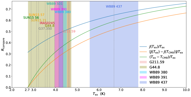
Figure 10: The effects of Rayleigh-Jeans approximation and background temperature. The solid lines show the change of $R_{\rm compare}$ with the excitation temperature $T_{\rm ex}$, in the condition a (blue), condition b (green), and condition c (orange). The dashed lines show the $T_{\rm ex}$of $\rm{}^{12}CN$ $N=1\to 0$ in our sources and colorful blocks show the error range of $T_{\rm ex}$.

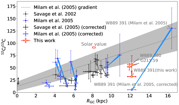
Figure 11: Galactic $R_{\rm{}^{12}C/^{13}C}$ gradients derived from CN, before and after our corrections. The grey dots, blue diamonds, and red squares refer to results from Savage et al. (2002), Milam et al. (2005), and this work, respectively. The symbols filled with darker colors refer to previous values in the literature and those filled with lighter colors are the corrected values. The arrows show the change.

We define the ratios between the revised $R_{\rm{}^{12}C/^{13}C}$ and the previous $R_{\rm{}^{12}C/^{13}C}$, labeled as $R_{\rm compare}$. Then we consider three conditions:

(a) Using the Planck equation and without $T_{\rm CMB}$:

$$R_{\rm compare,a}=\frac{R_{\rm 12C13C,Planck\ eq,no\ CMB}}{R_{\rm 12C13C,R-J\ approx,no\ CMB}}=\frac{J(T_{\rm ex})}{T_{\rm ex}}$$ (32)

(b) With R-J approximation and with $T_{\rm CMB}$:

$$R_{\rm compare,b}=\frac{R_{\rm 12C13C,R-J\ approx,CMB}}{R_{\rm 12C13C,R-J\ approx,no\ CMB}}=\frac{T_{\rm ex}-T_{\rm CMB}}{T_{\rm ex}}$$ (33)

(c) Using the Planck equation and with $T_{\rm CMB}$:

$$R_{\rm compare,c}=\frac{R_{\rm 12C13C,Planck\ eq,CMB}}{R_{\rm 12C13C,R-J\ approx,no\ CMB}}$$ (34)

$$=\frac{J(T_{\rm ex})-J(T_{\rm CMB})}{T_{\rm ex}}$$

Fig.  10 shows the change of $R_{\rm compare}$ with $T_{\rm ex}$. For all the conditions $R_{\rm compare}$ will decrease when $T_{\rm ex}$decreases. In condition (a), $R_{\rm compare}$ > 0.95, which means the decrease of $R_{\rm{}^{12}C/^{13}C}$ after revision is $\leq 5$ %, for $T_{\rm ex}\gtrsim 53$ K. $R_{\rm compare}$ becomes $\sim 0.5$ for $T_{\rm ex}\sim 4.3$ K. In condition (b), $R_{\rm compare}$ > 0.95 and $\sim 0.5$ for $T_{\rm ex}\gtrsim 54$ K and $\sim 6.3$ K, and $\sim$ 3.1 K, respectively. For case (c), used in this work, it is $R_{\rm compare}$>0.95, $\sim 0.5$, and $\sim$0.1, for $T_{\rm ex}$$\gtrsim$70 K, $\sim$6.3 K, and $\sim$ 3.1 K, respectively. We conclude that if $T_{\rm ex}$$\leq$10 K, the Planck equation and the CMB must be considered to derive $R_{\rm{}^{12}C/^{13}C}$ from $\rm{}^{12}CN/^{13}CN$.

In Fig. 11, we show how the effects of the R-J approximation and the CMB temperature will revise the previous Galactic $\rm{}^{12}CN/^{13}CN$ gradient derived from the HfS method. After the Galactocentric distance revision, the targets have a change of $R_{\rm gc}$ at $\sim 0-4$ kpc, and the $R_{\rm gc}$ are limited to $\lesssim$ 12 kpc. The values of $R_{\rm{}^{12}C/^{13}C}$ systematically decrease after the revision. Especially, the previous out-most constraint, $R_{\rm{}^{12}C/^{13}C}$ in WB89 391, has been in an unphysical region after the revision, which means the previous measurement of this target is highly doubtful.

B.3 The derivation of a $\tau$-corrected $R_{\rm{}^{12}C/^{13}C}$ formula

Table 7: $T_{\rm ex}$ of $\rm{}^{12}CN$ $N=1\to 0$ in targets of Savage et al. (2002) and Milam et al. (2005).

Sources	$T_{\rm ex,^{12}CN,pre.}$	$T_{\rm ex,^{12}CN,revis.}$
	(K)	(K)
W3(OH)	6.00 $\pm$ 0.50	5.41 $\pm$ 0.41
G34.3	6.00 $\pm$ 0.20	5.41 $\pm$ 0.16
W51M	12.4 $\pm$ 2.0	10.7 $\pm$ 1.6
NGC 7538	8.10 $\pm$ 0.50	7.13 $\pm$ 0.41
NGC 2024	7.30 $\pm$ 0.10	6.48 $\pm$ 0.08
W33	8.90 $\pm$ 0.40	7.79 $\pm$ 0.33
G29.9	5.10 $\pm$ 0.72	4.67 $\pm$ 0.59
G19.6	3.39 $\pm$ 0.08	3.27 $\pm$ 0.07
W31	6.95 $\pm$ 0.85	6.19 $\pm$ 0.70
G35.2	4.49 $\pm$ 0.40	4.17 $\pm$ 0.33
S156	6.6 $\pm$ 1.6	5.9 $\pm$ 1.3
WB89 391	2.90 $\pm$ 0.03	2.87 $\pm$ 0.02

Equation 30 contains the assumption that the filling factor $f=1$. However, in this work, we take a more simple consideration, namely we assume $T_{\rm ex}$ is the same for both $\rm{}^{12}CN$ and $\rm{}^{13}CN$ $N=1\to 0$ main components. Because the corresponding frequencies are so similar for these two components the now frequency-dependant expressions $J(T_{\rm ex})-J(T_{\rm bg})$ will also be very similar for the two lines (and of course the main beam efficiency factors $\eta_{\rm mb}$ as well). We assume the spatial distributions of these isotopologues are similar so that $f$ (or $\eta_{\rm c}$ for resolved-source observations) is the same. According to Eq. 31, we then have:

$$R_{\rm b}=\frac{T_{\rm b,^{12}CN}}{T_{\rm b,^{13}CN}}=\frac{f_{\rm{}^{12}CN}(1-e^{-\tau_{\rm m,12}})}{f_{\rm{}^{13}CN}(1-e^{-\tau_{\rm m,13}})}=\frac{1-e^{-\tau_{\rm m,12}}}{1-e^{-\tau_{\rm m,13}}}=\frac{T_{\rm mb,^{12}CN}}{T_{\rm mb,^{13}CN}}$$ (35)

Here $T_{\rm b,^{12}CN}$ and $T_{\rm b,^{13}CN}$ are the peaks of the brightness temperature of the main components of $\rm{}^{12}CN$ and $\rm{}^{13}CN$. We set $R_{\rm b}$=$T_{\rm b,^{12}CN}/T_{\rm b,^{13}CN}$, which is the brightness temperature ratio of the main components of $\rm{}^{12}CN$ and $\rm{}^{13}CN$. With the assumption that the filling factor of ¹²CN ($f_{\rm{}^{12}CN}$) equals the filling factor of ¹³CN ($f_{\rm{}^{12}CN}$), we have $R_{\rm b}$=$T_{\rm mb,^{12}CN}/T_{\rm mb,^{13}CN}$. $\tau_{\rm m,12}$ and $\tau_{\rm m,13}$ are the optical depths of the ¹²CN and ¹³CN main components, respectively. We also set:

$$R_{\rm 1213}=\frac{N_{\rm main,^{12}CN}}{N_{\rm main,^{13}CN}}=\frac{\tau_{\rm m,12}}{\tau_{\rm m,13}}$$ (36)

with $R_{\rm 1213}$=$N_{\rm main,^{12}CN}/N_{\rm main,^{13}CN}$ being the column density ratio between the main components of ¹²CN and ¹³CN $N=1\to 0$. Then we have $\tau_{\rm m,13}=\tau_{\rm m,12}/R_{\rm 1213}$. Inserting this into 35 yields:

$$R_{\rm b}=\frac{1-e^{-\tau_{\rm m,12}}}{1-e^{-\tau_{\rm m,12}/R_{\rm 1213}}},$$ (37)

which, solving for $R_{\rm 1213}$, it simply yields:

$$R_{\rm 1213}=-\frac{\tau_{\rm m,12}}{{\rm ln}[1-(1-e^{-{\tau_{\rm m,12}}})/R_{\rm b}]}$$ (38)

That is:

$$\frac{N_{\rm main,^{12}CN}}{N_{\rm main,^{13}CN}}=-\frac{\tau_{\rm m,12}}{{\rm ln}[1-\frac{T_{\rm mb,^{13}CN}}{T_{\rm mb,^{12}CN}}(1-e^{-{\tau_{\rm m,12}}})]}$$ (39)

We then convert the column density ratio of the main components to that of all levels of $\rm{}^{12}CN$ and $\rm{}^{13}CN$ $N=1\to 0$. That is:

$$\frac{\rm{}^{12}C}{\rm{}^{13}C} =\frac{N_{\rm tot,^{12}CN}}{N_{\rm tot,^{13}CN}}$$ (40)

$$=-\frac{R_{13}}{R_{12}}\cdot\frac{\tau_{\rm m,12}}{{\rm ln}[1-\frac{T_{\rm mb,^{13}CN}}{T_{\rm mb,^{12}CN}}(1-e^{-{\tau_{\rm m,12}}})]}$$

$$=-\frac{R_{13}}{R_{12}}\cdot\frac{\tau_{\rm m,12}}{{\rm ln}[1-\frac{T^{\star}_{\rm A,^{13}CN}/\eta_{\rm mb,^{13}CN}}{T^{\star}_{\rm A,^{12}CN}/\eta_{\rm mb,^{12}CN}}(1-e^{-{\tau_{\rm m,12}}})]}$$

Equation 40 is the one used in this work to derive $R_{\rm{}^{12}C/^{13}C}$ with optical-depth correction. There is no need to consider particular $T_{\rm ex}$ and filling factor $f$ (as long as they are common for the lines/species used) once we convert the measured antenna temperature $T^{\star}_{\rm A}$ to the main beam temperature $T_{\rm mb}$ with the main beam efficiencies $\eta_{\rm mb}$ at the frequency of ¹²CN and ¹³CN main components. This derivation takes into account the CMB and abandons the simple Rayleigh-Jeans approximation. It is thus more appropriate than Equation 26 for the low $T_{\rm ex}$ often found in these sources (and Eq. 40 is unaffected by the error in Eq. 26 regarding the $\eta_{\rm c}$ factor).

We now compare $R_{\rm{}^{12}C/^{13}C}$ derived from Eq. 30 (labeled as Equation I) and Eq. 40 (labeled as Equation II) in Fig. 12. We use the $T_{\rm ex}$, $\tau$, $T^{\star}_{\rm A,^{12}CN}$ and $T^{\star}_{\rm A,^{13}CN}$ of targets in Savage et al. (2002); Milam et al. (2005) and derive $R_{\rm{}^{12}C/^{13}C}$ in these targets with the two equations.

Because of the incorrect treatment of the irreducible beam coupling factor $\eta_{\rm c}$ in Savage et al. (2002) and Milam et al. (2005) (Mentioned in Section 3), the excitation temperature they derived should be revised as follows:

$$T_{\rm ex,revis.}=(T_{\rm ex,pre.}-T_{\rm CMB})*\eta_{\rm mb,12-m}+T_{\rm CMB}$$ (41)

Here $T_{\rm ex,pre.}$ and $T_{\rm ex,revis.}$ are the previous excitation temperature in Savage et al. (2002) and Milam et al. (2005), and the revised values of excitation temperature. $\eta_{\rm mb,12-m}=0.82$ is the main beam efficiency of NRAO 12-m telescope at the rest frequency of ¹²CN $N=1\to 0$ main component, which is incorrectly used in Eq.(2) and (3) in Savage et al. (2002) with a misunderstanding symbol $\eta_{\rm c}$. The revised $T_{\rm ex}$ are listed in Table. 7.

In Fig. 12, the $\rm{}^{12}C/^{13}C$ ratios derived from Eq. 30 and Eq. 9 are mostly consistent within the errorbar. However, the ratios from Eq.30 are slightly but systematically lower than those from Eq. 9, which is highly likely because the actual filling factor $f\leq 1$. This comparison means the revision of the previous $R_{\rm{}^{12}C/^{13}C}$ derivation is essential no matter whether we consider the $T_{\rm ex}$ and the filling factor $f$ or not.

Another possibility is that in Savage et al. (2002) and Milam et al. (2005) they derive $T_{\rm ex}$ correctly by considering $\eta_{\rm c}$ as the irreducible beam coupling factor, but express it wrongly as beam efficiency. In this condition, the ratios from Eq. 30 and 9 will be even more consistent than what we show in Fig. 12.

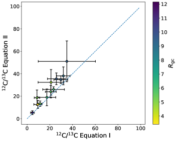
Figure 12: The comparison with $\rm{{}^{12}C/^{13}C}$ results derived by Eq. 30 (Equation I) and Eq. 40 (Equation II). The blue dashed line refers to where the x-value equals the y-value. The color map shows the Galactocentric distances of the targets.

B.4 Different excitation conditions for $\rm{}^{12}CN$ and $\rm{}^{13}CN$

B.4.1 A two $T_{\rm ex}$ layer toy model

In Fig. 2 we show a toy model cloud with two layers having different $T_{\rm ex}$ for the same molecule/transition (e.g., ¹²CN). From the right to the left, there is the background, a layer with a higher $T_{\rm ex}$, a layer with a lower $T_{\rm ex}$, and the observer. Indicatively, we set the high excitation temperature $T_{\rm ex,H}$=30 K and the lower excitation temperature $T_{\rm ex,C}$=10 K. The optical depth of the high $T_{\rm ex}$ layer and the low $T_{\rm ex}$ layer is $\tau_{\rm H}$ and $\tau_{\rm C}$, respectively. The intensity at a certain frequency on the background, on the interface of the two layers, and the intensity observed by us are labeled as $I_{\rm\nu,0}$, $I_{\rm\nu,1}$ and $I_{\rm\nu,2}$, respectively.

We use this toy model in order to explore, in a simple manner, the possible effects of underlying excitation variations (i.e. a non-uniform $T_{\rm ex}$) on the extracted abundance ratios Assuming uniform $T_{\rm ex}$ conditions within each layer the emergent line brightnesses will be (e.g., Mangum & Shirley, 2015):

$$I_{\rm\nu,1}=I_{\rm\nu,0}e^{-\tau_{\rm H}}+B_{\nu}(T_{\rm ex,H})(1-e^{-\tau_{\rm H}})$$ (42)

$$I_{\rm\nu,2}=I_{\nu,1}e^{-\tau_{\rm C}}+B_{\nu}(T_{\rm ex,C})(1-e^{-\tau_{\rm C}})$$ (43)

where $B_{\nu}$ is the Planck function. Here, the spectral line optical depths are strong functions of frequency: $\tau_{\rm H,C}$=$\tau_{0}\,\phi(\nu-\nu_{0})$, with $\phi(\nu-\nu_{0})$ a normalized emission line profile, strongly peaked at some central frequency, and a width determined by the gas motions within each layer. The assumption of a common line profile function $\phi(\nu-\nu_{\circ})=\phi_{\rm C}(\nu-\nu_{0})=\phi_{\rm H}(\nu-\nu_{0})$ for both gas layers is equivalent to the assumption of micro-turbulent and/or thermal gas velocity fields dominating both gas layers. Indeed only under this assumption, the radiative transfer formalism that follows is applicable (with front layer gas able to absorb line radiation emanating from the back layer). Thus we can combine the two previous equations to find:

$$I_{\rm\nu,2}=[I_{\rm\nu,0}e^{-\tau_{\rm H}}+B_{\nu}(T_{\rm ex,H})(1-e^{-\tau_{\rm H}})]e^{-\tau_{\rm C}}+B_{\nu}(T_{\rm ex,C})(1-e^{-\tau_{\rm C}})$$ (44)

In spectroscopic observations, we often measure the line intensity against a non-zero continuum radiation field. This may emanate from the source itself (e.g., dust continuum, synchrotron) and/or from a background source (e.g., the CMB). This (line)-(continuum) differential measurement is obtained spectrally by subtracting the continuum as it is measured at neighbouring frequencies that are not line dominated. If the source itself does not emit any continuum, the subtraction of the OFF-source measurement (as done in single-dish observations) also yields such a (line)-(continuum) differential (with the OFF-line part of such spectrum $\sim$0). The intensity measured then is:

$$\Delta I_{\nu} =I_{\rm\nu,2}-I_{\rm\nu,0}$$ (45)

$$=[I_{\rm\nu,0}e^{-\tau_{\rm H}}+B_{\nu}(T_{\rm ex,H})(1-e^{-\tau_{\rm H}})]e^{-\tau_{\rm C}}$$

$$+B_{\nu}(T_{\rm ex,C})(1-e^{-\tau_{\rm C}})-I_{\rm\nu,0}$$

$$=B_{\nu}(T_{\rm ex,H})(1-e^{-\tau_{\rm H}})e^{-\tau_{\rm C}}+B_{\nu}(T_{\rm ex,C})(1-e^{-\tau_{\rm C}})$$

$$-I_{\rm\nu,0}[1-e^{-(\tau_{\rm H}+\tau_{\rm C})}]$$

Setting the background emission to be a blackbody means $I_{\rm\nu,0}=B_{\nu}(T_{\rm bg})$, and we will have:

$$\Delta I_{\nu} =B_{\nu}(T_{\rm ex,H})(1-e^{-\tau_{\rm H}})e^{-\tau_{\rm C}}+B_{\nu}(T_{\rm ex,C})(1-e^{-\tau_{\rm C}})$$ (46)

$$-B_{\nu}(T_{\rm bg})[1-e^{-(\tau_{\rm H}+\tau_{\rm C})}]$$

where $T_{\rm bg}$ is the background source temperature which here we set to be the CMB temperature ($T_{\rm bg}=T_{\rm CMB}=2.73$ K). Eq. 46 is the same as Eq. 2 in Myers et al. (1996), showing that the two-layer $T_{\rm ex}$ model benefits understanding the line profiles of a collapsing cloud (e.g., Zhou et al., 1993; Myers et al., 1996).

An observer that assumes a uniform $T_{\rm ex}$ single-layer source to analyze its line emission from the two layers, he/she will then assume an effective optical depth and an effective excitation temperature as $\tau_{\rm eff}$ and $T_{\rm ex,eff}$, defined from:

$$\Delta I_{\nu} =[B_{\nu}(T_{\rm ex,eff})-B_{\nu}(T_{\rm bg})](1-e^{-\tau_{\rm eff}})$$ (47)

$$=B_{\nu}(T_{\rm ex,eff})(1-e^{-\tau_{\rm eff}})-B_{\nu}(T_{\rm bg})(1-e^{-\tau_{\rm eff}})$$

From Eq. 46 and Eq. 47, we then have:

$$\tau_{\rm eff}=\tau_{\rm H}+\tau_{\rm C}$$ (48)

and

$$B_{\nu}(T_{\rm ex,eff})\cdot[1-e^{-(\tau_{\rm H}+\tau_{\rm C})}] =B_{\nu}(T_{\rm ex,H})\cdot[e^{-\tau_{\rm C}}-e^{-(\tau_{\rm H}+\tau_{\rm C})}]$$ (49)

$$+B_{\nu}(T_{\rm ex,C})\cdot[e^{-(\tau_{\rm H}+\tau_{\rm C})}-e^{-\tau_{\rm H}}]$$

reordering the Equation above, we obtain:

$$B_{\nu}(T_{\rm ex,eff})=B_{\nu}(T_{\rm ex,H})\cdot a+B_{\nu}(T_{\rm ex,C})\cdot b$$ (50)

$$a=\frac{e^{\tau_{\rm H}}-1}{e^{\tau_{\rm H}+\tau_{\rm C}}-1},\quad b=\frac{e^{\tau_{\rm H}+\tau_{\rm C}}-e^{\tau_{\rm H}}}{e^{\tau_{\rm H}+\tau_{\rm C}}-1}$$ (51)

We can find that $a+b\equiv 1$, it means that the effective $B_{\nu}(T_{\rm ex,eff})$ is actually a weighted-averaged value of $B_{\nu}(T_{\rm ex,H})$ and $B_{\nu}(T_{\rm ex,C})$, with two weighting factors $a$ and $b$. The weighting factors $a$ and $b$ are both functions of $\tau_{\rm H}$ and $\tau_{\rm C}$, which means the effective $T_{\rm ex}$of ¹²CN and ¹³CN emission lines should be different because of their different optical depth.

In Fig. 13 (a), we show the change of $a$ and $b$ with optical depth $\tau$, assuming $\tau_{\rm H}=\tau_{\rm C}=\tau$. The $a$ and $b$ have monotonous and opposite trends to change with $\tau$. The effective temperature of ¹²CN main component will be much lower than the effective temperature of the optically thin ¹³CN main component.

If the linewidth is dominated by macro-turbulence or bulk motion, instead of thermal/micro-turbulence, the two-layer $T_{\rm ex}$ model may not play a dominant role. This might also affect the case in this work, in which the observed linewidths are $\sim 1.5-4\ {\rm km\cdot s^{-1}}$. The radiation between gas layers may not be well-coupled. However, such radiative coupling effects would still bias the isotopic ratios for all methods that need optical-depth corrections.

B.5 The deviation from original assumptions

Deriving $R_{\rm{}^{12}C/^{13}C}$ from CN isotopologues has the basic assumptions including Eq. 35 and Eq. 36. However, considering the different effective $T_{\rm ex}$ between ¹²CN and ¹³CN $N=1\to 0$, and back to Eq. 14 and Eq. 18, we have:

$$R_{\rm 1213} =\frac{N_{\rm main,^{12}CN}}{N_{\rm main,^{13}CN}}$$ (52)

$$=[\frac{{\rm exp}(\frac{E_{\rm u,^{12}CN}}{kT_{\rm ex,^{12}CN}})}{{\rm exp}(\frac{h\nu}{kT_{\rm ex,^{12}CN}})-1}]/[\frac{{\rm exp}(\frac{E_{\rm u,^{13}CN}}{kT_{\rm ex,^{13}CN}})}{{\rm exp}(\frac{h\nu}{kT_{\rm ex,^{13}CN}})-1}]\times\frac{\tau_{\rm m,12}}{\tau_{\rm m,13}}$$

$$=\epsilon_{1}\frac{\tau_{\rm m,12}}{\tau_{\rm m,13}}$$

$$R_{\rm b} =\frac{T_{\rm b,^{12}CN}}{T_{\rm b,^{13}CN}}=\frac{T_{\rm mb,^{12}CN}}{T_{\rm mb,^{13}CN}}$$ (53)

$$=\frac{J_{\nu}(T_{\rm ex,^{12}CN})-J_{\nu}(T_{\rm bg})}{J_{\nu}(T_{\rm ex,^{13}CN})-J_{\nu}(T_{\rm bg})}\times\frac{1-e^{-\tau_{\rm m,12}}}{1-e^{-\tau_{\rm m,13}}}$$

$$=\epsilon_{2}\frac{1-e^{-\tau_{\rm m,12}}}{1-e^{-\tau_{\rm m,13}}}$$

We have assumed that the filling factors $f_{\rm{}^{12}CN}=f_{\rm{}^{13}CN}$ in Eq. 53, so that the brightness temperature ratio equals the main beam temperature ratio. Here we simplify Equations 52 and 53 with $\epsilon_{1}$ and $\epsilon_{2}$:

$$\epsilon_{1}=[\frac{{\rm exp}(\frac{E_{\rm u,^{12}CN}}{kT_{\rm ex,^{12}CN}})}{{\rm exp}(\frac{h\nu}{kT_{\rm ex,^{12}CN}})-1}]/[\frac{{\rm exp}(\frac{E_{\rm u,^{13}CN}}{kT_{\rm ex,^{13}CN}})}{{\rm exp}(\frac{h\nu}{kT_{\rm ex,^{13}CN}})-1}]$$ (54)

$$\epsilon_{2}=\frac{J_{\nu}(T_{\rm ex,^{12}CN})-J_{\nu}(T_{\rm bg})}{J_{\nu}(T_{\rm ex,^{13}CN})-J_{\nu}(T_{\rm bg})}$$ (55)

With our previous assumption that $T_{\rm ex,^{12}CN}=T_{\rm ex,^{13}CN}$, the estimated $R_{\rm 1213}$ and $R_{\rm b}$ are from Eq. 35 and Eq. 36. In this way, $\epsilon_{1}=R^{\rm intrinsic}_{\rm 1213}/R^{\rm estimated}_{\rm 1213}$ and $\epsilon_{2}=R^{\rm intrinsic}_{\rm b}/R^{\rm estimated}_{\rm b}$. We still ignore the difference between other molecular parameters in Eq. 14 of $\rm{}^{12}CN$ and $\rm{}^{13}CN$, except for $E_{\rm u}$ and $T_{\rm ex}$.

Assuming that the column density ratio of ¹²CN and ¹³CN $N=1\to 0$ equals 60, and $\tau_{\rm H}=\tau_{\rm C}=\tau$, we quantify the deviation from the basic assumptions in Eq. 4 and Eq. 5 with the factors $\epsilon_{1}$ and $\epsilon_{2}$ varying with the effective optical depth of ¹²CN $N=1\to 0$ main component $\tau^{\rm main}_{\rm eff}$.

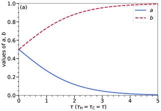
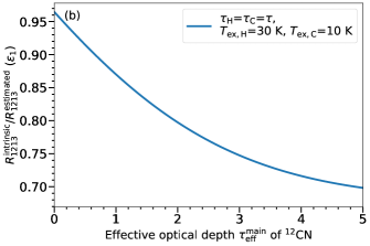
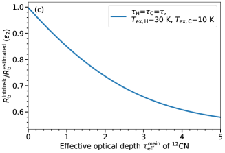
Figure 13: (a). The variation of the weighting factor $a$ (blue solid line) and $b$ (red dashed line) with optical depth. (b). The ratio ($\epsilon_{1}$) between the intrinsic column density ratio and the estimated column density ratio, varying with the effective optical depth of ¹²CN main component ($\tau^{\rm main}_{\rm eff}=\tau_{\rm H}+\tau_{\rm C}$). (c). The ratio ($\epsilon_{2}$) between the intrinsic brightness temperature ratio and the estimated brightness temperature ratio, varying with $\tau^{\rm main}_{\rm eff}$.

In Fig. 13 (b) and (c), we show the change of $\epsilon_{1}$ and $\epsilon_{2}$ as a function of $\tau^{\rm eff}_{\rm main}$. In our toy model with $T_{\rm ex,H}=30$ K and $T_{\rm ex,C}=10$ K, the intrinsic column density ratio will be smaller than the estimated column density ratio. If the optical depth is larger, the discrepancy will be larger. It means using Eq. 4 and Eq. 5 will overestimate the column density ratio and the brightness temperature ratio between ¹²CN and ¹³CN $N=1\to 0$, respectively. When $\tau^{\rm main}_{\rm eff}=\tau_{\rm H}+\tau_{\rm C}\sim 1$, which is similar to the measured optical depth of ¹²CN $N=1\to 0$ main component in our targets, the intrinsic column density ratio will be $\sim$ 15 % lower than the estimated ratio, and the intrinsic brightness temperature ratio will be 10 % lower than the estimated one.

In Fig, 3, we quantify the total effects of these two discrepancies on the derived $R_{\rm{}^{12}C/^{13}C}$. Based on our toy model assumptions and adopting Eq. 4 and Eq. 5, using the HfS fitting method with the ¹²CN main component will let the derived $R_{\rm{}^{12}C/^{13}C}$ $\sim$ 17 % lower than the intrinsic $R_{\rm{}^{12}C/^{13}C}$ when the optical depth of the ¹²CN main component $\sim$ 1. However, if we use the ¹²CN optical-thin satellite line (e.g., $J=3/2\to 1/2$, $F=1/2\to 3/2$ at 113.520 GHz), the derived $R_{\rm{}^{12}C/^{13}C}$ will be closed to the intrinsic column density ratio of ¹²CN and ¹³CN.

B.5.1 More general conditions

The real excitation conditions of a molecular cloud may be much more complex than our toy model. The detailed deviation of the effective optical depth and effective excitation temperature of ¹²CN and ¹³CN is beyond this work. Here we free the values of $T_{\rm ex,^{12}CN}$ and $T_{\rm ex,^{13}CN}$ and analyze the deviation on the $R_{\rm{}^{12}C/^{13}C}$ ratios if the excitation temperature of ¹²CN and ¹³CN $N=1\to 0$ are different.

Considering the $\epsilon 1$ and $\epsilon 2$, Equation 40 should become:

$$\frac{\rm{}^{12}C}{\rm{}^{13}C}=-\frac{R_{13}}{R_{12}}\cdot\frac{\epsilon_{1}\tau_{\rm m,12}}{{\rm ln}[1-\epsilon_{2}\frac{T_{\rm mb,^{13}CN}}{T_{\rm mb,^{12}CN}}(1-e^{-{\tau_{\rm m,12}}})]}$$ (56)

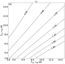
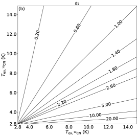
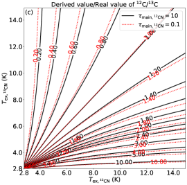
Figure 14: (a). the variation of $\epsilon_{1}$ with $T_{\rm ex}$ of $\rm{}^{12}CN$ and $\rm{}^{13}CN$. (b): the variation of $\epsilon_{2}$ with $T_{\rm ex}$ of $\rm{}^{12}CN$ and $\rm{}^{13}CN$. The contours show the values of $\epsilon_{1}$ and $\epsilon_{2}$ on the upper two figures. (c): assuming the optical depth of the main component of $\rm{}^{12}CN$ ($\tau_{\rm m,^{12}CN}=10$ and $\tau_{\rm m,^{12}CN}=0.1$, respectively), the ratios between the derived $R_{\rm{}^{12}C/^{13}C}$ from Equation 40 and $R_{\rm{}^{12}C/^{13}C}$ from Equation 56. The contours show the value of these ratios.

In Figure 14, we quantify the effect on our derived $R_{\rm{}^{12}C/^{13}C}$ when $T_{\rm ex}$ of $\rm{}^{12}CN$ and $\rm{}^{13}CN$ $N=1\to 0$ are different. Especially, when $T_{\rm ex,^{12}CN}$ is much higher than $T_{\rm ex,^{13}CN}$, $\epsilon_{2}$ will be high and cause a large deviation. The total effect is also sensitive to the difference of $T_{\rm ex,^{12}CN}$ and $T_{\rm ex,^{13}CN}$. The derived $R_{\rm{}^{12}C/^{13}C}$ is not equal to the intrinsic abundance ratio when $T_{\rm ex,^{12}CN}$ equals $T_{\rm ex,^{13}CN}$, because the upper energy levels $E_{\rm u}$ of $\rm{}^{12}CN$ and $\rm{}^{13}CN$ have a slight difference. We ignore it in our $R_{\rm{}^{12}C/^{13}C}$ derivation.

Appendix C Comparison of two HfS fitting procedures

In this section, we test the performances of two procedures that can be used for the HfS fitting. We generate $\rm{}^{12}CN$ $N=1\to 0$ spectra artificially. Then we use the HfS procedure in CLASS and the procedure developed by Estalella (2017) to fit these spectra and test the accuracy and scatter of the results.

We assume the line widths of ¹²CN $N=1\to 0$ components are the same. We also assume that both the intrinsic line and the optical depth $\tau$ have Gaussian profiles. If $\tau=0$, the profiles of the line components can be described as:

$$T_{\rm A}^{\star}(v)=Ae^{-\frac{(v-v_{0})^{2}}{2\sigma^{2}}}$$ (57)

Here $\sigma={\rm FWHM}/2\sqrt{\rm 2ln2}$ and we assume that $\sigma=2\ {\rm km~{}s^{-1}}$. $A$ refers to the intrinsic intensity of a line component, so the total profile can be described as:

$$T_{\rm A}^{\star}(v)=\sum_{k=1}^{n}A_{k}e^{-\frac{(v_{\rm k}-v_{0,k})^{2}}{2\sigma^{2}}}$$ (58)

Here $A_{k}$ indicates the intensities of different line components. We assume $A=5$ K for the main component.

For the line components with the optical depth, we have the following equation:

$$\frac{T^{\star}_{\rm A,hf}}{T^{\star}_{\rm A,m}}=\frac{1-e^{-\tau_{\rm hf}}}{1-e^{-\tau_{\rm m}}}$$ (59)

Here $\tau_{\rm hf}$ and $T^{\star}_{\rm A,hf}$ are the central optical depth and the peak antenna temperature of a certain HfS line component, respectively, while $\tau_{\rm m}$ and $T^{\star}_{\rm A,m}$ refer to the same properties of the main component. Because the difference between the main beam efficiency at the frequency of the main component and the satellite lines is very small (< 0.1% for IRAM 30-m), we replace the $T_{\rm mb}$ in Eq. 8 with the antenna temperature $T^{\star}_{\rm A}$.

We have $\tau_{\rm hf}=R_{\rm hf}*\tau_{\rm m}$. Here, $R_{\rm hf}$ is the column density ratio between an HfS line component and the main component. So line profiles can be described as follows:

$$T_{\rm A}^{\star}(v) =\sum_{k=1}^{n}A(1-e^{-\tau_{\rm hf}\frac{(v_{\rm k}-v_{0,k})^{2}}{2\sigma^{2}}})$$ (60)

$$=\sum_{k=1}^{n}A(1-e^{-R_{\rm hf,k}\tau_{\rm m}\frac{(v_{\rm k}-v_{0,k})^{2}}{2\sigma^{2}}})$$

The basic equation HfS fitting procedures used is  59. With the known $R_{\rm hf}$ and the observed antenna temperature $T^{\star}_{\rm A,hf}$ of multiple HfS line components, the optical depth of the main component ($\tau_{\rm m}$) and $A$ can be derived by the fitting of line profiles. Then we can derive the excitation temperature $T_{\rm ex}$ with Equation 31:

$$T_{\rm ex}=T_{\rm A}(1-e^{-\tau})/(\eta_{\rm mb}f)+T_{\rm bg}$$ (61)

Here we consider $T_{\rm ex}$ in the Rayleigh-Jeans approximation because the procedure in CLASS output $T_{\rm ex}$ under R-J approximation. We use this equation to derive $T_{\rm ex}$ from the procedure of Estalella (2017) in our test.

We generated a list of values ranging from 0 to 5 to be the list of $\tau_{\rm m}$, with an interval at 0.1, to generate ideal $\rm{}^{12}CN$ spectra. There are 500 spectra, which is enough for the test. Figure 15 shows the fitting results of the two procedures and the comparison with ideal values. The procedure from Estalella (2017) has a slightly larger RMS compared with the CLASS procedure, and the accuracy of the $T_{\rm ex}$ is not as good as in CLASS. However, the stability of the procedure from Estalella (2017) is much better than the procedure in CLASS while the results from CLASS include some points that differ a lot from the ideal values. To avoid the risk that the fitting to the real spectra is too bad, we choose the procedure from Estalella (2017) to fit our observed $\rm{}^{12}CN$ $N=1\to 0$ spectra.

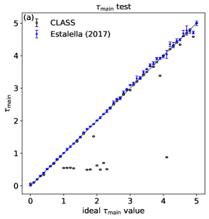
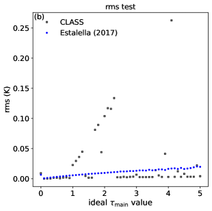
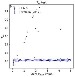
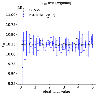
Figure 15: Results for the two HfS fitting procedures. The black hollow squares and solid blue circles show the results from the HfS fitting procedure in CLASS and the procedure developed by  Estalella (2017), respectively. The grey line indicates where the fitted values equal ideal values. (a). The comparison between the ideal $\tau_{\rm m}$ value and the fitting values of the two procedures. The grey line refers to the ideal $\tau_{\rm m}$ we generate. (b). The comparison of the RMS of the fitting to the $\rm{}^{12}CN$ line profile by these two procedures. (c). $T_{\rm ex}$ derived from the two procedures. (d). Same meaning as (c) but zoom in on the y-axis.

Appendix D Spectra of lines

In this section, we show the spectra of the lines we used to derive $R_{\rm{}^{12}C/^{13}C}$ and $R_{\rm{}^{14}N/^{15}N}$. In Fig. 16, we show the $\rm{}^{13}CO$ $J=1\to 0$ lines and the Gaussian fitting to these lines which derives the $V_{\rm LSR}$ of our targets. In Figures  17 and 18 we show the $\rm{}^{12}CN$ and $\rm{}^{13}CN$ $N=1\to 0$ spectra without $\rm{}^{13}CN$ detections. We show the $\rm{}^{12}CN$ and $\rm C^{15}N$ $N=1\to 0$ spectra in Figures 19. The $\rm H^{13}CN$ and $\rm HC^{15}N$ $J=2\to 1$ spectra are shown in Figures 21 and 22. In Figures 23, 24, 25, 26, 27 and 28, we show the HfS fitting results for the detected $\rm{}^{12}CN$.

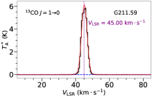
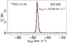
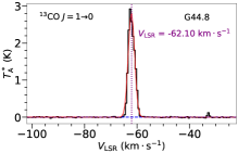
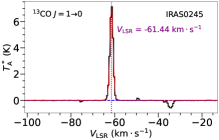
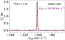
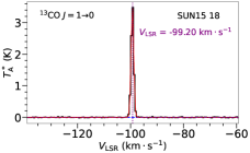
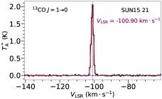
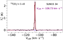
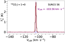
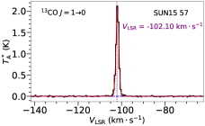
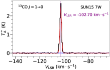
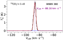
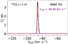
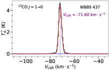
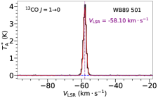
Figure 16: The $\rm{}^{13}CO$ $J=1\to 0$ spectra of our targets. The black steps show the original spectra and the red curves show the Gaussian fitting results. The blue dashed lines show the baseline. The vertical purple dotted lines show the velocity at the local standard rest.

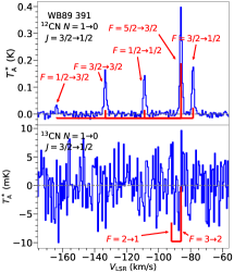
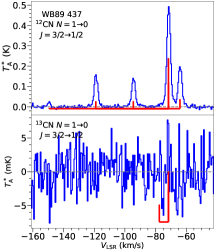
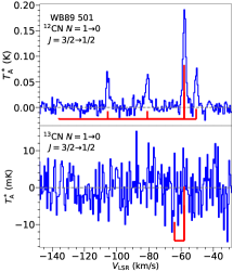
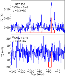
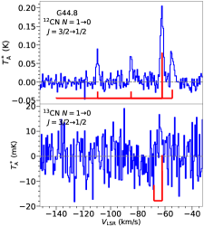
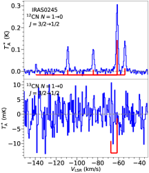
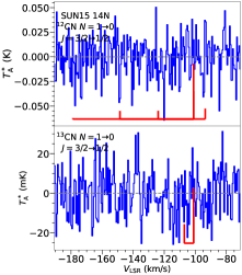
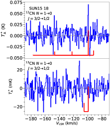
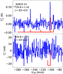
Figure 17: Spectra of ¹²CN and ¹³CN $N=1\to 0$ for targets without ¹³CN (and ¹²CN for some cases) detections.

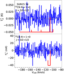
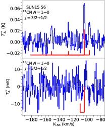
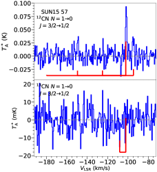
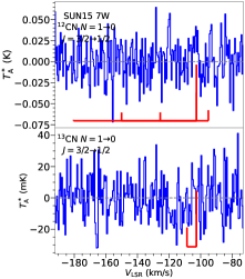
Figure 18: Spectra of ¹²CN and ¹³CN $N=1\to 0$ for targets without ¹³CN (and ¹²CN for some cases) detections. (Continued.).

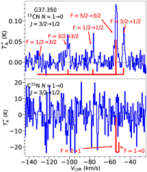
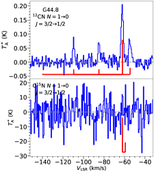
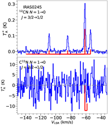
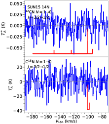
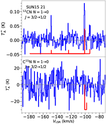
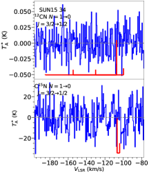
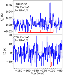
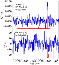
Figure 19: Spectra of ¹²CN and C¹⁵N $N=1\to 0$ for targets without C¹⁵N detections.

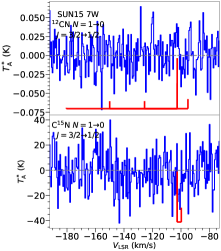
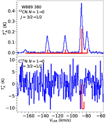
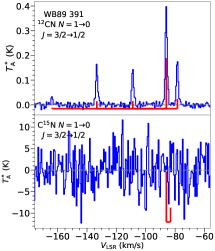
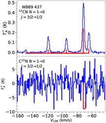
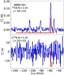
Figure 20: Spectra of ¹²CN and C¹⁵N $N=1\to 0$ for targets without C¹⁵N detections (Continued.).

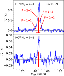
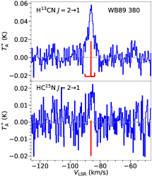
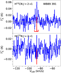
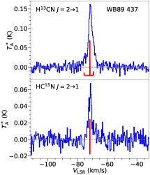
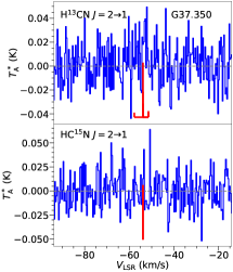
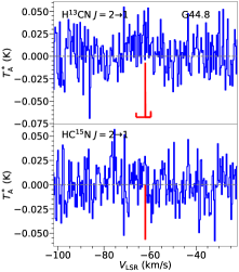
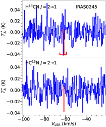
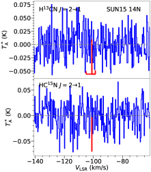
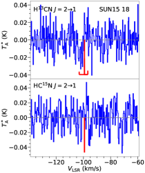
Figure 21: The spectra of $\rm H^{13}CN$ and $\rm HC^{15}N$ at $N=2\to 1$ transition.

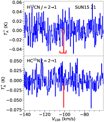
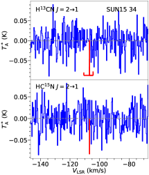
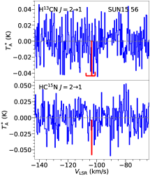
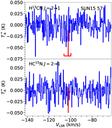
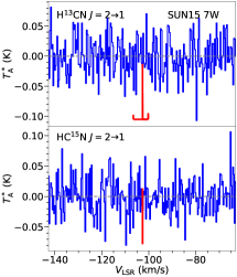
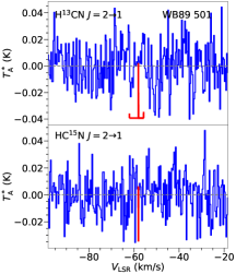
Figure 22: The spectra of $\rm H^{13}CN$ and $\rm HC^{15}N$ at $N=2\to 1$ transition (Continued.).

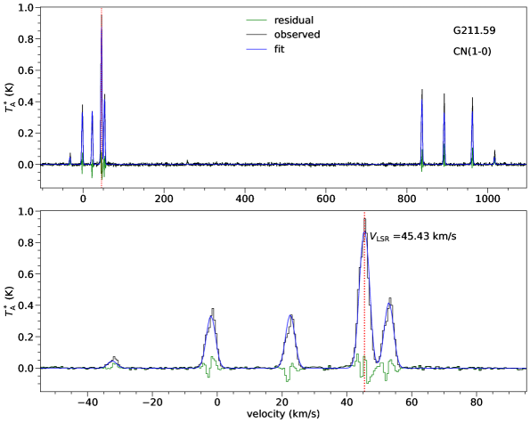
Figure 23: The HfS fitting spectra. The upper panels: the whole spectra of $\rm{}^{12}CN$ $N=1\to 0$ nine components used to do HfS fitting. The lower panels: the zoom-in spectra showing the five components of $\rm{}^{12}CN$ $N=1\to 0\ J=3/2\to 1/2$. The original spectra, HfS fitting results, and residuals are shown in black, blue, and green, respectively. The red dashed lines locate the $V_{\rm LSR}$ of the main component (the HfS fitting results of the other targets are shown below).

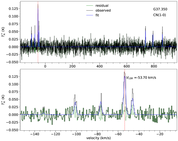
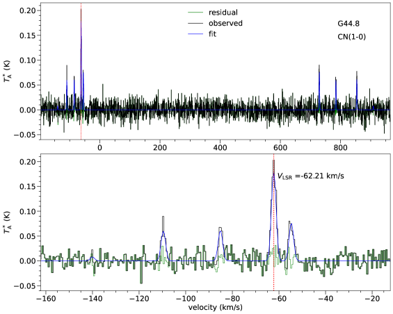
Figure 24: The HfS fitting spectra (Continued.)

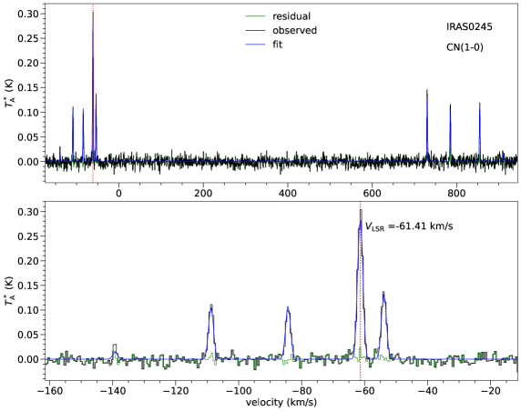
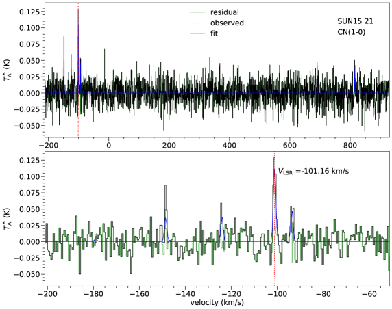
Figure 25: The HfS fitting spectra (Continued.)

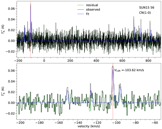
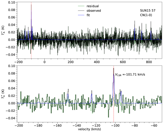
Figure 26: The HfS fitting spectra (Continued.)

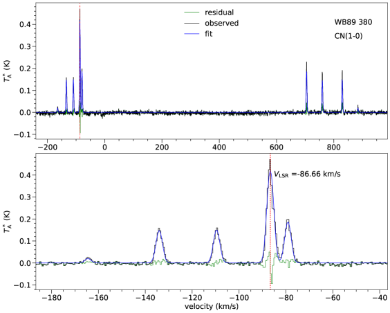
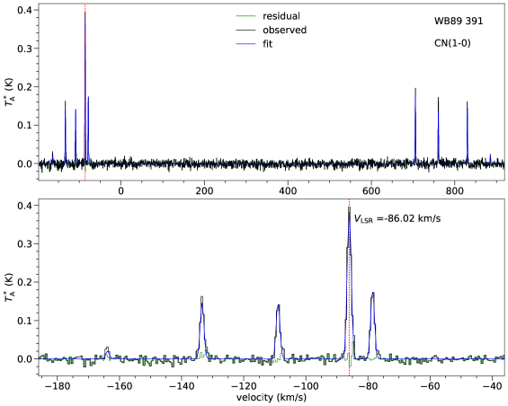
Figure 27: The HfS fitting spectra (Continued.)

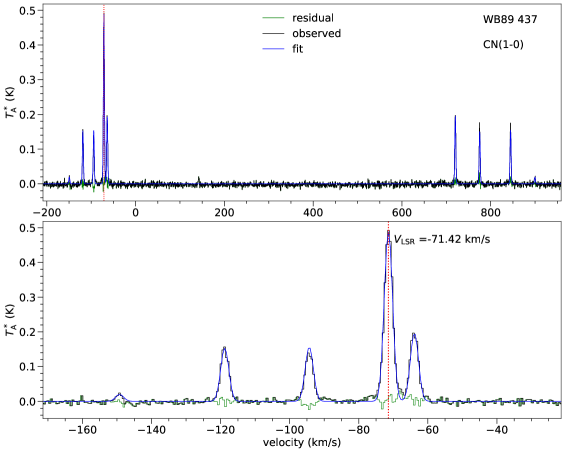
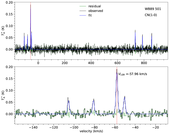
Figure 28: The HfS fitting spectra (Continued.)

Appendix E $\rm{}^{14}N/^{15}N$ derived from HCN isotopologues

For targets with detected $\rm H^{13}CN$ and $\rm HC^{15}N$ $J=2\to 1$ at 2-mm band, the $R_{\rm{}^{14}N/^{15}N}$ can also be derived from their $R_{\rm{}^{12}C/^{13}C}$, as the following equation:

$$\frac{\rm{{}^{14}N}}{\rm{{}^{15}N}}=\frac{I_{\rm H^{13}CN}}{I_{\rm HC^{15}N}}\cdot R_{\rm 12C13C}$$ (62)

Here $I_{\rm H^{13}CN}$ and $I_{\rm HC^{15}N}$ are the integrated intensities of the $\rm H^{13}CN$ and $\rm HC^{15}N$ $J=2\to 1$, respectively. Because the integrated intensity we measured is the integral of antenna temperature and the velocity, we revise the difference between the main beam efficiency at the frequency of $\rm H^{13}CN$ and $\rm HC^{15}N$ $N=1\to 0$. For IRAM 30-m, we have $\eta_{\rm mb,H^{13}CN}=0.687$ and $\eta_{\rm mb,H^{13}CN}=0.688$.

We have detected both $\rm H^{13}CN$ and $\rm HC^{15}N$ $J=2\to 1$ in three targets, two of them have measurements of $R_{\rm{}^{12}C/^{13}C}$ to get $R_{\rm{}^{14}N/^{15}N}$. The line intensities and derived $R_{\rm{}^{14}N/^{15}N}$ from $\rm H^{13}CN$ and $\rm HC^{15}N$ $J=2\to 1$ are shown in Table 8. The spectra of $\rm H^{13}CN$ and $\rm HC^{15}N$ $J=2\to 1$ are shown in Figures 21 and 22.

In Table 8 and Table 9, we show the $R_{\rm{}^{14}N/^{15}N}$ derived from multiplying $R_{\rm{}^{12}C/^{13}C}$ from the $\tau$-correction method and multiplying $R_{\rm{}^{12}C/^{13}C}$ from optically-thin satellite lines, respectively. Adopting $R_{\rm{}^{12}C/^{13}C}$ from the optically-thin satellite line method, the $R_{\rm{}^{14}N/^{15}N}$ value in G211.59 will be $\sim 100$ higher than the one adopting $R_{\rm{}^{12}C/^{13}C}$ from the $\tau$-correction method. For other targets, the change is not significant.

Table 8: $\rm{{}^{14}N/^{15}N}$ ratios derived from HCN isotopologues in our targets (The traditional HfS method).

Sources	$I_{\rm H^{13}CN}$	$I_{\rm HC^{15}N}$	$\rm H^{13}CN/HC^{15}N$	$\rm{}^{14}N/^{15}N$
	($\rm{10^{-2}}$ K $\cdot$ km s -1)	($\rm{10^{-2}}$ K $\cdot$ km s -1)
G211.59	186.1 $\pm$ 4.8	40.0 $\pm$ 4.1	4.7 $\pm$ 0.5	242 $\pm$ 40
G37.350	20.7 $\pm$ 6.3	$\leq$ 14	$\geq$ 1.4	$\geq$ 8.5
G44.8	29.2 $\pm$ 8.0	$\leq$ 17	$\geq$ 1.7	$\geq$ 16
IRAS0245	$\leq$ 144	$\leq$ 10	-	-
SUN15 14N	$\leq$ 241	$\leq$ 15	-	-
SUN15 18	$\leq$ 123	$\leq$ 9.0	-	-
SUN15 21	$\leq$ 191	$\leq$ 12	-	-
SUN15 34	$\leq$ 276	$\leq$ 16	-	-
SUN15 56	$\leq$ 172	$\leq$ 11	-	-
SUN15 57	$\leq$ 174	$\leq$ 11	-	-
SUN15 7W	$\leq$ 298	$\leq$ 17	-	-
WB89 380	34.6 $\pm$ 3.1	6.4 $\pm$ 2.5	5.4 $\pm$ 2.1	329 $\pm$ 171
WB89 391	22.8 $\pm$ 4.1	$\leq$ 7.1	$\geq$ 3.2	$\geq$ 102
WB89 437	89.0 $\pm$ 2.8	24.6 $\pm$ 2.0	3.6 $\pm$ 0.3	$\geq$ 223
WB89 501	$\leq$ 170	$\leq$ 10	-	-

Table 9: $\rm{{}^{14}N/^{15}N}$ ratios from HCN isotopologues with $\rm{}^{12}C/^{13}C$ from $\rm{}^{12}CN$ satellite lines in our targets.

Sources	$\rm H^{13}CN/HC^{15}N$	$\rm{}^{12}C/^{13}C$	$\rm{}^{14}N/^{15}N$
G211.59	4.7 $\pm$ 0.5	71.7 $\pm$ 9.5	336 $\pm$ 57
WB89 380	5.4 $\pm$ 2.1	57 $\pm$ 13	312 $\pm$ 141
WB89 391	$\geq$ 3.2	$\geq$ 36	$\geq$ 121
WB89 437	3.6 $\pm$ 0.3	$\geq$ 59	$\geq$ 211

Appendix F The linear fitting functions of Galactic $R_{\rm{}^{12}C/^{13}C}$ and $R_{\rm{}^{14}N/^{15}N}$ gradients

We use the Markov Chain Monte Carlo procedures to fit linear functions for the measurements shown in Fig. 7 (b) and Fig. 6 (b), respectively. The linear fitting function of the Galactic $R_{\rm{}^{12}C/^{13}C}$ ratio is:

$${\rm{}^{12}C/^{13}C}=4.08\,(^{+0.86}_{-0.43})R_{\rm gc}+18.8\,(^{+2.6}_{-6.6})$$ (63)

The linear fitting function of the Galactic $R_{\rm{}^{14}N/^{15}N}$ gradient is:

$${\rm{}^{14}N/^{15}N}=10.6\,(^{+5.6}_{-8.8})R_{\rm gc}+96\,(^{+61}_{-44})$$ (64)

Here, $R_{\rm gc}$ is the Galactocentric distance in the unit of kpc. However, it is highly risky to read a fitted value of $R_{\rm{}^{12}C/^{13}C}$ or $R_{\rm{}^{14}N/^{15}N}$ from these gradients. These gradients suffer large scatters, possibly because of the inhomogeneous mixing, the non-LTE conditions, and the astrochemistry of individual targets. The Galactic chemical evolution models predict that both $R_{\rm{}^{12}C/^{13}C}$ and $R_{\rm{}^{14}N/^{15}N}$ gradients are non-linear curves (e.g., Romano et al., 2017, 2019). For these reasons, we highly recommend using the direct measurements of $R_{\rm{}^{12}C/^{13}C}$ and $R_{\rm{}^{14}N/^{15}N}$ of individual targets, instead of values fitted from curves.

Appendix G The Figure of Galactic H II regions

In Fig 29, we compare the locations of H II regions in Arellano-Córdova et al. (2020) and the locations of ISM targets for Galactic $R_{\rm{}^{12}C/^{13}C}$ gradient on the Galactic plane. We find that most of the ISM targets are located in the same quadrants as those H II regions. It indicates the element abundance may be similarly well-mixed in the ISM targets compared to the mixed condition in those H II regions.

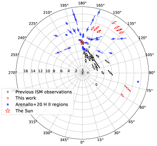
Figure 29: The location of ISM targets in isotopic ratio works and H II regions in the Galactic plane. The pole is the Galactic center and the big red star shows the location of the Sun. The black dots represent the locations of targets in previous works (Savage et al., 2002; Milam et al., 2005; Langer & Penzias, 1990; Wouterloot & Brand, 1996; Giannetti et al., 2014; Jacob et al., 2020) and the red squares represent the targets in this work. The blue stars represent the location of H II regions in Arellano-Córdova et al. (2020).

References

- Adande & Ziurys (2012) Adande G. R., Ziurys L. M., 2012, ApJ, 744, 194
- Arellano-Córdova et al. (2020) Arellano-Córdova K. Z., Esteban C., García-Rojas J., Méndez-Delgado J. E., 2020, MNRAS, 496, 1051
- Audouze et al. (1973) Audouze J., Truran J. W., Zimmerman B. A., 1973, ApJ, 184, 493
- Ayres et al. (2013) Ayres T. R., Lyons J. R., Ludwig H. G., Caffau E., Wedemeyer-Böhm S., 2013, ApJ, 765, 46
- Bachiller et al. (1997) Bachiller R., Fuente A., Bujarrabal V., Colomer F., Loup C., Omont A., de Jong T., 1997, A&A, 319, 235
- Bogey et al. (1984) Bogey M., Demuynck C., Destombes J. L., 1984, Canadian Journal of Physics, 62, 1248
- Botelho et al. (2020) Botelho R. B., Milone A. d. C., Meléndez J., Alves-Brito A., Spina L., Bean J. L., 2020, MNRAS, 499, 2196
- Brand & Blitz (1993) Brand J., Blitz L., 1993, A&A, 275, 67
- Brand & Wouterloot (1995) Brand J., Wouterloot J. G. A., 1995, A&A, 303, 851
- Brand et al. (1986) Brand J., Blitz L., Wouterloot J. G. A., 1986, A&AS, 65, 537
- Brand et al. (1988) Brand J., Blitz L., Wouterloot J., 1988, in Blitz L., Lockman F. J., eds, , Vol. 306, The Outer Galaxy. p. 40, doi:10.1007/3-540-19484-3_4
- Burbidge et al. (1957) Burbidge E. M., Burbidge G. R., Fowler W. A., Hoyle F., 1957, Reviews of Modern Physics, 29, 547
- Chen et al. (2021) Chen J. L., et al., 2021, ApJS, 257, 39
- Colzi et al. (2018) Colzi L., Fontani F., Caselli P., Ceccarelli C., Hily-Blant P., Bizzocchi L., 2018, A&A, 609, A129
- Colzi et al. (2020) Colzi L., Sipilä O., Roueff E., Caselli P., Fontani F., 2020, A&A, 640, A51
- Colzi et al. (2022) Colzi L., et al., 2022, CHEMOUT: CHEMical complexity in star-forming regions of the OUTer Galaxy III. Nitrogen isotopic ratios in the outer Galaxy, doi:10.48550/ARXIV.2209.10620, https://arxiv.org/abs/2209.10620
- Cristallo et al. (2009) Cristallo S., Straniero O., Gallino R., Piersanti L., Domínguez I., Lederer M. T., 2009, ApJ, 696, 797
- Cristallo et al. (2015) Cristallo S., Straniero O., Piersanti L., Gobrecht D., 2015, ApJS, 219, 40
- Enokiya et al. (2021) Enokiya R., et al., 2021, PASJ, 73, S256
- Estalella (2017) Estalella R., 2017, PASP, 129, 025003
- Esteban et al. (2022) Esteban C., Méndez-Delgado J. E., García-Rojas J., Arellano-Córdova K. Z., 2022, ApJ, 931, 92
- Falgarone et al. (1998) Falgarone E., Panis J. F., Heithausen A., Perault M., Stutzki J., Puget J. L., Bensch F., 1998, A&A, 331, 669
- Feng et al. (2020) Feng S., et al., 2020, ApJ, 901, 145
- Foreman-Mackey et al. (2013) Foreman-Mackey D., Hogg D. W., Lang D., Goodman J., 2013, PASP, 125, 306
- Fu et al. (2022) Fu X., et al., 2022, A&A, 668, A4
- Giannetti et al. (2014) Giannetti A., et al., 2014, A&A, 570, A65
- Goldsmith & Langer (1999) Goldsmith P. F., Langer W. D., 1999, ApJ, 517, 209
- Goodman & Weare (2010) Goodman J., Weare J., 2010, Communications in Applied Mathematics and Computational Science, 5, 65
- Greve et al. (2009) Greve T. R., Papadopoulos P. P., Gao Y., Radford S. J. E., 2009, ApJ, 692, 1432
- Guilloteau & Lucas (2000) Guilloteau S., Lucas R., 2000, in Mangum J. G., Radford S. J. E., eds, Astronomical Society of the Pacific Conference Series Vol. 217, Imaging at Radio through Submillimeter Wavelengths. p. 299
- Henkel & Mauersberger (1993) Henkel C., Mauersberger R., 1993, A&A, 274, 730
- Henkel et al. (1982) Henkel C., Wilson T. L., Bieging J., 1982, A&A, 109, 344
- Henkel et al. (1985) Henkel C., Guesten R., Gardner F. F., 1985, A&A, 143, 148
- Henkel et al. (1993) Henkel C., Mauersberger R., Wiklind T., Huettemeister S., Lemme C., Millar T. J., 1993, A&A, 268, L17
- Henkel et al. (1998) Henkel C., Chin Y. N., Mauersberger R., Whiteoak J. B., 1998, A&A, 329, 443
- Henkel et al. (2014) Henkel C., et al., 2014, A&A, 565, A3
- Hily-Blant et al. (2010) Hily-Blant P., Walmsley M., Pineau Des Forêts G., Flower D., 2010, A&A, 513, A41
- Jacob et al. (2020) Jacob A. M., Menten K. M., Wiesemeyer H., Güsten R., Wyrowski F., Klein B., 2020, A&A, 640, A125
- Kaiser et al. (1991) Kaiser M. E., Hawkins I., Wright E. L., 1991, ApJ, 379, 267
- Karakas & Lattanzio (2014) Karakas A. I., Lattanzio J. C., 2014, Publ. Astron. Soc. Australia, 31, e030
- Kutner & Ulich (1981) Kutner M. L., Ulich B. L., 1981, ApJ, 250, 341
- Langer & Penzias (1990) Langer W. D., Penzias A. A., 1990, ApJ, 357, 477
- Langer & Penzias (1993) Langer W. D., Penzias A. A., 1993, ApJ, 408, 539
- Langer et al. (1984) Langer W. D., Graedel T. E., Frerking M. A., Armentrout P. B., 1984, ApJ, 277, 581
- Li et al. (2016) Li H.-K., Zhang J.-S., Liu Z.-W., Lu D.-R., Wang M., Wang J., 2016, Research in Astronomy and Astrophysics, 16, 47
- Limongi & Chieffi (2018) Limongi M., Chieffi A., 2018, ApJS, 237, 13
- Loison et al. (2020) Loison J.-C., Wakelam V., Gratier P., Hickson K. M., 2020, MNRAS, 498, 4663
- Mangum & Shirley (2015) Mangum J. G., Shirley Y. L., 2015, PASP, 127, 266
- Marigo (2001) Marigo P., 2001, A&A, 370, 194
- Marty et al. (2011) Marty B., Chaussidon M., Wiens R. C., Jurewicz A. J. G., Burnett D. S., 2011, Science, 332, 1533
- Matteucci & D’Antona (1991) Matteucci F., D’Antona F., 1991, A&A, 247, L37
- McNamara et al. (2000) McNamara D. H., Madsen J. B., Barnes J., Ericksen B. F., 2000, PASP, 112, 202
- Méndez-Delgado et al. (2022) Méndez-Delgado J. E., Amayo A., Arellano-Córdova K. Z., Esteban C., García-Rojas J., Carigi L., Delgado-Inglada G., 2022, MNRAS, 510, 4436
- Meyer (1994) Meyer B. S., 1994, ARA&A, 32, 153
- Meynet & Maeder (2002a) Meynet G., Maeder A., 2002a, A&A, 381, L25
- Meynet & Maeder (2002b) Meynet G., Maeder A., 2002b, A&A, 390, 561
- Milam (2007) Milam S. N., 2007, Following carbon’s evolutionary path: From nucleosynthesis to the solar system. The University of Arizona
- Milam et al. (2005) Milam S. N., Savage C., Brewster M. A., Ziurys L. M., Wyckoff S., 2005, ApJ, 634, 1126
- Myers et al. (1996) Myers P. C., Mardones D., Tafalla M., Williams J. P., Wilner D. J., 1996, ApJ, 465, L133
- Nakagawa (1980) Nakagawa N., 1980, Interstellar Molecules, 87, 365
- Nomoto et al. (2013) Nomoto K., Kobayashi C., Tominaga N., 2013, ARA&A, 51, 457
- Pettini et al. (2002) Pettini M., Ellison S. L., Bergeron J., Petitjean P., 2002, A&A, 391, 21
- Pignatari et al. (2015) Pignatari M., et al., 2015, ApJ, 808, L43
- Reid et al. (2014) Reid M. J., et al., 2014, ApJ, 783, 130
- Reid et al. (2016) Reid M. J., Dame T. M., Menten K. M., Brunthaler A., 2016, ApJ, 823, 77
- Reid et al. (2019) Reid M. J., et al., 2019, ApJ, 885, 131
- Richardson et al. (1986) Richardson K. J., White G. J., Phillips J. P., Avery L. W., 1986, MNRAS, 219, 167
- Ritchey et al. (2011) Ritchey A. M., Federman S. R., Lambert D. L., 2011, ApJ, 728, 36
- Röllig & Ossenkopf (2013) Röllig M., Ossenkopf V., 2013, A&A, 550, A56
- Romano (2022) Romano D., 2022, A&ARv, 30, 7
- Romano & Matteucci (2003) Romano D., Matteucci F., 2003, MNRAS, 342, 185
- Romano et al. (2017) Romano D., Matteucci F., Zhang Z. Y., Papadopoulos P. P., Ivison R. J., 2017, MNRAS, 470, 401
- Romano et al. (2019) Romano D., Matteucci F., Zhang Z.-Y., Ivison R. J., Ventura P., 2019, MNRAS, 490, 2838
- Roueff et al. (2015) Roueff E., Loison J. C., Hickson K. M., 2015, A&A, 576, A99
- Saleck et al. (1994) Saleck A. H., Simon R., Winnewisser G., 1994, ApJ, 436, 176
- Sandell & Wright (2010) Sandell G., Wright M., 2010, ApJ, 715, 919
- Savage et al. (2002) Savage C., Apponi A. J., Ziurys L. M., Wyckoff S., 2002, ApJ, 578, 211
- Savva et al. (2003) Savva D., Little L. T., Phillips R. R., Gibb A. G., 2003, MNRAS, 343, 259
- Skatrud et al. (1983) Skatrud D. D., De Lucia F. C., Blake G. A., Sastry K. V. L. N., 1983, Journal of Molecular Spectroscopy, 99, 35
- Smith & Adams (1980) Smith D., Adams N. G., 1980, ApJ, 242, 424
- Sun et al. (2015) Sun Y., Xu Y., Yang J., Li F.-C., Du X.-Y., Zhang S.-B., Zhou X., 2015, ApJ, 798, L27
- Sun et al. (2017) Sun Y., Su Y., Zhang S.-B., Xu Y., Chen X.-P., Yang J., Jiang Z.-B., Fang M., 2017, ApJS, 230, 17
- Tafalla et al. (2002) Tafalla M., Myers P. C., Caselli P., Walmsley C. M., Comito C., 2002, ApJ, 569, 815
- Tang et al. (2019) Tang X. D., et al., 2019, A&A, 629, A6
- Timmes et al. (1995) Timmes F. X., Woosley S. E., Weaver T. A., 1995, ApJS, 98, 617
- Watson et al. (1976) Watson W. D., Anicich V. G., Huntress W. T. J., 1976, ApJ, 205, L165
- Wiescher et al. (2010) Wiescher M., Görres J., Uberseder E., Imbriani G., Pignatari M., 2010, Annual Review of Nuclear and Particle Science, 60, 381
- Willacy et al. (1998) Willacy K., Langer W. D., Velusamy T., 1998, ApJ, 507, L171
- Wilson & Rood (1994) Wilson T. L., Rood R., 1994, ARA&A, 32, 191
- Wilson et al. (2013) Wilson T. L., Rohlfs K., Hüttemeister S., 2013, Tools of Radio Astronomy, doi:10.1007/978-3-642-39950-3.
- Woosley & Weaver (1995) Woosley S. E., Weaver T. A., 1995, ApJS, 101, 181
- Wouterloot & Brand (1989) Wouterloot J. G. A., Brand J., 1989, A&AS, 80, 149
- Wouterloot & Brand (1996) Wouterloot J. G. A., Brand J., 1996, A&AS, 119, 439
- Wouterloot et al. (2008) Wouterloot J. G. A., Henkel C., Brand J., Davis G. R., 2008, A&A, 487, 237
- Wu et al. (2010) Wu J., Evans Neal J. I., Shirley Y. L., Knez C., 2010, ApJS, 188, 313
- Yan et al. (2019) Yan Y. T., et al., 2019, ApJ, 877, 154
- Yan et al. (2023) Yan Y. T., et al., 2023, A&A, 670, A98
- Zhang et al. (2016) Zhang Z.-Y., Papadopoulos P. P., Ivison R. J., Galametz M., Smith M. W. L., Xilouris E. M., 2016, Royal Society Open Science, 3, 160025
- Zhang et al. (2020) Zhang J. S., et al., 2020, ApJS, 249, 6
- Zhang et al. (2021) Zhang Y., Snellen I. A. G., Mollière P., 2021, A&A, 656, A76
- Zhou et al. (1993) Zhou S., Evans Neal J. I., Koempe C., Walmsley C. M., 1993, ApJ, 404, 232
- van Dishoeck & Black (1988) van Dishoeck E. F., Black J. H., 1988, ApJ, 334, 771