Clustered Policy Decision Ranking

Abstract

Policies trained via reinforcement learning (RL) are often very complex even for simple tasks. In an episode with n time steps, a policy will make n decisions on actions to take, many of which may appear non-intuitive to the observer. Moreover, it is not clear which of these decisions directly contribute towards achieving the reward and how significant their contribution is. Given a trained policy, we propose a black-box method based on statistical covariance estimation that clusters the states of the environment and ranks each cluster according to the importance of decisions made in its states. We compare our measure against a previous statistical fault localization based ranking procedure.

Introduction

Reinforcement learning is a powerful method for training policies that complete tasks in complex environments via sequential action selection (Sutton and Barto 2018). The policies produced are optimized to maximize the expected cumulative reward provided by the environment. While reward maximization is clearly an important goal, this single measure may not reflect other objectives that an engineer or scientist may desire in training RL agents. Focusing solely on performance risks overlooking the demand for models that are easier to analyse, predict and interpret (Lewis, Li, and Sycara 2020). Our hypothesis is that many trained policies are needlessly complex, i.e., that there exist alternative policies that perform just as well or nearly as well but that are significantly simpler.

The starting point for our definition of simplicity is the assumption that there exists a way to make a simpler choice based on repeating the most recent action taken. We argue that this may be the case for many environments in which RL is applied. That is, there may be states or clusters of states in which the most recent action can be repeated without a drastic drop in expected reward obtained. The tension between performance and simplicity is central to the field of explainable AI (XAI), and machine learning as a whole (Gunning and Aha 2019).

Ranking policy decisions according to their importance was introduced by (Pouget et al. 2021), who use spectrum-based fault localization (SBFL) techniques to approximate the contribution of decisions to reward attainment. This approach constitutes a statistical ranking of individual states.

We theorize however that a single state cannot have particularly notable importance, especially in more complex environments. As discussed in (McNamee and Chockler 2022), another exploration of policy simplification, previous work treats actions independently, whereas it is often the case that action sequences, or even non-contiguous combinations of actions, may synergize to have a large effect on reward acquisition (Sutton, Precup, and Singh 1999). Extending SBFL-based and causality-based policy ranking into the multi-action domain may result in qualitatively distinct policy ranking results compared to single-action methods.

The key contribution of this paper is a novel method for clustering policy decisions according to their co-variable correlation with significant impact on the attainment of the goal, and subsequent ranking of those clusters. We argue that the clustered decisions grant insight into the operation of the policy, and that this clustered ranking method describes the importance of states more accurately than an individual statistical ranking. We evaluate our clustering method by using the clusters to simplify policies without compromising performance, hence addressing one of the main hurdles for wide adoption of deep RL: the high complexity of trained policies.

We use the same proxy measure for evaluating the quality of our ranking as (Pouget et al. 2021): we construct new, simpler policies (“pruned policies”) that only use the top-ranked clusters, without retraining, and compare the reward achieved by these policies to the original policy’s reward.

Our experiments with agents for MiniGrid (Chevalier Boisvert, Willems, and Pal 2018) and environments from Atari Zoo (Brockman et al. 2016) including Bowling, Krull, and Hero demonstrate that pruned policies can maintain high performance and also that performance monotonically approaches that of the original policy as more highly ranked decisions are included from the original policy. As pruned policies are much easier to understand than the original policies, we consider this a potentially useful method in the context of explainable RL. As pruning a given policy does not require re-training, the procedure is relatively lightweight. Furthermore, the clustering of states itself provides an important insight into the relationships of particular decisions to the performance of the policy overall.

The code for the experiments and full experimental results are available at https://anonymous.4open.science/r/Clustered-Policy-Decision-Ranking.

Background

Reinforcement Learning

We use a standard reinforcement learning (RL) setup and assume that the reader is familiar with the basic concepts. An environment in RL is defined as a Markov decision process (MDP) with components $\left\{S,A,P,R,\gamma\right\}$, where $S$ is the set of states $s$, $A$ is the set of actions $a$, $P$ is the transition function, $R$ is the reward function, and $\gamma$ is the discount factor. An agent seeks to learn a policy $\pi:S\rightarrow A$ that maximizes the total discounted reward. Starting from the initial state $s_{0}$ and given the policy $\pi$, the state-value function is the expected future discounted reward as follows:

$$V_{\pi}(s_{0})=\mathbb{E}\left(\sum_{t=0}^{\infty}\gamma^{t}R(s_{t},\pi(s_{t}),s_{t+1})\right).$$ (1)

A policy $\pi:S\rightarrow A$ maps states to the actions taken in these states and may be stochastic. We treat the policy as a black box, and hence make no further assumptions about $\pi$.

Mutation

When we simplify a policy, we mutate some of its states such that the default action (repeating the previous action) is taken rather than the policy action. Given a state space S, a simplified policy has a ”mutated” space $S_{M}\subset S$ and a mutually exclusive ”normal” space $S_{N}\subset S$, such that any time a state is encountered in $S_{N}$ the policy action is taken and any time a state is encountered in $S_{M}$ the default action is taken.

TF-IDF Vectorization

TF-IDF, which stands for Term Frequency-Inverse Document Frequency, is a numerical statistic used in information retrieval and text mining to evaluate the importance of a word in a document relative to a collection of documents (corpus). The goal of TF-IDF is to quantify the significance of a term within a document by considering both its frequency within the document (TF) and its rarity across the entire corpus (IDF) (Jones 1972).

Given a corpus $C$, document $D$ and term $t$, we define $C(t)$ to be the number of documents containing $t$, and $D(t)$ to be the number of appearances of $t$ in $D$. The TF-IDF score of a term $t$ in document $D$ is calculated as follows.

$$\mbox{TF}(D,t)=D(t)/|D|$$ (2)

$$\mbox{IDF}(t)=\log(|C|/(C(t)+1))$$ (3)

$$\mbox{TF-IDF}(D,t)=TF(D,t)*IDF(t)$$ (4)

Each document $D$ is then represented as a vector with the entry corresponding to each term $t$ in the corpus being $\mbox{TF-IDF}(D,t)$. The resulting vectorized documents provide a way to identify the importance of terms within a document in the context of a larger corpus. It is commonly used in various natural language processing (NLP) tasks such as document retrieval, text classification, and information retrieval. Terms with higher TF-IDF scores are considered more significant to a particular document.

Principle Component Analysis

Principal Component Analysis (PCA) (Hotelling 1936) is a dimensionality reduction technique widely used in statistics and machine learning. Its primary goal is to transform high-dimensional data into a new coordinate system, where the axes (principal components) are ranked by their importance in explaining the variance in the data. The first principal component captures the most significant variance, the second principal component (orthogonal to the first) captures the second most significant variance, and so on.

PCA starts by computing the covariance matrix of the standardized data. The covariance matrix summarizes the relationships between different features, indicating how they vary together. The next step involves finding the eigenvalues and corresponding eigenvectors of the covariance matrix. The eigenvectors represent the principal components and are listed in order of decreasing variance. By selecting a subset of these principal components with the highest variance, you can achieve dimensionality reduction while retaining the most important information in the data.

Method

Random Sampling

Algorithm 1 Sample Trajectory

Input: $\mu$, $\tau$, env, policy, default
Output: $S_{M}$ or $S_{N}$, averageReward

1:Let $S_{M}$, $S_{N}$ = {}

2:Let totalReward = 0

3:for _ in range($\tau$) do

4:     env.reset()

5:     while not env.end() do

6:         Let state = env.getEncodedState()

7:         if state $\in S_{M}$ then

8:              env.step(default)

9:         else if state $\in S_{N}$ then

10:              env.step(policy)

11:         else if random() $<\mu$ then

12:              $S_{M}$.add(state)

13:              env.step(default)

14:         else

15:              $S_{N}$.add(state)

16:              env.step(policy)

17:         end if

18:         totalReward += env.reward()

19:     end while

20:end for

21:if $\mu<0.5$ then return $S_{M}$, totalReward$/\tau$

22:else  return $S_{N}$, totalReward$/\tau$

23:end if

The naive approach to finding optimal clusters would be to create a suite of all potential sets $S_{N}$ and determining the consequent trajectory with the highest reward, but for obvious reasons this is not practical. The set of all potential $S_{N}$ is $2^{S}$ (powerset of S), so instead we randomly sample trajectories. In order to generate a randomly sampled suite of $S_{N}$ sets, we define a mutation rate hyper-parameter $\mu$, a suite size hyper-parameter N, and a trials hyper-paremeter $\tau$, and perform N runs of Alg. 1. We may also employ an encoder that simplifies our state space to a set of abstract states, thereby decreasing the size of S and thus the search space for sets $S_{N}$. This encoder may for example include down-scaling or grey-scaling images that are input to the agent, or discretizing a continuous state space. The more the encoder simplifies the environment without losing important information, the better and faster this process performs.

We define a “+” suite as a suite with a $\mu>0.5$. For such suites, we record the sets $S_{N}$ corresponding to successful runs as defined by some condition unique to the environment and their average rewards. We define a “-” suite as a suite with $\mu<0.5$. For such suites, we record the sets $S_{M}$ corresponding to unsuccessful runs and their average rewards. For any run, we generate a “+” suite and a “-” suite, each of size N, using mutation rates $\mu$ and $1-\mu$. The recorded sets in each form the two types of important sets, those that significantly increase reward by being restored, and those that significantly decrease reward by being mutated.

Vectorization

We employ a modified version of the TF-IDF process to vectorize our randomly sampled suites. $C$ now refers to a randomly sampled suite, $D$ now refers to a cluster from that suite and $t$ to a state in the environment. $R(D)$ refers to the reward achieved by cluster $D$ min-max normalized across suite $C$. $T(C)$ refers to 1 for the “-” suite and 0 for the “+” suite. Each state can only appear once in a cluster, so $D(t)$ is now 1 if $t\in D$ and 0 otherwise. We modify Eq. 2 as follows.

$$\mbox{TF}(D,t)=C(t)*R(D)^{2}-T(C)$$ (5)

Typical IDF makes it so that terms that appear often across documents have very low scores. In fact, a term that is in every document would receive an IDF of 0. For our purposes these states should be down-weighted, but not to such a high degree. We define a downweighting hyper-parameter $\delta$ and modify Eq. 3 as follows.

$$\mbox{IDF}(t_{k})=(\log_{\delta}(C(t_{k})+\delta))^{-1}.$$ (6)

We leave Eq. 4 unchanged. By vectorizing using TF-IDF scores in the same way as described above, we now have two collections of vectorized clusters where important states will be represented by large positive or negative scores and states that were important together will have such large scores together across vectors.

Cluster Extraction

We would like to extract small clusters that appear together often in these high scoring vectors. We can create three matrices: The “-” matrix has the vectorizations of the “-” suite for its columns, the “+” matrix has the vectorizations of the “+” suite for its columns, and the “+-” matrix has the vectorizations of both suites for its columns.

By applying the PCA algorithm to each of our three matrices we can get the principle components, each a linear combination of our states. Here, we define two more hyper-parameters: $\sigma$ is the number of clusters we extract, and $\eta$ is the proportion of states in a component to cluster. For each of the first $\sigma$ principle components of highest order, we extract a cluster consisting of the $\eta*|S|$ states with corresponding coefficients of the greatest absolute value in that component. Thus for each matrix we get $\sigma$ clusters each with $\eta*|S|$ states. For each cluster, we then execute runs of the policy pruned to where only states in that cluster are not mutated and record the average reward achieved. The clusters are ranked in order of decreasing average reward.

Experimental Results

Experimental Setup

We present the results of our experiments on a number of standard benchmarks. The first benchmark is Minigrid (Chevalier Boisvert, Willems, and Pal 2018), a gridworld in which the agent operates with a cone of vision and can navigate many different grids, making it more complex than a standard gridworld. In each step the agent can turn or move forward.

The second set of experiments was performed on Atari games (Brockman et al. 2016). We use policies that are trained using third-party code. No state abstraction is applied to the gridworld environments. For the Atari games, as is typically done, we crop the game’s border, grey-scale, down-sample to 18×14, and lower the precision of pixel intensities to make the enormous state space manageable. Note that these abstractions are not a contribution of ours, and were primarily chosen for their simplicity. For our main experiments, we use “repeat previous action” as the default action. As a baseline, we compare our clustering method to the pre-existing processes to accomplish policy pruning, those being the SBFL, FreqVis, and Rand rankings explored in (Pouget et al. 2021).

We use the performance of pruned policies as a proxy for the quality of the ranking computed by our algorithm. In pruned policies, all but the top-ranked states are mutated. The pruned policies for SBFL, FreqVis, and Rand are designed as specified in  (Pouget et al. 2021). Beginning with all states mutated, an increasing fraction of states are restored in each subsequent pruned policy, in order of decreasing rank.

Similarly, for each of our rankings “cluster+”, “cluster-”, and “cluster+-” we first run with all states mutated, and “restore” (i.e., return to the original) another cluster in each pruned policy in order of decreasing cluster rank. We then have two metrics by which to compare ranking processes. The first is what percent of the original reward can be restored given the proportion of the state space that is restored according to that process. The second is what percent of the original reward can be restored given what proportion of the actions taken in a trajectory are policy actions rather than default actions according to that process.

Performance

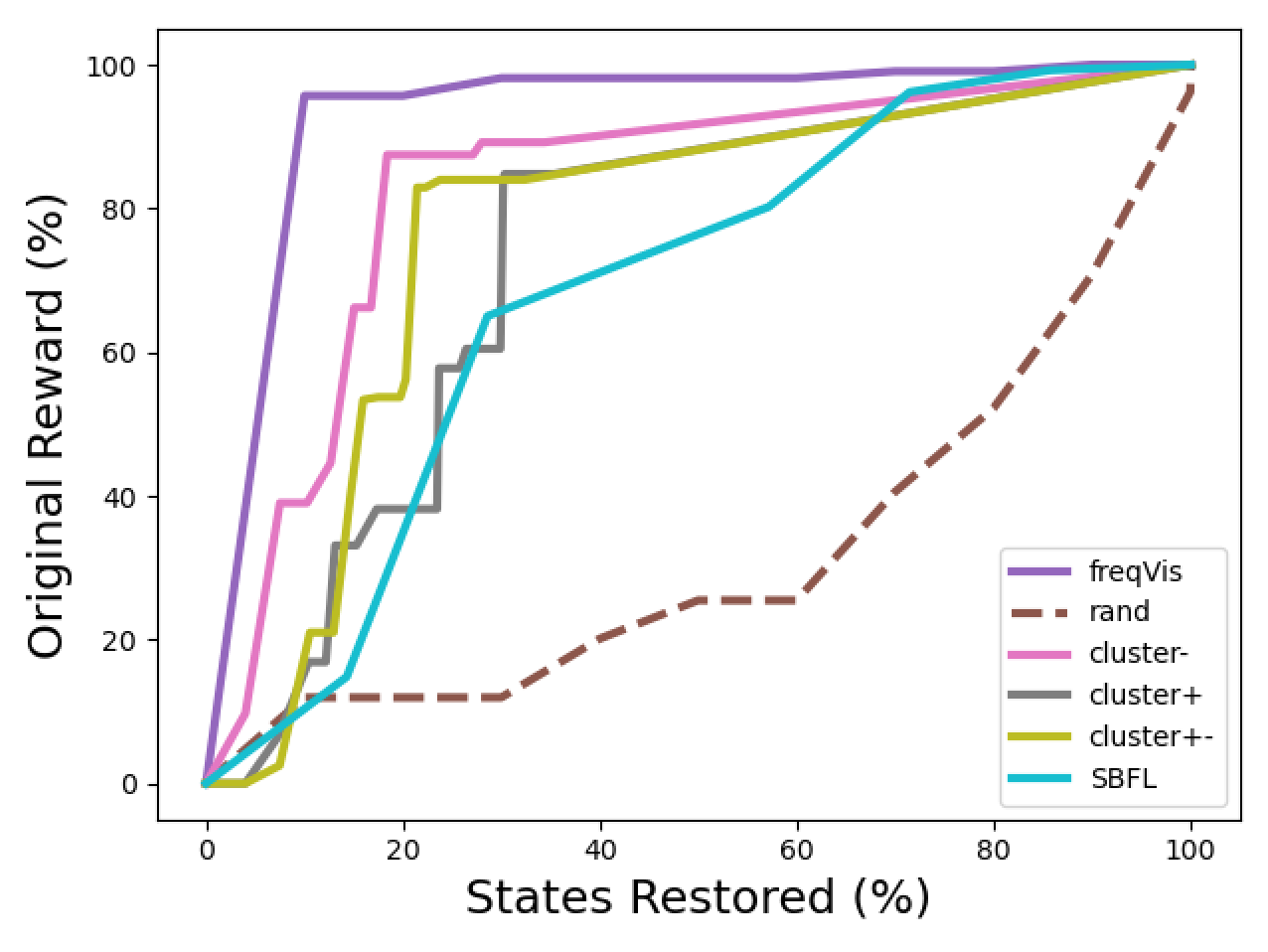
Figure 1: Bowling Reward by States Restored

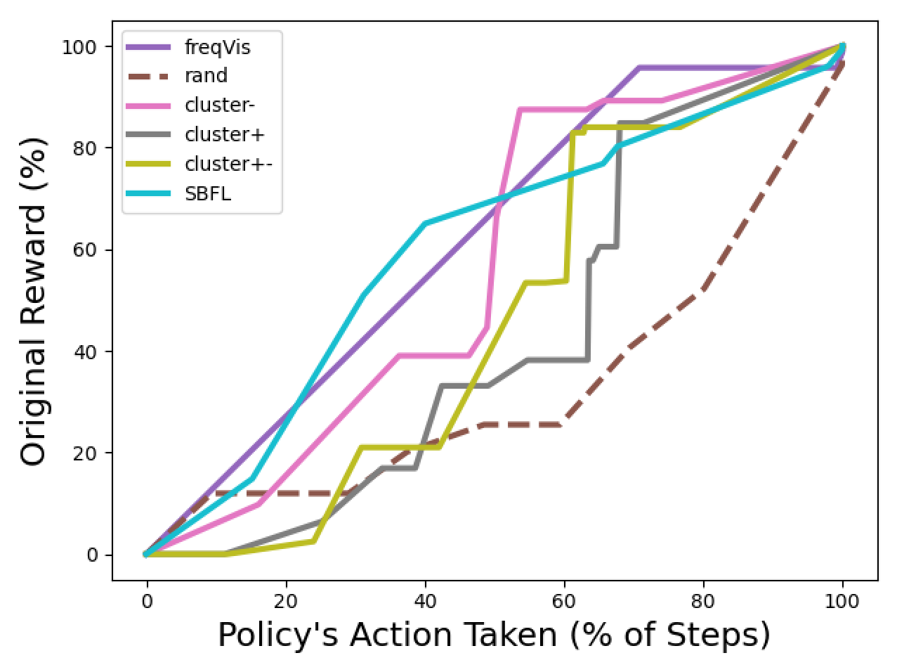
Figure 2: Bowling Reward by Actions Restored

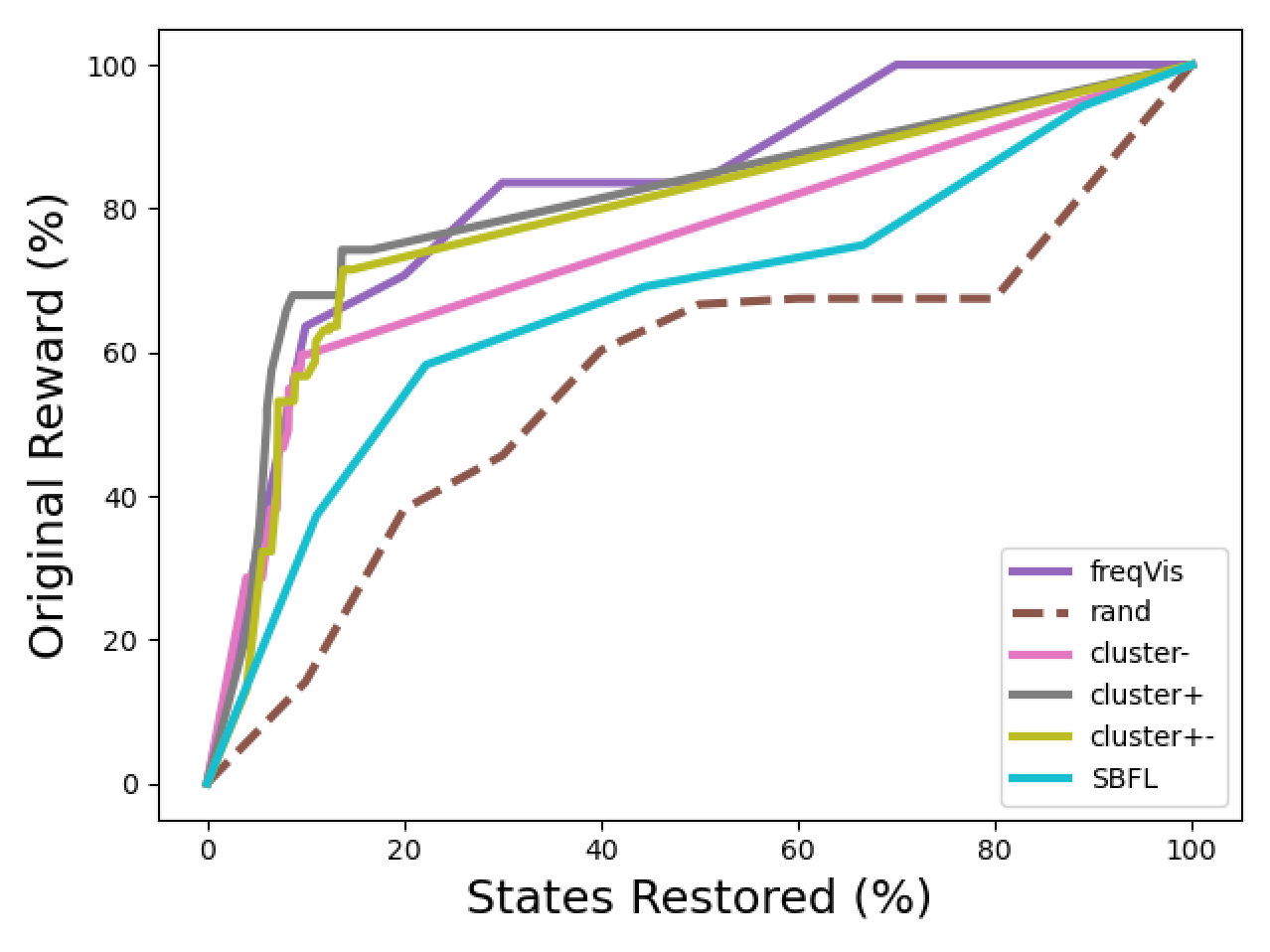
Figure 3: Krull Reward by States Restored

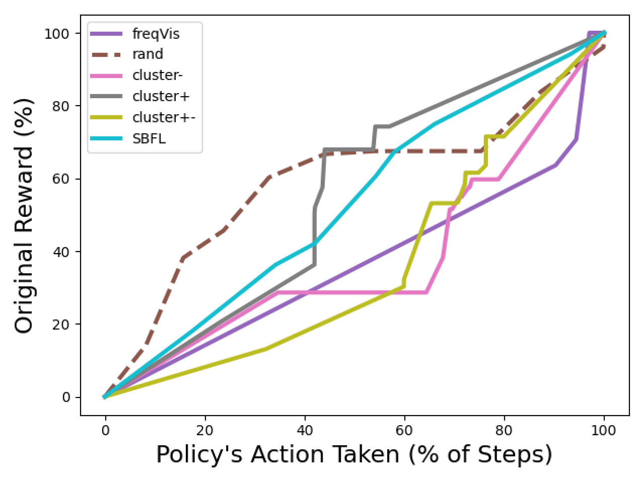
Figure 4: Krull Reward by Actions Restored

We find that in some environments one or more of our clustering methods outperforms SBFL, FreqVis, and Rand. There are many atari environments in which clustering outperforms SBFL but not FreqVis or vice-versa; the Bowling and Krull Atari games seemed best suited to the clustering process’s strengths among the environments we explored.

Fig 1 shows the comparison of methods by our first metric in the Bowling environment. All three clustering processes noticeably outperform SBFL, accomplishing most of the original reward with a significantly smaller portion of the state space restored. They do underperform FreqVis by this metric, however that is typically to be expected, as by definition FreqVis restores most of the actions by restoring only a small part of the state space. Our second metric which is shown in Fig 2 is more suited to comparing a ranking’s effectiveness against FreqVis. Here, the “cluster-” method mostly keeps pace with FreqVis and even reaches 80% reward before it (though FreqVis achieves $95\%$ reward faster).

Fig 3 shows the comparative performance by our first metric in the Krull environment. As in Bowling, all three clustering methods noticeably outperform SBFL, but “cluster+” and “cluster+-” seem on par with FreqVis even in the first metric. The addition of the second metric in Fig 4 reveals that FreqVis is not in fact well suited to the Krull environment, and “cluster+” outperforms all other methods. Based on these results, we extrapolate that Krull has a set of states that are not observed significantly more often than others (as Freqvis extracts) and do not individually have a significant effect on reward (as SBFL extracts), but collectively synergize to restore a significant proportion of the reward without requiring the restoration of larger parts of the state space.

Conclusions and Discussion

FreqVis, SBFL, and our clustering procedure each likely have their own place depending on the size, complexity, and characteristics of the environment. We suggest using a portfolio platform that includes a number of techniques, when trying to find an optimal pruning of a policy. It is likely that our clustering method works significantly better when a feature based encoder is employed rather than simple abstractions such as grey-scaling or discretizing. This may be feasible given recent work in model-based reinforcement learning such as the development of the CLIP algorithm (Radford et al. 2021) which learns an off-policy encoding of the state space without losing significant information and has the potential to expose pseudo-features.

References

- Brockman et al. (2016) Brockman, G.; Cheung, V.; Pettersson, L.; Schneider, J.; Schulman, J.; Tang, J.; and Zaremba, W. 2016. OpenAI Gym. CoRR, abs/1606.01540.
- Chevalier Boisvert, Willems, and Pal (2018) Chevalier Boisvert, M.; Willems, L.; and Pal, S. 2018. Minigrid. https://github.com/Farama-Foundation/Minigrid.
- Gunning and Aha (2019) Gunning, D.; and Aha, D. W. 2019. DARPA’s explainable artificial intelligence program. AI Magazine, 40(2): 44–58.
- Hotelling (1936) Hotelling, H. 1936. Relations Between Two Sets of Variates. Biometrika, 28(3/4): 321–377.
- Jones (1972) Jones, K. S. 1972. A statistical interpretation of term specificity and its application in retrieval. Journal of Documentation, 28(1): 11–21.
- Lewis, Li, and Sycara (2020) Lewis, M.; Li, H.; and Sycara, K. 2020. Deep Learning, Transparency and Trust in Human Robot Teamwork. Preprint.
- McNamee and Chockler (2022) McNamee, D.; and Chockler, H. 2022. Causal Policy Ranking. In ICLR2022 Workshop on the Elements of Reasoning: Objects, Structure and Causality.
- Pouget et al. (2021) Pouget, H.; Chockler, H.; Sun, Y.; and Kroening, D. 2021. Ranking Policy Decisions. In Proceedings of Annual Conference on Neural Information Processing Systems (NeurIPS), 8702–8713.
- Radford et al. (2021) Radford, A.; Kim, J. W.; Hallacy, C.; Ramesh, A.; Goh, G.; Agarwal, S.; Sastry, G.; Askell, A.; Mishkin, P.; Clark, J.; Krueger, G.; and Sutskever, I. 2021. Learning Transferable Visual Models From Natural Language Supervision. arXiv:2103.00020.
- Sutton and Barto (2018) Sutton, R.; and Barto, A. 2018. Reinforcement Learning: An Introduction. MIT Press.
- Sutton, Precup, and Singh (1999) Sutton, R.; Precup, D.; and Singh, S. 1999. Between MDPs and Semi-MDPs: A Framework for Temporal Abstraction in Reinforcement Learning. Artificial Intelligence, 112: 181 – 211.