Convolutional Neural Networks for Neuroimaging in Parkinson’s Disease: Is Preprocessing Needed?

Abstract

Spatial and intensity normalization are nowadays a prerequisite for neuroimaging analysis. Influenced by voxel-wise and other univariate comparisons, where these corrections are key, they are commonly applied to any type of analysis and imaging modalities. Nuclear imaging modalities such as PET-FDG or FP-CIT SPECT, a common modality used in Parkinson’s Disease diagnosis, are especially dependent on intensity normalization. However, these steps are computationally expensive and furthermore, they may introduce deformations in the images, altering the information contained in them. Convolutional Neural Networks (CNNs), for their part, introduce position invariance to pattern recognition, and have been proven to classify objects regardless of their orientation, size, angle, etc. Therefore, a question arises: how well can CNNs account for spatial and intensity differences when analysing nuclear brain imaging? Are spatial and intensity normalization still needed? To answer this question, we have trained four different CNN models based on well-established architectures, using or not different spatial and intensity normalization preprocessing. The results show that a sufficiently complex model such as our three-dimensional version of the ALEXNET can effectively account for spatial differences, achieving a diagnosis accuracy of 94.1% with an area under the ROC curve of 0.984. The visualization of the differences via saliency maps shows that these models are correctly finding patterns that match those found in the literature, without the need of applying any complex spatial normalization procedure. However, the intensity normalization -and its type- is revealed as very influential in the results and accuracy of the trained model, and therefore must be well accounted.

1 Introduction

Deep learning (LeCun, Bengio, and Hinton 2015) is currently a major trend in every research field. Its flexibility, adaptability and its unprecedented accuracy in image classification has motivated its adoption in many disciplines ranging from speech (Kim, Kim, and Seo 2004; Hinton et al. 2012) or pattern recognition (Garrido et al. 2016) to drug discovery (Gawehn, Hiss, and Schneider 2016) and genomics (Alipanahi et al. 2015). It is also gradually opening up in medical image analysis (Liao et al. 2013; Olson and Perry 2013; Xu et al. 2014; Greenspan, Ginneken, and Summers 2016; Ortiz et al. 2016; Martín-López et al. 2017), and particularly in neuroimaging (Martín-López et al. 2017; Ortiz et al. 2016; Olson and Perry 2013), where large amounts of data are analysed through well-established processes.

Large-scale analysis of neuroimaging such as the Statistical Parametric Mapping (SPM) (Friston et al. 2007) or many other multivariate learning techniques (I. A. Illán et al., n.d.; Fermín Segovia et al. 2012; Saxena et al. 1998; Gorriz et al. 2017) require a multi-step preprocessing of brain images. These steps include: motion correction, realignment, linear or non-linear registration to a common space (frequently the MNI space), segmentation, smoothing, intensity normalization, etc (F. J. Martinez-Murcia, Górriz, and Ramírez 2016). Of these, non-linear registration to a standard template -also known as spatial normalization- is present in the vast majority of imaging tools, under the assumption that the same anatomical positions must lay in the same spatial coordinate in order to perform the analysis. This is true for Computer Aided Diagnosis (CAD) systems using more traditional machine learning algorithms such as Principal Component Analysis (PCA) (López et al. 2011), or the Support Vector Machine (SVM) (I. A. Illán et al., n.d.; Fermín Segovia et al. 2012; Saxena et al. 1998; Gorriz et al. 2017; F. Martínez-Murcia et al. 2014) and Random Forests (Ramírez et al. 2010) classifiers. However, non-linear spatial normalization introduces local deformations in the shape and size of different regions that may lead to artifacts introduced by the anatomic standardization process (Ishii et al. 2001; Reig et al. 2007; Martino et al. 2013).

Two major categories of neuroimaging can be defined: structural and functional, depending on the information contained within. In the case of functional imaging, intensity normalization is key. It helps to perform a straightforward comparison between intensity level in each image, despite other individual factors such as drug uptake, acquisition time or scanner sensitivity (D. Salas-Gonzalez et al. 2012; I. A. Illán et al., n.d.; Saxena et al. 1998; F. Martínez-Murcia et al. 2014). It can be compared to feature standardization, a fundamental preprocessing in machine learning, especially with learners such as Support Vector Machines or Artificial Neural Networks (ANNs). However, while feature standardization frequently converts each feature in all subjects to be distributed with zero mean and unit variance, intensity normalization changes the intensity levels of each subject independently, according to different parameters such as global or maximum intensity.

Spatial and intensity normalization have been also applied as a part of the preprocessing pipeline in applications of deep learning to medical imaging (Yuvaraj et al. 2016; Francisco Jesús Martinez-Murcia et al. 2017; Hirschauer, Adeli, and Buford 2015). However, deep learning, and in particular Convolutional Neural Networks (CNN) have shown great ability in classifying objects into images regardless of their orientation, size, angle, etc (Morabito et al. 2017; Koziarski and Cyganek 2017; Ortega-Zamorano et al. 2017; Lin, Nie, and Ma 2017; Zhang et al. 2017; Cha, Choi, and Büyüköztürk 2017; Rafiei and Adeli 2015, 2017, 2018; Rafiei et al. 2017; Acharya et al. 2017). Then, a question arises: is spatial and/or intensity normalization needed in neuroimaging applications of deep learning?

In this work we explore the effect of spatial and intensity normalization of neuroimaging in the classification of Parkinson’s Disease (PD) patients from the well-established Parkinson’s Progression Markers Initiative (PPMI), using FP-CIT SPECT images. In Section 2 we present the methodology followed, including a description of the dataset, the spatial and intensity normalization procedures evaluated, a description of our CNN, the data augmentation procedures used and an introduction to the evaluation metrics. In Section 3, the results of this evaluation are presented, and further discussed at Section 4. Finally, in Section 5, some conclusions are drawn.

2 Methodology

2.1 Dataset

Data used in the preparation of this article were obtained from the Parkinson’s Progression Markers Initiative (PPMI) database (www.ppmi-info.org/data). For up-to-date information on the study, visit www.ppmi-info.org. The images in this database were imaged 4 + 0.5 hours after the injection of between 111 and 185 MBq of DaTSCAN. Raw projection data are acquired into a $128\times 128$ matrix stepping each 3 degrees for a total of 120 projection into two 20% symmetric photopeak windows centered on 159 KeV and 122 KeV with a total scan duration of approximately 30 - 45 minutes (Initiative 2010).

A total of $N=642$ DaTSCAN images from this database were used in the preparation of the article. Specifically, the baseline acquisition from $448$ subjects suffering from PD and $194$ normal controls was used. The images, roughly realigned, were then linearly resampled down to a final size of (57,69,57), the input size of the network. Unless stated, these are considered the ‘original’, non-normalized images. For more details on the demographics of this dataset, please check Table LABEL:tbl-demographics.

Table 1: Demographics of the PPMI dataset

Group	Sex	N	Age [STD]
Control	F	65	58.85 [11.95]
	M	129	62.00 [10.74]
PD	F	160	61.49 [9.96]
	M	288	62.89 [9.71]

2.1.1 Spatial Normalization

Spatial normalization is frequently used in neuroimaging studies. It eliminates differences in shape and size of brain, as well as local inhomogeneities due to individual anatomic particularities. It is particularly key in group analysis, where voxel-wise differences are analysed and quantified (F. J. Martinez-Murcia, Górriz, and Ramírez 2016).

In this procedure, individual images are mapped from their individual subject space (image space) to a common reference space, usually stated using a template. The mapping involves the minimization of a cost function that quantifies the differences between the individual image space and the template. The most frequent template is the Montreal Neurological Institute (MNI), set by the International Consortium for Brain Mapping (ICBM) as its standard template, currently in its version ICBM152 (Mazziotta et al. 2001), an average of 152 normal MRI scans in a common space using a nine-parameter linear transformation.

There exist a wide range of global and local transformations that could be categorized in linear transformations (of which the affine transform is the most complex) and elastic transformations and diffeomorphisms. The affine transform converts the old coordinates $(x,y,z)$ to the new common coordinate system $(x^{\prime},y^{\prime},z^{\prime})$ using 12 parameters for translation, rotation, scale, squeeze, shear and others:

$$\hypertarget{eq-affine}{}{\left[\begin{matrix}x^{\prime}\\ y^{\prime}\\ z^{\prime}\\ 1\end{matrix}\right]=\left[\begin{matrix}a_{00}&a_{01}&a_{02}&a_{03}\\ a_{10}&a_{11}&a_{12}&a_{13}\\ a_{20}&a_{21}&a_{22}&a_{23}\\ 0&0&0&1\\ \end{matrix}\right]\left[\begin{matrix}x\\ y\\ z\\ 1\end{matrix}\right]}$$ (1)

A particular case of affine transformation is the similarity transformation, where only scale, translation and rotation are applied. This is often used for motion correction and reorientation of brain images with respect to a reference, and is frequently performed automatically on many imaging equipment.

Affine transforms are applied globally to the whole image. In contrast, modern solutions often refine the output by applying local deformations, in what is known as diffeomorphic transformations, which feature the estimation and application of a warp field. Some examples are SPM (Friston et al. 2007) or Freesurfer (Reuter, Rosas, and Fischl 2010).

The DaTSCAN images from the PPMI dataset are roughly realigned. We will refer to this as non-normalized (given that it is only a similarity transformation that preserves shape). We further preprocessed the images using the SPM12 New Normalize procedure with default parameters, which applied affine and local deformations to achieve the best warping of the images and a custom DaTSCAN template defined in Ref. .

2.2 Intensity Normalization

Intensity normalization is a technique that changes globaly or locally the intensity values of an image in order to ensure that the same intensity levels correspond to similar physical measures. In nuclear imaging, the use of intensity normalization is key in order to compare brain activity or function between subjects. A similar intensity should indicate a similar drug uptake and therefore, differences in these values may be due to different pathologies (F. J. Martínez-Murcia et al. 2012; Fermín Segovia et al. 2012).

Intensity normalization in neuroimaging usually follows the expression:

$$\hat{\mathbf{I}}_{i}=\mathbf{I}_{i}/I_{n,i}$$

where $\mathbf{I}_{i}$ is the image of the $i^{th}$ subject in the dataset, $\hat{\mathbf{I}}_{i}$ is the normalized image, and $I_{n}$ is an intensity normalization value that is computed independently for each subject.

Two normalization strategies will be used in this paper:

• In the Normalization to the maximum, $I_{n}$ is computed as the average of the top 3% intensities in an image. By averaging this top 3% we ensure that the maximum intensity is not an outlier. The resulting image’s intensities will be in the range $(0,1)$.

• For its part, the Integral Normalization (I. A. a. Illán et al. 2012) sets $I_{n}$ to the average of all values in a certain volume the image, in an approximation of the integral. In Parkinson, this is often set to the average of the brain without the specific areas: the striatum; although the influence of these areas is often small, and it can be approximated by the mean of the whole image. This is the procedure followed in this paper.

2.3 Convolutional Neural Networks

Convolutional Neural Networks (CNNs) are becoming increasignly important in the Machine Learning community (Krizhevsky, Sutskever, and Hinton 2012; Ciresan et al. 2011; Ortiz et al. 2016; Fermín Segovia et al. 2016; Sabour, Frosst, and Hinton 2017), especially within the artificial vision and image analysis fields. Since 2012, when an ensemble of CNNs (Krizhevsky, Sutskever, and Hinton 2012) achieved lowest error on the ImageNet classification benchmark (Schmidhuber 2015), CNNs prevail over any other pattern recognition algorithm in the literature in image classification.

CNNs are bioinspired by the convolutional response of neurons, and combine feature extraction and classification in one single architecture. The combination of different convolution and pooling steps is able to recognize different patterns, from low-level features to higher abstractions, depending on the net depth. The set of fully connected layers, similar to a perceptron, placed after convolutional layers, performs the real machine learning. Many architectures combining these and other types of layers can be found throughout the literature (Krizhevsky, Sutskever, and Hinton 2012; Ciresan et al. 2011; Abadi et al. 2015; Payan and Montana 2015; Ortiz et al. 2016; Fermín Segovia et al. 2016; Sabour, Frosst, and Hinton 2017).

One key property that defines CNNs is parameter sharing. All neurons in any convolutional layer share the same weights, saving memory and easing computation of the convolutions. Other properties shared by CNNs are local connectivity of the hidden units and the use of pooling to introduce position invariance, although this latter feature is currently being challenged by newer approaches (Springenberg et al. 2014; Sabour, Frosst, and Hinton 2017)

2.3.1 Convolutional Layer

The convolutional layer is the main component of CNNs. Mathematically, the operation at the convolutional layer takes a tensor $\mathbf{V}_{i-1}$ containing the activation map of the previous layer $(i-1)$-th (for $i=1$ it is the input volume). The $i^{th}$ layer learns a set of $K$ filters $\mathbf{W}_{i}$ with a bias term $\mathbf{b}_{i}$, a vector of length $K$. The mathematical operation performed at the convolutional layer is:

$$\mathbf{V}_{i}=f_{a}\left(\mathbf{W}_{i}*\mathbf{V}_{i-1}+\mathbf{b}_{i}\right)$$

where $f_{a}(*)$ is the activation function (see Sec. Section 2.3.2).

For a three-dimensional environment, $\mathbf{V}_{i-1}$ is of size $H\times W\times D\times C$ (height, width, depth and number of channels), and $\mathbf{W}_{i}$ is of size $P\times Q\times R\times S\times K$, with $K$ the number of filters. The $k^{th}$ convolution term for the $k^{th}$ filter is:

$$\hypertarget{eq-3dconv}{}{\begin{gathered}\mathbf{W}_{ik}*\mathbf{V}_{i-1}=\\ \sum_{u=0}^{P-1}\sum_{v=0}^{Q-1}\sum_{w=0}^{R-1}\big{[}\mathbf{W}_{ik}(P-u,Q-v,R-w)\cdot\\ \mathbf{V}_{i-1}(x+u,y+v,z+w)\big{]}\end{gathered}}$$ (2)

After convolution, the activations of the $K$ filters in layer $i$ are stacked and passed to layer $(i+1)$.

There are a number of hyperparameters that must be set a priori, among them the filter size (usually a cube of $P=Q=R$), which in the literature take frequently values (LeCun et al. 1998; Krizhevsky, Sutskever, and Hinton 2012) of 3, 5 or 7. Other parameters are the number of filters $K$, stride and zero-padding. The number of filters varies a lot in the literature, frequently taking numbers that are a power of 2. The higher this number is, the more patterns (simple in lower layers, more complex in higher layers) our CNN is able to learn. This number is usually high in two-dimensional CNNs (being 48, 96 or 128 frequent values for the first layer) (LeCun et al. 1998; Krizhevsky, Sutskever, and Hinton 2012), and increasing in higher-order layers after dropout. In three-dimensional layers, however, this number is smaller, due to hardware requirements.

Stride, for its part, controls the step at which the convolution is computer, namely how much overlapping there is between convolutions. That defines the so called ‘receptive field’ of a neuron, which is the part of the image to which a neuron is connected. A stride of 1 means that the convolution is performed at each voxel of the input. Higher strides mean less overlapping between receptive fields and smaller volumes in the output.

Finally, zero-padding provides control of the output volume by padding the input volume with zeros. That way, we can let the output volume be the same size as the input volume, which is desirable in some cases.

2.3.2 Activations

The activation is a function used to compute the output of a layer, common to all types of ANNs. It is applied after a single value $z$ -weighted sum of inputs or the sum of all convolutions- is computed in that layer, and is often consider to ‘fire’ the neuron signal. Many activation functions exist, among them the first function to be used in ANNs: the hyperbolic tangent or $\tanh$. In this work we use three different activation functions.

First, in the convolutional layers we have chosen the Rectified Linear Unit (ReLU), a non-saturating activation function.

$$f_{RELU}(z)=\max(0,z)$$

It has gained a lot of popularity thanks to its properties, especially for making the training procedure much faster than other approaches, since its derivative has a smaller computational cost. It has been proven that this reduction in time comes without loss of generalization ability (Krizhevsky, Sutskever, and Hinton 2012), which makes it optimum for our purpose.

Second, we also wanted to assess the novel Self-Normalized Neural Networks (SNNs) (Klambauer et al. 2017) in this context. SNNs are designed in order to avoid vanishing and exploding gradients during the training iterations, introducing the Scaled Exponential Linear Unit (SELU):

$$f_{SELU}(z)=\lambda\begin{cases}z&\text{if }z\geq 0\\ \alpha e^{z}-\alpha&\text{if }z<0\\ \end{cases}$$

This SELU function, used with the default parameters calculated in Ref  for the typical normalization $(\mu,\nu)=(0,1)$ used in batch normalization, which correspond to $\alpha\approx 1.6733$ and $\lambda\approx 1.0507$. This function introduces self-normalizing properties at the output of each layer which in the case of Feed Forward Networks has proven to propagate zero-mean and unit-variance gaussian-distributed outputs through the network even in noisy environments.

The last activation function to be used is the well-established softmax, used at the output layer. The softmax activation function for the $j^{th}$ neuron (devoted to the $j^{th}$ class in the problem) in the output layer follows the expression:

$$\sigma(\mathbf{z})_{j}=\frac{e^{z_{j}}}{\sum_{k=1}^{K}e^{z_{k}}}\quad\text{for}j=1,\dots K$$

where $z_{j}=\mathbf{x}^{T}\mathbf{w}_{j}$, being $\mathbf{x}$ the outputs of the previous layer, and $\mathbf{w}_{j}$ the weights of the connections of the $j^{th}$ neuron.

2.3.3 Max Pooling

A key operation in CNNs is pooling, which provides a sort of positional invariance of the patterns that fire up neuron activations by reducing the input space of subsequent layers while keeping the receptive field of the filters. The most common type of pooling is Max Pooling (MaxPool), which keeps the maximum value over a $M\times M\times M$ block of the activation layer in the case of 3D layers. Furthermore, MaxPool also prevents the following layers from processing non-maximum values, therefore reducing computational load.

Some works are starting to eliminate MaxPooling layers from CNN setups (Springenberg et al. 2014), especially in recent capsule networks, where they are being replaced by dynamic routing (Sabour, Frosst, and Hinton 2017). This provides the network with positional equivariance, which, in contrast to the Pooling invariance, preserves the relative positions of the different patterns detected at lower level layers. However, we have opted to replicate well known models such as LENET and ALEXNET in three-dimensional environments, and therefore, we keep the MaxPool layers present in these models, with different block sizes.

2.3.4 Dense Layers

Fully connected layers, also known as dense layers, are the components of typical ANN examples such as the multilayer perceptron (MLP). In dense layers all neurons are connected to all outputs from the previous layer. In CNNs, several dense layers are usually placed after a set of convolution and pooling layers. They can be considered the high-level reasoning part of the CNN. In these cases, the output of the $j^{th}$ neuron will be computed by:

$$z_{j}=f(\mathbf{x}^{T}\mathbf{w}_{j})$$

where $f()$ is any activation function. In CNNs is frequent to have several dense layers with RELU activation and finally, the last layer uses the softmax activation function.

2.3.5 Dropout

Dropout is a method intended to reduce overfitting in fully connected layers (Schmidhuber 2015). With this method, only a percentage $1-p$ of the neurons of one layer are active in one training iteration. In the next iteration, the inactive neurons will recover their past weight matrix, and the procedure is repeated. At testing time, all neurons are active, and therefore the output of the neurons is weighted by a factor of $p$, approximating the use of all possible $2^{n}$ networks.

A particular case of dropout is AlphaDropout (Klambauer et al. 2017), devised originally for SNNs. It keeps the mean and variance of inputs to their original values, therefore ensuring the self-normalizing assumption even after dropout. Instead of turning off the neurons, establishes their weight as the negative saturation value of the function.

2.3.6 Loss functions

The CNN is trained with the objective of optimizing a loss function. This is often chosen as a result of trial and error, and is hardly reported in many CNN papers. In this work, we have tried two different functions with different properties, in order to see their influence in the convergence of the models.

The first strategy here is to maximize the cross-entropy (x-e), a measure of similarity between the real output $y_{i}$ and the predicted output $\hat{y}_{i}$ of the classifier for all $N$ images in a training batch. This is defined by:

$$\ell_{x-e}=\ -\frac{1}{N}\sum_{i=1}^{N}\ \bigg{[}y_{i}\log\hat{y}_{i}\bigg{]}$$

A second approach, more frequent in regression but gaining ground in classification, is logcosh (lc), or the $\log(cosh(x))$. It is similar to other functions, but twice differentiable everywhere, and approximately equal to $(x^{2})/2$ for small x and to $\text{abs}(x)-\log(2)$ for large x. It has the advantage of working similarly to the mean squared error, but being not so strongly affected by occasional wrong predictions:

$$\ell_{lc}=-\frac{1}{N}\sum_{i=1}^{N}\bigg{[}\log(\cosh(\hat{y}_{i}-y_{i}))\bigg{]}$$

2.4 Our models

We have tested two different CNN models, based on a three-dimensional implementation of well-established architectures. We assume the three-dimensional convolutions stated in Equation 2, and a three-dimensional max pooling. The number of filters and number of neurons in dense layers is smaller than in their 2D counterparts, mainly due to the memory restrictions and the fact that this is a binary classification problem:

• LENET53D is a 3D implementation of the LeNet-5 (LeCun et al. 1998) as in the original paper architecture. This architecture is composed of 5 layers, combining 2 convolutional, 2 max-pooling and 1 fully connected layer as in the structure found in Figure 1.

• ALEXNET3D is a 3D implementation of the AlexNet (Krizhevsky, Sutskever, and Hinton 2012), which uses five convolutional layers, two fully connected layers and three max-pooling layers, following the architecture found at Figure 1.

These two models have been also implemented with the SELU activation function. These two models, LENET53D-SELU and ALEXNET3D-SELU, have the same number of parameters that their SELU counterparts, and only differ in the activation function, the initialization of the weights at each layer, and the dropout technique suggested in Ref .

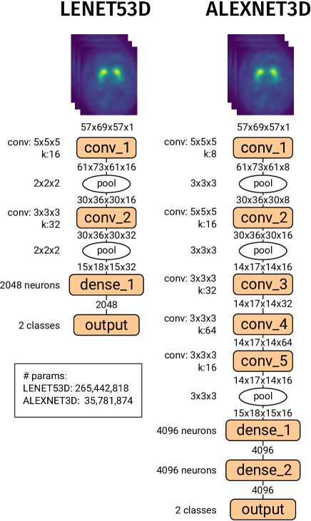
Figure 1: Outline of the LENET53D and ALEXNET3D models used in this article, including the size of convolutions and pooling, number of filters, size of tensors and total number of parameters.

2.4.1 Evaluation

Multiple evaluation parameters have been used in the results section, considering a binary classification problem (PD vs. controls): accuracy, sensitivity, specificity, balanced accuracy and F1-score -all derived from the confusion matrix-, the Receiver Operating Characteristic (ROC) curve, and the Area Under the ROC Curve (AUC). The confusion matrix contains the number of True Positives (TP), True Negatives (TN), False Positives (FP) and False Negatives (FN) of the prediction of the trained model, from which we can compute the parameters:

acc $$=\frac{TP+TN}{TP+TN+FP+FN}$$

sens $$=\frac{TP}{TP+FN}$$

spec $$=\frac{TN}{TN+FP}$$

F1-score $$=\frac{2TP}{2TP+FN+FP}$$

bal. acc $$=\frac{\text{sens}+\text{spec}}{2}$$

These parameters have been computed within a cross-validation scheme, namely a 10-fold stratified cross-validation, where the distribution of classes within each fold is similar to the distribution of classes in the whole dataset (Kohavi and John 1995). We have trained the different models over 60 epochs with a batch size of 64, and using class weights equal to the proportion of samples in each class (due to our imbalanced dataset).

The ROC curve depicts the sensitivity over one minus the specificity at different thresholds of a classifier. This curve can be computed by ranking the softmax values at the output layer for each class, and depicting each point depending on whether it is a TP or FP (Hanley and McNeil 1982). It yields a visual comparison of different methods, frequently used in many works (F. J. Martínez-Murcia et al. 2012; F. Segovia et al. 2012; I. A. a. Illán et al. 2012). We can integrate each curve to obtain the AUC, another estimate of the overall performance, which is reported for each curve. Note that we will use a name convention of [no$|$int$|$max]_[u$|$w] to abbreviate legends in the figures of the result section, where ‘no’, ‘int’, and ‘max’ represent the types of intensity normalization and ‘w’ and ‘u’ state if we apply or not spatial normalization respectively.

For assessing the most relevant regions, we use saliency maps (Simonyan, Vedaldi, and Zisserman 2013) which, in brief, highlight the salient image regions that contribute the most to the assigned class. This is done by computing the gradient of the output category with respect to a sample input image as in:

$$\frac{\partial\text{output}}{\partial I_{\text{input}}}$$

This quantifies the changes in the output score with respect to a small change in the input. This eventually leads to a map the same size of the original images where the most relevant voxels are highlighted. To generate the maps we have used the keras-vis (Kotikalapudi and contributors 2017) python toolbox.

3 Results

Each proposed model has been trained and tested via cross-validation on a 642-subject dataset containing DaTSCAN images from PD and normal control. For more details on the demographics, please check Table LABEL:tbl-demographics. The particular results for each model are detailed below.

3.1 Results for the LENET53D model

We use a LENET model analogous to the first five-layer LENET5 proposed in Ref. , although using 3D convolutions instead of 2D. The performance of this model, depending on the preprocessing, and loss function applied can be checked at Table LABEL:tbl-lenet_perf_all.

Table 2: Performance values and standard deviation of the different preprocessing pipelines in the LENET53D model.

S -norm	I- norm.	loss	acc [ std]	sens. [ std]	spec. [ std]	f1	bal. acc
yes	no	x-e	0.500 [0. 198]	0.500 [0. 500]	0.500 [0. 500]	0.500	0.500
yes	no	lc	0.461 [0. 194]	0.400 [0. 490]	0.600 [0. 500]	0.444	0.500
yes	max	x-e	0.760 [0. 072]	0.922 [0. 090]	0.389 [0. 318]	0.728	0.656
yes	max	lc	0.791 [0. 087]	0.929 [0.08 1]	0.474 [0. 257]	0.757	0.702
yes	int	x-e	0.872 [0. 109]	0.891 [0. 139]	0.827 [0. 228]	0.864	0.859
yes	int	lc	0.922 [0.03 7]	0.918 [0. 054]	0.932 [0.08 6]	0. 924	0. 925
no	no	x-e	0.464 [0. 199]	0.369 [0. 460]	0.685 [0. 482]	0.438	0.527
no	no	lc	0.494 [0. 193]	0.487 [0. 488]	0.510 [0. 490]	0.492	0.498
no	max	x-e	0.494 [0. 192]	0.449 [0. 458]	0.597 [0. 456]	0.485	0.523
no	max	lc	0.866 [0. 205]	0.860 [0. 288]	0.879 [0. 292]	0.868	0.869
no	int	x-e	0.575 [0. 191]	0.561 [0. 351]	0.604 [0. 345]	0.574	0.583
no	int	lc	0.949 [0.02 5]	0.940 [0.04 6]	0.969 [0.05 1]	0. 954	0. 954

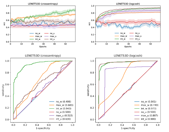
Figure 2: Performance of the different normalization methods and loss functions in the LENET53D architecture. Upper part: evolution (mean and standard deviation) of the training accuracy in different epochs; lower part: ROC curves at the operation point.

The behaviour of the LENET53D model is quite complex. When there is spatial normalization, the influence of the loss function is minimal, although the logcosh (lc) often performs better than the cross-entropy (x-e). The behaviour is, however, very different when there is no spatial normalization applied. In this case, the logcosh achieves significantly better performance than the models trained with cross-entropy, in any intensity normalization case. This behaviour is even more clear in @#fig-lenet5-perf, where the convergence of the system using this function is clearly faster than when using cross-entropy, for any combination of spatial and intensity normalization. This even helps the model to perform similarly regardless of the intensity normalization.

Regarding the data, intensity normalization may be key for the model to correctly account for PKS-related patterns. Of all intensity normalization strategies, the integral normalization always perform better than the normalization to the maximum, even when there is no spatial normalization applied.

3.2 Results for the LENET53D-SELU model

The LENET53D-SELU is identical to the LENET53D, but using SELU as activation function, a different random initialization and the custom dropout defined at Section 2.3.2 and Section 2.3.5.

Table 3: Performance values and standard deviation of the different preprocessing pipelines in the LENET53D-SELU model.

S -norm	I- norm.	loss	acc [ std]	sens. [ std]	spec. [ std]	f1	bal. acc
yes	no	x-e	0.302 [0. 005]	0.000 [0. 000]	1.000 [0. 500]	nan	0.500
yes	no	lc	0.302 [0. 005]	0.000 [0. 000]	1.000 [0. 500]	nan	0.500
yes	max	x-e	0.511 [0. 146]	0.516 [0. 318]	0.499 [0. 303]	0.511	0.507
yes	max	lc	0.617 [0.06 7]	0.665 [0.08 8]	0.506 [0. 143]	0. 616	0.585
yes	int	x-e	0.460 [0. 194]	0.400 [0. 490]	0.600 [0. 500]	0.444	0.500
yes	int	lc	0.556 [0. 184]	0.447 [0. 345]	0.808 [0.37 6]	0.545	0. 627
no	no	x-e	0.540 [0. 194]	0.600 [0. 490]	0.400 [0. 500]	0.545	0.500
no	no	lc	0.542 [0. 193]	0.600 [0. 490]	0.400 [0. 500]	0.545	0.500
no	max	x-e	0.618 [0.15 8]	0.800 [0.40 0]	0.200 [0. 500]	0. 615	0.500
no	max	lc	0.581 [0. 195]	0.593 [0. 438]	0.553 [0. 451]	0.581	0.573
no	int	x-e	0.421 [0. 181]	0.300 [0. 458]	0.700 [0. 500]	0.375	0.500
no	int	lc	0.609 [0. 252]	0.587 [0. 472]	0.663 [0.42 8]	0.610	0. 625

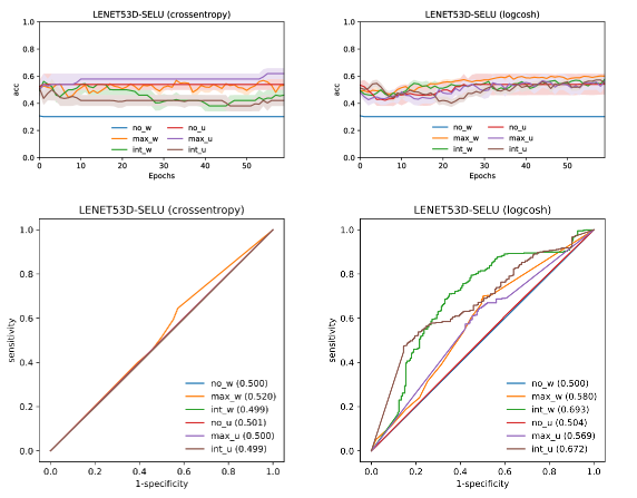
Figure 3: Performance of the different normalization methods and loss functions in the LENET53D-SELU architecture. Upper part: evolution (mean and standard deviation) of the training accuracy in different epochs; lower part: ROC curves at the operation point.

The results are much poorer than in its regular ReLU counterpart. There is no sign of convergence when using the cross-entropy loss function, as seen in Figure 3, nor any difference with a random classifier (see ROC curve). By looking at the sensitivities and specificities of Table LABEL:tbl-lenet_selu_perf_all, it is evident that the classifier is biased, yielding sensitivities multiples of 0.1, which is probably taking all samples as any of the classes at random in each cross-validation iteration.

The logcosh function, although still biased, makes for a better predictor, particularly in the case of integral normalization and spatially normalized images. However, the convergence, if any, is very slow, and after 60 training epochs there is no evidence that the loss is going to decrease. Still, compared to the crossentropy loss function, the logcosh makes the system slightly evolve, which may be an indication of possible learning.

3.3 Results for the ALEXNET3D model

Table LABEL:tbl-alex_perf_all_ce shows the cross-validated performance values obtained for the database under each preprocessing scheme. Under this model, intensity normalization seems key to a good performance. The best performance is obtained with the images using integral intensity normalization, regardless of the spatial normalization. In the case of un-normalized images, the accuracy is almost 94%, with the highest specificity rate -which is key in this unbalanced dataset-. However, when using registered images, the performance does not drop significantly, and in the case of the images normalized to the maximum, the performance even increases.

Table 4: Performance values and standard deviation of the different preprocessing pipelines in the ALEXNET3D model.

S -norm	I- norm.	loss	acc [ std]	sens. [ std]	spec. [ std]	f1	bal. acc
yes	no	x-e	0.498 [0. 198]	0.500 [0. 500]	0.500 [0. 500]	0.500	0.500
yes	no	lc	0.500 [0. 198]	0.500 [0. 500]	0.500 [0. 500]	0.500	0.500
yes	max	x-e	0.793 [0. 064]	0.922 [0. 053]	0.496 [0. 239]	0.760	0.709
yes	max	lc	0.788 [0. 042]	0.967 [0.02 9]	0.378 [0. 320]	0.747	0.672
yes	int	x-e	0.897 [0. 177]	0.869 [0. 234]	0.964 [0. 175]	0.912	0.916
yes	int	lc	0.907 [0.16 4]	0.880 [0. 208]	0.968 [0.16 0]	0. 921	0. 924
no	no	x-e	0.556 [0. 174]	0.649 [0. 423]	0.341 [0. 447]	0.562	0.495
no	no	lc	0.572 [0. 155]	0.662 [0. 359]	0.362 [0. 384]	0.575	0.512
no	max	x-e	0.617 [0. 215]	0.572 [0. 308]	0.719 [0. 306]	0.617	0.645
no	max	lc	0.601 [0. 235]	0.598 [0. 428]	0.608 [0. 425]	0.601	0.603
no	int	x-e	0.941 [0.04 5]	0.933 [0.05 8]	0.958 [0. 079]	0. 945	0. 946
no	int	lc	0.931 [0. 053]	0.915 [0. 079]	0.969 [0.07 2]	0.941	0.942

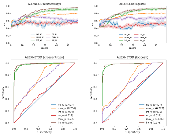
Figure 4: Performance of the different normalization methods and loss functions in the ALEXNET3D architecture. Upper part: evolution (mean and standard deviation) of the training accuracy in different epochs; lower part: ROC curves at the operation point.

The loss function has little impact in this case, as it can be seen from Table LABEL:tbl-alex_perf_all_ce and Figure 4. The convergence is similar both with cross-entropy and logcosh, and the AUC is similarly high in any case that uses integral intensity normalization, followed by normalization to the maximum, and values approximately of a random classifier when not using intensity normalization.

3.4 Results for the ALEXNET3D-SELU model

The SELU counterpart of the ALEXNET3D drops the performance again, as it can be seen in Table LABEL:tbl-alex_selu_perf_all_ce. Its poorer results, regardless of spatial or intensity normalization, can again be attributed to the classifier randomly assigning the same class to all samples in each cross-validation iteration.

Table 5: Performance values and standard deviation of the different preprocessing pipelines in the ALEXNET3D-SELU model.

S -norm	I- norm.	loss	acc [ std]	sens. [ std]	spec. [ std]	f1	bal. acc
yes	no	x-e	0.302 [0. 005]	0.000 [0. 000]	1.000 [0. 500]	nan	0.500
yes	no	lc	0.302 [0. 005]	0.000 [0. 000]	1.000 [0. 500]	nan	0.500
yes	max	x-e	0.414 [0. 172]	0.276 [0. 426]	0.735 [0. 479]	0.358	0.505
yes	max	lc	0.618 [0. 068]	0.667 [0. 091]	0.506 [0. 144]	0.617	0.587
yes	int	x-e	0.659 [0. 119]	0.900 [0.30 0]	0.100 [0. 500]	0.643	0.500
yes	int	lc	0.670 [0.29 7]	0.564 [0. 453]	0.916 [0.37 7]	0. 685	0. 740
no	no	x-e	0.581 [0.18 1]	0.700 [0.45 8]	0.300 [0. 500]	0. 583	0.500
no	no	lc	0.537 [0. 194]	0.600 [0. 490]	0.400 [0. 500]	0.545	0.500
no	max	x-e	0.540 [0. 194]	0.600 [0. 490]	0.400 [0. 500]	0.545	0.500
no	max	lc	0.537 [0. 194]	0.600 [0. 490]	0.400 [0. 500]	0.545	0.500
no	int	x-e	0.498 [0. 198]	0.500 [0. 500]	0.500 [0. 500]	0.500	0.500
no	int	lc	0.505 [0. 257]	0.351 [0. 444]	0.862 [0.44 8]	0.472	0. 607

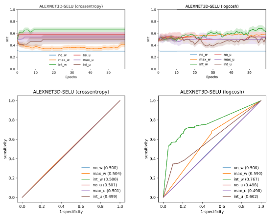
Figure 5: Performance of the different normalization methods and loss functions in the ALEXNET3D-SELU architecture. Upper part: evolution (mean and standard deviation) of the training accuracy in different epochs; lower part: ROC curves at the operation point.

The main difference can be seen when comparing loss functions, as depicted in Figure 5. While the cross-entropy makes the system hardly evolve with the training iterations, the logcosh seems to be increasing the performance, although very slowly. After 60 iterations, the system achieves an AUC of 0.76 when using spatially and intensity normalized images, which is still an improvement over the other preprocessing strategies.

4 Discussion

CNNs are gaining ground in the computer vision community, thanks in part to their ability to recognize patterns with positional invariance. This key feature could be exported to neuroimaging analysis, where spatial normalization has been the norm in the latest 20 years, mainly due to the prevalence of voxel-wise analyses (F. J. Martinez-Murcia, Górriz, and Ramírez 2016).

MaxPooling is partially responsible for this positional invariance. It allows the combination of different simple patterns, computed in the first layers, to account for complex patterns found in latter layers. An increasing number of voices are raising against MaxPool (Springenberg et al. 2014; Sabour, Frosst, and Hinton 2017), pointing to this positional invariance is not equivariance, and that a similar combination of low-level features without a knowledge of their relative position could lead to misclassification (Sabour, Frosst, and Hinton 2017). In this context, capsule networks (Sabour, Frosst, and Hinton 2017) established dynamic routing to account for these differences. However, these are still useful, especially in environments such as neuroimaging, where the images are very similar. In these images the systems find subtle differences in function and/or anatomy, and large-scale artifacts such as switching lobes are very unlikely to occur. Furthermore, MaxPool could be of great help in images where smoothness is an inherent quality (Boureau, Ponce, and LeCun 2010), by selecting larger features without loss of generality.

We have tested two different models, with two variations in each, involving the ReLU and SELU activation functions. Overall, the models using SELU feature a poorer performance, similar to a classifier randomly assigning a certain class to all inputs. Subtle increments in performance can be appreciated with the logcosh loss function, in contrast to cross-entropy. This differs from the original paper using SELU (Klambauer et al. 2017), which used cross-entropy as learning function. While the SELU function was proposed to overcome problems such as vanishing and exploding gradients associated to ReLU in deep dense networks, we could not prove any improvement in our deep CNN. Only the ALEXNET3D-SELU model started to show some performance increment after 60 epochs of training, which by any means indicates a much slower convergence than their ReLU counterparts.

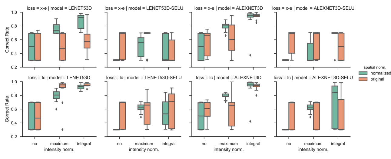
Figure 6: Boxplot of the accuracy rate over the 10 fold cross-validation for each model (columns), loss function (rows), intensity (x axis) and spatial normalization (color).

The main objective of this work was to test whether the typical preprocessing in neuroimaging was needed in a CNN-DL environment. To do so, we used images with and without applying spatial and/or intensity normalization. By looking at the results, summarized at Figure 6, the overall conclusion is that intensity normalization is key for CNNs to learn patterns related to PKS in our dataset, and it has a significant effect, being the most effective the integral normalization. There are many examples of the benefits of intensity normalization in FP-CIT and other nuclear imaging modalities when using traditional machine learning, e.g. Support Vector Machines or Principal Component Analysis (I. A. Illán et al., n.d.; F. Segovia et al. 2012; Diego Salas-Gonzalez et al. 2009; Górriz et al. 2011). However, while the performance gain was obvious in these cases, the difference between normalization strategies was subtle. In our CNN, integral normalization leads to larger performance (see ALEXNET3D and LENET53D with the logcosh function), whereas the impact of the normalization to the maximum is significantly smaller. This paves the way to a more thorough analysis of intensity normalization strategies in deep learning for neuroimaging using newer strategies, for instance, those based on heavy-tailed distributions (Diego Salas-Gonzalez et al. 2013) or Standard Uptake Values (SUV) when the injected dose and patient weight is available.

As for the spatial normalization, is utility could be argued. In shallower networks such as LENET53D, it plays a more significant role, especially when the loss function is cross-entropy. However, when using the ALEXNET3D model, the influence of the spatial normalization is not significant at all, neither altering the final performance nor the speed of convergence. This could mainly be due to the CNNs accounting for differences in alignment, rotation, scale or others. Therefore, we might hypothesize that the deeper the network is, the less the spatial normalization is needed.

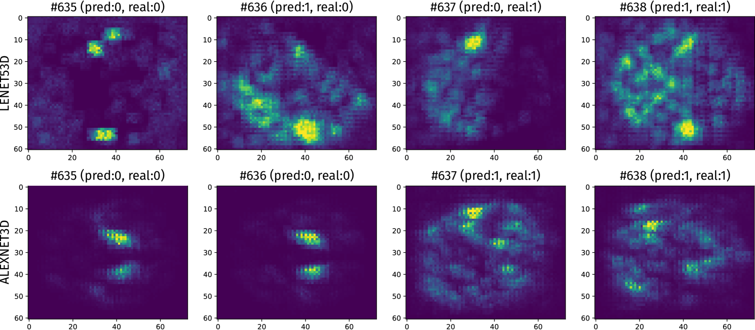
Figure 7: Saliency maps for the LENET53D (first row) and ALEXNET3D (second row) models, in four sample images (numbers 635, 636, 637 and 638) with integral normalization and no spatial normalization applied (u_int). Only the maps for the predicted class, at neurons 0 for class control and neuron 1 for PKS, are shown.

However, recent research (Iacca et al. 2012; Pan et al. 2017) suggests that simple metaheuristics may work better than complex metaheuristics. In addition, the computational complexity of a deeper model is comparable to the cost of spatial standardization in the latest software, for example, SPM or Freesurfer. Therefore, the reader may wonder if it is positive to build more complex models instead of using simpler models with preprocessing. To answer this, we can see the Figure 2 and Figure 4. LENET53D is a much smaller network than ALEXNET3D. However, in both cases the performance is similar if not higher in the case of no normalization. LENET53D achieves an accuracy of 0.922 when using standard images while ALEXNET3D achieves an accuracy of 0.941 without normalization. We can therefore say that, in our case, the combination of a simpler model with spatial normalization was worse than a more complex model without it. Then, many neuroimaging tools are shifting towards extracting features in the image space, such as Freesurfer’s cortex thickness, volumes, etc. Furthermore, there is the case of scalability and deployment: a Computer-Aided Diagnostics system trained in non-standard images will always be easier to use in practice -new acquired images can be fed directly into the system- and can potentially be retrained without the need for spatial normalization, making it easy to apply in real-world environments.

The saliency maps for the predicted class are depicted at Figure 7. These highlight the regions that had more influence in the assigned class, projecting the maximum values in the axial direction for simplicity. By comparing the LENET53D and the ALEXNET3D architectures, the issues reported at Ref.  are patent. Both networks focus on elliptical features in the original images for class 0 (control). However, where the ALEXNET3D correctly finds the relative positions of the two striata, the LENET53D is easily confused by other features, such as the cobalt striatal phantom present in some of the images (e.g. 635 and 637), predicting class 0 whenever it finds that kind of pattern. Class 1 -PKS-, looks for intensity patterns in a more distributed manner, especially weighting for relative intensity between back and front lobes (in the LENET53D) or ration between striatum and other regions (in ALEXNET3D). This is coherent with existing literature on the topic (D. Salas-Gonzalez et al. 2012; Saxena et al. 1998; F. Martínez-Murcia et al. 2014), where the control class is well defined by intensities highly concentrated at the striatum, and the binding ratio -ratio between intensities at the striata and non-specific areas- is frequently used as a discrimination measure between PKS and other etiologies (D. Salas-Gonzalez et al. 2012).

The fact that a CNN model can learn neuroimaging patterns without the need for nonlinear registration or complex diffeomorphisms completely changes the paradigm. Many state of the art analyses, strongly influenced by voxelwise methodologies, require spatial normalization to work properly. Non-rigid registration and elastic deformations to standard templates applied in widely-known software packages eliminate local differences via deformations which could, potentially, alter structural and functional patterns linked to certain disorders (Keller and Roberts 2008). With the use of CNNs, this step is required no more. On the other hand, intensity normalization is applied globally, just altering the intensity of the images, and introducing less variance. The intensity normalization methodology introduced in this work is fast and easy to apply, and produces significant benefits in the classification of functional imaging.

Still, the main scope of this work is only to assess which preprocessing steps are necessary in neuroimaging analysis using CNNs. Newer and more advanced visualization techniques are still needed to identify where the learned patterns are located and assign meaning to those, but saliency maps of the best models are a good option for visualizing key regions in a given class. These can be individually applied to each test image, producing maps that precisely locate the differences on the original image space, which support the utility of the positional invariance introduced in ALEXNET3D. In the future, newest capsule networks (Sabour, Frosst, and Hinton 2017) could potentially ensure coherence in the relative position of low and higher level patterns, eliminating the need of deeper networks. In summary, these techniques pave the way for newer neuroimaging techniques that complement the state of the art, potentially bearing significant advances to neuroscience.

5 Conclusions

In this work we have tested different Convolutional Neural Network (CNN) models with the aim to test different preprocessing steps, and see if they are relevant in CNN analysis. We have used the FP-CIT dataset belonging to the Parkinson’s Progression Markers Initiative, preprocessed with many combinations of spatial and intensity normalization. Different three-dimensional versions of well established architectures, such as the LENET-5 and ALEXNET, have been used, in combination with novel activation functions recently proposed for self-normalizing neural networks. Different evaluation parameters and visualization techniques have been used in order to assess the quality of the models trained with each preprocessing pipeline. The results of these tests show that the more complex model, the ALEXNET3D, produces very accurate predictions, achieving a cross-validated accuracy up to 94.1% with an area under the ROC curve of 0.984 on images with no spatial normalization applied. This performance is even higher than the one obtained with spatially normalized images, showing that this model can effectively account for spatial differences. In terms of interpretability, the features learned by the LENET53D model produced poorer results, showing that higher abstractions -a higher number of layers- are needed in order to provide positional invariance of the relevant imaging features and a more generalizable diagnosis tool. Intensity normalization, however, was proven to be very influential in the performance of the model and must be carefully accounted for. The visualization of the saliency maps shows that the patterns learned in this model match those that can be found in the literature for FP-CIT imaging, which supports the utility of this new methodology.

References

reAbadi, Martín, Ashish Agarwal, Paul Barham, Eugene Brevdo, Zhifeng Chen, Craig Citro, Greg S. Corrado, et al. 2015. “TensorFlow: Large-Scale Machine Learning on Heterogeneous Systems.” http://tensorflow.org/.

preAcharya, U. Rajendra, Shu Lih Oh, Yuki Hagiwara, Jen Hong Tan, and Hojjat Adeli. 2017. “Deep Convolutional Neural Network for the Automated Detection and Diagnosis of Seizure Using EEG Signals.” Computers in Biology and Medicine, September. https://doi.org/10.1016/j.compbiomed.2017.09.017.

preAlipanahi, Babak, Andrew Delong, Matthew T Weirauch, and Brendan J Frey. 2015. “Predicting the Sequence Specificities of DNA-and RNA-Binding Proteins by Deep Learning.” Nature Biotechnology 33 (8): 831–38.

preBoureau, Y-Lan, Jean Ponce, and Yann LeCun. 2010. “A Theoretical Analysis of Feature Pooling in Visual Recognition.” In Proceedings of the 27th International Conference on Machine Learning (ICML-10), 111–18.

preCha, Young-Jin, Wooram Choi, and Oral Büyüköztürk. 2017. “Deep Learning-Based Crack Damage Detection Using Convolutional Neural Networks.” Computer-Aided Civil and Infrastructure Engineering 32 (5): 361–78.

preCiresan, Dan C, Ueli Meier, Jonathan Masci, Luca Maria Gambardella, and Jürgen Schmidhuber. 2011. “Flexible, High Performance Convolutional Neural Networks for Image Classification.” In IJCAI Proceedings-International Joint Conference on Artificial Intelligence, 22:1237. 1. Barcelona, Spain.

preFriston, K. J., J. Ashburner, S. J. Kiebel, T. E. Nichols, and W. D. Penny. 2007. Statistical Parametric Mapping: The Analysis of Functional Brain Images. Academic Press.

preGarrido, Jesús A, Niceto R Luque, Silvia Tolu, and Egidio D’Angelo. 2016. “Oscillation-Driven Spike-Timing Dependent Plasticity Allows Multiple Overlapping Pattern Recognition in Inhibitory Interneuron Networks.” International Journal of Neural Systems 26 (05): 1650020.

preGawehn, Erik, Jan A Hiss, and Gisbert Schneider. 2016. “Deep Learning in Drug Discovery.” Molecular Informatics 35 (1): 3–14.

preGorriz, Juan M, Javier Ramirez, John Suckling, IA Illan, Andres Ortiz, Francisco J Martinez, Fermin Segovia, Diego Salas-Gonzalez, and Shuihua Wang. 2017. “Case-Based Statistical Learning: A Non Parametric Implementation with a Conditional-Error Rate SVM.” IEEE Access.

preGórriz, J. M., F. Segovia, J. Ramírez, A. Lassl, and D. Salas-Gonzalez. 2011. “GMM Based SPECT Image Classification for the Diagnosis of Alzheimer’s Disease.” Applied Soft Computing 11 (2): 2313–25. https://doi.org/10.1016/j.asoc.2010.08.012.

preGreenspan, Hayit, Bram van Ginneken, and Ronald M Summers. 2016. “Guest Editorial Deep Learning in Medical Imaging: Overview and Future Promise of an Exciting New Technique.” IEEE Transactions on Medical Imaging 35 (5): 1153–59.

preHanley, James A, and Barbara J McNeil. 1982. “The Meaning and Use of the Area Under a Receiver Operating Characteristic (ROC) Curve.” Radiology 143 (1): 29–36.

preHinton, Geoffrey, Li Deng, Dong Yu, George E Dahl, Abdel-rahman Mohamed, Navdeep Jaitly, Andrew Senior, et al. 2012. “Deep Neural Networks for Acoustic Modeling in Speech Recognition: The Shared Views of Four Research Groups.” IEEE Signal Processing Magazine 29 (6): 82–97.

preHirschauer, Thomas J, Hojjat Adeli, and John A Buford. 2015. “Computer-Aided Diagnosis of Parkinson’s Disease Using Enhanced Probabilistic Neural Network.” Journal of Medical Systems 39 (11): 179.

preIacca, Giovanni, Ferrante Neri, Ernesto Mininno, Yew-Soon Ong, and Meng-Hiot Lim. 2012. “Ockham’s Razor in Memetic Computing: Three Stage Optimal Memetic Exploration.” Information Sciences 188: 17–43.

preIllán, I. A.a, J. M.a Górriz, J.a Ramírez, F.a Segovia, J. M.b Jiménez-Hoyuela, and S. J.b Ortega Lozano. 2012. “Automatic Assistance to Parkinson’s Disease Diagnosis in DaTSCAN SPECT Imaging.” Medical Physics 39 (10): 5971–80.

preIllán, I. A., J. M. Górriz, J. Ramírez, D. Salas-Gonzalez, M. M. López, F. Segovia, R. Chaves, M. Gómez-Rio, and C. G. Puntonet. n.d. “18F-FDG PET Imaging Analysis for Computer Aided Alzheimer’s Diagnosis.”

preInitiative, The Parkinson Progression Markers. 2010. PPMI. Imaging Technical Operations Manual. 2nd ed.

preIshii, Kazunari, Frode Willoch, Satoshi Minoshima, Alexander Drzezga, Edward P Ficaro, Donna J Cross, David E Kuhl, and Markus Schwaiger. 2001. “Statistical Brain Mapping of 18F-FDG PET in Alzheimer’s Disease: Validation of Anatomic Standardization for Atrophied Brains.” Journal of Nuclear Medicine 42 (4): 548–57.

preKeller, Simon Sean, and Neil Roberts. 2008. “Voxel-Based Morphometry of Temporal Lobe Epilepsy: An Introduction and Review of the Literature.” Epilepsia 49 (5): 741–57.

preKim, Kyungsun, Harksoo Kim, and Jungyun Seo. 2004. “A Neural Network Model with Feature Selection for Korean Speech Act Classification.” International Journal of Neural Systems 14 (06): 407–14.

preKlambauer, Günter, Thomas Unterthiner, Andreas Mayr, and Sepp Hochreiter. 2017. “Self-Normalizing Neural Networks.” arXiv Preprint arXiv:1706.02515.

preKohavi, Ron, and George H. John. 1995. “Wrappers for Feature Subset Selection.” AIJ Special Issue on Relevance.

preKotikalapudi, Raghavendra, and contributors. 2017. “Keras-Vis.” https://github.com/raghakot/keras-vis; GitHub.

preKoziarski, Michał, and Bogusław Cyganek. 2017. “Image Recognition with Deep Neural Networks in Presence of Noise–Dealing with and Taking Advantage of Distortions.” Integrated Computer-Aided Engineering 24 (4): 337–49.

preKrizhevsky, Alex, Ilya Sutskever, and Geoffrey E Hinton. 2012. “Imagenet Classification with Deep Convolutional Neural Networks.” In Advances in Neural Information Processing Systems, 1097–1105.

preLeCun, Yann, Yoshua Bengio, and Geoffrey Hinton. 2015. “Deep Learning.” Nature 521 (7553): 436–44. https://doi.org/10.1038/nature14539.

preLeCun, Yann, Léon Bottou, Yoshua Bengio, and Patrick Haffner. 1998. “Gradient-Based Learning Applied to Document Recognition.” Proceedings of the IEEE 86 (11): 2278–2324.

preLiao, Shu, Yaozong Gao, Aytekin Oto, and Dinggang Shen. 2013. “Representation Learning: A Unified Deep Learning Framework for Automatic Prostate MR Segmentation.” In International Conference on Medical Image Computing and Computer-Assisted Intervention, 254–61. Springer.

preLin, Yi-zhou, Zhen-hua Nie, and Hong-wei Ma. 2017. “Structural Damage Detection with Automatic Feature-Extraction Through Deep Learning.” Computer-Aided Civil and Infrastructure Engineering 32 (12): 1025–46.

preLópez, M., J. Ramírez, J. M. Górriz, I. Álvarez, D. Salas-Gonzalez, F. Segovia, R. Chaves, P. Padilla, and M. Gómez-Río. 2011. “Principal Component Analysis-Based Techniques and Supervised Classification Schemes for the Early Detection of Alzheimer’s Disease.” Neurocomputing 74 (8): 1260–71. https://doi.org/10.1016/j.neucom.2010.06.025.

preMartinez-Murcia, F. J., J. Górriz, and J. Ramírez. 2016. “Computer Aided Diagnosis in Neuroimaging.” In Computer-Aided Technologies - Applications in Engineering and Medicine, edited by Razvan Udroiu, 1st ed., 137–60. InTech. https://doi.org/10.5772/64980.

preMartinez-Murcia, Francisco Jesús, Andres Ortiz, Juan Manuel Górriz, Javier Ramírez, Fermin Segovia, Diego Salas-Gonzalez, Diego Castillo-Barnes, and Ignacio A. Illán. 2017. “A 3D Convolutional Neural Network Approach for the Diagnosis of Parkinson’s Disease.” In Natural and Artificial Computation for Biomedicine and Neuroscience, 324–33. Springer International Publishing. https://doi.org/10.1007/978-3-319-59740-9_32.

preMartínez-Murcia, F. J., J. M. Górriz, J. Ramírez, C. G. Puntonet, and D. Salas-González. 2012. “Computer Aided Diagnosis Tool for Alzheimer’s Disease Based on Mann-Whitney-Wilcoxon U-Test.” Expert Systems with Applications 39 (10): 9676–85. https://doi.org/10.1016/j.eswa.2012.02.153.

preMartínez-Murcia, FJ, JM Górriz, J Ramírez, M Moreno-Caballero, M Gómez-Río, Parkinson’s Progression Markers Initiative, et al. 2014. “Parametrization of Textural Patterns in 123I-Ioflupane Imaging for the Automatic Detection of Parkinsonism.” Medical Physics 41 (1): 012502.

preMartín-López, David, Diego Jiménez-Jiménez, Lidia Cabañés-Martínez, Richard P Selway, Antonio Valentín, and Gonzalo Alarcón. 2017. “The Role of Thalamus Versus Cortex in Epilepsy: Evidence from Human Ictal Centromedian Recordings in Patients Assessed for Deep Brain Stimulation.” International Journal of Neural Systems 27 (07): 1750010.

preMartino, María Elena, Juan Guzmán de Villoria, María Lacalle-Aurioles, Javier Olazarán, Isabel Cruz, Eloisa Navarro, Verónica García-Vázquez, José Luis Carreras, and Manuel Desco. 2013. “Comparison of Different Methods of Spatial Normalization of FDG-PET Brain Images in the Voxel-Wise Analysis of MCI Patients and Controls.” Annals of Nuclear Medicine 27 (7): 600–609. https://doi.org/10.1007/s12149-013-0723-7.

preMazziotta, John, Arthur Toga, Alan Evans, Peter Fox, Jack Lancaster, Karl Zilles, Roger Woods, et al. 2001. “A Probabilistic Atlas and Reference System for the Human Brain: International Consortium for Brain Mapping (ICBM).” Philosophical Transactions of the Royal Society of London B: Biological Sciences 356 (1412): 1293–1322.

preMorabito, Francesco Carlo, Maurizio Campolo, Nadia Mammone, Mario Versaci, Silvana Franceschetti, Fabrizio Tagliavini, Vito Sofia, et al. 2017. “Deep Learning Representation from Electroencephalography of Early-Stage Creutzfeldt-Jakob Disease and Features for Differentiation from Rapidly Progressive Dementia.” International Journal of Neural Systems 27 (02): 1650039.

preOlson, Larry D, and M Scott Perry. 2013. “Localization of Epileptic Foci Using Multimodality Neuroimaging.” International Journal of Neural Systems 23 (01): 1230001.

preOrtega-Zamorano, Francisco, José M Jerez, Iván Gómez, and Leonardo Franco. 2017. “Layer Multiplexing FPGA Implementation for Deep Back-Propagation Learning.” Integrated Computer-Aided Engineering 24 (2): 171–85.

preOrtiz, Andrés, Francisco J Martínez-Murcia, María J García-Tarifa, Francisco Lozano, Juan M Górriz, and Javier Ramírez. 2016. “Automated Diagnosis of Parkinsonian Syndromes by Deep Sparse Filtering-Based Features.” In Innovation in Medicine and Healthcare 2016, 249–58. Springer.

prePan, Linqiang, Gheorghe Păun, Gexiang Zhang, and Ferrante Neri. 2017. “Spiking Neural p Systems with Communication on Request.” International Journal of Neural Systems 27 (08): 1750042.

prePayan, Adrien, and Giovanni Montana. 2015. “Predicting Alzheimer’s Disease: A Neuroimaging Study with 3D Convolutional Neural Networks.” arXiv Preprint arXiv:1502.02506.

preRafiei, Mohammad Hossein, and Hojjat Adeli. 2015. “A Novel Machine Learning Model for Estimation of Sale Prices of Real Estate Units.” Journal of Construction Engineering and Management 142 (2): 04015066.

pre———. 2017. “A Novel Machine Learning-Based Algorithm to Detect Damage in High-Rise Building Structures.” The Structural Design of Tall and Special Buildings 26 (18).

pre———. 2018. “A Novel Unsupervised Deep Learning Model for Global and Local Health Condition Assessment of Structures.” Engineering Structures 156: 598–607.

preRafiei, Mohammad Hossein, Waleed H Khushefati, Ramazan Demirboga, and Hojjat Adeli. 2017. “Supervised Deep Restricted Boltzmann Machine for Estimation of Concrete.” ACI Materials Journal 114 (2).

preRamírez, J., J. M. Górriz, F. Segovia, R. Chaves, D. Salas-Gonzalez, M. López, I. Álvarez, and P. Padilla. 2010. “Computer Aided Diagnosis System for the Alzheimer’s Disease Based on Partial Least Squares and Random Forest SPECT Image Classification.” Neuroscience Letters 472 (2): 99–103.

preReig, S., M. Penedo, J. D. Gispert, J. Pascau, J. Sánchez-González, P. García-Barreno, and M. Desco. 2007. “Impact of Ventricular Enlargement on the Measurement of Metabolic Activity in Spatially Normalized PET.” NeuroImage 35 (2): 748–58. https://doi.org/10.1016/j.neuroimage.2006.12.015.

preReuter, Martin, H Diana Rosas, and Bruce Fischl. 2010. “Highly Accurate Inverse Consistent Registration: A Robust Approach.” Neuroimage 53 (4): 1181–96.

preSabour, Sara, Nicholas Frosst, and Geoffrey E Hinton. 2017. “Dynamic Routing Between Capsules.” In Advances in Neural Information Processing Systems, 3857–67.

preSalas-Gonzalez, D, JM Gorriz, J Ramirez, FJ Martinez, R Chaves, F Segovia, and IA Illan. 2012. “Intensity Normalization of FP-CIT SPECT in Patients with Parkinsonism Using the $\alpha$-Stable Distribution.” In Nuclear Science Symposium and Medical Imaging Conference (NSS/MIC), 2012 IEEE, 3944–46. IEEE.

preSalas-Gonzalez, Diego, Juan M. Górriz, Javier Ramírez, Ignacio A. Illán, and Elmar W. Lang. 2013. “Linear Intensity Normalization of FP-CIT SPECT Brain Images Using the $\alpha$-Stable Distribution.” NeuroImage 65 (January): 449–55. https://doi.org/10.1016/j.neuroimage.2012.10.005.

preSalas-Gonzalez, Diego, Juan M. Górriz, Javier Ramírez, Miriam López, Ignacio A. Illan, Fermín Segovia, Carlos G. Puntonet, and Manuel Gómez-Río. 2009. “Analysis of SPECT Brain Images for the Diagnosis of Alzheimer’s Disease Using Moments and Support Vector Machines.” Neuroscience Letters 461 (September): 60–64.

preSaxena, P., D. G. Pavel, J. C. Quintana, and B. Horwitz. 1998. “An Automatic Threshold-Based Scaling Method for Enhancing the Usefulness of Tc-HMPAO SPECT in the Diagnosis of Alzheimer’s Disease.” In Medical Image Computing and Computer-Assisted Intervention - MICCAI, 1496:623–30. Lecture Notes in Computer Science. Springer.

preSchmidhuber, Jürgen. 2015. “Deep Learning in Neural Networks: An Overview.” Neural Networks 61: 85–117.

preSegovia, Fermín, Marcelo García-Pérez, Juan Manuel Górriz, Javier Ramírez, and Francisco Jesús Martínez-Murcia. 2016. “Assisting the Diagnosis of Neurodegenerative Disorders Using Principal Component Analysis and TensorFlow.” In International Conference on EUropean Transnational Education, 43–52. Springer.

preSegovia, Fermín, Juan Manuel Górriz, Javier Ramírez, Rosa Chaves, and I Álvarez Illán. 2012. “Automatic Differentiation Between Controls and Parkinson’s Disease DaTSCAN Images Using a Partial Least Squares Scheme and the Fisher Discriminant Ratio.” In KES, 2241–50.

preSegovia, F., J. M. Górriz, J. Ramírez, I. Álvarez, J. M. Jiménez-Hoyuela, and S. J. Ortega. 2012. “Improved Parkinsonism Diagnosis Using a Partial Least Squares Based Approach.” Medical Physics 39 (7): 4395–4403.

preSimonyan, Karen, Andrea Vedaldi, and Andrew Zisserman. 2013. “Deep Inside Convolutional Networks: Visualising Image Classification Models and Saliency Maps.” arXiv Preprint arXiv:1312.6034.

preSpringenberg, Jost Tobias, Alexey Dosovitskiy, Thomas Brox, and Martin Riedmiller. 2014. “Striving for Simplicity: The All Convolutional Net.” arXiv Preprint arXiv:1412.6806.

preXu, Yan, Tao Mo, Qiwei Feng, Peilin Zhong, Maode Lai, I Eric, and Chao Chang. 2014. “Deep Learning of Feature Representation with Multiple Instance Learning for Medical Image Analysis.” In Acoustics, Speech and Signal Processing (ICASSP), 2014 IEEE International Conference on, 1626–30. IEEE.

preYuvaraj, R, M Murugappan, U Rajendra Acharya, Hojjat Adeli, Norlinah Mohamed Ibrahim, and Edgar Mesquita. 2016. “Brain Functional Connectivity Patterns for Emotional State Classification in Parkinson’s Disease Patients Without Dementia.” Behavioural Brain Research 298: 248–60.

preZhang, Allen, Kelvin CP Wang, Baoxian Li, Enhui Yang, Xianxing Dai, Yi Peng, Yue Fei, Yang Liu, Joshua Q Li, and Cheng Chen. 2017. “Automated Pixel-Level Pavement Crack Detection on 3D Asphalt Surfaces Using a Deep-Learning Network.” Computer-Aided Civil and Infrastructure Engineering 32 (10): 805–19.

p