Elastic properties and mechanical stability of bilayer graphene:
Molecular dynamics simulations

Abstract

Graphene has become in last decades a paradigmatic example of two-dimensional and so-called van-der-Waals layered materials, showing large anisotropy in their physical properties. Here we study the elastic properties and mechanical stability of graphene bilayers in a wide temperature range by molecular dynamics simulations. We concentrate on in-plane elastic constants and compression modulus, as well as on the atomic motion in the out-of-plane direction. Special emphasis is placed upon the influence of anharmonicity of the vibrational modes on the physical properties of bilayer graphene. We consider the excess area appearing in the presence of ripples in graphene sheets at finite temperatures. The in-plane compression modulus of bilayer graphene is found to decrease for rising temperature, and results to be higher than for monolayer graphene. We analyze the mechanical instability of the bilayer caused by an in-plane compressive stress. This defines a spinodal pressure for the metastability limit of the material, which depends on the system size. Finite-size effects are described by power laws for the out-of-plane mean-square fluctuation, compression modulus, and spinodal pressure. Further insight into the significance of our results for bilayer graphene is gained from a comparison with data for monolayer graphene and graphite.

I Introduction

Over the last few decades there has been a surge of interest in carbon-based materials with $sp^{2}$ orbital hybridization, such as fullerenes, carbon nanotubes, and graphene Hone et al. (2000); Geim and Novoselov (2007); Katsnelson (2007), continuously enlarging this research field beyond the long-known graphite. In particular, bilayer graphene displays peculiar electronic properties, which have been discovered and thoroughly studied in recent years Cea and Guinea (2021); Bhowmik et al. (2022). It presents unconventional superconductivity for stacking of the sheets twisted relative to each other by a precise small angle Cao et al. (2018); Yankowitz et al. (2019). Such rotated graphene bilayers show magnetic properties that may be controlled by an applied bias voltage Gonzalez-Arraga et al. (2017); Sboychakov et al. (2018). Also, localized electrons are present in the superlattice appearing in a moiré pattern, so that one may have a correlated insulator Cao et al. (2018). Bilayer graphene displays ripples and out-of-plane deformations akin to suspended monolayers Meyer et al. (2007), thus giving rise to a lack of planarity which may be important for electron scattering Gibertini et al. (2010).

A deep comprehension of thermodynamic properties of two-dimensional (2D) systems has been a challenge in statistical physics for many years Safran (1994); Nelson et al. (2004). This question has been mainly discussed in the field of biological membranes and soft condensed matter Chacón et al. (2015); Ruiz-Herrero et al. (2012), for which analyses based on models with realistic interatomic interactions are hardly accessible. In this context, graphene is a prototype crystalline membrane, appropriate to study the thermodynamic stability of 2D materials. This problem has been addressed in connection with anharmonic effects, in particular with the coupling between in-plane and out-of-plane vibrational modes Amorim et al. (2014); Ramírez and Herrero (2018a). Bilayer graphene is a well-defined two-sheet crystalline membrane, where an atomic-level characterization is feasible, thereby permitting one to gain insight into the physical properties of this type of systems Zakharchenko et al. (2010); Herrero and Ramírez (2019); Balandin (2011); Amorim et al. (2014); Herrero and Ramírez (2020).

Mechanical properties of graphene, including elastic constants, have been studied by using several theoretical Michel and Verberck (2008); Savini et al. (2011); de Andres et al. (2012a); Los et al. (2016) and experimental Lee et al. (2008); Polyzos et al. (2015); Androulidakis et al. (2015); Papageorgiou et al. (2017); Nicholl et al. (2017); Gao et al. (2018) techniques. These methods have been applied to analyze monolayer as well as multilayer graphene, including the bilayer Liu and Peng (2018); de Andres et al. (2012a); Ovchinnikov et al. (2018); Chen et al. (2021); Monji et al. (2022). In this context, a theory of the evolution of phonon spectra and elastic constants from graphene to graphite was presented by Michel and Verberck Michel and Verberck (2008). In particular, for bilayer graphene on SiC, Gao et al. Gao et al. (2018) have found a transverse stiffness and hardness comparable to diamond. More generally, mechanical properties of graphene and its derivatives have been reviewed by Cao et al. Cao et al. (2018), and various effects of strain in this material were reported by Amorim et al. Amorim et al. (2016).

Several authors have addressed finite-temperature properties of graphene using various kinds of atomistic simulations Fasolino et al. (2007); Akatyeva and Dumitrica (2012); Magnin et al. (2014); Los et al. (2016); Koukaras et al. (2016). In particular, this type of methods have been applied to study bilayer graphene Zakharchenko et al. (2010); Liu and Peng (2018); Herrero and Ramírez (2019); Zheng et al. (2019); Herrero and Ramírez (2020); Chen et al. (2021). Thus, MD simulations were used to study mechanical properties Zheng et al. (2019), as well as the influence of extended defects on the linear elastic constants of this material Liu and Peng (2018).

In this paper we extend earlier work on isolated graphene sheets to the bilayer, for which new aspects show up due to interlayer interactions and the concomitant coupling between atomic displacements in the out-of-plane direction. We use molecular dynamics (MD) simulations to study structural and elastic properties of bilayer graphene at temperatures up to 1200 K. Especial emphasis is laid on the behavior of bilayer graphene under tensile in-plane stress and on its mechanical stability under compressive stress. MD simulations allow us to approach the spinodal line in the phase diagram of bilayer graphene, which defines its stability limit. We compare results found for the bilayer with data corresponding to monolayer graphene and graphite, which yields information on the evolution of physical properties from an individual sheet to the bulk.

The paper is organized as follows. In Sec. II we describe the method employed in the MD simulations. In Sec. III we present the phonon dispersion bands and the elastic constants at $T=0$. In Sec. IV we present results for structural properties derived from the simulations: interatomic distances, interlayer spacing, and out-of-plane atomic displacements. The in-plane and excess area are discussed in Sec. V, and in Sec. VI we analyze the elastic constants and compressibility at finite temperatures, along with the stability limit for compressive stress. Finite-size effects are studied in Sec. VII. The papers closes with a summary of the main results in Sec. VIII.

II Method of calculation

In this paper we employ MD simulations to study structural and elastic properties of graphene bilayers as functions of temperature and in-plane stress. The interatomic interactions in graphene are described with a long-range carbon bond-order potential, the so-called LCBOPII Los et al. (2005), used earlier to perform simulations of carbon-based systems, such as graphite Los et al. (2005), diamond,Los et al. (2005) and liquid carbon Ghiringhelli et al. (2005). In more recent years, this interatomic potential has been utilized to study graphene Fasolino et al. (2007); Ramírez et al. (2016); Zakharchenko et al. (2010); Los et al. (2016), and in particular mechanical properties of this 2D material Zakharchenko et al. (2009); Ramírez and Herrero (2017). The LCBOPII potential model was also used to conduct quantum path-integral MD simulations of graphene monolayers Herrero and Ramírez (2016) and bilayers Herrero and Ramírez (2019), which allowed to assess nuclear quantum effects in various properties of this material. Here, as in earlier simulations Ramírez et al. (2016); Herrero and Ramírez (2016); Ramírez and Herrero (2017), the original LCBOPII parameterization has been slightly modified in order to rise the bending constant $\kappa$ of a graphene monolayer from 0.82 eV to a value of 1.49 eV, close to experimental results and ab-initio calculations Lambin (2014). Values of the parameters employed here for the torsion term of the potential are given in Appendix A.1.

For the interlayer interaction we have considered the same parameterization as that previously used in simulations of graphene bilayers with this potential model Zakharchenko et al. (2010); Herrero and Ramírez (2019), presented in Appendix A.2. For the minimum-energy configuration of bilayer graphene with AB stacking, we find an interlayer binding energy of 25 meV/atom (50 meV/atom for graphite) Zakharchenko et al. (2010).

Our simulations were carried out in the isothermal-isobaric ensemble, where one fixes the number of carbon atoms, $2N$ (i.e., $N$ atoms per sheet), the in-plane stress tensor, $\{\tau_{ij}\}$, and the temperature, $T$. We have considered rectangular supercells with similar side lengths in the $x$ and $y$ directions in the layer plane, $L_{x}\approx L_{y}$. These supercells included from $N$ = 48 to 8400 carbon atoms per graphene sheet. Periodic boundary conditions were assumed for $x$ and $y$ coordinates, whereas C atoms were allowed to move freely in the out-of-plane $z$ coordinate (free boundary conditions).

To keep a given temperature $T$, chains of four Nosé-Hoover thermostats were connected to each atomic degree of freedom Tuckerman and Hughes (1998). An additional chain including four thermostats was connected to the barostat which regulates the in-plane area of the simulation cell ($xy$ plane), keeping the required stress $\{\tau_{ij}\}$ Tuckerman and Hughes (1998); Allen and Tildesley (1987). Integration of the equations of motion was performed by using the reversible reference system propagator algorithm (RESPA), which permits to consider different time steps for slow and fast degrees of freedom Martyna et al. (1996). For the atomic dynamics derived from the LCBOPII potential, we took a time step $\Delta t$ = 1 fs, which gave good accuracy for the temperatures and stresses discussed here. For fast dynamical variables such as the thermostats, we used $\delta t=\Delta t/4$.

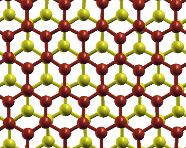
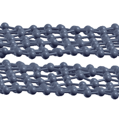
Figure 1: Top (upper) and side (lower) views of an atomic configuration of bilayer graphene obtained from MD simulations at $T$ = 800 K. In the top view, red and yellow spheres represent carbon atoms in the upper and lower graphene sheets, respectively.

The configuration space has been sampled for $T$ in the range from 50 to 1200 K. Given a temperature, a typical run consisted of $2\times 10^{5}$ MD steps for system equilibration and $8\times 10^{6}$ steps for calculation of ensemble averages. In Fig. 1 we show top and side views of an atomic configuration of bilayer graphene obtained in MD simulations at $T=800$ K. In the top view, red and yellow balls stand for carbon atoms in the upper and lower graphene layers in AB stacking pattern. In the side view, one can see atomic displacements in the out-of-plane direction, clearly observable at this temperature.

To characterize the elastic properties of bilayer graphene we consider uniaxial stress along the $x$ or $y$ directions, i.e., $\tau_{xx}\neq 0$ or $\tau_{yy}\neq 0$, as well as 2D hydrostatic pressure $P$ (biaxial stress) Behroozi (1996), which corresponds to $\tau_{xx}=\tau_{yy}=-P$, $\tau_{xy}=0$. Note that $P>0$ and $P<0$ mean compressive and tensile stress, respectively.

For comparison with our results for graphene bilayers, we also performed some MD simulations of graphite using the same potential LCBOPII. In this case we considered cells containing $4N$ carbon atoms (four graphene sheets), and periodic boundary conditions were assumed in the three space directions.

Other interatomic potentials have been used in last years to analyze several properties of graphene, in particular the so-called AIREBO potential Sfyris et al. (2015); Memarian et al. (2015); Zou et al. (2016); Anastasi et al. (2016); Ghasemi and Rajabpour (2017). Both LCBOPII and AIREBO models give very similar values for the equilibrium C–C interatomic distance and for the thermal expansion coefficient Memarian et al. (2015); Ghasemi and Rajabpour (2017); Herrero and Ramírez (2016). For the Young’s modulus of graphene, we find that the result obtained by employing the LCBOPII potential is closer to those yielded by ab initio calculations Memarian et al. (2015).

III Phonon dispersion bands and elastic constants at $T=0$

The elastic stiffness constants, $c_{ij}$, of bilayer graphene calculated with the LCBOPII potential model in the limit $T\rightarrow 0$ can be used as reference values for the finite-temperature analysis presented below. These elastic constants are calculated here from the harmonic dispersion relation of acoustic phonons. The interatomic force constants utilized to obtain the dynamical matrix were obtained by numerical differentiation of the forces using atom displacements of $1.5\times 10^{-3}$ Å with respect to the equilibrium (minimum-energy) positions.

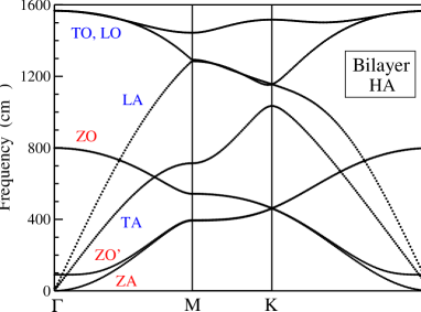
Figure 2: Phonon dispersion bands of bilayer graphene, obtained from diagonalization of the dynamical matrix for the LCBOPII potential model.

The phonon dispersion of bilayer graphene, calculated by diagonalization of the dynamical matrix is presented in Fig. 2 along high-symmetry directions of the 2D Brillouin zone. One finds 12 phonon bands, corresponding to four C atoms (2 per layer) in the crystallographic unit cell. Labels indicate the common names of the phonon bands: eight branches with in-plane atomic motion (LA, TA, LO, and TO, all of them two-fold degenerate), and four branches with displacements along the out-of-plane direction (ZA, ZO’, and a two-fold degenerate ZO band). The phonon dispersion presented in Fig. 2 is analogous to those obtained for other empirical potentials and DFT calculations Yan et al. (2008); Karssemeijer and Fasolino (2011); Koukaras et al. (2015); Singh and Hennig (2013). We emphasize the presence of the flexural ZA band, which is parabolic close to the $\Gamma$ point ($\omega\sim k^{2}$), and typically appears in 2D materials Wirtz and Rubio (2004); Amorim and Guinea (2013); Ramírez and Herrero (2019); Herrero and Ramírez (2021). Here $k$ denotes the wavenumber, i.e., $k=|{\bf k}|$, and ${\bf k}=(k_{x},k_{y})$ is a wavevector in the 2D hexagonal Brillouin zone.

Note also the presence of the optical mode ZO’, which does not appear in monolayer graphene, and in the case of the bilayer corresponds to the layer-breathing Raman-active $A_{2g}$ mode, for which a frequency of 89 cm^-1 has been measured Lin et al. (2018). The LCBOPII potential yields for this band at the $\Gamma$ point ($k=0$) a frequency of 92 cm^-1. This value is close to that found from ab initio calculations for graphene bilayers Yan et al. (2008).

The interatomic potential LCBOPII was used before to calculate the phonon dispersion bands of graphene and graphite Karssemeijer and Fasolino (2011). However, the version of the potential employed in Ref. Karssemeijer and Fasolino (2011) was somewhat different from that considered here, which gives a description of the graphene bending closer to experimental results Lambin (2014); Ramírez et al. (2016) (see Appendix A.1).

The sound velocities for the acoustic bands LA and TA along the direction $\Gamma\mathrm{M}$, with wavevectors $(k_{x},0,0)$, are given by the slope $\left(\partial\omega/\partial k_{x}\right)_{\Gamma}$ in the limit $k_{x}\to 0$. The elastic stiffness constants can be obtained from these velocities by using the following expressions, valid for the hexagonal symmetry of graphene Newnham (2005):

$$c_{11}=\rho\left(\frac{\partial\omega_{\rm LA}}{\partial k_{x}}\right)^{2}_{\Gamma}\;,$$ (1)

$$c_{12}=c_{11}-2\rho\left(\frac{\partial\omega_{\rm TA}}{\partial k_{x}}\right)^{2}_{\Gamma}\;.$$ (2)

where $\rho$ is the surface mass density of graphene. We find $c_{11}$ = 20.94 eV Å^-2 and $c_{12}$ = 4.54 eV Å^-2. Note that the dimensions of these elastic constants (force/length) coincide with those of the in-plane stress. These $c_{ij}$ can be converted into elastic constants $C_{ij}$ (units of force per square length), typical of three-dimensional (3D) materials, as $C_{ij}=c_{ij}/d_{0}$, using the interlayer distance $d_{0}$ of the minimum-energy configuration of bilayer graphene. Taking $d_{0}=3.3372$ Å, we find for the bilayer $C_{11}$ = 1005 GPa and $C_{12}$ = 218 GPa, near the values found for graphite in the classical low-$T$ limit, using the LCBOPII potential: 1007 and 216 GPa, respectively Herrero and Ramírez (2021).

IV Structural properties

IV.1 Interatomic distance

For bilayer graphene, the minimum-energy configuration for the LCBOPII potential corresponds to planar sheets and the interatomic distance between nearest neighbors in a layer amounts to 1.4193 Å. This distance turns out to be a little smaller than that found for monolayer graphene using the same interatomic potential ($r_{0}$ = 1.4199 Å). This fact was noticed by Zakharchenko et al. Zakharchenko et al. (2010) in their results of Monte Carlo simulations of graphene bilayers.

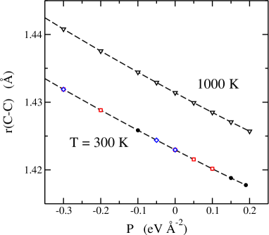
Figure 3: Interatomic distance vs 2D hydrostatic pressure for several cell sizes at $T$ = 300 and 1000 K. Data points are derived from MD simulations. For $T$ = 300 K, the data correspond to cell sizes: $N$ = 240 (solid circles), 448 (open squares), and 3840 (open diamonds). Open triangles correspond to $N$ = 240 at 1000 K. Error bars are less than the symbol size.

We have studied the change of the interatomic C–C distance $r$ (actual distance in 3D space) as a function of 2D hydrostatic pressure, $P$, at several temperatures. In Fig. 3 we present the dependence of $r$ on $P$ at $T$ = 300 and 1000 K. For $T$ = 300 K, data derived from MD simulations are shown for three cell sizes : $N$ = 240 (solid circles), 448 (open squares), and 3840 (open diamonds). We observe that the size effect on the interatomic distance is negligible, since differences between the results for different cell sizes are much smaller than the symbol size in Fig. 3. The data for $T$ = 1000 K (open triangles) correspond to $N$ = 240. Note that 2D hydrostatic pressure $P>0$ corresponds to compressive stress.

Close to $P=0$, this dependence can be fitted for $T$ = 300 K to an expression $r=r_{m}+\mu P$, where $r_{m}$ = 1.4230 Å is the interatomic distance for the stress-free bilayer at this temperature and $\mu=-0.0289$ ų/eV. For $T$ = 1000 K, we find $r_{m}$ = 1.4314 Å and $\mu=-0.0302$ Å³/eV. This slope is slightly larger than that found for $T$ = 300 K.

In connection with the interatomic distance $r$, we note that for a strictly planar geometry, the area per atom for an ideal honeycomb pattern is given by $S_{p}=3\sqrt{3}\,r^{2}/4$. At finite temperatures, however, the graphene layers are not totally planar and the actual in-plane area per atom is smaller than that given by the above expression, using the mean interatomic distance between nearest-neighbor C atoms. This is related with the so-called excess area and is discussed below in Sec. V.

In each hexagonal ring, two C–C bonds are aligned parallel to the $y$ direction (vertical in Fig. 1, top image), and the four other bonds form an angle of 30 degrees with the $x$ axis (horizontal direction). A compressive uniaxial stress along the $y$ axis ($\tau_{yy}<0$) causes a decrease in the length of the former bonds and an increase in the latter, as corresponds to a positive Poisson’s ratio. The opposite happens for $\tau_{xx}<0$.

IV.2 Interlayer spacing

For the minimum-energy configuration we find an interlayer distance $d_{0}=3.3372$ Å, to be compared with a distance of 3.3371 Å obtained in Ref. Zakharchenko et al. (2010) using an earlier version of the LCBOPII potential. At $T$ = 300 K we obtain $d$ = 3.374 Å, i.e., the interlayer distance increases somewhat due to bending of the graphene sheets caused by thermal motion.

The interlayer spacing is reduced in the presence of a tensile 2D hydrostatic pressure. Thus, for $P=-0.5$ eV/Ų and $T$ = 300 K, we find $d$ = 3.367 Å. This decrease is due to a reduction in the out-of-plane fluctuations under a tensile stress. The effect of this relatively high stress on the distance $d$ is, however, smaller than the thermal expansion up to 300 K. In the presence of a compressive stress in the $xy$ plane, one has an expansion of the interlayer spacing, but this kind of stress causes an instability of the bilayer configuration for relatively small values of $P$, as explained below.

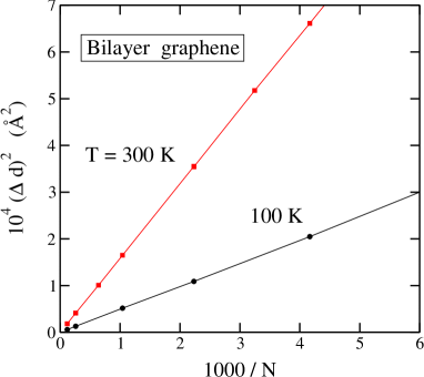
Figure 4: MSF of the interlayer distance as a function of the inverse cell size for $T$ = 100 K (circles) and 300 K (squares), as derived from MD simulations of bilayer graphene.

The mean-square fluctuation (MSF) of the interlayer distance, $(\Delta d)^{2}=\langle d^{2}\rangle-\langle d\rangle^{2}$, associated to thermal motion at finite temperatures, is related to the interaction between graphene layers. This MSF is expected to depend on the size of the considered simulation cell, and becomes negligible in the thermodynamic limit ($N\to\infty$). In Fig. 4 we display $(\Delta d)^{2}$ derived from our MD simulations as a function of the inverse cell size for stress-free bilayer graphene at $T=100$ K (circles) and 300 K (squares). One observes that $(\Delta d)^{2}\to 0$ for $1/N\to 0$, and grows linearly for increasing inverse cell size.

To connect these results with the energetics of bilayer graphene, we have calculated the interlayer interaction energy for several values of the spacing $d$ near the distance $d_{0}$ corresponding to the minimum-energy configuration. The interaction energy per atom can be written as:

$$E_{\rm int}=E_{\rm int}^{0}+\frac{1}{2}k(d-d_{0})^{2}\,.$$ (3)

where $E_{\rm int}^{0}$ is the energy for distance $d_{0}$, and $k$ is an effective interaction constant which is found to amount to 0.093 eV/Ų. Then, for the whole simulation cell ($2N$ atoms in a bilayer), the energy corresponding to a distance $d$ close to $d_{0}$ is

$$\bar{E}_{\rm int}=\bar{E}_{\rm int}^{0}+kN(d-d_{0})^{2}\,.$$ (4)

Thus, thermal motion at temperature $T$, associated to the degree of freedom $d$, will cause a MSF of this variable, $(\Delta d)^{2}$, given by the mean potential energy:

$$kN(\Delta d)^{2}=\frac{1}{2}k_{B}T\,,$$ (5)

where $k_{B}$ is Boltzmann’s constant. This means that for a given temperature, $(\Delta d)^{2}$ scales as $1/N$, as shown in Fig. 4.

As indicated in Sec. III, the phonon spectra of monolayer and bilayer graphene are similar. The main difference between them is the appearance in the latter of the ZO’ vibrational band, which is almost flat in a region of ${\bf k}$-space near the $\Gamma$ point (see Fig. 2). As noted above, this vibrational mode of bilayer graphene is the layer-breathing Raman-active $A_{2g}$ mode Lin et al. (2018). The frequency of the ZO’ band at $\Gamma$ (which will be denoted here $\omega_{0}$) can be related to the interlayer coupling constant $k$ as $\omega_{0}=(k_{N}/M_{\rm red})^{1/2}$, with $k_{N}=2Nk$ and the reduced mass $M_{\rm red}=Nm/2$ ($m$: atomic mass of carbon). We find $\omega_{0}=2(k/m)^{1/2}$. and putting for the coupling constant $k$ = 0.093 eV Å^-2/atom, one obtains $\omega_{0}=$ 92 cm^-1, which coincides with the frequency of the ZO’ band derived from the dynamical matrix at the $\Gamma$ point. Michel and Verberck Michel and Verberck (2008) have studied the evolution of this frequency $\omega_{0}$ with the number of sheets $n$ in graphene multilayers. They found an increase of $\omega_{0}$ for rising $n$, which saturates to a value of 127 cm^-1 for large $n$ (graphite).

The interlayer coupling in bilayer graphene was studied before by Zakharchenko et al. Zakharchenko et al. (2010) by means of Monte Carlo simulations. The low-frequency part of the ZO’ band was described by these authors using a parameter $\gamma$, which is related to the parameters employed here as $\gamma=\rho\,\omega_{0}^{2}/4$, where $\rho$ is the surface mass density. From this expression we find $\gamma$ = 0.035 eV Å^-4, which agrees with the low-temperature result derived from Monte Carlo simulations (Fig. 7 in Ref. Zakharchenko et al. (2010)).

Fluctuations in the interlayer spacing of bilayer graphene at temperature $T$ are related with the isothermal compressibility in the out-of-plane direction, $\chi_{z}$ Herrero and Ramírez (2019). In fact, $\chi_{z}$ can be calculated from the MSF $(\Delta d)^{2}$ by using the expression Herrero and Ramírez (2019)

$$\chi_{z}=\frac{L_{x}L_{y}}{k_{B}T}\frac{(\Delta d)^{2}}{\langle d\rangle}\,.$$ (6)

Using $(\Delta d)^{2}=1.65\times 10^{-4}$ Å² for $N$ = 960 at $T$ = 300 K, we find $\chi_{z}=2.96\times 10^{-2}$ GPa^-1. This value is a little larger than experimental results for graphite, of about $2.7\times 10^{-2}$ GPa^-1 Blakslee et al. (1970); Nicklow et al. (1972). This is consistent with the fact that bilayer graphene is more compressible than graphite in the $z$ direction, since in the latter each layer is surrounded by two other graphene layers, whereas in the former each sheet has a single neighbor.

IV.3 Out-of-plane motion

The minimum-energy configuration for the graphene layers, i.e., the classical low-temperature limit, corresponds to planar sheets. At finite temperatures the graphene sheets are bent. This bending is directly related to the atomic motion in the out-of-plane $z$ direction, whose largest vibrational amplitudes come from low-frequency ZA modes with long wavelength (small $k$). For stress-free graphene, the ZA phonon branch can be described close to the $\Gamma$ point by a parabolic dispersion relation of the form $\omega({\bf k})=\sqrt{\kappa/\rho}\,k^{2}$, with the bending constant $\kappa$ = 1.49 eV (see Fig. 2).

It is known that the atomic MSF in the $xy$ layer plane is relatively insensitive to the system size, but the out-of-plane MSF has important finite size effects. This dependence on $N$ has been studied earlier for stress-free monolayer and bilayer graphene by means of Monte Carlo and molecular dynamics simulations, in particular using the LCBOPII interatomic potential Herrero and Ramírez (2016). For system size $N$, one has an effective cut-off for the wavelength $\lambda$ given by $\lambda_{\rm max}\approx L$, where $L=(NS_{p})^{1/2}$, and $S_{p}$ is the in-plane area per atom. Thus, the minimum wavenumber present for size $N$ is $k_{\rm min}=2\pi/\lambda_{\rm max}$, and the minimum frequency for ZA modes is

$$\omega_{\rm min}\approx\frac{4\pi^{2}}{NS_{p}}\,\left(\frac{\kappa}{\rho}\right)^{\frac{1}{2}}\;,$$ (7)

so that $\omega_{\rm min}$ scales as $N^{-1}$.

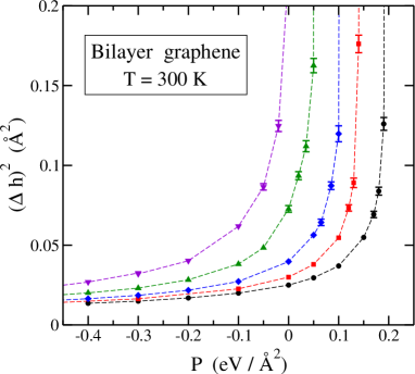
Figure 5: Atomic MSF in the $z$ direction vs 2D hydrostatic pressure for several cell sizes at $T$ = 300 K. From left to right: $N$ = 3840 (triangles down), 960 (triangles up), 448 (diamonds), 308 (squares), and 240 (circles). Positive (negative) $P$ means compressive (tensile) stress. Dashed lines are guides to the eye.

For a graphene sheet, we call ${\bf r}\equiv(x,y)$ the 2D position on the layer plane and $h({\bf r})$ is the distance to the mean plane of the sheet. In Fig. 5 we present the MSF of the atomic positions in the $z$ direction for bilayer graphene, $(\Delta h)^{2}=\langle h^{2}\rangle-\langle h\rangle^{2}$, as a function of 2D hydrostatic pressure $P$ for various cell sizes at $T$ = 300 K. Symbols represent results derived from our MD simulations, with cell size decreasing from left to right: $N$ = 3840, 960, 448, 308, and 240. One observes first that $(\Delta h)^{2}$ appreciably increases for rising system size, as expected from earlier studies of 2D materials Gao and Huang (2014). For the largest size displayed in Fig. 5, $N=3840$, we find at $P=0$, $(\Delta h)^{2}$ = $0.22\pm 0.01$ Ų (not shown in the figure). The dependence of $(\Delta h)^{2}$ on $N$ for stress-free bilayer graphene will be analyzed below in Sec. VII. Second, we also observe in Fig. 5 that the difference in atomic MSF between different system sizes is reduced for increasing tensile stress ($P<0$). $(\Delta h)^{2}$ grows as the tensile stress is reduced ($d(\Delta h)^{2}/dP>0$), and eventually diverges at a size-dependent critical pressure $P_{c}(N)>0$. Third, one sees that $P_{c}(N)$ approaches zero for rising system size.

The dependence of the critical pressure $P_{c}$ on $N$ will be discussed below in relation to fluctuations of the in-plane area $S_{p}$, which are also found to diverge in parallel with $(\Delta h)^{2}$ for each size $N$. The origin of this instability is related to the appearance of imaginary frequencies for vibrational modes in the ZA flexural band for pressure $P_{c}(N)$. This will be discussed in Sec. VI in connection with the 2D modulus of hydrostatic compression $B_{p}$, which is found to vanish at $P_{c}$.

V In-plane and excess area

The in-plane area, $S_{p}=L_{x}L_{y}/N$, is the variable conjugate to the pressure $P$ in the isothermal-isobaric ensemble considered here. Its temperature dependence, $S_{p}(T)$, has been analyzed earlier in detail for monolayer and bilayer graphene from atomistic simulations Zakharchenko et al. (2010); Herrero and Ramírez (2016, 2019). For the bilayer we find in the minimum-energy configuration (T = 0) an area $S_{0}$ = 2.6169 Ų/atom, in agreement with earlier calculations Zakharchenko et al. (2010); Herrero and Ramírez (2019). Here, we discuss the behavior of $S_{p}$ as a function of 2D hydrostatic stress, both tensile and compressive.

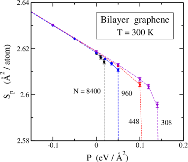
Figure 6: In-plane area per atom vs 2D hydrostatic pressure $P$ at $T$ = 300 K. Shown are results for cell sizes $N$ = 308 (traingles), 448 (squares), 960 (diamonds), and 8400 (circles). Error bars, when not displayed, are in the order of the symbol size. Dashed lines are guides to the eye.

In Fig. 6 we display the dependence of $S_{p}$ on $P$ for several cell sizes at $T$ = 300 K. We present data for $N$ = 308, 448, 960, and 8400. For tensile stress $P<-0.05$ eV/Ų, $S_{p}$ data for different cell sizes are indistinguishable at the scale of Fig. 6. In fact, we obtain a nearly linear dependence with a slope $dS_{p}/dP\approx-0.12$ Å⁴/eV. However, differences appear close to $P=0$, and even more for compressive stress ($P>0$). For each size $N$, one observes a fast decrease in $S_{p}$ close to the corresponding stability limit of the planar phase. We obtain values of the in-plane area below 2.58 Ų/atom, not shown in the figure for clarity. Changes in $S_{p}$ correspond to linear strain $\epsilon_{L}$ as: $S_{p}=S_{0}(1+\epsilon_{L})^{2}$. This means that the vertical range in Fig. 6 corresponds to a strain range between $\epsilon_{L}=-7.1\times 10^{-3}$ (compression) and $4.4\times 10^{-3}$ (tension).

In our MD simulations, carbon atoms are free to move in the out-of-plane direction ($z$ coordinate), and the real surface of a graphene sheet is not strictly planar, having an actual area larger than the area of the simulation cell in the $xy$ plane. Differences between the in-plane area $S_{p}$ and real area $S_{r}$ were considered earlier in the context of biological membranes Imparato (2006); Waheed and Edholm (2009); Chacón et al. (2015) and in recent years for graphene, as a paradigmatic crystalline membrane Ramírez and Herrero (2017); Nicholl et al. (2017). An explicit differentiation between both areas is relevant to understand certain properties of 2D materials Safran (1994). Some experimental techniques can be sensitive to properties connected to the area $S_{r}$, whereas other methods may be suitable to analyze variables related to the area $S_{p}$ Nicholl et al. (2015, 2017).

Here we calculate the real area $S_{r}$ of both sheets in bilayer graphene by a triangulation method based on the atomic positions along the simulation runs Ramírez and Herrero (2017); Herrero and Ramírez (2019). In the sequel, $S_{r}$ will denote the real area per atom. The difference $S_{r}-S_{p}$ has been called in the literature hidden area Nicholl et al. (2017) or excess area Helfrich and Servuss (1984); Fournier and Barbetta (2008). We consider the dimensionless excess area $\Phi$ for a graphene sheet, defined as Helfrich and Servuss (1984); Fournier and Barbetta (2008)

$$\Phi=\frac{S_{r}-S_{p}}{S_{p}}\;.$$ (8)

In the classical low-temperature limit, $\Phi$ vanishes, as the sheets become strictly planar for $T\to 0$. We note that this is not the case in a quantum calculation, where one has $\Phi>0$ for $T\to 0$ due to atomic zero-point motion Herrero and Ramírez (2018a).

The excess area is related to the amplitude of the vibrational modes in the $z$ direction. This allows one to find analytical expressions for $\Phi$ in terms of the frequency of those modes. The instantaneous real area $S_{r}^{*}$ may be expressed in a continuum approximation as Imparato (2006); Waheed and Edholm (2009); Ramírez and Herrero (2017)

$$S_{r}^{*}=\frac{1}{N}\int_{0}^{L_{x}}\int_{0}^{L_{y}}dx\,dy\,\sqrt{1+|\nabla h({\bf r})|^{2}}\;,$$ (9)

where $h({\bf r})$ represents the distance to the mean $xy$ plane of the sheet, as in Sec. IV.C. Expanding $h({\bf r})$ as a Fourier series with wavevectors ${\bf k}=(k_{x},k_{y})$ in the 2D hexagonal Brillouin zone, the real area $S_{r}=\langle S_{r}^{*}\rangle$ may written as Safran (1994); Chacón et al. (2015); Ramírez and Herrero (2017)

$$S_{r}=S_{p}\left[1+\frac{1}{2N}\sum_{\bf k}k^{2}\langle|H({\bf k})|^{2}\rangle\right]\;,$$ (10)

where $H({\bf k})$ are the Fourier components of $h({\bf r})$ (see Appendix B). Taking into account that the MSF of a mode with frequency $\omega_{j}({\bf k})$ is given by $k_{B}T/m\omega_{j}({\bf k})^{2}$, $m$ being the atomic mass of carbon, one finds for the excess area

$$\Phi=\frac{k_{B}T}{2mN}\sum_{j,{\bf k}}\frac{k^{2}}{\omega_{j}({\bf k})^{2}}\;,$$ (11)

where the sum in $j$ is extended to phonon branches with atomic motion in the $z$ direction, i.e., ZA, ZO, and ZO’.

For small $k$, the contribution of ZO and ZO’ modes to the sum in Eq. (11) vanishes for $k\to 0$, as in both cases $\omega_{j}({\bf k})$ converges to positive values. For the flexural ZA band with negligible effective stress, we have $\omega_{\rm ZA}({\bf k})\propto k^{2}$, and $k^{2}/\omega_{\rm ZA}({\bf k})^{2}\propto k^{-2}$, so that the contribution of ZA modes with small $k$ is dominant in the sum in Eq. (11). The minimum wavenumber $k_{\rm min}$ available for cell size $N$ scales as $k_{\rm min}\sim N^{-1/2}$ (see Sec. IV.C). Thus, its contribution to $\Phi$ grows linearly with $N$, and diverges for stress-free graphene in the thermodynamic limit. This divergence disappears in the presence of a tensile in-plane stress (even small), be it caused by internal tension or by an external pressure.

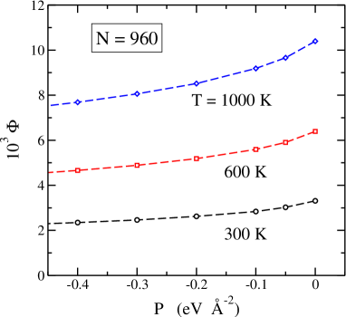
Figure 7: Excess area per atom vs 2D hydrostatic pressure $P$ for cell size $N$ = 960 at $T$ = 300 K (circles), 600 K (squares), and 1000 K (diamonds). Open symbols are data points derived from MD simulations of bilayer graphene. Dashed lines are guides to the eye.

In Fig. 7 we display $\Phi$ for bilayer graphene as a function of 2D hydrostatic pressure $P$. Symbols represent data derived from our MD simulations at three temperatures: $T$ = 300 K (circles), 600 K (squares), and 1000 K (diamonds). Dashed lines are guides to the eye. These data were obtained for system size $N=960$. The excess area $\Phi$ increases as $T$ is raised, in agreement with the growing amplitude of the out-of-plane vibrational modes (see Eq.  (11)). In fact, a classical harmonic approximation (HA) for the vibrational modes predicts a linear increase of $\Phi$ with temperature. From the results shown in Fig. 7 for $P=0$, we find the ratios $\Phi$(1000 K)/$\Phi$(300 K) = 3.14 and $\Phi$(600 K)/$\Phi$(300 K) = 1.93, a little less than the corresponding temperature ratios (3.33 and 2.0). For a pressure $P=-0.5$ eV/Ų, we find for those ratios at the same temperatures values of 3.28 and 1.99, respectively, closer to the harmonic expectancy. An in-plane tensile stress causes a decrease in the vibrational amplitudes in the $z$ direction, and then the modes are better described by a harmonic approach.

VI Elastic constants and compressibility at finite temperatures

VI.1 Temperature dependence

Using MD simulations one can gain insight into the elastic properties of materials under different kinds of applied stresses, e.g., hydrostatic or uniaxial. In particular, we consider elastic stiffness constants, $c_{ij}$, and compliance constants, $s_{ij}$, for 2D crystalline materials with hexagonal structure such as graphene. We call $\tau_{ij}$ and $e_{ij}$ the components of the stress and strain tensors, respectively. $\tau_{ij}$ is the force per unit length parallel to direction $i$, acting in the $xy$ plane on a line perpendicular to the $j$ direction. We use the standard notation for strain components, with $e_{ij}=\epsilon_{ij}$ for $i=j$, and $e_{ij}=2\epsilon_{ij}$ for $i\neq j$ Ashcroft and Mermin (1976); Marsden et al. (2018). More details on elastic properties of 2D crystals can be found in Ref. Behroozi (1996).

In terms of the compliance constants, we have for applied stress $\{\tau_{ij}\}$:

$$\begin{pmatrix}e_{xx}\cr e_{yy}\cr e_{xy}\end{pmatrix}=\begin{pmatrix}s_{11}&s_{12}&0\cr s_{12}&s_{11}&0\cr 0&0&2(s_{11}-s_{12})\end{pmatrix}\begin{pmatrix}\tau_{xx}\cr\tau_{yy}\cr\tau_{xy}\end{pmatrix}\;.$$ (12)

The matrix of stiffness constants $\{c_{ij}\}$ is the inverse of $\{s_{ij}\}$, so that we have the relations

$$c_{11} = \frac{s_{11}}{s_{11}^{2}-s_{12}^{2}}\;,$$ (13)

$$c_{12} = \frac{s_{12}}{s_{12}^{2}-s_{11}^{2}}\;.$$ (14)

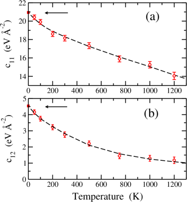
Figure 8: Temperature dependence of the elastic stiffness constants of bilayer graphene, as derived from MD simulations for $N$ = 960 (open circles): (a) $c_{11}$, (b) $c_{12}$. Dashed lines are guides to the eye. Solid squares at $T=0$, indicated by arrows, show the values of $c_{11}$ and $c_{12}$ derived from the HA using Eqs. (1) and (2).

In Fig. 8 we present the stiffness constants as a function of temperature, as derived from our MD simulations of bilayer graphene, using Eq. (12) (open circles). Panels (a) and (b) show results for $c_{11}$ and $c_{12}$, respectively. Solid squares at $T$ = 0, signaled by arrows, indicate results for $c_{11}$ and $c_{12}$ obtained from the phonon dispersion bands as indicated in Sec. II, using Eqs. (1) and (2). We find that finite-temperature data for the stiffness constants converge at low $T$ to the results of the HA for both $c_{11}$ and $c_{12}$. For rising temperature, the stiffness constants decrease rather fast. This decrease is especially large for $c_{12}$, which is found to be 1.18 eV/Ų at $T$ = 1200 K vs the classical low-$T$ limit of 4.54 eV/Ų.

Comparing the elastic constants $c_{11}$ and $c_{12}$ found here for bilayer graphene with those corresponding to monolayer graphene Herrero and Ramírez (2017) and graphite Herrero and Ramírez (2021) (normalized to one layer), we find that they increase for the sequence monolayer-bilayer-graphite. This agrees with the fact that interaction between layers reduces the amplitude of out-of-plane vibrational modes, thus favoring an increase in the “hardness” of the layers. This trend is similar to that discussed below for the 2D compression modulus $B_{p}$.

The Poisson’s ratio $\nu$ can be obtained as the quotient $c_{12}/c_{11}$. This yields for $T=0$ (HA) $\nu=0.22$. From the results of our simulations, we find $\nu$ = 0.15 and 0.09 for $T$ = 300 and 1000 K, respectively, with an important reduction for rising $T$, as a consequence of the decrease in $c_{12}$. Calculations based on the self-consistent screening approximation Le Doussal and Radzihovsky (1992); Kosmrlj and Nelson (2013); Le Doussal and Radzihovsky (2018) (SCSA) predict for $P=0$ in the thermodynamic limit ($N\to\infty$) a Poisson’s ratio $\nu=-1/3$. A negative value for this ratio is also expected from the calculations presented by Burmistrov et al. Burmistrov et al. (2018) for $N\to\infty$. From the results of our MD simulations, we do not find, however, any indication for a negative Poisson’s ratio in the parameter region considered here. This is in line with earlier results of Monte Carlo simulations by Los et al. Los et al. (2016) for monolayer graphene in a region of system sizes larger than those considered here for bilayer graphene.

The 2D modulus of hydrostatic compression $B_{p}$ is defined for layered materials at temperature $T$ as Behroozi (1996)

$$B_{p}=-\frac{S_{p}}{n}\left(\frac{\partial P}{\partial S_{p}}\right)_{T}\,.$$ (15)

Note the factor $n$ (number of sheets) in the denominator, i.e., $B_{p}$ is the compression modulus per layer. $P$ and $S_{p}$ appearing on the r.h.s. of Eq. (15) are variables associated to the layer plane, and in fact the pressure in the isothermal-isobaric ensemble used here is the conjugate variable to the area $S_{p}$.

One can also calculate the modulus $B_{p}$ on the basis of the fluctuation formula Landau and Lifshitz (1980); Ramírez and Herrero (2017); Herrero and Ramírez (2018b)

$$B_{p}=\frac{k_{B}TS_{p}}{nN(\Delta S_{p})^{2}}\;,$$ (16)

where $(\Delta S_{p})^{2}$ is the mean-square fluctuation of the area $S_{p}$, which is calculated here from MD simulations at $P=0$. This formula provides us with a practical procedure to obtain $B_{p}$, vs calculating the derivative $(\partial S_{p}/\partial P)_{T}$ by numerical methods, which requires additional MD simulations at hydrostatic pressures close to $P=0$. For some temperatures we have verified that results for $B_{p}$ found with both procedures coincide within statistical error bars, which is a consistency check for our results.

The modulus $B_{p}$ can be also obtained from the elastic constants of bilayer graphene. Taking into account Eq. (12), the change of the in-plane area, $\Delta S_{p}$ due to a 2D hydrostatic pressure $P$, is given by

$$\frac{\Delta S_{p}}{S_{p}}=e_{xx}+e_{yy}=-2(s_{11}+s_{12})P\;.$$ (17)

Combining Eqs. (15) and (17), one finds

$$B_{p}=\frac{1}{2(s_{11}+s_{12})}\;,$$ (18)

which can be also written as $B_{p}=(c_{11}+c_{12})/2$. These expressions are valid for 2D materials with hexagonal symmetry.

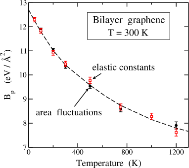
Figure 9: 2D modulus of hydrostatic compression, $B_{p}$, as a function of temperature for stress-free bilayer graphene ($P$ = 0) and $N$ = 960. Solid circles represent results derived from fluctuations of the in-plane area, using Eq. (16). Open squares are data points obtained from the elastic constants $s_{11}$ and $s_{12}$. The dashed line is a guide to the eye.

In Fig. 9 we present the modulus $B_{p}$ of bilayer graphene as a function of $T$, as derived from our MD simulations. Solid circles represent results obtained from the in-plane area fluctuation $(\Delta S_{p})^{2}$ by employing Eq. (16). Open squares are data points calculated from the elastic constants. Both sets of results coincide within error bars. At low temperature, $B_{p}$ converges to the value given by the expression

$$B_{0}=\frac{S_{p}}{n}\frac{\partial^{2}E}{\partial S_{p}^{2}}\;,$$ (19)

where $E$ is the energy. For bilayer graphene we have $B_{0}$ = 12.74 eV/Ų, which agrees with the extrapolation of finite-$T$ results to $T=0$. The modulus $B_{p}$ derived from MD simulations is found to decrease fast as the temperature is raised, and at $T$ = 1200 K it amounts to about 60% of the low-$T$ limit $B_{0}$.

For monolayer graphene, the same interatomic potential yields in a HA: $B_{0}$ = 12.65 eV/Ų, somewhat less than the value found for the bilayer. This difference is larger at finite temperatures. Even though interlayer interactions are relatively weak, they give rise to a reduction in the vibrational amplitudes of out-of-plane modes, and as a result the graphene sheets become “harder” in the bilayer, so that the modulus $B_{p}$ increases with respect to an isolated sheet. Moreover, the difference between the modulus $B_{p}$ per sheet for bilayer and monolayer graphene grows for rising system size $N$ (see Sec. VII).

The in-plane Young’s modulus $E_{p}$ can be obtained from $B_{p}$ through the expression $E_{p}=2B_{p}(1-\nu)$. This yields for the bilayer at $T=0$, $E_{p}$ = 19.87 eV/Ų, which translated into units of force per square length gives $E_{p}/d=$ 0.954 TPa, similar to values appearing in the literature Memarian et al. (2015); Cao et al. (2018).

VI.2 Mechanical instability under stress

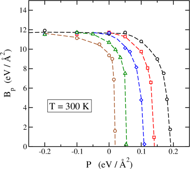
Figure 10: Modulus $B_{p}$ as a function of 2D hydrostatic pressure at $T$ = 300 K, for various cell sizes. Symbols are data points derived from MD simulations for various cell sizes. From left to right: $N$ = 8400, 960, 448, 308, and 240. Dashed lines are guides to the eye.

The modulus $B_{p}$ is particularly interesting to study the critical behavior of bilayer graphene under 2D hydrostatic pressure. In Fig. 10 we present the dependence of $B_{p}$ on $P$, including tensile and compressive stresses. Symbols represent values derived from MD simulations for various cell sizes. From left to right: $N$ = 8400, 960, 448, 308, and 240. For each size $N$, increasing in-plane compression causes a fast decrease in $B_{p}$, which vanishes for a pressure $P_{c}(N)$, where the bilayer graphene with planar sheets becomes mechanically unstable. This is typical of a spinodal point in the $(P,T)$ phase diagram Sciortino et al. (1995); Herrero (2003); Ramírez and Herrero (2018a); Callen (1985). For $P>P_{c}$, the stable configuration corresponds to wrinkled graphene sheets, as observed earlier for monolayer graphene Ramírez and Herrero (2017).

For given $N$ and $T$, there is a pressure region (compressive stress) where bilayer graphene is metastable, i.e., for $P<P_{c}$. The spinodal line, which delineates the metastable phase from the unstable phase, is the locus of points $P_{c}(N,T)$ where $B_{p}=0$. This kind of spinodal lines have been studied earlier for water Speedy (1982), as well as for ice, SiO₂ cristobalite Sciortino et al. (1995), and noble-gas solids Herrero (2003) near their stability limits. In recent years, this question has been investigated for 2D materials, and in particular for monolayer graphene Ramírez and Herrero (2018a, 2020).

According to Eq. (16), vanishing of $B_{p}$ for finite $N$ corresponds to a divergence of the area fluctuation $(\Delta S_{p})^{2}$ to infinity. Moreover, the MSF of the atomic $z$ coordinate, $(\Delta h)^{2}$, diverges at the corresponding spinodal pressure, as mentioned in Sec. IV.C. For graphene bilayers, this spinodal instability is associated to a soft vibrational mode in the ZA branch. In fact, for each $N$ this instability appears for increasing $P$ when the frequency of the ZA vibrational mode with minimum wavenumber, $k_{\rm min}$, reaches zero ($\omega_{\rm min}\to 0$).

Close to a spinodal point, the modulus $B_{p}$ behaves as a function of $P$ as $B_{p}\sim(P_{c}-P)^{1/2}$ (see Appendix C). This pressure dependence agrees with the shape of the curves shown in Fig. 10 near the spinodal pressure $P_{c}$ for each size $N$. Note that $P_{c}$ moves to smaller compressive pressures as $N$ rises. This size effect is analyzed below in Sec. VII. We also note that, for a given size $N$, the critical stress $P_{c}$ depends on temperature, as shown before for monolayer graphene Ramírez and Herrero (2018b). It was found that $P_{c}$ increases for rising temperature, as a consequence of a raise in vibrational amplitudes in the out-of-plane direction. We have checked that something similar happens for bilayer graphene, but a detailed study of this question requires additional MD simulations, which will be the subject of future work.

VII Size effects

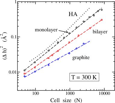
Figure 11: Atomic MSF in the $z$ direction vs cell size for $T$ = 300 K in a logarithmic plot. Data derived from MD simulations are given for monolayer graphene (circles), bilayer graphene (squares), and graphite (diamonds). Error bars are in the order of the symbol size. Dashed lines are least-square fits to the data points. The dotted line represents the MSF corresponding to a HA.

As noted above, some properties of 2D materials display important size effects. In this section, we concentrate on the size dependence of the MSF $(\Delta h)^{2}$, the modulus $B_{p}$, and the spinodal pressure $P_{c}$ for bilayer graphene, and study their asymptotic behavior for large $N$.

In Fig. 11 we present in a logarithmic plot the atomic MSF $(\Delta h)^{2}$ in the $z$ direction as a function of system size at $T$ = 300 K. Results derived from MD simulations for stress-free bilayer graphene are shown as open squares. For comparison we also display data for monolayer graphene (circles) and graphite (diamonds), obtained from MD simulations with the LCBOPII interatomic potential. For the system sizes presented in Fig. 11, $(\Delta h)^{2}$ may be expressed in the three cases as a power of $N$: $(\Delta h)^{2}\sim N^{\alpha}$. We find for the exponent $\alpha$ values of 0.78, 0.69, and 0.56 for monolayer, bilayer graphene, and graphite, respectively.

The MSF in the $z$ direction can be written in a HA as:

$$(\Delta h)^{2}=\frac{k_{B}T}{N\rho S_{p}}\sum_{j,{\bf k}}\frac{1}{\omega_{j}({\bf k})^{2}}\;,$$ (20)

where the sum in $j$ is extended to the phonon bands with atomic motion in the out-of-plane direction, i.e., ZA, ZO, and ZO’ for bilayer graphene (as above in Eq. (11)). The sum in Eq. (20) is dominated by ZA modes with wavevector close to the $\Gamma$ point, i.e. small frequency $\omega$. The inputs of bands ZO and ZO’ are almost independent of the system size, and they give a joint contribution of $\approx 8\times 10^{-3}$ Å² to $(\Delta h)^{2}$ in Eq. (20).

For the ZA band, putting a dispersion $\rho\,\omega^{2}=\kappa k^{4}$, one finds Gao and Huang (2014)

$$(\Delta h)^{2}_{\rm ZA}=\frac{C\,k_{B}TS_{p}N}{16\pi^{4}\,\kappa}\;,$$ (21)

where $C=6.03$ is a constant. Thus, in a HA the ZA band yields a contribution proportional to $N$ and an exponent $\alpha=1$. The result of the HA including the inputs of the three phonon bands ZA, ZO, and ZO’ is shown in Fig. 11 as a dotted line. For large $N$, $(\Delta h)^{2}$ is dominated by atomic displacements associated to ZA modes and we find that it increases linearly with $N$. For small $N$, one observes a departure from the linear trend due to contributions of ZO and ZO’ modes.

The size dependence of $(\Delta h)^{2}$ obtained from MD simulations for stress-free bilayer graphene can be understood assuming an effective dependence for the frequency of ZA modes as $\rho\,\omega^{2}=\bar{\kappa}\,k^{\beta}$, where $\bar{\kappa}$ is a modified bending constant and $\beta$ is an exponent controlling the frequency of long-wavelength (small frequency) modes. This expression assumes an effective shape for the ZA band at finite temperatures, as a consequence of anharmonicity in the vibrational modes, and is similar to that considered earlier for monolayer graphene Gao and Huang (2014); Tröster (2013); Los et al. (2016). Assuming such a dispersion for ZA modes in the bilayer, we have for large $N$:

$$(\Delta h)^{2}_{\rm eff}\approx\frac{k_{B}T}{\bar{\kappa}NS_{p}}\sum_{{\bf k}}\frac{1}{k^{\beta}}\;,$$ (22)

where the sum is extended to ${\bf k}$ points in the 2D Brillouin zone.

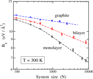
Figure 12: Modulus $B_{p}$ as a function of cell size $N$ at $T$ = 300 K on a logarithmic plot. Symbols represent data derived from MD simulations for a graphene monolayer (circles), bilayer (squares), and graphite (diamonds). Dashed lines are guides to the eye.

Taking into account the relation between the minimum wavenumber $k_{\rm min}$ and the size $N$, and replacing the sum in Eq. (22) by an integral, one finds a size dependence

$$(\Delta h)^{2}_{\rm eff}=\frac{D}{\bar{\kappa}}k_{B}T\,(S_{p}N)^{\frac{\beta}{2}-1}\;.$$ (23)

where $D$ is an integration constant. This means that our exponent $\alpha$ can be related to $\beta$ as $\alpha=\beta/2-1$, which yields for bilayer graphene $\beta$ = 3.38. Similar effective exponents can be derived from MD simulation results for monolayer graphene and graphite, for which we find $\beta$ = 3.56 and 3.12, respectively.

The 2D modulus of hydrostatic compression $B_{p}$ introduced in Sec. VI also displays finite-size effects. In Fig. 12 we show in a logarithmic plot the dependence of $B_{p}$ on $N$ at $T$ = 300 K. Open squares represent results obtained for bilayer graphene from MD simulations. For comparison, we also display data for monolayer graphene (circles), as well as for graphite (diamonds). For $N>500$, $B_{p}$ can be fitted for the bilayer to an expression $B_{p}\sim N^{-\zeta}$, with an exponent $\zeta=0.086$. From similar fits for monolayer graphene and graphite, we find the exponents 0.159 and 0.033, respectively. Note that the exponent $\zeta$ for the bilayer is about one half of that corresponding to the monolayer. This indicates that the size effect is less important for the former than for the latter, as visualized in Fig. 12.

Looking at Eq. (16), and taking into account that $S_{p}$ changes slowly with $N$, we have for the area fluctuation a size dependence: $(\Delta S_{p})^{2}\sim N^{\zeta-1}$. This means that $(\Delta S_{p})^{2}_{B}/(\Delta S_{p})^{2}_{M}\sim N^{-0.073}$, where the subscripts $B$ and $M$ refer to bilayer and monolayer, respectively. For small $N$, the area fluctuation is similar for bilayer and monolayer graphene, but they become comparatively smaller for the bilayer as the size increases. Our exponent for the monolayer can be translated to a dependence on the cell side length $B_{p}\sim L^{-2\zeta}$, with $2\zeta$ = 0.318, close to the exponent 0.323 found by Los et al. Los et al. (2016) for the dependence of $B_{p}$ on $L$.

The size dependence of the critical pressure $P_{c}$ introduced in Sec. VI is shown in Fig. 13, where we have plotted values of $P_{c}$ derived from MD simulations at $T$ = 300 K for several cell sizes. One observes at first sight a linear dependence of $P_{c}$ with the inverse cell size, $N^{-1}$. This dependence may be understood by considering the effect of a compressive stress on ZA vibrational modes, as follows.

For a single graphene layer under a 2D hydrostatic pressure $P$, the dispersion relation of ZA modes may be written as

$$\rho\,\omega^{2}=\sigma k^{2}+\kappa\,k^{4}$$ (24)

where $\sigma=-P$ Herrero and Ramírez (2017); Ramírez and Herrero (2018a). For increasing compressive stress, $\omega$ is reduced, i.e. $d\omega/dP<0$. Thus, for system size $N$, a graphene layer becomes unstable when the frequency of the ZA mode with wavenumber $k_{\rm min}$ vanishes. This occurs for

$$\sigma\,k_{\rm min}^{2}+\kappa\,k_{\rm min}^{4}=0\;,$$ (25)

which yields a critical stress

$$\sigma_{c}=-\kappa\,k_{\rm min}^{2}\;.$$ (26)

As indicated above, the minimum wavenumber $k$ present for cell size $N$ is $k_{\rm min}=2\pi/(NS_{p})^{1/2}$. For bilayer graphene, the in-plane critical pressure is given by $P_{c}=-2\sigma_{c}$, from where we have:

$$P_{c}\,N=\frac{8\,\pi^{2}\kappa}{S_{p}}\;.$$ (27)

Putting $\kappa$ = 1.49 eV and $S_{p}$ = 2.617 Ų/atom, we find $P_{c}\,N$ = 44.95 eV/Ų, which is the line displayed in Fig. 13. This line matches well the results of our MD simulations (solid circles), with the exception of the result for the largest size presented in the figure. This deviation from the general trend of smaller sizes may be due to three reasons. First, the presence in the graphene layers of a residual (small) intrinsic stress at $T=300$ K, which is not detected for small $N$, due to the larger values of the corresponding pressure $P_{c}$ Ramírez et al. (2016); Ramírez and Herrero (2018b). Second, the graphene bilayer can remain in a metastable state along millions of MD simulation steps for large cell size. This means that observation of the true transition (spinodal) point could require much longer simulations, not available at present for such large system sizes. Third, the dispersion relation for the ZA band in Eq. (24), utilized to obtain Eq. (27), may be modified for small $k$ (long wavelength), so that the exponent 4 on the r.h.s. could be renormalized in a similar way to the exponent $\beta$ found for the size dependence of $(\Delta h)^{2}$.

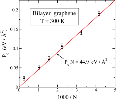
Figure 13: Critical pressure $P_{c}$ as a function of the inverse cell size at $T$ = 300 K. Solid circles represent data derived from MD simulations of bilayer graphene under in-plane stress. The solid line was calculated using Eq. (27).

Calculations based on the SCSA predict a universal behavior for scaling exponents in the thermodynamic limit ($N\to\infty$) Le Doussal and Radzihovsky (1992); Kosmrlj and Nelson (2013); Le Doussal and Radzihovsky (2018). This means that the exponents presented above should coincide for 2D systems (including monolayers and bilayers) in the large-size limit. According to such calculations, universality is approached for system size larger than a crossover scale given by the so-called Ginzburg length, $L_{G}$. This temperature-dependent length can be estimated for graphene (using the bending constant $\kappa$ and Young’s modulus $E_{p}$) to be around $40-50$ Å at $T=300$ K de Andres et al. (2012b); Mauri et al. (2020). This corresponds in our notation to a system size $N_{G}\sim 900$. For bilayer graphene, we have considered here simulation cells with length sides up to 150 Å, well above those values of $L_{G}$. One can, however, understand $L_{G}$ as a reference length for the crossover to a regime where universality is approached, and a direct detection of this universality could be only found for lengths clearly larger than $L_{G}$. In any case, from the results of our simulations for bilayer (with $L$ up to 150 Å) and monolayer graphene presented here, we do not find any evidence or trend indicating that such a kind of universality will appear for results derived from simulations using larger cells. Thus, if such kind of universality is in fact a physical aspect of 2D crystalline membranes, as predicted by the SCSA, it has not yet been observed from atomistic simulations with interaction potentials mimicking those of actual materials, as graphene.

VIII Summary

MD simulations allow us to gain insight into elastic properties of 2D materials, as well as on their stability under external stress. We have presented here the results of extensive simulations of bilayer graphene using a well-checked interatomic potential, for a wide range of temperatures, in-plane stresses, and system sizes. We have concentrated on physical properties such as the excess area, interlayer spacing, interatomic distance, elastic constants, in-plane compression modulus, and atomic MSF in the out-of-plane direction.

The elastic constants are found to appreciably change as a function of temperature, especially $c_{12}$. This causes a reduction of the Poisson’s ratio for rising $T$. The in-plane compression modulus $B_{p}$ has been obtained from the fluctuations of the in-plane area, a procedure which yields results consistent with those derived from the elastic constants of the bilayer.

For bilayer graphene under in-plane stress, we find a divergence of the MSF $(\Delta h)^{2}$ for an in-plane pressure $P_{c}(N)$, which corresponds to the limit of mechanical stability of the material. This divergence is accompanied by a vanishing of the in-plane compression modulus, or a divergence of the compressibility $\xi_{p}=1/B_{p}$.

Finite-size effects are found to be important for several properties of bilayer graphene. The spinodal pressure $P_{c}$ is found to scale with system size as $1/N$. A similar scaling with the inverse size is obtained for the MSF of the interlayer spacing: $(\Delta d)^{2}\sim N^{-1}$. The atomic out-of-plane MSF also follows a power law $(\Delta h)^{2}\sim N^{\alpha}$ with an exponent $\alpha$ = 0.69. For $B_{p}$, we find for $N>500$ at $T=300$ K a dependence $B_{p}\sim N^{-\zeta}$, with an exponent $\zeta=0.086$.

Comparing the simulation results with those obtained from a HA gives insight into finite-temperature anharmonic effects. Thus, for the atomic MSF in the out-of-plane direction, a HA predicts a linear dependence of $(\Delta h)^{2}$ with system size $N$, to be compared with the sublinear dependence obtained from the simulations.

The change with system size $N$ of $(\Delta h)^{2}$ and the modulus $B_{p}$ for bilayer graphene is slower (i.e., less slope in Figs. 11 and 12) than for the monolayer. This is indeed due to interlayer interactions, which manifests themselves in the presence of the layer-breathing ZO’ phonon branch. According to calculations based on the SCSA, the size dependence of physical observables such as $(\Delta h)^{2}$ or the in-plane modulus $B_{p}$ should be controlled, for large $N$, by universal exponents independent of the particular details of the considered 2D system (monolayer or bilayer graphene in our case). We have not observed this universality from our MD simulations for cell size up to 150 Å, and a clarification of this question remains as a challenge for future research.

We finally note that MD simulations as those presented here can give information on the properties of graphene multilayers under stress. This may yield insight into the relative stability of such multilayers in a pressure-temperature phase diagram. Moreover, nuclear quantum effects can affect the mechanical properties of graphene bilayers and multilayers at low temperatures, as shown earlier for graphite. This question can be addressed using atomistic simulations with techniques such as path-integral molecular dynamics.

Appendix A Updates of the LCBOPII model

A.1 Torsion term

The torsion term $t_{ij}$ in the original LCBOPII model Los et al. (2005) was modified to improve the value of the bending rigidity, $\kappa$, in graphene. Eq. (36) in the original paper was changed in the following way:

$$t_{ij}(\tilde{y},\tilde{z})=(1-\tilde{z}^{3})(1+\tilde{z}(1+\tilde{z})\chi(\tilde{y}))\tau_{0}(\tilde{y})+\tilde{z}^{3}\tau_{1}(\tilde{y})\>,$$ (28)

where the variables $\tilde{y},\tilde{z}$ are defined as in Ref. Los et al. (2005). The new functions are:

$$\tau_{0}(\tilde{y})=A_{t1}+A_{t2}\tilde{y}^{2}(3-2\tilde{y}^{2})\>,$$ (29)

$$\tau_{1}(\tilde{y})=\frac{B_{t1}+B_{t2}\tilde{y}^{2}+B_{t3}\tilde{y}^{4}}{1+B_{t4}\tilde{y}^{2}}\>,$$ (30)

$$\chi(\tilde{y})=C_{t1}+C_{t2}\tilde{y}^{2}\>.$$ (31)

Values of the constants are: $A_{t1}=-0.049$, $A_{t2}=-0.022$, $B_{t1}=-0.295$, $B_{t2}=-3.361$, $B_{t3}=1.150$, $B_{t4}=19.616$, $C_{t1}=3.35$, $C_{t2}=-2.6$. Units of energy and length are eV and Å, respectively, as in the original paper.

A.2 Long-range-interaction

The longe-range term $V^{lr}(r)$ of the original LCBOPII model Los et al. (2005) has been modified to improve the value of the interaction energy between both graphene layers in the bilayer. The long-range interaction $V^{lr}(r)$ between two carbon atoms, given in Eq. (42) of the original paper Los et al. (2005), is changed by a new one, but only when the two carbon atoms at a distance $r$ are located at different graphene layers. The modified long-range interaction has the following form:

$$V_{mod}^{lr}(r)=\left(c_{1}e^{-\alpha(r-r_{0})}-\frac{c_{2}}{r^{6}}+c_{3}\frac{e^{-2\alpha(r-r_{0})}}{r^{6}}\right)S_{lr}^{down}(r)$$

$$\text{if}\;r\leq 5.1\;\text{\AA}$$

$$V_{mod}^{lr}(r)=\left[(d_{1}+d_{2}r)(r-6)^{2}\right]S_{lr}^{down}(r)\>,$$

$$\text{if}\;5.1\;\text{\AA}\;<r<6\;\text{\AA}\>,$$

$$V_{mod}^{lr}(r)=0,\hskip 14.22636pt\text{if}\;r\geq 6\;\text{\AA}\>.$$

The function $S_{lr}^{down}(r)$ smoothly cuts off the long-range interactions at 6 Å and it is defined in Tab. I of Ref. Los et al. (2005). Values of the constants are: $r_{0}=3.7157,\>c_{1}=3.0748\times 10^{-3},\>c_{2}=353.1877,\>c_{3}=334.9434,\;\alpha=5.4767\times 10^{-2}\>d_{1}=-4.2249\times 10^{-3},\;\mathrm{and}\;d_{2}=6.1914\times 10^{-4}$. Units of energy and length are eV and Å, respectively, as in the original paper.

Appendix B Excess area

A relation between the in-plane and real areas can be obtained from a continuum description of a graphene sheet, which considers the vibrational modes in the $z$ direction. The instantaneous real area per atom, $S_{r}^{*}$, can be expressed in the continuum limit as Imparato (2006); Waheed and Edholm (2009); Ramírez and Herrero (2017)

$$S_{r}^{*}=\frac{1}{N}\int_{0}^{L_{x}}\int_{0}^{L_{y}}dx\,dy\,\sqrt{1+|\nabla h({\bf r})|^{2}}\;,$$ (32)

where ${\bf r}\equiv(x,y)$ is the 2D position and $h({\bf r})$ indicates the height of the surface, i.e. the distance to the mean $xy$ plane of the sheet. For small $|\nabla h({\bf r})|$, i.e., $(\partial h/\partial x)^{2}+(\partial h/\partial y)^{2}\ll 1$ (which is verified here), one has

$$S_{r}^{*}\approx\frac{1}{N}\int_{0}^{L_{x}}\int_{0}^{L_{y}}dx\,dy\,\left[1+\frac{1}{2}|\nabla h({\bf r})|^{2}\right]\;.$$ (33)

The out-of-plane displacement $h({\bf r})$ can be written as a Fourier series

$$h({\bf r})=\frac{1}{\sqrt{N}}\sum_{\bf k}{\rm e}^{i{\bf k\cdot r}}H({\bf k})\;,$$ (34)

with wavevectors ${\bf k}=(k_{x},k_{y})$ in the 2D hexagonal Brillouin zone, i.e., $k_{x}=2\pi n_{x}/L_{x}$ and $k_{y}=2\pi n_{y}/L_{y}$ with integers $n_{x}$ and $n_{y}$ Ramírez et al. (2016). The Fourier components are given by

$$H({\bf k})=\frac{\sqrt{N}}{L_{x}L_{y}}\int_{0}^{L_{x}}\int_{0}^{L_{y}}dx\,dy\,{\rm e}^{-i{\bf k\cdot r}}h({\bf r})\;.$$ (35)

The thermal average of the atomic MSF in the $z$-direction is given from the Fourier components by

$$\langle h({\bf r})^{2}\rangle=\frac{1}{N}\sum_{\bf k}\langle|H({\bf k})|^{2}\rangle\;.$$ (36)

From Eq. (34), we have

$$\nabla h({\bf r})=\frac{i}{\sqrt{N}}\sum_{\bf k}{\bf k}\,{\rm e}^{i{\bf k\cdot r}}H({\bf k})\;,$$ (37)

and

$$\langle|\nabla h({\bf r})|^{2}\rangle=\frac{1}{N}\sum_{\bf k}k^{2}\langle|H({\bf k})|^{2}\rangle\;,$$ (38)

because $\langle H({\bf k}_{1})H({\bf k}_{2})^{*}\rangle=0$ for ${\bf k}_{1}\neq{\bf k}_{2}$.

Then, using Eqs. (33) and (38), the mean real area per atom can be written as

$$S_{r}=\langle S_{r}^{*}\rangle=S_{p}\left(1+\frac{1}{2N}\sum_{\bf k}k^{2}\langle|H({\bf k})|^{2}\rangle\right)\;,$$ (39)

with $S_{p}=L_{x}L_{y}/N$. For uncoupled vibrational modes in the out-of-plane $z$ direction (i.e., in a HA), $\langle|H({\bf k})|^{2}\rangle$ may be expressed as a sum of MSFs:

$$\langle|H({\bf k})|^{2}\rangle=\sum_{j}\langle|\xi_{j}({\bf k})|^{2}\rangle$$ (40)

with $\langle|\xi_{j}({\bf k})|^{2}\rangle=k_{B}T/m\omega_{j}({\bf k})^{2}$, so that we have for the excess area:

$$\Phi=\frac{S_{r}-S_{p}}{S_{p}}=\frac{k_{B}T}{2mN}\sum_{j,{\bf k}}\frac{k^{2}}{\omega_{j}({\bf k})^{2}}\;.$$ (41)

The sum in $j$ in Eqs. (40) and (41) runs over the phonon bands with atom displacements in the $z$ direction (ZA, ZO’, and the two-fold degenerate ZO branch). We note that the in-plane area fluctuates in our simulations, but its fluctuations are not considered in the harmonic calculation presented here.

Appendix C Spinodal pressure

Close to a spinodal point, the free energy at temperature $T$ can be written as Maris (1991); Boronat et al. (1994); Ramírez and Herrero (2020)

$$F=F_{c}+a_{1}\,(S_{p}-S_{p}^{c})+a_{3}\,(S_{p}-S_{p}^{c})^{3}+...\;,$$ (42)

where $F_{c}$ and $S_{p}^{c}$ are the free energy and in-plane area at the spinodal point. At this point one has $\partial^{2}F/\partial S_{p}^{2}=0$, so that a quadratic term does not appear on the r.h.s of Eq. (42), i.e., $a_{2}=0$. The coefficients $a_{i}$ are in general dependent of the temperature.

The pressure is

$$P=-\frac{\partial F}{\partial S_{p}}=-a_{1}-3a_{3}\,(S_{p}-S_{p}^{c})^{2}+...\;,$$ (43)

and $P_{c}=-a_{1}$ is the spinodal pressure, as it corresponds to the area $S_{p}^{c}$. The 2D modulus of hydrostatic compression is given by

$$B_{p}=\frac{S_{p}}{n}\,\frac{\partial^{2}F}{\partial S_{p}^{2}}=-\frac{S_{p}}{n}\,\frac{\partial P}{\partial S_{p}}\;.$$ (44)

where $n$ is the number of sheets in the 2D material. Then, to leading order in an expansion in powers of $S_{p}-S_{p}^{c}$, we have

$$B_{p}=\frac{6a_{3}}{n}S_{p}^{c}(S_{p}-S_{p}^{c})\;,$$ (45)

or, considering Eq. (43),

$$B_{p}=\frac{2}{n}\sqrt{3a_{3}}\,S_{p}^{c}\,(P_{c}-P)^{1/2}\;.$$ (46)

References

- Hone et al. (2000) J. Hone, B. Batlogg, Z. Benes, A. T. Johnson, and J. E. Fischer, Science 289, 1730 (2000).
- Geim and Novoselov (2007) A. K. Geim and K. S. Novoselov, Nature Mater. 6, 183 (2007).
- Katsnelson (2007) M. I. Katsnelson, Mater. Today 10, 20 (2007).
- Cea and Guinea (2021) T. Cea and F. Guinea, PNAS USA 118, e2107874118 (2021).
- Bhowmik et al. (2022) S. Bhowmik, B. Ghawri, N. Leconte, S. Appalakondaiah, M. Pandey, P. S. Mahapatra, D. Lee, K. Watanabe, T. Taniguchi, J. Jung, et al., Nature Phys. 18, 639 (2022).
- Cao et al. (2018) Y. Cao, V. Fatemi, S. Fang, K. Watanabe, T. Taniguchi, E. Kaxiras, and P. Jarillo-Herrero, Nature 556, 43 (2018).
- Yankowitz et al. (2019) M. Yankowitz, S. Chen, H. Polshyn, Y. Zhang, K. Watanabe, T. Taniguchi, D. Graf, A. F. Young, and C. R. Dean, Science 363, 1059 (2019).
- Gonzalez-Arraga et al. (2017) L. A. Gonzalez-Arraga, J. L. Lado, F. Guinea, and P. San-Jose, Phys. Rev. Lett. 119, 107201 (2017).
- Sboychakov et al. (2018) A. O. Sboychakov, A. V. Rozhkov, A. L. Rakhmanov, and F. Nori, Phys. Rev. Lett. 120, 266402 (2018).
- Cao et al. (2018) Y. Cao, V. Fatemi, A. Demir, S. Fang, S. L. Tomarken, J. Y. Luo, J. D. Sanchez-Yamagishi, K. Watanabe, T. Taniguchi, E. Kaxiras, et al., Nature 556, 80 (2018).
- Meyer et al. (2007) J. C. Meyer, A. K. Geim, M. I. Katsnelson, K. S. Novoselov, D. Obergfell, S. Roth, C. Girit, and A. Zettl, Solid State Commun. 143, 101 (2007).
- Gibertini et al. (2010) M. Gibertini, A. Tomadin, M. Polini, A. Fasolino, and M. I. Katsnelson, Phys. Rev. B 81, 125437 (2010).
- Safran (1994) S. A. Safran, Statistical Thermodynamics of Surfaces, Interfaces, and Membranes (Addison Wesley, New York, 1994).
- Nelson et al. (2004) D. Nelson, T. Piran, and S. Weinberg, Statistical Mechanics of Membranes and Surfaces (World Scientific, London, 2004).
- Chacón et al. (2015) E. Chacón, P. Tarazona, and F. Bresme, J. Chem. Phys. 143, 034706 (2015).
- Ruiz-Herrero et al. (2012) T. Ruiz-Herrero, E. Velasco, and M. F. Hagan, J. Phys. Chem. B 116, 9595 (2012).
- Amorim et al. (2014) B. Amorim, R. Roldan, E. Cappelluti, A. Fasolino, F. Guinea, and M. I. Katsnelson, Phys. Rev. B 89, 224307 (2014).
- Ramírez and Herrero (2018a) R. Ramírez and C. P. Herrero, J. Chem. Phys. 149, 041102 (2018a).
- Zakharchenko et al. (2010) K. V. Zakharchenko, J. H. Los, M. I. Katsnelson, and A. Fasolino, Phys. Rev. B 81, 235439 (2010).
- Herrero and Ramírez (2019) C. P. Herrero and R. Ramírez, J. Chem. Phys. 150, 204707 (2019).
- Balandin (2011) A. A. Balandin, Nature Mater. 10, 569 (2011).
- Herrero and Ramírez (2020) C. P. Herrero and R. Ramírez, Phys. Rev. B 101, 035405 (2020).
- Michel and Verberck (2008) K. H. Michel and B. Verberck, Phys. Rev. B 78, 085424 (2008).
- Savini et al. (2011) G. Savini, Y. J. Dappe, S. Oberg, J.-C. Charlier, M. I. Katsnelson, and A. Fasolino, Carbon 49, 62 (2011).
- de Andres et al. (2012a) P. L. de Andres, F. Guinea, and M. I. Katsnelson, Phys. Rev. B 86, 245409 (2012a).
- Los et al. (2016) J. H. Los, A. Fasolino, and M. I. Katsnelson, Phys. Rev. Lett. 116, 015901 (2016).
- Lee et al. (2008) C. Lee, X. Wei, J. W. Kysar, and J. Hone, Science 321, 385 (2008).
- Polyzos et al. (2015) I. Polyzos, M. Bianchi, L. Rizzi, E. N. Koukaras, J. Parthenios, K. Papagelis, R. Sordan, and C. Galiotis, Nanoscale 7, 13033 (2015).
- Androulidakis et al. (2015) C. Androulidakis, E. N. Koukaras, J. Parthenios, G. Kalosakas, K. Papagelis, and C. Galiotis, Sci. Reports 5, 18219 (2015).
- Papageorgiou et al. (2017) D. G. Papageorgiou, I. A. Kinloch, and R. J. Young, Progr. Mater. Sci. 90, 75 (2017).
- Nicholl et al. (2017) R. J. T. Nicholl, N. V. Lavrik, I. Vlassiouk, B. R. Srijanto, and K. I. Bolotin, Phys. Rev. Lett. 118, 266101 (2017).
- Gao et al. (2018) Y. Gao, T. Cao, F. Cellini, C. Berger, W. A. de Heer, E. Tosatti, E. Riedo, and A. Bongiorno, Nature Nano. 13, 133 (2018).
- Liu and Peng (2018) A. Liu and Q. Peng, Micromachines 9, 440 (2018).
- Ovchinnikov et al. (2018) O. S. Ovchinnikov, A. O’Hara, R. J. T. Nicholl, J. A. Hachtel, K. Bolotin, A. Lupini, S. Jesse, A. P. Baddorf, S. V. Kalinin, A. Y. Borisevich, et al., 2D Mater. 5, 041008 (2018).
- Chen et al. (2021) J. Chen, J. Pei, and H. Zhao, J. Phys. Chem. C 125, 19345 (2021).
- Monji et al. (2022) F. Monji, D. Desai, and C. Jian, J. Mater. Sci. 57, 2514 (2022).
- Cao et al. (2018) Q. Cao, X. Geng, H. Wang, P. Wang, A. Liu, Y. Lan, and Q. Peng, Crystals 8, 357 (2018).
- Amorim et al. (2016) B. Amorim, A. Cortijo, F. de Juan, A. G. Grushine, F. Guinea, A. Gutierrez-Rubio, H. Ochoa, V. Parente, R. Roldan, P. San-Jose, et al., Phys. Rep. 617, 1 (2016).
- Fasolino et al. (2007) A. Fasolino, J. H. Los, and M. I. Katsnelson, Nature Mater. 6, 858 (2007).
- Akatyeva and Dumitrica (2012) E. Akatyeva and T. Dumitrica, J. Chem. Phys. 137, 234702 (2012).
- Magnin et al. (2014) Y. Magnin, G. D. Foerster, F. Rabilloud, F. Calvo, A. Zappelli, and C. Bichara, J. Phys.: Condens. Matter 26, 185401 (2014).
- Koukaras et al. (2016) E. N. Koukaras, C. Androulidakis, G. Anagnostopoulos, K. Papagelis, and C. Galiotis, Extreme Mech. Lett. 8, 191 (2016).
- Zheng et al. (2019) S. Zheng, Q. Cao, S. Liu, and Q. Peng, J. Composites Sci. 3, 2 (2019).
- Los et al. (2005) J. H. Los, L. M. Ghiringhelli, E. J. Meijer, and A. Fasolino, Phys. Rev. B 72, 214102 (2005).
- Ghiringhelli et al. (2005) L. M. Ghiringhelli, J. H. Los, A. Fasolino, and E. J. Meijer, Phys. Rev. B 72, 214103 (2005).
- Ramírez et al. (2016) R. Ramírez, E. Chacón, and C. P. Herrero, Phys. Rev. B 93, 235419 (2016).
- Zakharchenko et al. (2009) K. V. Zakharchenko, M. I. Katsnelson, and A. Fasolino, Phys. Rev. Lett. 102, 046808 (2009).
- Ramírez and Herrero (2017) R. Ramírez and C. P. Herrero, Phys. Rev. B 95, 045423 (2017).
- Herrero and Ramírez (2016) C. P. Herrero and R. Ramírez, J. Chem. Phys. 145, 224701 (2016).
- Lambin (2014) P. Lambin, Appl. Sci. 4, 282 (2014).
- Tuckerman and Hughes (1998) M. E. Tuckerman and A. Hughes, in Classical and Quantum Dynamics in Condensed Phase Simulations, edited by B. J. Berne, G. Ciccotti, and D. F. Coker (Word Scientific, Singapore, 1998), p. 311.
- Allen and Tildesley (1987) M. P. Allen and D. J. Tildesley, Computer simulation of liquids (Clarendon Press, Oxford, 1987).
- Martyna et al. (1996) G. J. Martyna, M. E. Tuckerman, D. J. Tobias, and M. L. Klein, Mol. Phys. 87, 1117 (1996).
- Behroozi (1996) F. Behroozi, Langmuir 12, 2289 (1996).
- Sfyris et al. (2015) D. Sfyris, E. N. Koukaras, N. Pugno, and C. Galiotis, J. Appl. Phys. 118, 075301 (2015).
- Memarian et al. (2015) F. Memarian, A. Fereidoon, and M. D. Ganji, Superlattices Microstruct. 85, 348 (2015).
- Zou et al. (2016) J.-H. Zou, Z.-Q. Ye, and B.-Y. Cao, J. Chem. Phys. 145, 134705 (2016).
- Anastasi et al. (2016) A. A. Anastasi, K. Ritos, G. Cassar, and M. K. Borg, Mol. Simul. 42, 1502 (2016).
- Ghasemi and Rajabpour (2017) H. Ghasemi and A. Rajabpour, J. Phys. Conf. Series 785, 012006 (2017).
- Yan et al. (2008) J.-A. Yan, W. Y. Ruan, and M. Y. Chou, Phys. Rev. B 77, 125401 (2008).
- Karssemeijer and Fasolino (2011) L. J. Karssemeijer and A. Fasolino, Surf. Sci. 605, 1611 (2011).
- Koukaras et al. (2015) E. N. Koukaras, G. Kalosakas, C. Galiotis, and K. Papagelis, Sci. Rep. 5, 12923 (2015).
- Singh and Hennig (2013) A. K. Singh and R. G. Hennig, Phys. Rev. B 87, 094112 (2013).
- Wirtz and Rubio (2004) L. Wirtz and A. Rubio, Solid State Commun. 131, 141 (2004).
- Amorim and Guinea (2013) B. Amorim and F. Guinea, Phys. Rev. B 88, 115418 (2013).
- Ramírez and Herrero (2019) R. Ramírez and C. P. Herrero, J. Chem. Phys. 151, 224107 (2019).
- Herrero and Ramírez (2021) C. P. Herrero and R. Ramírez, Phys. Rev. B 104, 054113 (2021).
- Lin et al. (2018) M.-L. Lin, J.-B. Wu, X.-L. Liu, and P.-H. Tan, J. Raman Spectr. 49, 19 (2018).
- Newnham (2005) R. E. Newnham, Properties of Materials. Anisotropy, Symmetry, Structure. (Oxford University Press, Oxford, 2005).
- Blakslee et al. (1970) O. L. Blakslee, D. G. Proctor, E. J. Seldin, G. B. Spence, and T. Weng, J. Appl. Phys. 41, 3373 (1970).
- Nicklow et al. (1972) R. Nicklow, N. Wakabayashi, and H. G. Smith, Phys. Rev. B 5, 4951 (1972).
- Gao and Huang (2014) W. Gao and R. Huang, J. Mech. Phys. Solids 66, 42 (2014).
- Imparato (2006) A. Imparato, J. Chem. Phys. 124, 154714 (2006).
- Waheed and Edholm (2009) Q. Waheed and O. Edholm, Biophys. J. 97, 2754 (2009).
- Nicholl et al. (2015) R. J. T. Nicholl, H. J. Conley, N. V. Lavrik, I. Vlassiouk, Y. S. Puzyrev, V. P. Sreenivas, S. T. Pantelides, and K. I. Bolotin, Nature Commun. 6, 8789 (2015).
- Helfrich and Servuss (1984) W. Helfrich and R. M. Servuss, Nuovo Cimento D 3, 137 (1984).
- Fournier and Barbetta (2008) J.-B. Fournier and C. Barbetta, Phys. Rev. Lett. 100, 078103 (2008).
- Herrero and Ramírez (2018a) C. P. Herrero and R. Ramírez, J. Chem. Phys. 148, 102302 (2018a).
- Ashcroft and Mermin (1976) N. W. Ashcroft and N. D. Mermin, Solid State Physics (Saunders College, Philadelphia, 1976).
- Marsden et al. (2018) B. Marsden, A. Mummery, and P. Mummery, Proc. Royal Soc. A 474, 20180075 (2018).
- Herrero and Ramírez (2017) C. P. Herrero and R. Ramírez, Phys. Chem. Chem. Phys. 19, 31898 (2017).
- Le Doussal and Radzihovsky (1992) P. Le Doussal and L. Radzihovsky, Phys. Rev. Lett. 69, 1209 (1992).
- Kosmrlj and Nelson (2013) A. Kosmrlj and D. R. Nelson, Phys. Rev. E 88, 012136 (2013).
- Le Doussal and Radzihovsky (2018) P. Le Doussal and L. Radzihovsky, Annals Phys. 392, 340 (2018).
- Burmistrov et al. (2018) I. S. Burmistrov, I. V. Gornyi, V. Y. Kachorovskii, M. I. Katsnelson, J. H. Los, and A. D. Mirlin, Phys. Rev. B 97, 125402 (2018).
- Landau and Lifshitz (1980) L. D. Landau and E. M. Lifshitz, Statistical Physics (Pergamon, Oxford, 1980), 3rd ed.
- Herrero and Ramírez (2018b) C. P. Herrero and R. Ramírez, Phys. Rev. B 97, 195433 (2018b).
- Sciortino et al. (1995) F. Sciortino, U. Essmann, H. E. Stanley, M. Hemmati, J. Shao, G. H. Wolf, and C. A. Angell, Phys. Rev. E 52, 6484 (1995).
- Herrero (2003) C. P. Herrero, Phys. Rev. B 68, 172104 (2003).
- Callen (1985) H. B. Callen, Thermodynamics and an Introduction to Thermostatistics (John Wiley, New York, 1985).
- Speedy (1982) R. J. Speedy, J. Phys. Chem. 86, 3002 (1982).
- Ramírez and Herrero (2020) R. Ramírez and C. P. Herrero, Phys. Rev. B 101, 235436 (2020).
- Ramírez and Herrero (2018b) R. Ramírez and C. P. Herrero, Phys. Rev. B 97, 235426 (2018b).
- Tröster (2013) A. Tröster, Phys. Rev. B 87, 104112 (2013).
- de Andres et al. (2012b) P. L. de Andres, F. Guinea, and M. I. Katsnelson, Phys. Rev. B 86, 144103 (2012b).
- Mauri et al. (2020) A. Mauri, D. Soriano, and I. M. Katsnelson, Phys. Rev. B 102, 165421 (2020).
- Maris (1991) H. J. Maris, Phys. Rev. Lett. 66, 45 (1991).
- Boronat et al. (1994) J. Boronat, J. Casulleras, and J. Navarro, Phys. Rev. B 50, 3427 (1994).