Quantum Vector Signal Analyzer

Abstract

A technique that allows a harmonic oscillator to be used as a wideband, vector signal analyzer is described and demonstrated using a single trapped ⁴⁰Ca⁺ ion cooled near its motional ground state. Further, the analyzer is shown to be compatible with both quantum amplification via squeezing and measurement in the Fock basis, allowing performance beyond the standard quantum limit. In addition to providing an attractive platform for quantum sensing of small fields, the technique allows in situ calibration of qubit control lines in systems using quantum harmonic oscillators and transduction of external, non-resonant drives into oscillator motion. This technique is extendable to other quantum harmonic oscillator systems.

Harmonic oscillators controlled at the single quanta level provide quantum-limited metrology capabilities. For single quantum harmonic oscillators (QHOs), it has been shown that non-classical Fock states provide optimal precision and sensitivity for measurements of displacements with unknown phase, and they have been used to measure the amplitude and frequency of an oscillator below the standard quantum limit (SQL) [1, 2]. Further, using squeezing to provide ‘quantum amplification’ the sensitivity of a QHO to a resonant force has been enhanced by roughly an order of magnitude [3] and entanglement of the collective spin states of trapped ions with a shared motional mode has provided sensitivity to amplitudes 40$\times$ below the zero-point fluctuations of the oscillator [4], as well as sensitivity to DC displacements roughly 9 dB below the SQL [5].

However, despite important work using motional cat states [6] or amplitude modulated displacement of Fock states [7] to measure the noise spectrum of an oscillator, QHO-based field sensing has been limited to frequencies from DC up to the natural frequency of the oscillator. Further, measuring the phase of the applied field remains challenging since measurement is typically performed in the Fock basis. Here, we show that by parametrically driving a QHO with an amplitude modulated field, a QHO can be used to sense the amplitude, frequency, and phase of an unknown field. This effect can be understood as a heterodyne detection that results from the phase sensitive interference of multiple, three-phonon Raman transitions to generate a displacement of the oscillator. In what follows, we describe the interaction responsible for and the operation of a quantum vector signal analyzer (QVSA) based on a single trapped ion. We benchmark our method by measuring the known transfer function of a commercial filter and demonstrate in situ direct calibration of a qubit control line from 20 MHz to 300 MHz, limited by our direct digital synthesis (DDS) capabilities. We characterize the sensitivity and precision of the QVSA at a frequency near the middle of this range (82 MHz) and find an amplitude sensitivity (without the use of an pre-amplifier) of 51(10) $\mu$V/$\sqrt{\textup{Hz}}$ with minimal detectable voltage 3.8(8)$\mu$V; a frequency sensitivity of 28(5) Hz/$\sqrt{\textup{Hz}}$ with minimum resolution 2$\pi\cdot 3.1(5)$ Hz; and a phase sensitivity of 49(11) mrad/$\sqrt{\textup{Hz}}$ with minimum phase resolution $3.0(7)$ mrad. We further show that the technique is compatible with quantum amplification [3, 8, 9, 10] and use a squeezing operation to realize a 9.0(4) dB gain in voltage sensitivity and demonstrate an amplitude sensitivity 1.7(1.0) dB below the SQL. We also show evidence that with a strong parametric drive the resulting interaction intrinsically squeezes the QHO, allowing the realization of quantum amplification without an external squeeze operator. Finally, we discuss straightforward improvements of the technique that should improve the quoted sensitivities by several orders of magnitude.

To demonstrate this technique, we use a QHO realized via a motional mode at $\omega\approx 2\pi\cdot 1$ MHz of a single ⁴⁰Ca⁺ ion held in a cryogenically cooled (4.5 K) linear Paul trap. The QHO is initialized and readout via coupling through a Jaynes-Cummings Hamiltonian to an optical qubit defined on the $\{\ket{{}^{2}D_{\frac{5}{2}},m_{J}=-\frac{5}{2}},\ket{{}^{2}S_{\frac{1}{2}},m_{J}=-\frac{1}{2}}\}$ electronic states of ⁴⁰Ca⁺. Doppler cooling of the ⁴⁰Ca⁺ followed by resolved sideband cooling on the narrow optical qubit transition [11] prepares the motional ground state with a measured average phonon number of $\langle n\rangle=0.03(2)$ (see SI).

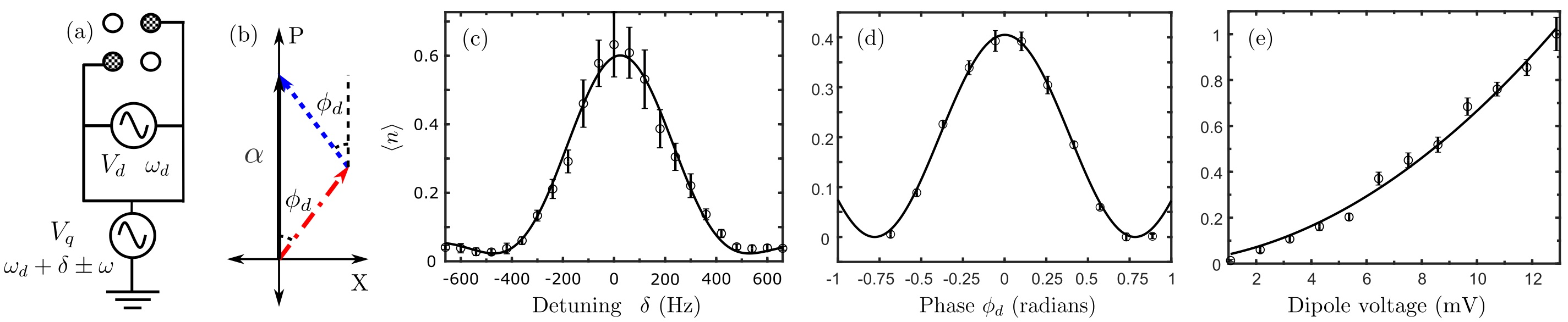
Figure 1: Implementation of the quantum vector signal analyzer (QVSA). (a) Schematic of the coupling of the QVSA drive to the quadrupole ion trap. Two quadruple fields are coupled onto electrodes to diagnose dipole signal ($V_{d}$). (b) The phase space diagram shows that the phase sensitivity of QVSA results from phase dependent displacement $\alpha$ caused by interference between multiple three-phonon Raman transitions; Each transition is initiated by one quadrupole and one dipole field. (c) ($V_{d}\approx 29.24$ mV, $V_{q}\approx 2.924$ V) The lineshape $\langle n\rangle=|\alpha|^{2}$ versus detuning $\delta$. Here, the quadrupole fields are swept simultaneously across $\omega_{d}$. (d) ($V_{d}\approx 162.2$ mV, $V_{q}\approx 432.6$ mV) The dependence of $\langle n\rangle$ on $\phi_{d}$. Assume the initial phase of quadrupole tones are zero. (e) ($V_{d}\approx 162.2$ mV, $V_{q}\approx 214.6$ mV) The dependence of $\langle n\rangle$ on $V_{q}$. The combination of methods shown in (c)-(e), which were all taken using ($t=1$ ms, $\omega_{d}=2\pi\cdot 82$ MHz, $\omega\approx 2\pi\cdot 0.769$ MHz), provide the means for vector signal analysis. Solid lines are fit using eq.2. Error bars represent one standard error.

To understand the operation of the QVSA, suppose an unknown oscillatory signal with voltage $V_{d}$ at frequency $\omega_{d}$ and phase $\phi_{d}$ is applied to the trap in a dipole configuration (the dipole tone) while two voltages at $V_{q}$ with frequencies at $\omega_{d}+\delta\pm\omega$ are applied to the trap in a quadrupole configuration (the quadrupole tones), as shown in Fig. 1(a). We assume $\omega_{d}\gg\omega\gg\delta$ and the initial phase of quadrupole tones are zero (See SI for more phase relation discussion). The motion of the ion is described by the Hamiltonian:

$$\hat{H}=\omega\hat{a}^{\dagger}\hat{a} +\Omega_{q}\left(\hat{a}+\hat{a}^{\dagger}\right)^{2}\cos{\left(\left(\omega_{d}+\delta\right)t\right)}\cos{\left(\omega t\right)}$$

$$+\Omega_{d}\left(\hat{a}+\hat{a}^{\dagger}\right)\cos{\left(\omega_{d}t+\phi_{d}\right)}.$$ (1)

where $\Omega_{q}=eV_{q}x_{o}^{2}/(\hbar r_{o}^{2})$, $\Omega_{d}=\kappa eV_{d}x_{o}/(\hbar r_{o})$, $r_{o}$ is the trap field radius, $x_{o}=\sqrt{\hbar/(2m\omega)}$ is the zero-point wavefunction of the QHO, and $\kappa$ is a geometrical factor that depends on the motional mode.

The resulting evolution can be understood by noticing that the dipole tone off-resonantly drives $\Delta n=\pm 1$ transitions, while the quadrupole tones off-resonantly drive $\Delta n=\pm 2$. For $\delta<\Omega_{q}\Omega_{d}/(\omega_{d}-2\omega)$, the dipole tone with either quadrupole tone can drive three-phonon Raman transition resulting in a total $\Delta n=\pm 1$. Thus, it is not surprising (see SI) that to second order in the Magnus expansion, the time evolution is approximately given in the interaction picture with respect to the harmonic oscillator by a displacement operator with displacement (see SI):

$$\alpha=\imath\Omega_{q}\Omega_{d}\frac{\omega}{\omega_{d}^{2}-\omega^{2}}\frac{\sin{(\delta t-\phi_{d})+\sin\phi_{d}}}{\delta}.$$ (2)

As a result, the magnitude of the displacement $|\alpha|$ under this interaction depends on the amplitude $V_{d}$, frequency $\omega_{d}$, quadrupole probing field application time $t$, and phase $\phi_{d}$ of the unknown dipole field.

While dependence on $V_{d}$ and $\omega_{d}$ are expected, the dependence of $|\alpha|$ on $\phi_{d}$ is surprising. Typically, when driving a harmonic oscillator the phase of the drive dictates whether the displacement is in position or momentum, not the magnitude of the displacement – this is why it is difficult to perform a phase sensitive measurement in many QHO systems which typically measure in the Fock basis. Here, the sensitivity to phase can be understood as the result of interference between displacement due to the dipole and blue quadrupole tone with displacement from the dipole and red quadrupole (Fig. 1(b)).

Using this dependence we demonstrate vector signal analysis of an ‘unknown’ dipole field $(V_{d},\omega_{d},\phi_{d})$ as follows. First, the QHO is prepared in the ground state $\ket{0}$. Next, the quadrupole tones are applied at a chosen amplitude $\Omega_{q}$ and detuning $\delta$ for a time $t$, creating a coherent state $\ket{\alpha}$. Finally, the average phonon number, $\langle n\rangle=|\alpha|^{2}$, of the QHO is measured from the relative intensity of the red and blue motional sidebands of the optical qubit transition (see SI). This process is scanned across detunings to maximize the displacement, yielding the ‘unknown’ frequency $\omega_{d}$ (Fig. 1(c)). Once $\omega_{d}$ is determined, $\phi_{d}$ is found by repeating the above protocol at $\delta=0$ while varying the phase of the applied quadrupole fields. As shown in Fig. 1(d), the displacement is maximized when the $\phi_{d}$ is zero. With $\omega_{d}$ and $\phi_{d}$ determined, the measurement of $\langle n\rangle$ can be used to determine $V_{d}$. This measurement is shown in Fig. 1(e) for varying the strength of the dipole field, while keeping the quadrupole voltage constant.

Figure 2: Transfer function of a commercial low pass filter. (a-b) $\circ$ and $\diamond$ are measured through QVSA. Solid lines are measured via a commercial vector network analyzer. Each point is composed of $N\approx 13500$ experiments. Error bars represent one standard error. No re-scaling or offset is applied to the data.

To benchmark the system and showcase its use as a vector network analyzer, we measure the transfer function of a commercial low pass filter (Mini-Circuits: SLP-100+). For this measurement, $V_{d}$ and $\phi_{d}$ are measured as a function of frequency with and without the filter inserted. The data is shown in Fig. 2 alongside the measurement from a standard network analyzer (Agilent 8714ES).

As this technique reports the field seen by the QHO, it naturally provides a method for in situ calibration of the filter function of a qubit control line if the qubit is coupled to a QHO. The present system has been designed to demonstrate electric-field gradient gates on molecular ion qubits [12] and we have therefore used this technique to measure the coupling efficiency of qubit control signals from our DDSs to the ion. The measured coupling efficiency is compared against that from a traditional measurement using a pickup antenna and a vector network analyzer over the frequency range accessible with our DDS (20 MHz - 300 MHz) (see SI).

With these demonstrations complete, it is natural to explore the precision and sensitivity limits of the technique. To determine the frequency accuracy, a rough spectrum, like that shown in Fig. 1(c), is first taken to determine the lineshape. Then to maintain a balance between the sensitivity and intrinsic noise in subsequent experiments, measurements of the phonon number are repeatedly taken at the two points in frequency near the half-width, half-maxima to determine the center frequency. The resulting Allan deviation is shown in Fig. 3(a) alongside the SQL $\Delta\delta=2\pi\cdot 0.209/(t\langle\alpha\rangle\sqrt{N})$, where $t=2$ ms is the duration of the QVSA interaction and $N$ is the number of measurements (see SI). The Allan deviation follows the SQL with frequency sensitivity 28(5) Hz/$\sqrt{\textup{Hz}}$ until $N\approx 5000$, and the minimum resolution is 2$\pi\cdot 3.1(5)$ Hz, corresponding to a fractional frequency resolution of $3.8(6)\times 10^{-8}$. The deviation from the SQL is due to changes in the secular frequency $\omega$, which depends on the stability of the temperature and humidity of lab and can drift by $\approx 2\pi\cdot(200-600)$ Hz over the course of these measurements. Similarly, the precision of the phase measurement is determined by a two-point phase measurement at $45\degree$ and $135\degree$ with on-resonant detuning. The Allan deviation of the resulting data is shown in Fig. 3(b) alongside the SQL $\Delta\phi_{d}=1/(2\langle\alpha\rangle\sqrt{2N})$ (see SI). The minimal phase resolution reaches $\approx 3.0(7)$ mrad after $N=11000$ measurements due to the long-term drift of secular frequency mentioned above.

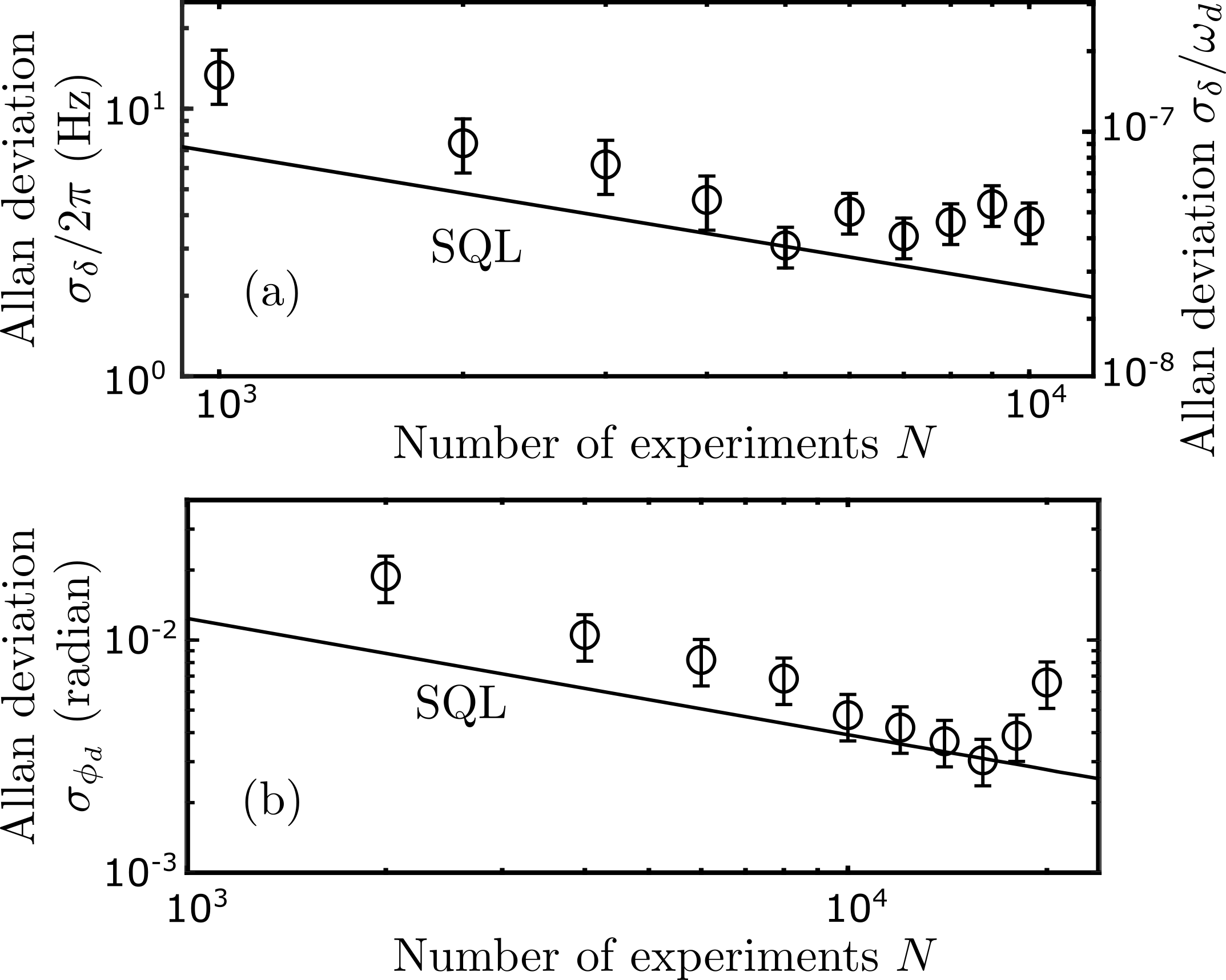
Figure 3: Allan deviation of frequency and phase of a 82 MHz dipole tone. (a) The measured frequency sensitivity is 28(5) Hz/$\sqrt{\textup{Hz}}$ and the minimum resolution is 2$\pi\cdot 3.1(5)$ Hz after 5000 experiments (b) The measured phase sensitivity is 49(11) mrad/$\sqrt{\textup{Hz}}$ and the minimum resolution is $3.0(7)$ mrad after 16000 experiments. Here, the probe time is 2 ms and each experiment takes $\sim$17 ms. The solid lines show the corresponding standard quantum limit (SQL). Experimental sensitivity is limited by drift of the trap secular frequency. Error bars represent one standard error.

To determine the sensitivity of the voltage measurement, a large $V_{q}$ is applied to the electrodes to increase the sensitivity to $V_{d}$ and the resulting phonon number measured. The process is repeated until the noise floor is reached (typically $N\sim 10^{4}$). Fig. 4 (a) shows the minimal detectable voltage ($\Delta$V_min) as a function of drive time at 82 MHz, here $V_{d}=8.4(1)$ V, which is limited by the intrinsic squeezing Hamiltonian term ignored in Eqn. (Quantum Vector Signal Analyzer) . The data roughly follows the SQL until $\approx 1$ ms, where secular frequency instability becomes significant. The measured sensitivity to $V_{d}$ is 51(10) $\mu$V/$\sqrt{\textup{Hz}}$ with a minimum detectable voltage of 3.8(8) $\mu V$ at $N=11000$.

Since the QVSA functions by sensing the displacement of the QHO, it is possible to further increase its voltage sensitivity using the technique of quantum amplification [3, 5]. Adapting quantum amplification to the QVSA requires generating a state, $\hat{S}(r)\ket{0}$, prior to applying the QVSA tones, via e.g. modulation of the trapping potential. Assuming $r\in\mathbb{R}$, this reduces the spread of the QHO wavefunction in position by $e^{-r}$, while increasing the uncertainty in momentum by $e^{r}$ [14, 3]. Next, the system evolves under the QVSA Hamiltonian to produce a displaced squeeze state $\hat{D}(\alpha)\hat{S}(r)\ket{0}$, where for simplicity we assume $\alpha\in\mathbb{R}$. After this evolution, the system is subject to an anti-squeeze operation to produce the state $\hat{S}^{\dagger}(r)\hat{D}(\alpha)\hat{S}(r)\ket{0}$, which has two effects. First, the anti-squeeze operator returns the displaced squeeze state to a coherent state, allowing measurement of the total displacement at the SQL. Second, the anti-squeeze operator amplifies the displacement in position by $e^{r}$. Thus, the resulting coherent state has an amplitude of $e^{r}\alpha$ instead of $\alpha$, allowing sensing of $V_{d}$ below the SQL.

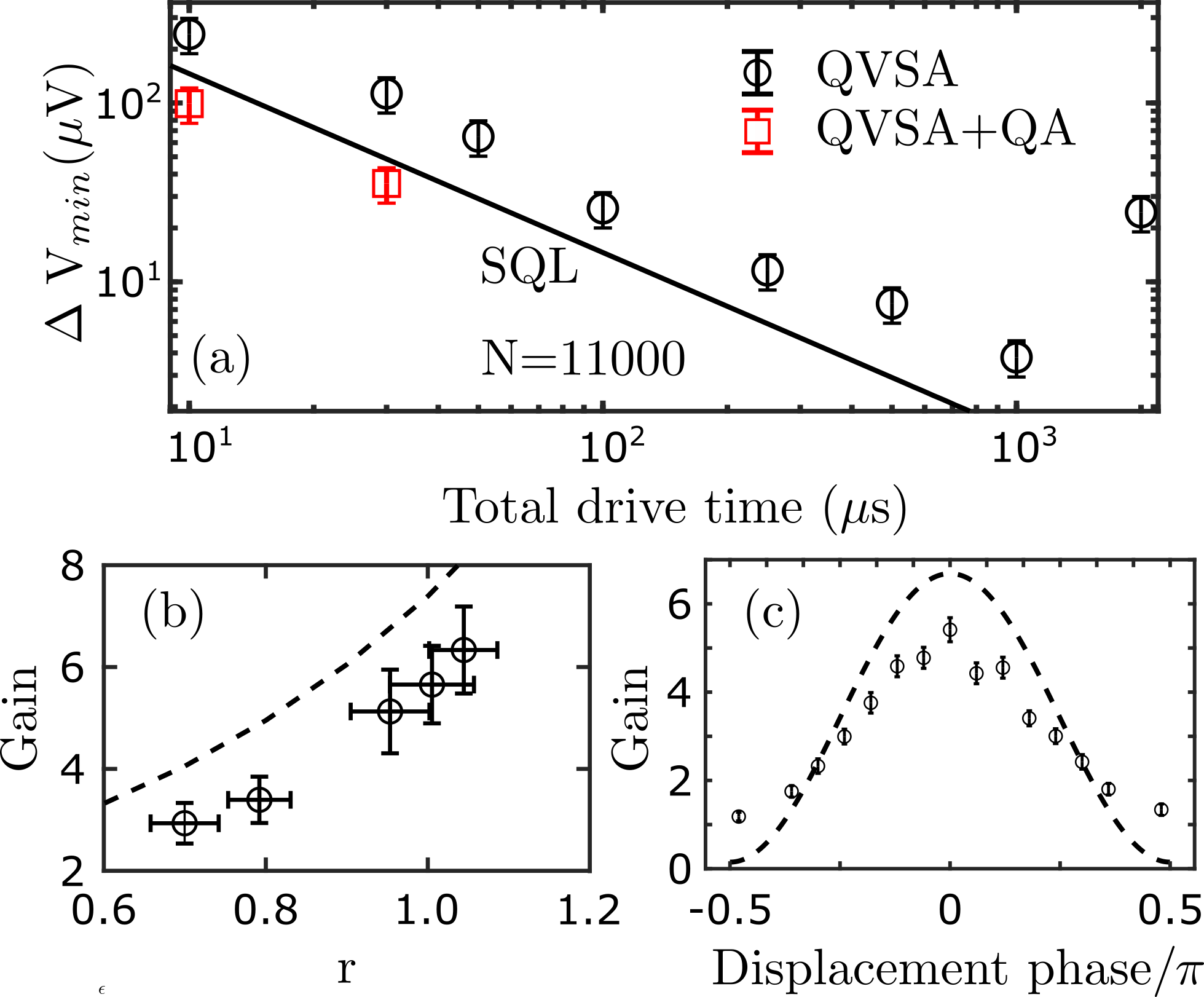
Figure 4: (a) Minimum detectable voltage ($\Delta$V_min) on electrodes with and without quantum amplification (QA). Each data point represents 11,000 experiment, which each require $\sim$17ms. The measured sensitivity to voltage coupled to electrodes is 51(10) $\mu$V/$\sqrt{\textup{Hz}}$ with a minimum detectable voltage of 3.8(8) $\mu$V. Notably, with QA the voltage sensitivity is 1.7 (1.0) dB and 1.4(1.0) dB below the SQL for 10 $\mu$s and 30 $\mu$s, respectively. Error bars represent one standard error. (b-c) Quantum amplification through squeezing. By applying a squeeze operation $\hat{S}(r)$ before and an anti-squeeze operator $\hat{S}^{\dagger}(r)$ after 10 $\mu$s of QVSA operation, an amplification of the final phonon number is observed. The gain depends on the strength $r$ of the squeezer operation (b) and its phase relative to the QVSA displacement (c). The dashed lines represent the maximum achievable gain.

To demonstrate this amplification, we squeeze the oscillator by a parametric trap drive with a maximal coupling strength 2$\pi\cdot 5.5(2)$ kHz. The anti-squeeze operation is realized by the same drive with the phase changed by $\pi$. To verify the fidelity of the anti-squeeze operation, we find that if anti-squeezing is performed directly after the squeeze operation, the phonon number returns to $\langle n\rangle=0.03(2)$, which is indistinguishable from the initial state. Fig. 4(b)) shows the gain in average phonon at the end of the sequence using quantum amplification as a function of $r$. As described above, the maximum amplification occurs when the direction of the displacement in phase space is along the original squeeze direction. Thus, it is important to match the phase between the QVSA displacement operation and the squeezing operation. The relative phase between the QVSA displacement operator and squeeze operator can be varied without affecting the phase difference with the dipole field by simultaneously varying the phase of blue and red quadrupole fields by same amount but with opposite sign, as shown in Fig. 4(c) (see SI) or by changing the phase of the parametric drive. As can be seen in Fig. 4(b-c) a maximum phonon gain of 6.3(9) is achieved. The discrepancy between the realized gain and predicted gain appears to be a result of phase instability between the squeezing and displacement operations. We characterize the voltage sensitivity in the manner previously described and find that the sensitivity is 1.7 (1.0) dB and 1.4(1.0) dB below the SQL for QVSA drive times of 10 $\mu$s and 30 $\mu$s, respectively (see Fig. 4 (a)).

There are several potential modifications that would improve the sensitivity of the QVSA. First, the use of other non-classical motional states, such as cat states [15] or higher-lying Fock states [1] should allow the SQL for the frequency, phase, and amplitude measurements to be surpassed. Second, for implementations based on trapped ions, the voltage sensitivity scales as $m^{-3/2}$, so the use of ions with lighter mass would improve the sensitivity, as well as reduce the time required for ground state cooling (currently 76% of the measurement time is devoted to cooling). Also, improving the secular frequency stability and reducing $r_{o}$ would increase the sensitivity. Third, for use as a vector signal analyzer the signal to be sensed can be passed through a low-noise preamplifier before application to the trap electrodes. With these modification, it appears that for a single trapped Be⁺ ion in the trap of Ref. [2] with a secular frequency stability of $\sim 10$ Hz prepared in the $n=1$ Fock state and with the use of an amplifier, the technique should have a frequency sensitivity of $\approx 0.1$ Hz/$\sqrt{\textrm{Hz}}$, a phase sensitivity of $\approx 0.25$ mrad/$\sqrt{\textrm{Hz}}$, and an amplitude sensitivity of $\approx 86$ fV/$\sqrt{\textrm{Hz}}$.

Another route for increasing the sensitivity is to further increase $V_{q}$. As $V_{q}$ is increased the quadrupole drive they provide also modifies the trapping potential and leads to a phase squeezed state (also called intrinsic squeezing) by the QVSA Hamiltonian (see SI). Thus, with proper anti-squeezing operation following QVSA Hamiltonian, displacement amplified coherent state can be recovered; this will be the subject of future work (see SI).

In summary, we have demonstrated a QVSA capable of providing high sensitivity measurements of amplitude, frequency, and phase of an unknown field with frequency up to a few GHz, using a single trapped ⁴⁰Ca⁺ ion. Unlike existing techniques, which utilize spin-dependent forces, this interaction is entirely motional and thus immune to spin decoherence processes, e.g. magnetic field fluctuations. Further, this scheme is largely implementation-agnostic and thus easily extendable to most QHO architectures. increasing phonon through sideband technique instead of doing the photon correlation. Since this method enables vector analysis of a field applied directly to the QHO, it can be used for an in situ calibration of qubit control lines that feature QHOs. Such calibrations are notoriously challenging since traditional measurement techniques are necessarily ex situ and require changes to measurement conditions, e.g. through stray capacitances of measurement lines, while many in situ techniques are insufficiently general or indirect [6, 16]. The technique may also find use for frequency transduction, for example converting microwave photons into motional phonons in trapped ion systems, or for sensing of electric field noise as a function of frequency. Finally, it is interesting to consider adapting the technique to other platforms. For example, the higher motional frequencies of trapped electrons may allow sensing of THz signals and the use of superconducting resonators with cryogenic amplifiers may allow sensing below the current state of the art.

I Acknowledgement

We thank S. C. Burd, P. Hamilton, and W. Campbell for helpful discussion. This work was supported by NSF (PHY-2110421 and OMA-2016245), AFOSR (130427-5114546), and ARO (W911NF-19-1-0297).

.1 Appendix A: Quadrupole Drive Calculation

Suppose an unknown, oscillatory signal at frequency $\omega_{d}$ is applied to the trap in a dipole configuration while two signals at frequencies at $\omega_{d}+\delta\pm\omega$ are applied to the trap in a quadrupole configuration, as shown in Fig.1(a) of the main text. We assume $\omega_{d}\gg\omega\gg\delta$. The motion of the ion can described by the Hamiltonian

$$\hat{H}/\hbar=\omega\hat{a}^{\dagger}\hat{a}+\Omega_{q}(\hat{a}+\hat{a}^{\dagger})^{2}\cos{\left(\left(\omega_{d}+\delta\right)t\right)}\cos{\left(\omega t\right)}+\Omega_{d}(\hat{a}+\hat{a}^{\dagger})\cos{\left((\omega_{d}t+\phi_{d}\right)}$$ (3)

where $\Omega_{q}=eV_{q}x_{o}^{2}/(2\hbar r_{o}^{2})$, $\Omega_{d}=\kappa eV_{d}x_{o}/(\sqrt{2}\hbar r_{o})$, $r_{o}$ is twice the distance between the trap’s radial electrodes, $x_{o}=\sqrt{\frac{\hbar}{m\omega}}$ is the unit length of the QHO, and $\kappa$ is a geometrical factor. In the interaction picture with respect to the harmonic oscillator we have:

$$\hat{H}/\hbar= ~{}\Omega_{q}\left(\hat{a}^{2}e^{-2\imath\omega t}+2\left(\hat{a}^{\dagger}\hat{a}+\frac{1}{2}\right)+\hat{a}^{\dagger 2}e^{2\imath\omega t}\right)\cos{\left(\left(\omega_{d}+\delta\right)t\right)}\cos{\left(\omega t\right)}$$

$$+\Omega_{d}\left(\hat{a}e^{-\imath\omega t}+\hat{a}^{\dagger}e^{\imath\omega t}\right)\cos{\left(\omega_{d}t+\phi_{d}\right)}$$ (4)

To evaluate the propagator, we use the Magnus expansion, i.e. $\hat{U}=e^{\sum_{i}\hat{A}_{i}}$. The first order term leads to terms that oscillate at $\sim\omega_{d}$ with amplitudes that scale as $\Omega_{q}/\omega_{d}$ and $\Omega_{d}/\omega_{d}$. We assume these amplitudes to be small and ignore them.

The second order Magnus term is given as:

$$\hat{A}_{2}=\frac{1}{2} \left(\frac{-\imath}{\hbar}\right)^{2}\int_{0}^{t}\int_{0}^{t^{\prime}}\left[\hat{H}(t^{\prime}),\hat{H}(t^{\prime\prime})\right]dt^{\prime}dt^{\prime\prime}.$$ (5)

Again, we assume that terms proportional to $\Omega_{q}^{2}/\omega_{d}^{2}$ and $\Omega_{d}^{2}/\omega_{d}^{2}$ are small and lead to trivial light shifts, and thus can be ignored (see Appendices B and C for a more complete treatment). This leaves only the terms that arise from interaction between the dipole and quadrupole fields and are the ones responsible for the most important dynamics of the system. After a RWA on terms that oscillate at $2\omega$ and $2\omega_{d}$ yields and evaluating the time integrals, the propagator is found as:

$$\hat{U} =e^{\imath\Omega_{q}\Omega_{d}\frac{\omega}{\omega_{d}^{2}-\omega^{2}}\frac{\sin{(\delta t-\phi_{d})+\sin\phi_{d}}}{\delta}\left(\hat{a}+\hat{a}^{\dagger}\right)}=D\left[\alpha\right]$$ (6)

$$\textrm{with}~{}\alpha=\imath\Omega_{q}\Omega_{d}\frac{\omega}{\omega_{d}^{2}-\omega^{2}}\frac{\sin{(\delta t-\phi_{d})+\sin\phi_{d}}}{\delta}$$ (7)

In the $\delta=0$ limit, (7) becomes:

$$\alpha=\imath\Omega_{q}\Omega_{d}\frac{\omega}{\omega_{d}^{2}-\omega^{2}}t\cos\phi_{d}.$$ (8)

.2 Appendix A*: Quadrupole Drive Calculation with phase difference between RSB and BSB

Assuming the RSB has a phase $\phi_{r}$, the BSB has some phase $\phi_{b}$, and that the RSB amplitude is $1-\epsilon$ that of the BSB, the Hamiltonian is

$$\hat{H}/\hbar= ~{}\omega\hat{a}^{\dagger}\hat{a}+\Omega_{d}\left(\hat{a}+\hat{a}^{\dagger}\right)\cos{\left(\omega_{d}t+\phi_{d}\right)}$$

$$+\frac{\Omega_{q}}{2}\left(\hat{a}+\hat{a}^{\dagger}\right)^{2}\left(\cos{\left(\left(\omega_{d}+\delta+\omega\right)t+\phi_{b}\right)}+\left(1-\epsilon\right)\cos{\left(\left(\omega_{d}+\delta-\omega\right)t+\phi_{r}\right)}\right)$$ (9)

If we solve the Hamiltonian using the same method describe in Appendix A, we see that the mean phonon number from the displacement operator is

$$\langle n\rangle\approx\Big{(}\frac{\Omega_{q}\Omega_{d}}{2}\frac{\omega}{\delta(\omega_{d}^{2}-\omega^{2})}\Big{)}^{2}2(1-\cos(\delta t)[(1+(1-\epsilon)^{2})+2(1-\epsilon)(\cos(\delta t)\cos(2(\phi_{d}-\phi_{+}))+\sin(\delta t)\sin(2(\phi_{d}-\phi_{+})))]$$ (10)

where $\phi_{\pm}=\frac{\phi_{b}\pm\phi_{r}}{2}$. Setting $\epsilon=0$ and solving for the displacement, we get

$$\alpha=\imath\Omega_{q}\Omega_{d}\frac{\omega}{\delta(\omega_{d}^{2}-\omega^{2})}e^{\imath\phi_{-}}(\sin(\delta t-\phi_{d}+\phi_{+})+\sin(\phi_{d}-\phi_{+}))$$ (11)

Assuming $\delta t\ll 1$, this expands to

$$\alpha=\imath\Omega_{q}\Omega_{d}\frac{\omega t}{\omega_{d}^{2}-\omega^{2}}\cos(\phi_{d}-\phi_{+})e^{\imath\phi_{-}}=\imath\Omega_{q}\Omega_{d}\frac{\omega t}{\omega_{d}^{2}-\omega^{2}}\frac{e^{\imath(\phi_{d}-\phi_{r})}+e^{-\imath(\phi_{d}-\phi_{b})}}{2}$$ (12)

The first and second exponentials are the phase terms relating to the red and blue sideband tones, respectively. When we set $\phi_{r}=\phi_{b}=0$ (as done in the main text), this motivates the choice of phase for Fig. 1(b).

As we scan the quadrupole tones over a dipole signal we will see three displacements (Fig. 5): one from the red sideband and the carrier, one from both sidebands and the carrier, and one from the blue sideband and the carrier. The interactions with only one sideband will produce two phase independent peaks. We can mathematically treat these as a single quadrupole tone, i.e. $\epsilon=1$, where we see all phase dependence disappears, and the mean phonon number is equal to a quarter of that produced with two quadrupole tones. Hence, only with two quadrupole tones are we able to produce a vector spectrum analyzer. A sweep like this will also enable us to accurately calibrate the strength of the applied quadrupole voltages by comparing the displacements created one single sideband interactions. Finally, this ensures that dipole signals with a phase relation that produces zero displacement when between the two quadrupoles are not invisible to a scan. Though the middle peak may disappear, the other two will still indicate its presence. In Fig. 6 by the focusing solely on the interaction of two sidebands with the carrier, we see a clear phase dependence.

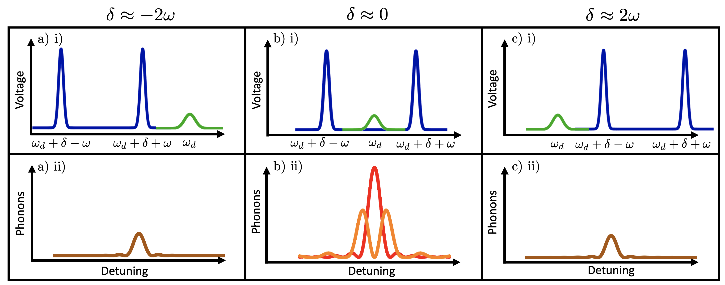
Figure 5: Illustration of spectrum sweep procedure. (a-c, i) Two quadrupole tones (blue) are swept in frequency across a weaker dipole tone (green). (a-c, ii) The resulting mean phonon number $\langle n\rangle$ produced from the corresponding interaction in (i). (a, i-ii) The interaction is primarily determined by that between the blue quadrupole tone at $\omega_{d}+\delta+\omega$ and the dipole tone at $\omega_{d}$. This interaction is phase-independent. (b, i-ii) Both quadrupole tones at $\omega_{d}+\delta\pm\omega$ interact with the dipole tone at $\omega_{d}$. The resulting interaction is phase-dependent, and can produce a resonance (red) when the phase relation satisfies $\phi_{d}-\phi_{+}=0$, where $\phi_{+}=\frac{\phi_{b}+\phi_{r}}{2}$, or an antiresonance (orange) when $\phi_{d}-\phi_{+}=\frac{\pi}{2}$. (c, i-ii) Conversely to (a), the interaction is primarily determined by that between the red quadrupole tone at $\omega_{d}+\delta-\omega$ and the dipole tone at $\omega_{d}$, and is phase-independent.

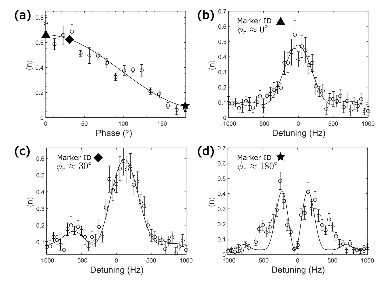
Figure 6: Phase dependence of the detuning sweeps. The phase relation between the QVSA tones fundamentally changes the lineshape of the resonance. By sweeping just $\phi_{r}$, the phase dependence is reduced to $\langle n\rangle\propto\cos^{2}{(\frac{\phi_{r}}{2})}$. (a) shows the phase sweep we performed, with three different phase locations marked by a triangle (b), a diamond (c), and a star (d). The lines are analytical expressions using (24). (d) illustrates the production of an antiresonance, which occurs when the red sideband is completely out of phase with the blue sideband (see Fig. 1(b) in the main text for a graphical representation).

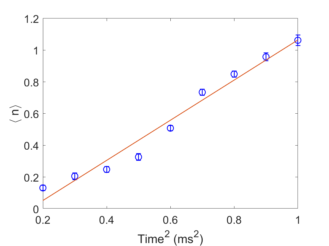
Figure 7: Quadratic heating rate of the QVSA interaction. Increasing the interaction time improves the minimum measurable signal, but is limited by the stability of the system (see Fig. 3 in the main text).

.3 Appendix B: Two Quadrupole Tones Squeezing

The effect of the quadrupole tones can be found from the interaction picture Hamiltonian from Appendix A with $V_{d}=0$:

$$H_{I}=\hbar\Omega_{q}\left(\hat{a}^{2}e^{-2i\omega t}+2\left(\hat{a}^{\dagger}\hat{a}+\frac{1}{2}\right)+\hat{a}^{\dagger 2}e^{2i\omega t}\right)\cos{\left(\left(\omega_{d}+\delta\right)t\right)}\cos{\left(\omega t\right)}$$ (13)

As before, we consider only the second order Magnus term and make a RWA approximation to find the propagator as:

$$U(t)\approx \exp\left[\frac{i\Omega_{q}^{2}t}{2}\left(\frac{\omega}{\omega_{d}^{2}-\omega^{2}}\right)(\hat{a}^{2}+\hat{a}^{\dagger 2})\right]$$ (14)

which takes the form of the squeezing operator $S(z)=\exp\left[\frac{1}{2}\left(z^{*}\hat{a}^{2}-z\hat{a}^{\dagger 2}\right)\right]$, where $z=-i\Omega_{q}^{2}(\frac{\omega}{\omega_{d}^{2}-\omega^{2}})t$.

.4 Appendix C: Derivation of Inherent Squeezing

Now suppose that the dipole tone is turned on as in Appendix A. We now reconsider the second order Magnus term with both the terms that lead to displacement as well as the terms that lead to squeezing, $A_{2}=(\alpha\hat{a}^{{\dagger}}-\alpha^{*}\hat{a})+\frac{1}{2}(z^{*}\hat{a}^{2}-z\hat{a}^{{\dagger}2})$. Note that in our experiment, $\alpha^{*}=-\alpha$ and $z^{*}=-z$. Using the Zassenhaus relation, the propagator is found as:

$$\hat{U}=S(z)D\left(\sum_{j=1}^{\infty}\frac{\imath^{j}(-1)^{j+1}\lvert\alpha\rvert\lvert z\rvert^{j-1}}{j!}\right)=S(z)D\left(\lvert\frac{\alpha}{z}\rvert(\cosh{z}+\imath\sinh{z}-1)\right)=S(z)D(\alpha^{\prime}).$$ (15)

The physical consequence of this intrinsic squeezing and displacement is the presence of a low $V_{q}$ and high $V_{q}$ regime. This is evident in Fig. 8, where $\langle n\rangle$ exhibits increasingly superlinear behavior as $V_{q}^{2}$ increases.

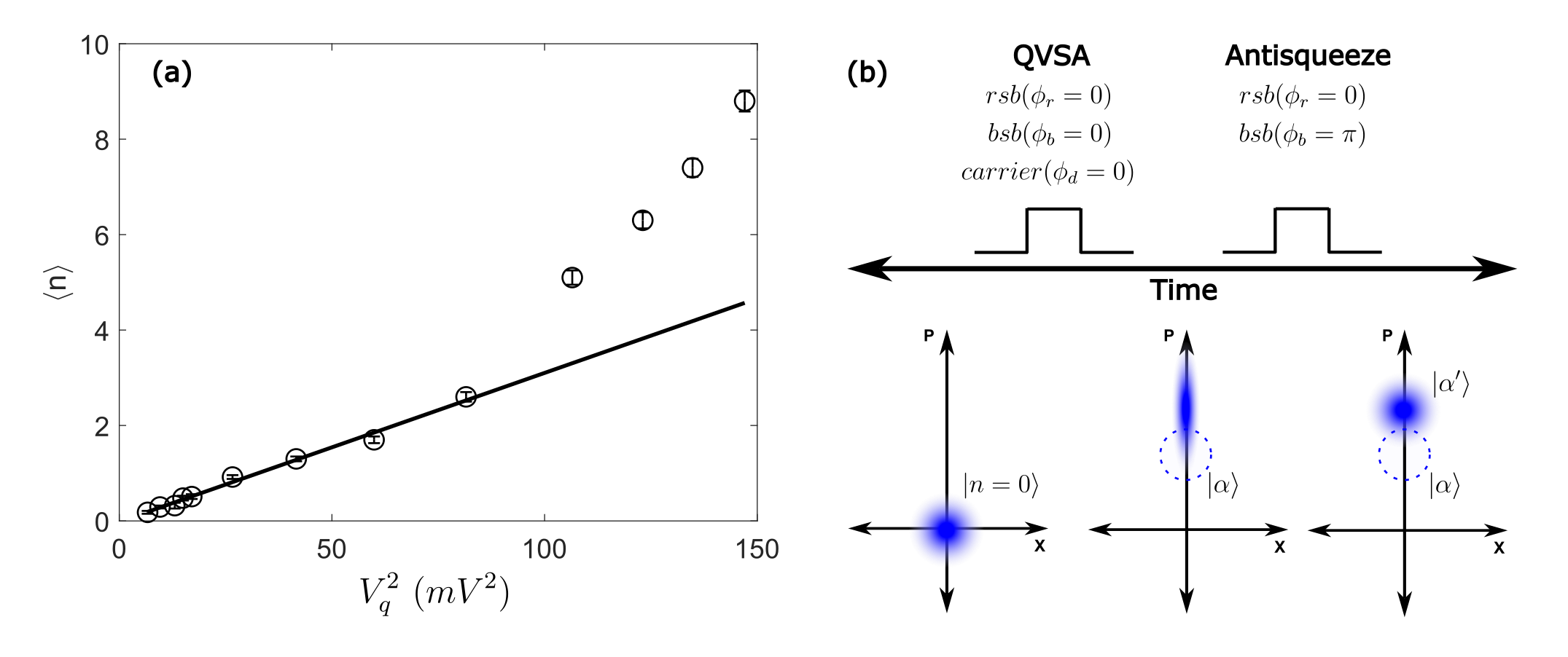
Figure 8: Intrinsic amplification at high $V_{q}$ regime. (a) Intrinsic amplification in the phonon number from high probing voltages. The line is a linear fit to the data in the low $V_{q}^{2}$ regime. The deviation of the data from the fitted line in (a) at higher $V_{q}$ illustrates the quantum behavior of this technique and that sensitivity can be further improved by operating in this regime. (b) Pulse sequence for intrinsic amplification and associated Wigner functions. The dashed lines on the bottom figures depict a pure displacement to $\ket{\alpha}$ as would be expected from the solid line in (a). The QVSA pulse is made up of a displacement operation followed by a squeeze operation, as illustrated by the colored ellipse. To convert from a squeezed state back to a coherent state $\ket{\alpha^{\prime}}$ we antisqueeze by shifting the blue sideband phase by $\pi$.

.5 Appendix D: Experimental Details

.5.1 Phase Matching

All signals for the QVSA interaction are generated using the Sinara “Phaser” Arbitrary Waveform Generator (AWG). The AWG has two coherent outputs, both of which are used to separately address a pair of quadrupolar trapping rods. Dipole signals (i.e. $\hat{x}$ terms) and quadrupole signals (i.e. $\hat{x}^{2}$ terms) can be simply generated from the same AWG by setting an inter-channel phase delay of $\pi$ and $0$, respectively. Systematic inter-channel phase delays and latencies are coarsely compensated using an oscilloscope, while fine compensation is achieved by sweeping the inter-channel phase and maximizing the measured displacement.

The relative phase of the dipole tone $\phi_{d}$ can be similarly calibrated. From (11), maximal displacement occurs when $\phi_{d}=\phi_{+}=\frac{\phi_{r}+\phi_{b}}{2}$, where $\phi_{r}$ and $\phi_{b}$ are the red and blue sideband phases, respectively. Again, we achieve this in practice by sweeping one sideband phase while keeping the other constant and maximizing the resulting displacement.

.5.2 Amplitude Matching

To calibrate the amplitudes of the quadrupole tones it would be beneficial if there was a method where we are phase independent. Luckily, as described in Fig.5, when a single quadrupole is generated at $\omega_{d}\pm\omega$ we can produce two phase-independent displacements. By measuring the displacements of the red sideband and the carrier and comparing it with the displacement from the blue sideband and the carrier, we are able to discern where the amplitudes of the sidebands are of the same strength on the electrodes. After amplitude of both quadrupole tones are matched, motional squeezed state can be produced by running at high voltage and the absolute amplitude of each tone can be figured out.

.5.3 Trapping

A quadrupole RF trap has two pairs of orthogonal electrodes, which we term the “RF” and “QVSA” electrodes. A DC voltage is applied to break the radial degeneracy, preventing phonon transfer between the resulting “RF” and “QVSA” modes. Our implementation applies QVSA signals on the “QVSA” electrodes to excite motion along the “RF” mode, which is made possible due to imperfections in trap geometry, though the effective voltage is reduced by an experimentally determined geometric factor $\kappa=\frac{1}{42}$. This is desirable since the electronics connected to the “QVSA” electrodes result in a higher motional heating rate for the “QVSA” mode.

Application of the QVSA interaction causes a shift in the trap secular frequency due to the QVSA’s use of quadrupole fields, as well as AC light shifts during readout. We empirically calibrate these shifts by scanning over the QVSA quadrupole frequencies and AOM readout frequencies and use the results to optimize our experimental parameters.

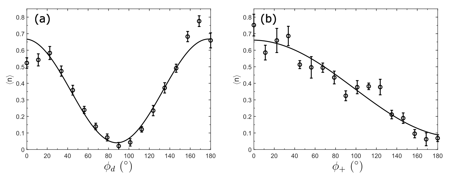
Figure 9: Phase dependence of the QVSA displacement. Displacement is maximized when $\phi_{d}=\phi_{+}$. However, since $\lvert\alpha\rvert$ depends only on the relative phase between $\phi_{d}$ and $\phi_{+}$ (see (11)), neither phase is able to be exactly determined. (a) Effect of the dipole tone phase $\phi_{d}$ on $\langle n\rangle$. (b) Effect of the relative quadrupole phase $\phi_{+}$ on $\langle n\rangle$.

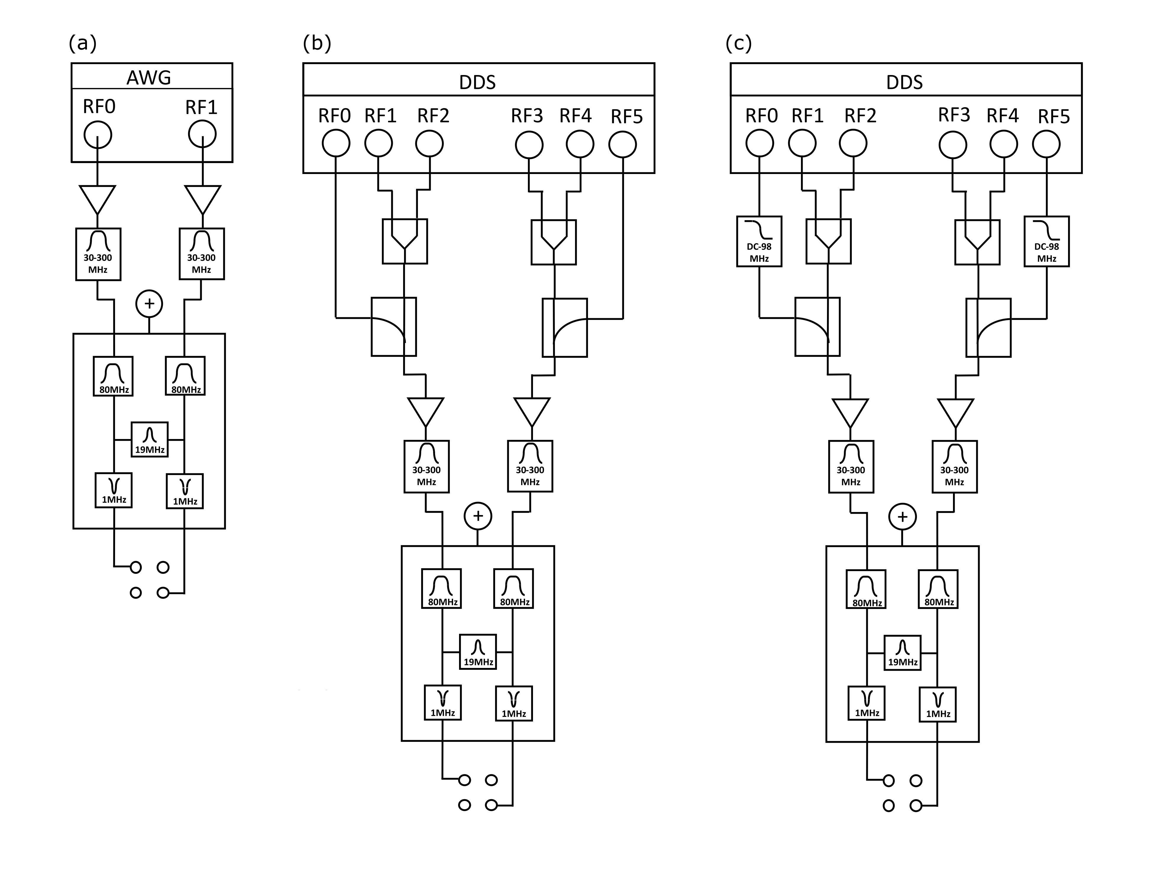
Figure 10: RF schematic of the QVSA signal generation apparatus. (a-c) Signals are amplified (Mini-Circuits ZHL-20W-13SW+) before filtering and DC biasing (used to break the radial mode degeneracy). A narrow 19 MHz band-pass functions as a diplexer to selectively short to ground any pickup from our 19 MHz trap RF, improving trap stability. (a) Configuration used for vector signal analysis. QVSA signals are generated using an Arbitrary Waveform Generator (Sinara “Phaser” Upconverter). Dipole and quadrupole fields are generated with the same AWG by setting an inter-channel phase delay of $\pi$ and $0$, respectively. (b-c) Configuration used for vector network analysis. Two banks of synchronously clocked Direct Digital Synthesizers (DDSs) (Sinara AD9910 Urukul) are used to generate the QVSA signals. This configuration allows QVSA function as a vector network analyzer (VNA) as the dipole tones can be separately passed through a Device Under Test.

.6 Appendix E: The Standard Quantum Limit

The relationship between phonon number $\langle n\rangle$ and dipole carrier detuning $\delta$ is shown in (2) of the main text and can be simplified as

$$\langle n\rangle={\lvert\alpha\rvert}^{2}{\frac{\sin^{2}(\delta T)}{(\delta T)^{2}}}$$ (16)

where $\lvert\alpha\rvert$ is the displacement amplitude in phase space and T is the QVSA interaction time. At the SQL, phonon uncertainty follows the shot noise limit, i.e. $\Delta n=\lvert\alpha\rvert\sin(\delta T)/(\delta T\sqrt{N})$, where $N$ is the number of experiments. From (16), the slope of Rabi fringes are

$$\pdv{n}{\delta}=2{\lvert\alpha\rvert}^{2}\frac{\delta T\sin{\left(\delta T\right)}\cos{\left(\delta T\right)}-\sin^{2}\left(\delta T\right)}{\delta(\delta T)^{2}}$$ (17)

The frequency uncertainty of the dipole tone $\Delta\delta$ is therefore

$$\Delta\delta =\frac{\Delta n}{\pdv{n}{\delta}}$$

$$=\frac{\left(\delta T\right)^{2}}{\delta T^{2}\cos{\left(\delta T\right)}-T\sin{\left(\delta T\right)}}\frac{1}{2\lvert\alpha\rvert\sqrt{N}}.$$ (18)

Unlike in Ramsey spectroscopy, where the SQL is independent of detuning [17], the Allan deviation for Rabi spectroscopy involves measurement of two detuning points near the half-width, where there is a good trade-off between the signal-to-noise ratio (SNR) and the sensitivity. Under these conditions, $\sin(\delta T)/(\delta T)=1/\sqrt{2}$. The SQL for the dipole frequency is finally

$$\Delta\delta=2\pi\frac{0.209}{\lvert\alpha\rvert T\sqrt{N}}$$ (19)

The relationship between the phonon number $\langle n\rangle$ and the dipole tone phase $\phi_{d}$ can be expressed as:

$$\langle n\rangle=\lvert\alpha\rvert^{2}\cdot\sin^{2}(\theta+2\phi_{d}),$$ (20)

where $\theta$ is the variation of the initial phase. Similarly, the dipole tone phase uncertainty follows $\Delta\phi_{d}=\frac{\Delta n}{\pdv{n}{\phi_{d}}}$.

At the SQL, $\Delta n=\lvert\alpha\rvert\cdot\sin(\theta+2\phi_{d})/\sqrt{N}$; $\pdv{n}{\phi_{d}}=4{\lvert\alpha\rvert}^{2}\sin(\theta+2\phi_{d})\cos(\theta+2\phi_{d})$. Then,

$$\Delta\phi_{d} =\frac{\Delta n}{\pdv{n}{\phi_{d}}}$$

$$=\frac{1}{\cos(\theta+2\phi_{d})}\frac{1}{4\lvert\alpha\rvert\sqrt{N}}.$$ (21)

Similarly, for the Allan deviation measurement, two points are measured at the detuning corresponding to half width (i.e. $\cos(\theta+2\phi_{d})=1/\sqrt{2}$). Then,

$$\Delta\phi_{d}=\frac{1}{2\lvert\alpha\rvert\sqrt{2N}}$$ (22)

.7 Appendix F: Motional detection

In order to determine the strength of the displacement from the QVSA, we measure the mean phonon number of the ion through two methods.

.7.1 Sideband ratio

For the sideband ratio technique, fluorescence is read out after the 729nm laser scans over points on the red and blue motional sidebands for time $t_{\pi}$, where $t_{\pi}$ is roughly the $\pi$-pulse time of the first optical blue sideband transition. The ratio of the red and blue sideband D-state populations is then converted to a displacement assuming a coherent state (Fig. 11(a, e)). This technique works well when $\langle n\rangle<1$, but becomes non-injective and inefficient when $\langle n\rangle>1$.

To extract the displacement due to the QVSA interaction, we apply the sideband ratio technique while scanning the symmetric detuning of the quadrupole tones from the dipole tone, i.e. we scan $\delta_{q}=\lvert\omega_{d}-\omega_{q}\rvert$ across the secular frequency $\omega$ (Fig. 11(a-d)). The resulting profile is fitted with a sinc² function to extract the displacement (Fig. 11(e)). However, for Allan deviations, we instead measure only a single point at the secular frequency resonance where $\delta_{q}=\omega$.

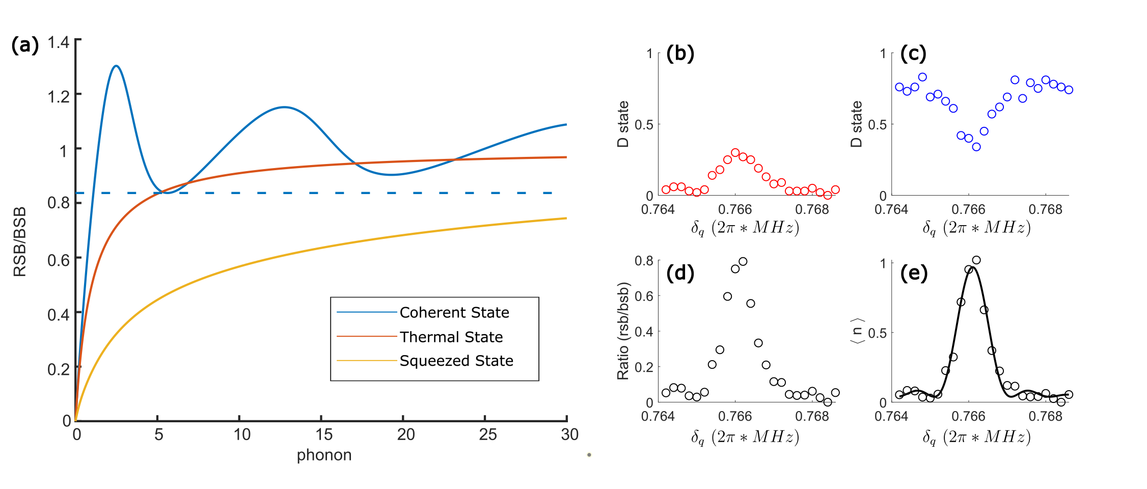
Figure 11: Measurement of $\langle n\rangle$ via the sideband ratio technique. (a) Conversion of the sideband ratio to a mean phonon number for different motional states. We assume that the sidebands are interrogated for time $t_{\pi}\approx\pi/\Omega_{01}$, where $\Omega_{01}$ is the Rabi frequency for the $\ket{S,n=0}$ to $\ket{D,n=1}$ transition. (b) and (c) are example distributions of the D-state populations via red and blue sidebands alongside frequency $\lvert\omega_{q}-\omega_{d}\rvert$ scanned across secular frequency, of which $\omega_{q}$ is the frequency of one of quadrupole tones. (d) shows the ratio of the sidebands, which we need to be below 0.829 to insure the correct phonon number, shown in (e).

.7.2 Blue sideband (BSB) Rabi flopping

Blue sideband Rabi flopping [18] is the preferred technique when $\langle n\rangle>1$, but is more susceptible to qubit decoherence. By fitting the blue sideband Rabi oscillations, mean phonon and populations in each Fock state can be extracted [19]. We use this method specifically for quantum amplification data, which often results in $\langle n\rangle>1$. A sample pulse sequence including quantum amplification is shown in Fig. 13. Additionally, this technique is helpful when extracting $\langle n\rangle$ for squeezed states due to the inefficiency of the sideband ratio technique for squeezed states (Fig. 12). Our blue sideband oscillations have a coherence time $\approx 500\mu$s, which is limited by the servo bump of our 729nm laser and magnetic field fluctuations.

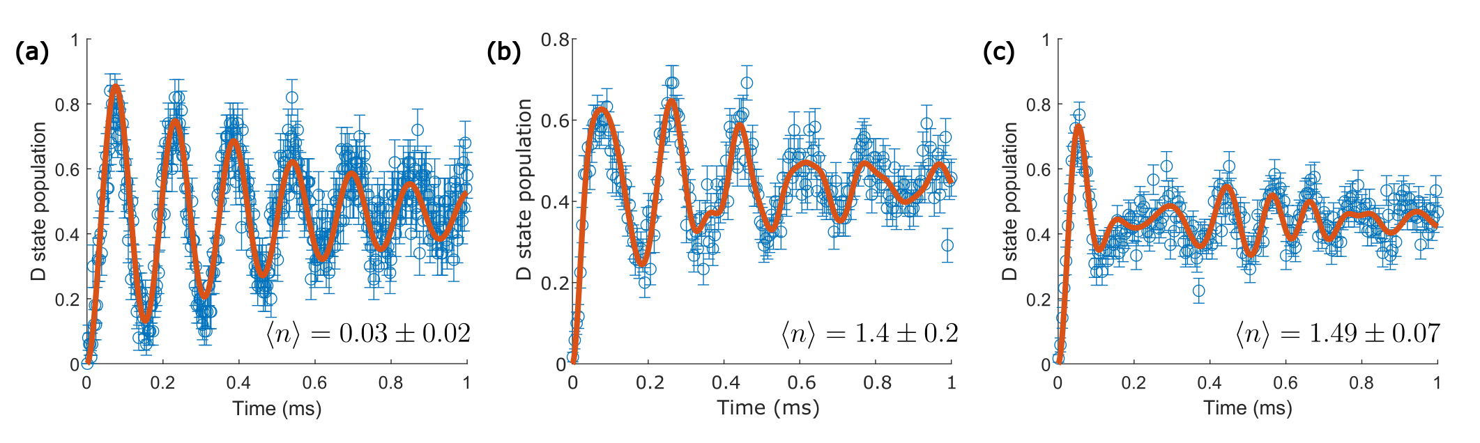
Figure 12: Blue sideband (BSB) Rabi oscillation for different motional states. The decoherence time $t_{dec}$ is roughly $500$ ms, and the Rabi frequency on resonance with the qubit transition $\Omega_{00}$ is $2\pi\cdot 120$ kHz. (a) BSB Rabi oscillations after sideband cooling to the motional ground state and fitted using a thermal state. (b) BSB Rabi oscillations for a squeezed state, which is prepared through parametric modulation of the trap potential at twice the secular frequency. (c) BSB Rabi oscillations for a coherent state produced using the QVSA interaction.

.8 Appendix G: Vector Network Analysis via QVSA

We demonstrate the functionality of our technique for vector network analysis by measuring the transfer function of a commercial low-pass filter (Mini-Circuits SLP-100+). The RF configuration used for these measurements is shown in Fig. 10(b-c). For normalization, we first measure the transfer function of the dipole tone without the Device Under Test (DUT) (i.e. the low-pass filters) in place (Fig. 10(b)). At each frequency, the RSB phase $\phi_{r}$ is scanned, and the resulting displacement is fitted to eq. 2 in main text to extract the voltage and phase of the signal coupled onto the electrodes. This procedure is then repeated with the DUT in place (Fig. 10 (c)). The transfer function of the DUT can then be given by subtracting the normalization data from the DUT data.

The original intent of this technique was to calibrate the transmission of RF tones used to drive a molecular transition [12]. The insertion loss and phase response was determined from 20 MHz to 300 MHz using the same procedure above. The frequency range is limited by our AWG. We compare our results against that measured using a commercial network analyzer in Fig. 14. Evidently, both measurements demonstrate a general agreement but fail to agree within 3 dB for almost the entirety of the scanned range. This is a characteristic example of the difficulty of accurately calibrating qubit signals. Unlike standard elements (e.g. our low-pass filter), the ion trap is inaccessible and cannot be directly interfaced without changing the measurement conditions and the consequent results. For example, our VNA measurements use a capacitive pickoff close to the trap as the output port, as opposed to the trap electrode itself. This example demonstrates the power of our QVSA technique for generating in situ measurements.

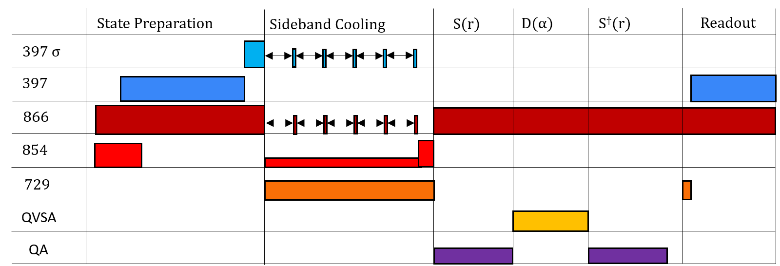
Figure 13: Pulse sequence for the QVSA with Quantum Amplification. The ion is Doppler cooled and optically pumped into the $\ket{{}^{2}S_{\frac{1}{2}},m_{J}=-\frac{1}{2}}$ state. Continuous sideband cooling subsequently prepares the ion near the ground motional state $\ket{n=0}$. Quantum Amplification is achieved by preparing the ion in a squeezed state before applying the QVSA pulse, which amplifies the displacement and minimizes uncertainty along the squeezing axis. The squeezing is then reversed via an anti-squeezing pulse, returning the ion to a coherent state.

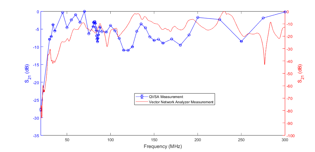
Figure 14: Insertion loss of the ion trap system measured using the QVSA and a commercial vector network analyzer (VNA). Blue (red) data shows the insertion loss measured by the QVSA (VNA).
The failure of the traditional ex situ measurement is apparent.

References

- Wolf et al. [2019] F. Wolf, C. Shi, J. C. Heip, M. Gessner, L. Pezzè, A. Smerzi, M. Schulte, K. Hammerer, and P. O. Schmidt, Motional fock states for quantum-enhanced amplitude and phase measurements with trapped ions, Nature Communications 10, 2929 (2019).
- McCormick et al. [2019] K. C. McCormick, J. Keller, S. C. Burd, D. J. Wineland, A. C. Wilson, and D. Leibfried, Quantum-enhanced sensing of a single-ion mechanical oscillator, Nature 572, 86 (2019).
- Burd et al. [2019] S. C. Burd, R. Srinivas, J. J. Bollinger, A. C. Wilson, D. J. Wineland, D. Leibfried, D. H. Slichter, and D. T. C. Allcock, Quantum amplification of mechanical oscillator motion, Science 364, 1163 (2019), doi: 10.1126/science.aaw2884.
- Gilmore et al. [2017] K. A. Gilmore, J. G. Bohnet, B. C. Sawyer, J. W. Britton, and J. J. Bollinger, Amplitude sensing below the zero-point fluctuations with a two-dimensional trapped-ion mechanical oscillator, Phys. Rev. Lett. 118, 263602 (2017).
- Gilmore et al. [2021] K. A. Gilmore, M. Affolter, R. Lewis-Swan, D. Barberena, E. Jordan, A. Rey, and J. J. Bollinger, Quantum-enhanced sensing of displacements and electric fields with two-dimensional trapped-ion crystals, Science 373, 673 (2021).
- Milne et al. [2021] A. Milne, C. Hempel, L. Li, C. Edmunds, H. Slatyer, H. Ball, M. Hush, and M. Biercuk, Quantum oscillator noise spectroscopy via displaced cat states, Phys. Rev. Lett. 126, 250506 (2021).
- Keller et al. [2021] J. Keller, P.-Y. Hou, K. C. McCormick, D. C. Cole, S. D. Erickson, J. J. Wu, A. C. Wilson, and D. Leibfried, Quantum harmonic oscillator spectrum analyzers, Phys. Rev. Lett. 126, 250507 (2021).
- Burd et al. [2021] S. C. Burd, R. Srinivas, H. M. Knaack, W. Ge, A. C. Wilson, D. J. Wineland, D. Leibfried, J. J. Bollinger, D. T. C. Allcock, and D. H. Slichter, Quantum amplification of boson-mediated interactions, Nature Physics 17, 898 (2021).
- Burd et al. [2023] S. C. Burd, H. M. Knaack, R. Srinivas, C. Arenz, A. L. Collopy, L. J. Stephenson, A. C. Wilson, D. J. Wineland, D. Leibfried, J. J. Bollinger, D. T. C. Allcock, and D. H. Slichter, Experimental speedup of quantum dynamics through squeezing (2023), arXiv:2304.05529 [quant-ph] .
- Ge et al. [2019] W. Ge, B. C. Sawyer, J. W. Britton, K. Jacobs, J. J. Bollinger, and M. Foss-Feig, Trapped ion quantum information processing with squeezed phonons, Phys. Rev. Lett. 122, 030501 (2019).
- Roos et al. [1999] C. Roos, T. Zeiger, H. Rohde, H. C. Nägerl, J. Eschner, D. Leibfried, F. Schmidt-Kaler, and R. Blatt, Quantum state engineering on an optical transition and decoherence in a paul trap, Phys. Rev. Lett. 83, 4713 (1999).
- Hudson and Campbell [2021] E. R. Hudson and W. C. Campbell, Laserless quantum gates for electric dipoles in thermal motion, Phys. Rev. A 104, 042605 (2021).
- Note [1] Two quadrupole sidebands separated by 2 can form a squeeze operator. Once 8.4 Vms, the squeezing becomes significant. We discuss operation in this intrinsic squeezing regime in what follows.
- Natarajan et al. [1995] V. Natarajan, F. DiFilipo, and D. Pritchard, Classical squeezing of an oscillator for subthermal noise poperartion, Phys. Rev. Lett. 74, 2855 (1995).
- Hempel et al. [2013] C. Hempel, B. P. Lanyon, P. Jurcevic, R. Gerritsma, R. Blatt, and C. F. Roos, Entanglement-enhanced detection of single-photon scattering events, Nature Photonics 7, 630 (2013).
- Gely et al. [2023] M. F. Gely, J. M. Litarowicz, A. D. Leu, and D. M. Lucas, In-situ characterization of qubit drive-phase distortions (2023), arXiv:2309.14703 [quant-ph] .
- Itano et al. [1993] W. M. Itano, J. C. Bergquist, J. J. Bollinger, J. M. Gilligan, D. J. Heinzen, F. L. Moore, M. G. Raizen, and D. J. Wineland, Quantum projection noise: Population fluctuations in two-level systems, Phys. Rev. A 47, 3554 (1993).
- Meekhof et al. [1996] D. M. Meekhof, C. Monroe, B. E. King, W. M. Itano, and D. J. Wineland, Generation of nonclassical motional states of a trapped atom, Phys. Rev. Lett. 76, 1796 (1996).
- Lo et al. [2015] H.-Y. Lo, D. Kienzler, L. de Clercq, M. Marinelli, V. Negnevitsky, B. C. Keitch, and J. P. Home, Spin–motion entanglement and state diagnosis with squeezed oscillator wavepackets, Nature 521, 336 (2015).