[aff1] organization = Zhejiang Institute of Modern Physics, School of Physics, Zhejiang University, addressline = 866 Yuhangtang Road, postcode = 310027, city = Hangzhou, country = China [aff2] organization = School of Physics, Peking University, addressline = 209 Chengfu Road, postcode = 100871, city = Beijing, country = China [aff3] organization = Center for High Energy Physics, Peking University, addressline = 209 Chengfu Road, postcode = 100871, city = Beijing, country = China [aff4] organization = Max-Planck-Institut für Physik, addressline = Boltzmannstr. 8, postcode = 85748, city = Garching, country = Germany

Reclassifying Feynman Integrals as Special Functions

Feynman integrals (FIs) serve as fundamental components of perturbative quantum field theory. The study of FI is important both for exploring the mysteries of quantum field theories and for their phenomenological applications, especially in particle physics. Extensive efforts have been dedicated to the pursuit of analytical calculations of FIs, aiming to express them as linear combinations of special functions. This approach, however, faces formidable challenges due to the involvement of relatively less explored special functions, such as those defined on elliptic curves [1] and Calabi-Yau manifolds [2]. Conversely, a different avenue for tackling FIs involves utilizing numerical differential equations [3] and the auxiliary mass flow method [4, 5, 6, 7, 8], which in principle enables the computation of any FI to arbitrary precision. Consequently, a shift in perspective can be adopted by considering FIs as a new class of special functions, the study of which can also help to understand those relatively less explored special functions. To advance this line of inquiry, there is a need for a more comprehensive investigation of the properties of FIs.

Space of special functions. The question of which kind of transcedental numbers or special functions could appear in the scattering amplitudes was posed long ago. In recent years, the differential equation method [3] has become one of the most important tools to tackle this problem.

A $L$-loop FI with $N$ propagators is usually defined as

$$I_{\vec{\nu}}=\int\prod_{i=1}^{L}\frac{\mathrm{d}^{d}l_{i}}{i\pi^{d/2}}\prod_{a=1}^{N}\frac{1}{{\cal D}_{a}^{\nu_{a}}},$$ (1)

where $l_{i}$ are $d$-dimensional loop momenta to be integrated out, and ${\cal D}_{a}$ are propagators which are polynomials of masses and dot products of momenta. $\nu_{a}$ are integer powers of the propagators. A FI is an analytic function of the kinematic invariants $s_{i}$, which can be either scalar products of external momenta or masses in the propagators. It has been proven that for a given set of ${\cal D}_{a}$, any $I_{\vec{\nu}}$ can be written as a linear combination of a finite set of basis $I_{i}$, called master integrals, using FI reduction technique [9, 10],

$$I_{\vec{\nu}}=\sum_{i=1}^{M}c_{\vec{\nu},i}I_{i},$$ (2)

where $M$ is finite and $c_{\vec{\nu},i}$ are rational functions of kinematic variables and space-time dimension $d$. Differentiate $I_{i}$ with respect to kinematic invariants and then reduce back to the same basis, we immediately realize that the FIs $I_{i}$ satisfy a system of differential equations

$$\frac{\partial}{\partial s_{i}}\bm{I}(\epsilon,\vec{s}~{})=\bm{A}_{i}(\epsilon,\vec{s}~{})\bm{I}(\epsilon,\vec{s}~{}),$$ (3)

where $\epsilon$ is defined through $d=4-2\epsilon$, and $\bm{A}_{i}$ are matrices whose elements are rational functions of $\epsilon$ and $\vec{s}$.

In some cases, by choosing proper master integrals $\bm{I}^{\prime}$, the differential equations can be put into the so-called “canonical form” [11], where the dependency of $\epsilon$ factorizes

$$\frac{\partial}{\partial s_{i}}\bm{I}^{\prime}(\epsilon,\vec{s}~{})=\epsilon\bm{A}^{\prime}_{i}(\vec{s}~{})\bm{I}^{\prime}(\epsilon,\vec{s}~{}).$$ (4)

The resulting equation often takes a very compact form, and the analytic solution at each order of $\epsilon$ expansion can be written down directly using iterated integrals. In the simplest case, these iterated integrals can be defined as multiple polylogarithms [12]. The rich algebraic structures of multiple polylogarithms allow us to simplify the expression considerably using the symbol technique [13] or directly write down an ansatz to the final result of the FIs and then fix the unknown coefficients with the help of other knowledge we have about the integrals. Many cutting-edge phenomenological problems have been solved by this strategy in recent years.

More generally, one can cast the system of first-order differential equations into a differential operator acting on one of the master integrals. After factorizing this differential operator into a product of simpler differential operators, information about the special functions involved in the solution can be obtained by studying each individual factor [14]. If all the factors are first-order, we would expect that the solution can be written as multiple polylogarithms. If we encounter an irreducible second-order differential operator, the iterated integral solution would contain an elliptic curve. From this perspective, the space of special functions can be arbitrarily complicated if there is no strong constraint on the form of the differential operator. Indeed, besides multiple polylogarithms and elliptic curves, people have discovered differential operators associated with algebraic curves with higher genus and more complicated geometric objects like Calabi-Yau manifolds [2]. For special functions beyond multiple polylogarithms, it is currently not only hard to take advantage of the symbol technique, but also challenging to compute numerical results at given kinematic points. This is a hot topic under study currently.

Semi-analytical computation. The auxiliary mass flow method was first proposed in 2017 [4] and developed in the past few years [5, 6, 7]. Now it can in principle calculate any FI to arbitrary precision, giving sufficient computational power. The method has been implemented in the computer program AMFlow [8], which can calculate FIs fully automatically. In this method, we usually replace one inverse propagator ${\cal D}_{a}$ in Eq. (1) by ${\cal D}_{a}+i\eta$ and then setup differential equations of the modified master integrals $\widetilde{\bm{I}}$ with respect to the “auxiliary mass” term $\eta$,

$$\frac{\partial}{\partial\eta}\widetilde{\bm{I}}(\epsilon,\vec{s}~{},\eta)=\widetilde{\bm{A}}(\epsilon,\vec{s}~{},\eta)\widetilde{\bm{I}}(\epsilon,\vec{s}~{},\eta),$$ (5)

which can be achieved by using FIs reduction technique. If a boundary condition for the differential equations is also known, the original FIs ${\bm{I}}$ can be obtained by solving these ordinary differential equations numerically.

Fortunately, the boundary condition at $\eta\to\infty$ can always be obtained. In this limit, the modified master integrals become linear combinations of three kinds of FIs: The first kind is obtained by removing the inverse propagator ${\cal D}_{a}$, whose calculation becomes a simpler problem with the same structure and can be solved recursively; The second kind is factorized FIs, which are much simpler, can be solved recursively too; And the last kind of FIs are one-mass vacuum FIs, which have no external momentum dependence. To calculate the last kind of FIs, we relate them to FIs with two external legs but having one less loop, which can again be calculated by using the auxiliary mass flow method above. By applying the method recursively, any FI can be completely determined, with only input from FIs reduction which involves purely linear algebraic operations.

The AMFlow method allows conveniently evaluating FIs at any kinematic point in the kinematic space. For phenomenological applications, one may simply populate the whole kinematic space by evaluating each individual kinematic point with the AMFlow method, first fixing the kinematic variables and then moving along the direction of the auxiliary parameter to find the integral value. This approach is easy to implement and easy to parallelize, but it ignores the fact that the value of FIs at two nearby kinematic points often changes smoothly, which makes its efficiency suboptimal.

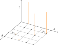
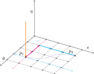
Figure 1: Comparison of different evaluation strategies. (a) Using AMFlow point by point; (b) Using AMFlow to provide a boudary condition and then using differential equations with respect to kinematic variables.

The information about how Feyman integrals change in the kinematic space is already encoded in the differential equation with respect to the kinematic variables that span the space. Thus, once we know the value of the integrals at one kinematic point, it is much more convenient to move directly from one point to another in the kinematic space than to move along the extra dimension of the auxiliary parameter every single time.

The difference between these two approaches can be clearly seen in Fig. 1. In this example, the kinematic space is spanned by the center-of-mass energy $s$ and scattering angle $\theta$, while the auxiliary mass parameter used by AMFlow is denoted as $\eta$. In the first approach, each point in the kinematic space is evaluated along the $\eta$ direction. While in the second approach, $p_{1}$ is first evaluated with the help of AMFlow, and $p_{2}$ is then evaluated using the differential equation along the $\theta$ direction, and finally along the $s$ direction. One could also move along any curve in the kinematic space, provided that the correct analytic continuation is used.

Solving differential equations in kinematic space also opens up alternative ways of evaluating the points. For one-dimensional kinematic space, one may consider covering the kinematic space with a set of series solutions, which would allow efficient evaluation of FIs anywhere in the kinematic space. For lower-dimensional kinematic space, it is possible to build a grid of series solutions. While for higher-dimensional kinematic space, the rapid increase in the grid size suggests that importance sampling would be a more efficient strategy. Therefore, by combining the auxiliary mass flow method and numerical differential equations with respect to kinematic variables, FIs can be calculated fully systematically and efficiently.

Feynman integrals as special functions. Although FIs cannot be expressed as well-studied special functions, they can be calculated systematically and efficiently using the AMFlow method in combination with differential equations in the kinematic space, as we have discussed above. Therefore, it is constructive to define FIs as a new class of special functions (or transcedental numbers if there is no kinematic variable in FIs). The so-called special functions often exhibits the following traits:

1. Having both integral and differential representations;

2. Well-studied asymptotic behavior around singularities and branch cuts;

3. Availability of series expansions everywhere;

4. Satisfying certain algebraic relations among them.

These traits facilitate the exploration of global and local properties of the function space, and also provide efficient evaluation methods. We will show that FIs can indeed satisfy all these points, although better strategies for many aspects are still needed.

1) FIs have integral representations by definition, and master integrals, which are bases of FIs, have closed differential equations with respect to kinematic variables. Considering also that boundary conditions can always be obtained through the AMFlow method, the first condition is satisfied. Nevertheless, it should be pointed out that there is no differential equation with respect to $\epsilon$, therefore $\epsilon$ should be thought as a parameter instead of an argument for the special functions. By expanding $\epsilon$ around the origin,

$$\bm{I}(\epsilon,\vec{s}~{})=\sum_{i}\bm{I}^{(i)}(\vec{s}~{})\epsilon^{i},$$ (6)

the coefficients can also be defined as special functions, and original FIs serve as generating functions for these special functions.

2) The singularities of FIs are determined by Landau equations, but these equations are usually very hard to solve. Alternatively, singularities can be identified as a subset of poles in differential equations, say $A_{i}$ in Eq. (3). Spurious poles can be ruled out by inspecting their monodromy groups, as those groups associated with spurious poles act trivially on master integrals. Branch cuts are usually identified by studying the Feynman prescription $i0^{+}$ in propagators, although this is not always an easy way to tackle the problem, especially when some of the propagators are replaced by delta functions. The bottom line is that we can use AMFlow to compute some points around a branch point, so that we can fully determine the asymptotic expansion at the point and thus determine the corresponding branch cut.

3) With differential representation, boundary conditions and singular structures discussed above, we can obtain series expansion at any desired point by analytic continuation.

4) Relations among FIs have been explored by the means of integration by parts (IBP) identities. However, it is not yet clear whether IBP identities exhausted all possibilities. Furthermore, there can be more relations among coefficients after $\epsilon$ expansion shown in Eq. (6), as hinted by the study of multiple polylogarithms. Unfortunately, there is currently no efficient way to identify these relations. As AMFlow can compute the coefficients to high precision, we can at least explore their relations by PSLQ algorithm.

Outlook. We have demonstrated that, thanks to the input from AMFlow, it is feasible to define FIs as a novel class of special functions. Several crucial avenues for further exploration emerge in this direction:

• The development of an efficient technique for determining singularities and branch cuts is essential.

• A refinement of the methodology for choosing master integrals is imperative. This process should be sufficiently general to apply across diverse cases, resulting in a simple matrix $\bm{A}(\epsilon,\vec{s})$ in Eq.(3), conducive to efficient numerical computation.

• A systematic approach to exploring relations between coefficients in the $\epsilon$ expansion is warranted.

Furthermore, exploring connections between FIs and established special functions can facilitate a deeper understanding of the later unique mathematical entities. Finally, we would like to point out that FI reduction is the foundation of the differential equation method and AMFlow method, thus enhancing its efficiency is crucial to the whole story.

Conflict of interest.

The authors declare that they have no conflict of interest.

Acknowledgements.

The work was supported in part by the National Natural Science Foundation of China (Grants No. 11975029, No. 12325503), the National Key Research and Development Program of China under Contracts No. 2020YFA0406400, and the China Postdoctoral Science Foundation (Grants No. 2023M733123, No. 2023TQ0282).

References

- [1] S. Laporta and E. Remiddi, Analytic treatment of the two loop equal mass sunrise graph, Nucl. Phys. B 704 (2005) 349–386 [hep-ph/0406160] [InSPIRE].
- [2] A. Klemm, C. Nega, and R. Safari, The -loop Banana Amplitude from GKZ Systems and relative Calabi-Yau Periods, JHEP 04 (2020) 088 [arXiv:1912.06201] [InSPIRE].
- [3] E. Remiddi, Differential equations for Feynman graph amplitudes, Nuovo Cim. A 110 (1997) 1435–1452 [hep-th/9711188] [InSPIRE].
- [4] X. Liu, Y.-Q. Ma, and C.-Y. Wang, A Systematic and Efficient Method to Compute Multi-loop Master Integrals, Phys. Lett. B 779 (2018) 353–357 [arXiv:1711.09572] [InSPIRE].
- [5] X. Liu, Y.-Q. Ma, W. Tao, and P. Zhang, Calculation of Feynman loop integration and phase-space integration via auxiliary mass flow, Chin. Phys. C 45 (2021) 013115 [arXiv:2009.07987] [InSPIRE].
- [6] X. Liu and Y.-Q. Ma, Multiloop corrections for collider processes using auxiliary mass flow, Phys. Rev. D 105 (2022) L051503 [arXiv:2107.01864] [InSPIRE].
- [7] Z.-F. Liu and Y.-Q. Ma, Determining Feynman Integrals with Only Input from Linear Algebra, Phys. Rev. Lett. 129 (2022) 222001 [arXiv:2201.11637] [InSPIRE].
- [8] Z.-F. Liu and Y.-Q. Ma, Automatic computation of Feynman integrals containing linear propagators via auxiliary mass flow, Phys. Rev. D 105 (2022) 074003 [arXiv:2201.11636] [InSPIRE].
- [9] K. G. Chetyrkin and F. V. Tkachov, Integration by Parts: The Algorithm to Calculate beta Functions in 4 Loops, Nucl. Phys. B 192 (1981) 159–204 [InSPIRE].
- [10] A. V. Smirnov and A. V. Petukhov, The Number of Master Integrals is Finite, Lett. Math. Phys. 97 (2011) 37–44 [arXiv:1004.4199] [InSPIRE].
- [11] J. M. Henn, Multiloop integrals in dimensional regularization made simple, Phys. Rev. Lett. 110 (2013) 251601 [arXiv:1304.1806] [InSPIRE].
- [12] A. B. Goncharov, Multiple polylogarithms, cyclotomy and modular complexes, arXiv e-prints (May, 2011) arXiv:1105.2076 [arXiv:1105.2076] [InSPIRE].
- [13] A. B. Goncharov, M. Spradlin, C. Vergu, and A. Volovich, Classical Polylogarithms for Amplitudes and Wilson Loops, Phys. Rev. Lett. 105 (2010) 151605 [arXiv:1006.5703] [InSPIRE].
- [14] L. Adams, E. Chaubey, and S. Weinzierl, Simplifying Differential Equations for Multiscale Feynman Integrals beyond Multiple Polylogarithms, Phys. Rev. Lett. 118 (2017) 141602 [arXiv:1702.04279] [InSPIRE].
- [15] J. Écalle, Les fonctions résurgentes: (en trois parties). Université de Paris-Sud, Département de Mathématique, Bât. 425, 1981.