1
One of the most fundamental elements in fluid mechanics are the fluid
filaments. These are structures around which vorticity tends to concentrate.
Their formation, structure and evolution has been a central theme since the
early days of fluid dynamics and the main results bear the names of
Helmholtz, Lord Kelvin, Kirchhoff, etc (see the classical book by Saffman
[1 ] for a general overview or the book by Darrigol [2 ] for a
historical perspective). When a vortex filament is curved and its motion
affected by the velocity field created by itself, one could in principle
think of a closed-form equation to describe the evolution of the filament.
When the flow is inviscid, the velocity field is given by the Biot-Savart
law applied to the vorticity. This yields a singular integral and an
infinite velocity field at the filament. By replacing the zero-thickness
filament by a filament of radius ε 𝜀 \varepsilon
𝐯 = − Γ 4 π κ ( s , t ) ( log ε ) 𝐛 ( s , t ) + O ( 1 ) , 𝐯 Γ 4 𝜋 𝜅 𝑠 𝑡 𝜀 𝐛 𝑠 𝑡 𝑂 1 \mathbf{v}=-\frac{\Gamma}{4\pi}\kappa(s,t)(\log\varepsilon)\mathbf{b}(s,t)+O(1), (1)
where Γ Γ \Gamma κ ( s , t ) 𝜅 𝑠 𝑡 \kappa(s,t) s 𝑠 s 𝐛 ( s , t ) 𝐛 𝑠 𝑡 \mathbf{b}(s,t) O ( 1 ) 𝑂 1 O(1) 1 [4 ] and has produced hundreds of studies on existence,
uniqueness and properties of the solutions in relation with the physical
situations that the equation intends to model. Obvious problems with the
binormal flow are the following: LIA is an ad hoc assumption that can only
be justified as leading order for a thin vortex tube in inviscid flow and it
is still unclear what is the role of vortex filaments and the binormal flow
dynamics in the case of viscous flows. Nevertheless, there is nowadays
overwhelming evidence that binormal flow is connected to observed physical
phenomena such as the motion of vortex rings or the oscillation of perturbed
vortex rings [5 ] , [7 ] . In the case of Euler flows, the existence
of vortex rings with a core of finite thickness and moving with constant
velocity was proved by Fraenkel [14 ] and important progress has been
made recently to prove the existence of travelling helices [15 ] and
leapfrogging rings [16 ] , for instance. The more general question on
whether the binormal flow dynamics represents the evolution of a vortex
filament of thickness ε 𝜀 \varepsilon [10 ] under some hypothesis.
A vortex filament may be considered as a singular initial data for the
vorticity in the form
𝝎 ( 𝐱 , 0 ) = Γ 2 π δ G 𝐭 ( s , 0 ) , 𝝎 𝐱 0 Γ 2 𝜋 subscript 𝛿 𝐺 𝐭 𝑠 0 \bm{\omega}(\mathbf{x},0)=\frac{\Gamma}{2\pi}\delta_{G}\mathbf{t}(s,0), (2)
where δ G subscript 𝛿 𝐺 \delta_{G} G 𝐺 G Γ Γ \Gamma 𝐭 ( s , 0 ) 𝐭 𝑠 0 \mathbf{t}(s,0) ν 𝜈 \nu
∂ 𝝎 ∂ t + 𝐯 ⋅ ∇ 𝝎 − 𝝎 ⋅ ∇ 𝐯 − ν Δ 𝝎 = 0 , 𝝎 𝑡 ⋅ 𝐯 ∇ 𝝎 ⋅ 𝝎 ∇ 𝐯 𝜈 Δ 𝝎 0 \frac{\partial\bm{\omega}}{\partial t}+\mathbf{v}\cdot\nabla\bm{\omega}-\bm{\omega}\cdot\nabla\mathbf{v}-\nu\Delta\bm{\omega}=0, (3)
where 𝐯 𝐯 \mathbf{v}
𝐯 ( 𝐱 , t ) = K ∗ 𝝎 ( 𝐱 , t ) ≡ 1 4 π ∫ 𝝎 ( 𝐱 ′ , t ) × ( 𝐱 − 𝐱 ′ ) | 𝐱 − 𝐱 ′ | 3 𝑑 𝐱 ′ . 𝐯 𝐱 𝑡 ∗ 𝐾 𝝎 𝐱 𝑡 1 4 𝜋 𝝎 superscript 𝐱 ′ 𝑡 𝐱 superscript 𝐱 ′ superscript 𝐱 superscript 𝐱 ′ 3 differential-d superscript 𝐱 ′ \mathbf{v}(\mathbf{x},t)=K\ast\bm{\omega}(\mathbf{x},t)\equiv\frac{1}{4\pi}\int\frac{\bm{\omega}(\mathbf{x}^{\prime},t)\times(\mathbf{x}-\mathbf{x}^{\prime})}{\left|\mathbf{x}-\mathbf{x}^{\prime}\right|^{3}}d\mathbf{x}^{\prime}. (4)
Giga and Miyakawa, in a seminal paper [3 ] , prove the existence of weak
solutions with singular initial data. This includes initial data conditions
of Dirac delta functions supported in a smooth curve, i.e. a filament. The
assumptions on initial data are smallness in a Morrey space norm which, in
the case of a vortex filament, amounts to requiring that the filament
strength Γ Γ \Gamma [11 ] considered the
case of a vortex ring with arbitrary circulation Γ Γ \Gamma ν 𝜈 \nu O ( ( ν t ) 1 2 ) 𝑂 superscript 𝜈 𝑡 1 2 O((\nu t)^{\frac{1}{2}}) [12 ] also remove the
smallness assumption on Γ Γ \Gamma
In this paper we will provide a refined description of solutions to the
Navier-Stokes system with a smooth closed filament 𝐱 0 ( s , 0 ) subscript 𝐱 0 𝑠 0 \mathbf{x}_{0}(s,0)
d 𝐱 0 ( s , t ) d t = − Γ 4 π κ ( s , t ) log ( ν t ) 1 2 𝐛 ( s , t ) , \frac{d\mathbf{x}_{0}(s,t)}{dt}=-\frac{\Gamma}{4\pi}\kappa(s,t)\log(\nu t)^{\frac{1}{2}}\mathbf{b}(s,t), (5)
where Γ Γ \Gamma κ ( s , t ) 𝜅 𝑠 𝑡 \kappa(s,t) 𝐛 ( s , t ) 𝐛 𝑠 𝑡 \mathbf{b}(s,t) G t subscript 𝐺 𝑡 G_{t} t 𝑡 t 𝐱 0 ( s , 0 ) subscript 𝐱 0 𝑠 0 \mathbf{x}_{0}(s,0) R 𝑅 R t 𝑡 t 𝐱 0 ( s , t ) subscript 𝐱 0 𝑠 𝑡 \mathbf{x}_{0}(s,t) ( s , ρ , θ ) 𝑠 𝜌 𝜃 (s,\rho,\theta) 𝐱 𝐱 \mathbf{x}
ρ = d i s t ( 𝐱 , 𝐱 0 ( s , t ) ) ( ν t ) 1 2 , 𝜌 𝑑 𝑖 𝑠 𝑡 𝐱 subscript 𝐱 0 𝑠 𝑡 superscript 𝜈 𝑡 1 2 \rho=\frac{dist(\mathbf{x,x}_{0}(s,t))}{(\nu t)^{\frac{1}{2}}},
the coordinate s 𝑠 s 𝐱 𝐱 \mathbf{x} 𝐱 0 ( s , t ) subscript 𝐱 0 𝑠 𝑡 \mathbf{x}_{0}(s,t) θ 𝜃 \theta
𝐞 r ⋅ 𝐧 ( s , t ) = cos θ , ⋅ subscript 𝐞 𝑟 𝐧 𝑠 𝑡 𝜃 \mathbf{e}_{r}\cdot\mathbf{n}(s,t)=\cos\theta,
where
𝐞 r = 𝐱 − 𝐱 0 ( s , t ) | 𝐱 − 𝐱 0 ( s , t ) | . subscript 𝐞 𝑟 𝐱 subscript 𝐱 0 𝑠 𝑡 𝐱 subscript 𝐱 0 𝑠 𝑡 \mathbf{e}_{r}=\frac{\mathbf{x-x}_{0}(s,t)}{\left|\mathbf{x-x}_{0}(s,t)\right|}.
We will prove the following result:
Theorem 1 .
Let 𝐱 0 ( s , 0 ) ∈ C 3 subscript 𝐱 0 𝑠 0 superscript 𝐶 3 \mathbf{x}_{0}(s,0)\in C^{3} 𝐱 0 ( s , t ) subscript 𝐱 0 𝑠 𝑡 \mathbf{x}_{0}(s,t) 5 Γ ν Γ 𝜈 \frac{\Gamma}{\nu} c 0 > 0 subscript 𝑐 0 0 c_{0}>0 t < c 0 ν 𝑡 subscript 𝑐 0 𝜈 t<\frac{c_{0}}{\nu} 𝛚 ( x , t ) 𝛚 𝑥 𝑡 \bm{\omega}(x,t) 3 4 2 R > 0 𝑅 0 R>0 t 𝑡 t 𝐱 𝐱 \mathbf{x} d i s t ( 𝐱 , 𝐱 0 ( s , t ) ) < R 2 𝑑 𝑖 𝑠 𝑡 𝐱 subscript 𝐱 0 𝑠 𝑡 𝑅 2 dist(\mathbf{x},\mathbf{x}_{0}(s,t))<\frac{R}{2}
𝝎 ( x , t ) 𝝎 𝑥 𝑡 \displaystyle\bm{\omega}(x,t) = \displaystyle= 1 ( ν t ) Γ 4 π e − ρ 2 4 𝐱 0 s ( s , t ) + 1 ( ν t ) 1 2 Γ κ 8 π ρ e − ρ 2 4 ( cos θ ) 𝐱 0 s ( s , t ) 1 𝜈 𝑡 Γ 4 𝜋 superscript 𝑒 superscript 𝜌 2 4 subscript 𝐱 0 𝑠 𝑠 𝑡 1 superscript 𝜈 𝑡 1 2 Γ 𝜅 8 𝜋 𝜌 superscript 𝑒 superscript 𝜌 2 4 𝜃 subscript 𝐱 0 𝑠 𝑠 𝑡 \displaystyle\frac{1}{(\nu t)}\frac{\Gamma}{4\pi}e^{-\frac{\rho^{2}}{4}}\mathbf{x}_{0s}(s,t)+\frac{1}{(\nu t)^{\frac{1}{2}}}\frac{\Gamma\kappa}{8\pi}\rho e^{-\frac{\rho^{2}}{4}}\left(\cos\theta\right)\mathbf{x}_{0s}(s,t) (6)
+ 1 ( ν t ) 1 2 ( Ω 1 c ( 2 ) ( ρ ) ( cos θ ) + Ω 1 s ( 2 ) ( ρ ) ( sin θ ) ) 𝐱 0 s ( s , t ) + 𝝎 ~ ( 𝐱 , t ) , 1 superscript 𝜈 𝑡 1 2 superscript subscript Ω 1 𝑐 2 𝜌 𝜃 superscript subscript Ω 1 𝑠 2 𝜌 𝜃 subscript 𝐱 0 𝑠 𝑠 𝑡 ~ 𝝎 𝐱 𝑡 \displaystyle+\frac{1}{(\nu t)^{\frac{1}{2}}}\left(\Omega_{1}^{c(2)}(\rho)\left(\cos\theta\right)+\Omega_{1}^{s(2)}(\rho)\left(\sin\theta\right)\right)\mathbf{x}_{0s}(s,t)+\widetilde{\bm{\omega}}(\mathbf{x},t),
with
| Ω 1 s , c ( 2 ) ( ρ ) | ≤ C Γ 2 ν ( ρ + ρ 2 ) e − ρ 2 4 , superscript subscript Ω 1 𝑠 𝑐 2
𝜌 𝐶 superscript Γ 2 𝜈 𝜌 superscript 𝜌 2 superscript 𝑒 superscript 𝜌 2 4 \left|\Omega_{1}^{s,c(2)}(\rho)\right|\leq C\frac{\Gamma^{2}}{\nu}(\rho+\rho^{2})e^{-\frac{\rho^{2}}{4}},
and
‖ 𝝎 ~ ‖ L 2 2 ( t ) + ν ∫ 0 t ‖ ∇ 𝝎 ~ ‖ L 2 2 ( t ′ ) 𝑑 t ′ ≤ C Γ 2 ( ν t ) | log ( ν t ) | 2 , superscript subscript norm ~ 𝝎 superscript 𝐿 2 2 𝑡 𝜈 superscript subscript 0 𝑡 superscript subscript norm ∇ ~ 𝝎 superscript 𝐿 2 2 superscript 𝑡 ′ differential-d superscript 𝑡 ′ 𝐶 superscript Γ 2 𝜈 𝑡 superscript 𝜈 𝑡 2 \left\|\widetilde{\bm{\omega}}\right\|_{L^{2}}^{2}(t)+\nu\int_{0}^{t}\left\|\nabla\widetilde{\bm{\omega}}\right\|_{L^{2}}^{2}(t^{\prime})dt^{\prime}\leq C\Gamma^{2}(\nu t)\left|\log(\nu t)\right|^{2},
where C 𝐶 C
This theorem presents the vorticity as the sum of a O ( ( ν t ) − 1 ) 𝑂 superscript 𝜈 𝑡 1 O((\nu t)^{-1}) O ( ( ν t ) − 1 2 ) 𝑂 superscript 𝜈 𝑡 1 2 O((\nu t)^{-\frac{1}{2}}) L 2 superscript 𝐿 2 L^{2} O ( ( ν t ) − 1 2 ) 𝑂 superscript 𝜈 𝑡 1 2 O((\nu t)^{-\frac{1}{2}}) O ( 1 ) 𝑂 1 O(1) L 2 superscript 𝐿 2 L^{2} O ( ( ν t ) 1 2 | log ( ν t ) | ) 𝑂 superscript 𝜈 𝑡 1 2 𝜈 𝑡 O((\nu t)^{\frac{1}{2}}\left|\log(\nu t)\right|) L 2 superscript 𝐿 2 L^{2}\ ( ν t ) 𝜈 𝑡 (\nu t)
Note that under the change 𝝎 → Γ ω → 𝝎 Γ 𝜔 \bm{\omega}\rightarrow\Gamma\mathbf{\omega} 𝐯 → Γ 𝐯 → 𝐯 Γ 𝐯 \mathbf{v}\rightarrow\Gamma\mathbf{v} t → t / ν → 𝑡 𝑡 𝜈 t\rightarrow t/\nu 4 3
∂ 𝝎 ∂ t + Γ ν ( 𝐯 ⋅ ∇ 𝝎 − 𝝎 ⋅ ∇ 𝐯 ) − Δ 𝝎 = 0 , 𝝎 𝑡 Γ 𝜈 ⋅ 𝐯 ∇ 𝝎 ⋅ 𝝎 ∇ 𝐯 Δ 𝝎 0 \frac{\partial\bm{\omega}}{\partial t}+\frac{\Gamma}{\nu}\left(\mathbf{v}\cdot\nabla\bm{\omega}-\bm{\omega}\cdot\nabla\mathbf{v}\right)-\Delta\bm{\omega}=0,
and the initial data has unit vortex circulation. Hence, the estimates for
the vorticity in Theorem 1 Γ Γ \Gamma Γ ν Γ 𝜈 \frac{\Gamma}{\nu} ( ν t ) 𝜈 𝑡 (\nu t) O ( ν − 1 ) 𝑂 superscript 𝜈 1 O(\nu^{-1})
It is interesting to view the result of the theorem in relation to a
well-known physical situation: the small oscillations of a perturbed vortex
ring. It is well-known since the early works of Levi-Civita [8 ] that
small perturbations of a vortex ring under the binormal flow dynamics
undergo oscillatory motion. This is easily seen when taking the formulation
in terms of curvature and torsion:
κ t ′ subscript 𝜅 superscript 𝑡 ′ \displaystyle\kappa_{t^{\prime}} = \displaystyle= Γ ν ( − κ τ s − 2 κ s τ ) , Γ 𝜈 𝜅 subscript 𝜏 𝑠 2 subscript 𝜅 𝑠 𝜏 \displaystyle\frac{\Gamma}{\nu}\left(-\kappa\tau_{s}-2\kappa_{s}\tau\right), (7)
τ t ′ subscript 𝜏 superscript 𝑡 ′ \displaystyle\tau_{t^{\prime}} = \displaystyle= Γ ν ( ( κ s s κ − τ 2 ) s + κ κ s ) , Γ 𝜈 subscript subscript 𝜅 𝑠 𝑠 𝜅 superscript 𝜏 2 𝑠 𝜅 subscript 𝜅 𝑠 \displaystyle\frac{\Gamma}{\nu}\left(\left(\frac{\kappa_{ss}}{\kappa}-\tau^{2}\right)_{s}+\kappa\kappa_{s}\right), (8)
with d t ′ = − log ( ν t ) d ( ν t ) 𝑑 superscript 𝑡 ′ 𝜈 𝑡 𝑑 𝜈 𝑡 dt^{\prime}=-\log(\nu t)d(\nu t) R 𝑅 R
κ t ′ subscript 𝜅 superscript 𝑡 ′ \displaystyle\kappa_{t^{\prime}} ≃ similar-to-or-equals \displaystyle\simeq − Γ ν τ s R , Γ 𝜈 subscript 𝜏 𝑠 𝑅 \displaystyle-\frac{\Gamma}{\nu}\frac{\tau_{s}}{R},
τ t ′ subscript 𝜏 superscript 𝑡 ′ \displaystyle\tau_{t^{\prime}} ≃ similar-to-or-equals \displaystyle\simeq Γ ν ( R κ s s s + 1 R κ s ) , Γ 𝜈 𝑅 subscript 𝜅 𝑠 𝑠 𝑠 1 𝑅 subscript 𝜅 𝑠 \displaystyle\frac{\Gamma}{\nu}\left(R\kappa_{sss}+\frac{1}{R}\kappa_{s}\right),
that can be combined to provide
κ t ′ t ′ = − ( Γ ν ) 2 ( κ s s s s + 1 R 2 κ s s ) , subscript 𝜅 superscript 𝑡 ′ superscript 𝑡 ′ superscript Γ 𝜈 2 subscript 𝜅 𝑠 𝑠 𝑠 𝑠 1 superscript 𝑅 2 subscript 𝜅 𝑠 𝑠 \kappa_{t^{\prime}t^{\prime}}=-\left(\frac{\Gamma}{\nu}\right)^{2}\left(\kappa_{ssss}+\frac{1}{R^{2}}\kappa_{ss}\right),
with solutions of the form κ ( s , t ′ ) = e i Γ / ν R 2 n 4 − n 2 t ′ cos ( n s R ) 𝜅 𝑠 superscript 𝑡 ′ superscript 𝑒 𝑖 Γ 𝜈 superscript 𝑅 2 superscript 𝑛 4 superscript 𝑛 2 superscript 𝑡 ′ 𝑛 𝑠 𝑅 \kappa(s,t^{\prime})=e^{i\frac{\Gamma/\nu}{R^{2}}\sqrt{n^{4}-n^{2}}t^{\prime}}\cos\left(\frac{ns}{R}\right) T = O ( R 2 / Γ ) 𝑇 𝑂 superscript 𝑅 2 Γ T=O(R^{2}/\Gamma) ( ν t ) 1 2 ≪ R much-less-than superscript 𝜈 𝑡 1 2 𝑅 (\nu t)^{\frac{1}{2}}\ll R Γ ν Γ 𝜈 \frac{\Gamma}{\nu} t ≪ R 2 ν = O ( R 2 / Γ ) much-less-than 𝑡 superscript 𝑅 2 𝜈 𝑂 superscript 𝑅 2 Γ t\ll\frac{R^{2}}{\nu}=O(R^{2}/\Gamma) 6
The solutions constructed this way are small perturbations of circles and
therefore do not have self intersections. Another examples of curves without
self intersections are those obtained by Kida in [20 ] and [21 ] . In
this case the evolution is given by a rigid motion. For closed curves Kida
obtains a three parameters family of examples. One of the parameters is the
scaling. The other two represent the number of rotations around a fixed axis
and the number of winds around a given circle. Our results can be applied to
these examples for a time which depends on the size of the parameters. In
future work we want to explore how we can use our argument to optimize this
time of existence.
Another way to obtain examples of curves without selfintersections is using
the so called Galilean transformations that leaves invariant the set of
solutions of the 1d cubic NLS. Since the work of Hasimoto [19 ] is well
known the relation between the binormal flow and NLS. For example the
helices can be obtained applying this transformation to circles. This raises
the natural question about how our results extend to non-closed curves like
helices. This is related to the existence of a tubular neighbourhood such
that the change of variables to “cylindrical” coordinates can be implemented along the
evolution. For example, if the curve is a small perturbation of straight
line the method can be extended without difficulty. The case of helices is
more delicate if one wants to obtain good dependence with respect to the
curvature and the pitch.
A relevant situation of non-closed curves is the one given by the
self-similar solutions of the BF, see for example [17 ] for a full
classification of them together with issues concerning the existence of
self-intersections and [18 ] where the stability of such solutions is
addressed. Although due to the self similarity the tubular neighbourhood has
to depend on time, one can just work with the associated time independent
equation. This particular case will be studied in a forthcoming paper.
In the process of deducing the formula (6 O ( 1 ) 𝑂 1 O(1) O ( log ( ν t ) ) 𝑂 𝜈 𝑡 O(\log(\nu t)) 5 O ( Γ 2 / ν ) 𝑂 superscript Γ 2 𝜈 O(\Gamma^{2}/\nu)
d 𝐱 0 d t = ( − Γ 4 π κ log ( ν t ) 1 2 + Γ κ 8 π γ − Γ κ 4 π ) 𝐛 + 𝐯 ∗ ( s ) , \frac{d\mathbf{x}_{0}}{dt}=\left(-\frac{\Gamma}{4\pi}\kappa\log(\nu t)^{\frac{1}{2}}+\frac{\Gamma\kappa}{8\pi}\gamma-\frac{\Gamma\kappa}{4\pi}\right)\mathbf{b}+\mathbf{v}^{\ast}(s), (9)
where
𝐯 ∗ ( s , t ) = Γ 4 π lim ε → 0 ( ∫ G t \ [ − ε , ε ] 𝐱 0 s ( s ′ , t ) × ( 𝐱 0 ( s , t ) − 𝐱 0 ( s ′ , t ) ) | 𝐱 0 ( s , t ) − 𝐱 0 ( s ′ , t ) | 3 𝑑 s ′ + κ ( log ε ) 𝐛 ( s , t ) ) , superscript 𝐯 ∗ 𝑠 𝑡 Γ 4 𝜋 subscript → 𝜀 0 subscript \ subscript 𝐺 𝑡 𝜀 𝜀 subscript 𝐱 0 𝑠 superscript 𝑠 ′ 𝑡 subscript 𝐱 0 𝑠 𝑡 subscript 𝐱 0 superscript 𝑠 ′ 𝑡 superscript subscript 𝐱 0 𝑠 𝑡 subscript 𝐱 0 superscript 𝑠 ′ 𝑡 3 differential-d superscript 𝑠 ′ 𝜅 𝜀 𝐛 𝑠 𝑡 \mathbf{v}^{\ast}(s,t)=\frac{\Gamma}{4\pi}\lim_{\varepsilon\rightarrow 0}\left(\int_{G_{t}\backslash\left[-\varepsilon,\varepsilon\right]}\frac{\mathbf{x}_{0s}(s^{\prime},t)\times(\mathbf{x}_{0}(s,t)-\mathbf{x}_{0}(s^{\prime},t))}{\left|\mathbf{x}_{0}(s,t)-\mathbf{x}_{0}(s^{\prime},t)\right|^{3}}ds^{\prime}+\kappa(\log\varepsilon)\mathbf{b}(s,t)\right), (10)
with the first term at the right hand side of (10 γ 𝛾 \gamma 6 κ ( ν t ) 1 2 𝜅 superscript 𝜈 𝑡 1 2 \kappa(\nu t)^{\frac{1}{2}}
The paper is organized as follows. In section 2, we will present some
preliminary results on the regularity of vortex filaments and the existence
of tubular neighborhoods that will be used in the next sections. Section 3
will be devoted to discuss the structure of Navier-Stokes system in moving
frames. In sections 4 and 5 we will construct approximate solutions to
Navier-Stokes system as deformed Lamb-Oseen vortices. The construction of
the full solution is done in section 7 after obtaining some necessary
estimates in section 6 that are based on the previously constructed
approximate solution. Finally, in an appendix we deduce a novel formula for
the desingularization of the Biot-Savart integral that is used throughout
the paper.
2
In this section we will discuss two of the main ingredients for our further
analysis: 1) the existence of a vortex filament following the binormal flow
dynamics with a high degree of regularity provided the initial data is
sufficiently regular and selfintersections do not occur in the time interval
( 0 . T ) formulae-sequence 0 𝑇 (0.T) C ( ( 0 . T ) , W ( T 1 , S 2 ) ) C((0.T),W(T^{1},S^{2})) W 𝑊 W s ∈ T 1 𝑠 superscript 𝑇 1 s\in T^{1} S 2 superscript 𝑆 2 S^{2} ( 0 . T ) . formulae-sequence 0 𝑇 (0.T).
Lemma 2 .
Let 𝐱 0 ( s , 0 ) subscript 𝐱 0 𝑠 0 \mathbf{x}_{0}(s,0) 𝐭 ( s , 0 ) = d 𝐱 0 ( s , 0 ) d s ∈ H k ( T 1 , S 2 ) 𝐭 𝑠 0 𝑑 subscript 𝐱 0 𝑠 0 𝑑 𝑠 superscript 𝐻 𝑘 superscript 𝑇 1 superscript 𝑆 2 \mathbf{t}(s,0)=\frac{d\mathbf{x}_{0}(s,0)}{ds}\in H^{k}(T^{1},S^{2}) k ≥ 3 𝑘 3 k\geq 3
𝐭 ( t , s ) 𝐭 𝑡 𝑠 \displaystyle\mathbf{t}(t,s) ∈ \displaystyle\in C ( ℝ , H k ( T 1 , S 2 ) ) , 𝐶 ℝ superscript 𝐻 𝑘 superscript 𝑇 1 superscript 𝑆 2 \displaystyle C(\mathbb{R},H^{k}(T^{1},S^{2})),
( 𝐧 ( s , t ) , 𝐛 ( s , t ) ) 𝐧 𝑠 𝑡 𝐛 𝑠 𝑡 \displaystyle\left(\mathbf{n}(s,t),\mathbf{b}(s,t)\right) ∈ \displaystyle\in C ( ( 0 . T ) , C k − 2 ( T 1 , S 2 ) ) , \displaystyle C((0.T),C^{k-2}(T^{1},S^{2})),
κ ( s , t ) , τ ( s , t ) 𝜅 𝑠 𝑡 𝜏 𝑠 𝑡
\displaystyle\kappa(s,t),\tau(s,t) ∈ \displaystyle\in C ( ( 0 . T ) , C k − 3 ( T 1 , ℝ ) ) . \displaystyle C((0.T),C^{k-3}(T^{1},\mathbb{R})).
Proof. In [9 ] (see also [22 ] ) it was shown that 𝐭 ( s , t ) ∈ C ( ℝ , H k ( T 1 , S 2 ) ) 𝐭 𝑠 𝑡 𝐶 ℝ superscript 𝐻 𝑘 superscript 𝑇 1 superscript 𝑆 2 \mathbf{t}(s,t)\in C(\mathbb{R},H^{k}(T^{1},S^{2})) H k ( T 1 , S 2 ) superscript 𝐻 𝑘 superscript 𝑇 1 superscript 𝑆 2 H^{k}(T^{1},S^{2}) 𝐱 ( s , t ) 𝐱 𝑠 𝑡 \mathbf{x}(s,t) ∈ C ( ( 0 . T ) , C k ( T 1 , S 2 ) ) \in C((0.T),C^{k}(T^{1},S^{2})) 𝐱 ( s , 0 ) ∈ H k + 1 ( T 1 , S 2 ) 𝐱 𝑠 0 superscript 𝐻 𝑘 1 superscript 𝑇 1 superscript 𝑆 2 \mathbf{x}(s,0)\in H^{k+1}(T^{1},S^{2}) { 𝐞 1 ( s , t ) , 𝐞 2 ( s , t ) } subscript 𝐞 1 𝑠 𝑡 subscript 𝐞 2 𝑠 𝑡 \left\{\mathbf{e}_{1}(s,t),\mathbf{e}_{2}(s,t)\right\} 𝐱 ( s , t ) 𝐱 𝑠 𝑡 \mathbf{x}(s,t)
𝐞 1 , s subscript 𝐞 1 𝑠
\displaystyle\mathbf{e}_{1,s} = \displaystyle= − ( 𝐭 s ⋅ 𝐞 1 ) 𝐭 , ⋅ subscript 𝐭 𝑠 subscript 𝐞 1 𝐭 \displaystyle-(\mathbf{t}_{s}\cdot\mathbf{e}_{1})\mathbf{t}, (11)
𝐞 2 , s subscript 𝐞 2 𝑠
\displaystyle\mathbf{e}_{2,s} = \displaystyle= − ( 𝐭 s ⋅ 𝐞 2 ) 𝐭 , ⋅ subscript 𝐭 𝑠 subscript 𝐞 2 𝐭 \displaystyle-(\mathbf{t}_{s}\cdot\mathbf{e}_{2})\mathbf{t}, (12)
where 𝐭 = 𝐱 s 𝐭 subscript 𝐱 𝑠 \mathbf{t}=\mathbf{x}_{s} 𝐞 1 , 𝐞 2 subscript 𝐞 1 subscript 𝐞 2
\mathbf{e}_{1},\mathbf{e}_{2} 𝐭 𝐭 \mathbf{t} 𝐞 1 ( s , t ) , 𝐞 2 ( s , t ) ∈ C ( ( 0 . T ) , C k − 1 ( T 1 , S 2 ) ) \mathbf{e}_{1}(s,t),\mathbf{e}_{2}(s,t)\in C((0.T),C^{k-1}(T^{1},S^{2}))
𝐭 s = ( 𝐭 s ⋅ 𝐞 1 ) 𝐞 1 + ( 𝐭 s ⋅ 𝐞 2 ) 𝐞 2 = − ( 𝐞 1 , s ⋅ 𝐭 ) 𝐞 1 − ( 𝐞 2 , s ⋅ 𝐭 ) 𝐞 2 ≡ α 𝐞 1 + β 𝐞 2 , subscript 𝐭 𝑠 ⋅ subscript 𝐭 𝑠 subscript 𝐞 1 subscript 𝐞 1 ⋅ subscript 𝐭 𝑠 subscript 𝐞 2 subscript 𝐞 2 ⋅ subscript 𝐞 1 𝑠
𝐭 subscript 𝐞 1 ⋅ subscript 𝐞 2 𝑠
𝐭 subscript 𝐞 2 𝛼 subscript 𝐞 1 𝛽 subscript 𝐞 2 \mathbf{t}_{s}=(\mathbf{t}_{s}\cdot\mathbf{e}_{1})\mathbf{e}_{1}+(\mathbf{t}_{s}\cdot\mathbf{e}_{2})\mathbf{e}_{2}=-\left(\mathbf{e}_{1,s}\cdot\mathbf{t}\right)\mathbf{e}_{1}-\left(\mathbf{e}_{2,s}\cdot\mathbf{t}\right)\mathbf{e}_{2}\equiv\alpha\mathbf{e}_{1}+\beta\mathbf{e}_{2},
where α , β ∈ C ( ( 0 . T ) , C k − 2 ( T 1 , ℝ ) ) \alpha,\beta\in C((0.T),C^{k-2}(T^{1},\mathbb{R}))
α + i β = κ ( s , t ) e i ∫ 0 z τ ( s ′ , t ) 𝑑 s ′ , 𝛼 𝑖 𝛽 𝜅 𝑠 𝑡 superscript 𝑒 𝑖 superscript subscript 0 𝑧 𝜏 superscript 𝑠 ′ 𝑡 differential-d superscript 𝑠 ′ \alpha+i\beta=\kappa(s,t)e^{i\int_{0}^{z}\tau(s^{\prime},t)ds^{\prime}},
implying κ ∈ C ( ( 0 . T ) , C k − 2 ( T 1 , ℝ ) ) \kappa\in C((0.T),C^{k-2}(T^{1},\mathbb{R})) τ ∈ C ( ( 0 . T ) , C k − 3 ( T 1 , ℝ ) ) \tau\in C((0.T),C^{k-3}(T^{1},\mathbb{R}))
Finally, we discuss the regularity of 𝐧 ( s , t ) , 𝐛 ( s , t ) 𝐧 𝑠 𝑡 𝐛 𝑠 𝑡
\mathbf{n}(s,t),\mathbf{b}(s,t)
d d s ( 𝐭 𝐧 𝐛 ) = ( 0 κ 0 − κ 0 τ 0 − τ 0 ) ( 𝐭 𝐧 𝐛 ) , 𝑑 𝑑 𝑠 𝐭 𝐧 𝐛 0 𝜅 0 𝜅 0 𝜏 0 𝜏 0 𝐭 𝐧 𝐛 \frac{d}{ds}\left(\begin{array}[]{c}\mathbf{t}\\
\mathbf{n}\\
\mathbf{b}\end{array}\right)=\left(\begin{array}[]{ccc}0&\kappa&0\\
-\kappa&0&\tau\\
0&-\tau&0\end{array}\right)\left(\begin{array}[]{c}\mathbf{t}\\
\mathbf{n}\\
\mathbf{b}\end{array}\right),
which, after taking an s 𝑠 s
d 2 d s 2 ( 𝐭 𝐧 𝐛 ) superscript 𝑑 2 𝑑 superscript 𝑠 2 𝐭 𝐧 𝐛 \displaystyle\frac{d^{2}}{ds^{2}}\left(\begin{array}[]{c}\mathbf{t}\\
\mathbf{n}\\
\mathbf{b}\end{array}\right) = \displaystyle= ( 0 κ 0 − κ 0 τ 0 − τ 0 ) d d s ( 𝐭 𝐧 𝐛 ) + ( 0 κ s 0 − κ s 0 τ s 0 − τ s 0 ) ( 𝐭 𝐧 𝐛 ) 0 𝜅 0 𝜅 0 𝜏 0 𝜏 0 𝑑 𝑑 𝑠 𝐭 𝐧 𝐛 0 subscript 𝜅 𝑠 0 subscript 𝜅 𝑠 0 subscript 𝜏 𝑠 0 subscript 𝜏 𝑠 0 𝐭 𝐧 𝐛 \displaystyle\left(\begin{array}[]{ccc}0&\kappa&0\\
-\kappa&0&\tau\\
0&-\tau&0\end{array}\right)\frac{d}{ds}\left(\begin{array}[]{c}\mathbf{t}\\
\mathbf{n}\\
\mathbf{b}\end{array}\right)+\left(\begin{array}[]{ccc}0&\kappa_{s}&0\\
-\kappa_{s}&0&\tau_{s}\\
0&-\tau_{s}&0\end{array}\right)\left(\begin{array}[]{c}\mathbf{t}\\
\mathbf{n}\\
\mathbf{b}\end{array}\right)
= \displaystyle= [ ( 0 κ 0 − κ 0 τ 0 − τ 0 ) 2 + ( 0 κ s 0 − κ s 0 τ s 0 − τ s 0 ) ] ( 𝐭 𝐧 𝐛 ) , delimited-[] superscript 0 𝜅 0 𝜅 0 𝜏 0 𝜏 0 2 0 subscript 𝜅 𝑠 0 subscript 𝜅 𝑠 0 subscript 𝜏 𝑠 0 subscript 𝜏 𝑠 0 𝐭 𝐧 𝐛 \displaystyle\left[\left(\begin{array}[]{ccc}0&\kappa&0\\
-\kappa&0&\tau\\
0&-\tau&0\end{array}\right)^{2}+\left(\begin{array}[]{ccc}0&\kappa_{s}&0\\
-\kappa_{s}&0&\tau_{s}\\
0&-\tau_{s}&0\end{array}\right)\right]\left(\begin{array}[]{c}\mathbf{t}\\
\mathbf{n}\\
\mathbf{b}\end{array}\right),
and after successive derivatives:
d m d s m ( 𝐭 𝐧 𝐛 ) = A [ κ , τ , … , κ ( m − 1 ) , τ ( m − 1 ) ] ( 𝐭 𝐧 𝐛 ) . superscript 𝑑 𝑚 𝑑 superscript 𝑠 𝑚 𝐭 𝐧 𝐛 𝐴 𝜅 𝜏 … superscript 𝜅 𝑚 1 superscript 𝜏 𝑚 1
𝐭 𝐧 𝐛 \frac{d^{m}}{ds^{m}}\left(\begin{array}[]{c}\mathbf{t}\\
\mathbf{n}\\
\mathbf{b}\end{array}\right)=A\left[\kappa,\tau,...,\kappa^{(m-1)},\tau^{(m-1)}\right]\left(\begin{array}[]{c}\mathbf{t}\\
\mathbf{n}\\
\mathbf{b}\end{array}\right).
( 𝐧 ( s , t ) , 𝐛 ( s , t ) ) ∈ C ( ( 0 . T ) , C k − 2 ( T 1 , S 2 ) ) \left(\mathbf{n}(s,t),\mathbf{b}(s,t)\right)\in C((0.T),C^{k-2}(T^{1},S^{2})) ( κ ( s , r ) , τ ( s , t ) ) 𝜅 𝑠 𝑟 𝜏 𝑠 𝑡 (\kappa(s,r),\tau(s,t)) C ( ( 0 . T ) , C k − 3 ( T 1 , ℝ ) ) C((0.T),C^{k-3}(T^{1},\mathbb{R}))
Next, we prove the following auxiliary Lemma showing that a vortex filament
can be extended as a vortex tube of a certain radius R 𝑅 R
Lemma 3 .
Given a vortex filament 𝐱 0 ( s , t ) subscript 𝐱 0 𝑠 𝑡 \mathbf{x}_{0}(s,t) ∈ C ( ( 0 . T ) , C 2 ( T 1 , S 2 ) ) \in C((0.T),C^{2}(T^{1},S^{2})) R > 0 𝑅 0 R>0
R < 1 2 max s , t | κ ( s , t ) | , 𝑅 1 2 subscript 𝑠 𝑡
𝜅 𝑠 𝑡 R<\frac{1}{2\max_{s,t}\left|\kappa(s,t)\right|},
such that at a given time t 𝑡 t 𝐱 𝐱 \mathbf{x} d i s t ( 𝐱 , 𝐱 0 ( s , t ) ) < R 𝑑 𝑖 𝑠 𝑡 𝐱 subscript 𝐱 0 𝑠 𝑡 𝑅 dist(\mathbf{x,x}_{0}(s,t))<R s 0 subscript 𝑠 0 s_{0}
( 𝐱 − 𝐱 0 ( s 0 , t ) ) ⊥ 𝐭 ( t , s 0 ) , bottom 𝐱 subscript 𝐱 0 subscript 𝑠 0 𝑡 𝐭 𝑡 subscript 𝑠 0 (\mathbf{x}-\mathbf{x}_{0}(s_{0},t))\bot\mathbf{t}(t,s_{0}),
and therefore
d i s t ( 𝐱 , 𝐱 0 ( s , t ) ) = d i s t ( 𝐱 , 𝐱 0 ( s 0 , t ) ) . 𝑑 𝑖 𝑠 𝑡 𝐱 subscript 𝐱 0 𝑠 𝑡 𝑑 𝑖 𝑠 𝑡 𝐱 subscript 𝐱 0 subscript 𝑠 0 𝑡 dist(\mathbf{x,x}_{0}(s,t))=dist(\mathbf{x,x}_{0}(s_{0},t)).
We take two points 𝐱 1 subscript 𝐱 1 \mathbf{x}_{1} 𝐱 2 subscript 𝐱 2 \mathbf{x}_{2} 𝐱 0 ( s 1 ) subscript 𝐱 0 subscript 𝑠 1 \mathbf{x}_{0}(s_{1}) 𝐱 0 ( s 2 ) subscript 𝐱 0 subscript 𝑠 2 \mathbf{x}_{0}(s_{2})
𝐱 1 subscript 𝐱 1 \displaystyle\mathbf{x}_{1} = \displaystyle= 𝐱 0 ( s 1 ) + ρ 1 , subscript 𝐱 0 subscript 𝑠 1 subscript 𝜌 1 \displaystyle\mathbf{x}_{0}(s_{1})+\mathbf{\rho}_{1},
𝐱 2 subscript 𝐱 2 \displaystyle\mathbf{x}_{2} = \displaystyle= 𝐱 0 ( s 2 ) + ρ 2 , subscript 𝐱 0 subscript 𝑠 2 subscript 𝜌 2 \displaystyle\mathbf{x}_{0}(s_{2})+\mathbf{\rho}_{2},
where we can write, using polar coordinates in the normal planes,
ρ i = r i cos θ i 𝐞 1 ( s i ) + r i sin θ i 𝐞 2 ( s i ) . subscript 𝜌 𝑖 subscript 𝑟 𝑖 subscript 𝜃 𝑖 subscript 𝐞 1 subscript 𝑠 𝑖 subscript 𝑟 𝑖 subscript 𝜃 𝑖 subscript 𝐞 2 subscript 𝑠 𝑖 \mathbf{\rho}_{i}=r_{i}\cos\theta_{i}\mathbf{e}_{1}(s_{i})+r_{i}\sin\theta_{i}\mathbf{e}_{2}(s_{i}).
Notice that the displacement δ ρ = ρ 2 − ρ 1 𝛿 𝜌 subscript 𝜌 2 subscript 𝜌 1 \delta\mathbf{\rho}=\mathbf{\rho}_{2}-\mathbf{\rho}_{1} δ r = r 2 − r 1 𝛿 𝑟 subscript 𝑟 2 subscript 𝑟 1 \delta r=r_{2}-r_{1} δ θ = θ 2 − θ 1 𝛿 𝜃 subscript 𝜃 2 subscript 𝜃 1 \delta\theta=\theta_{2}-\theta_{1} δ 𝐞 1 , 2 ( s ) = 𝐞 1 , 2 ( s 2 ) − 𝐞 1 , 2 ( s 1 ) 𝛿 subscript 𝐞 1 2
𝑠 subscript 𝐞 1 2
subscript 𝑠 2 subscript 𝐞 1 2
subscript 𝑠 1 \delta\mathbf{e}_{1,2}(s)=\mathbf{e}_{1,2}(s_{2})-\mathbf{e}_{1,2}(s_{1})
δ ρ 𝛿 𝜌 \displaystyle\delta\mathbf{\rho} = \displaystyle= ( cos θ 1 𝐞 1 ( s 1 ) + sin θ 1 𝐞 2 ( s 1 ) ) δ r subscript 𝜃 1 subscript 𝐞 1 subscript 𝑠 1 subscript 𝜃 1 subscript 𝐞 2 subscript 𝑠 1 𝛿 𝑟 \displaystyle\left(\cos\theta_{1}\mathbf{e}_{1}(s_{1})+\sin\theta_{1}\mathbf{e}_{2}(s_{1})\right)\delta r
+ r 1 ( − sin θ 1 𝐞 1 ( s 1 ) + cos θ 1 𝐞 2 ( s 1 ) ) δ θ subscript 𝑟 1 subscript 𝜃 1 subscript 𝐞 1 subscript 𝑠 1 subscript 𝜃 1 subscript 𝐞 2 subscript 𝑠 1 𝛿 𝜃 \displaystyle+r_{1}\left(-\sin\theta_{1}\mathbf{e}_{1}(s_{1})+\cos\theta_{1}\mathbf{e}_{2}(s_{1})\right)\delta\theta
+ r 1 cos θ 1 δ 𝐞 1 ( s ) + r 1 sin θ 1 δ 𝐞 2 ( s ) . subscript 𝑟 1 subscript 𝜃 1 𝛿 subscript 𝐞 1 𝑠 subscript 𝑟 1 subscript 𝜃 1 𝛿 subscript 𝐞 2 𝑠 \displaystyle+r_{1}\cos\theta_{1}\delta\mathbf{e}_{1}(s)+r_{1}\sin\theta_{1}\delta\mathbf{e}_{2}(s).
Moreover,
δ 𝐞 1 ( s ) 𝛿 subscript 𝐞 1 𝑠 \displaystyle\delta\mathbf{e}_{1}(s) = \displaystyle= − ( 𝐭 s ⋅ 𝐞 1 ) 𝐭 δ s + O ( ( δ s ) 2 ) , ⋅ subscript 𝐭 𝑠 subscript 𝐞 1 𝐭 𝛿 𝑠 𝑂 superscript 𝛿 𝑠 2 \displaystyle-(\mathbf{t}_{s}\cdot\mathbf{e}_{1})\mathbf{t}\delta s+O((\delta s)^{2}),
δ 𝐞 2 ( s ) 𝛿 subscript 𝐞 2 𝑠 \displaystyle\delta\mathbf{e}_{2}(s) = \displaystyle= − ( 𝐭 s ⋅ 𝐞 2 ) 𝐭 δ s + O ( ( δ s ) 2 ) , ⋅ subscript 𝐭 𝑠 subscript 𝐞 2 𝐭 𝛿 𝑠 𝑂 superscript 𝛿 𝑠 2 \displaystyle-(\mathbf{t}_{s}\cdot\mathbf{e}_{2})\mathbf{t}\delta s+O((\delta s)^{2}),
and hence
δ ρ = δ r ρ 1 | ρ 1 | + r 1 δ θ ρ 1 ⟂ | ρ 1 | − ( ρ 1 ⋅ 𝐧 ) κ ( s 1 ) 𝐭 ( s 1 ) δ s , 𝛿 𝜌 𝛿 𝑟 subscript 𝜌 1 subscript 𝜌 1 subscript 𝑟 1 𝛿 𝜃 superscript subscript 𝜌 1 perpendicular-to subscript 𝜌 1 ⋅ subscript 𝜌 1 𝐧 𝜅 subscript 𝑠 1 𝐭 subscript 𝑠 1 𝛿 𝑠 \delta\mathbf{\rho}=\delta r\frac{\mathbf{\rho}_{1}}{\left|\mathbf{\rho}_{1}\right|}+r_{1}\delta\theta\frac{\mathbf{\rho}_{1}^{\perp}}{\left|\mathbf{\rho}_{1}\right|}-(\mathbf{\rho}_{1}\cdot\mathbf{n})\kappa(s_{1})\mathbf{t}(s_{1})\delta s,
so that
| δ 𝐱 | 2 = ( δ r ) 2 + r 1 2 ( δ θ ) 2 + ( 1 − r 1 cos θ 1 κ ( s 1 ) ) 2 ( δ s ) 2 + O ( δ 3 ) , superscript 𝛿 𝐱 2 superscript 𝛿 𝑟 2 superscript subscript 𝑟 1 2 superscript 𝛿 𝜃 2 superscript 1 subscript 𝑟 1 subscript 𝜃 1 𝜅 subscript 𝑠 1 2 superscript 𝛿 𝑠 2 𝑂 superscript 𝛿 3 \left|\delta\mathbf{x}\right|^{2}=\left(\delta r\right)^{2}+r_{1}^{2}(\delta\theta)^{2}+(1-r_{1}\cos\theta_{1}\kappa(s_{1}))^{2}(\delta s)^{2}+O(\delta^{3}),
where the error term is cubic in the displacements. The minimum distance | δ 𝐱 | 𝛿 𝐱 \left|\delta\mathbf{x}\right| δ r = 0 𝛿 𝑟 0 \delta r=0 δ θ = 0 𝛿 𝜃 0 \delta\theta=0
| δ 𝐱 | 2 = ( 1 − r 1 cos θ 1 κ ( s 1 ) ) 2 ( δ s ) 2 + O ( δ 3 ) , superscript 𝛿 𝐱 2 superscript 1 subscript 𝑟 1 subscript 𝜃 1 𝜅 subscript 𝑠 1 2 superscript 𝛿 𝑠 2 𝑂 superscript 𝛿 3 \left|\delta\mathbf{x}\right|^{2}=(1-r_{1}\cos\theta_{1}\kappa(s_{1}))^{2}(\delta s)^{2}+O(\delta^{3}),
which is positive provided
r 1 κ ( s 1 ) < 1 . subscript 𝑟 1 𝜅 subscript 𝑠 1 1 r_{1}\kappa(s_{1})<1.
Hence, we can find a δ s 𝛿 𝑠 \delta s
R < 1 2 max | κ | , 𝑅 1 2 𝜅 R<\frac{1}{2\max\left|\kappa\right|},
so that the discs of radius R 𝑅 R s 1 subscript 𝑠 1 s_{1} s 1 + δ s subscript 𝑠 1 𝛿 𝑠 s_{1}+\delta s s N = s 1 + N δ s subscript 𝑠 𝑁 subscript 𝑠 1 𝑁 𝛿 𝑠 s_{N}=s_{1}+N\delta s s N + 1 = s 1 + ( N + 1 ) δ s subscript 𝑠 𝑁 1 subscript 𝑠 1 𝑁 1 𝛿 𝑠 s_{N+1}=s_{1}+(N+1)\delta s N ∈ ℤ 𝑁 ℤ N\in\mathbb{Z} R 𝑅 R 𝐱 𝐱 \mathbf{x} ( s , r , θ ) 𝑠 𝑟 𝜃 (s,r,\theta)
By the previous Lemma, for any 𝐱 𝐱 \mathbf{x} R 𝑅 R s 0 subscript 𝑠 0 s_{0}
𝐱 = 𝐱 0 ( s 0 , t ) + 𝝆 , 𝐱 subscript 𝐱 0 subscript 𝑠 0 𝑡 𝝆 \mathbf{x}=\mathbf{x}_{0}(s_{0},t)+\bm{\rho},
where 𝝆 𝝆 \bm{\rho} 𝐱 0 ( s , t ) subscript 𝐱 0 𝑠 𝑡 \mathbf{x}_{0}(s,t) s = s 0 𝑠 subscript 𝑠 0 s=s_{0} 𝝆 𝝆 \bm{\rho} 1
𝐱 = 𝐱 0 ( s 0 , t ) + x n 𝐧 ( s 0 , t ) + x b 𝐛 ( s 0 , t ) , 𝐱 subscript 𝐱 0 subscript 𝑠 0 𝑡 subscript 𝑥 𝑛 𝐧 subscript 𝑠 0 𝑡 subscript 𝑥 𝑏 𝐛 subscript 𝑠 0 𝑡 \mathbf{x}=\mathbf{x}_{0}(s_{0},t)+x_{n}\mathbf{n}(s_{0},t)+x_{b}\mathbf{b}(s_{0},t), (15)
with ( 𝐧 ( s 0 , t ) , 𝐛 ( s 0 , t ) ) 𝐧 subscript 𝑠 0 𝑡 𝐛 subscript 𝑠 0 𝑡 (\mathbf{n}(s_{0},t),\mathbf{b}(s_{0},t)) 𝐱 0 ( s , t ) subscript 𝐱 0 𝑠 𝑡 \mathbf{x}_{0}(s,t) s = s 0 𝑠 subscript 𝑠 0 s=s_{0} ( x n , x b ) subscript 𝑥 𝑛 subscript 𝑥 𝑏 (x_{n},x_{b})
x n subscript 𝑥 𝑛 \displaystyle x_{n} = \displaystyle= r cos θ , 𝑟 𝜃 \displaystyle r\cos\theta, (16)
x b subscript 𝑥 𝑏 \displaystyle x_{b} = \displaystyle= r sin θ , 𝑟 𝜃 \displaystyle r\sin\theta, (17)
and then
𝐱 = 𝐱 0 ( s 0 , t ) + r 𝐞 r ( s 0 , t ) , 𝐱 subscript 𝐱 0 subscript 𝑠 0 𝑡 𝑟 subscript 𝐞 𝑟 subscript 𝑠 0 𝑡 \mathbf{x}=\mathbf{x}_{0}(s_{0},t)+r\mathbf{e}_{r}(s_{0},t),
with
𝐞 r subscript 𝐞 𝑟 \displaystyle\mathbf{e}_{r} = \displaystyle= ( sin θ ) 𝐛 + ( cos θ ) 𝐧 , 𝜃 𝐛 𝜃 𝐧 \displaystyle\left(\sin\theta\right)\mathbf{b}+\left(\cos\theta\right)\mathbf{n},
𝐞 θ subscript 𝐞 𝜃 \displaystyle\mathbf{e}_{\theta} = \displaystyle= ( cos θ ) 𝐛 − ( sin θ ) 𝐧 , 𝜃 𝐛 𝜃 𝐧 \displaystyle\left(\cos\theta\right)\mathbf{b}-\left(\sin\theta\right)\mathbf{n},
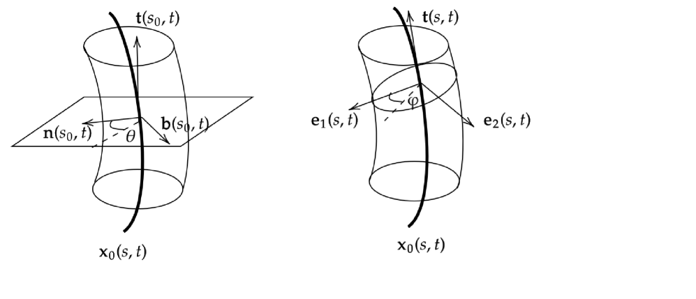
and, finally iii) one can use the so-called parallel or natural frame (see
figure 1
𝐱 = 𝐱 0 ( s 0 , t ) + x 1 𝐞 1 ( s 0 , t ) + x 2 𝐞 2 ( s 0 , t ) , 𝐱 subscript 𝐱 0 subscript 𝑠 0 𝑡 subscript 𝑥 1 subscript 𝐞 1 subscript 𝑠 0 𝑡 subscript 𝑥 2 subscript 𝐞 2 subscript 𝑠 0 𝑡 \mathbf{x}=\mathbf{x}_{0}(s_{0},t)+x_{1}\mathbf{e}_{1}(s_{0},t)+x_{2}\mathbf{e}_{2}(s_{0},t), (18)
where { 𝐞 1 ( s , t ) , 𝐞 2 ( s , t ) } subscript 𝐞 1 𝑠 𝑡 subscript 𝐞 2 𝑠 𝑡 \left\{\mathbf{e}_{1}(s,t),\mathbf{e}_{2}(s,t)\right\} 11 12 𝐱 𝐱 \mathbf{x} R 𝑅 R ( x n , x b , s ) subscript 𝑥 𝑛 subscript 𝑥 𝑏 𝑠 (x_{n},x_{b},s) ( r , θ , s ) 𝑟 𝜃 𝑠 (r,\theta,s) ( x 1 , x 2 , s ) subscript 𝑥 1 subscript 𝑥 2 𝑠 (x_{1},x_{2},s)
Figure 1: Sketch of the local Frenet-Serret frame (left) and the filament
parallel (or natural) frame (right).
Inside a tube of radius R 𝑅 R 𝐉 𝐉 \mathbf{J}
𝐉 = A 1 ( s , r , θ ) 𝐭 ( s ) + A 2 ( s , r , θ ) 𝐧 ( s ) + A 3 ( s , r , θ ) 𝐛 ( s ) , 𝐉 subscript 𝐴 1 𝑠 𝑟 𝜃 𝐭 𝑠 subscript 𝐴 2 𝑠 𝑟 𝜃 𝐧 𝑠 subscript 𝐴 3 𝑠 𝑟 𝜃 𝐛 𝑠 \mathbf{J}=A_{1}(s,r,\theta)\mathbf{t}(s)+A_{2}(s,r,\theta)\mathbf{n}(s)+A_{3}(s,r,\theta)\mathbf{b}(s),
and extend it to ℝ 3 superscript ℝ 3 \mathbb{R}^{3} η R ( d i s t ( 𝐱 , 𝐱 0 ( s , t ) ) \eta_{R}(dist(\mathbf{x},\mathbf{x}_{0}(s,t))
η R ( d i s t ( 𝐱 , 𝐱 0 ( s , t ) ) \displaystyle\eta_{R}(dist(\mathbf{x},\mathbf{x}_{0}(s,t)) ∈ \displaystyle\in C ∞ , superscript 𝐶 \displaystyle C^{\infty}, (19)
η R ( d i s t ( 𝐱 , 𝐱 0 ( s ) ) \displaystyle\eta_{R}(dist(\mathbf{x},\mathbf{x}_{0}(s)) = \displaystyle= 0 outside the tube of
radius R , 0 outside the tube of
radius 𝑅 \displaystyle 0\text{ outside the tube of
radius }R, (20)
η R ( d i s t ( 𝐱 , 𝐱 0 ( s ) ) \displaystyle\eta_{R}(dist(\mathbf{x},\mathbf{x}_{0}(s)) = \displaystyle= 1 inside the tube of
radius R / 2 . 1 inside the tube of
radius 𝑅 2 \displaystyle 1\text{ inside the tube of
radius }R/2. (21)
The vector field
𝐉 η = η R ( d i s t ( 𝐱 , 𝐱 0 ( s ) ) ) 𝐉 , subscript 𝐉 𝜂 subscript 𝜂 𝑅 𝑑 𝑖 𝑠 𝑡 𝐱 subscript 𝐱 0 𝑠 𝐉 \mathbf{J}_{\eta}=\eta_{R}(dist(\mathbf{x},\mathbf{x}_{0}(s)))\mathbf{J},
is identical to 𝐉 𝐉 \mathbf{J} R / 2 𝑅 2 R/2 ℝ 3 superscript ℝ 3 \mathbb{R}^{3} 𝐉 𝐉 \mathbf{J}
We can also define moving tubes around a filament 𝐱 0 ( s , t ) subscript 𝐱 0 𝑠 𝑡 \mathbf{x}_{0}(s,t) t ∈ [ 0 , T ] 𝑡 0 𝑇 t\in\left[0,T\right] R 𝑅 R
R < 1 2 max s , t | κ ( s , t ) | , 𝑅 1 2 subscript 𝑠 𝑡
𝜅 𝑠 𝑡 R<\frac{1}{2\max_{s,t}\left|\kappa(s,t)\right|},
and the corresponding moving cutoff function η R ( d i s t ( 𝐱 , 𝐱 0 ( s , t ) ) ) subscript 𝜂 𝑅 𝑑 𝑖 𝑠 𝑡 𝐱 subscript 𝐱 0 𝑠 𝑡 \eta_{R}(dist(\mathbf{x},\mathbf{x}_{0}(s,t)))
3 The Frenet-Serret frame and the parallel frame
Navier-Stokes equations are not invariant under coordinate changes such as
those described in the previous section (the Frenet-Serret frame and the
parallel frame coordinates). The fact that reference frames do translate and
rotate in a nonuniform way lead to the appearance of the so-called
”fictitious forces” in the new reference frame such as Coriolis and
centrifugal forces. Nevertheless, for a vortex filament, we will see in
section 6 t 𝑡 t ( 𝐧 , 𝐛 , 𝐭 ) 𝐧 𝐛 𝐭 (\mathbf{n},\mathbf{b},\mathbf{t}) ( 𝐞 1 , 𝐞 2 ) subscript 𝐞 1 subscript 𝐞 2 (\mathbf{e}_{1},\mathbf{e}_{2})
In order to understand how these fictitious forces appear, let us consider
first a local (in s 0 subscript 𝑠 0 s_{0} 1 x ′ = ( x n , x b , z ) superscript 𝑥 ′ subscript 𝑥 𝑛 subscript 𝑥 𝑏 𝑧 x^{\prime}=(x_{n},x_{b},z)
𝐱 = 𝐱 0 ( s 0 , t ) + x n 𝐧 ( s 0 , t ) + x b 𝐛 ( s 0 , t ) + z 𝐭 ( s 0 , t ) . 𝐱 subscript 𝐱 0 subscript 𝑠 0 𝑡 subscript 𝑥 𝑛 𝐧 subscript 𝑠 0 𝑡 subscript 𝑥 𝑏 𝐛 subscript 𝑠 0 𝑡 𝑧 𝐭 subscript 𝑠 0 𝑡 \mathbf{x}=\mathbf{x}_{0}(s_{0},t)+x_{n}\mathbf{n}(s_{0},t)+x_{b}\mathbf{b}(s_{0},t)+z\mathbf{t}(s_{0},t). (22)
If we consider now a trajectory 𝐱 ( t ) 𝐱 𝑡 \mathbf{x}(t) 𝐯 ( 𝐱 , t ) 𝐯 𝐱 𝑡 \mathbf{v}(\mathbf{x},t)
𝐯 ( 𝐱 ( t ) , t ) 𝐯 𝐱 𝑡 𝑡 \displaystyle\mathbf{v}(\mathbf{x}(t),t) = \displaystyle= d 𝐱 ( t ) d t 𝑑 𝐱 𝑡 𝑑 𝑡 \displaystyle\frac{d\mathbf{x}(t)}{dt} (23)
= \displaystyle= d 𝐱 0 ( s 0 , t ) d t + d x n ( t ) d t 𝐧 ( s 0 , t ) + d x b ( t ) d t 𝐛 ( s 0 , t ) + d z ( t ) d t 𝐭 ( s 0 , t ) 𝑑 subscript 𝐱 0 subscript 𝑠 0 𝑡 𝑑 𝑡 𝑑 subscript 𝑥 𝑛 𝑡 𝑑 𝑡 𝐧 subscript 𝑠 0 𝑡 𝑑 subscript 𝑥 𝑏 𝑡 𝑑 𝑡 𝐛 subscript 𝑠 0 𝑡 𝑑 𝑧 𝑡 𝑑 𝑡 𝐭 subscript 𝑠 0 𝑡 \displaystyle\frac{d\mathbf{x}_{0}(s_{0},t)}{dt}+\frac{dx_{n}(t)}{dt}\mathbf{n}(s_{0},t)+\frac{dx_{b}(t)}{dt}\mathbf{b}(s_{0},t)+\frac{dz(t)}{dt}\mathbf{t}(s_{0},t)
+ x n ( t ) d 𝐧 ( s 0 , t ) d t + x b ( t ) d 𝐛 ( s 0 , t ) d t + z ( t ) d 𝐭 ( s 0 , t ) d t subscript 𝑥 𝑛 𝑡 𝑑 𝐧 subscript 𝑠 0 𝑡 𝑑 𝑡 subscript 𝑥 𝑏 𝑡 𝑑 𝐛 subscript 𝑠 0 𝑡 𝑑 𝑡 𝑧 𝑡 𝑑 𝐭 subscript 𝑠 0 𝑡 𝑑 𝑡 \displaystyle+x_{n}(t)\frac{d\mathbf{n}(s_{0},t)}{dt}+x_{b}(t)\frac{d\mathbf{b}(s_{0},t)}{dt}+z(t)\frac{d\mathbf{t}(s_{0},t)}{dt}
= \displaystyle= d 𝐱 0 ( s 0 , t ) d t + 𝐯 ′ ( 𝐱 ′ ( t ) , t ) + ϖ × 𝐱 ′ ( t ) , 𝑑 subscript 𝐱 0 subscript 𝑠 0 𝑡 𝑑 𝑡 superscript 𝐯 ′ superscript 𝐱 ′ 𝑡 𝑡 italic-ϖ superscript 𝐱 ′ 𝑡 \displaystyle\frac{d\mathbf{x}_{0}(s_{0},t)}{dt}+\mathbf{v}^{\prime}(\mathbf{x}^{\prime}(t),t)+\mathbf{\varpi}\times\mathbf{x}^{\prime}(t),
which relates the velocities 𝐯 ( 𝐱 , t ) 𝐯 𝐱 𝑡 \mathbf{v}(\mathbf{x},t) 𝐯 ′ ( 𝐱 ′ , t ) superscript 𝐯 ′ superscript 𝐱 ′ 𝑡 \mathbf{v}^{\prime}(\mathbf{x}^{\prime},t) ϖ italic-ϖ \mathbf{\varpi} d d t ( 𝐧 , 𝐛 , 𝐭 ) 𝑑 𝑑 𝑡 𝐧 𝐛 𝐭 \frac{d}{dt}(\mathbf{n},\mathbf{b},\mathbf{t}) 25 26 28 ( 𝐮 1 , 𝐮 2 , 𝐮 3 ) = ( 𝐧 , 𝐛 , 𝐭 ) subscript 𝐮 1 subscript 𝐮 2 subscript 𝐮 3 𝐧 𝐛 𝐭 (\mathbf{u}_{1},\mathbf{u}_{2},\mathbf{u}_{3})=(\mathbf{n},\mathbf{b},\mathbf{t})
d 𝝎 ( 𝐱 ( t ) , t ) d t 𝑑 𝝎 𝐱 𝑡 𝑡 𝑑 𝑡 \displaystyle\frac{d\bm{\omega}(\mathbf{x}(t),t)}{dt}
= \displaystyle= d 𝝎 ′ ( 𝐱 ′ ( t ) , t ) d t = ∂ ω i ∂ t 𝐮 i ( t ) + ω i d 𝐮 i ( t ) d t + d 𝐱 ′ ( t ) d t ⋅ ∇ ω ′ ( 𝐱 ′ ( t ) , t ) 𝑑 superscript 𝝎 ′ superscript 𝐱 ′ 𝑡 𝑡 𝑑 𝑡 subscript 𝜔 𝑖 𝑡 subscript 𝐮 𝑖 𝑡 subscript 𝜔 𝑖 𝑑 subscript 𝐮 𝑖 𝑡 𝑑 𝑡 ⋅ 𝑑 superscript 𝐱 ′ 𝑡 𝑑 𝑡 ∇ superscript 𝜔 ′ superscript 𝐱 ′ 𝑡 𝑡 \displaystyle\frac{d\bm{\omega}^{\prime}(\mathbf{x}^{\prime}(t),t)}{dt}=\frac{\partial\omega_{i}}{\partial t}\mathbf{u}_{i}(t)+\omega_{i}\frac{d\mathbf{u}_{i}(t)}{dt}+\frac{d\mathbf{x}^{\prime}(t)}{dt}\cdot\nabla\mathbf{\omega}^{\prime}(\mathbf{x}^{\prime}(t),t)
= \displaystyle= ∂ ω i ∂ t 𝐮 i ( t ) + ω i d 𝐮 i ( t ) d t + ( 𝐯 ′ ( 𝐱 ′ ( t ) , t ) ⋅ ∇ ω i ( 𝐱 ′ ( t ) , t ) ) 𝐮 i ( t ) subscript 𝜔 𝑖 𝑡 subscript 𝐮 𝑖 𝑡 subscript 𝜔 𝑖 𝑑 subscript 𝐮 𝑖 𝑡 𝑑 𝑡 ⋅ superscript 𝐯 ′ superscript 𝐱 ′ 𝑡 𝑡 ∇ subscript 𝜔 𝑖 superscript 𝐱 ′ 𝑡 𝑡 subscript 𝐮 𝑖 𝑡 \displaystyle\frac{\partial\omega_{i}}{\partial t}\mathbf{u}_{i}(t)+\omega_{i}\frac{d\mathbf{u}_{i}(t)}{dt}+\left(\mathbf{v}^{\prime}(\mathbf{x}^{\prime}(t),t)\cdot\nabla\omega_{i}(\mathbf{x}^{\prime}(t),t)\right)\mathbf{u}_{i}(t)
+ x i ( t ) d 𝐮 i ( t ) d t ⋅ ∇ 𝝎 ′ ( 𝐱 ′ ( t ) , t ) ⋅ subscript 𝑥 𝑖 𝑡 𝑑 subscript 𝐮 𝑖 𝑡 𝑑 𝑡 ∇ superscript 𝝎 ′ superscript 𝐱 ′ 𝑡 𝑡 \displaystyle+x_{i}(t)\frac{d\mathbf{u}_{i}(t)}{dt}\cdot\nabla\bm{\omega}^{\prime}(\mathbf{x}^{\prime}(t),t)
= \displaystyle= ( ∂ ω i ∂ t + 𝐯 ′ ( 𝐱 ′ ( t ) , t ) ⋅ ∇ ω i ( 𝐱 ′ ( t ) , t ) ) 𝐮 i ( t ) + ϖ × 𝝎 ′ ( 𝐱 ′ ( t ) , t ) subscript 𝜔 𝑖 𝑡 ⋅ superscript 𝐯 ′ superscript 𝐱 ′ 𝑡 𝑡 ∇ subscript 𝜔 𝑖 superscript 𝐱 ′ 𝑡 𝑡 subscript 𝐮 𝑖 𝑡 italic-ϖ superscript 𝝎 ′ superscript 𝐱 ′ 𝑡 𝑡 \displaystyle\left(\frac{\partial\omega_{i}}{\partial t}+\mathbf{v}^{\prime}(\mathbf{x}^{\prime}(t),t)\cdot\nabla\omega_{i}(\mathbf{x}^{\prime}(t),t)\right)\mathbf{u}_{i}(t)+\mathbf{\varpi}\times\bm{\omega}^{\prime}(\mathbf{x}^{\prime}(t),t)
+ ( ϖ × 𝐱 ′ ( t ) ) ⋅ ∇ 𝝎 ′ ( 𝐱 ′ ( t ) , t ) , ⋅ italic-ϖ superscript 𝐱 ′ 𝑡 ∇ superscript 𝝎 ′ superscript 𝐱 ′ 𝑡 𝑡 \displaystyle+\left(\mathbf{\varpi}\times\mathbf{x}^{\prime}(t)\right)\cdot\nabla\bm{\omega}^{\prime}(\mathbf{x}^{\prime}(t),t),
where the first term at the right hand side is the convective derivative in
the Frenet-Serret coordinate frame and the last two terms are corrections
that amount to ”fictitious forces” for an observer in the moving frame. The
same can be said of the vortex stretching term:
𝝎 ( 𝐱 , t ) ⋅ ∇ 𝐯 ( 𝐱 , t ) = ω ′ ( 𝐱 ′ , t ) ⋅ ∇ 𝐯 ′ ( 𝐱 ′ , t ) + 𝝎 ′ ( 𝐱 ′ , t ) ⋅ ∇ ( ϖ × 𝐱 ′ ) , ⋅ 𝝎 𝐱 𝑡 ∇ 𝐯 𝐱 𝑡 ⋅ superscript 𝜔 ′ superscript 𝐱 ′ 𝑡 ∇ superscript 𝐯 ′ superscript 𝐱 ′ 𝑡 ⋅ superscript 𝝎 ′ superscript 𝐱 ′ 𝑡 ∇ italic-ϖ superscript 𝐱 ′ \bm{\omega}(\mathbf{x},t)\cdot\nabla\mathbf{v}(\mathbf{x},t)=\mathbf{\omega}^{\prime}(\mathbf{x}^{\prime},t)\cdot\nabla\mathbf{v}^{\prime}(\mathbf{x}^{\prime},t)+\bm{\omega}^{\prime}(\mathbf{x}^{\prime},t)\cdot\nabla\left(\mathbf{\varpi}\times\mathbf{x}^{\prime}\right),
with an extra term at the right hand side while the viscous term remains
unchanged under the coordinate change since the Laplacian operator is
invariant under translations and rotations.
We compute and estimate next the vector ϖ italic-ϖ \mathbf{\varpi}
d 𝐱 d t = − κ Γ 4 π ( log ( ν t ) 1 2 ) 𝐛 , \frac{d\mathbf{x}}{dt}=-\frac{\kappa\Gamma}{4\pi}\left(\log(\nu t)^{\frac{1}{2}}\right)\mathbf{b},
we introduce
t ′ = Γ 4 π ∫ 0 t log ( ν τ ) 1 2 d τ , t^{\prime}=\frac{\Gamma}{4\pi}\int_{0}^{t}\log(\nu\tau)^{\frac{1}{2}}d\tau,
and compute
d 𝐭 d t ′ 𝑑 𝐭 𝑑 superscript 𝑡 ′ \displaystyle\frac{d\mathbf{t}}{dt^{\prime}} = \displaystyle= κ s 𝐛 + κ 𝐛 s = κ s 𝐛 − κ τ 𝐧 = − κ s 𝐧 × 𝐭 − κ τ 𝐛 × 𝐭 , subscript 𝜅 𝑠 𝐛 𝜅 subscript 𝐛 𝑠 subscript 𝜅 𝑠 𝐛 𝜅 𝜏 𝐧 subscript 𝜅 𝑠 𝐧 𝐭 𝜅 𝜏 𝐛 𝐭 \displaystyle\kappa_{s}\mathbf{b}+\kappa\mathbf{b}_{s}=\kappa_{s}\mathbf{b}-\kappa\tau\mathbf{n=-}\kappa_{s}\mathbf{n}\times\mathbf{t-}\kappa\tau\mathbf{b}\times\mathbf{t},
d ( κ 𝐧 ) d t ′ 𝑑 𝜅 𝐧 𝑑 superscript 𝑡 ′ \displaystyle\frac{d(\kappa\mathbf{n})}{dt^{\prime}} = \displaystyle= κ s s 𝐛 + κ s 𝐛 s − ( κ τ ) s 𝐧 − κ τ ( − κ 𝐭 + τ 𝐛 ) , subscript 𝜅 𝑠 𝑠 𝐛 subscript 𝜅 𝑠 subscript 𝐛 𝑠 subscript 𝜅 𝜏 𝑠 𝐧 𝜅 𝜏 𝜅 𝐭 𝜏 𝐛 \displaystyle\kappa_{ss}\mathbf{b}+\kappa_{s}\mathbf{b}_{s}-(\kappa\tau)_{s}\mathbf{n}-\kappa\tau\left(-\kappa\mathbf{t}+\tau\mathbf{b}\right),
so that
d 𝐧 d t ′ = − κ t ′ + κ s τ + ( κ τ ) s κ 𝐧 + κ τ 𝐭 + κ s s − κ τ 2 κ 𝐛 . 𝑑 𝐧 𝑑 superscript 𝑡 ′ subscript 𝜅 superscript 𝑡 ′ subscript 𝜅 𝑠 𝜏 subscript 𝜅 𝜏 𝑠 𝜅 𝐧 𝜅 𝜏 𝐭 subscript 𝜅 𝑠 𝑠 𝜅 superscript 𝜏 2 𝜅 𝐛 \frac{d\mathbf{n}}{dt^{\prime}}=-\frac{\kappa_{t^{\prime}}+\kappa_{s}\tau+(\kappa\tau)_{s}}{\kappa}\mathbf{n+}\kappa\tau\mathbf{t}+\frac{\kappa_{ss}-\kappa\tau^{2}}{\kappa}\mathbf{b}.
Since
0 = 𝐧 ⋅ d 𝐧 d t ′ = − κ t ′ + κ s τ + ( κ τ ) s κ , 0 ⋅ 𝐧 𝑑 𝐧 𝑑 superscript 𝑡 ′ subscript 𝜅 superscript 𝑡 ′ subscript 𝜅 𝑠 𝜏 subscript 𝜅 𝜏 𝑠 𝜅 0=\mathbf{n}\cdot\frac{d\mathbf{n}}{dt^{\prime}}=-\frac{\kappa_{t^{\prime}}+\kappa_{s}\tau+(\kappa\tau)_{s}}{\kappa},
we have
d 𝐧 d t ′ 𝑑 𝐧 𝑑 superscript 𝑡 ′ \displaystyle\frac{d\mathbf{n}}{dt^{\prime}} = \displaystyle= κ τ 𝐭 + κ s s − κ τ 2 κ 𝐛 𝜅 𝜏 𝐭 subscript 𝜅 𝑠 𝑠 𝜅 superscript 𝜏 2 𝜅 𝐛 \displaystyle\kappa\tau\mathbf{t}+\frac{\kappa_{ss}-\kappa\tau^{2}}{\kappa}\mathbf{b}
= \displaystyle= κ s s − κ τ 2 κ 𝐭 × 𝐧 − κ τ 𝐛 × 𝐧 . subscript 𝜅 𝑠 𝑠 𝜅 superscript 𝜏 2 𝜅 𝐭 𝐧 𝜅 𝜏 𝐛 𝐧 \displaystyle\frac{\kappa_{ss}-\kappa\tau^{2}}{\kappa}\mathbf{t}\times\mathbf{n-}\kappa\tau\mathbf{b}\times\mathbf{n}.
Notice that, by equation (8
κ s s − κ τ 2 κ = ∫ τ t ′ 𝑑 s − 1 2 κ 2 , subscript 𝜅 𝑠 𝑠 𝜅 superscript 𝜏 2 𝜅 subscript 𝜏 superscript 𝑡 ′ differential-d 𝑠 1 2 superscript 𝜅 2 \frac{\kappa_{ss}-\kappa\tau^{2}}{\kappa}=\int\tau_{t^{\prime}}ds-\frac{1}{2}\kappa^{2}, (24)
which is bounded.
Note now
d 𝐛 d t ′ 𝑑 𝐛 𝑑 superscript 𝑡 ′ \displaystyle\frac{d\mathbf{b}}{dt^{\prime}} = \displaystyle= 𝐭 × d 𝐧 d t ′ + d 𝐭 d t ′ × 𝐧 = κ s s − κ τ 2 κ 𝐭 × 𝐛 + κ s 𝐛 × 𝐧 𝐭 𝑑 𝐧 𝑑 superscript 𝑡 ′ 𝑑 𝐭 𝑑 superscript 𝑡 ′ 𝐧 subscript 𝜅 𝑠 𝑠 𝜅 superscript 𝜏 2 𝜅 𝐭 𝐛 subscript 𝜅 𝑠 𝐛 𝐧 \displaystyle\mathbf{t}\times\frac{d\mathbf{n}}{dt^{\prime}}+\frac{d\mathbf{t}}{dt^{\prime}}\times\mathbf{n}=\frac{\kappa_{ss}-\kappa\tau^{2}}{\kappa}\mathbf{t}\times\mathbf{b}+\kappa_{s}\mathbf{b}\times\mathbf{n}
= \displaystyle= κ s s − κ τ 2 κ 𝐭 × 𝐛 − κ s 𝐧 × 𝐛 . subscript 𝜅 𝑠 𝑠 𝜅 superscript 𝜏 2 𝜅 𝐭 𝐛 subscript 𝜅 𝑠 𝐧 𝐛 \displaystyle\frac{\kappa_{ss}-\kappa\tau^{2}}{\kappa}\mathbf{t}\times\mathbf{b}-\kappa_{s}\mathbf{n}\times\mathbf{b}.
Hence, by introducing
ϖ = Γ 2 π log ( ν t ) [ κ s s − κ τ 2 κ 𝐭 − κ s 𝐧 − κ τ 𝐛 ] , bold-italic-ϖ Γ 2 𝜋 𝜈 𝑡 delimited-[] subscript 𝜅 𝑠 𝑠 𝜅 superscript 𝜏 2 𝜅 𝐭 subscript 𝜅 𝑠 𝐧 𝜅 𝜏 𝐛 \bm{\varpi}=\frac{\Gamma}{2\pi}\log(\nu t)\left[\frac{\kappa_{ss}-\kappa\tau^{2}}{\kappa}\mathbf{t}-\kappa_{s}\mathbf{\mathbf{n}-}\kappa\tau\mathbf{b}\right], (25)
we have
d 𝐭 d t 𝑑 𝐭 𝑑 𝑡 \displaystyle\frac{d\mathbf{t}}{dt} = \displaystyle= ϖ × 𝐭 , bold-italic-ϖ 𝐭 \displaystyle\bm{\varpi}\times\mathbf{t}, (26)
d 𝐧 d t 𝑑 𝐧 𝑑 𝑡 \displaystyle\frac{d\mathbf{n}}{dt} = \displaystyle= ϖ × 𝐧 , bold-italic-ϖ 𝐧 \displaystyle\bm{\varpi}\times\mathbf{n}, (27)
d 𝐛 d t 𝑑 𝐛 𝑑 𝑡 \displaystyle\frac{d\mathbf{b}}{dt} = \displaystyle= ϖ × 𝐛 , bold-italic-ϖ 𝐛 \displaystyle\bm{\varpi}\times\mathbf{b}, (28)
where ϖ bold-italic-ϖ \bm{\varpi} 26 28 ϖ bold-italic-ϖ \bm{\varpi} 25
| ϖ | ≤ C Γ | log ( ν t ) | . bold-italic-ϖ 𝐶 Γ 𝜈 𝑡 \left|\bm{\varpi}\right|\leq C\Gamma\left|\log(\nu t)\right|.
In the case of the parallel (or natural) frame coordinates ( x 1 , x 2 , s ) subscript 𝑥 1 subscript 𝑥 2 𝑠 (x_{1},x_{2},s) 1 18 ( 𝐞 1 ( s , t ) , 𝐞 2 ( s , t ) ) subscript 𝐞 1 𝑠 𝑡 subscript 𝐞 2 𝑠 𝑡 (\mathbf{e}_{1}(s,t),\mathbf{e}_{2}(s,t)) x 0 ( s , t ) subscript 𝑥 0 𝑠 𝑡 x_{0}(s,t)
𝐧 ( s , t ) 𝐧 𝑠 𝑡 \displaystyle\mathbf{n}(s,t) = \displaystyle= cos ( θ 0 ( s , t ) ) 𝐞 1 ( s , t ) + sin ( θ 0 ( s , t ) ) 𝐞 2 ( s , t ) , subscript 𝜃 0 𝑠 𝑡 subscript 𝐞 1 𝑠 𝑡 subscript 𝜃 0 𝑠 𝑡 subscript 𝐞 2 𝑠 𝑡 \displaystyle\cos\left(\theta_{0}(s,t)\right)\mathbf{e}_{1}(s,t)+\sin\left(\theta_{0}(s,t)\right)\mathbf{e}_{2}(s,t), (29)
𝐛 ( s , t ) 𝐛 𝑠 𝑡 \displaystyle\mathbf{b}(s,t) = \displaystyle= − sin ( θ 0 ( s , t ) ) 𝐞 1 ( s , t ) + cos ( θ 0 ( s , t ) ) 𝐞 2 ( s , t ) , subscript 𝜃 0 𝑠 𝑡 subscript 𝐞 1 𝑠 𝑡 subscript 𝜃 0 𝑠 𝑡 subscript 𝐞 2 𝑠 𝑡 \displaystyle-\sin\left(\theta_{0}(s,t)\right)\mathbf{e}_{1}(s,t)+\cos\left(\theta_{0}(s,t)\right)\mathbf{e}_{2}(s,t), (30)
where
θ 0 ( s , t ) = ∫ s 0 s τ ( s ′ , t ) 𝑑 s ′ , subscript 𝜃 0 𝑠 𝑡 superscript subscript subscript 𝑠 0 𝑠 𝜏 superscript 𝑠 ′ 𝑡 differential-d superscript 𝑠 ′ \theta_{0}(s,t)=\int_{s_{0}}^{s}\tau(s^{\prime},t)ds^{\prime},
and s 0 subscript 𝑠 0 s_{0} ( x 1 , x 2 ) subscript 𝑥 1 subscript 𝑥 2 (x_{1},x_{2})
x 1 subscript 𝑥 1 \displaystyle x_{1} = \displaystyle= r cos φ , 𝑟 𝜑 \displaystyle r\cos\varphi,
x 2 subscript 𝑥 2 \displaystyle x_{2} = \displaystyle= r sin φ . 𝑟 𝜑 \displaystyle r\sin\varphi.
Hence, one can rewrite
x n subscript 𝑥 𝑛 \displaystyle x_{n} = \displaystyle= r cos ( φ − θ 0 ( s , t ) ) , 𝑟 𝜑 subscript 𝜃 0 𝑠 𝑡 \displaystyle r\cos\left(\varphi-\theta_{0}(s,t)\right),
x b subscript 𝑥 𝑏 \displaystyle x_{b} = \displaystyle= r sin ( φ − θ 0 ( s , t ) ) . 𝑟 𝜑 subscript 𝜃 0 𝑠 𝑡 \displaystyle r\sin\left(\varphi-\theta_{0}(s,t)\right).
In this way, the system ( r , φ , s ) 𝑟 𝜑 𝑠 (r,\varphi,s)
( 𝐞 r , 𝐞 φ , 𝐞 s ) = ( cos φ 𝐞 1 + sin φ 𝐞 2 , − sin φ 𝐞 1 + cos φ 𝐞 2 , 𝐭 ) , subscript 𝐞 𝑟 subscript 𝐞 𝜑 subscript 𝐞 𝑠 𝜑 subscript 𝐞 1 𝜑 subscript 𝐞 2 𝜑 subscript 𝐞 1 𝜑 subscript 𝐞 2 𝐭 (\mathbf{e}_{r},\mathbf{e}_{\varphi},\mathbf{e}_{s})=(\cos\varphi\mathbf{e}_{1}+\sin\varphi\mathbf{e}_{2},-\sin\varphi\mathbf{e}_{1}+\cos\varphi\mathbf{e}_{2},\mathbf{t}), (31)
once we have untwisted the origin of the angular coordinate according to the
torsion of 𝐱 0 ( s , t ) subscript 𝐱 0 𝑠 𝑡 \mathbf{x}_{0}(s,t)
h r = 1 , h φ = 1 , h s = 1 − κ r cos ( φ − θ 0 ( s , t ) ) , formulae-sequence subscript ℎ 𝑟 1 formulae-sequence subscript ℎ 𝜑 1 subscript ℎ 𝑠 1 𝜅 𝑟 𝜑 subscript 𝜃 0 𝑠 𝑡 h_{r}=1,h_{\varphi}=1,h_{s}=1-\kappa r\cos\left(\varphi-\theta_{0}(s,t)\right), (32)
and hence the volume element d V i 𝑑 subscript 𝑉 𝑖 dV_{i} d V f s 𝑑 subscript 𝑉 𝑓 𝑠 dV_{fs}
d V f s = ( 1 − κ r cos ( φ − θ 0 ( s , t ) ) ) d V i . 𝑑 subscript 𝑉 𝑓 𝑠 1 𝜅 𝑟 𝜑 subscript 𝜃 0 𝑠 𝑡 𝑑 subscript 𝑉 𝑖 dV_{fs}=\left(1-\kappa r\cos\left(\varphi-\theta_{0}(s,t)\right)\right)dV_{i}. (33)
Analogously to (23 𝐯 ( 𝐱 , t ) 𝐯 𝐱 𝑡 \mathbf{v}(\mathbf{x},t) 𝐯 ~ ( 𝐱 ~ , t ) ~ 𝐯 ~ 𝐱 𝑡 \widetilde{\mathbf{v}}(\widetilde{\mathbf{x}},t)
𝐯 ( 𝐱 ( t ) , t ) 𝐯 𝐱 𝑡 𝑡 \displaystyle\mathbf{v}(\mathbf{x}(t),t) (34)
= \displaystyle= 𝐱 0 , t ( s ( t ) , t ) + s ′ ( t ) 𝐭 ( s ( t ) , t ) + x 1 , t ( t ) 𝐞 1 ( s ( t ) , t ) + x 2 , t ( t ) 𝐞 2 ( s ( t ) , t ) subscript 𝐱 0 𝑡
𝑠 𝑡 𝑡 superscript 𝑠 ′ 𝑡 𝐭 𝑠 𝑡 𝑡 subscript 𝑥 1 𝑡
𝑡 subscript 𝐞 1 𝑠 𝑡 𝑡 subscript 𝑥 2 𝑡
𝑡 subscript 𝐞 2 𝑠 𝑡 𝑡 \displaystyle\mathbf{x}_{0,t}(s(t),t)+s^{\prime}(t)\mathbf{t}(s(t),t)+x_{1,t}(t)\mathbf{e}_{1}(s(t),t)+x_{2,t}(t)\mathbf{e}_{2}(s(t),t)
+ x 1 ( t ) ( 𝐞 1 , t ( s ( t ) , t ) + s ′ ( t ) 𝐞 1 , s ( s ( t ) , t ) ) + x 2 ( t ) ( 𝐞 2 , t ( s ( t ) , t ) + s ′ ( t ) 𝐞 2 , s ( s ( t ) , t ) ) subscript 𝑥 1 𝑡 subscript 𝐞 1 𝑡
𝑠 𝑡 𝑡 superscript 𝑠 ′ 𝑡 subscript 𝐞 1 𝑠
𝑠 𝑡 𝑡 subscript 𝑥 2 𝑡 subscript 𝐞 2 𝑡
𝑠 𝑡 𝑡 superscript 𝑠 ′ 𝑡 subscript 𝐞 2 𝑠
𝑠 𝑡 𝑡 \displaystyle+x_{1}(t)\left(\mathbf{e}_{1,t}(s(t),t)+s^{\prime}(t)\mathbf{e}_{1,s}(s(t),t)\right)+x_{2}(t)\left(\mathbf{e}_{2,t}(s(t),t)+s^{\prime}(t)\mathbf{e}_{2,s}(s(t),t)\right)
= \displaystyle= 𝐱 0 , t ( s ( t ) , t ) + v s ( t ) 𝐭 ( s ( t ) , t ) + v 1 ( t ) 𝐞 1 ( s ( t ) , t ) + v 2 ( t ) 𝐞 2 ( s ( t ) , t ) subscript 𝐱 0 𝑡
𝑠 𝑡 𝑡 subscript 𝑣 𝑠 𝑡 𝐭 𝑠 𝑡 𝑡 subscript 𝑣 1 𝑡 subscript 𝐞 1 𝑠 𝑡 𝑡 subscript 𝑣 2 𝑡 subscript 𝐞 2 𝑠 𝑡 𝑡 \displaystyle\mathbf{x}_{0,t}(s(t),t)+v_{s}(t)\mathbf{t}(s(t),t)+v_{1}(t)\mathbf{e}_{1}(s(t),t)+v_{2}(t)\mathbf{e}_{2}(s(t),t)
+ x 1 ( t ) ( 𝐞 1 , t ( s ( t ) , t ) + v s ( t ) 𝐞 1 , s ( s ( t ) , t ) ) + x 2 ( t ) ( 𝐞 2 , t ( s ( t ) , t ) + v s ( t ) 𝐞 2 , s ( s ( t ) , t ) ) subscript 𝑥 1 𝑡 subscript 𝐞 1 𝑡
𝑠 𝑡 𝑡 subscript 𝑣 𝑠 𝑡 subscript 𝐞 1 𝑠
𝑠 𝑡 𝑡 subscript 𝑥 2 𝑡 subscript 𝐞 2 𝑡
𝑠 𝑡 𝑡 subscript 𝑣 𝑠 𝑡 subscript 𝐞 2 𝑠
𝑠 𝑡 𝑡 \displaystyle+x_{1}(t)\left(\mathbf{e}_{1,t}(s(t),t)+v_{s}(t)\mathbf{e}_{1,s}(s(t),t)\right)+x_{2}(t)\left(\mathbf{e}_{2,t}(s(t),t)+v_{s}(t)\mathbf{e}_{2,s}(s(t),t)\right)
= \displaystyle= d 𝐱 0 ( s , t ) d t + 𝐯 ~ ( 𝐱 ~ ( t ) , t ) + x 1 ( t ) ( 𝐞 1 , t ( s ( t ) , t ) + v s ( t ) 𝐞 1 , s ( s ( t ) , t ) ) 𝑑 subscript 𝐱 0 𝑠 𝑡 𝑑 𝑡 ~ 𝐯 ~ 𝐱 𝑡 𝑡 subscript 𝑥 1 𝑡 subscript 𝐞 1 𝑡
𝑠 𝑡 𝑡 subscript 𝑣 𝑠 𝑡 subscript 𝐞 1 𝑠
𝑠 𝑡 𝑡 \displaystyle\frac{d\mathbf{x}_{0}(s,t)}{dt}+\widetilde{\mathbf{v}}(\widetilde{\mathbf{x}}(t),t)+x_{1}(t)\left(\mathbf{e}_{1,t}(s(t),t)+v_{s}(t)\mathbf{e}_{1,s}(s(t),t)\right)
+ x 2 ( t ) ( 𝐞 2 , t ( s ( t ) , t ) + v s ( t ) 𝐞 2 , s ( s ( t ) , t ) ) , subscript 𝑥 2 𝑡 subscript 𝐞 2 𝑡
𝑠 𝑡 𝑡 subscript 𝑣 𝑠 𝑡 subscript 𝐞 2 𝑠
𝑠 𝑡 𝑡 \displaystyle+x_{2}(t)\left(\mathbf{e}_{2,t}(s(t),t)+v_{s}(t)\mathbf{e}_{2,s}(s(t),t)\right),
where we note the appearance of time and s 𝑠 s 𝐞 1 ( s , t ) subscript 𝐞 1 𝑠 𝑡 \mathbf{e}_{1}(s,t) 𝐞 2 ( s , t ) subscript 𝐞 2 𝑠 𝑡 \mathbf{e}_{2}(s,t) v s subscript 𝑣 𝑠 v_{s} 𝐯 ( 𝐱 , t ) 𝐯 𝐱 𝑡 \mathbf{v}(\mathbf{x},t) 𝐱 0 ( s , t ) subscript 𝐱 0 𝑠 𝑡 \mathbf{x}_{0}(s,t) 6 78 79 ( 𝐞 1 ( s , t ) , 𝐞 2 ( s , t ) ) subscript 𝐞 1 𝑠 𝑡 subscript 𝐞 2 𝑠 𝑡 (\mathbf{e}_{1}(s,t),\mathbf{e}_{2}(s,t))
Lemma 4 .
Given a vortex filament 𝐱 0 ( s , t ) subscript 𝐱 0 𝑠 𝑡 \mathbf{x}_{0}(s,t) ∈ C ( ( 0 . T ) , C 2 ( T 1 , S 2 ) ) \in C((0.T),C^{2}(T^{1},S^{2})) ( 𝐞 1 ( s , t ) , 𝐞 2 ( s , t ) ) subscript 𝐞 1 𝑠 𝑡 subscript 𝐞 2 𝑠 𝑡 (\mathbf{e}_{1}(s,t),\mathbf{e}_{2}(s,t))
| 𝐞 1 , s ( s , t ) | + | 𝐞 2 , s ( s , t ) | subscript 𝐞 1 𝑠
𝑠 𝑡 subscript 𝐞 2 𝑠
𝑠 𝑡 \displaystyle\left|\mathbf{e}_{1,s}(s,t)\right|+\left|\mathbf{e}_{2,s}(s,t)\right| ≤ \displaystyle\leq C 𝐶 \displaystyle C
| 𝐞 1 , t ( s , t ) | + | 𝐞 2 , t ( s , t ) | subscript 𝐞 1 𝑡
𝑠 𝑡 subscript 𝐞 2 𝑡
𝑠 𝑡 \displaystyle\left|\mathbf{e}_{1,t}(s,t)\right|+\left|\mathbf{e}_{2,t}(s,t)\right| ≤ \displaystyle\leq C Γ | log ( ν t ) | 𝐶 Γ 𝜈 𝑡 \displaystyle C\Gamma\left|\log(\nu t)\right|
Proof. The estimate for 𝐞 i , s ( s , t ) subscript 𝐞 𝑖 𝑠
𝑠 𝑡 \mathbf{e}_{i,s}(s,t) 11 12 𝐭 s = κ 𝐧 subscript 𝐭 𝑠 𝜅 𝐧 \mathbf{t}_{s}=\kappa\mathbf{n} 𝐞 1 , t ( s , t ) subscript 𝐞 1 𝑡
𝑠 𝑡 \mathbf{e}_{1,t}(s,t) 29 30
𝐞 1 ( s , t ) subscript 𝐞 1 𝑠 𝑡 \displaystyle\mathbf{e}_{1}(s,t) = \displaystyle= cos ( θ 0 ( s , t ) ) 𝐧 ( s , t ) − sin ( θ 0 ( s , t ) ) 𝐛 ( s , t ) , subscript 𝜃 0 𝑠 𝑡 𝐧 𝑠 𝑡 subscript 𝜃 0 𝑠 𝑡 𝐛 𝑠 𝑡 \displaystyle\cos\left(\theta_{0}(s,t)\right)\mathbf{n}(s,t)-\sin\left(\theta_{0}(s,t)\right)\mathbf{b}(s,t),
𝐞 2 ( s , t ) subscript 𝐞 2 𝑠 𝑡 \displaystyle\mathbf{e}_{2}(s,t) = \displaystyle= sin ( θ 0 ( s , t ) ) 𝐧 ( s , t ) + cos ( θ 0 ( s , t ) ) 𝐛 ( s , t ) , subscript 𝜃 0 𝑠 𝑡 𝐧 𝑠 𝑡 subscript 𝜃 0 𝑠 𝑡 𝐛 𝑠 𝑡 \displaystyle\sin\left(\theta_{0}(s,t)\right)\mathbf{n}(s,t)+\cos\left(\theta_{0}(s,t)\right)\mathbf{b}(s,t),
and hence, for 𝐞 1 , t ( s , t ) subscript 𝐞 1 𝑡
𝑠 𝑡 \mathbf{e}_{1,t}(s,t)
𝐞 1 , t ( s , t ) subscript 𝐞 1 𝑡
𝑠 𝑡 \displaystyle\mathbf{e}_{1,t}(s,t) = \displaystyle= ( − sin ( θ 0 ( s , t ) ) 𝐧 ( s , t ) − cos ( θ 0 ( s , t ) ) 𝐛 ( s , t ) ) θ 0 , t ( s , t ) subscript 𝜃 0 𝑠 𝑡 𝐧 𝑠 𝑡 subscript 𝜃 0 𝑠 𝑡 𝐛 𝑠 𝑡 subscript 𝜃 0 𝑡
𝑠 𝑡 \displaystyle\left(-\sin\left(\theta_{0}(s,t)\right)\mathbf{n}(s,t)-\cos\left(\theta_{0}(s,t)\right)\mathbf{b}(s,t)\right)\theta_{0,t}(s,t)
+ cos ( θ 0 ( s , t ) ) 𝐧 t ( s , t ) − sin ( θ 0 ( s , t ) ) 𝐛 t ( s , t ) subscript 𝜃 0 𝑠 𝑡 subscript 𝐧 𝑡 𝑠 𝑡 subscript 𝜃 0 𝑠 𝑡 subscript 𝐛 𝑡 𝑠 𝑡 \displaystyle+\cos\left(\theta_{0}(s,t)\right)\mathbf{n}_{t}(s,t)-\sin\left(\theta_{0}(s,t)\right)\mathbf{b}_{t}(s,t)
= \displaystyle= ( − sin ( θ 0 ( s , t ) ) 𝐧 ( s , t ) − cos ( θ 0 ( s , t ) ) 𝐛 ( s , t ) ) ∫ s 0 s τ t ( s ′ , t ) 𝑑 s ′ subscript 𝜃 0 𝑠 𝑡 𝐧 𝑠 𝑡 subscript 𝜃 0 𝑠 𝑡 𝐛 𝑠 𝑡 superscript subscript subscript 𝑠 0 𝑠 subscript 𝜏 𝑡 superscript 𝑠 ′ 𝑡 differential-d superscript 𝑠 ′ \displaystyle\left(-\sin\left(\theta_{0}(s,t)\right)\mathbf{n}(s,t)-\cos\left(\theta_{0}(s,t)\right)\mathbf{b}(s,t)\right)\int_{s_{0}}^{s}\tau_{t}(s^{\prime},t)ds^{\prime}
+ cos ( θ 0 ( s , t ) ) ϖ × 𝐧 − sin ( θ 0 ( s , t ) ) ϖ × 𝐛 subscript 𝜃 0 𝑠 𝑡 bold-italic-ϖ 𝐧 subscript 𝜃 0 𝑠 𝑡 bold-italic-ϖ 𝐛 \displaystyle+\cos\left(\theta_{0}(s,t)\right)\bm{\varpi}\times\mathbf{n}-\sin\left(\theta_{0}(s,t)\right)\bm{\varpi}\times\mathbf{b}
= \displaystyle= ( − sin ( θ 0 ( s , t ) ) 𝐧 ( s , t ) − cos ( θ 0 ( s , t ) ) 𝐛 ( s , t ) ) ∫ s 0 s τ t ( s ′ , t ) 𝑑 s ′ subscript 𝜃 0 𝑠 𝑡 𝐧 𝑠 𝑡 subscript 𝜃 0 𝑠 𝑡 𝐛 𝑠 𝑡 superscript subscript subscript 𝑠 0 𝑠 subscript 𝜏 𝑡 superscript 𝑠 ′ 𝑡 differential-d superscript 𝑠 ′ \displaystyle\left(-\sin\left(\theta_{0}(s,t)\right)\mathbf{n}(s,t)-\cos\left(\theta_{0}(s,t)\right)\mathbf{b}(s,t)\right)\int_{s_{0}}^{s}\tau_{t}(s^{\prime},t)ds^{\prime}
+ cos ( θ 0 ( s , t ) ) ( ∫ τ t ′ 𝑑 s − 1 2 κ 2 ) 𝐛 + cos ( θ 0 ( s , t ) ) Γ 2 π log ( ν t ) κ τ 𝐭 subscript 𝜃 0 𝑠 𝑡 subscript 𝜏 superscript 𝑡 ′ differential-d 𝑠 1 2 superscript 𝜅 2 𝐛 subscript 𝜃 0 𝑠 𝑡 Γ 2 𝜋 𝜈 𝑡 𝜅 𝜏 𝐭 \displaystyle+\cos\left(\theta_{0}(s,t)\right)\left(\int\tau_{t^{\prime}}ds-\frac{1}{2}\kappa^{2}\right)\mathbf{b}+\cos\left(\theta_{0}(s,t)\right)\frac{\Gamma}{2\pi}\log(\nu t)\kappa\tau\mathbf{t}
+ sin ( θ 0 ( s , t ) ) ( ∫ τ t ′ 𝑑 s − 1 2 κ 2 ) 𝐧 + sin ( θ 0 ( s , t ) ) Γ 2 π log ( ν t ) κ s 𝐭 subscript 𝜃 0 𝑠 𝑡 subscript 𝜏 superscript 𝑡 ′ differential-d 𝑠 1 2 superscript 𝜅 2 𝐧 subscript 𝜃 0 𝑠 𝑡 Γ 2 𝜋 𝜈 𝑡 subscript 𝜅 𝑠 𝐭 \displaystyle+\sin\left(\theta_{0}(s,t)\right)\left(\int\tau_{t^{\prime}}ds-\frac{1}{2}\kappa^{2}\right)\mathbf{n}+\sin\left(\theta_{0}(s,t)\right)\frac{\Gamma}{2\pi}\log(\nu t)\kappa_{s}\mathbf{t}
= \displaystyle= − 1 2 κ 2 𝐞 2 ( s , t ) + Γ 2 π log ( ν t ) ( cos ( θ 0 ( s , t ) ) κ τ + sin ( θ 0 ( s , t ) ) κ s ) 𝐭 , 1 2 superscript 𝜅 2 subscript 𝐞 2 𝑠 𝑡 Γ 2 𝜋 𝜈 𝑡 subscript 𝜃 0 𝑠 𝑡 𝜅 𝜏 subscript 𝜃 0 𝑠 𝑡 subscript 𝜅 𝑠 𝐭 \displaystyle-\frac{1}{2}\kappa^{2}\mathbf{e}_{2}(s,t)+\frac{\Gamma}{2\pi}\log(\nu t)\left(\cos\left(\theta_{0}(s,t)\right)\kappa\tau+\sin\left(\theta_{0}(s,t)\right)\kappa_{s}\right)\mathbf{t},
and using (24 28
| 𝐞 1 , t ( s , t ) | ≤ C | log ( ν t ) | . subscript 𝐞 1 𝑡
𝑠 𝑡 𝐶 𝜈 𝑡 \left|\mathbf{e}_{1,t}(s,t)\right|\leq C\left|\log(\nu t)\right|.
The vector 𝐞 2 , t ( s , t ) subscript 𝐞 2 𝑡
𝑠 𝑡 \mathbf{e}_{2,t}(s,t)
We describe next the general strategy for our analysis in the next sections.
We write
𝝎 𝝎 \displaystyle\bm{\omega} = \displaystyle= 𝝎 0 + 𝝎 ~ , subscript 𝝎 0 ~ 𝝎 \displaystyle\bm{\omega}_{0}+\widetilde{\bm{\omega}},
𝐯 𝐯 \displaystyle\mathbf{v} = \displaystyle= 𝐯 0 + 𝐯 ~ , subscript 𝐯 0 ~ 𝐯 \displaystyle\mathbf{v}_{0}+\widetilde{\mathbf{v}},
where 𝝎 0 subscript 𝝎 0 \bm{\omega}_{0} 𝐯 0 subscript 𝐯 0 \mathbf{v}_{0} 𝝎 0 subscript 𝝎 0 \bm{\omega}_{0}
∂ 𝝎 0 ∂ t + 𝒗 0 ⋅ ∇ 𝐱 𝝎 0 − 𝝎 0 ⋅ ∇ 𝐱 𝐯 0 − ν Δ 𝐱 𝝎 0 = − 𝐅 ( 𝐱 , t ) , subscript 𝝎 0 𝑡 ⋅ subscript 𝒗 0 subscript ∇ 𝐱 subscript 𝝎 0 ⋅ subscript 𝝎 0 subscript ∇ 𝐱 subscript 𝐯 0 𝜈 subscript Δ 𝐱 subscript 𝝎 0 𝐅 𝐱 𝑡 \frac{\partial\bm{\omega}_{0}}{\partial t}+\bm{v}_{0}\cdot\nabla_{\mathbf{x}}\bm{\omega}_{0}-\bm{\omega}_{0}\cdot\nabla_{\mathbf{x}}\mathbf{v}_{0}-\nu\Delta_{\mathbf{x}}\bm{\omega}_{0}=-\mathbf{F}(\mathbf{x},t),
where 𝐅 ( 𝐱 , t ) 𝐅 𝐱 𝑡 \mathbf{F}(\mathbf{x},t) 𝝎 0 subscript 𝝎 0 \bm{\omega}_{0} ω ~ ~ 𝜔 \widetilde{\mathbf{\omega}}
∂ 𝝎 ~ ∂ t − L 0 𝝎 ~ = 𝐅 ( 𝐱 , t ) + 𝝎 ~ ⋅ ∇ 𝐱 𝐯 ~ − 𝒗 ~ ⋅ ∇ 𝐱 𝝎 ~ , ~ 𝝎 𝑡 subscript 𝐿 0 ~ 𝝎 𝐅 𝐱 𝑡 ⋅ ~ 𝝎 subscript ∇ 𝐱 ~ 𝐯 ⋅ ~ 𝒗 subscript ∇ 𝐱 ~ 𝝎 \frac{\partial\widetilde{\bm{\omega}}}{\partial t}-L_{0}\widetilde{\bm{\omega}}=\mathbf{F}(\mathbf{x},t)+\widetilde{\bm{\omega}}\cdot\nabla_{\mathbf{x}}\widetilde{\mathbf{v}}-\widetilde{\bm{v}}\cdot\nabla_{\mathbf{x}}\widetilde{\bm{\omega}}, (35)
where L 0 subscript 𝐿 0 L_{0} 𝝎 0 subscript 𝝎 0 \bm{\omega}_{0} 𝐅 ( 𝐱 , t ) 𝐅 𝐱 𝑡 \mathbf{F}(\mathbf{x},t) 𝝎 ~ ~ 𝝎 \widetilde{\bm{\omega}} 35 𝝎 0 subscript 𝝎 0 \bm{\omega}_{0} 𝝎 0 subscript 𝝎 0 \bm{\omega}_{0} 𝐱 0 ( s , t ) subscript 𝐱 0 𝑠 𝑡 \mathbf{x}_{0}(s,t) 𝝎 0 = ω 0 𝒕 subscript 𝝎 0 subscript 𝜔 0 𝒕 \bm{\omega}_{0}=\omega_{0}\bm{t} ω 0 subscript 𝜔 0 \omega_{0}
A [ ω 0 , v 0 r , v 0 θ ] 𝐴 subscript 𝜔 0 subscript 𝑣 0 𝑟 subscript 𝑣 0 𝜃
\displaystyle A\left[\omega_{0},v_{0r},v_{0\theta}\right] (36)
≡ \displaystyle\equiv ∂ ω 0 ∂ t − ν ( 1 r 2 ∂ 2 ω 0 ∂ θ 2 + 1 r ∂ ∂ r ( r ∂ ω 0 ∂ r ) − κ ( s , t ) cos θ ∂ ω 0 ∂ r ) subscript 𝜔 0 𝑡 𝜈 1 superscript 𝑟 2 superscript 2 subscript 𝜔 0 superscript 𝜃 2 1 𝑟 𝑟 𝑟 subscript 𝜔 0 𝑟 𝜅 𝑠 𝑡 𝜃 subscript 𝜔 0 𝑟 \displaystyle\frac{\partial\omega_{0}}{\partial t}-\nu\left(\frac{1}{r^{2}}\frac{\partial^{2}\omega_{0}}{\partial\theta^{2}}+\frac{1}{r}\frac{\partial}{\partial r}\left(r\frac{\partial\omega_{0}}{\partial r}\right)-\kappa(s,t)\cos\theta\frac{\partial\omega_{0}}{\partial r}\right)
+ v 0 r ∂ ω 0 ∂ r + v 0 θ r ∂ ω 0 ∂ θ − κ ( s , t ) sin θ ω 0 v 0 θ , subscript 𝑣 0 𝑟 subscript 𝜔 0 𝑟 subscript 𝑣 0 𝜃 𝑟 subscript 𝜔 0 𝜃 𝜅 𝑠 𝑡 𝜃 subscript 𝜔 0 subscript 𝑣 0 𝜃 \displaystyle+v_{0r}\frac{\partial\omega_{0}}{\partial r}+\frac{v_{0\theta}}{r}\frac{\partial\omega_{0}}{\partial\theta}-\kappa(s,t)\sin\theta\omega_{0}v_{0\theta},
vanishes at leading order of t 𝑡 t A [ ω 0 , v 0 r , v 0 θ ] 𝐴 subscript 𝜔 0 subscript 𝑣 0 𝑟 subscript 𝑣 0 𝜃
A\left[\omega_{0},v_{0r},v_{0\theta}\right] 36 s 𝑠 s ω 0 subscript 𝜔 0 \omega_{0} ( 𝐧 , 𝐛 ) 𝐧 𝐛 (\mathbf{n},\mathbf{b}) ( r , θ ) 𝑟 𝜃 (r,\theta) s 𝑠 s ( v 0 r , v 0 θ ) subscript 𝑣 0 𝑟 subscript 𝑣 0 𝜃 (v_{0r},v_{0\theta}) A [ ω 0 , v 0 r , v 0 θ ] 𝐴 subscript 𝜔 0 subscript 𝑣 0 𝑟 subscript 𝑣 0 𝜃
A\left[\omega_{0},v_{0r},v_{0\theta}\right] 𝝎 0 subscript 𝝎 0 \bm{\omega}_{0} t 𝑡 t A [ ω 0 , v 0 r , v 0 θ ] 𝐴 subscript 𝜔 0 subscript 𝑣 0 𝑟 subscript 𝑣 0 𝜃
A\left[\omega_{0},v_{0r},v_{0\theta}\right] 2 D 2 𝐷 2D 𝐱 0 ( s , t ) subscript 𝐱 0 𝑠 𝑡 \mathbf{x}_{0}(s,t) κ ( s , t ) 𝜅 𝑠 𝑡 \kappa(s,t) A = 0 𝐴 0 A=0 A [ ω 0 , v 0 r , v 0 θ ] = 0 𝐴 subscript 𝜔 0 subscript 𝑣 0 𝑟 subscript 𝑣 0 𝜃
0 A\left[\omega_{0},v_{0r},v_{0\theta}\right]=0
4 Lamb-Oseen vortex filament
In this and the next section we will construct approximate solutions to
Navier-Stokes system. If we place ourselves in the local Frenet-Serret
system centered at a point 𝐱 0 ( s 0 , t ) subscript 𝐱 0 subscript 𝑠 0 𝑡 \mathbf{x}_{0}(s_{0},t) 𝐱 ′ = r cos θ 𝐧 ( s 0 , t ) + r sin θ 𝐛 ( s 0 , t ) + z 𝐭 ( s 0 , t ) superscript 𝐱 ′ 𝑟 𝜃 𝐧 subscript 𝑠 0 𝑡 𝑟 𝜃 𝐛 subscript 𝑠 0 𝑡 𝑧 𝐭 subscript 𝑠 0 𝑡 \mathbf{x}^{\prime}=r\cos\theta\mathbf{n}(s_{0},t)+r\sin\theta\mathbf{b}(s_{0},t)+z\mathbf{t}(s_{0},t) 𝐭 ( s 0 , t ) = 𝐞 z 𝐭 subscript 𝑠 0 𝑡 subscript 𝐞 𝑧 \mathbf{t}(s_{0},t)=\mathbf{e}_{z}
∂ ω z ∂ t + v r ∂ ω z ∂ r + v θ r ∂ ω z ∂ θ + v z ∂ ω z ∂ z subscript 𝜔 𝑧 𝑡 subscript 𝑣 𝑟 subscript 𝜔 𝑧 𝑟 subscript 𝑣 𝜃 𝑟 subscript 𝜔 𝑧 𝜃 subscript 𝑣 𝑧 subscript 𝜔 𝑧 𝑧 \displaystyle\frac{\partial\omega_{z}}{\partial t}+v_{r}\frac{\partial\omega_{z}}{\partial r}+\frac{v_{\theta}}{r}\frac{\partial\omega_{z}}{\partial\theta}+v_{z}\frac{\partial\omega_{z}}{\partial z}
= \displaystyle= ω r ∂ v z ∂ r + ω θ r ∂ v z ∂ θ + ω z ∂ v z ∂ z + ν Δ ω z subscript 𝜔 𝑟 subscript 𝑣 𝑧 𝑟 subscript 𝜔 𝜃 𝑟 subscript 𝑣 𝑧 𝜃 subscript 𝜔 𝑧 subscript 𝑣 𝑧 𝑧 𝜈 Δ subscript 𝜔 𝑧 \displaystyle\omega_{r}\frac{\partial v_{z}}{\partial r}+\frac{\omega_{\theta}}{r}\frac{\partial v_{z}}{\partial\theta}+\omega_{z}\frac{\partial v_{z}}{\partial z}+\nu\Delta\omega_{z}
∂ ω r ∂ t + v r ∂ ω r ∂ r + v θ r ∂ ω r ∂ θ + v z ∂ ω r ∂ z subscript 𝜔 𝑟 𝑡 subscript 𝑣 𝑟 subscript 𝜔 𝑟 𝑟 subscript 𝑣 𝜃 𝑟 subscript 𝜔 𝑟 𝜃 subscript 𝑣 𝑧 subscript 𝜔 𝑟 𝑧 \displaystyle\frac{\partial\omega_{r}}{\partial t}+v_{r}\frac{\partial\omega_{r}}{\partial r}+\frac{v_{\theta}}{r}\frac{\partial\omega_{r}}{\partial\theta}+v_{z}\frac{\partial\omega_{r}}{\partial z}
= \displaystyle= ω r ∂ v r ∂ r + ω θ r ∂ v r ∂ θ + ω z ∂ v r ∂ z + ν ( Δ ω r − ω r r 2 − 2 r 2 ∂ ω θ ∂ θ ) subscript 𝜔 𝑟 subscript 𝑣 𝑟 𝑟 subscript 𝜔 𝜃 𝑟 subscript 𝑣 𝑟 𝜃 subscript 𝜔 𝑧 subscript 𝑣 𝑟 𝑧 𝜈 Δ subscript 𝜔 𝑟 subscript 𝜔 𝑟 superscript 𝑟 2 2 superscript 𝑟 2 subscript 𝜔 𝜃 𝜃 \displaystyle\omega_{r}\frac{\partial v_{r}}{\partial r}+\frac{\omega_{\theta}}{r}\frac{\partial v_{r}}{\partial\theta}+\omega_{z}\frac{\partial v_{r}}{\partial z}+\nu\left(\Delta\omega_{r}-\frac{\omega_{r}}{r^{2}}-\frac{2}{r^{2}}\frac{\partial\omega_{\theta}}{\partial\theta}\right)
∂ ω θ ∂ t + v r ∂ ω θ ∂ r + v θ r ∂ ω θ ∂ θ + v z ∂ ω θ ∂ z − v r ω θ r subscript 𝜔 𝜃 𝑡 subscript 𝑣 𝑟 subscript 𝜔 𝜃 𝑟 subscript 𝑣 𝜃 𝑟 subscript 𝜔 𝜃 𝜃 subscript 𝑣 𝑧 subscript 𝜔 𝜃 𝑧 subscript 𝑣 𝑟 subscript 𝜔 𝜃 𝑟 \displaystyle\frac{\partial\omega_{\theta}}{\partial t}+v_{r}\frac{\partial\omega_{\theta}}{\partial r}+\frac{v_{\theta}}{r}\frac{\partial\omega_{\theta}}{\partial\theta}+v_{z}\frac{\partial\omega_{\theta}}{\partial z}-v_{r}\frac{\omega_{\theta}}{r}
= \displaystyle= ω r ∂ v θ ∂ r + ω θ r ∂ v θ ∂ θ + ω z ∂ v θ ∂ z − v θ ω θ r + ν ( Δ ω θ − ω θ r 2 + 2 r 2 ∂ ω r ∂ θ ) , subscript 𝜔 𝑟 subscript 𝑣 𝜃 𝑟 subscript 𝜔 𝜃 𝑟 subscript 𝑣 𝜃 𝜃 subscript 𝜔 𝑧 subscript 𝑣 𝜃 𝑧 subscript 𝑣 𝜃 subscript 𝜔 𝜃 𝑟 𝜈 Δ subscript 𝜔 𝜃 subscript 𝜔 𝜃 superscript 𝑟 2 2 superscript 𝑟 2 subscript 𝜔 𝑟 𝜃 \displaystyle\omega_{r}\frac{\partial v_{\theta}}{\partial r}+\frac{\omega_{\theta}}{r}\frac{\partial v_{\theta}}{\partial\theta}+\omega_{z}\frac{\partial v_{\theta}}{\partial z}-v_{\theta}\frac{\omega_{\theta}}{r}+\nu\left(\Delta\omega_{\theta}-\frac{\omega_{\theta}}{r^{2}}+\frac{2}{r^{2}}\frac{\partial\omega_{r}}{\partial\theta}\right),
where
Δ = 1 r ∂ ∂ r ( r ∂ ∂ r ) + 1 r 2 ∂ 2 ∂ θ 2 + ∂ 2 ∂ z 2 . Δ 1 𝑟 𝑟 𝑟 𝑟 1 superscript 𝑟 2 superscript 2 superscript 𝜃 2 superscript 2 superscript 𝑧 2 \Delta=\frac{1}{r}\frac{\partial}{\partial r}\left(r\frac{\partial}{\partial r}\right)+\frac{1}{r^{2}}\frac{\partial^{2}}{\partial\theta^{2}}+\frac{\partial^{2}}{\partial z^{2}}.
A z − limit-from 𝑧 z- ( ω r , ω θ , ω z ) = ( 0 , 0 , ω z 0 ) subscript 𝜔 𝑟 subscript 𝜔 𝜃 subscript 𝜔 𝑧 0 0 superscript subscript 𝜔 𝑧 0 (\omega_{r},\omega_{\theta},\omega_{z})=(0,0,\omega_{z}^{0})
ω z 0 superscript subscript 𝜔 𝑧 0 \displaystyle\omega_{z}^{0} = \displaystyle= 1 ( ν t ) Ω 0 ( r ( ν t ) 1 2 ) , 1 𝜈 𝑡 subscript Ω 0 𝑟 superscript 𝜈 𝑡 1 2 \displaystyle\frac{1}{(\nu t)}\Omega_{0}\left(\frac{r}{(\nu t)^{\frac{1}{2}}}\right), (37)
v θ 0 superscript subscript 𝑣 𝜃 0 \displaystyle v_{\theta}^{0} = \displaystyle= 1 ( ν t ) 1 2 V 0 ( r ( ν t ) 1 2 ) , 1 superscript 𝜈 𝑡 1 2 subscript 𝑉 0 𝑟 superscript 𝜈 𝑡 1 2 \displaystyle\frac{1}{(\nu t)^{\frac{1}{2}}}V_{0}\left(\frac{r}{(\nu t)^{\frac{1}{2}}}\right), (38)
where the radial and angular unit vectors are defined by
𝐞 ρ subscript 𝐞 𝜌 \displaystyle\mathbf{e}_{\rho} = \displaystyle= ( sin θ ) 𝐛 + ( cos θ ) 𝐧 , 𝜃 𝐛 𝜃 𝐧 \displaystyle\left(\sin\theta\right)\mathbf{b}+\left(\cos\theta\right)\mathbf{n},
𝐞 θ subscript 𝐞 𝜃 \displaystyle\mathbf{e}_{\theta} = \displaystyle= ( cos θ ) 𝐛 − ( sin θ ) 𝐧 , 𝜃 𝐛 𝜃 𝐧 \displaystyle\left(\cos\theta\right)\mathbf{b}-\left(\sin\theta\right)\mathbf{n},
and
Ω 0 ( ρ ) subscript Ω 0 𝜌 \displaystyle\Omega_{0}\left(\rho\right) = \displaystyle= Γ 4 π e − ρ 2 4 , Γ 4 𝜋 superscript 𝑒 superscript 𝜌 2 4 \displaystyle\frac{\Gamma}{4\pi}e^{-\frac{\rho^{2}}{4}},
V 0 ( ρ ) subscript 𝑉 0 𝜌 \displaystyle V_{0}\left(\rho\right) = \displaystyle= Γ 2 π 1 ρ ( 1 − e − ρ 2 4 ) . Γ 2 𝜋 1 𝜌 1 superscript 𝑒 superscript 𝜌 2 4 \displaystyle\frac{\Gamma}{2\pi}\frac{1}{\rho}\left(1-e^{-\frac{\rho^{2}}{4}}\right).
For the sake of clarity, we will show next the expression given for the
velocity V 0 ( ρ ) subscript 𝑉 0 𝜌 V_{0}\left(\rho\right) ( ω r , ω θ , ω z ) = ( 0 , 0 , ω z 0 ) subscript 𝜔 𝑟 subscript 𝜔 𝜃 subscript 𝜔 𝑧 0 0 superscript subscript 𝜔 𝑧 0 (\omega_{r},\omega_{\theta},\omega_{z})=(0,0,\omega_{z}^{0})
ω z 0 = 1 ( ν t ) 1 2 Ω 0 ( r ( ν t ) 1 2 , θ ) , superscript subscript 𝜔 𝑧 0 1 superscript 𝜈 𝑡 1 2 subscript Ω 0 𝑟 superscript 𝜈 𝑡 1 2 𝜃 \omega_{z}^{0}=\frac{1}{(\nu t)^{\frac{1}{2}}}\Omega_{0}\left(\frac{r}{(\nu t)^{\frac{1}{2}}},\theta\right),
where Ω 0 ( ρ , θ ) = Γ 4 π ρ e − ρ 2 4 cos θ subscript Ω 0 𝜌 𝜃 Γ 4 𝜋 𝜌 superscript 𝑒 superscript 𝜌 2 4 𝜃 \Omega_{0}\left(\rho,\theta\right)=\frac{\Gamma}{4\pi}\rho e^{-\frac{\rho^{2}}{4}}\cos\theta
Lemma 5 .
Let
𝝎 0 = 1 ( ν t ) Ω 0 ( ρ ) 𝐞 z , superscript 𝝎 0 1 𝜈 𝑡 subscript Ω 0 𝜌 subscript 𝐞 𝑧 \bm{\omega}^{0}=\frac{1}{(\nu t)}\Omega_{0}\left(\rho\right)\mathbf{e}_{z},
with
Ω 0 ( ρ ) = Γ 4 π e − ρ 2 4 . subscript Ω 0 𝜌 Γ 4 𝜋 superscript 𝑒 superscript 𝜌 2 4 \Omega_{0}\left(\rho\right)=\frac{\Gamma}{4\pi}e^{-\frac{\rho^{2}}{4}}. (39)
Then, the associated velocity field that is bounded at the origin is given by
𝐯 0 = 1 ( ν t ) 1 2 V θ ( ρ ) 𝐞 θ , superscript 𝐯 0 1 superscript 𝜈 𝑡 1 2 subscript 𝑉 𝜃 𝜌 subscript 𝐞 𝜃 \mathbf{v}^{0}=\frac{1}{(\nu t)^{\frac{1}{2}}}V_{\theta}\left(\rho\right)\mathbf{e}_{\theta},
with
V θ ( ρ ) = Γ 2 π 1 ρ ( 1 − e − 1 4 ρ 2 ) . subscript 𝑉 𝜃 𝜌 Γ 2 𝜋 1 𝜌 1 superscript 𝑒 1 4 superscript 𝜌 2 V_{\theta}\left(\rho\right)=\frac{\Gamma}{2\pi}\frac{1}{\rho}\left(1-e^{-\frac{1}{4}\rho^{2}}\right). (40)
Let
𝝎 0 = 1 ( ν t ) 1 2 Ω 0 ( ρ , θ ) 𝐞 z , superscript 𝝎 0 1 superscript 𝜈 𝑡 1 2 subscript Ω 0 𝜌 𝜃 subscript 𝐞 𝑧 \bm{\omega}^{0}=\frac{1}{(\nu t)^{\frac{1}{2}}}\Omega_{0}\left(\rho,\theta\right)\mathbf{e}_{z},
with
Ω 0 ( ρ , θ ) = Γ 4 π ρ e − ρ 2 4 cos θ . subscript Ω 0 𝜌 𝜃 Γ 4 𝜋 𝜌 superscript 𝑒 superscript 𝜌 2 4 𝜃 \Omega_{0}\left(\rho,\theta\right)=\frac{\Gamma}{4\pi}\rho e^{-\frac{\rho^{2}}{4}}\cos\theta. (41)
Then, the associated velocity field that is bounded at the origin is given by
𝐯 0 = V r ( ρ , θ ) 𝐞 r + V θ ( ρ , θ ) 𝐞 θ , superscript 𝐯 0 subscript 𝑉 𝑟 𝜌 𝜃 subscript 𝐞 𝑟 subscript 𝑉 𝜃 𝜌 𝜃 subscript 𝐞 𝜃 \mathbf{v}^{0}=V_{r}\left(\rho,\theta\right)\mathbf{e}_{r}+V_{\theta}\left(\rho,\theta\right)\mathbf{e}_{\theta},
with
V r ( ρ , θ ) subscript 𝑉 𝑟 𝜌 𝜃 \displaystyle V_{r}\left(\rho,\theta\right) = \displaystyle= Γ 4 π ( 1 2 ρ 2 ( 8 e − 1 4 ρ 2 + 2 ρ 2 e − 1 4 ρ 2 − 8 ) − e − 1 4 ρ 2 ) sin θ , Γ 4 𝜋 1 2 superscript 𝜌 2 8 superscript 𝑒 1 4 superscript 𝜌 2 2 superscript 𝜌 2 superscript 𝑒 1 4 superscript 𝜌 2 8 superscript 𝑒 1 4 superscript 𝜌 2 𝜃 \displaystyle\frac{\Gamma}{4\pi}\left(\frac{1}{2\rho^{2}}\left(8e^{-\frac{1}{4}\rho^{2}}+2\rho^{2}e^{-\frac{1}{4}\rho^{2}}-8\right)-e^{-\frac{1}{4}\rho^{2}}\right)\sin\theta,\ (42)
V θ ( ρ , θ ) subscript 𝑉 𝜃 𝜌 𝜃 \displaystyle V_{\theta}\left(\rho,\theta\right) = \displaystyle= − Γ 4 π 1 ρ 2 ( 4 e − 1 4 ρ 2 + 2 ρ 2 e − 1 4 ρ 2 − 4 ) cos θ , Γ 4 𝜋 1 superscript 𝜌 2 4 superscript 𝑒 1 4 superscript 𝜌 2 2 superscript 𝜌 2 superscript 𝑒 1 4 superscript 𝜌 2 4 𝜃 \displaystyle-\frac{\Gamma}{4\pi}\frac{1}{\rho^{2}}\left(4e^{-\frac{1}{4}\rho^{2}}+2\rho^{2}e^{-\frac{1}{4}\rho^{2}}-4\right)\cos\theta, (43)
and, as ρ → 0 → 𝜌 0 \rho\rightarrow 0
V b = − Γ 4 π , as ρ → 0 . formulae-sequence subscript 𝑉 𝑏 Γ 4 𝜋 → as 𝜌 0 V_{b}=-\frac{\Gamma}{4\pi},\ \ \text{as }\rho\rightarrow 0. (44)
Proof. In order to find the velocity field associated to
the vorticity Ω 0 ( ρ ) subscript Ω 0 𝜌 \Omega_{0}\left(\rho\right)
1 ρ ∂ ∂ ρ ( ρ V θ ( ρ , θ ) ) − 1 ρ ∂ V r ( ρ , θ ) ∂ θ 1 𝜌 𝜌 𝜌 subscript 𝑉 𝜃 𝜌 𝜃 1 𝜌 subscript 𝑉 𝑟 𝜌 𝜃 𝜃 \displaystyle\frac{1}{\rho}\frac{\partial}{\partial\rho}\left(\rho V_{\theta}\left(\rho,\theta\right)\right)-\frac{1}{\rho}\frac{\partial V_{r}\left(\rho,\theta\right)}{\partial\theta} = \displaystyle= Ω 0 ( ρ , θ ) , subscript Ω 0 𝜌 𝜃 \displaystyle\Omega_{0}\left(\rho,\theta\right),
1 ρ ∂ ∂ ρ ( ρ V r ) + 1 ρ ∂ V θ ∂ θ 1 𝜌 𝜌 𝜌 subscript 𝑉 𝑟 1 𝜌 subscript 𝑉 𝜃 𝜃 \displaystyle\frac{1}{\rho}\frac{\partial}{\partial\rho}\left(\rho V_{r}\right)+\frac{1}{\rho}\frac{\partial V_{\theta}}{\partial\theta} = \displaystyle= 0 . 0 \displaystyle 0.
Hence we can write, in terms of the stream function ψ 𝜓 \psi
V r = − 1 ρ ∂ ψ ∂ θ , V θ = ∂ ψ ∂ ρ , formulae-sequence subscript 𝑉 𝑟 1 𝜌 𝜓 𝜃 subscript 𝑉 𝜃 𝜓 𝜌 V_{r}=-\frac{1}{\rho}\frac{\partial\psi}{\partial\theta},\ V_{\theta}=\frac{\partial\psi}{\partial\rho},
so that
Δ ψ = Ω 0 ( ρ , θ ) , Δ 𝜓 subscript Ω 0 𝜌 𝜃 \Delta\psi=\Omega_{0}\left(\rho,\theta\right),
and then, if Ω 0 ( ρ ) = Γ 4 π e − ρ 2 4 subscript Ω 0 𝜌 Γ 4 𝜋 superscript 𝑒 superscript 𝜌 2 4 \Omega_{0}\left(\rho\right)=\frac{\Gamma}{4\pi}e^{-\frac{\rho^{2}}{4}}
ψ = Γ 4 π g ( ρ ) , 𝜓 Γ 4 𝜋 𝑔 𝜌 \psi=\frac{\Gamma}{4\pi}g(\rho),
where g ( ρ ) 𝑔 𝜌 g(\rho)
1 ρ d d ρ ( ρ d g ( ρ ) d ρ ) = e − ρ 2 4 , 1 𝜌 𝑑 𝑑 𝜌 𝜌 𝑑 𝑔 𝜌 𝑑 𝜌 superscript 𝑒 superscript 𝜌 2 4 \frac{1}{\rho}\frac{d}{d\rho}\left(\rho\frac{dg(\rho)}{d\rho}\right)=e^{-\frac{\rho^{2}}{4}},
and then
d g ( ρ ) d ρ = 2 ρ ( 1 − e − 1 4 ρ 2 ) , 𝑑 𝑔 𝜌 𝑑 𝜌 2 𝜌 1 superscript 𝑒 1 4 superscript 𝜌 2 \frac{dg(\rho)}{d\rho}=\frac{2}{\rho}\left(1-e^{-\frac{1}{4}\rho^{2}}\right),
so that
V θ ( ρ ) = Γ 2 π ρ ( 1 − e − 1 4 ρ 2 ) . subscript 𝑉 𝜃 𝜌 Γ 2 𝜋 𝜌 1 superscript 𝑒 1 4 superscript 𝜌 2 V_{\theta}\left(\rho\right)=\frac{\Gamma}{2\pi\rho}\left(1-e^{-\frac{1}{4}\rho^{2}}\right).
In the case that Ω 0 ( ρ ) = Γ 4 π ρ e − ρ 2 4 cos θ subscript Ω 0 𝜌 Γ 4 𝜋 𝜌 superscript 𝑒 superscript 𝜌 2 4 𝜃 \Omega_{0}\left(\rho\right)=\frac{\Gamma}{4\pi}\rho e^{-\frac{\rho^{2}}{4}}\cos\theta
ψ ( ρ , θ ) = Γ 4 π g ( ρ ) cos θ , 𝜓 𝜌 𝜃 Γ 4 𝜋 𝑔 𝜌 𝜃 \psi\left(\rho,\theta\right)=\frac{\Gamma}{4\pi}g(\rho)\cos\theta,
with
1 ρ d d ρ ( ρ d g ( ρ ) d ρ ) − 1 ρ 2 g ( ρ ) = ρ e − ρ 2 4 . 1 𝜌 𝑑 𝑑 𝜌 𝜌 𝑑 𝑔 𝜌 𝑑 𝜌 1 superscript 𝜌 2 𝑔 𝜌 𝜌 superscript 𝑒 superscript 𝜌 2 4 \frac{1}{\rho}\frac{d}{d\rho}\left(\rho\frac{dg(\rho)}{d\rho}\right)-\frac{1}{\rho^{2}}g(\rho)=\rho e^{-\frac{\rho^{2}}{4}}.
Hence, solving the equation above
g ( ρ ) 𝑔 𝜌 \displaystyle g(\rho) = \displaystyle= − ρ ∫ ρ ∞ ρ ′ − 3 ( ∫ 0 ρ ′ ρ ′′ 3 e − ρ ` ` 2 4 𝑑 ρ ′′ ) 𝑑 ρ ′ 𝜌 superscript subscript 𝜌 superscript 𝜌 ′ 3
superscript subscript 0 superscript 𝜌 ′ superscript 𝜌 ′′ 3
superscript 𝑒 𝜌 ` superscript ` 2 4 differential-d superscript 𝜌 ′′ differential-d superscript 𝜌 ′ \displaystyle-\rho\int_{\rho}^{\infty}\rho^{\prime-3}\left(\int_{0}^{\rho^{\prime}}\rho^{\prime\prime 3}e^{-\frac{\rho``^{2}}{4}}d\rho^{\prime\prime}\right)d\rho^{\prime}
= \displaystyle= 1 2 ρ ( 8 e − 1 4 ρ 2 + 2 ρ 2 e − 1 4 ρ 2 − 8 ) − ρ e − 1 4 ρ 2 , 1 2 𝜌 8 superscript 𝑒 1 4 superscript 𝜌 2 2 superscript 𝜌 2 superscript 𝑒 1 4 superscript 𝜌 2 8 𝜌 superscript 𝑒 1 4 superscript 𝜌 2 \displaystyle\frac{1}{2\rho}\left(8e^{-\frac{1}{4}\rho^{2}}+2\rho^{2}e^{-\frac{1}{4}\rho^{2}}-8\right)-\rho e^{-\frac{1}{4}\rho^{2}},
with
g ( ρ ) = − ρ + O ( ρ 3 ) as ρ → 0 , g ( ρ ) = O ( ρ − 1 ) as ρ → ∞ , formulae-sequence 𝑔 𝜌 𝜌 𝑂 superscript 𝜌 3 as 𝜌 → 0 𝑔 𝜌 𝑂 superscript 𝜌 1 as 𝜌 → g(\rho)=-\rho+O(\rho^{3})\text{ as }\rho\rightarrow 0,\ g(\rho)=O(\rho^{-1})\text{ as }\rho\rightarrow\infty,
and we have
ψ 𝜓 \displaystyle\psi = \displaystyle= − Γ 4 π ρ cos θ , as ρ → 0 , → Γ 4 𝜋 𝜌 𝜃 as 𝜌
0 \displaystyle-\frac{\Gamma}{4\pi}\rho\cos\theta,\text{as }\rho\rightarrow 0,
V r subscript 𝑉 𝑟 \displaystyle V_{r} = \displaystyle= − Γ 4 π sin θ , V θ = − Γ 4 π cos θ , as ρ → 0 . formulae-sequence Γ 4 𝜋 𝜃 subscript 𝑉 𝜃
Γ 4 𝜋 𝜃 → as 𝜌 0 \displaystyle-\frac{\Gamma}{4\pi}\sin\theta,\ V_{\theta}=-\frac{\Gamma}{4\pi}\cos\theta,\ \ \ \ \text{as }\rho\rightarrow 0.
Notice that this implies a nonzero contribution to the binormal velocity at
the vortex filament:
V b = − Γ 4 π , as ρ → 0 . formulae-sequence subscript 𝑉 𝑏 Γ 4 𝜋 → as 𝜌 0 V_{b}=-\frac{\Gamma}{4\pi},\ \ \text{as }\rho\rightarrow 0.
More generally, for any ρ 𝜌 \rho
V r subscript 𝑉 𝑟 \displaystyle V_{r} = \displaystyle= Γ 4 π ( 1 2 ρ 2 ( 8 e − 1 4 ρ 2 + 2 ρ 2 e − 1 4 ρ 2 − 8 ) − e − 1 4 ρ 2 ) sin θ , Γ 4 𝜋 1 2 superscript 𝜌 2 8 superscript 𝑒 1 4 superscript 𝜌 2 2 superscript 𝜌 2 superscript 𝑒 1 4 superscript 𝜌 2 8 superscript 𝑒 1 4 superscript 𝜌 2 𝜃 \displaystyle\frac{\Gamma}{4\pi}\left(\frac{1}{2\rho^{2}}\left(8e^{-\frac{1}{4}\rho^{2}}+2\rho^{2}e^{-\frac{1}{4}\rho^{2}}-8\right)-e^{-\frac{1}{4}\rho^{2}}\right)\sin\theta,\
V θ subscript 𝑉 𝜃 \displaystyle V_{\theta} = \displaystyle= − Γ 4 π 1 ρ 2 ( 4 e − 1 4 ρ 2 + 2 ρ 2 e − 1 4 ρ 2 − 4 ) cos θ , Γ 4 𝜋 1 superscript 𝜌 2 4 superscript 𝑒 1 4 superscript 𝜌 2 2 superscript 𝜌 2 superscript 𝑒 1 4 superscript 𝜌 2 4 𝜃 \displaystyle-\frac{\Gamma}{4\pi}\frac{1}{\rho^{2}}\left(4e^{-\frac{1}{4}\rho^{2}}+2\rho^{2}e^{-\frac{1}{4}\rho^{2}}-4\right)\cos\theta,
and this concludes the proof of the Lemma.
Hence, we introduce an approximate solution consisting of a Lamb-Oseen
vortex along the filament 𝐱 0 ( s , t ) subscript 𝐱 0 𝑠 𝑡 \mathbf{x}_{0}(s,t)
𝝎 L O = 1 ( ν t ) Ω 0 ( ρ ) 𝐭 , subscript 𝝎 𝐿 𝑂 1 𝜈 𝑡 subscript Ω 0 𝜌 𝐭 \bm{\omega}_{LO}=\frac{1}{(\nu t)}\Omega_{0}\left(\rho\right)\mathbf{t}, (45)
where
ρ = d i s t ( 𝐱 , 𝐱 0 ) ( ν t ) 1 2 , 𝜌 𝑑 𝑖 𝑠 𝑡 𝐱 subscript 𝐱 0 superscript 𝜈 𝑡 1 2 \rho=\frac{dist(\mathbf{x},\mathbf{x}_{0})}{(\nu t)^{\frac{1}{2}}},\ \ (46)
The distance of a given point 𝐱 ∈ ℝ 3 𝐱 superscript ℝ 3 \mathbf{x}\in\mathbb{R}^{3}
𝝎 0 ( 𝐱 , t ) = 1 ( ν t ) Ω 0 ( ρ ) η R ( d i s t ( 𝐱 , 𝐱 0 ) ) 𝐭 , superscript 𝝎 0 𝐱 𝑡 1 𝜈 𝑡 subscript Ω 0 𝜌 subscript 𝜂 𝑅 𝑑 𝑖 𝑠 𝑡 𝐱 subscript 𝐱 0 𝐭 \bm{\omega}^{0}(\mathbf{x},t)=\frac{1}{(\nu t)}\Omega_{0}\left(\rho\right)\eta_{R}(dist(\mathbf{x},\mathbf{x}_{0}))\mathbf{t}, (47)
with η R subscript 𝜂 𝑅 \eta_{R} 19 21
Lemma 6 .
Let 𝛚 0 ( 𝐱 , t ) superscript 𝛚 0 𝐱 𝑡 \bm{\omega}^{0}(\mathbf{x},t) 47 ρ 𝜌 \rho 46 𝐱 0 ( s , t ) subscript 𝐱 0 𝑠 𝑡 \mathbf{x}_{0}(s,t) s 𝑠 s t 𝑡 t R 𝑅 R
𝐯 0 ( ρ , θ , s , t ) superscript 𝐯 0 𝜌 𝜃 𝑠 𝑡 \displaystyle\mathbf{v}^{0}(\rho,\theta,s,t) = \displaystyle= 1 ( ν t ) 1 2 V 0 ( ρ ) 𝐞 θ ( s , t ) 1 superscript 𝜈 𝑡 1 2 subscript 𝑉 0 𝜌 subscript 𝐞 𝜃 𝑠 𝑡 \displaystyle\frac{1}{(\nu t)^{\frac{1}{2}}}V_{0}(\rho)\mathbf{e}_{\theta}(s,t) (48)
− Γ 4 π κ ( s , t ) ( log ( ν t ) 1 2 + 1 − log 2 + 1 4 π ( F ( ρ ) + H ( ρ ) ) ) 𝐛 ( s , t ) \displaystyle-\frac{\Gamma}{4\pi}\kappa(s,t)\left(\log(\nu t)^{\frac{1}{2}}+1-\log 2+\frac{1}{4\pi}(F(\rho)+H(\rho))\right)\mathbf{b}(s,t)
− κ ( s , t ) 𝐕 ( ρ , θ ) + 𝐯 ∗ ( s , t ) + O ( ( ν t ) 1 2 ) , 𝜅 𝑠 𝑡 𝐕 𝜌 𝜃 superscript 𝐯 ∗ 𝑠 𝑡 𝑂 superscript 𝜈 𝑡 1 2 \displaystyle-\kappa(s,t)\mathbf{V}(\rho,\theta)+\mathbf{v}^{\ast}(s,t)+O((\nu t)^{\frac{1}{2}}),
with F ( ρ ) 𝐹 𝜌 F(\rho) F ( s ) ∼ 4 π log s , similar-to 𝐹 𝑠 4 𝜋 𝑠 F(s)\sim 4\pi\log s,\ s → ∞ → 𝑠 s\rightarrow\infty F ( 0 ) = 2 π ( 2 log 2 − γ ) 𝐹 0 2 𝜋 2 2 𝛾 F(0)=2\pi(2\log 2-\gamma) γ 𝛾 \gamma H ( ρ ) 𝐻 𝜌 \ H(\rho) H ( 0 ) = 2 π 𝐻 0 2 𝜋 H(0)=2\pi O ( ρ − 2 ) 𝑂 superscript 𝜌 2 O(\rho^{-2}) ρ → ∞ → 𝜌 \rho\rightarrow\infty
𝐕 ( ρ , θ ) = V r ( ρ , θ ) 𝐞 r + V θ ( ρ , θ ) 𝐞 θ , 𝐕 𝜌 𝜃 subscript 𝑉 𝑟 𝜌 𝜃 subscript 𝐞 𝑟 subscript 𝑉 𝜃 𝜌 𝜃 subscript 𝐞 𝜃 \mathbf{V}(\rho,\theta)=V_{r}\left(\rho,\theta\right)\mathbf{e}_{r}+V_{\theta}\left(\rho,\theta\right)\mathbf{e}_{\theta},
with V r ( ρ , θ ) subscript 𝑉 𝑟 𝜌 𝜃 V_{r}\left(\rho,\theta\right) V θ ( ρ , θ ) subscript 𝑉 𝜃 𝜌 𝜃 V_{\theta}\left(\rho,\theta\right) 42 43
𝐯 ∗ ( s , t ) = Γ 4 π lim ε → 0 ( ∫ | s ′ − s | > ε 𝐭 ( s ′ , t ) × 𝐱 ( s , t ) − 𝐱 ′ ( s ′ , t ) | 𝐱 ( s , t ) − 𝐱 ′ ( s ′ , t ) | 3 𝑑 s ′ + κ ( s , t ) 𝐛 ( s , t ) log ε ) . superscript 𝐯 ∗ 𝑠 𝑡 Γ 4 𝜋 subscript → 𝜀 0 subscript superscript 𝑠 ′ 𝑠 𝜀 𝐭 superscript 𝑠 ′ 𝑡 𝐱 𝑠 𝑡 superscript 𝐱 ′ superscript 𝑠 ′ 𝑡 superscript 𝐱 𝑠 𝑡 superscript 𝐱 ′ superscript 𝑠 ′ 𝑡 3 differential-d superscript 𝑠 ′ 𝜅 𝑠 𝑡 𝐛 𝑠 𝑡 𝜀 \mathbf{v}^{\ast}(s,t)=\frac{\Gamma}{4\pi}\lim_{\varepsilon\rightarrow 0}\left(\int_{\left|s^{\prime}-s\right|>\varepsilon}\mathbf{t}(s^{\prime},t)\times\frac{\mathbf{x}(s,t)-\mathbf{x}^{\prime}(s^{\prime},t)}{\left|\mathbf{x}(s,t)-\mathbf{x}^{\prime}(s^{\prime},t)\right|^{3}}ds^{\prime}+\kappa(s,t)\mathbf{b}(s,t)\log\varepsilon\right). (49)
At the center of the filament we have
𝐯 0 ( 0 , s , t ) superscript 𝐯 0 0 𝑠 𝑡 \displaystyle\mathbf{v}^{0}(0,s,t) = \displaystyle= Γ 4 π κ ( s , t ) ( log ( ν t ) − 1 2 + log 2 + 1 2 ( γ − 2 log 2 ) − 1 2 ) 𝐛 ( s , t ) \displaystyle\frac{\Gamma}{4\pi}\kappa(s,t)\left(\log(\nu t)^{-\frac{1}{2}}+\log 2+\frac{1}{2}(\gamma-2\log 2)-\frac{1}{2}\right)\mathbf{b}(s,t) (50)
+ 𝐯 ∗ ( s , t ) + O ( ( ν t ) 1 2 ) . superscript 𝐯 ∗ 𝑠 𝑡 𝑂 superscript 𝜈 𝑡 1 2 \displaystyle+\mathbf{v}^{\ast}(s,t)+O((\nu t)^{\frac{1}{2}}).
Proof. In order to compute the velocity field created by the
vorticity 𝝎 0 superscript 𝝎 0 \bm{\omega}^{0}
𝒗 0 ( 𝐱 , t ) superscript 𝒗 0 𝐱 𝑡 \displaystyle\bm{v}^{0}(\mathbf{x},t) = \displaystyle= 1 4 π ∫ 𝝎 0 ( 𝐱 ′ , t ) × 𝐱 − 𝐱 ′ | 𝐱 − 𝐱 ′ | 3 𝑑 𝐱 ′ 1 4 𝜋 superscript 𝝎 0 superscript 𝐱 ′ 𝑡 𝐱 superscript 𝐱 ′ superscript 𝐱 superscript 𝐱 ′ 3 differential-d superscript 𝐱 ′ \displaystyle\frac{1}{4\pi}\int\bm{\omega}^{0}(\mathbf{x}^{\prime},t)\times\frac{\mathbf{x}-\mathbf{x}^{\prime}}{\left|\mathbf{x}-\mathbf{x}^{\prime}\right|^{3}}d\mathbf{x}^{\prime}
= \displaystyle= 1 4 π ∫ | s ′ − s 0 | > ε + 1 4 π ∫ | s ′ − s 0 | ≤ ε ≡ I 1 + I 2 . 1 4 𝜋 subscript superscript 𝑠 ′ subscript 𝑠 0 𝜀 1 4 𝜋 subscript superscript 𝑠 ′ subscript 𝑠 0 𝜀 subscript 𝐼 1 subscript 𝐼 2 \displaystyle\frac{1}{4\pi}\int_{\left|s^{\prime}-s_{0}\right|>\varepsilon}+\frac{1}{4\pi}\int_{\left|s^{\prime}-s_{0}\right|\leq\varepsilon}\equiv I_{1}+I_{2}.
First we note, since
∫ 0 2 π ∫ 0 ∞ 1 ( ν t ) Ω 0 ( ρ ) r 𝑑 r 𝑑 θ = Γ , superscript subscript 0 2 𝜋 superscript subscript 0 1 𝜈 𝑡 subscript Ω 0 𝜌 𝑟 differential-d 𝑟 differential-d 𝜃 Γ \int_{0}^{2\pi}\int_{0}^{\infty}\frac{1}{(\nu t)}\Omega_{0}\left(\rho\right)rdrd\theta=\Gamma,
that
I 1 = Γ 4 π ∫ | s ′ − s 0 | > ε 𝐭 ( s ′ , t ) × 𝐱 − 𝐱 ′ ( s ′ , t ) | 𝐱 − 𝐱 ′ ( s ′ , t ) | 3 𝑑 s ′ + O ( ( ν t ) 1 2 ) , subscript 𝐼 1 Γ 4 𝜋 subscript superscript 𝑠 ′ subscript 𝑠 0 𝜀 𝐭 superscript 𝑠 ′ 𝑡 𝐱 superscript 𝐱 ′ superscript 𝑠 ′ 𝑡 superscript 𝐱 superscript 𝐱 ′ superscript 𝑠 ′ 𝑡 3 differential-d superscript 𝑠 ′ 𝑂 superscript 𝜈 𝑡 1 2 I_{1}=\frac{\Gamma}{4\pi}\int_{\left|s^{\prime}-s_{0}\right|>\varepsilon}\mathbf{t}(s^{\prime},t)\times\frac{\mathbf{x}-\mathbf{x}^{\prime}(s^{\prime},t)}{\left|\mathbf{x}-\mathbf{x}^{\prime}(s^{\prime},t)\right|^{3}}ds^{\prime}+O((\nu t)^{\frac{1}{2}}),
which, according to the results in the appendix,
Γ 4 π ∫ | s ′ − s 0 | > ε 𝐭 ( s ′ , t ) × 𝐱 − 𝐱 ′ ( s ′ , t ) | 𝐱 − 𝐱 ′ ( s ′ , t ) | 3 𝑑 s ′ Γ 4 𝜋 subscript superscript 𝑠 ′ subscript 𝑠 0 𝜀 𝐭 superscript 𝑠 ′ 𝑡 𝐱 superscript 𝐱 ′ superscript 𝑠 ′ 𝑡 superscript 𝐱 superscript 𝐱 ′ superscript 𝑠 ′ 𝑡 3 differential-d superscript 𝑠 ′ \displaystyle\frac{\Gamma}{4\pi}\int_{\left|s^{\prime}-s_{0}\right|>\varepsilon}\mathbf{t}(s^{\prime},t)\times\frac{\mathbf{x}-\mathbf{x}^{\prime}(s^{\prime},t)}{\left|\mathbf{x}-\mathbf{x}^{\prime}(s^{\prime},t)\right|^{3}}ds^{\prime} (51)
= \displaystyle= Γ 4 π ( κ ( s 0 , t ) 𝐧 ( s 0 , t ) × 𝐭 ( s 0 , t ) ) log ε + O ( 1 ) Γ 4 𝜋 𝜅 subscript 𝑠 0 𝑡 𝐧 subscript 𝑠 0 𝑡 𝐭 subscript 𝑠 0 𝑡 𝜀 𝑂 1 \displaystyle\frac{\Gamma}{4\pi}\left(\kappa(s_{0},t)\mathbf{n}(s_{0},t)\times\mathbf{t}(s_{0},t)\right)\log\varepsilon+O(1)
= \displaystyle= − Γ 4 π κ ( s 0 , t ) 𝐛 ( s 0 , t ) log ε + O ( 1 ) . Γ 4 𝜋 𝜅 subscript 𝑠 0 𝑡 𝐛 subscript 𝑠 0 𝑡 𝜀 𝑂 1 \displaystyle-\frac{\Gamma}{4\pi}\kappa(s_{0},t)\mathbf{b}(s_{0},t)\log\varepsilon+O(1).
Hence we can write
I 1 subscript 𝐼 1 \displaystyle I_{1} = \displaystyle= − Γ 4 π κ ( s 0 , t ) 𝐛 ( s 0 , t ) log ε Γ 4 𝜋 𝜅 subscript 𝑠 0 𝑡 𝐛 subscript 𝑠 0 𝑡 𝜀 \displaystyle-\frac{\Gamma}{4\pi}\kappa(s_{0},t)\mathbf{b}(s_{0},t)\log\varepsilon (52)
+ [ Γ 4 π ∫ | s ′ − s 0 | > ε 𝐭 ( s ′ , t ) × ( 𝐱 − 𝐱 ′ ( s ′ , t ) ) | 𝐱 − 𝐱 ′ ( s ′ , t ) | 3 𝑑 s ′ + Γ 4 π κ ( s 0 , t ) 𝐛 ( s 0 , t ) log ε ] delimited-[] Γ 4 𝜋 subscript superscript 𝑠 ′ subscript 𝑠 0 𝜀 𝐭 superscript 𝑠 ′ 𝑡 𝐱 superscript 𝐱 ′ superscript 𝑠 ′ 𝑡 superscript 𝐱 superscript 𝐱 ′ superscript 𝑠 ′ 𝑡 3 differential-d superscript 𝑠 ′ Γ 4 𝜋 𝜅 subscript 𝑠 0 𝑡 𝐛 subscript 𝑠 0 𝑡 𝜀 \displaystyle+\left[\frac{\Gamma}{4\pi}\int_{\left|s^{\prime}-s_{0}\right|>\varepsilon}\frac{\mathbf{t}(s^{\prime},t)\times\left(\mathbf{x}-\mathbf{x}^{\prime}(s^{\prime},t)\right)}{\left|\mathbf{x}-\mathbf{x}^{\prime}(s^{\prime},t)\right|^{3}}ds^{\prime}+\frac{\Gamma}{4\pi}\kappa(s_{0},t)\mathbf{b}(s_{0},t)\log\varepsilon\right]
+ O ( ( ν t ) 1 2 ) , 𝑂 superscript 𝜈 𝑡 1 2 \displaystyle+O((\nu t)^{\frac{1}{2}}),
where the first term at the right hand side of (52 I 2 subscript 𝐼 2 I_{2} 52 ε → 0 → 𝜀 0 \varepsilon\rightarrow 0 49
We estimate next I 2 subscript 𝐼 2 I_{2} 𝐱 0 ( s 0 ) subscript 𝐱 0 subscript 𝑠 0 \mathbf{x}_{0}(s_{0}) t 𝑡 t
𝐱 − 𝐱 ′ | 𝐱 − 𝐱 ′ | 3 = r 𝐞 r − r ′ 𝐞 r ′ − 𝐫 0 , s ( s 0 ) ( s ′ − s 0 ) − 1 2 κ 𝐧 ( s 0 ) ( s 0 − s ′ ) 2 + O ( ( s 0 − s ′ ) 3 ) ( | r 𝐞 r − r ′ 𝐞 r ′ | 2 + ( s ′ − s 0 ) 2 − κ ( s 0 − s ′ ) 2 ( ρ 𝐞 r − ρ ′ 𝐞 r ′ ) ⋅ 𝐧 ( s 0 ) ) 3 2 , 𝐱 superscript 𝐱 ′ superscript 𝐱 superscript 𝐱 ′ 3 𝑟 subscript 𝐞 𝑟 superscript 𝑟 ′ subscript 𝐞 superscript 𝑟 ′ subscript 𝐫 0 𝑠
subscript 𝑠 0 superscript 𝑠 ′ subscript 𝑠 0 1 2 𝜅 𝐧 subscript 𝑠 0 superscript subscript 𝑠 0 superscript 𝑠 ′ 2 𝑂 superscript subscript 𝑠 0 superscript 𝑠 ′ 3 superscript superscript 𝑟 subscript 𝐞 𝑟 superscript 𝑟 ′ subscript 𝐞 superscript 𝑟 ′ 2 superscript superscript 𝑠 ′ subscript 𝑠 0 2 ⋅ 𝜅 superscript subscript 𝑠 0 superscript 𝑠 ′ 2 𝜌 subscript 𝐞 𝑟 superscript 𝜌 ′ subscript 𝐞 superscript 𝑟 ′ 𝐧 subscript 𝑠 0 3 2 \frac{\mathbf{x}-\mathbf{x}^{\prime}}{\left|\mathbf{x}-\mathbf{x}^{\prime}\right|^{3}}=\frac{r\mathbf{e}_{r}-r^{\prime}\mathbf{e}_{r^{\prime}}-\mathbf{r}_{0,s}(s_{0})(s^{\prime}-s_{0})-\frac{1}{2}\kappa\mathbf{n}(s_{0})(s_{0}-s^{\prime})^{2}+O((s_{0}-s^{\prime})^{3})}{\left(\left|r\mathbf{e}_{r}-r^{\prime}\mathbf{e}_{r^{\prime}}\right|^{2}+(s^{\prime}-s_{0})^{2}-\kappa(s_{0}-s^{\prime})^{2}(\rho\mathbf{e}_{r}-\rho^{\prime}\mathbf{e}_{r^{\prime}})\cdot\mathbf{n}(s_{0})\right)^{\frac{3}{2}}},
so that
𝝎 0 ( 𝐱 ′ , t ) × 𝐱 − 𝐱 ′ | 𝐱 − 𝐱 ′ | 3 superscript 𝝎 0 superscript 𝐱 ′ 𝑡 𝐱 superscript 𝐱 ′ superscript 𝐱 superscript 𝐱 ′ 3 \displaystyle\bm{\omega}^{0}(\mathbf{x}^{\prime},t)\times\frac{\mathbf{x}-\mathbf{x}^{\prime}}{\left|\mathbf{x}-\mathbf{x}^{\prime}\right|^{3}} (53)
= \displaystyle= Γ e − r ′ 2 4 ν t 4 π ν t ( 𝐭 0 ( s 0 , t ) + κ 𝐧 0 ( s 0 , t ) ( s ′ − s 0 ) + … ) Γ superscript 𝑒 superscript 𝑟 ′ 2
4 𝜈 𝑡 4 𝜋 𝜈 𝑡 subscript 𝐭 0 subscript 𝑠 0 𝑡 𝜅 subscript 𝐧 0 subscript 𝑠 0 𝑡 superscript 𝑠 ′ subscript 𝑠 0 … \displaystyle\frac{\Gamma e^{-\frac{r^{\prime 2}}{4\nu t}}}{4\pi\nu t}\left(\mathbf{t}_{0}(s_{0},t)+\kappa\mathbf{n}_{0}(s_{0},t)(s^{\prime}-s_{0})+\ldots\right)
× r 𝐞 r − r ′ 𝐞 r ′ − 𝐫 0 , s ( s 0 ) ( s ′ − s 0 ) − 1 2 κ 𝐧 ( s 0 ) ( s 0 − s ′ ) 2 + … ( | r 𝐞 r − r ′ 𝐞 r ′ | 2 + ( s ′ − s 0 ) 2 − κ ( s 0 − s ′ ) 2 ( r 𝐞 r − r ′ 𝐞 r ′ ) ⋅ 𝐧 ( s 0 ) + … ) 3 2 absent 𝑟 subscript 𝐞 𝑟 superscript 𝑟 ′ subscript 𝐞 superscript 𝑟 ′ subscript 𝐫 0 𝑠
subscript 𝑠 0 superscript 𝑠 ′ subscript 𝑠 0 1 2 𝜅 𝐧 subscript 𝑠 0 superscript subscript 𝑠 0 superscript 𝑠 ′ 2 … superscript superscript 𝑟 subscript 𝐞 𝑟 superscript 𝑟 ′ subscript 𝐞 superscript 𝑟 ′ 2 superscript superscript 𝑠 ′ subscript 𝑠 0 2 ⋅ 𝜅 superscript subscript 𝑠 0 superscript 𝑠 ′ 2 𝑟 subscript 𝐞 𝑟 superscript 𝑟 ′ subscript 𝐞 superscript 𝑟 ′ 𝐧 subscript 𝑠 0 … 3 2 \displaystyle\times\frac{r\mathbf{e}_{r}-r^{\prime}\mathbf{e}_{r^{\prime}}-\mathbf{r}_{0,s}(s_{0})(s^{\prime}-s_{0})-\frac{1}{2}\kappa\mathbf{n}(s_{0})(s_{0}-s^{\prime})^{2}+...}{\left(\left|r\mathbf{e}_{r}-r^{\prime}\mathbf{e}_{r^{\prime}}\right|^{2}+(s^{\prime}-s_{0})^{2}-\kappa(s_{0}-s^{\prime})^{2}(r\mathbf{e}_{r}-r^{\prime}\mathbf{e}_{r^{\prime}})\cdot\mathbf{n}(s_{0})+\ldots\right)^{\frac{3}{2}}}
= \displaystyle= Γ e − r ′ 2 4 ν t [ 𝐭 0 ( s 0 , t ) × ( r 𝐞 r − r ′ 𝐞 r ′ ) + κ 𝐧 0 ( s 0 , t ) ( s ′ − s 0 ) × ( r 𝐞 r − r ′ 𝐞 r ′ ) + 1 2 κ 𝐛 ( s ′ − s 0 ) 2 ] 4 π ν t ( | r 𝐞 r − r ′ 𝐞 r ′ | 2 + ( s ′ − s 0 ) 2 ) 3 2 Γ superscript 𝑒 superscript 𝑟 ′ 2
4 𝜈 𝑡 delimited-[] subscript 𝐭 0 subscript 𝑠 0 𝑡 𝑟 subscript 𝐞 𝑟 superscript 𝑟 ′ subscript 𝐞 superscript 𝑟 ′ 𝜅 subscript 𝐧 0 subscript 𝑠 0 𝑡 superscript 𝑠 ′ subscript 𝑠 0 𝑟 subscript 𝐞 𝑟 superscript 𝑟 ′ subscript 𝐞 superscript 𝑟 ′ 1 2 𝜅 𝐛 superscript superscript 𝑠 ′ subscript 𝑠 0 2 4 𝜋 𝜈 𝑡 superscript superscript 𝑟 subscript 𝐞 𝑟 superscript 𝑟 ′ subscript 𝐞 superscript 𝑟 ′ 2 superscript superscript 𝑠 ′ subscript 𝑠 0 2 3 2 \displaystyle\frac{\Gamma e^{-\frac{r^{\prime 2}}{4\nu t}}\left[\mathbf{t}_{0}(s_{0},t)\times\left(r\mathbf{e}_{r}-r^{\prime}\mathbf{e}_{r^{\prime}}\right)+\kappa\mathbf{n}_{0}(s_{0},t)(s^{\prime}-s_{0})\times\left(r\mathbf{e}_{r}-r^{\prime}\mathbf{e}_{r^{\prime}}\right)+\frac{1}{2}\kappa\mathbf{b}(s^{\prime}-s_{0})^{2}\right]}{4\pi\nu t\left(\left|r\mathbf{e}_{r}-r^{\prime}\mathbf{e}_{r^{\prime}}\right|^{2}+(s^{\prime}-s_{0})^{2}\right)^{\frac{3}{2}}}
+ 3 2 Γ e − r ′ 2 4 ν t [ 𝐭 0 ( s 0 , t ) × ( r 𝐞 r − r ′ 𝐞 r ′ ) ] κ ( s 0 − s ′ ) 2 ( r 𝐞 r − r ′ 𝐞 r ′ ) ⋅ 𝐧 ( s 0 ) 4 π ν t ( | r 𝐞 r − r ′ 𝐞 r ′ | 2 + ( s ′ − s 0 ) 2 ) 5 2 + … , 3 2 ⋅ Γ superscript 𝑒 superscript 𝑟 ′ 2
4 𝜈 𝑡 delimited-[] subscript 𝐭 0 subscript 𝑠 0 𝑡 𝑟 subscript 𝐞 𝑟 superscript 𝑟 ′ subscript 𝐞 superscript 𝑟 ′ 𝜅 superscript subscript 𝑠 0 superscript 𝑠 ′ 2 𝑟 subscript 𝐞 𝑟 superscript 𝑟 ′ subscript 𝐞 superscript 𝑟 ′ 𝐧 subscript 𝑠 0 4 𝜋 𝜈 𝑡 superscript superscript 𝑟 subscript 𝐞 𝑟 superscript 𝑟 ′ subscript 𝐞 superscript 𝑟 ′ 2 superscript superscript 𝑠 ′ subscript 𝑠 0 2 5 2 … \displaystyle+\frac{3}{2}\frac{\Gamma e^{-\frac{r^{\prime 2}}{4\nu t}}\left[\mathbf{t}_{0}(s_{0},t)\times\left(r\mathbf{e}_{r}-r^{\prime}\mathbf{e}_{r^{\prime}}\right)\right]\kappa(s_{0}-s^{\prime})^{2}(r\mathbf{e}_{r}-r^{\prime}\mathbf{e}_{r^{\prime}})\cdot\mathbf{n}(s_{0})}{4\pi\nu t\left(\left|r\mathbf{e}_{r}-r^{\prime}\mathbf{e}_{r^{\prime}}\right|^{2}+(s^{\prime}-s_{0})^{2}\right)^{\frac{5}{2}}}+\ldots,
and hence, using (32 33
I 2 subscript 𝐼 2 \displaystyle I_{2} = \displaystyle= 1 4 π ∫ | s ′ − s 0 | ≤ ε 𝝎 0 ( 𝐱 ′ , t ) × 𝐱 − 𝐱 ′ | 𝐱 − 𝐱 ′ | 3 ρ ′ h s ′ 𝑑 ρ ′ 𝑑 s ′ 𝑑 θ ′ 1 4 𝜋 subscript superscript 𝑠 ′ subscript 𝑠 0 𝜀 subscript 𝝎 0 superscript 𝐱 ′ 𝑡 𝐱 superscript 𝐱 ′ superscript 𝐱 superscript 𝐱 ′ 3 superscript 𝜌 ′ subscript ℎ superscript 𝑠 ′ differential-d superscript 𝜌 ′ differential-d superscript 𝑠 ′ differential-d superscript 𝜃 ′ \displaystyle\frac{1}{4\pi}\int_{\left|s^{\prime}-s_{0}\right|\leq\varepsilon}\bm{\omega}_{0}(\mathbf{x}^{\prime},t)\times\frac{\mathbf{x}-\mathbf{x}^{\prime}}{\left|\mathbf{x}-\mathbf{x}^{\prime}\right|^{3}}\rho^{\prime}h_{s^{\prime}}d\rho^{\prime}ds^{\prime}d\theta^{\prime}
= \displaystyle= 1 ( ν t ) 1 2 V 0 ( r ( ν t ) − 1 2 ) 𝐞 θ + 1 8 π κ I 𝐛 ( s 0 , t ) + 1 4 π κ 𝐖 ( r ( ν t ) − 1 2 , θ ) − κ 𝐕 ( r ( ν t ) − 1 2 , θ ) 1 superscript 𝜈 𝑡 1 2 subscript 𝑉 0 𝑟 superscript 𝜈 𝑡 1 2 subscript 𝐞 𝜃 1 8 𝜋 𝜅 𝐼 𝐛 subscript 𝑠 0 𝑡 1 4 𝜋 𝜅 𝐖 𝑟 superscript 𝜈 𝑡 1 2 𝜃 𝜅 𝐕 𝑟 superscript 𝜈 𝑡 1 2 𝜃 \displaystyle\frac{1}{(\nu t)^{\frac{1}{2}}}V_{0}(r(\nu t)^{-\frac{1}{2}})\mathbf{e}_{\theta}+\frac{1}{8\pi}\kappa I\mathbf{b}(s_{0},t)+\frac{1}{4\pi}\kappa\mathbf{W}(r(\nu t)^{-\frac{1}{2}},\theta)\mathbf{-}\kappa\mathbf{V}(r(\nu t)^{-\frac{1}{2}},\theta)
+ O ( ( ν t ) 1 2 ) 𝑂 superscript 𝜈 𝑡 1 2 \displaystyle+O((\nu t)^{\frac{1}{2}})
which is a superposition of angular rotation, binormal velocity, a O ( 1 ) 𝑂 1 O(1) 𝐖 𝐖 \mathbf{W} 53 O ( 1 ) 𝑂 1 O(1) 𝐕 𝐕 \mathbf{V} h s ′ subscript ℎ superscript 𝑠 ′ h_{s^{\prime}} 32 33 V 0 ( ρ ) subscript 𝑉 0 𝜌 V_{0}(\rho) 38 I 𝐼 I
I 𝐼 \displaystyle I ≡ \displaystyle\equiv ∫ | s ′ − s 0 | ≤ ε Γ e − r ′ 2 4 ν t ( s ′ − s 0 ) 2 4 π ν t ( | r 𝐞 r − r ′ 𝐞 r ′ | 2 + ( s ′ − s 0 ) 2 ) 3 2 r ′ 𝑑 r ′ 𝑑 s ′ 𝑑 θ ′ subscript superscript 𝑠 ′ subscript 𝑠 0 𝜀 Γ superscript 𝑒 superscript 𝑟 ′ 2
4 𝜈 𝑡 superscript superscript 𝑠 ′ subscript 𝑠 0 2 4 𝜋 𝜈 𝑡 superscript superscript 𝑟 subscript 𝐞 𝑟 superscript 𝑟 ′ subscript 𝐞 superscript 𝑟 ′ 2 superscript superscript 𝑠 ′ subscript 𝑠 0 2 3 2 superscript 𝑟 ′ differential-d superscript 𝑟 ′ differential-d superscript 𝑠 ′ differential-d superscript 𝜃 ′ \displaystyle\int_{\left|s^{\prime}-s_{0}\right|\leq\varepsilon}\frac{\Gamma e^{-\frac{r^{\prime 2}}{4\nu t}}(s^{\prime}-s_{0})^{2}}{4\pi\nu t\left(\left|r\mathbf{e}_{r}-r^{\prime}\mathbf{e}_{r^{\prime}}\right|^{2}+(s^{\prime}-s_{0})^{2}\right)^{\frac{3}{2}}}r^{\prime}dr^{\prime}ds^{\prime}d\theta^{\prime}
= \displaystyle= ∫ 0 ∞ ∫ 0 2 π ∫ − ε ( ν t ) 1 2 | r ( ν t ) − 1 2 𝐞 r − ρ ′ 𝐞 r ′ | ε ( ν t ) 1 2 | r ( ν t ) − 1 2 𝐞 r − ρ ′ 𝐞 r ′ | Γ e − ρ ′ 2 4 σ 2 4 π ( 1 + σ 2 ) 3 2 ρ ′ 𝑑 ρ ′ 𝑑 σ 𝑑 θ ′ superscript subscript 0 superscript subscript 0 2 𝜋 superscript subscript 𝜀 superscript 𝜈 𝑡 1 2 𝑟 superscript 𝜈 𝑡 1 2 subscript 𝐞 𝑟 superscript 𝜌 ′ subscript 𝐞 superscript 𝑟 ′ 𝜀 superscript 𝜈 𝑡 1 2 𝑟 superscript 𝜈 𝑡 1 2 subscript 𝐞 𝑟 superscript 𝜌 ′ subscript 𝐞 superscript 𝑟 ′ Γ superscript 𝑒 superscript 𝜌 ′ 2
4 superscript 𝜎 2 4 𝜋 superscript 1 superscript 𝜎 2 3 2 superscript 𝜌 ′ differential-d superscript 𝜌 ′ differential-d 𝜎 differential-d superscript 𝜃 ′ \displaystyle\int_{0}^{\infty}\int_{0}^{2\pi}\int_{-\frac{{}_{\varepsilon}}{(\nu t)^{\frac{1}{2}}\left|r(\nu t)^{-\frac{1}{2}}\mathbf{e}_{r}-\rho^{\prime}\mathbf{e}_{r^{\prime}}\right|}}^{\frac{{}_{\varepsilon}}{(\nu t)^{\frac{1}{2}}\left|r(\nu t)^{-\frac{1}{2}}\mathbf{e}_{r}-\rho^{\prime}\mathbf{e}_{r^{\prime}}\right|}}\frac{\Gamma e^{-\frac{\rho^{\prime 2}}{4}}\sigma^{2}}{4\pi\left(1+\sigma^{2}\right)^{\frac{3}{2}}}\rho^{\prime}d\rho^{\prime}d\sigma d\theta^{\prime}
= \displaystyle= − Γ 2 π ∫ 0 2 π ∫ 0 ∞ e − ρ ′ 2 4 ( log ( ν t ) 1 2 ε + log | r ( ν t ) 1 2 𝐞 r − ρ ′ 𝐞 r ′ | − log 2 + 1 ) ρ ′ 𝑑 ρ ′ 𝑑 θ ′ Γ 2 𝜋 superscript subscript 0 2 𝜋 superscript subscript 0 superscript 𝑒 superscript 𝜌 ′ 2
4 superscript 𝜈 𝑡 1 2 𝜀 𝑟 superscript 𝜈 𝑡 1 2 subscript 𝐞 𝑟 superscript 𝜌 ′ subscript 𝐞 superscript 𝑟 ′ 2 1 superscript 𝜌 ′ differential-d superscript 𝜌 ′ differential-d superscript 𝜃 ′ \displaystyle-\frac{\Gamma}{2\pi}\int_{0}^{2\pi}\int_{0}^{\infty}e^{-\frac{\rho^{\prime 2}}{4}}\left(\log\frac{(\nu t)^{\frac{1}{2}}}{\varepsilon}+\log\left|\frac{r}{(\nu t)^{\frac{1}{2}}}\mathbf{e}_{r}-\rho^{\prime}\mathbf{e}_{r^{\prime}}\right|-\log 2+1\right)\rho^{\prime}d\rho^{\prime}d\theta^{\prime} (54)
+ O ( ( ν t ) 1 2 ) 𝑂 superscript 𝜈 𝑡 1 2 \displaystyle+O((\nu t)^{\frac{1}{2}})
= \displaystyle= − 2 Γ log ( ν t ) 1 2 ε − Γ 2 π ∫ 0 2 π ∫ 0 ∞ e − ρ ′ 2 4 log | r ( ν t ) − 1 2 𝐞 r − ρ ′ 𝐞 r ′ | ρ ′ d ρ ′ d θ ′ 2 Γ superscript 𝜈 𝑡 1 2 𝜀 Γ 2 𝜋 superscript subscript 0 2 𝜋 superscript subscript 0 superscript 𝑒 superscript 𝜌 ′ 2
4 𝑟 superscript 𝜈 𝑡 1 2 subscript 𝐞 𝑟 superscript 𝜌 ′ subscript 𝐞 superscript 𝑟 ′ superscript 𝜌 ′ 𝑑 superscript 𝜌 ′ 𝑑 superscript 𝜃 ′ \displaystyle-2\Gamma\log\frac{(\nu t)^{\frac{1}{2}}}{\varepsilon}-\frac{\Gamma}{2\pi}\int_{0}^{2\pi}\int_{0}^{\infty}e^{-\frac{\rho^{\prime 2}}{4}}\log\left|r(\nu t)^{-\frac{1}{2}}\mathbf{e}_{r}-\rho^{\prime}\mathbf{e}_{r^{\prime}}\right|\rho^{\prime}d\rho^{\prime}d\theta^{\prime}
+ 2 Γ ( log 2 − 1 ) + O ( ( ν t ) 1 2 ) 2 Γ 2 1 𝑂 superscript 𝜈 𝑡 1 2 \displaystyle+2\Gamma(\log 2-1)+O((\nu t)^{\frac{1}{2}})
= \displaystyle= − 2 Γ log ( ν t ) 1 2 ε − Γ 2 π F ( r ( ν t ) − 1 2 ) + 2 Γ ( log 2 − 1 ) + O ( ( ν t ) 1 2 ) , 2 Γ superscript 𝜈 𝑡 1 2 𝜀 Γ 2 𝜋 𝐹 𝑟 superscript 𝜈 𝑡 1 2 2 Γ 2 1 𝑂 superscript 𝜈 𝑡 1 2 \displaystyle-2\Gamma\log\frac{(\nu t)^{\frac{1}{2}}}{\varepsilon}-\frac{\Gamma}{2\pi}F(r(\nu t)^{-\frac{1}{2}})+2\Gamma(\log 2-1)+O((\nu t)^{\frac{1}{2}}),
where
F ( s ) = ∫ 0 2 π ∫ 0 ∞ e − ρ ′ 2 4 log | s 𝐞 r − ρ ′ 𝐞 r ′ | ρ ′ d ρ ′ d θ ′ 𝐹 𝑠 superscript subscript 0 2 𝜋 superscript subscript 0 superscript 𝑒 superscript 𝜌 ′ 2
4 𝑠 subscript 𝐞 𝑟 superscript 𝜌 ′ subscript 𝐞 superscript 𝑟 ′ superscript 𝜌 ′ 𝑑 superscript 𝜌 ′ 𝑑 superscript 𝜃 ′ F(s)=\int_{0}^{2\pi}\int_{0}^{\infty}e^{-\frac{\rho^{\prime 2}}{4}}\log\left|s\mathbf{e}_{r}-\rho^{\prime}\mathbf{e}_{r^{\prime}}\right|\rho^{\prime}d\rho^{\prime}d\theta^{\prime}
with
F ( s ) 𝐹 𝑠 \displaystyle F(s) ∼ similar-to \displaystyle\sim 4 π log | s | , as s → ∞ → 4 𝜋 𝑠 as 𝑠
\displaystyle 4\pi\log\left|s\right|,\ \text{as }s\rightarrow\infty
F ( 0 ) 𝐹 0 \displaystyle F(0) = \displaystyle= 2 π ( 2 log 2 − γ ) 2 𝜋 2 2 𝛾 \displaystyle 2\pi(2\log 2-\gamma) (55)
Concerning 𝐖 ( ρ , θ ) 𝐖 𝜌 𝜃 \mathbf{W}(\rho,\theta) ( r 𝐞 r − r ′ 𝐞 r ′ ) ⋅ 𝐧 ( s 0 ) ⋅ 𝑟 subscript 𝐞 𝑟 superscript 𝑟 ′ subscript 𝐞 superscript 𝑟 ′ 𝐧 subscript 𝑠 0 (r\mathbf{e}_{r}-r^{\prime}\mathbf{e}_{r^{\prime}})\cdot\mathbf{n}(s_{0}) r 𝐞 r − r ′ 𝐞 r ′ 𝑟 subscript 𝐞 𝑟 superscript 𝑟 ′ subscript 𝐞 superscript 𝑟 ′ r\mathbf{e}_{r}-r^{\prime}\mathbf{e}_{r^{\prime}} 𝐭 0 ( s 0 , t ) × ( r 𝐞 r − r ′ 𝐞 r ′ ) subscript 𝐭 0 subscript 𝑠 0 𝑡 𝑟 subscript 𝐞 𝑟 superscript 𝑟 ′ subscript 𝐞 superscript 𝑟 ′ \mathbf{t}_{0}(s_{0},t)\times\left(r\mathbf{e}_{r}-r^{\prime}\mathbf{e}_{r^{\prime}}\right) 𝐛 ( s 0 , t ) 𝐛 subscript 𝑠 0 𝑡 \mathbf{b}(s_{0},t) 𝐖 ( ρ , θ ) = W r ( ρ , θ ) 𝐞 r + W θ ( ρ , θ ) 𝐞 θ 𝐖 𝜌 𝜃 subscript 𝑊 𝑟 𝜌 𝜃 subscript 𝐞 𝑟 subscript 𝑊 𝜃 𝜌 𝜃 subscript 𝐞 𝜃 \mathbf{W}(\rho,\theta)=W_{r}\left(\rho,\theta\right)\mathbf{e}_{r}+W_{\theta}\left(\rho,\theta\right)\mathbf{e}_{\theta} W r ( ρ , θ ) = − Γ 4 π H ( ρ ) sin θ subscript 𝑊 𝑟 𝜌 𝜃 Γ 4 𝜋 𝐻 𝜌 𝜃 W_{r}\left(\rho,\theta\right)=-\frac{\Gamma}{4\pi}H(\rho)\sin\theta
H ( ρ ) = − 3 2 ( ∫ e − ρ ′ 2 4 σ ′ 2 | ρ 𝐞 ρ − ρ ′ 𝐞 ρ ′ | 𝟐 cos 2 θ ′ ( | ρ 𝐞 ρ − ρ ′ 𝐞 ρ ′ | 𝟐 + σ ′ 2 ) 5 2 𝑑 σ ′ 𝑑 θ ′ 𝑑 ρ ′ ) , 𝐻 𝜌 3 2 superscript 𝑒 superscript 𝜌 ′ 2
4 superscript 𝜎 ′ 2
superscript 𝜌 subscript 𝐞 𝜌 superscript 𝜌 ′ subscript 𝐞 superscript 𝜌 ′ 2 superscript 2 superscript 𝜃 ′ superscript superscript 𝜌 subscript 𝐞 𝜌 superscript 𝜌 ′ subscript 𝐞 superscript 𝜌 ′ 2 superscript 𝜎 ′ 2
5 2 differential-d superscript 𝜎 ′ differential-d superscript 𝜃 ′ differential-d superscript 𝜌 ′ H(\rho)=-\frac{3}{2}\left(\int\frac{e^{-\frac{\rho^{\prime 2}}{4}}\sigma^{\prime 2}\left|\rho\mathbf{e}_{\rho}-\rho^{\prime}\mathbf{e}_{\rho^{\prime}}\right|^{\mathbf{2}}\cos^{2}\theta^{\prime}}{\left(\left|\rho\mathbf{e}_{\rho}-\rho^{\prime}\mathbf{e}_{\rho^{\prime}}\right|^{\mathbf{2}}+\sigma^{\prime 2}\right)^{\frac{5}{2}}}d\sigma^{\prime}d\theta^{\prime}d\rho^{\prime}\right), (56)
and easily verify H ( 0 ) = − 2 π 𝐻 0 2 𝜋 H(0)=-2\pi | H ( ρ ) | = O ( ρ − 2 ) 𝐻 𝜌 𝑂 superscript 𝜌 2 \left|H(\rho)\right|=O(\rho^{-2}) ρ → ∞ → 𝜌 \rho\rightarrow\infty
𝐖 ( 0 , θ ) 𝐖 0 𝜃 \displaystyle\mathbf{W}(0,\theta) = \displaystyle= 3 2 ( ∫ Γ e − ρ ′ 2 4 σ ′ 2 ρ ′ 𝟐 cos 2 θ ′ 4 π ( ρ ′ 𝟐 + σ ′ 2 ) 5 2 𝑑 σ ′ 𝑑 θ ′ 𝑑 ρ ′ ) 𝐛 ( s 0 , t ) 3 2 Γ superscript 𝑒 superscript 𝜌 ′ 2
4 superscript 𝜎 ′ 2
superscript 𝜌 ′ 2
superscript 2 superscript 𝜃 ′ 4 𝜋 superscript superscript 𝜌 ′ 2
superscript 𝜎 ′ 2
5 2 differential-d superscript 𝜎 ′ differential-d superscript 𝜃 ′ differential-d superscript 𝜌 ′ 𝐛 subscript 𝑠 0 𝑡 \displaystyle\frac{3}{2}\left(\int\frac{\Gamma e^{-\frac{\rho^{\prime 2}}{4}}\sigma^{\prime 2}\rho^{\prime\mathbf{2}}\cos^{2}\theta^{\prime}}{4\pi\left(\rho^{\prime\mathbf{2}}+\sigma^{\prime 2}\right)^{\frac{5}{2}}}d\sigma^{\prime}d\theta^{\prime}d\rho^{\prime}\right)\mathbf{b}(s_{0},t) (57)
= \displaystyle= Γ 2 𝐛 ( s 0 , t ) . Γ 2 𝐛 subscript 𝑠 0 𝑡 \displaystyle\frac{\Gamma}{2}\mathbf{b}(s_{0},t).
Finally, 𝐕 ( ρ , θ ) 𝐕 𝜌 𝜃 \mathbf{V}(\rho,\theta) Ω 0 ( ρ , θ ) = Γ e − ρ 2 4 ρ cos θ subscript Ω 0 𝜌 𝜃 Γ superscript 𝑒 superscript 𝜌 2 4 𝜌 𝜃 \Omega_{0}\left(\rho,\theta\right)=\Gamma e^{-\frac{\rho^{2}}{4}}\rho\cos\theta 5 𝐕 ( ρ , θ ) = V r ( ρ , θ ) 𝐞 r + V θ ( ρ , θ ) 𝐞 θ 𝐕 𝜌 𝜃 subscript 𝑉 𝑟 𝜌 𝜃 subscript 𝐞 𝑟 subscript 𝑉 𝜃 𝜌 𝜃 subscript 𝐞 𝜃 \mathbf{V}(\rho,\theta)=V_{r}\left(\rho,\theta\right)\mathbf{e}_{r}+V_{\theta}\left(\rho,\theta\right)\mathbf{e}_{\theta} V r subscript 𝑉 𝑟 V_{r} V θ subscript 𝑉 𝜃 V_{\theta} 42 43
V r ( ρ , θ ) = Γ ( 4 π ) 2 G ( ρ ) sin θ , subscript 𝑉 𝑟 𝜌 𝜃 Γ superscript 4 𝜋 2 𝐺 𝜌 𝜃 V_{r}\left(\rho,\theta\right)=\frac{\Gamma}{(4\pi)^{2}}G(\rho)\sin\theta,
with
G ( ρ ) = 4 π ( 1 2 ρ 2 ( 8 e − 1 4 ρ 2 + 2 ρ 2 e − 1 4 ρ 2 − 8 ) − e − 1 4 ρ 2 ) , 𝐺 𝜌 4 𝜋 1 2 superscript 𝜌 2 8 superscript 𝑒 1 4 superscript 𝜌 2 2 superscript 𝜌 2 superscript 𝑒 1 4 superscript 𝜌 2 8 superscript 𝑒 1 4 superscript 𝜌 2 G(\rho)=4\pi\left(\frac{1}{2\rho^{2}}\left(8e^{-\frac{1}{4}\rho^{2}}+2\rho^{2}e^{-\frac{1}{4}\rho^{2}}-8\right)-e^{-\frac{1}{4}\rho^{2}}\right), (58)
and hence G ( ρ ) = O ( ρ − 2 ) 𝐺 𝜌 𝑂 superscript 𝜌 2 G(\rho)=O(\rho^{-2}) ρ → ∞ → 𝜌 \rho\rightarrow\infty
𝐕 ( 0 , θ ) = Γ 4 π 𝐛 ( s 0 , t ) . 𝐕 0 𝜃 Γ 4 𝜋 𝐛 subscript 𝑠 0 𝑡 \mathbf{V}(0,\theta)=\frac{\Gamma}{4\pi}\mathbf{b}(s_{0},t). (59)
We also notice that the log ( ε ) 𝜀 \log(\varepsilon) 54 log ( ε ) 𝜀 \log(\varepsilon) 51
At ρ = 0 𝜌 0 \rho=0 54 55 57 59 51
𝐯 0 ( ρ \displaystyle\mathbf{v}^{0}(\rho = \displaystyle= 0 ) \displaystyle 0)
= \displaystyle= Γ 4 π κ ( s , t ) ( log ( ν t ) − 1 2 + log 2 + 1 2 ( γ − 2 log 2 ) − 1 2 ) 𝐛 ( s , t ) \displaystyle\frac{\Gamma}{4\pi}\kappa(s,t)\left(\log(\nu t)^{-\frac{1}{2}}+\log 2+\frac{1}{2}(\gamma-2\log 2)-\frac{1}{2}\right)\mathbf{b}(s,t)
+ Γ 4 π lim ε → 0 ( ∫ | s ′ − s | > ε 𝐭 ( s ′ , t ) × 𝐱 ( s , t ) − 𝐱 ′ ( s ′ , t ) | 𝐱 ( s , t ) − 𝐱 ′ ( s ′ , t ) | 3 𝑑 s ′ + κ ( s , t ) 𝐛 ( s , t ) log ε ) Γ 4 𝜋 subscript → 𝜀 0 subscript superscript 𝑠 ′ 𝑠 𝜀 𝐭 superscript 𝑠 ′ 𝑡 𝐱 𝑠 𝑡 superscript 𝐱 ′ superscript 𝑠 ′ 𝑡 superscript 𝐱 𝑠 𝑡 superscript 𝐱 ′ superscript 𝑠 ′ 𝑡 3 differential-d superscript 𝑠 ′ 𝜅 𝑠 𝑡 𝐛 𝑠 𝑡 𝜀 \displaystyle+\frac{\Gamma}{4\pi}\lim_{\varepsilon\rightarrow 0}\left(\int_{\left|s^{\prime}-s\right|>\varepsilon}\mathbf{t}(s^{\prime},t)\times\frac{\mathbf{x}(s,t)-\mathbf{x}^{\prime}(s^{\prime},t)}{\left|\mathbf{x}(s,t)-\mathbf{x}^{\prime}(s^{\prime},t)\right|^{3}}ds^{\prime}+\kappa(s,t)\mathbf{b}(s,t)\log\varepsilon\right)
+ O ( ( ν t ) 1 2 ) , 𝑂 superscript 𝜈 𝑡 1 2 \displaystyle+O((\nu t)^{\frac{1}{2}}),
which is, at leading order, the binormal flow velocity. We conclude then
that the velocity field created by the vorticity 𝝎 0 subscript 𝝎 0 \bm{\omega}_{0} 48
Next, we notice that a Lamb-Oseen vortex for a straight filament is such
that the nonlinear terms in Navier-Stokes system (the stretching ω 0 ⋅ ∇ 𝐯 0 ⋅ subscript 𝜔 0 ∇ subscript 𝐯 0 \mathbf{\omega}_{0}\cdot\nabla\mathbf{v}_{0} 𝐯 0 ⋅ ∇ 𝝎 0 ⋅ subscript 𝐯 0 ∇ subscript 𝝎 0 \mathbf{v}_{0}\cdot\nabla\bm{\omega}_{0} 45 t 𝑡 t
Lemma 8 .
Let 𝛚 0 superscript 𝛚 0 \bm{\omega}^{0} 47 𝐯 0 superscript 𝐯 0 \mathbf{v}^{0} 48 R 𝑅 R
𝝎 0 ⋅ ∇ 𝐯 0 ⋅ superscript 𝝎 0 ∇ superscript 𝐯 0 \displaystyle\bm{\omega}^{0}\cdot\nabla\mathbf{v}^{0} = \displaystyle= − 1 ( ν t ) 3 2 κ Ω 0 ( ρ ) V 0 ( ρ ) sin θ 𝐭 + O ( ( ν t ) − 1 ) 1 superscript 𝜈 𝑡 3 2 𝜅 subscript Ω 0 𝜌 subscript 𝑉 0 𝜌 𝜃 𝐭 𝑂 superscript 𝜈 𝑡 1 \displaystyle-\frac{1}{(\nu t)^{\frac{3}{2}}}\kappa\Omega_{0}\left(\rho\right)V_{0}(\rho)\sin\theta\mathbf{t}+O((\nu t)^{-1})
𝐯 0 ⋅ ∇ 𝝎 0 ⋅ superscript 𝐯 0 ∇ superscript 𝝎 0 \displaystyle\mathbf{v}^{0}\cdot\nabla\bm{\omega}^{0} = \displaystyle= − 1 ( ν t ) 3 2 Γ ( 4 π ) 2 κ ( 4 π ( 1 − log 2 ) + F ( ρ ) + G ( ρ ) + H ( ρ ) ) d Ω 0 ( ρ ) d ρ sin θ 𝐭 1 superscript 𝜈 𝑡 3 2 Γ superscript 4 𝜋 2 𝜅 4 𝜋 1 2 𝐹 𝜌 𝐺 𝜌 𝐻 𝜌 𝑑 subscript Ω 0 𝜌 𝑑 𝜌 𝜃 𝐭 \displaystyle-\frac{1}{(\nu t)^{\frac{3}{2}}}\frac{\Gamma}{(4\pi)^{2}}\kappa(4\pi(1-\log 2)+F(\rho)+G(\rho)+H(\rho))\frac{d\Omega_{0}\left(\rho\right)}{d\rho}\sin\theta\mathbf{t}
+ 1 ( ν t ) 3 2 ( v 0 b ∗ sin θ + v 0 n ∗ cos θ ) d Ω 0 ( ρ ) d ρ 𝐭 + O ( ( ν t ) − 1 ) 1 superscript 𝜈 𝑡 3 2 superscript subscript 𝑣 0 𝑏 ∗ 𝜃 superscript subscript 𝑣 0 𝑛 ∗ 𝜃 𝑑 subscript Ω 0 𝜌 𝑑 𝜌 𝐭 𝑂 superscript 𝜈 𝑡 1 \displaystyle+\frac{1}{(\nu t)^{\frac{3}{2}}}(v_{0b}^{\ast}\sin\theta+v_{0n}^{\ast}\cos\theta)\frac{d\Omega_{0}\left(\rho\right)}{d\rho}\mathbf{t}+O((\nu t)^{-1})
ν ∂ 2 𝝎 0 ∂ z 2 𝜈 superscript 2 superscript 𝝎 0 superscript 𝑧 2 \displaystyle\nu\frac{\partial^{2}\bm{\omega}^{0}}{\partial z^{2}} = \displaystyle= − ν ( ν t ) 3 2 κ Ω 0 ′ ( ρ ) cos θ 𝐭 + O ( ( ν t ) − 1 ) . 𝜈 superscript 𝜈 𝑡 3 2 𝜅 superscript subscript Ω 0 ′ 𝜌 𝜃 𝐭 𝑂 superscript 𝜈 𝑡 1 \displaystyle-\frac{\nu}{(\nu t)^{\frac{3}{2}}}\kappa\Omega_{0}^{\prime}\left(\rho\right)\cos\theta\mathbf{t}+O((\nu t)^{-1}).
Proof. The vortex stretching term is, at leading order inside the
vortex tube
𝝎 0 ⋅ ∇ 𝐯 0 = 1 ( ν t ) Ω 0 ( ρ ) 𝐭 ⋅ ∇ 𝐯 0 = 1 ( ν t ) Ω 0 ( ρ ) d 𝐯 0 d s , ⋅ superscript 𝝎 0 ∇ superscript 𝐯 0 ⋅ 1 𝜈 𝑡 subscript Ω 0 𝜌 𝐭 ∇ subscript 𝐯 0 1 𝜈 𝑡 subscript Ω 0 𝜌 𝑑 subscript 𝐯 0 𝑑 𝑠 \bm{\omega}^{0}\cdot\nabla\mathbf{v}^{0}=\frac{1}{(\nu t)}\Omega_{0}\left(\rho\right)\mathbf{t\cdot\nabla v}_{0}=\frac{1}{(\nu t)}\Omega_{0}\left(\rho\right)\frac{d\mathbf{v}_{0}}{ds},
and since
d 𝐯 0 d s 𝑑 superscript 𝐯 0 𝑑 𝑠 \displaystyle\frac{d\mathbf{v}^{0}}{ds} = \displaystyle= 1 ( ν t ) 1 2 V 0 ( ρ ) d d s ( cos ( φ − θ 0 ( s ) ) 𝐛 − sin ( φ − θ 0 ( s ) ) 𝐧 ) 1 superscript 𝜈 𝑡 1 2 subscript 𝑉 0 𝜌 𝑑 𝑑 𝑠 𝜑 subscript 𝜃 0 𝑠 𝐛 𝜑 subscript 𝜃 0 𝑠 𝐧 \displaystyle\frac{1}{(\nu t)^{\frac{1}{2}}}V_{0}(\rho)\frac{d}{ds}\left(\cos(\varphi-\theta_{0}(s))\mathbf{b}-\sin(\varphi-\theta_{0}(s))\mathbf{n}\right)
= \displaystyle= 1 ( ν t ) 1 2 V 0 ( ρ ) ( − τ cos ( φ − θ 0 ( s ) ) 𝐧 + κ sin ( φ − θ 0 ( s ) ) 𝐭 − τ sin ( φ − θ 0 ( s ) ) 𝐛 ) 1 superscript 𝜈 𝑡 1 2 subscript 𝑉 0 𝜌 𝜏 𝜑 subscript 𝜃 0 𝑠 𝐧 𝜅 𝜑 subscript 𝜃 0 𝑠 𝐭 𝜏 𝜑 subscript 𝜃 0 𝑠 𝐛 \displaystyle\frac{1}{(\nu t)^{\frac{1}{2}}}V_{0}(\rho)\left(-\tau\cos(\varphi-\theta_{0}(s))\mathbf{n}+\kappa\sin(\varphi-\theta_{0}(s))\mathbf{t}-\tau\sin(\varphi-\theta_{0}(s))\mathbf{b}\right)
+ 1 ( ν t ) 1 2 V 0 ( ρ ) ( θ 0 ′ ( s ) sin ( φ − θ 0 ( s ) ) 𝐛 + θ 0 ′ ( s ) cos ( φ − θ 0 ( s ) ) 𝐧 ) 1 superscript 𝜈 𝑡 1 2 subscript 𝑉 0 𝜌 superscript subscript 𝜃 0 ′ 𝑠 𝜑 subscript 𝜃 0 𝑠 𝐛 superscript subscript 𝜃 0 ′ 𝑠 𝜑 subscript 𝜃 0 𝑠 𝐧 \displaystyle+\frac{1}{(\nu t)^{\frac{1}{2}}}V_{0}(\rho)\left(\theta_{0}^{\prime}(s)\sin(\varphi-\theta_{0}(s))\mathbf{b}+\theta_{0}^{\prime}(s)\cos(\varphi-\theta_{0}(s))\mathbf{n}\right)
= \displaystyle= − 1 ( ν t ) 1 2 κ V 0 ( ρ ) sin θ 𝐭 , 1 superscript 𝜈 𝑡 1 2 𝜅 subscript 𝑉 0 𝜌 𝜃 𝐭 \displaystyle-\frac{1}{(\nu t)^{\frac{1}{2}}}\kappa V_{0}(\rho)\sin\theta\mathbf{t},
with
θ 0 ′ ( s ) = τ ( s ) , superscript subscript 𝜃 0 ′ 𝑠 𝜏 𝑠 \theta_{0}^{\prime}(s)=\tau(s),
we have
𝝎 0 ⋅ ∇ 𝐯 0 = − 1 ( ν t ) 3 2 κ Ω 0 ( ρ ) V 0 ( ρ ) sin θ 𝐭 , ⋅ superscript 𝝎 0 ∇ superscript 𝐯 0 1 superscript 𝜈 𝑡 3 2 𝜅 subscript Ω 0 𝜌 subscript 𝑉 0 𝜌 𝜃 𝐭 \bm{\omega}^{0}\cdot\nabla\mathbf{v}^{0}=-\frac{1}{(\nu t)^{\frac{3}{2}}}\kappa\Omega_{0}\left(\rho\right)V_{0}(\rho)\sin\theta\mathbf{t}, (60)
yielding the important conclusion that (45 O ( ( ν t ) − 3 2 ) 𝑂 superscript 𝜈 𝑡 3 2 O((\nu t)^{-\frac{3}{2}}) 𝐭 𝐭 \mathbf{t}
The fact that 𝝎 0 superscript 𝝎 0 \bm{\omega}^{0} ρ 𝜌 \rho O ( 1 ) 𝑂 1 O(1) 𝐯 ∗ ( s , t ) = v b ( s , t ) 𝐛 ( s , t ) + v n ( s , t ) 𝐧 ( s , t ) superscript 𝐯 ∗ 𝑠 𝑡 subscript 𝑣 𝑏 𝑠 𝑡 𝐛 𝑠 𝑡 subscript 𝑣 𝑛 𝑠 𝑡 𝐧 𝑠 𝑡 \mathbf{v}^{\ast}(s,t)=v_{b}(s,t)\mathbf{b}(s,t)+v_{n}(s,t)\mathbf{n}(s,t)
( 𝐯 ∗ ⋅ ∇ ) 𝝎 0 = 1 ( ν t ) 3 2 ( v b ∗ sin θ + v n ∗ cos θ ) d Ω 0 ( ρ ) d ρ 𝐭 + O ( ( ν t ) − 1 ) . ⋅ superscript 𝐯 ∗ ∇ superscript 𝝎 0 1 superscript 𝜈 𝑡 3 2 superscript subscript 𝑣 𝑏 ∗ 𝜃 superscript subscript 𝑣 𝑛 ∗ 𝜃 𝑑 subscript Ω 0 𝜌 𝑑 𝜌 𝐭 𝑂 superscript 𝜈 𝑡 1 \left(\mathbf{v}^{\ast}\cdot\nabla\right)\bm{\omega}^{0}=\frac{1}{(\nu t)^{\frac{3}{2}}}(v_{b}^{\ast}\sin\theta+v_{n}^{\ast}\cos\theta)\frac{d\Omega_{0}\left(\rho\right)}{d\rho}\mathbf{t}+O((\nu t)^{-1}). (61)
This in particular applies to the velocity field (49 𝝎 0 ⋅ ∇ 𝐯 ∗ ⋅ superscript 𝝎 0 ∇ superscript 𝐯 ∗ \bm{\omega}^{0}\cdot\nabla\mathbf{v}^{\ast} 𝐯 ∗ superscript 𝐯 ∗ \mathbf{v}^{\ast} O ( ( ν t ) − 1 ) 𝑂 superscript 𝜈 𝑡 1 O((\nu t)^{-1}) ω 0 superscript 𝜔 0 \mathbf{\omega}^{0} O ( ( ν t ) − 1 ) 𝑂 superscript 𝜈 𝑡 1 O((\nu t)^{-1}) 45
𝐯 0 ⋅ ∇ 𝝎 0 ⋅ superscript 𝐯 0 ∇ superscript 𝝎 0 \displaystyle\mathbf{v}^{0}\cdot\nabla\bm{\omega}^{0} = \displaystyle= − 1 ( ν t ) 3 2 Γ ( 4 π ) 2 κ ( 4 π ( 1 − log 2 ) + F ( ρ ) + G ( ρ ) + H ( ρ ) ) d Ω 0 ( ρ ) d ρ sin θ 𝐭 1 superscript 𝜈 𝑡 3 2 Γ superscript 4 𝜋 2 𝜅 4 𝜋 1 2 𝐹 𝜌 𝐺 𝜌 𝐻 𝜌 𝑑 subscript Ω 0 𝜌 𝑑 𝜌 𝜃 𝐭 \displaystyle-\frac{1}{(\nu t)^{\frac{3}{2}}}\frac{\Gamma}{(4\pi)^{2}}\kappa(4\pi(1-\log 2)+F(\rho)+G(\rho)+H(\rho))\frac{d\Omega_{0}\left(\rho\right)}{d\rho}\sin\theta\mathbf{t} (62)
+ 1 ( ν t ) 3 2 ( v 0 b ∗ sin θ + v 0 n ∗ cos θ ) d Ω 0 ( ρ ) d ρ 𝐭 + O ( ( ν t ) − 1 ) , 1 superscript 𝜈 𝑡 3 2 superscript subscript 𝑣 0 𝑏 ∗ 𝜃 superscript subscript 𝑣 0 𝑛 ∗ 𝜃 𝑑 subscript Ω 0 𝜌 𝑑 𝜌 𝐭 𝑂 superscript 𝜈 𝑡 1 \displaystyle+\frac{1}{(\nu t)^{\frac{3}{2}}}(v_{0b}^{\ast}\sin\theta+v_{0n}^{\ast}\cos\theta)\frac{d\Omega_{0}\left(\rho\right)}{d\rho}\mathbf{t+}O((\nu t)^{-1}),
again a O ( ( ν t ) − 3 2 ) 𝑂 superscript 𝜈 𝑡 3 2 O((\nu t)^{-\frac{3}{2}}) 𝐭 𝐭 \mathbf{t} z 𝑧 z ω 0 subscript 𝜔 0 \mathbf{\omega}_{0} 45
ρ = ( 𝐱 − 𝐱 0 ( s , t ) ) ⋅ 𝐞 ρ ( ν t ) 1 2 , 𝜌 ⋅ 𝐱 subscript 𝐱 0 𝑠 𝑡 subscript 𝐞 𝜌 superscript 𝜈 𝑡 1 2 \rho=\frac{\left(\mathbf{x}-\mathbf{x}_{0}(s,t)\right)\cdot\mathbf{e}_{\rho}}{(\nu t)^{\frac{1}{2}}},
we obtain
d ρ d s = − 𝐱 0 , s ( s , t ) ⋅ 𝐞 ρ ( ν t ) 1 2 , 𝑑 𝜌 𝑑 𝑠 ⋅ subscript 𝐱 0 𝑠
𝑠 𝑡 subscript 𝐞 𝜌 superscript 𝜈 𝑡 1 2 \frac{d\rho}{ds}=-\frac{\mathbf{x}_{0,s}(s,t)\cdot\mathbf{e}_{\rho}}{(\nu t)^{\frac{1}{2}}},
which vanishes as s → s 0 → 𝑠 subscript 𝑠 0 s\rightarrow s_{0}
d 2 ρ d s 2 = − 𝐱 0 , s s ( s , t ) ⋅ 𝐞 ρ ( ν t ) 1 2 = − κ ( 𝐞 ρ ⋅ 𝐧 ) ( ν t ) 1 2 = − κ cos θ ( ν t ) 1 2 , superscript 𝑑 2 𝜌 𝑑 superscript 𝑠 2 ⋅ subscript 𝐱 0 𝑠 𝑠
𝑠 𝑡 subscript 𝐞 𝜌 superscript 𝜈 𝑡 1 2 𝜅 ⋅ subscript 𝐞 𝜌 𝐧 superscript 𝜈 𝑡 1 2 𝜅 𝜃 superscript 𝜈 𝑡 1 2 \frac{d^{2}\rho}{ds^{2}}=-\frac{\mathbf{x}_{0,ss}(s,t)\cdot\mathbf{e}_{\rho}}{(\nu t)^{\frac{1}{2}}}=-\kappa\frac{(\mathbf{e}_{\rho}\cdot\mathbf{n})}{(\nu t)^{\frac{1}{2}}}=-\kappa\frac{\cos\theta}{(\nu t)^{\frac{1}{2}}},
and bearing in mind that d z = ( 1 + O ( s 2 ) ) d s 𝑑 𝑧 1 𝑂 superscript 𝑠 2 𝑑 𝑠 dz=(1+O(s^{2}))ds
ν ∂ 2 𝝎 0 ∂ z 2 𝜈 superscript 2 superscript 𝝎 0 superscript 𝑧 2 \displaystyle\nu\frac{\partial^{2}\bm{\omega}^{0}}{\partial z^{2}} = \displaystyle= 1 ( ν t ) d 2 ρ d s 2 Ω 0 ′ ( ρ ) 𝐭 + O ( ( ν t ) − 1 ) 1 𝜈 𝑡 superscript 𝑑 2 𝜌 𝑑 superscript 𝑠 2 superscript subscript Ω 0 ′ 𝜌 𝐭 𝑂 superscript 𝜈 𝑡 1 \displaystyle\frac{1}{(\nu t)}\frac{d^{2}\rho}{ds^{2}}\Omega_{0}^{\prime}\left(\rho\right)\mathbf{t}+O((\nu t)^{-1}) (63)
= \displaystyle= − ν ( ν t ) 3 2 d d s ( 𝐞 r ⋅ 𝐱 0 , s ) Ω 0 ′ ( ρ ) 𝐭 + O ( ( ν t ) − 1 ) 𝜈 superscript 𝜈 𝑡 3 2 𝑑 𝑑 𝑠 ⋅ subscript 𝐞 𝑟 subscript 𝐱 0 𝑠
superscript subscript Ω 0 ′ 𝜌 𝐭 𝑂 superscript 𝜈 𝑡 1 \displaystyle-\frac{\nu}{(\nu t)^{\frac{3}{2}}}\frac{d}{ds}(\mathbf{e}_{r}\cdot\mathbf{x}_{0,s})\Omega_{0}^{\prime}\left(\rho\right)\mathbf{t}+O((\nu t)^{-1})
= \displaystyle= − ν ( ν t ) 3 2 κ Ω 0 ′ ( ρ ) cos θ 𝐭 + O ( ( ν t ) − 1 ) , 𝜈 superscript 𝜈 𝑡 3 2 𝜅 superscript subscript Ω 0 ′ 𝜌 𝜃 𝐭 𝑂 superscript 𝜈 𝑡 1 \displaystyle-\frac{\nu}{(\nu t)^{\frac{3}{2}}}\kappa\Omega_{0}^{\prime}\left(\rho\right)\cos\theta\mathbf{t}+O((\nu t)^{-1}),
which is also a O ( ( ν t ) − 3 2 ) 𝑂 superscript 𝜈 𝑡 3 2 O((\nu t)^{-\frac{3}{2}})
We notice that the cancellation of 𝝎 0 subscript 𝝎 0 \bm{\omega}_{0} 𝝎 0 ⋅ ∇ 𝐯 0 ⋅ superscript 𝝎 0 ∇ superscript 𝐯 0 \bm{\omega}^{0}\cdot\nabla\mathbf{v}^{0} 𝐯 0 ⋅ ∇ ω 0 ⋅ superscript 𝐯 0 ∇ superscript 𝜔 0 \mathbf{v}^{0}\cdot\nabla\mathbf{\omega}^{0} Γ Γ \Gamma Ω 0 ( ρ ) subscript Ω 0 𝜌 \Omega_{0}\left(\rho\right) O ( Γ ) 𝑂 Γ O(\Gamma) 63 O ( ν Γ ) 𝑂 𝜈 Γ O(\nu\Gamma) 60 62 O ( Γ 2 ) 𝑂 superscript Γ 2 O(\Gamma^{2}) Γ / ν Γ 𝜈 \Gamma/\nu 63 60 61 O ( ( ν t ) − 3 2 ) 𝑂 superscript 𝜈 𝑡 3 2 O((\nu t)^{-\frac{3}{2}}) 𝝎 1 superscript 𝝎 1 \bm{\omega}^{1} O ( ( ν t ) − 1 2 ) 𝑂 superscript 𝜈 𝑡 1 2 O((\nu t)^{-\frac{1}{2}}) 𝐯 1 superscript 𝐯 1 \mathbf{v}^{1} O ( 1 ) 𝑂 1 O(1)
5 First order correction
We introduce a first order correction to the Lamb-Oseen vortex filament (45
ω z 1 = 1 ( ν t ) 1 2 Ω 1 ( r ( ν t ) 1 2 , θ ) , superscript subscript 𝜔 𝑧 1 1 superscript 𝜈 𝑡 1 2 subscript Ω 1 𝑟 superscript 𝜈 𝑡 1 2 𝜃 \omega_{z}^{1}=\frac{1}{(\nu t)^{\frac{1}{2}}}\Omega_{1}\left(\frac{r}{(\nu t)^{\frac{1}{2}}},\theta\right),
and split it as
Ω 1 ( ρ , θ ) = Ω 1 ( 1 ) ( ρ , θ ) + Ω 1 ( 2 ) ( ρ , θ ) , subscript Ω 1 𝜌 𝜃 superscript subscript Ω 1 1 𝜌 𝜃 superscript subscript Ω 1 2 𝜌 𝜃 \Omega_{1}\left(\rho,\theta\right)=\Omega_{1}^{(1)}\left(\rho,\theta\right)+\Omega_{1}^{(2)}\left(\rho,\theta\right),
with Ω 1 ( 1 ) ( ρ , θ ) superscript subscript Ω 1 1 𝜌 𝜃 \Omega_{1}^{(1)}\left(\rho,\theta\right)
− 1 2 Ω 1 ( 1 ) − 1 2 ρ ∂ Ω 1 ( 1 ) ∂ ρ − ( 1 ρ ∂ ∂ ρ ( ρ ∂ Ω 1 ( 1 ) ∂ ρ ) + 1 ρ 2 ∂ 2 Ω 1 ( 1 ) ∂ θ 2 ) = − κ d Ω 0 ( ρ ) d ρ cos θ , 1 2 superscript subscript Ω 1 1 1 2 𝜌 superscript subscript Ω 1 1 𝜌 1 𝜌 𝜌 𝜌 superscript subscript Ω 1 1 𝜌 1 superscript 𝜌 2 superscript 2 superscript subscript Ω 1 1 superscript 𝜃 2 𝜅 𝑑 subscript Ω 0 𝜌 𝑑 𝜌 𝜃 -\frac{1}{2}\Omega_{1}^{(1)}-\frac{1}{2}\rho\frac{\partial\Omega_{1}^{(1)}}{\partial\rho}-\left(\frac{1}{\rho}\frac{\partial}{\partial\rho}\left(\rho\frac{\partial\Omega_{1}^{(1)}}{\partial\rho}\right)+\frac{1}{\rho^{2}}\frac{\partial^{2}\Omega_{1}^{(1)}}{\partial\theta^{2}}\right)=-\kappa\frac{d\Omega_{0}(\rho)}{d\rho}\cos\theta, (64)
where we have introduced (63
Lemma 9 .
The solution to (64
Ω 1 ( 1 ) ( ρ , θ ) = 1 2 κ Γ 4 π ρ e − ρ 2 4 cos θ , superscript subscript Ω 1 1 𝜌 𝜃 1 2 𝜅 Γ 4 𝜋 𝜌 superscript 𝑒 superscript 𝜌 2 4 𝜃 \Omega_{1}^{(1)}(\rho,\theta)=\frac{1}{2}\kappa\frac{\Gamma}{4\pi}\rho e^{-\frac{\rho^{2}}{4}}\cos\theta,
and the associated velocity field is
V 1 r ( 1 ) superscript subscript 𝑉 1 𝑟 1 \displaystyle V_{1r}^{(1)} = \displaystyle= 1 2 κ Γ 4 π ( 1 2 ρ 2 ( 8 e − 1 4 ρ 2 + 2 ρ 2 e − 1 4 ρ 2 − 8 ) − e − 1 4 ρ 2 ) sin θ , 1 2 𝜅 Γ 4 𝜋 1 2 superscript 𝜌 2 8 superscript 𝑒 1 4 superscript 𝜌 2 2 superscript 𝜌 2 superscript 𝑒 1 4 superscript 𝜌 2 8 superscript 𝑒 1 4 superscript 𝜌 2 𝜃 \displaystyle\frac{1}{2}\kappa\frac{\Gamma}{4\pi}\left(\frac{1}{2\rho^{2}}\left(8e^{-\frac{1}{4}\rho^{2}}+2\rho^{2}e^{-\frac{1}{4}\rho^{2}}-8\right)-e^{-\frac{1}{4}\rho^{2}}\right)\sin\theta,\
V 1 θ ( 1 ) superscript subscript 𝑉 1 𝜃 1 \displaystyle V_{1\theta}^{(1)} = \displaystyle= − 1 2 κ Γ 4 π 1 ρ 2 ( 4 e − 1 4 ρ 2 + 2 ρ 2 e − 1 4 ρ 2 − 4 ) cos θ , 1 2 𝜅 Γ 4 𝜋 1 superscript 𝜌 2 4 superscript 𝑒 1 4 superscript 𝜌 2 2 superscript 𝜌 2 superscript 𝑒 1 4 superscript 𝜌 2 4 𝜃 \displaystyle-\frac{1}{2}\kappa\frac{\Gamma}{4\pi}\frac{1}{\rho^{2}}\left(4e^{-\frac{1}{4}\rho^{2}}+2\rho^{2}e^{-\frac{1}{4}\rho^{2}}-4\right)\cos\theta,
which is bounded and regular at the origin.
It is simple to find the solution to (64
Ω 1 ( 1 ) ( ρ , θ ) = 1 2 κ Γ 4 π ρ e − ρ 2 4 cos θ . superscript subscript Ω 1 1 𝜌 𝜃 1 2 𝜅 Γ 4 𝜋 𝜌 superscript 𝑒 superscript 𝜌 2 4 𝜃 \Omega_{1}^{(1)}(\rho,\theta)=\frac{1}{2}\kappa\frac{\Gamma}{4\pi}\rho e^{-\frac{\rho^{2}}{4}}\cos\theta.
In order to find the velocity field associated to the vorticity Ω 1 ( 1 ) superscript subscript Ω 1 1 \Omega_{1}^{(1)}
1 ρ ∂ ∂ ρ ( ρ V 1 θ ( 1 ) ) − 1 ρ ∂ V 1 r ( 1 ) ∂ θ 1 𝜌 𝜌 𝜌 superscript subscript 𝑉 1 𝜃 1 1 𝜌 superscript subscript 𝑉 1 𝑟 1 𝜃 \displaystyle\frac{1}{\rho}\frac{\partial}{\partial\rho}\left(\rho V_{1\theta}^{(1)}\right)-\frac{1}{\rho}\frac{\partial V_{1r}^{(1)}}{\partial\theta} = \displaystyle= 1 2 κ Γ 4 π ρ e − ρ 2 4 cos θ , 1 2 𝜅 Γ 4 𝜋 𝜌 superscript 𝑒 superscript 𝜌 2 4 𝜃 \displaystyle\frac{1}{2}\kappa\frac{\Gamma}{4\pi}\rho e^{-\frac{\rho^{2}}{4}}\cos\theta,
1 ρ ∂ ∂ ρ ( ρ V 1 r ( 1 ) ) + 1 ρ ∂ V 1 θ ( 1 ) ∂ θ 1 𝜌 𝜌 𝜌 superscript subscript 𝑉 1 𝑟 1 1 𝜌 superscript subscript 𝑉 1 𝜃 1 𝜃 \displaystyle\frac{1}{\rho}\frac{\partial}{\partial\rho}\left(\rho V_{1r}^{(1)}\right)+\frac{1}{\rho}\frac{\partial V_{1\theta}^{(1)}}{\partial\theta} = \displaystyle= 0 , 0 \displaystyle 0,
which amounts to applying Lemma 5
We can compute now Ω 1 ( 2 ) ( ρ , θ ) superscript subscript Ω 1 2 𝜌 𝜃 \Omega_{1}^{(2)}\left(\rho,\theta\right)
− 1 2 Ω 1 ( 2 ) − 1 2 ρ ∂ Ω 1 ( 2 ) ∂ ρ − ( 1 ρ ∂ ∂ ρ ( ρ ∂ Ω 1 ( 2 ) ∂ ρ ) + 1 ρ 2 ∂ 2 Ω 1 ( 2 ) ∂ θ 2 ) 1 2 superscript subscript Ω 1 2 1 2 𝜌 superscript subscript Ω 1 2 𝜌 1 𝜌 𝜌 𝜌 superscript subscript Ω 1 2 𝜌 1 superscript 𝜌 2 superscript 2 superscript subscript Ω 1 2 superscript 𝜃 2 \displaystyle-\frac{1}{2}\Omega_{1}^{(2)}-\frac{1}{2}\rho\frac{\partial\Omega_{1}^{(2)}}{\partial\rho}-\left(\frac{1}{\rho}\frac{\partial}{\partial\rho}\left(\rho\frac{\partial\Omega_{1}^{(2)}}{\partial\rho}\right)+\frac{1}{\rho^{2}}\frac{\partial^{2}\Omega_{1}^{(2)}}{\partial\theta^{2}}\right) (65)
= \displaystyle= F z − 1 ν V 0 ( ρ ) ρ ∂ Ω 1 ( 2 ) ∂ θ − 1 ν V 1 r ( 2 ) ( ρ , θ ) ∂ Ω 0 ( ρ ) ∂ ρ , subscript 𝐹 𝑧 1 𝜈 subscript 𝑉 0 𝜌 𝜌 superscript subscript Ω 1 2 𝜃 1 𝜈 superscript subscript 𝑉 1 𝑟 2 𝜌 𝜃 subscript Ω 0 𝜌 𝜌 \displaystyle F_{z}-\frac{1}{\nu}\frac{V_{0}(\rho)}{\rho}\frac{\partial\Omega_{1}^{(2)}}{\partial\theta}-\frac{1}{\nu}V_{1r}^{(2)}(\rho,\theta)\frac{\partial\Omega_{0}(\rho)}{\partial\rho},
where F z subscript 𝐹 𝑧 F_{z} 60 61 Ω 1 z ( 1 ) superscript subscript Ω 1 𝑧 1 \Omega_{1z}^{(1)} 61
F z subscript 𝐹 𝑧 \displaystyle F_{z} = \displaystyle= − κ ν Ω 0 ( ρ ) V 0 ( ρ ) sin θ 𝜅 𝜈 subscript Ω 0 𝜌 subscript 𝑉 0 𝜌 𝜃 \displaystyle-\frac{\kappa}{\nu}\Omega_{0}\left(\rho\right)V_{0}(\rho)\sin\theta (66)
+ Γ ν κ ( 4 π ( 1 − log 2 ) + F ( ρ ) + G ( ρ ) + H ( ρ ) ) d Ω 0 ( ρ ) d ρ sin θ Γ 𝜈 𝜅 4 𝜋 1 2 𝐹 𝜌 𝐺 𝜌 𝐻 𝜌 𝑑 subscript Ω 0 𝜌 𝑑 𝜌 𝜃 \displaystyle+\frac{\Gamma}{\nu}\kappa(4\pi(1-\log 2)+F(\rho)+G(\rho)+H(\rho))\frac{d\Omega_{0}\left(\rho\right)}{d\rho}\sin\theta
− 1 ν V 0 ( ρ ) ρ ∂ Ω 1 ( 1 ) ∂ θ − 1 ν V 1 r ( 1 ) ( ρ , θ ) ∂ Ω 0 ( ρ ) ∂ ρ 1 𝜈 subscript 𝑉 0 𝜌 𝜌 superscript subscript Ω 1 1 𝜃 1 𝜈 superscript subscript 𝑉 1 𝑟 1 𝜌 𝜃 subscript Ω 0 𝜌 𝜌 \displaystyle-\frac{1}{\nu}\frac{V_{0}(\rho)}{\rho}\frac{\partial\Omega_{1}^{(1)}}{\partial\theta}-\frac{1}{\nu}V_{1r}^{(1)}(\rho,\theta)\frac{\partial\Omega_{0}(\rho)}{\partial\rho}
− 1 ν ( v b ∗ sin θ + v n ∗ cos θ ) d Ω 0 ( ρ ) d ρ , 1 𝜈 superscript subscript 𝑣 𝑏 ∗ 𝜃 superscript subscript 𝑣 𝑛 ∗ 𝜃 𝑑 subscript Ω 0 𝜌 𝑑 𝜌 \displaystyle-\frac{1}{\nu}(v_{b}^{\ast}\sin\theta+v_{n}^{\ast}\cos\theta)\frac{d\Omega_{0}\left(\rho\right)}{d\rho},
where ( v n ∗ , v b ∗ ) superscript subscript 𝑣 𝑛 ∗ superscript subscript 𝑣 𝑏 ∗ (v_{n}^{\ast},v_{b}^{\ast}) 𝐯 ∗ superscript 𝐯 ∗ \mathbf{v}^{\ast} 49
Lemma 10 .
For Γ ν < c 0 Γ 𝜈 subscript 𝑐 0 \frac{\Gamma}{\nu}<c_{0} c 0 subscript 𝑐 0 c_{0} Γ Γ \Gamma ν 𝜈 \nu 65 F z subscript 𝐹 𝑧 F_{z} 66
Ω 1 ( 2 ) ( ρ , θ ) = Ω 1 c ( 2 ) ( ρ ) cos θ + Ω 1 s ( 2 ) ( ρ ) sin θ , superscript subscript Ω 1 2 𝜌 𝜃 superscript subscript Ω 1 𝑐 2 𝜌 𝜃 superscript subscript Ω 1 𝑠 2 𝜌 𝜃 \Omega_{1}^{(2)}(\rho,\theta)=\Omega_{1}^{c(2)}(\rho)\cos\theta+\Omega_{1}^{s(2)}(\rho)\sin\theta,
with
sup e ρ 2 4 | Ω 1 c , s ( 2 ) | ρ + ρ 2 ≤ C Γ 2 ν , supremum superscript 𝑒 superscript 𝜌 2 4 superscript subscript Ω 1 𝑐 𝑠 2
𝜌 superscript 𝜌 2 𝐶 superscript Γ 2 𝜈 \sup\frac{e^{\frac{\rho^{2}}{4}}\left|\Omega_{1}^{c,s(2)}\right|}{\rho+\rho^{2}}\leq C\frac{\Gamma^{2}}{\nu}, (67)
where the constant C 𝐶 C κ 𝜅 \kappa v b ∗ superscript subscript 𝑣 𝑏 ∗ v_{b}^{\ast} v n ∗ superscript subscript 𝑣 𝑛 ∗ v_{n}^{\ast}
Proof. It is simple to show that F z subscript 𝐹 𝑧 F_{z} 66
F z ( ρ , θ ) = F z c ( ρ ) cos θ + F z s ( ρ ) sin θ , subscript 𝐹 𝑧 𝜌 𝜃 superscript subscript 𝐹 𝑧 𝑐 𝜌 𝜃 superscript subscript 𝐹 𝑧 𝑠 𝜌 𝜃 F_{z}(\rho,\theta)=F_{z}^{c}(\rho)\cos\theta+F_{z}^{s}(\rho)\sin\theta,
with
| F z c , s ( ρ ) | ≤ ( ρ + ρ M ) e − ρ 2 4 , superscript subscript 𝐹 𝑧 𝑐 𝑠
𝜌 𝜌 superscript 𝜌 𝑀 superscript 𝑒 superscript 𝜌 2 4 \left|F_{z}^{c,s}(\rho)\right|\leq(\rho+\rho^{M})e^{-\frac{\rho^{2}}{4}}, (68)
where M ≥ 2 𝑀 2 M\geq 2 65
f ( ρ , θ ) = f c ( ρ ) cos θ + f s ( ρ ) sin θ , 𝑓 𝜌 𝜃 superscript 𝑓 𝑐 𝜌 𝜃 superscript 𝑓 𝑠 𝜌 𝜃 f(\rho,\theta)=f^{c}(\rho)\cos\theta+f^{s}(\rho)\sin\theta,
and seek for solutions of the form
Ω 1 ( 2 ) ( ρ , θ ) = Ω 1 c ( 2 ) ( ρ ) cos θ + Ω 1 s ( 2 ) ( ρ ) sin θ , superscript subscript Ω 1 2 𝜌 𝜃 superscript subscript Ω 1 𝑐 2 𝜌 𝜃 superscript subscript Ω 1 𝑠 2 𝜌 𝜃 \Omega_{1}^{(2)}(\rho,\theta)=\Omega_{1}^{c(2)}(\rho)\cos\theta+\Omega_{1}^{s(2)}(\rho)\sin\theta,
so that y ( ρ ) ≡ Ω 1 c , s ( 2 ) ( ρ ) 𝑦 𝜌 superscript subscript Ω 1 𝑐 𝑠 2
𝜌 y(\rho)\equiv\Omega_{1}^{c,s(2)}(\rho)
− 1 2 y ( ρ ) − 1 2 ρ d y ( ρ ) d ρ − ( 1 ρ d d ρ ( ρ d y ( ρ ) d ρ ) − y ( ρ ) ρ 2 ) = f ( ρ ) , 1 2 𝑦 𝜌 1 2 𝜌 𝑑 𝑦 𝜌 𝑑 𝜌 1 𝜌 𝑑 𝑑 𝜌 𝜌 𝑑 𝑦 𝜌 𝑑 𝜌 𝑦 𝜌 superscript 𝜌 2 𝑓 𝜌 -\frac{1}{2}y(\rho)-\frac{1}{2}\rho\frac{dy(\rho)}{d\rho}-\left(\frac{1}{\rho}\frac{d}{d\rho}\left(\rho\frac{dy(\rho)}{d\rho}\right)-\frac{y(\rho)}{\rho^{2}}\right)=f(\rho), (69)
where f ( ρ ) 𝑓 𝜌 f(\rho) f c ( ρ ) superscript 𝑓 𝑐 𝜌 f^{c}(\rho) f s ( ρ ) superscript 𝑓 𝑠 𝜌 f^{s}(\rho) y ( ρ ) = y 0 ( ρ ) z ( ρ ) 𝑦 𝜌 subscript 𝑦 0 𝜌 𝑧 𝜌 y(\rho)=y_{0}(\rho)z(\rho)
− 1 2 y 0 ( ρ ) − 1 2 ρ d y 0 ( ρ ) d ρ − ( 1 ρ d d ρ ( ρ d y 0 ( ρ ) d ρ ) − y 0 ( ρ ) ρ 2 ) = 0 , 1 2 subscript 𝑦 0 𝜌 1 2 𝜌 𝑑 subscript 𝑦 0 𝜌 𝑑 𝜌 1 𝜌 𝑑 𝑑 𝜌 𝜌 𝑑 subscript 𝑦 0 𝜌 𝑑 𝜌 subscript 𝑦 0 𝜌 superscript 𝜌 2 0 -\frac{1}{2}y_{0}(\rho)-\frac{1}{2}\rho\frac{dy_{0}(\rho)}{d\rho}-\left(\frac{1}{\rho}\frac{d}{d\rho}\left(\rho\frac{dy_{0}(\rho)}{d\rho}\right)-\frac{y_{0}(\rho)}{\rho^{2}}\right)=0,
that is
y 0 ( ρ ) = 1 ρ e − ρ 2 4 . subscript 𝑦 0 𝜌 1 𝜌 superscript 𝑒 superscript 𝜌 2 4 y_{0}(\rho)=\frac{1}{\rho}e^{-\frac{\rho^{2}}{4}}.
Hence
( 1 2 ρ + 1 ρ + 2 y 0 ′ ( ρ ) y 0 ( ρ ) ) z ′ ( ρ ) + z ′′ ( ρ ) = f ( ρ ) y 0 ( ρ ) , 1 2 𝜌 1 𝜌 2 superscript subscript 𝑦 0 ′ 𝜌 subscript 𝑦 0 𝜌 superscript 𝑧 ′ 𝜌 superscript 𝑧 ′′ 𝜌 𝑓 𝜌 subscript 𝑦 0 𝜌 \left(\frac{1}{2}\rho+\frac{1}{\rho}+2\frac{y_{0}^{\prime}(\rho)}{y_{0}(\rho)}\right)z^{\prime}(\rho)+z^{\prime\prime}(\rho)=\frac{f(\rho)}{y_{0}(\rho)},
or equivalently
( e ∫ ( 1 2 ρ + 1 ρ + 2 y 0 ′ ( ρ ) y 0 ( ρ ) ) z ′ ( ρ ) ) ′ = e ∫ ( 1 2 ρ + 1 ρ + 2 y 0 ′ ( ρ ) y 0 ( ρ ) ) f ( ρ ) y 0 ( ρ ) , superscript superscript 𝑒 1 2 𝜌 1 𝜌 2 superscript subscript 𝑦 0 ′ 𝜌 subscript 𝑦 0 𝜌 superscript 𝑧 ′ 𝜌 ′ superscript 𝑒 1 2 𝜌 1 𝜌 2 superscript subscript 𝑦 0 ′ 𝜌 subscript 𝑦 0 𝜌 𝑓 𝜌 subscript 𝑦 0 𝜌 \left(e^{\int\left(\frac{1}{2}\rho+\frac{1}{\rho}+2\frac{y_{0}^{\prime}(\rho)}{y_{0}(\rho)}\right)}z^{\prime}(\rho)\right)^{\prime}=e^{\int\left(\frac{1}{2}\rho+\frac{1}{\rho}+2\frac{y_{0}^{\prime}(\rho)}{y_{0}(\rho)}\right)}\frac{f(\rho)}{y_{0}(\rho)},
so that
( e ρ 2 4 ρ y i 2 ( ρ ) z ′ ( ρ ) ) ′ = e ρ 2 4 ρ y i ( ρ ) f ( ρ ) , superscript superscript 𝑒 superscript 𝜌 2 4 𝜌 superscript subscript 𝑦 𝑖 2 𝜌 superscript 𝑧 ′ 𝜌 ′ superscript 𝑒 superscript 𝜌 2 4 𝜌 subscript 𝑦 𝑖 𝜌 𝑓 𝜌 \left(e^{\frac{\rho^{2}}{4}}\rho y_{i}^{2}(\rho)z^{\prime}(\rho)\right)^{\prime}=e^{\frac{\rho^{2}}{4}}\rho y_{i}(\rho)f(\rho),
and then
z ′ ( ρ ) = − e − ρ 2 4 ρ y 0 2 ( ρ ) ∫ ρ ∞ e ρ ′ 2 4 ρ ′ y 0 ( ρ ′ ) f ( ρ ′ ) 𝑑 ρ ′ , superscript 𝑧 ′ 𝜌 superscript 𝑒 superscript 𝜌 2 4 𝜌 superscript subscript 𝑦 0 2 𝜌 superscript subscript 𝜌 superscript 𝑒 superscript 𝜌 ′ 2
4 superscript 𝜌 ′ subscript 𝑦 0 superscript 𝜌 ′ 𝑓 superscript 𝜌 ′ differential-d superscript 𝜌 ′ z^{\prime}(\rho)=-\frac{e^{-\frac{\rho^{2}}{4}}}{\rho y_{0}^{2}(\rho)}\int_{\rho}^{\infty}e^{\frac{\rho^{\prime 2}}{4}}\rho^{\prime}y_{0}(\rho^{\prime})f(\rho^{\prime})d\rho^{\prime}, (70)
concluding
z ( ρ ) = − ∫ 0 ρ ( e − ρ ′ 2 4 ρ ′ y 0 2 ( ρ ′ ) ∫ ρ ′ ∞ e ρ ′′ 2 4 ρ ′′ y 0 ( ρ ′′ ) f ( ρ ′′ ) 𝑑 ρ ′′ ) 𝑑 ρ ′ . 𝑧 𝜌 superscript subscript 0 𝜌 superscript 𝑒 superscript 𝜌 ′ 2
4 superscript 𝜌 ′ superscript subscript 𝑦 0 2 superscript 𝜌 ′ superscript subscript superscript 𝜌 ′ superscript 𝑒 superscript 𝜌 ′′ 2
4 superscript 𝜌 ′′ subscript 𝑦 0 superscript 𝜌 ′′ 𝑓 superscript 𝜌 ′′ differential-d superscript 𝜌 ′′ differential-d superscript 𝜌 ′ z(\rho)=-\int_{0}^{\rho}\left(\frac{e^{-\frac{\rho^{\prime 2}}{4}}}{\rho^{\prime}y_{0}^{2}(\rho^{\prime})}\int_{\rho^{\prime}}^{\infty}e^{\frac{\rho^{\prime\prime 2}}{4}}\rho^{\prime\prime}y_{0}(\rho^{\prime\prime})f(\rho^{\prime\prime})d\rho^{\prime\prime}\right)d\rho^{\prime}. (71)
Since
| f ( ρ ) | ≤ ( ρ + ρ M ) e − ρ 2 4 , 𝑓 𝜌 𝜌 superscript 𝜌 𝑀 superscript 𝑒 superscript 𝜌 2 4 \left|f(\rho)\right|\leq(\rho+\rho^{M})e^{-\frac{\rho^{2}}{4}}, (72)
we have
e − ρ 2 4 ρ y 0 2 ( ρ ) ∫ ρ ∞ e ρ ′ 2 4 ρ ′ y 0 ( ρ ′ ) | f ( ρ ′ ) | 𝑑 ρ ′ ≤ C ( ρ + ρ M ) , superscript 𝑒 superscript 𝜌 2 4 𝜌 superscript subscript 𝑦 0 2 𝜌 superscript subscript 𝜌 superscript 𝑒 superscript 𝜌 ′ 2
4 superscript 𝜌 ′ subscript 𝑦 0 superscript 𝜌 ′ 𝑓 superscript 𝜌 ′ differential-d superscript 𝜌 ′ 𝐶 𝜌 superscript 𝜌 𝑀 \frac{e^{-\frac{\rho^{2}}{4}}}{\rho y_{0}^{2}(\rho)}\int_{\rho}^{\infty}e^{\frac{\rho^{\prime 2}}{4}}\rho^{\prime}y_{0}(\rho^{\prime})\left|f(\rho^{\prime})\right|d\rho^{\prime}\leq C(\rho+\rho^{M}),
and therefore
| y ( ρ ) | = | y 0 ( ρ ) z ( ρ ) | ≤ C ( ρ + ρ M ) e − ρ 2 4 . 𝑦 𝜌 subscript 𝑦 0 𝜌 𝑧 𝜌 𝐶 𝜌 superscript 𝜌 𝑀 superscript 𝑒 superscript 𝜌 2 4 \left|y(\rho)\right|=\left|y_{0}(\rho)z(\rho)\right|\leq C(\rho+\rho^{M})e^{-\frac{\rho^{2}}{4}}. (73)
Coming back to equation (65 V 1 r ( 2 ) ( ρ , θ ) superscript subscript 𝑉 1 𝑟 2 𝜌 𝜃 V_{1r}^{(2)}(\rho,\theta) Ω 1 ( 2 ) ( ρ , θ ) superscript subscript Ω 1 2 𝜌 𝜃 \Omega_{1}^{(2)}(\rho,\theta)
Δ ψ Δ 𝜓 \displaystyle\Delta\psi = \displaystyle= Ω 1 ( 2 ) ( ρ , θ ) , superscript subscript Ω 1 2 𝜌 𝜃 \displaystyle\Omega_{1}^{(2)}(\rho,\theta),
V 1 r ( 2 ) ( ρ , θ ) superscript subscript 𝑉 1 𝑟 2 𝜌 𝜃 \displaystyle V_{1r}^{(2)}(\rho,\theta) = \displaystyle= − 1 ρ ∂ ψ ∂ θ , 1 𝜌 𝜓 𝜃 \displaystyle-\frac{1}{\rho}\frac{\partial\psi}{\partial\theta},
so that, if
Ω 1 ( 2 ) ( ρ , θ ) = Ω 1 c ( 2 ) ( ρ ) cos θ + Ω 1 s ( 2 ) ( ρ ) sin θ , superscript subscript Ω 1 2 𝜌 𝜃 superscript subscript Ω 1 𝑐 2 𝜌 𝜃 superscript subscript Ω 1 𝑠 2 𝜌 𝜃 \Omega_{1}^{(2)}(\rho,\theta)=\Omega_{1}^{c(2)}(\rho)\cos\theta+\Omega_{1}^{s(2)}(\rho)\sin\theta,
then
ψ ( ρ , θ ) = ψ c ( ρ ) cos θ + ψ s ( ρ ) sin θ , 𝜓 𝜌 𝜃 superscript 𝜓 𝑐 𝜌 𝜃 superscript 𝜓 𝑠 𝜌 𝜃 \psi(\rho,\theta)=\psi^{c}(\rho)\cos\theta+\psi^{s}(\rho)\sin\theta,
and hence
1 ρ d d ρ ( ρ d ψ c , s ( ρ ) d ρ ) − ψ c , s ( ρ ) ρ 2 = Ω 1 z c , s ( 2 ) ( ρ ) . 1 𝜌 𝑑 𝑑 𝜌 𝜌 𝑑 superscript 𝜓 𝑐 𝑠
𝜌 𝑑 𝜌 superscript 𝜓 𝑐 𝑠
𝜌 superscript 𝜌 2 superscript subscript Ω 1 𝑧 𝑐 𝑠 2
𝜌 \frac{1}{\rho}\frac{d}{d\rho}\left(\rho\frac{d\psi^{c,s}(\rho)}{d\rho}\right)-\frac{\psi^{c,s}(\rho)}{\rho^{2}}=\Omega_{1z}^{c,s(2)}(\rho).
We write
ψ c , s ( ρ ) = ρ φ c , s ( ρ ) , superscript 𝜓 𝑐 𝑠
𝜌 𝜌 superscript 𝜑 𝑐 𝑠
𝜌 \psi^{c,s}(\rho)=\rho\varphi^{c,s}(\rho),
so that
1 ρ ( ρ 3 φ c , s ′ ( ρ ) ) ′ = Ω 1 c , s ( 2 ) ( ρ ) , 1 𝜌 superscript superscript 𝜌 3 superscript 𝜑 𝑐 𝑠
′
𝜌 ′ superscript subscript Ω 1 𝑐 𝑠 2
𝜌 \frac{1}{\rho}(\rho^{3}\varphi^{c,s\prime}(\rho))^{\prime}=\Omega_{1}^{c,s(2)}(\rho),
and then
φ c , s ′ ( ρ ) = − ∫ ρ ∞ ρ ′ − 3 ( ∫ 0 ρ ′ ρ ′′ Ω 1 c , s ( 2 ) ( ρ ′′ ) 𝑑 ρ ′′ ) 𝑑 ρ ′ superscript 𝜑 𝑐 𝑠
′
𝜌 superscript subscript 𝜌 superscript 𝜌 ′ 3
superscript subscript 0 superscript 𝜌 ′ superscript 𝜌 ′′ superscript subscript Ω 1 𝑐 𝑠 2
superscript 𝜌 ′′ differential-d superscript 𝜌 ′′ differential-d superscript 𝜌 ′ \varphi^{c,s\prime}(\rho)=-\int_{\rho}^{\infty}\rho^{\prime-3}\left(\int_{0}^{\rho^{\prime}}\rho^{\prime\prime}\Omega_{1}^{c,s(2)}(\rho^{\prime\prime})d\rho^{\prime\prime}\right)d\rho^{\prime}
leading to
V 1 r ( 2 ) ( ρ , θ ) superscript subscript 𝑉 1 𝑟 2 𝜌 𝜃 \displaystyle V_{1r}^{(2)}(\rho,\theta) = \displaystyle= ( ∫ ρ ∞ ρ ′ − 3 ( ∫ 0 ρ ′ ρ ′′ Ω 1 c ( 2 ) ( ρ ′′ ) 𝑑 ρ ′′ ) 𝑑 ρ ′ ) sin θ superscript subscript 𝜌 superscript 𝜌 ′ 3
superscript subscript 0 superscript 𝜌 ′ superscript 𝜌 ′′ superscript subscript Ω 1 𝑐 2 superscript 𝜌 ′′ differential-d superscript 𝜌 ′′ differential-d superscript 𝜌 ′ 𝜃 \displaystyle\left(\int_{\rho}^{\infty}\rho^{\prime-3}\left(\int_{0}^{\rho^{\prime}}\rho^{\prime\prime}\Omega_{1}^{c(2)}(\rho^{\prime\prime})d\rho^{\prime\prime}\right)d\rho^{\prime}\right)\sin\theta
− ( ∫ ρ ∞ ρ ′ − 3 ( ∫ 0 ρ ′ ρ ′′ Ω 1 s ( 2 ) ( ρ ′′ ) 𝑑 ρ ′′ ) 𝑑 ρ ′ ) cos θ superscript subscript 𝜌 superscript 𝜌 ′ 3
superscript subscript 0 superscript 𝜌 ′ superscript 𝜌 ′′ superscript subscript Ω 1 𝑠 2 superscript 𝜌 ′′ differential-d superscript 𝜌 ′′ differential-d superscript 𝜌 ′ 𝜃 \displaystyle-\left(\int_{\rho}^{\infty}\rho^{\prime-3}\left(\int_{0}^{\rho^{\prime}}\rho^{\prime\prime}\Omega_{1}^{s(2)}(\rho^{\prime\prime})d\rho^{\prime\prime}\right)d\rho^{\prime}\right)\cos\theta
≡ \displaystyle\equiv V 1 r s ( 2 ) ( ρ ) sin θ + V 1 r c ( 2 ) ( ρ ) cos θ . superscript subscript 𝑉 1 𝑟 𝑠 2 𝜌 𝜃 superscript subscript 𝑉 1 𝑟 𝑐 2 𝜌 𝜃 \displaystyle V_{1r}^{s(2)}(\rho)\sin\theta+V_{1r}^{c(2)}(\rho)\cos\theta.
Similarly,
V 1 θ ( 2 ) ( ρ , θ ) superscript subscript 𝑉 1 𝜃 2 𝜌 𝜃 \displaystyle V_{1\theta}^{(2)}(\rho,\theta) = \displaystyle= d d ρ ( ρ ∫ ρ ∞ ρ ′ − 3 ( ∫ 0 ρ ′ ρ ′′ Ω 1 c ( 2 ) ( ρ ′′ ) 𝑑 ρ ′′ ) 𝑑 ρ ′ ) cos θ 𝑑 𝑑 𝜌 𝜌 superscript subscript 𝜌 superscript 𝜌 ′ 3
superscript subscript 0 superscript 𝜌 ′ superscript 𝜌 ′′ superscript subscript Ω 1 𝑐 2 superscript 𝜌 ′′ differential-d superscript 𝜌 ′′ differential-d superscript 𝜌 ′ 𝜃 \displaystyle\frac{d}{d\rho}\left(\rho\int_{\rho}^{\infty}\rho^{\prime-3}\left(\int_{0}^{\rho^{\prime}}\rho^{\prime\prime}\Omega_{1}^{c(2)}(\rho^{\prime\prime})d\rho^{\prime\prime}\right)d\rho^{\prime}\right)\cos\theta
+ d d ρ ( ρ ∫ ρ ∞ ρ ′ − 3 ( ∫ 0 ρ ′ ρ ′′ Ω 1 s ( 2 ) ( ρ ′′ ) 𝑑 ρ ′′ ) 𝑑 ρ ′ ) sin θ 𝑑 𝑑 𝜌 𝜌 superscript subscript 𝜌 superscript 𝜌 ′ 3
superscript subscript 0 superscript 𝜌 ′ superscript 𝜌 ′′ superscript subscript Ω 1 𝑠 2 superscript 𝜌 ′′ differential-d superscript 𝜌 ′′ differential-d superscript 𝜌 ′ 𝜃 \displaystyle+\frac{d}{d\rho}\left(\rho\int_{\rho}^{\infty}\rho^{\prime-3}\left(\int_{0}^{\rho^{\prime}}\rho^{\prime\prime}\Omega_{1}^{s(2)}(\rho^{\prime\prime})d\rho^{\prime\prime}\right)d\rho^{\prime}\right)\sin\theta
≡ \displaystyle\equiv V 1 θ c ( 2 ) ( ρ ) cos θ + V 1 θ s ( 2 ) ( ρ ) sin θ . superscript subscript 𝑉 1 𝜃 𝑐 2 𝜌 𝜃 superscript subscript 𝑉 1 𝜃 𝑠 2 𝜌 𝜃 \displaystyle V_{1\theta}^{c(2)}(\rho)\cos\theta+V_{1\theta}^{s(2)}(\rho)\sin\theta.
One can then easily get
| ∫ 0 ρ ′ ρ ′′ Ω 1 c , s ( 2 ) ( ρ ′′ ) 𝑑 ρ ′′ | ≤ C ρ ′ 3 ( 1 + ρ ′ ) 3 sup e ρ 2 4 | Ω 1 c , s ( 2 ) | ρ + ρ 2 , superscript subscript 0 superscript 𝜌 ′ superscript 𝜌 ′′ superscript subscript Ω 1 𝑐 𝑠 2
superscript 𝜌 ′′ differential-d superscript 𝜌 ′′ 𝐶 superscript 𝜌 ′ 3
superscript 1 superscript 𝜌 ′ 3 supremum superscript 𝑒 superscript 𝜌 2 4 superscript subscript Ω 1 𝑐 𝑠 2
𝜌 superscript 𝜌 2 \left|\int_{0}^{\rho^{\prime}}\rho^{\prime\prime}\Omega_{1}^{c,s(2)}(\rho^{\prime\prime})d\rho^{\prime\prime}\right|\leq\frac{C\rho^{\prime 3}}{(1+\rho^{\prime})^{3}}\sup\frac{e^{\frac{\rho^{2}}{4}}\left|\Omega_{1}^{c,s(2)}\right|}{\rho+\rho^{2}},
and hence
| V 1 r c , s ( 2 ) | ≤ C 1 1 + ρ sup e ρ 2 4 | Ω 1 c , s ( 2 ) | ρ + ρ 2 . superscript subscript 𝑉 1 𝑟 𝑐 𝑠 2
𝐶 1 1 𝜌 supremum superscript 𝑒 superscript 𝜌 2 4 superscript subscript Ω 1 𝑐 𝑠 2
𝜌 superscript 𝜌 2 \left|V_{1r}^{c,s(2)}\right|\leq C\frac{1}{1+\rho}\sup\frac{e^{\frac{\rho^{2}}{4}}\left|\Omega_{1}^{c,s(2)}\right|}{\rho+\rho^{2}}.
Finally, in order to solve (65
− 1 2 Ω 1 ( 2 ) − 1 2 ρ ∂ Ω 1 ( 2 ) ∂ ρ − ( 1 ρ ∂ ∂ ρ ( ρ ∂ Ω 1 ( 2 ) ∂ ρ ) + 1 ρ 2 ∂ 2 Ω 1 ( 2 ) ∂ θ 2 ) 1 2 superscript subscript Ω 1 2 1 2 𝜌 superscript subscript Ω 1 2 𝜌 1 𝜌 𝜌 𝜌 superscript subscript Ω 1 2 𝜌 1 superscript 𝜌 2 superscript 2 superscript subscript Ω 1 2 superscript 𝜃 2 \displaystyle-\frac{1}{2}\Omega_{1}^{(2)}-\frac{1}{2}\rho\frac{\partial\Omega_{1}^{(2)}}{\partial\rho}-\left(\frac{1}{\rho}\frac{\partial}{\partial\rho}\left(\rho\frac{\partial\Omega_{1}^{(2)}}{\partial\rho}\right)+\frac{1}{\rho^{2}}\frac{\partial^{2}\Omega_{1}^{(2)}}{\partial\theta^{2}}\right) (74)
= \displaystyle= F z − 1 ν V 0 ( ρ ) ρ ∂ Ω ~ 1 ( 2 ) ∂ θ − 1 ν V ~ 1 r ( 2 ) ( ρ , θ ) ∂ Ω 0 ( ρ ) ∂ ρ , subscript 𝐹 𝑧 1 𝜈 subscript 𝑉 0 𝜌 𝜌 superscript subscript ~ Ω 1 2 𝜃 1 𝜈 superscript subscript ~ 𝑉 1 𝑟 2 𝜌 𝜃 subscript Ω 0 𝜌 𝜌 \displaystyle F_{z}-\frac{1}{\nu}\frac{V_{0}(\rho)}{\rho}\frac{\partial\widetilde{\Omega}_{1}^{(2)}}{\partial\theta}-\frac{1}{\nu}\widetilde{V}_{1r}^{(2)}(\rho,\theta)\frac{\partial\Omega_{0}(\rho)}{\partial\rho},
where Ω ~ 1 ( 2 ) superscript subscript ~ Ω 1 2 \widetilde{\Omega}_{1}^{(2)} θ 𝜃 \theta
‖ Ω ~ 1 c , s ( 2 ) ‖ = sup e ρ 2 4 | Ω ~ 1 c , s ( 2 ) | ρ + ρ M . norm superscript subscript ~ Ω 1 𝑐 𝑠 2
supremum superscript 𝑒 superscript 𝜌 2 4 superscript subscript ~ Ω 1 𝑐 𝑠 2
𝜌 superscript 𝜌 𝑀 \left\|\widetilde{\Omega}_{1}^{c,s(2)}\right\|=\sup\frac{e^{\frac{\rho^{2}}{4}}\left|\widetilde{\Omega}_{1}^{c,s(2)}\right|}{\rho+\rho^{M}}.
We define the mapping T 𝑇 T Ω ~ 1 c , s ( 2 ) superscript subscript ~ Ω 1 𝑐 𝑠 2
\widetilde{\Omega}_{1}^{c,s(2)} Ω 1 c , s ( 2 ) superscript subscript Ω 1 𝑐 𝑠 2
\Omega_{1}^{c,s(2)} 74 72 73
‖ Ω 1 c ( 2 ) ‖ + ‖ Ω 1 s ( 2 ) ‖ ≤ C Γ 2 ν + C Γ ν ( ‖ Ω c ~ 1 ( 2 ) ‖ + ‖ Ω s ~ 1 ( 2 ) ‖ ) , norm superscript subscript Ω 1 𝑐 2 norm superscript subscript Ω 1 𝑠 2 𝐶 superscript Γ 2 𝜈 𝐶 Γ 𝜈 norm superscript subscript ~ superscript Ω 𝑐 1 2 norm superscript subscript ~ superscript Ω 𝑠 1 2 \left\|\Omega_{1}^{c(2)}\right\|+\left\|\Omega_{1}^{s(2)}\right\|\leq C\frac{\Gamma^{2}}{\nu}+C\frac{\Gamma}{\nu}\left(\left\|\widetilde{\Omega^{c}}_{1}^{(2)}\right\|+\left\|\widetilde{\Omega^{s}}_{1}^{(2)}\right\|\right),
so that T 𝑇 T Γ ν Γ 𝜈 \frac{\Gamma}{\nu} Γ Γ \Gamma 65 Ω 1 c ( 2 ) superscript subscript Ω 1 𝑐 2 \Omega_{1}^{c(2)} Ω 1 s ( 2 ) superscript subscript Ω 1 𝑠 2 \Omega_{1}^{s(2)} y ( ρ ) = Ω 1 c ( 2 ) 𝑦 𝜌 superscript subscript Ω 1 𝑐 2 y(\rho)=\Omega_{1}^{c(2)} y ( ρ ) = Ω 1 s ( 2 ) 𝑦 𝜌 superscript subscript Ω 1 𝑠 2 y(\rho)=\Omega_{1}^{s(2)} y ( ρ ) 𝑦 𝜌 y(\rho) 69 f ( ρ ) 𝑓 𝜌 f(\rho) 72 y ( ρ ) = y 0 ( ρ ) z ( ρ ) 𝑦 𝜌 subscript 𝑦 0 𝜌 𝑧 𝜌 y(\rho)=y_{0}(\rho)z(\rho) z ( ρ ) 𝑧 𝜌 z(\rho) 71 y ′ ( ρ ) = O ( 1 ) superscript 𝑦 ′ 𝜌 𝑂 1 y^{\prime}(\rho)=O(1) y ′′ ( ρ ) = O ( ρ ) superscript 𝑦 ′′ 𝜌 𝑂 𝜌 y^{\prime\prime}(\rho)=O(\rho) ρ → 0 → 𝜌 0 \rho\rightarrow 0
sup e ρ 2 4 | d Ω ~ 1 c , s ( 2 ) ( ρ ) d ρ | 1 + ρ M + 1 ≤ C Γ 2 ν , sup e ρ 2 4 | d 2 Ω ~ 1 c , s ( 2 ) ( ρ ) d ρ 2 | ρ + ρ M + 2 ≤ C Γ 2 ν , formulae-sequence supremum superscript 𝑒 superscript 𝜌 2 4 𝑑 superscript subscript ~ Ω 1 𝑐 𝑠 2
𝜌 𝑑 𝜌 1 superscript 𝜌 𝑀 1 𝐶 superscript Γ 2 𝜈 supremum superscript 𝑒 superscript 𝜌 2 4 superscript 𝑑 2 superscript subscript ~ Ω 1 𝑐 𝑠 2
𝜌 𝑑 superscript 𝜌 2 𝜌 superscript 𝜌 𝑀 2 𝐶 superscript Γ 2 𝜈 \sup\frac{e^{\frac{\rho^{2}}{4}}\left|\frac{d\widetilde{\Omega}_{1}^{c,s(2)}(\rho)}{d\rho}\right|}{1+\rho^{M+1}}\leq C\frac{\Gamma^{2}}{\nu},\ \sup\frac{e^{\frac{\rho^{2}}{4}}\left|\frac{d^{2}\widetilde{\Omega}_{1}^{c,s(2)}(\rho)}{d\rho^{2}}\right|}{\rho+\rho^{M+2}}\leq C\frac{\Gamma^{2}}{\nu}, (75)
and this concludes the proof of the Lemma.
Note that Ω 1 c superscript subscript Ω 1 𝑐 \Omega_{1}^{c} Ω 1 s superscript subscript Ω 1 𝑠 \Omega_{1}^{s} s 𝑠 s κ 𝜅 \kappa v b ∗ superscript subscript 𝑣 𝑏 ∗ v_{b}^{\ast} v n ∗ superscript subscript 𝑣 𝑛 ∗ v_{n}^{\ast} Ω 1 c ( ρ , s ) superscript subscript Ω 1 𝑐 𝜌 𝑠 \Omega_{1}^{c}(\rho,s) Ω 1 s ( ρ , s ) superscript subscript Ω 1 𝑠 𝜌 𝑠 \Omega_{1}^{s}(\rho,s) s 𝑠 s 65 F z , s subscript 𝐹 𝑧 𝑠
F_{z,s} 66 κ s subscript 𝜅 𝑠 \kappa_{s} v b , s ∗ superscript subscript 𝑣 𝑏 𝑠
∗ v_{b,s}^{\ast} v n , s ∗ superscript subscript 𝑣 𝑛 𝑠
∗ v_{n,s}^{\ast} 65 Ω 1 , s c , s ( 2 ) ( ρ , s ) superscript subscript Ω 1 𝑠
𝑐 𝑠 2
𝜌 𝑠 \Omega_{1,s}^{c,s(2)}(\rho,s) F z , s subscript 𝐹 𝑧 𝑠
F_{z,s} 68 67 75 C 𝐶 C κ s subscript 𝜅 𝑠 \kappa_{s} v b , s ∗ superscript subscript 𝑣 𝑏 𝑠
∗ v_{b,s}^{\ast} v n , s ∗ superscript subscript 𝑣 𝑛 𝑠
∗ v_{n,s}^{\ast} Ω 1 , s s c , s ( 2 ) ( ρ , s ) superscript subscript Ω 1 𝑠 𝑠
𝑐 𝑠 2
𝜌 𝑠 \Omega_{1,ss}^{c,s(2)}(\rho,s) C 𝐶 C κ s s subscript 𝜅 𝑠 𝑠 \kappa_{ss} v b , s s ∗ superscript subscript 𝑣 𝑏 𝑠 𝑠
∗ v_{b,ss}^{\ast} v n , s s ∗ . superscript subscript 𝑣 𝑛 𝑠 𝑠
∗ v_{n,ss}^{\ast}.
We finally remark that, by construction in lemmas 9 10
ω 0 = 1 ( ν t ) Ω 0 ( ρ ) + 1 ( ν t ) 1 2 ( Ω 1 c ( ρ , s ) cos θ + Ω 1 s ( ρ , s ) sin θ ) , subscript 𝜔 0 1 𝜈 𝑡 subscript Ω 0 𝜌 1 superscript 𝜈 𝑡 1 2 superscript subscript Ω 1 𝑐 𝜌 𝑠 𝜃 superscript subscript Ω 1 𝑠 𝜌 𝑠 𝜃 \omega_{0}=\frac{1}{(\nu t)}\Omega_{0}(\rho)+\frac{1}{(\nu t)^{\frac{1}{2}}}\left(\Omega_{1}^{c}(\rho,s)\cos\theta+\Omega_{1}^{s}(\rho,s)\sin\theta\right),
and
𝝎 0 = η R ω 0 𝐭 , subscript 𝝎 0 subscript 𝜂 𝑅 subscript 𝜔 0 𝐭 \bm{\omega}_{0}=\eta_{R}\omega_{0}\mathbf{t},
as well as the velocity field
𝐯 0 ( 𝐱 , t ) = K ∗ 𝝎 0 ( 𝐱 , t ) + Γ 4 π κ ( s , t ) log ( ν t ) 1 2 𝐛 ( s , t ) , \mathbf{v}_{0}(\mathbf{x},t)=K\ast\bm{\omega}_{0}(\mathbf{x},t)+\frac{\Gamma}{4\pi}\kappa(s,t)\log(\nu t)^{\frac{1}{2}}\mathbf{b}(s,t),
with η R subscript 𝜂 𝑅 \eta_{R} 19 21 K 𝐾 K A [ ω 0 , v 0 r , v 0 θ ] 𝐴 subscript 𝜔 0 subscript 𝑣 0 𝑟 subscript 𝑣 0 𝜃
A\left[\omega_{0},v_{0r},v_{0\theta}\right] v 0 r , v 0 θ subscript 𝑣 0 𝑟 subscript 𝑣 0 𝜃
v_{0r},v_{0\theta} r 𝑟 r θ 𝜃 \theta 𝐯 0 ( 𝐱 , t ) subscript 𝐯 0 𝐱 𝑡 \mathbf{v}_{0}(\mathbf{x},t) 36 O ( ( ν t ) − 2 ) 𝑂 superscript 𝜈 𝑡 2 O((\nu t)^{-2}) O ( ( ν t ) − 3 2 ) 𝑂 superscript 𝜈 𝑡 3 2 O((\nu t)^{-\frac{3}{2}}) R 𝑅 R
| A [ ω 0 , v 0 r , v 0 θ ] | ≤ C ( Γ 2 + Γ ν ) ( ν t ) ( 1 + ρ 4 ) e − ρ 2 4 . 𝐴 subscript 𝜔 0 subscript 𝑣 0 𝑟 subscript 𝑣 0 𝜃
𝐶 superscript Γ 2 Γ 𝜈 𝜈 𝑡 1 superscript 𝜌 4 superscript 𝑒 superscript 𝜌 2 4 \left|A\left[\omega_{0},v_{0r},v_{0\theta}\right]\right|\leq\frac{C(\Gamma^{2}+\Gamma\nu)}{(\nu t)}(1+\rho^{4})e^{-\frac{\rho^{2}}{4}}. (76)
6 Estimates of 𝐅 ( 𝐱 , t ) 𝐅 𝐱 𝑡 \mathbf{F}(\mathbf{x},t)
In this section we will estimate the error 𝐅 ( 𝐱 , t ) 𝐅 𝐱 𝑡 \mathbf{F}(\mathbf{x},t) 35 ( x 1 , x 2 , s ) subscript 𝑥 1 subscript 𝑥 2 𝑠 (x_{1},x_{2},s) 𝐱 𝐱 \mathbf{x} 18
𝐱 = 𝐱 0 ( s , t ) + x 1 𝐞 1 ( s , t ) + x 2 𝐞 2 ( s , t ) . 𝐱 subscript 𝐱 0 𝑠 𝑡 subscript 𝑥 1 subscript 𝐞 1 𝑠 𝑡 subscript 𝑥 2 subscript 𝐞 2 𝑠 𝑡 \mathbf{x=x}_{0}(s,t)+x_{1}\mathbf{e}_{1}(s,t)+x_{2}\mathbf{e}_{2}(s,t).
We will denote 𝐞 s subscript 𝐞 𝑠 \mathbf{e}_{s} ( 𝐞 1 , 𝐞 2 ) subscript 𝐞 1 subscript 𝐞 2 (\mathbf{e}_{1},\mathbf{e}_{2}) 𝐭 𝐭 \mathbf{t}
𝐱 ~ = 𝐱 − 𝐱 0 ( s , t ) , ~ 𝐱 𝐱 subscript 𝐱 0 𝑠 𝑡 \widetilde{\mathbf{x}}=\mathbf{x-x}_{0}(s,t),
and the vector fields 𝝎 ~ 0 ( 𝐱 ~ , t ) = 𝝎 0 ( 𝐱 , t ) subscript ~ 𝝎 0 ~ 𝐱 𝑡 subscript 𝝎 0 𝐱 𝑡 \widetilde{\bm{\omega}}_{0}(\widetilde{\mathbf{x}},t)=\bm{\omega}_{0}(\mathbf{x},t) 𝐯 ~ 0 ( 𝐱 ~ , t ) subscript ~ 𝐯 0 ~ 𝐱 𝑡 \widetilde{\mathbf{v}}_{0}(\widetilde{\mathbf{x}},t)
𝐯 0 ( 𝐱 , t ) subscript 𝐯 0 𝐱 𝑡 \displaystyle\mathbf{v}_{0}(\mathbf{x},t) = \displaystyle= 𝐱 0 , t ( s , t ) + 𝐯 ~ 0 ( 𝐱 ~ , t ) subscript 𝐱 0 𝑡
𝑠 𝑡 subscript ~ 𝐯 0 ~ 𝐱 𝑡 \displaystyle\mathbf{x}_{0,t}(s,t)+\widetilde{\mathbf{v}}_{0}(\widetilde{\mathbf{x}},t)
+ x 1 ( 𝐞 1 , t ( s , t ) + v s 𝐞 1 , s ( s , t ) ) + x 2 ( 𝐞 2 , t ( s , t ) + v s 𝐞 2 , s ( s , t ) ) , subscript 𝑥 1 subscript 𝐞 1 𝑡
𝑠 𝑡 subscript 𝑣 𝑠 subscript 𝐞 1 𝑠
𝑠 𝑡 subscript 𝑥 2 subscript 𝐞 2 𝑡
𝑠 𝑡 subscript 𝑣 𝑠 subscript 𝐞 2 𝑠
𝑠 𝑡 \displaystyle+x_{1}\left(\mathbf{e}_{1,t}(s,t)+v_{s}\mathbf{e}_{1,s}(s,t)\right)+x_{2}\left(\mathbf{e}_{2,t}(s,t)+v_{s}\mathbf{e}_{2,s}(s,t)\right),
where v s subscript 𝑣 𝑠 v_{s}
Lemma 11 .
Let
𝝎 0 ( 𝐱 , t ) = η R ω 0 𝐞 s , subscript 𝝎 0 𝐱 𝑡 subscript 𝜂 𝑅 subscript 𝜔 0 subscript 𝐞 𝑠 \bm{\omega}_{0}(\mathbf{x},t)=\eta_{R}\omega_{0}\mathbf{e}_{s},
with
ω 0 = 1 ( ν t ) Ω 0 ( ρ ) + 1 ( ν t ) 1 2 ( Ω 1 c ( ρ , s ) cos θ + Ω 1 s ( ρ , s ) sin θ ) , subscript 𝜔 0 1 𝜈 𝑡 subscript Ω 0 𝜌 1 superscript 𝜈 𝑡 1 2 superscript subscript Ω 1 𝑐 𝜌 𝑠 𝜃 superscript subscript Ω 1 𝑠 𝜌 𝑠 𝜃 \omega_{0}=\frac{1}{(\nu t)}\Omega_{0}(\rho)+\frac{1}{(\nu t)^{\frac{1}{2}}}\left(\Omega_{1}^{c}(\rho,s)\cos\theta+\Omega_{1}^{s}(\rho,s)\sin\theta\right),
and
𝐯 0 ( 𝐱 , t ) = K ∗ 𝝎 0 ( 𝐱 , t ) . subscript 𝐯 0 𝐱 𝑡 ∗ 𝐾 subscript 𝝎 0 𝐱 𝑡 \mathbf{v}_{0}(\mathbf{x},t)=K\ast\bm{\omega}_{0}(\mathbf{x},t).
Then
∂ 𝝎 0 ( 𝐱 , t ) ∂ t + 𝐯 0 ( 𝐱 , t ) ⋅ ∇ 𝝎 0 ( 𝐱 , t ) − 𝝎 0 ( 𝐱 , t ) ⋅ ∇ 𝐯 0 ( 𝐱 , t ) subscript 𝝎 0 𝐱 𝑡 𝑡 ⋅ subscript 𝐯 0 𝐱 𝑡 ∇ subscript 𝝎 0 𝐱 𝑡 ⋅ subscript 𝝎 0 𝐱 𝑡 ∇ subscript 𝐯 0 𝐱 𝑡 \displaystyle\frac{\partial\bm{\omega}_{0}(\mathbf{x},t)}{\partial t}+\mathbf{v}_{0}(\mathbf{x},t)\cdot\nabla\bm{\omega}_{0}(\mathbf{x},t)-\bm{\omega}_{0}(\mathbf{x},t)\cdot\nabla\mathbf{v}_{0}(\mathbf{x},t)
= \displaystyle= ∂ 𝝎 ~ 0 ( 𝐱 ~ , t ) ∂ t + 𝐯 ~ 0 ( 𝐱 ~ , t ) ⋅ ∇ 𝝎 ~ 0 ( 𝐱 ~ , t ) − ω ~ 0 ( 𝐱 ~ , t ) ⋅ ∇ 𝐯 ~ 0 ( 𝐱 ~ , t ) subscript ~ 𝝎 0 ~ 𝐱 𝑡 𝑡 ⋅ subscript ~ 𝐯 0 ~ 𝐱 𝑡 ∇ subscript ~ 𝝎 0 ~ 𝐱 𝑡 ⋅ subscript ~ 𝜔 0 ~ 𝐱 𝑡 ∇ subscript ~ 𝐯 0 ~ 𝐱 𝑡 \displaystyle\frac{\partial\widetilde{\bm{\omega}}_{0}(\widetilde{\mathbf{x}},t)}{\partial t}+\widetilde{\mathbf{v}}_{0}(\widetilde{\mathbf{x}},t)\cdot\nabla\widetilde{\bm{\omega}}_{0}(\widetilde{\mathbf{x}},t)-\widetilde{\mathbf{\omega}}_{0}(\widetilde{\mathbf{x}},t)\cdot\nabla\widetilde{\mathbf{v}}_{0}(\widetilde{\mathbf{x}},t)
+ 𝐃 ( 𝐱 ~ , t ) , 𝐃 ~ 𝐱 𝑡 \displaystyle+\mathbf{D}(\widetilde{\mathbf{x}},t),
with
| 𝐃 ( 𝐱 ~ , t ) | ≤ C Γ 2 | log ( ν t ) | ( ν t ) ( 1 + ρ 4 ) e − ρ 2 4 . 𝐃 ~ 𝐱 𝑡 𝐶 superscript Γ 2 𝜈 𝑡 𝜈 𝑡 1 superscript 𝜌 4 superscript 𝑒 superscript 𝜌 2 4 \left|\mathbf{D}(\widetilde{\mathbf{x}},t)\right|\leq\frac{C\Gamma^{2}\left|\log(\nu t)\right|}{(\nu t)}(1+\rho^{4})e^{-\frac{\rho^{2}}{4}}.
Proof . We denote 𝐱 ( t ) 𝐱 𝑡 \mathbf{x}(t) ( x 1 ( t ) , x 2 ( t ) , s ( t ) ) subscript 𝑥 1 𝑡 subscript 𝑥 2 𝑡 𝑠 𝑡 (x_{1}(t),x_{2}(t),s(t)) ( 𝐞 1 ( s , t ) , 𝐞 2 ( s , t ) , 𝐭 ( s , t ) ) subscript 𝐞 1 𝑠 𝑡 subscript 𝐞 2 𝑠 𝑡 𝐭 𝑠 𝑡 (\mathbf{e}_{1}(s,t),\mathbf{e}_{2}(s,t),\mathbf{t}(s,t))
𝐱 ( t ) = 𝐱 0 ( s ( t ) , t ) + x 1 ( t ) 𝐞 1 ( s ( t ) , t ) + x 2 ( t ) 𝐞 2 ( s ( t ) , t ) , 𝐱 𝑡 subscript 𝐱 0 𝑠 𝑡 𝑡 subscript 𝑥 1 𝑡 subscript 𝐞 1 𝑠 𝑡 𝑡 subscript 𝑥 2 𝑡 subscript 𝐞 2 𝑠 𝑡 𝑡 \mathbf{x}(t)=\mathbf{x}_{0}(s(t),t)+x_{1}(t)\mathbf{e}_{1}(s(t),t)+x_{2}(t)\mathbf{e}_{2}(s(t),t),
so that
𝐱 ( t ) − 𝐱 0 ( s ( t ) , t ) = x 1 ( t ) 𝐞 1 ( s ( t ) , t ) + x 2 ( t ) 𝐞 2 ( s ( t ) , t ) . 𝐱 𝑡 subscript 𝐱 0 𝑠 𝑡 𝑡 subscript 𝑥 1 𝑡 subscript 𝐞 1 𝑠 𝑡 𝑡 subscript 𝑥 2 𝑡 subscript 𝐞 2 𝑠 𝑡 𝑡 \mathbf{x}(t)-\mathbf{x}_{0}(s(t),t)=x_{1}(t)\mathbf{e}_{1}(s(t),t)+x_{2}(t)\mathbf{e}_{2}(s(t),t).
Since
𝝎 0 ( 𝐱 ( t ) , t ) = 𝝎 ~ 0 ( 𝐱 ( t ) − 𝐱 0 ( s ( t ) , t ) , t ) , subscript 𝝎 0 𝐱 𝑡 𝑡 subscript ~ 𝝎 0 𝐱 𝑡 subscript 𝐱 0 𝑠 𝑡 𝑡 𝑡 \bm{\omega}_{0}(\mathbf{x}(t),t)=\widetilde{\bm{\omega}}_{0}(\mathbf{x}(t)-\mathbf{x}_{0}(s(t),t),t),
then by (34
d 𝝎 0 ( 𝐱 ( t ) , t ) d t 𝑑 subscript 𝝎 0 𝐱 𝑡 𝑡 𝑑 𝑡 \displaystyle\frac{d\bm{\omega}_{0}(\mathbf{x}(t),t)}{dt}
= \displaystyle= ∂ 𝝎 ~ 0 ( 𝐱 ~ ( t ) , t ) ∂ t + ( x 1 , t ( t ) 𝐞 1 ( s ( t ) , t ) + x 2 , t ( t ) 𝐞 2 ( s ( t ) , t ) ) ⋅ ∇ 𝝎 ~ 0 ( 𝐱 ~ ( t ) , t ) subscript ~ 𝝎 0 ~ 𝐱 𝑡 𝑡 𝑡 ⋅ subscript 𝑥 1 𝑡
𝑡 subscript 𝐞 1 𝑠 𝑡 𝑡 subscript 𝑥 2 𝑡
𝑡 subscript 𝐞 2 𝑠 𝑡 𝑡 ∇ subscript ~ 𝝎 0 ~ 𝐱 𝑡 𝑡 \displaystyle\frac{\partial\widetilde{\bm{\omega}}_{0}(\widetilde{\mathbf{x}}(t),t)}{\partial t}+\left(x_{1,t}(t)\mathbf{e}_{1}(s(t),t)+x_{2,t}(t)\mathbf{e}_{2}(s(t),t)\right)\cdot\nabla\widetilde{\bm{\omega}}_{0}(\widetilde{\mathbf{x}}(t),t)
+ ( x 1 ( t ) ( 𝐞 1 , t ( s ( t ) , t ) + v s ( t ) 𝐞 1 , s ( s ( t ) , t ) ) ) ⋅ ∇ 𝝎 ~ 0 ( 𝐱 ~ ( t ) , t ) ⋅ subscript 𝑥 1 𝑡 subscript 𝐞 1 𝑡
𝑠 𝑡 𝑡 subscript 𝑣 𝑠 𝑡 subscript 𝐞 1 𝑠
𝑠 𝑡 𝑡 ∇ subscript ~ 𝝎 0 ~ 𝐱 𝑡 𝑡 \displaystyle+(x_{1}(t)\left(\mathbf{e}_{1,t}(s(t),t)+v_{s}(t)\mathbf{e}_{1,s}(s(t),t)\right))\cdot\nabla\widetilde{\bm{\omega}}_{0}(\widetilde{\mathbf{x}}(t),t)
+ ( x 2 ( t ) ( 𝐞 2 , t ( s ( t ) , t ) + v s ( t ) 𝐞 2 , s ( s ( t ) , t ) ) ) ⋅ ∇ 𝝎 ~ 0 ( 𝐱 ~ ( t ) , t ) . ⋅ subscript 𝑥 2 𝑡 subscript 𝐞 2 𝑡
𝑠 𝑡 𝑡 subscript 𝑣 𝑠 𝑡 subscript 𝐞 2 𝑠
𝑠 𝑡 𝑡 ∇ subscript ~ 𝝎 0 ~ 𝐱 𝑡 𝑡 \displaystyle+(x_{2}(t)\left(\mathbf{e}_{2,t}(s(t),t)+v_{s}(t)\mathbf{e}_{2,s}(s(t),t)\right))\cdot\nabla\widetilde{\bm{\omega}}_{0}(\widetilde{\mathbf{x}}(t),t).
Using the following relation between the velocities in both frames:
𝐯 0 ( 𝐱 , t ) subscript 𝐯 0 𝐱 𝑡 \displaystyle\mathbf{v}_{0}(\mathbf{x},t) = \displaystyle= 𝐱 0 , t ( s , t ) + 𝐯 ~ 0 ( 𝐱 ~ , t ) subscript 𝐱 0 𝑡
𝑠 𝑡 subscript ~ 𝐯 0 ~ 𝐱 𝑡 \displaystyle\mathbf{x}_{0,t}(s,t)+\widetilde{\mathbf{v}}_{0}(\widetilde{\mathbf{x}},t) (77)
+ x 1 ( 𝐞 1 , t ( s , t ) + v s 𝐞 1 , s ( s , t ) ) + x 2 ( 𝐞 2 , t ( s , t ) + v 0 , s 𝐞 2 , s ( s , t ) ) , subscript 𝑥 1 subscript 𝐞 1 𝑡
𝑠 𝑡 subscript 𝑣 𝑠 subscript 𝐞 1 𝑠
𝑠 𝑡 subscript 𝑥 2 subscript 𝐞 2 𝑡
𝑠 𝑡 subscript 𝑣 0 𝑠
subscript 𝐞 2 𝑠
𝑠 𝑡 \displaystyle+x_{1}\left(\mathbf{e}_{1,t}(s,t)+v_{s}\mathbf{e}_{1,s}(s,t)\right)+x_{2}\left(\mathbf{e}_{2,t}(s,t)+v_{0,s}\mathbf{e}_{2,s}(s,t)\right),
we have
∂ 𝝎 0 ( 𝐱 , t ) ∂ t + 𝐯 0 ( 𝐱 , t ) ⋅ ∇ 𝝎 0 ( 𝐱 , t ) subscript 𝝎 0 𝐱 𝑡 𝑡 ⋅ subscript 𝐯 0 𝐱 𝑡 ∇ subscript 𝝎 0 𝐱 𝑡 \displaystyle\frac{\partial\bm{\omega}_{0}(\mathbf{x},t)}{\partial t}+\mathbf{v}_{0}(\mathbf{x},t)\cdot\nabla\bm{\omega}_{0}(\mathbf{x},t) (78)
= \displaystyle= ∂ 𝝎 ~ 0 ( 𝐱 ~ , t ) ∂ t + 𝐯 ~ 0 ( 𝐱 ~ , t ) ⋅ ∇ 𝝎 ~ 0 ( 𝐱 ~ , t ) subscript ~ 𝝎 0 ~ 𝐱 𝑡 𝑡 ⋅ subscript ~ 𝐯 0 ~ 𝐱 𝑡 ∇ subscript ~ 𝝎 0 ~ 𝐱 𝑡 \displaystyle\frac{\partial\widetilde{\bm{\omega}}_{0}(\widetilde{\mathbf{x}},t)}{\partial t}+\widetilde{\mathbf{v}}_{0}(\widetilde{\mathbf{x}},t)\cdot\nabla\widetilde{\bm{\omega}}_{0}(\widetilde{\mathbf{x}},t)
+ ( − v 0 , s 𝐭 ( s , t ) + x 1 ( 𝐞 1 , t + v s 𝐞 1 , s ) + x 2 ( 𝐞 2 , t + v 0 , s 𝐞 2 , s ) ) ⋅ ∇ 𝝎 ~ 0 ( 𝐱 ~ , t ) ⋅ subscript 𝑣 0 𝑠
𝐭 𝑠 𝑡 subscript 𝑥 1 subscript 𝐞 1 𝑡
subscript 𝑣 𝑠 subscript 𝐞 1 𝑠
subscript 𝑥 2 subscript 𝐞 2 𝑡
subscript 𝑣 0 𝑠
subscript 𝐞 2 𝑠
∇ subscript ~ 𝝎 0 ~ 𝐱 𝑡 \displaystyle+(-v_{0,s}\mathbf{t}(s,t)+x_{1}\left(\mathbf{e}_{1,t}+v_{s}\mathbf{e}_{1,s}\right)+x_{2}(\mathbf{e}_{2,t}+v_{0,s}\mathbf{e}_{2,s}))\cdot\nabla\widetilde{\bm{\omega}}_{0}(\widetilde{\mathbf{x}},t)
Concerning the stretching term 𝝎 0 ⋅ ∇ 𝐯 0 ⋅ subscript 𝝎 0 ∇ subscript 𝐯 0 \bm{\omega}_{0}\cdot\nabla\mathbf{v}_{0} 77
𝝎 0 ( 𝐱 , t ) ⋅ ∇ 𝐯 0 ( 𝐱 , t ) ⋅ subscript 𝝎 0 𝐱 𝑡 ∇ subscript 𝐯 0 𝐱 𝑡 \displaystyle\bm{\omega}_{0}(\mathbf{x},t)\cdot\nabla\mathbf{v}_{0}(\mathbf{x},t) = \displaystyle= 𝝎 ~ 0 ( 𝐱 ~ , t ) ⋅ ∇ 𝐯 ~ 0 ( 𝐱 ~ , t ) ⋅ subscript ~ 𝝎 0 ~ 𝐱 𝑡 ∇ subscript ~ 𝐯 0 ~ 𝐱 𝑡 \displaystyle\widetilde{\bm{\omega}}_{0}(\widetilde{\mathbf{x}},t)\cdot\nabla\widetilde{\mathbf{v}}_{0}(\widetilde{\mathbf{x}},t) (79)
+ 𝝎 ~ 0 ( 𝐱 ~ , t ) ⋅ ∇ ( 𝐱 0 , t + x 1 ( 𝐞 1 , t + v 0 , s 𝐞 1 , s ) + x 2 ( 𝐞 2 , t + v 0 , s 𝐞 2 , s ) ) . ⋅ subscript ~ 𝝎 0 ~ 𝐱 𝑡 ∇ subscript 𝐱 0 𝑡
subscript 𝑥 1 subscript 𝐞 1 𝑡
subscript 𝑣 0 𝑠
subscript 𝐞 1 𝑠
subscript 𝑥 2 subscript 𝐞 2 𝑡
subscript 𝑣 0 𝑠
subscript 𝐞 2 𝑠
\displaystyle+\widetilde{\bm{\omega}}_{0}(\widetilde{\mathbf{x}},t)\cdot\nabla\left(\mathbf{x}_{0,t}+x_{1}\left(\mathbf{e}_{1,t}+v_{0,s}\mathbf{e}_{1,s}\right)+x_{2}(\mathbf{e}_{2,t}+v_{0,s}\mathbf{e}_{2,s})\right).
We note finally that the last terms at the right hand side of both (78 79 𝐃 1 subscript 𝐃 1 \mathbf{D}_{1} 𝐃 2 subscript 𝐃 2 \mathbf{D}_{2} 4 𝐞 i ( s , t ) subscript 𝐞 𝑖 𝑠 𝑡 \mathbf{e}_{i}(s,t)
| 𝐃 1 | + | 𝐃 2 | ≤ C Γ 2 | log ( ν t ) | ( ν t ) ( 1 + ρ 4 ) e − ρ 2 4 . subscript 𝐃 1 subscript 𝐃 2 𝐶 superscript Γ 2 𝜈 𝑡 𝜈 𝑡 1 superscript 𝜌 4 superscript 𝑒 superscript 𝜌 2 4 \left|\mathbf{D}_{1}\right|+\left|\mathbf{D}_{2}\right|\leq\frac{C\Gamma^{2}\left|\log(\nu t)\right|}{(\nu t)}(1+\rho^{4})e^{-\frac{\rho^{2}}{4}}.
Lemma 12 .
Let
ω 0 = 1 ( ν t ) Ω 0 ( ρ ) + 1 ( ν t ) 1 3 ( Ω 1 c ( ρ , s ) cos θ + Ω 1 s ( ρ , s ) sin θ ) . subscript 𝜔 0 1 𝜈 𝑡 subscript Ω 0 𝜌 1 superscript 𝜈 𝑡 1 3 superscript subscript Ω 1 𝑐 𝜌 𝑠 𝜃 superscript subscript Ω 1 𝑠 𝜌 𝑠 𝜃 \omega_{0}=\frac{1}{(\nu t)}\Omega_{0}(\rho)+\frac{1}{(\nu t)^{\frac{1}{3}}}\left(\Omega_{1}^{c}(\rho,s)\cos\theta+\Omega_{1}^{s}(\rho,s)\sin\theta\right). (80)
Then the functions
𝝎 0 = η R ω 0 𝐞 s , subscript 𝝎 0 subscript 𝜂 𝑅 subscript 𝜔 0 subscript 𝐞 𝑠 \bm{\omega}_{0}=\eta_{R}\omega_{0}\mathbf{e}_{s},
and
𝐯 0 ( 𝐱 , t ) = K ∗ 𝝎 0 ( 𝐱 , t ) , subscript 𝐯 0 𝐱 𝑡 ∗ 𝐾 subscript 𝝎 0 𝐱 𝑡 \mathbf{v}_{0}(\mathbf{x},t)=K\ast\bm{\omega}_{0}(\mathbf{x},t),
with K 𝐾 K s = arg min s ( d i s t ( 𝐱 , 𝐱 0 ( s , t ) ) ) 𝑠 subscript 𝑠 𝑑 𝑖 𝑠 𝑡 𝐱 subscript 𝐱 0 𝑠 𝑡 s=\arg\min_{s}(dist(\mathbf{x},\mathbf{x}_{0}(s,t)))
| ∂ 𝝎 0 ∂ t + 𝐯 0 ⋅ ∇ 𝝎 0 − 𝝎 0 ⋅ ∇ 𝐯 0 − ν Δ 𝝎 0 | ≤ C ( Γ 2 + Γ ν ) | log ( ν t ) | ( ν t ) ( 1 + ρ 4 ) e − ρ 2 4 . subscript 𝝎 0 𝑡 ⋅ subscript 𝐯 0 ∇ subscript 𝝎 0 ⋅ subscript 𝝎 0 ∇ subscript 𝐯 0 𝜈 Δ subscript 𝝎 0 𝐶 superscript Γ 2 Γ 𝜈 𝜈 𝑡 𝜈 𝑡 1 superscript 𝜌 4 superscript 𝑒 superscript 𝜌 2 4 \left|\frac{\partial\bm{\omega}_{0}}{\partial t}+\mathbf{v}_{0}\cdot\nabla\bm{\omega}_{0}-\bm{\omega}_{0}\cdot\nabla\mathbf{v}_{0}-\nu\Delta\bm{\omega}_{0}\right|\leq\frac{C(\Gamma^{2}+\Gamma\nu)\left|\log(\nu t)\right|}{(\nu t)}(1+\rho^{4})e^{-\frac{\rho^{2}}{4}}. (81)
Proof. First, it follows from the previous lemma that estimate (81
| ∂ 𝝎 ~ 0 ∂ t + 𝐯 ~ 0 ⋅ ∇ 𝝎 ~ 0 − 𝝎 ~ 0 ⋅ ∇ 𝐯 ~ 0 − ν Δ 𝝎 ~ 0 | ≤ C ( Γ 2 + Γ ν ) | log ( ν t ) | ( ν t ) ( 1 + ρ 4 ) e − ρ 2 4 . subscript ~ 𝝎 0 𝑡 ⋅ subscript ~ 𝐯 0 ∇ subscript ~ 𝝎 0 ⋅ subscript ~ 𝝎 0 ∇ subscript ~ 𝐯 0 𝜈 Δ subscript ~ 𝝎 0 𝐶 superscript Γ 2 Γ 𝜈 𝜈 𝑡 𝜈 𝑡 1 superscript 𝜌 4 superscript 𝑒 superscript 𝜌 2 4 \left|\frac{\partial\widetilde{\bm{\omega}}_{0}}{\partial t}+\widetilde{\mathbf{v}}_{0}\cdot\nabla\widetilde{\bm{\omega}}_{0}-\widetilde{\bm{\omega}}_{0}\cdot\nabla\widetilde{\mathbf{v}}_{0}-\nu\Delta\widetilde{\bm{\omega}}_{0}\right|\leq\frac{C(\Gamma^{2}+\Gamma\nu)\left|\log(\nu t)\right|}{(\nu t)}(1+\rho^{4})e^{-\frac{\rho^{2}}{4}}.
We consider a small s 𝑠 s s 0 subscript 𝑠 0 s_{0} 𝐱 0 t ( s 0 , t ) subscript 𝐱 0 𝑡 subscript 𝑠 0 𝑡 \mathbf{x}_{0t}(s_{0},t) 31 𝐞 r , 𝐞 φ subscript 𝐞 𝑟 subscript 𝐞 𝜑
\mathbf{e}_{r},\mathbf{e}_{\varphi} 𝐞 1 , 𝐞 2 subscript 𝐞 1 subscript 𝐞 2
\mathbf{e}_{1},\mathbf{e}_{2} ( 𝒆 1 , 𝒆 2 , 𝒆 3 ) = ( 𝐞 r , 𝐞 φ , 𝐞 s ) subscript 𝒆 1 subscript 𝒆 2 subscript 𝒆 3 subscript 𝐞 𝑟 subscript 𝐞 𝜑 subscript 𝐞 𝑠 \ (\bm{e}_{1},\bm{e}_{2},\bm{e}_{3})=(\mathbf{e}_{r},\mathbf{e}_{\varphi},\mathbf{e}_{s}) 𝐞 s = 𝐭 subscript 𝐞 𝑠 𝐭 \mathbf{e}_{s}=\mathbf{t} ( 𝒆 1 , 𝒆 2 ) subscript 𝒆 1 subscript 𝒆 2 (\bm{e}_{1},\bm{e}_{2}) ( r , φ ) 𝑟 𝜑 (r,\varphi) 𝒆 3 subscript 𝒆 3 \bm{e}_{3} s 𝑠 s 32 h 1 = 1 subscript ℎ 1 1 h_{1}=1 h 2 = r subscript ℎ 2 𝑟 h_{2}=r h 3 = 1 − κ ( s ) r cos ( φ − θ 0 ( s ) ) subscript ℎ 3 1 𝜅 𝑠 𝑟 𝜑 subscript 𝜃 0 𝑠 h_{3}=1-\kappa(s)r\cos(\varphi-\theta_{0}(s)) h i j subscript ℎ 𝑖 𝑗 h_{ij} j 𝑗 j h i subscript ℎ 𝑖 h_{i} θ = φ − θ 0 ( s ) 𝜃 𝜑 subscript 𝜃 0 𝑠 \theta=\varphi-\theta_{0}(s) 𝝎 ~ 0 = ( ω 1 , ω 2 , ω 3 ) subscript ~ 𝝎 0 subscript 𝜔 1 subscript 𝜔 2 subscript 𝜔 3 \widetilde{\bm{\omega}}_{0}=(\omega_{1},\omega_{2},\omega_{3}) ( ω r , ω φ , ω s ) subscript 𝜔 𝑟 subscript 𝜔 𝜑 subscript 𝜔 𝑠 (\omega_{r},\omega_{\varphi},\omega_{s})
𝝎 ~ 0 = ( ω 1 , ω 2 , ω 3 ) = ( 0 , 0 , ω 0 ) . subscript ~ 𝝎 0 subscript 𝜔 1 subscript 𝜔 2 subscript 𝜔 3 0 0 subscript 𝜔 0 \widetilde{\bm{\omega}}_{0}=(\omega_{1},\omega_{2},\omega_{3})=(0,0,\omega_{0}).
We will compute, in this system, the various terms in Navier-Stokes system.
First, the stretching terms
( 𝝎 ~ 0 ⋅ ∇ ) ( v 1 𝒆 1 ) ⋅ subscript ~ 𝝎 0 ∇ subscript 𝑣 1 subscript 𝒆 1 \displaystyle(\widetilde{\bm{\omega}}_{0}\mathbf{\cdot\nabla})(v_{1}\bm{e}_{1}) = \displaystyle= ( ω 1 h 1 ∂ v 1 ∂ x 1 + ω 2 h 2 ∂ v 1 ∂ x 2 + ω 3 h 3 ∂ v 1 ∂ x 3 ) 𝒆 1 subscript 𝜔 1 subscript ℎ 1 subscript 𝑣 1 subscript 𝑥 1 subscript 𝜔 2 subscript ℎ 2 subscript 𝑣 1 subscript 𝑥 2 subscript 𝜔 3 subscript ℎ 3 subscript 𝑣 1 subscript 𝑥 3 subscript 𝒆 1 \displaystyle\left(\frac{\omega_{1}}{h_{1}}\frac{\partial v_{1}}{\partial x_{1}}+\frac{\omega_{2}}{h_{2}}\frac{\partial v_{1}}{\partial x_{2}}+\frac{\omega_{3}}{h_{3}}\frac{\partial v_{1}}{\partial x_{3}}\right)\bm{e}_{1}
+ ( v 1 ω 2 h 21 h 1 h 2 − v 1 ω 1 h 12 h 1 h 2 ) 𝒆 2 + ( v 1 ω 3 h 31 h 1 h 3 − v 1 ω 1 h 13 h 1 h 3 ) 𝒆 3 , subscript 𝑣 1 subscript 𝜔 2 subscript ℎ 21 subscript ℎ 1 subscript ℎ 2 subscript 𝑣 1 subscript 𝜔 1 subscript ℎ 12 subscript ℎ 1 subscript ℎ 2 subscript 𝒆 2 subscript 𝑣 1 subscript 𝜔 3 subscript ℎ 31 subscript ℎ 1 subscript ℎ 3 subscript 𝑣 1 subscript 𝜔 1 subscript ℎ 13 subscript ℎ 1 subscript ℎ 3 subscript 𝒆 3 \displaystyle+\left(\frac{v_{1}\omega_{2}h_{21}}{h_{1}h_{2}}-\frac{v_{1}\omega_{1}h_{12}}{h_{1}h_{2}}\right)\bm{e}_{2}+\left(\frac{v_{1}\omega_{3}h_{31}}{h_{1}h_{3}}-\frac{v_{1}\omega_{1}h_{13}}{h_{1}h_{3}}\right)\bm{e}_{3},
where
h 21 subscript ℎ 21 \displaystyle h_{21} = \displaystyle= 1 , 1 \displaystyle 1,
h 31 subscript ℎ 31 \displaystyle h_{31} = \displaystyle= − κ cos θ , h 32 = κ r sin θ , 𝜅 𝜃 subscript ℎ 32
𝜅 𝑟 𝜃 \displaystyle-\kappa\cos\theta,\ h_{32}=\kappa r\sin\theta,
and, in particular, when 𝝎 ~ = ω 3 𝒆 3 ~ 𝝎 subscript 𝜔 3 subscript 𝒆 3 \widetilde{\bm{\omega}}=\omega_{3}\bm{e}_{3}
ω 3 h 3 ∂ v 1 ∂ x 3 𝒆 1 subscript 𝜔 3 subscript ℎ 3 subscript 𝑣 1 subscript 𝑥 3 subscript 𝒆 1 \displaystyle\frac{\omega_{3}}{h_{3}}\frac{\partial v_{1}}{\partial x_{3}}\bm{e}_{1} = \displaystyle= ω s 1 − κ r cos θ ∂ v r ∂ s 𝐞 r , subscript 𝜔 𝑠 1 𝜅 𝑟 𝜃 subscript 𝑣 𝑟 𝑠 subscript 𝐞 𝑟 \displaystyle\frac{\omega_{s}}{1-\kappa r\cos\theta}\frac{\partial v_{r}}{\partial s}\mathbf{e}_{r}, (82)
v 1 ω 3 h 31 h 1 h 3 𝒆 3 subscript 𝑣 1 subscript 𝜔 3 subscript ℎ 31 subscript ℎ 1 subscript ℎ 3 subscript 𝒆 3 \displaystyle\frac{v_{1}\omega_{3}h_{31}}{h_{1}h_{3}}\bm{e}_{3} = \displaystyle= − κ cos θ 1 − κ r cos θ v r ω s 𝐞 s . 𝜅 𝜃 1 𝜅 𝑟 𝜃 subscript 𝑣 𝑟 subscript 𝜔 𝑠 subscript 𝐞 𝑠 \displaystyle-\frac{\kappa\cos\theta}{1-\kappa r\cos\theta}v_{r}\omega_{s}\mathbf{e}_{s}. (83)
Secondly
( 𝝎 ~ 0 ⋅ ∇ ) ( v 2 𝒆 2 ) ⋅ subscript ~ 𝝎 0 ∇ subscript 𝑣 2 subscript 𝒆 2 \displaystyle(\widetilde{\bm{\omega}}_{0}\mathbf{\cdot\nabla})(v_{2}\bm{e}_{2}) = \displaystyle= ( ω 1 h 1 ∂ v 2 ∂ x 1 + ω 2 h 2 ∂ v 2 ∂ x 2 + ω 3 h 3 ∂ v 2 ∂ x 3 ) 𝒆 2 subscript 𝜔 1 subscript ℎ 1 subscript 𝑣 2 subscript 𝑥 1 subscript 𝜔 2 subscript ℎ 2 subscript 𝑣 2 subscript 𝑥 2 subscript 𝜔 3 subscript ℎ 3 subscript 𝑣 2 subscript 𝑥 3 subscript 𝒆 2 \displaystyle\left(\frac{\omega_{1}}{h_{1}}\frac{\partial v_{2}}{\partial x_{1}}+\frac{\omega_{2}}{h_{2}}\frac{\partial v_{2}}{\partial x_{2}}+\frac{\omega_{3}}{h_{3}}\frac{\partial v_{2}}{\partial x_{3}}\right)\bm{e}_{2}
+ ( v 2 ω 1 h 12 h 1 h 2 − v 2 ω 2 h 21 h 1 h 2 ) 𝒆 1 + ( v 2 ω 3 h 32 h 2 h 3 − v 2 ω 2 h 23 h 2 h 3 ) 𝒆 3 , subscript 𝑣 2 subscript 𝜔 1 subscript ℎ 12 subscript ℎ 1 subscript ℎ 2 subscript 𝑣 2 subscript 𝜔 2 subscript ℎ 21 subscript ℎ 1 subscript ℎ 2 subscript 𝒆 1 subscript 𝑣 2 subscript 𝜔 3 subscript ℎ 32 subscript ℎ 2 subscript ℎ 3 subscript 𝑣 2 subscript 𝜔 2 subscript ℎ 23 subscript ℎ 2 subscript ℎ 3 subscript 𝒆 3 \displaystyle+\left(\frac{v_{2}\omega_{1}h_{12}}{h_{1}h_{2}}-\frac{v_{2}\omega_{2}h_{21}}{h_{1}h_{2}}\right)\bm{e}_{1}+\left(\frac{v_{2}\omega_{3}h_{32}}{h_{2}h_{3}}-\frac{v_{2}\omega_{2}h_{23}}{h_{2}h_{3}}\right)\bm{e}_{3},
where we have the nonzero terms
ω 3 h 3 ∂ v 2 ∂ x 3 𝒆 2 subscript 𝜔 3 subscript ℎ 3 subscript 𝑣 2 subscript 𝑥 3 subscript 𝒆 2 \displaystyle\frac{\omega_{3}}{h_{3}}\frac{\partial v_{2}}{\partial x_{3}}\bm{e}_{2} = \displaystyle= ω s 1 − κ r cos θ ∂ v φ ∂ s 𝐞 φ , subscript 𝜔 𝑠 1 𝜅 𝑟 𝜃 subscript 𝑣 𝜑 𝑠 subscript 𝐞 𝜑 \displaystyle\frac{\omega_{s}}{1-\kappa r\cos\theta}\frac{\partial v_{\varphi}}{\partial s}\mathbf{e}_{\varphi}, (84)
v 2 ω 3 h 32 h 2 h 3 𝒆 3 subscript 𝑣 2 subscript 𝜔 3 subscript ℎ 32 subscript ℎ 2 subscript ℎ 3 subscript 𝒆 3 \displaystyle\frac{v_{2}\omega_{3}h_{32}}{h_{2}h_{3}}\bm{e}_{3} = \displaystyle= κ sin θ 1 − κ r cos θ v φ ω s 𝐞 s , 𝜅 𝜃 1 𝜅 𝑟 𝜃 subscript 𝑣 𝜑 subscript 𝜔 𝑠 subscript 𝐞 𝑠 \displaystyle\frac{\kappa\sin\theta}{1-\kappa r\cos\theta}v_{\varphi}\omega_{s}\mathbf{e}_{s}, (85)
and finally
( 𝝎 ~ 0 ⋅ ∇ ) ( v 3 𝒆 3 ) ⋅ subscript ~ 𝝎 0 ∇ subscript 𝑣 3 subscript 𝒆 3 \displaystyle(\widetilde{\bm{\omega}}_{0}\mathbf{\cdot\nabla})(v_{3}\bm{e}_{3}) = \displaystyle= ( ω 1 h 1 ∂ v 3 ∂ x 1 + ω 2 h 2 ∂ v 3 ∂ x 2 + ω 3 h 3 ∂ v 3 ∂ x 3 ) 𝒆 3 subscript 𝜔 1 subscript ℎ 1 subscript 𝑣 3 subscript 𝑥 1 subscript 𝜔 2 subscript ℎ 2 subscript 𝑣 3 subscript 𝑥 2 subscript 𝜔 3 subscript ℎ 3 subscript 𝑣 3 subscript 𝑥 3 subscript 𝒆 3 \displaystyle\left(\frac{\omega_{1}}{h_{1}}\frac{\partial v_{3}}{\partial x_{1}}+\frac{\omega_{2}}{h_{2}}\frac{\partial v_{3}}{\partial x_{2}}+\frac{\omega_{3}}{h_{3}}\frac{\partial v_{3}}{\partial x_{3}}\right)\bm{e}_{3}
+ ( v 3 ω 1 h 13 h 3 h 1 − v 3 ω 3 h 31 h 1 h 3 ) 𝒆 1 + ( v 3 ω 2 h 23 h 2 h 3 − v 3 ω 3 h 32 h 2 h 3 ) 𝒆 2 , subscript 𝑣 3 subscript 𝜔 1 subscript ℎ 13 subscript ℎ 3 subscript ℎ 1 subscript 𝑣 3 subscript 𝜔 3 subscript ℎ 31 subscript ℎ 1 subscript ℎ 3 subscript 𝒆 1 subscript 𝑣 3 subscript 𝜔 2 subscript ℎ 23 subscript ℎ 2 subscript ℎ 3 subscript 𝑣 3 subscript 𝜔 3 subscript ℎ 32 subscript ℎ 2 subscript ℎ 3 subscript 𝒆 2 \displaystyle+\left(\frac{v_{3}\omega_{1}h_{13}}{h_{3}h_{1}}-\frac{v_{3}\omega_{3}h_{31}}{h_{1}h_{3}}\right)\bm{e}_{1}+\left(\frac{v_{3}\omega_{2}h_{23}}{h_{2}h_{3}}-\frac{v_{3}\omega_{3}h_{32}}{h_{2}h_{3}}\right)\bm{e}_{2},
where we have the nonzero terms
ω 3 h 3 ∂ v 3 ∂ x 3 𝒆 3 subscript 𝜔 3 subscript ℎ 3 subscript 𝑣 3 subscript 𝑥 3 subscript 𝒆 3 \displaystyle\frac{\omega_{3}}{h_{3}}\frac{\partial v_{3}}{\partial x_{3}}\bm{e}_{3} = \displaystyle= ω s 1 − κ r cos θ ∂ v s ∂ s 𝐞 s , subscript 𝜔 𝑠 1 𝜅 𝑟 𝜃 subscript 𝑣 𝑠 𝑠 subscript 𝐞 𝑠 \displaystyle\frac{\omega_{s}}{1-\kappa r\cos\theta}\frac{\partial v_{s}}{\partial s}\mathbf{e}_{s}, (86)
v 3 ω 3 h 31 h 1 h 3 𝒆 1 subscript 𝑣 3 subscript 𝜔 3 subscript ℎ 31 subscript ℎ 1 subscript ℎ 3 subscript 𝒆 1 \displaystyle\frac{v_{3}\omega_{3}h_{31}}{h_{1}h_{3}}\bm{e}_{1} = \displaystyle= − κ cos θ 1 − κ r cos θ v s ω s 𝐞 r , 𝜅 𝜃 1 𝜅 𝑟 𝜃 subscript 𝑣 𝑠 subscript 𝜔 𝑠 subscript 𝐞 𝑟 \displaystyle-\frac{\kappa\cos\theta}{1-\kappa r\cos\theta}v_{s}\omega_{s}\mathbf{e}_{r}, (87)
v 3 ω 3 h 32 h 2 h 3 𝒆 2 subscript 𝑣 3 subscript 𝜔 3 subscript ℎ 32 subscript ℎ 2 subscript ℎ 3 subscript 𝒆 2 \displaystyle\frac{v_{3}\omega_{3}h_{32}}{h_{2}h_{3}}\bm{e}_{2} = \displaystyle= κ sin θ 1 − κ r cos θ v s ω s 𝐞 φ . 𝜅 𝜃 1 𝜅 𝑟 𝜃 subscript 𝑣 𝑠 subscript 𝜔 𝑠 subscript 𝐞 𝜑 \displaystyle\frac{\kappa\sin\theta}{1-\kappa r\cos\theta}v_{s}\omega_{s}\mathbf{e}_{\varphi}. (88)
Analogously, we can compute the convective terms ( 𝐯 ~ 0 ⋅ ∇ ) ( ω 3 𝒆 3 ) ⋅ subscript ~ 𝐯 0 ∇ subscript 𝜔 3 subscript 𝒆 3 (\widetilde{\mathbf{v}}_{0}\mathbf{\cdot\nabla})(\omega_{3}\bm{e}_{3}) v 𝑣 v ω 𝜔 \omega
( 𝐯 ~ 0 ⋅ ∇ ) ( ω 3 𝒆 3 ) ⋅ subscript ~ 𝐯 0 ∇ subscript 𝜔 3 subscript 𝒆 3 \displaystyle(\widetilde{\mathbf{v}}_{0}\mathbf{\cdot\nabla})(\omega_{3}\bm{e}_{3}) = \displaystyle= ( v r ∂ ω s ∂ r + v φ r ∂ ω s ∂ φ + v s 1 − κ r cos θ ∂ ω s ∂ s ) 𝐞 s subscript 𝑣 𝑟 subscript 𝜔 𝑠 𝑟 subscript 𝑣 𝜑 𝑟 subscript 𝜔 𝑠 𝜑 subscript 𝑣 𝑠 1 𝜅 𝑟 𝜃 subscript 𝜔 𝑠 𝑠 subscript 𝐞 𝑠 \displaystyle\left(v_{r}\frac{\partial\omega_{s}}{\partial r}+\frac{v_{\varphi}}{r}\frac{\partial\omega_{s}}{\partial\varphi}+\frac{v_{s}}{1-\kappa r\cos\theta}\frac{\partial\omega_{s}}{\partial s}\right)\mathbf{e}_{s} (89)
+ κ cos θ 1 − κ r cos θ v s ω s 𝐞 r − κ sin θ 1 − κ r cos θ v s ω s 𝐞 φ . 𝜅 𝜃 1 𝜅 𝑟 𝜃 subscript 𝑣 𝑠 subscript 𝜔 𝑠 subscript 𝐞 𝑟 𝜅 𝜃 1 𝜅 𝑟 𝜃 subscript 𝑣 𝑠 subscript 𝜔 𝑠 subscript 𝐞 𝜑 \displaystyle+\frac{\kappa\cos\theta}{1-\kappa r\cos\theta}v_{s}\omega_{s}\mathbf{e}_{r}-\frac{\kappa\sin\theta}{1-\kappa r\cos\theta}v_{s}\omega_{s}\mathbf{e}_{\varphi}.
We compute now the viscous terms
Δ 𝝎 ~ 0 Δ subscript ~ 𝝎 0 \displaystyle\Delta\widetilde{\bm{\omega}}_{0}
= \displaystyle= 1 h 1 ∂ ∂ x 1 [ 1 h 1 h 2 h 3 [ ∂ ∂ x 1 ( h 2 h 3 ω 1 ) + ∂ ∂ x 2 ( h 3 h 1 ω 2 ) + ∂ ∂ x 3 ( h 1 h 2 ω 3 ) ] ] 𝒆 1 1 subscript ℎ 1 subscript 𝑥 1 delimited-[] 1 subscript ℎ 1 subscript ℎ 2 subscript ℎ 3 delimited-[] subscript 𝑥 1 subscript ℎ 2 subscript ℎ 3 subscript 𝜔 1 subscript 𝑥 2 subscript ℎ 3 subscript ℎ 1 subscript 𝜔 2 subscript 𝑥 3 subscript ℎ 1 subscript ℎ 2 subscript 𝜔 3 subscript 𝒆 1 \displaystyle\frac{1}{h_{1}}\frac{\partial}{\partial x_{1}}\left[\frac{1}{h_{1}h_{2}h_{3}}\left[\frac{\partial}{\partial x_{1}}(h_{2}h_{3}\omega_{1})+\frac{\partial}{\partial x_{2}}(h_{3}h_{1}\omega_{2})+\frac{\partial}{\partial x_{3}}(h_{1}h_{2}\omega_{3})\right]\right]\bm{e}_{1}
− 1 h 2 h 3 [ ∂ ∂ x 2 ( h 3 h 1 h 2 [ ∂ ( h 2 ω 2 ) ∂ x 1 − ∂ ( h 1 ω 1 ) ∂ x 2 ] ) − ∂ ∂ x 3 ( h 2 h 1 h 3 [ ∂ ( h 1 ω 1 ) ∂ x 3 − ∂ ( h 3 ω 3 ) ∂ x 1 ] ) ] 𝒆 1 1 subscript ℎ 2 subscript ℎ 3 delimited-[] subscript 𝑥 2 subscript ℎ 3 subscript ℎ 1 subscript ℎ 2 delimited-[] subscript ℎ 2 subscript 𝜔 2 subscript 𝑥 1 subscript ℎ 1 subscript 𝜔 1 subscript 𝑥 2 subscript 𝑥 3 subscript ℎ 2 subscript ℎ 1 subscript ℎ 3 delimited-[] subscript ℎ 1 subscript 𝜔 1 subscript 𝑥 3 subscript ℎ 3 subscript 𝜔 3 subscript 𝑥 1 subscript 𝒆 1 \displaystyle-\frac{1}{h_{2}h_{3}}\left[\frac{\partial}{\partial x_{2}}\left(\frac{h_{3}}{h_{1}h_{2}}\left[\frac{\partial(h_{2}\omega_{2})}{\partial x_{1}}-\frac{\partial(h_{1}\omega_{1})}{\partial x_{2}}\right]\right)-\frac{\partial}{\partial x_{3}}\left(\frac{h_{2}}{h_{1}h_{3}}\left[\frac{\partial(h_{1}\omega_{1})}{\partial x_{3}}-\frac{\partial(h_{3}\omega_{3})}{\partial x_{1}}\right]\right)\right]\bm{e}_{1}
+ 1 h 2 ∂ ∂ x 2 [ 1 h 1 h 2 h 3 [ ∂ ∂ x 1 ( h 2 h 3 ω 1 ) + ∂ ∂ x 2 ( h 3 h 1 ω 2 ) + ∂ ∂ x 3 ( h 1 h 2 ω 3 ) ] ] 𝒆 2 1 subscript ℎ 2 subscript 𝑥 2 delimited-[] 1 subscript ℎ 1 subscript ℎ 2 subscript ℎ 3 delimited-[] subscript 𝑥 1 subscript ℎ 2 subscript ℎ 3 subscript 𝜔 1 subscript 𝑥 2 subscript ℎ 3 subscript ℎ 1 subscript 𝜔 2 subscript 𝑥 3 subscript ℎ 1 subscript ℎ 2 subscript 𝜔 3 subscript 𝒆 2 \displaystyle+\frac{1}{h_{2}}\frac{\partial}{\partial x_{2}}\left[\frac{1}{h_{1}h_{2}h_{3}}\left[\frac{\partial}{\partial x_{1}}(h_{2}h_{3}\omega_{1})+\frac{\partial}{\partial x_{2}}(h_{3}h_{1}\omega_{2})+\frac{\partial}{\partial x_{3}}(h_{1}h_{2}\omega_{3})\right]\right]\bm{e}_{2}
− 1 h 1 h 3 [ ∂ ∂ x 3 ( h 1 h 2 h 3 [ ∂ ( h 3 ω 3 ) ∂ x 2 − ∂ ( h 2 ω 2 ) ∂ x 3 ] ) − ∂ ∂ x 1 ( h 3 h 1 h 2 [ ∂ ( h 2 ω 2 ) ∂ x 1 − ∂ ( h 1 ω 1 ) ∂ x 2 ] ) ] 𝒆 2 1 subscript ℎ 1 subscript ℎ 3 delimited-[] subscript 𝑥 3 subscript ℎ 1 subscript ℎ 2 subscript ℎ 3 delimited-[] subscript ℎ 3 subscript 𝜔 3 subscript 𝑥 2 subscript ℎ 2 subscript 𝜔 2 subscript 𝑥 3 subscript 𝑥 1 subscript ℎ 3 subscript ℎ 1 subscript ℎ 2 delimited-[] subscript ℎ 2 subscript 𝜔 2 subscript 𝑥 1 subscript ℎ 1 subscript 𝜔 1 subscript 𝑥 2 subscript 𝒆 2 \displaystyle-\frac{1}{h_{1}h_{3}}\left[\frac{\partial}{\partial x_{3}}\left(\frac{h_{1}}{h_{2}h_{3}}\left[\frac{\partial(h_{3}\omega_{3})}{\partial x_{2}}-\frac{\partial(h_{2}\omega_{2})}{\partial x_{3}}\right]\right)-\frac{\partial}{\partial x_{1}}\left(\frac{h_{3}}{h_{1}h_{2}}\left[\frac{\partial(h_{2}\omega_{2})}{\partial x_{1}}-\frac{\partial(h_{1}\omega_{1})}{\partial x_{2}}\right]\right)\right]\bm{e}_{2}
+ 1 h 3 ∂ ∂ x 3 [ 1 h 1 h 2 h 3 [ ∂ ∂ x 1 ( h 2 h 3 ω 1 ) + ∂ ∂ x 2 ( h 3 h 1 ω 2 ) + ∂ ∂ x 3 ( h 1 h 2 ω 3 ) ] ] 𝒆 3 1 subscript ℎ 3 subscript 𝑥 3 delimited-[] 1 subscript ℎ 1 subscript ℎ 2 subscript ℎ 3 delimited-[] subscript 𝑥 1 subscript ℎ 2 subscript ℎ 3 subscript 𝜔 1 subscript 𝑥 2 subscript ℎ 3 subscript ℎ 1 subscript 𝜔 2 subscript 𝑥 3 subscript ℎ 1 subscript ℎ 2 subscript 𝜔 3 subscript 𝒆 3 \displaystyle+\frac{1}{h_{3}}\frac{\partial}{\partial x_{3}}\left[\frac{1}{h_{1}h_{2}h_{3}}\left[\frac{\partial}{\partial x_{1}}(h_{2}h_{3}\omega_{1})+\frac{\partial}{\partial x_{2}}(h_{3}h_{1}\omega_{2})+\frac{\partial}{\partial x_{3}}(h_{1}h_{2}\omega_{3})\right]\right]\bm{e}_{3}
− 1 h 1 h 2 [ ∂ ∂ x 1 ( h 2 h 1 h 3 [ ∂ ( h 1 ω 1 ) ∂ x 2 − ∂ ( h 3 ω 3 ) ∂ x 1 ] ) − ∂ ∂ x 2 ( h 1 h 2 h 3 [ ∂ ( h 3 ω 3 ) ∂ x 2 − ∂ ( h 2 ω 2 ) ∂ x 3 ] ) ] 𝒆 3 , 1 subscript ℎ 1 subscript ℎ 2 delimited-[] subscript 𝑥 1 subscript ℎ 2 subscript ℎ 1 subscript ℎ 3 delimited-[] subscript ℎ 1 subscript 𝜔 1 subscript 𝑥 2 subscript ℎ 3 subscript 𝜔 3 subscript 𝑥 1 subscript 𝑥 2 subscript ℎ 1 subscript ℎ 2 subscript ℎ 3 delimited-[] subscript ℎ 3 subscript 𝜔 3 subscript 𝑥 2 subscript ℎ 2 subscript 𝜔 2 subscript 𝑥 3 subscript 𝒆 3 \displaystyle-\frac{1}{h_{1}h_{2}}\left[\frac{\partial}{\partial x_{1}}\left(\frac{h_{2}}{h_{1}h_{3}}\left[\frac{\partial(h_{1}\omega_{1})}{\partial x_{2}}-\frac{\partial(h_{3}\omega_{3})}{\partial x_{1}}\right]\right)-\frac{\partial}{\partial x_{2}}\left(\frac{h_{1}}{h_{2}h_{3}}\left[\frac{\partial(h_{3}\omega_{3})}{\partial x_{2}}-\frac{\partial(h_{2}\omega_{2})}{\partial x_{3}}\right]\right)\right]\bm{e}_{3},
and compute the nonzero terms in the 𝒆 1 = 𝐞 r subscript 𝒆 1 subscript 𝐞 𝑟 \bm{e}_{1}=\mathbf{e}_{r}
B r subscript 𝐵 𝑟 \displaystyle B_{r} ≡ \displaystyle\equiv 1 h 1 ∂ ∂ x 1 ( 1 h 1 h 2 h 3 ∂ ∂ x 3 ( h 1 h 2 ω 3 ) ) − 1 h 2 h 3 ∂ ∂ x 3 ( h 2 h 1 h 3 ∂ ∂ x 1 ( h 3 ω 3 ) ) 1 subscript ℎ 1 subscript 𝑥 1 1 subscript ℎ 1 subscript ℎ 2 subscript ℎ 3 subscript 𝑥 3 subscript ℎ 1 subscript ℎ 2 subscript 𝜔 3 1 subscript ℎ 2 subscript ℎ 3 subscript 𝑥 3 subscript ℎ 2 subscript ℎ 1 subscript ℎ 3 subscript 𝑥 1 subscript ℎ 3 subscript 𝜔 3 \displaystyle\frac{1}{h_{1}}\frac{\partial}{\partial x_{1}}\left(\frac{1}{h_{1}h_{2}h_{3}}\frac{\partial}{\partial x_{3}}(h_{1}h_{2}\omega_{3})\right)-\frac{1}{h_{2}h_{3}}\frac{\partial}{\partial x_{3}}\left(\frac{h_{2}}{h_{1}h_{3}}\frac{\partial}{\partial x_{1}}(h_{3}\omega_{3})\right)
= \displaystyle= ∂ ∂ r ( 1 ( 1 − κ r cos θ ) ∂ ∂ s ω s ) − 1 ( 1 − κ r cos θ ) ∂ ∂ s ( 1 ( 1 − κ r cos θ ) ∂ ∂ r ( ( 1 − κ r cos θ ) ω s ) ) 𝑟 1 1 𝜅 𝑟 𝜃 𝑠 subscript 𝜔 𝑠 1 1 𝜅 𝑟 𝜃 𝑠 1 1 𝜅 𝑟 𝜃 𝑟 1 𝜅 𝑟 𝜃 subscript 𝜔 𝑠 \displaystyle\frac{\partial}{\partial r}\left(\frac{1}{(1-\kappa r\cos\theta)}\frac{\partial}{\partial s}\omega_{s}\right)-\frac{1}{(1-\kappa r\cos\theta)}\frac{\partial}{\partial s}\left(\frac{1}{(1-\kappa r\cos\theta)}\frac{\partial}{\partial r}((1-\kappa r\cos\theta)\omega_{s})\right)
= \displaystyle= κ cos θ ( 1 − κ r cos θ ) 2 ∂ ∂ s ω s + 1 ( 1 − κ r cos θ ) ∂ ∂ s ( κ cos θ ( 1 − κ r cos θ ) ω s ) 𝜅 𝜃 superscript 1 𝜅 𝑟 𝜃 2 𝑠 subscript 𝜔 𝑠 1 1 𝜅 𝑟 𝜃 𝑠 𝜅 𝜃 1 𝜅 𝑟 𝜃 subscript 𝜔 𝑠 \displaystyle\frac{\kappa\cos\theta}{(1-\kappa r\cos\theta)^{2}}\frac{\partial}{\partial s}\omega_{s}+\frac{1}{(1-\kappa r\cos\theta)}\frac{\partial}{\partial s}\left(\frac{\kappa\cos\theta}{(1-\kappa r\cos\theta)}\omega_{s}\right)
as well as the nonzero terms in the 𝒆 2 = 𝐞 φ subscript 𝒆 2 subscript 𝐞 𝜑 \bm{e}_{2}=\mathbf{e}_{\varphi}
B φ subscript 𝐵 𝜑 \displaystyle B_{\varphi} ≡ \displaystyle\equiv 1 h 2 ∂ ∂ x 2 ( 1 h 1 h 2 h 3 ∂ ∂ x 3 ( h 1 h 2 ω 3 ) ) − 1 h 1 h 3 ∂ ∂ x 3 ( h 1 h 2 h 3 ∂ ∂ x 2 ( h 3 ω 3 ) ) 1 subscript ℎ 2 subscript 𝑥 2 1 subscript ℎ 1 subscript ℎ 2 subscript ℎ 3 subscript 𝑥 3 subscript ℎ 1 subscript ℎ 2 subscript 𝜔 3 1 subscript ℎ 1 subscript ℎ 3 subscript 𝑥 3 subscript ℎ 1 subscript ℎ 2 subscript ℎ 3 subscript 𝑥 2 subscript ℎ 3 subscript 𝜔 3 \displaystyle\frac{1}{h_{2}}\frac{\partial}{\partial x_{2}}\left(\frac{1}{h_{1}h_{2}h_{3}}\frac{\partial}{\partial x_{3}}(h_{1}h_{2}\omega_{3})\right)-\frac{1}{h_{1}h_{3}}\frac{\partial}{\partial x_{3}}\left(\frac{h_{1}}{h_{2}h_{3}}\frac{\partial}{\partial x_{2}}(h_{3}\omega_{3})\right)
= \displaystyle= 1 r ∂ ∂ φ ( 1 ( 1 − κ r cos θ ) ∂ ∂ s ω s ) − 1 r ( 1 − κ r cos θ ) ∂ ∂ s ( 1 ( 1 − κ r cos θ ) ∂ ∂ φ ( ( 1 − κ r cos θ ) ω s ) ) 1 𝑟 𝜑 1 1 𝜅 𝑟 𝜃 𝑠 subscript 𝜔 𝑠 1 𝑟 1 𝜅 𝑟 𝜃 𝑠 1 1 𝜅 𝑟 𝜃 𝜑 1 𝜅 𝑟 𝜃 subscript 𝜔 𝑠 \displaystyle\frac{1}{r}\frac{\partial}{\partial\varphi}\left(\frac{1}{(1-\kappa r\cos\theta)}\frac{\partial}{\partial s}\omega_{s}\right)-\frac{1}{r(1-\kappa r\cos\theta)}\frac{\partial}{\partial s}\left(\frac{1}{(1-\kappa r\cos\theta)}\frac{\partial}{\partial\varphi}((1-\kappa r\cos\theta)\omega_{s})\right)
= \displaystyle= − κ sin θ ( 1 − κ r cos θ ) 2 ∂ ∂ s ω s − 1 ( 1 − κ r cos θ ) ∂ ∂ s ( κ sin θ ( 1 − κ r cos θ ) ω s ) . 𝜅 𝜃 superscript 1 𝜅 𝑟 𝜃 2 𝑠 subscript 𝜔 𝑠 1 1 𝜅 𝑟 𝜃 𝑠 𝜅 𝜃 1 𝜅 𝑟 𝜃 subscript 𝜔 𝑠 \displaystyle-\frac{\kappa\sin\theta}{(1-\kappa r\cos\theta)^{2}}\frac{\partial}{\partial s}\omega_{s}-\frac{1}{(1-\kappa r\cos\theta)}\frac{\partial}{\partial s}\left(\frac{\kappa\sin\theta}{(1-\kappa r\cos\theta)}\omega_{s}\right).
Note that the nonzero terms in the 𝒆 3 = 𝐞 s subscript 𝒆 3 subscript 𝐞 𝑠 \bm{e}_{3}=\mathbf{e}_{s}
1 h 3 ∂ ∂ x 3 ( 1 h 1 h 2 h 3 ∂ ∂ x 3 ( h 1 h 2 ω 3 ) ) + 1 h 1 h 2 ∂ ∂ x 2 ( h 1 h 2 h 3 ∂ ∂ x 2 ( h 3 ω 3 ) ) 1 subscript ℎ 3 subscript 𝑥 3 1 subscript ℎ 1 subscript ℎ 2 subscript ℎ 3 subscript 𝑥 3 subscript ℎ 1 subscript ℎ 2 subscript 𝜔 3 1 subscript ℎ 1 subscript ℎ 2 subscript 𝑥 2 subscript ℎ 1 subscript ℎ 2 subscript ℎ 3 subscript 𝑥 2 subscript ℎ 3 subscript 𝜔 3 \displaystyle\frac{1}{h_{3}}\frac{\partial}{\partial x_{3}}\left(\frac{1}{h_{1}h_{2}h_{3}}\frac{\partial}{\partial x_{3}}(h_{1}h_{2}\omega_{3})\right)+\frac{1}{h_{1}h_{2}}\frac{\partial}{\partial x_{2}}\left(\frac{h_{1}}{h_{2}h_{3}}\frac{\partial}{\partial x_{2}}(h_{3}\omega_{3})\right) (90)
+ 1 h 1 h 2 ∂ ∂ x 1 ( h 2 h 1 h 3 ∂ ∂ x 1 ( h 3 ω 3 ) ) 1 subscript ℎ 1 subscript ℎ 2 subscript 𝑥 1 subscript ℎ 2 subscript ℎ 1 subscript ℎ 3 subscript 𝑥 1 subscript ℎ 3 subscript 𝜔 3 \displaystyle+\frac{1}{h_{1}h_{2}}\frac{\partial}{\partial x_{1}}\left(\frac{h_{2}}{h_{1}h_{3}}\frac{\partial}{\partial x_{1}}(h_{3}\omega_{3})\right)
= \displaystyle= 1 ( 1 − κ r cos θ ) ∂ ∂ s ( 1 ( 1 − κ r cos θ ) ∂ ∂ s ω s ) + 1 r 2 ∂ ∂ φ ( 1 ( 1 − κ r cos θ ) ∂ ∂ φ ( ( 1 − κ r cos θ ) ω s ) ) 1 1 𝜅 𝑟 𝜃 𝑠 1 1 𝜅 𝑟 𝜃 𝑠 subscript 𝜔 𝑠 1 superscript 𝑟 2 𝜑 1 1 𝜅 𝑟 𝜃 𝜑 1 𝜅 𝑟 𝜃 subscript 𝜔 𝑠 \displaystyle\frac{1}{(1-\kappa r\cos\theta)}\frac{\partial}{\partial s}\left(\frac{1}{(1-\kappa r\cos\theta)}\frac{\partial}{\partial s}\omega_{s}\right)+\frac{1}{r^{2}}\frac{\partial}{\partial\varphi}\left(\frac{1}{(1-\kappa r\cos\theta)}\frac{\partial}{\partial\varphi}((1-\kappa r\cos\theta)\omega_{s})\right)
+ 1 r ∂ ∂ r ( r ( 1 − κ r cos θ ) ∂ ∂ r ( ( 1 − κ r cos θ ) ω s ) ) 1 𝑟 𝑟 𝑟 1 𝜅 𝑟 𝜃 𝑟 1 𝜅 𝑟 𝜃 subscript 𝜔 𝑠 \displaystyle+\frac{1}{r}\frac{\partial}{\partial r}\left(\frac{r}{(1-\kappa r\cos\theta)}\frac{\partial}{\partial r}((1-\kappa r\cos\theta)\omega_{s})\right)
= \displaystyle= 1 ( 1 − κ r cos θ ) ∂ ∂ s ( 1 ( 1 − κ r cos θ ) ∂ ∂ s ω s ) + 1 r 2 ∂ 2 ω s ∂ φ 2 + 1 r ∂ ∂ r ( r ∂ ω s ∂ r ) 1 1 𝜅 𝑟 𝜃 𝑠 1 1 𝜅 𝑟 𝜃 𝑠 subscript 𝜔 𝑠 1 superscript 𝑟 2 superscript 2 subscript 𝜔 𝑠 superscript 𝜑 2 1 𝑟 𝑟 𝑟 subscript 𝜔 𝑠 𝑟 \displaystyle\frac{1}{(1-\kappa r\cos\theta)}\frac{\partial}{\partial s}\left(\frac{1}{(1-\kappa r\cos\theta)}\frac{\partial}{\partial s}\omega_{s}\right)+\frac{1}{r^{2}}\frac{\partial^{2}\omega_{s}}{\partial\varphi^{2}}+\frac{1}{r}\frac{\partial}{\partial r}\left(r\frac{\partial\omega_{s}}{\partial r}\right)
+ κ sin θ r ∂ ∂ φ ( 1 ( 1 − κ r cos θ ) ω s ) − κ cos θ ∂ ∂ r ( 1 ( 1 − κ r cos θ ) ω s ) . 𝜅 𝜃 𝑟 𝜑 1 1 𝜅 𝑟 𝜃 subscript 𝜔 𝑠 𝜅 𝜃 𝑟 1 1 𝜅 𝑟 𝜃 subscript 𝜔 𝑠 \displaystyle+\frac{\kappa\sin\theta}{r}\frac{\partial}{\partial\varphi}\left(\frac{1}{(1-\kappa r\cos\theta)}\omega_{s}\right)-\kappa\cos\theta\frac{\partial}{\partial r}\left(\frac{1}{(1-\kappa r\cos\theta)}\omega_{s}\right).
From the vorticity field in (80
| B r | + | B φ | ≤ C Γ 2 / ν ( ν t ) ( 1 + ρ 4 ) e − ρ 2 4 subscript 𝐵 𝑟 subscript 𝐵 𝜑 𝐶 superscript Γ 2 𝜈 𝜈 𝑡 1 superscript 𝜌 4 superscript 𝑒 superscript 𝜌 2 4 \left|B_{r}\right|+\left|B_{\varphi}\right|\leq\frac{C\Gamma^{2}/\nu}{(\nu t)}(1+\rho^{4})e^{-\frac{\rho^{2}}{4}}
and similar estimates for the terms (82 84 87 88 89 B 𝐵 B
| B | ≤ C Γ 2 ( ν t ) ( 1 + ρ 4 ) e − ρ 2 4 . 𝐵 𝐶 superscript Γ 2 𝜈 𝑡 1 superscript 𝜌 4 superscript 𝑒 superscript 𝜌 2 4 \left|B\right|\leq\frac{C\Gamma^{2}}{(\nu t)}(1+\rho^{4})e^{-\frac{\rho^{2}}{4}}.
As for the sum of the stretching, convective and viscous terms in the 𝐞 s subscript 𝐞 𝑠 \mathbf{e}_{s}
( v r ∂ ω s ∂ r + v φ r ∂ ω s ∂ φ + v s 1 − κ r cos θ ∂ ω s ∂ s ) − ( ω s 1 − κ r cos θ ∂ v s ∂ s ) subscript 𝑣 𝑟 subscript 𝜔 𝑠 𝑟 subscript 𝑣 𝜑 𝑟 subscript 𝜔 𝑠 𝜑 subscript 𝑣 𝑠 1 𝜅 𝑟 𝜃 subscript 𝜔 𝑠 𝑠 subscript 𝜔 𝑠 1 𝜅 𝑟 𝜃 subscript 𝑣 𝑠 𝑠 \displaystyle\left(v_{r}\frac{\partial\omega_{s}}{\partial r}+\frac{v_{\varphi}}{r}\frac{\partial\omega_{s}}{\partial\varphi}+\frac{v_{s}}{1-\kappa r\cos\theta}\frac{\partial\omega_{s}}{\partial s}\right)-\left(\frac{\omega_{s}}{1-\kappa r\cos\theta}\frac{\partial v_{s}}{\partial s}\right)
+ κ cos θ 1 − κ r cos θ ω s v r − κ sin θ 1 − κ r cos θ ω s v φ 𝜅 𝜃 1 𝜅 𝑟 𝜃 subscript 𝜔 𝑠 subscript 𝑣 𝑟 𝜅 𝜃 1 𝜅 𝑟 𝜃 subscript 𝜔 𝑠 subscript 𝑣 𝜑 \displaystyle+\frac{\kappa\cos\theta}{1-\kappa r\cos\theta}\omega_{s}v_{r}-\frac{\kappa\sin\theta}{1-\kappa r\cos\theta}\omega_{s}v_{\varphi}
− ν ( 1 ( 1 − κ r cos θ ) ∂ ∂ s ( 1 ( 1 − κ r cos θ ) ∂ ∂ s ω s ) + 1 r 2 ∂ 2 ω s ∂ φ 2 + 1 r ∂ ∂ r ( r ∂ ω s ∂ r ) \displaystyle-\nu\left(\frac{1}{(1-\kappa r\cos\theta)}\frac{\partial}{\partial s}\left(\frac{1}{(1-\kappa r\cos\theta)}\frac{\partial}{\partial s}\omega_{s}\right)+\frac{1}{r^{2}}\frac{\partial^{2}\omega_{s}}{\partial\varphi^{2}}+\frac{1}{r}\frac{\partial}{\partial r}\left(r\frac{\partial\omega_{s}}{\partial r}\right)\right.
+ κ sin θ r ∂ ∂ φ ( 1 ( 1 − κ r cos θ ) ω s ) − κ cos θ ∂ ∂ r ( 1 ( 1 − κ r cos θ ) ω s ) ) \displaystyle\left.+\frac{\kappa\sin\theta}{r}\frac{\partial}{\partial\varphi}\left(\frac{1}{(1-\kappa r\cos\theta)}\omega_{s}\right)-\kappa\cos\theta\frac{\partial}{\partial r}\left(\frac{1}{(1-\kappa r\cos\theta)}\omega_{s}\right)\right)
= \displaystyle= v r ∂ ω s ∂ r + v φ r ∂ ω s ∂ φ − κ sin θ ω s v φ subscript 𝑣 𝑟 subscript 𝜔 𝑠 𝑟 subscript 𝑣 𝜑 𝑟 subscript 𝜔 𝑠 𝜑 𝜅 𝜃 subscript 𝜔 𝑠 subscript 𝑣 𝜑 \displaystyle v_{r}\frac{\partial\omega_{s}}{\partial r}+\frac{v_{\varphi}}{r}\frac{\partial\omega_{s}}{\partial\varphi}-\kappa\sin\theta\omega_{s}v_{\varphi}
− ν ( 1 r 2 ∂ 2 ω s ∂ φ 2 + 1 r ∂ ∂ r ( r ∂ ω s ∂ r ) − κ cos θ ∂ ω s ∂ r ) + B s , 𝜈 1 superscript 𝑟 2 superscript 2 subscript 𝜔 𝑠 superscript 𝜑 2 1 𝑟 𝑟 𝑟 subscript 𝜔 𝑠 𝑟 𝜅 𝜃 subscript 𝜔 𝑠 𝑟 subscript 𝐵 𝑠 \displaystyle-\nu\left(\frac{1}{r^{2}}\frac{\partial^{2}\omega_{s}}{\partial\varphi^{2}}+\frac{1}{r}\frac{\partial}{\partial r}\left(r\frac{\partial\omega_{s}}{\partial r}\right)-\kappa\cos\theta\frac{\partial\omega_{s}}{\partial r}\right)+~{}~{}B_{s},
with
| B s | ≤ C Γ 2 ( ν t ) ( 1 + ρ 4 ) e − ρ 2 4 . subscript 𝐵 𝑠 𝐶 superscript Γ 2 𝜈 𝑡 1 superscript 𝜌 4 superscript 𝑒 superscript 𝜌 2 4 \left|B_{s}\right|\leq\frac{C\Gamma^{2}}{(\nu t)}(1+\rho^{4})e^{-\frac{\rho^{2}}{4}}.
Concerning ∂ 𝝎 ~ ∂ t ~ 𝝎 𝑡 \frac{\partial\widetilde{\bm{\omega}}}{\partial t} 𝝎 ~ = ω i 𝒆 i ~ 𝝎 subscript 𝜔 𝑖 subscript 𝒆 𝑖 \widetilde{\bm{\omega}}=\omega_{i}\bm{e}_{i}
∂ 𝝎 ~ 0 ∂ t = ∂ ω i ∂ t 𝒆 i + ω i d 𝒆 i d t ≡ ∂ ω i ∂ t 𝒆 i + 𝐂 , subscript ~ 𝝎 0 𝑡 subscript 𝜔 𝑖 𝑡 subscript 𝒆 𝑖 subscript 𝜔 𝑖 𝑑 subscript 𝒆 𝑖 𝑑 𝑡 subscript 𝜔 𝑖 𝑡 subscript 𝒆 𝑖 𝐂 \frac{\partial\widetilde{\bm{\omega}}_{0}}{\partial t}=\frac{\partial\omega_{i}}{\partial t}\bm{e}_{i}+\omega_{i}\frac{d\bm{e}_{i}}{dt}\equiv\frac{\partial\omega_{i}}{\partial t}\bm{e}_{i}+\mathbf{C},
but we can easily estimate
| 𝐂 | = | ω i d 𝒆 i d t | ≤ C Γ 2 | log ( ν t ) | ( ν t ) ( 1 + ρ 4 ) e − ρ 2 4 . 𝐂 subscript 𝜔 𝑖 𝑑 subscript 𝒆 𝑖 𝑑 𝑡 𝐶 superscript Γ 2 𝜈 𝑡 𝜈 𝑡 1 superscript 𝜌 4 superscript 𝑒 superscript 𝜌 2 4 \left|\mathbf{C}\right|=\left|\omega_{i}\frac{d\bm{e}_{i}}{dt}\right|\leq\frac{C\Gamma^{2}\left|\log(\nu t)\right|}{(\nu t)}(1+\rho^{4})e^{-\frac{\rho^{2}}{4}}.
The only terms in Navier-Stokes system that are left to estimate are then
collected in
∂ ω s ∂ t + v r ∂ ω s ∂ r + v φ r ∂ ω s ∂ φ − κ sin θ ω s v θ subscript 𝜔 𝑠 𝑡 subscript 𝑣 𝑟 subscript 𝜔 𝑠 𝑟 subscript 𝑣 𝜑 𝑟 subscript 𝜔 𝑠 𝜑 𝜅 𝜃 subscript 𝜔 𝑠 subscript 𝑣 𝜃 \displaystyle\frac{\partial\omega_{s}}{\partial t}+v_{r}\frac{\partial\omega_{s}}{\partial r}+\frac{v_{\varphi}}{r}\frac{\partial\omega_{s}}{\partial\varphi}-\kappa\sin\theta\omega_{s}v_{\theta}
− ν ( 1 r 2 ∂ 2 ω s ∂ φ 2 + 1 r ∂ ∂ r ( r ∂ ω s ∂ r ) + κ sin θ r ∂ ω s ∂ φ − κ cos θ ∂ ω s ∂ r ) 𝜈 1 superscript 𝑟 2 superscript 2 subscript 𝜔 𝑠 superscript 𝜑 2 1 𝑟 𝑟 𝑟 subscript 𝜔 𝑠 𝑟 𝜅 𝜃 𝑟 subscript 𝜔 𝑠 𝜑 𝜅 𝜃 subscript 𝜔 𝑠 𝑟 \displaystyle-\nu\left(\frac{1}{r^{2}}\frac{\partial^{2}\omega_{s}}{\partial\varphi^{2}}+\frac{1}{r}\frac{\partial}{\partial r}\left(r\frac{\partial\omega_{s}}{\partial r}\right)+\frac{\kappa\sin\theta}{r}\frac{\partial\omega_{s}}{\partial\varphi}-\kappa\cos\theta\frac{\partial\omega_{s}}{\partial r}\right)
≡ \displaystyle\equiv A [ ω s , v r , v φ ] , 𝐴 subscript 𝜔 𝑠 subscript 𝑣 𝑟 subscript 𝑣 𝜑
\displaystyle A\left[\omega_{s},v_{r},v_{\varphi}\right],
which corresponds exactly to the definition of the nonlinear operator A 𝐴 A 36 ω 0 subscript 𝜔 0 \omega_{0} 76
| A [ ω s , v r , v φ ] | ≤ C ( Γ 2 + Γ ν ) ( ν t ) ( 1 + ρ 4 ) e − ρ 2 4 . 𝐴 subscript 𝜔 𝑠 subscript 𝑣 𝑟 subscript 𝑣 𝜑
𝐶 superscript Γ 2 Γ 𝜈 𝜈 𝑡 1 superscript 𝜌 4 superscript 𝑒 superscript 𝜌 2 4 \left|A\left[\omega_{s},v_{r},v_{\varphi}\right]\right|\leq\frac{C(\Gamma^{2}+\Gamma\nu)}{(\nu t)}(1+\rho^{4})e^{-\frac{\rho^{2}}{4}}.
Finally, if
𝝎 ~ 0 = η R ω 0 𝐞 s , subscript ~ 𝝎 0 subscript 𝜂 𝑅 subscript 𝜔 0 subscript 𝐞 𝑠 \widetilde{\bm{\omega}}_{0}=\eta_{R}\omega_{0}\mathbf{e}_{s},
we have
𝝎 ~ 0 , t + 𝐯 ~ ⋅ ∇ 𝝎 ~ 0 − 𝝎 ~ 0 ⋅ ∇ 𝐯 ~ 0 − ν Δ 𝝎 ~ 0 subscript ~ 𝝎 0 𝑡
⋅ ~ 𝐯 ∇ subscript ~ 𝝎 0 ⋅ subscript ~ 𝝎 0 ∇ subscript ~ 𝐯 0 𝜈 Δ subscript ~ 𝝎 0 \displaystyle\widetilde{\bm{\omega}}_{0,t}+\widetilde{\mathbf{v}}\cdot\nabla\widetilde{\bm{\omega}}_{0}-\widetilde{\bm{\omega}}_{0}\cdot\nabla\widetilde{\mathbf{v}}_{0}-\nu\Delta\widetilde{\bm{\omega}}_{0}
η R [ ( ω 0 𝐞 s ) t + 𝐯 ~ ⋅ ∇ ( ω 0 𝐞 s ) − ( ω 0 𝐞 s ) ⋅ ∇ 𝐯 ~ − ν Δ ( ω 0 𝐞 s ) ] + η R , t ( ω 0 𝐞 s ) subscript 𝜂 𝑅 delimited-[] subscript subscript 𝜔 0 subscript 𝐞 𝑠 𝑡 ⋅ ~ 𝐯 ∇ subscript 𝜔 0 subscript 𝐞 𝑠 ⋅ subscript 𝜔 0 subscript 𝐞 𝑠 ∇ ~ 𝐯 𝜈 Δ subscript 𝜔 0 subscript 𝐞 𝑠 subscript 𝜂 𝑅 𝑡
subscript 𝜔 0 subscript 𝐞 𝑠 \displaystyle\eta_{R}\left[(\omega_{0}\mathbf{e}_{s})_{t}+\widetilde{\mathbf{v}}\cdot\nabla(\omega_{0}\mathbf{e}_{s})-\left(\omega_{0}\mathbf{e}_{s}\right)\cdot\nabla\widetilde{\mathbf{v}}-\nu\Delta(\omega_{0}\mathbf{e}_{s})\right]+\eta_{R,t}(\omega_{0}\mathbf{e}_{s})
+ ( 𝐯 ~ ⋅ ∇ η R ) ( ω 0 𝐞 s ) − 2 ν ( ∇ η R ) ⋅ ∇ ( ω 0 𝐞 s ) − ( ω 0 𝐞 s ) Δ η R , ⋅ ~ 𝐯 ∇ subscript 𝜂 𝑅 subscript 𝜔 0 subscript 𝐞 𝑠 ⋅ 2 𝜈 ∇ subscript 𝜂 𝑅 ∇ subscript 𝜔 0 subscript 𝐞 𝑠 subscript 𝜔 0 subscript 𝐞 𝑠 Δ subscript 𝜂 𝑅 \displaystyle+\left(\widetilde{\mathbf{v}}\cdot\nabla\eta_{R}\right)(\omega_{0}\mathbf{e}_{s})-2\nu\left(\nabla\eta_{R}\right)\cdot\nabla(\omega_{0}\mathbf{e}_{s})-(\omega_{0}\mathbf{e}_{s})\Delta\eta_{R},
but then
| η R , t ( ω 0 𝐞 s ) + ( 𝐯 ~ 0 ⋅ ∇ η R ) ( ω 0 𝐞 s ) − 2 ν ( ∇ η R ) ⋅ ∇ ( ω 0 𝐞 s ) − ν ( ω 0 𝐞 s ) Δ η R | subscript 𝜂 𝑅 𝑡
subscript 𝜔 0 subscript 𝐞 𝑠 ⋅ subscript ~ 𝐯 0 ∇ subscript 𝜂 𝑅 subscript 𝜔 0 subscript 𝐞 𝑠 ⋅ 2 𝜈 ∇ subscript 𝜂 𝑅 ∇ subscript 𝜔 0 subscript 𝐞 𝑠 𝜈 subscript 𝜔 0 subscript 𝐞 𝑠 Δ subscript 𝜂 𝑅 \displaystyle\left|\eta_{R,t}(\omega_{0}\mathbf{e}_{s})+\left(\widetilde{\mathbf{v}}_{0}\cdot\nabla\eta_{R}\right)(\omega_{0}\mathbf{e}_{s})-2\nu\left(\nabla\eta_{R}\right)\cdot\nabla(\omega_{0}\mathbf{e}_{s})-\nu(\omega_{0}\mathbf{e}_{s})\Delta\eta_{R}\right|
≤ \displaystyle\leq C ( Γ 2 + Γ ν ) | log ( ν t ) | ( ν t ) ( 1 + ρ 4 ) e − ρ 2 4 . 𝐶 superscript Γ 2 Γ 𝜈 𝜈 𝑡 𝜈 𝑡 1 superscript 𝜌 4 superscript 𝑒 superscript 𝜌 2 4 \displaystyle\frac{C(\Gamma^{2}+\Gamma\nu)\left|\log(\nu t)\right|}{(\nu t)}(1+\rho^{4})e^{-\frac{\rho^{2}}{4}}.
The estimates extend to other small s 𝑠 s
As a corollary of the previous Lemmas, we have the following
Corollary 13 .
‖ 𝐅 ( 𝐱 , t ) ‖ L 2 ≤ C ( Γ 2 + Γ ν ) | log ( ν t ) | ( ν t ) 1 2 . subscript norm 𝐅 𝐱 𝑡 superscript 𝐿 2 𝐶 superscript Γ 2 Γ 𝜈 𝜈 𝑡 superscript 𝜈 𝑡 1 2 \left\|\mathbf{F}(\mathbf{x},t)\right\|_{L^{2}}\leq C(\Gamma^{2}+\Gamma\nu)\frac{\left|\log(\nu t)\right|}{(\nu t)^{\frac{1}{2}}}. (91)
Finally, we will need estimates for the function 𝐆 𝐆 \mathbf{G} 𝐅 𝐅 \mathbf{F}
𝐆 ( 𝐱 , t ) = 1 4 π ∫ 𝐅 ( 𝐱 ′ , t ) × ( 𝐱 − 𝐱 ′ ) | 𝐱 − 𝐱 ′ | 3 𝑑 𝐱 ′ . 𝐆 𝐱 𝑡 1 4 𝜋 𝐅 superscript 𝐱 ′ 𝑡 𝐱 superscript 𝐱 ′ superscript 𝐱 superscript 𝐱 ′ 3 differential-d superscript 𝐱 ′ \mathbf{G}(\mathbf{x},t)=\frac{1}{4\pi}\int\frac{\mathbf{F}(\mathbf{x}^{\prime},t)\times(\mathbf{x}-\mathbf{x}^{\prime})}{\left|\mathbf{x}-\mathbf{x}^{\prime}\right|^{3}}d\mathbf{x}^{\prime}. (92)
We have the following Lemma:
Lemma 14 .
The function 𝐆 ( 𝐱 , t ) 𝐆 𝐱 𝑡 \mathbf{G}(\mathbf{x},t) 92
‖ 𝐆 ( 𝐱 , t ) ‖ L 2 ≤ C ( Γ 2 + Γ ν ) | log ( ν t ) | 3 2 . subscript norm 𝐆 𝐱 𝑡 superscript 𝐿 2 𝐶 superscript Γ 2 Γ 𝜈 superscript 𝜈 𝑡 3 2 \left\|\mathbf{G}(\mathbf{x},t)\right\|_{L^{2}}\leq C(\Gamma^{2}+\Gamma\nu)\left|\log(\nu t)\right|^{\frac{3}{2}}. (93)
Proof. The function 𝐆 ( 𝐱 , t ) 𝐆 𝐱 𝑡 \mathbf{G}(\mathbf{x},t) 𝐅 ( 𝐱 , t ) 𝐅 𝐱 𝑡 \mathbf{F}(\mathbf{x},t) | 𝐱 | 𝐱 \left|\mathbf{x}\right|
𝐆 ( 𝐱 , t ) ∼ 1 4 π | 𝐱 | 2 ∫ 𝐅 ( 𝐱 ′ , t ) × ( 𝐱 − 𝐱 ′ ) | 𝐱 − 𝐱 ′ | 𝑑 𝐱 ′ , similar-to 𝐆 𝐱 𝑡 1 4 𝜋 superscript 𝐱 2 𝐅 superscript 𝐱 ′ 𝑡 𝐱 superscript 𝐱 ′ 𝐱 superscript 𝐱 ′ differential-d superscript 𝐱 ′ \mathbf{G}(\mathbf{x},t)\sim\frac{1}{4\pi\left|\mathbf{x}\right|^{2}}\int\mathbf{F}(\mathbf{x}^{\prime},t)\times\frac{(\mathbf{x}-\mathbf{x}^{\prime})}{\left|\mathbf{x}-\mathbf{x}^{\prime}\right|}d\mathbf{x}^{\prime},
and hence
| 𝐆 ( 𝐱 , t ) | ≤ C 4 π | 𝐱 | 2 ∫ | 𝐅 ( 𝐱 ′ , t ) | 𝑑 𝐱 ′ ≤ C ( Γ 2 + Γ ν ) | log ( ν t ) | 4 π | 𝐱 | 2 . 𝐆 𝐱 𝑡 𝐶 4 𝜋 superscript 𝐱 2 𝐅 superscript 𝐱 ′ 𝑡 differential-d superscript 𝐱 ′ 𝐶 superscript Γ 2 Γ 𝜈 𝜈 𝑡 4 𝜋 superscript 𝐱 2 \left|\mathbf{G}(\mathbf{x},t)\right|\leq\frac{C}{4\pi\left|\mathbf{x}\right|^{2}}\int\left|\mathbf{F}(\mathbf{x}^{\prime},t)\right|d\mathbf{x}^{\prime}\leq\frac{C(\Gamma^{2}+\Gamma\nu)\left|\log(\nu t)\right|}{4\pi\left|\mathbf{x}\right|^{2}}.
On the other hand, in regions close to the filament the vorticity 𝐅 ( 𝐱 , t ) 𝐅 𝐱 𝑡 \mathbf{F}(\mathbf{x},t) 𝐆 θ ( 𝐱 , t ) subscript 𝐆 𝜃 𝐱 𝑡 \mathbf{G}_{\theta}(\mathbf{x},t) O ( | log ( ν t ) | r − 1 ) 𝑂 𝜈 𝑡 superscript 𝑟 1 O(\left|\log(\nu t)\right|r^{-1}) ( ν t ) 1 2 ≤ r ≪ 1 superscript 𝜈 𝑡 1 2 𝑟 much-less-than 1 (\nu t)^{\frac{1}{2}}\leq r\ll 1 L 2 superscript 𝐿 2 L^{2} 𝐆 θ ( 𝐱 , t ) subscript 𝐆 𝜃 𝐱 𝑡 \mathbf{G}_{\theta}(\mathbf{x},t)
‖ 𝐆 θ ( 𝐱 , t ) ‖ L 2 2 ≤ C ∫ ( ν t ) 1 2 1 | log ( ν t ) | 2 r − 2 r 𝑑 r = O ( | log ( ν t ) | 3 ) . superscript subscript norm subscript 𝐆 𝜃 𝐱 𝑡 superscript 𝐿 2 2 𝐶 superscript subscript superscript 𝜈 𝑡 1 2 1 superscript 𝜈 𝑡 2 superscript 𝑟 2 𝑟 differential-d 𝑟 𝑂 superscript 𝜈 𝑡 3 \left\|\mathbf{G}_{\theta}(\mathbf{x},t)\right\|_{L^{2}}^{2}\leq C\int_{(\nu t)^{\frac{1}{2}}}^{1}\left|\log(\nu t)\right|^{2}r^{-2}rdr=O(\left|\log(\nu t)\right|^{3}).
As for the region r < ( ν t ) 1 2 𝑟 superscript 𝜈 𝑡 1 2 r<(\nu t)^{\frac{1}{2}} 𝐆 ( 𝐱 , t ) 𝐆 𝐱 𝑡 \mathbf{G}(\mathbf{x},t) O ( | log ( ν t ) | / ( ν t ) 1 2 ) 𝑂 𝜈 𝑡 superscript 𝜈 𝑡 1 2 O(\left|\log(\nu t)\right|/(\nu t)^{\frac{1}{2}}) O ( ν t ) 𝑂 𝜈 𝑡 O(\nu t) L 2 superscript 𝐿 2 L^{2} O ( | log ( ν t ) | ) 𝑂 𝜈 𝑡 O(\left|\log(\nu t)\right|)
7 Construction of the full solution
Navier-Stokes equation for the velocity of an incompressible fluid
can be written as
𝐯 t − 𝐯 × 𝝎 + ∇ | 𝐯 | 2 2 = − ∇ p + ν Δ 𝐯 , subscript 𝐯 𝑡 𝐯 𝝎 ∇ superscript 𝐯 2 2 ∇ 𝑝 𝜈 Δ 𝐯 \mathbf{v}_{t}-\mathbf{v}\times\bm{\omega+}\frac{\nabla\left|\mathbf{v}\right|^{2}}{2}=-\nabla p+\nu\Delta\mathbf{v},
while the vorticity equation as
𝝎 t − ∇ × ( 𝐯 × 𝝎 ) = ν Δ 𝝎 . subscript 𝝎 𝑡 ∇ 𝐯 𝝎 𝜈 Δ 𝝎 \bm{\omega}_{t}-\nabla\times\left(\mathbf{v}\times\bm{\omega}\right)=\nu\Delta\bm{\omega}. (94)
Under the change t = t ′ / ν 𝑡 superscript 𝑡 ′ 𝜈 t=t^{\prime}/\nu 𝝎 = Γ 𝝎 ′ 𝝎 Γ superscript 𝝎 ′ \bm{\omega=}\Gamma\bm{\omega}^{\prime} 𝐯 = Γ 𝐯 ′ 𝐯 Γ superscript 𝐯 ′ \mathbf{v}\bm{=}\Gamma\mathbf{v}^{\prime}
𝝎 t − Γ ν ∇ × ( 𝐯 × 𝝎 ) = Δ 𝝎 . subscript 𝝎 𝑡 Γ 𝜈 ∇ 𝐯 𝝎 Δ 𝝎 \bm{\omega}_{t}-\frac{\Gamma}{\nu}\nabla\times\left(\mathbf{v}\times\bm{\omega}\right)=\Delta\bm{\omega}.
By writing
𝐯 𝐯 \displaystyle\mathbf{v} = \displaystyle= 𝐯 0 + 𝐯 ~ , subscript 𝐯 0 ~ 𝐯 \displaystyle\mathbf{v}_{0}+\widetilde{\mathbf{v}},
𝝎 𝝎 \displaystyle\bm{\omega} = \displaystyle= 𝝎 0 + 𝝎 ~ , subscript 𝝎 0 ~ 𝝎 \displaystyle\bm{\omega}_{0}+\widetilde{\bm{\omega}},
where 𝝎 0 subscript 𝝎 0 \bm{\omega}_{0} 𝐯 0 subscript 𝐯 0 \mathbf{v}_{0}
∇ × 𝐯 0 = 𝝎 0 . ∇ subscript 𝐯 0 subscript 𝝎 0 \nabla\times\mathbf{v}_{0}=\bm{\omega}_{0}.
The approximate vorticity 𝝎 0 subscript 𝝎 0 \bm{\omega}_{0}
𝝎 0 , t − Γ ν ∇ × ( 𝐯 0 × 𝝎 0 ) = Δ 𝝎 0 − 𝐅 , subscript 𝝎 0 𝑡
Γ 𝜈 ∇ subscript 𝐯 0 subscript 𝝎 0 Δ subscript 𝝎 0 𝐅 \bm{\omega}_{0,t}-\frac{\Gamma}{\nu}\nabla\times\left(\mathbf{v}_{0}\times\bm{\omega}_{0}\right)=\Delta\bm{\omega}_{0}-\mathbf{F},
where, according to Corollary 13
‖ 𝐅 ‖ L 2 ≤ C ( Γ / ν + 1 ) | log t | t 1 2 . subscript norm 𝐅 superscript 𝐿 2 𝐶 Γ 𝜈 1 𝑡 superscript 𝑡 1 2 \left\|\mathbf{F}\right\|_{L^{2}}\leq C(\Gamma/\nu+1)\frac{\left|\log t\right|}{t^{\frac{1}{2}}}. (95)
Hence, 𝝎 ~ ~ 𝝎 \widetilde{\bm{\omega}}
𝝎 ~ t − Δ 𝝎 ~ = 𝐅 + Γ ν ∇ × ( 𝐯 0 × 𝝎 ~ + 𝐯 ~ × 𝝎 0 ) + Γ ν ∇ × ( 𝐯 ~ × 𝝎 ~ ) . subscript ~ 𝝎 𝑡 Δ ~ 𝝎 𝐅 Γ 𝜈 ∇ subscript 𝐯 0 ~ 𝝎 ~ 𝐯 subscript 𝝎 0 Γ 𝜈 ∇ ~ 𝐯 ~ 𝝎 \widetilde{\bm{\omega}}_{t}-\Delta\widetilde{\bm{\omega}}=\mathbf{F}+\frac{\Gamma}{\nu}\nabla\times\left(\mathbf{v}_{0}\times\widetilde{\bm{\omega}}+\widetilde{\mathbf{v}}\times\bm{\omega}_{0}\right)+\frac{\Gamma}{\nu}\nabla\times\left(\widetilde{\mathbf{v}}\times\widetilde{\bm{\omega}}\right). (96)
Theorem 15 .
Let 𝐅 𝐅 \mathbf{F} 95 𝛚 ~ ~ 𝛚 \widetilde{\bm{\omega}} 96 ‖ 𝛚 ~ ‖ L 2 ( t = 0 ) = 0 subscript norm ~ 𝛚 superscript 𝐿 2 𝑡 0 0 \left\|\widetilde{\bm{\omega}}\right\|_{L^{2}}(t=0)=0
sup [ 0 , T ] ‖ 𝝎 ~ ‖ L 2 2 + ∫ 0 T ‖ ∇ 𝝎 ~ ‖ L 2 2 𝑑 t ′ ≤ C T | log ( T ) | 2 , subscript supremum 0 𝑇 superscript subscript norm ~ 𝝎 superscript 𝐿 2 2 superscript subscript 0 𝑇 superscript subscript norm ∇ ~ 𝝎 superscript 𝐿 2 2 differential-d superscript 𝑡 ′ 𝐶 𝑇 superscript 𝑇 2 \sup_{\left[0,T\right]}\left\|\widetilde{\bm{\omega}}\right\|_{L^{2}}^{2}+\int_{0}^{T}\left\|\nabla\widetilde{\bm{\omega}}\right\|_{L^{2}}^{2}dt^{\prime}\leq CT\left|\log(T)\right|^{2}, (97)
for Γ ν Γ 𝜈 \frac{\Gamma}{\nu} C 𝐶 C ν T 𝜈 𝑇 \nu T
Proof. We consider the modified linear equation
𝝎 ~ t − Δ 𝝎 ~ = 𝐅 + Γ ν ∇ × ( 𝐯 0 × 𝝎 ¯ + 𝐯 ¯ × 𝝎 0 ) + Γ ν ∇ × ( 𝐯 ¯ × 𝝎 ¯ ) , subscript ~ 𝝎 𝑡 Δ ~ 𝝎 𝐅 Γ 𝜈 ∇ subscript 𝐯 0 ¯ 𝝎 ¯ 𝐯 subscript 𝝎 0 Γ 𝜈 ∇ ¯ 𝐯 ¯ 𝝎 \widetilde{\bm{\omega}}_{t}-\Delta\widetilde{\bm{\omega}}=\mathbf{F}+\frac{\Gamma}{\nu}\nabla\times\left(\mathbf{v}_{0}\times\overline{\bm{\omega}}+\overline{\mathbf{v}}\times\bm{\omega}_{0}\right)+\frac{\Gamma}{\nu}\nabla\times\left(\overline{\mathbf{v}}\times\overline{\bm{\omega}}\right),
multiply by 𝝎 ~ ~ 𝝎 \widetilde{\bm{\omega}}
1 2 d d t ‖ 𝝎 ~ ‖ 2 + ‖ ∇ 𝝎 ~ ‖ 2 1 2 𝑑 𝑑 𝑡 superscript norm ~ 𝝎 2 superscript norm ∇ ~ 𝝎 2 \displaystyle\frac{1}{2}\frac{d}{dt}\left\|\widetilde{\bm{\omega}}\right\|^{2}+\left\|\nabla\widetilde{\bm{\omega}}\right\|^{2}
= \displaystyle= ∫ 𝐅 ⋅ 𝝎 ~ − Γ ν ∫ ( ∇ × 𝝎 ~ ) ⋅ ( 𝐯 0 × 𝝎 ¯ + 𝐯 ~ × 𝝎 0 + 𝐯 ¯ × 𝝎 ¯ ) ⋅ 𝐅 ~ 𝝎 Γ 𝜈 ⋅ ∇ ~ 𝝎 subscript 𝐯 0 ¯ 𝝎 ~ 𝐯 subscript 𝝎 0 ¯ 𝐯 ¯ 𝝎 \displaystyle\int\mathbf{F}\cdot\widetilde{\bm{\omega}}-\frac{\Gamma}{\nu}\int\left(\nabla\times\widetilde{\bm{\omega}}\right)\cdot\left(\mathbf{v}_{0}\times\overline{\bm{\omega}}+\widetilde{\mathbf{v}}\times\bm{\omega}_{0}+\overline{\mathbf{v}}\times\overline{\bm{\omega}}\right)
≤ \displaystyle\leq ‖ 𝐅 ‖ L 2 ‖ 𝝎 ~ ‖ L 2 subscript norm 𝐅 superscript 𝐿 2 subscript norm ~ 𝝎 superscript 𝐿 2 \displaystyle\left\|\mathbf{F}\right\|_{L^{2}}\left\|\widetilde{\bm{\omega}}\right\|_{L^{2}}
+ C Γ ν ‖ ∇ 𝝎 ~ ‖ L 2 ( ‖ 𝐯 0 × 𝝎 ¯ ‖ L 2 + ‖ 𝐯 ¯ × 𝝎 0 ‖ L 2 + ‖ 𝐯 ¯ × 𝝎 ¯ ‖ L 2 ) , 𝐶 Γ 𝜈 subscript norm ∇ ~ 𝝎 superscript 𝐿 2 subscript norm subscript 𝐯 0 ¯ 𝝎 superscript 𝐿 2 subscript norm ¯ 𝐯 subscript 𝝎 0 superscript 𝐿 2 subscript norm ¯ 𝐯 ¯ 𝝎 superscript 𝐿 2 \displaystyle+C\frac{\Gamma}{\nu}\left\|\nabla\widetilde{\bm{\omega}}\right\|_{L^{2}}\left(\left\|\mathbf{v}_{0}\times\overline{\bm{\omega}}\right\|_{L^{2}}+\left\|\overline{\mathbf{v}}\times\bm{\omega}_{0}\right\|_{L^{2}}+\left\|\overline{\mathbf{v}}\times\overline{\bm{\omega}}\right\|_{L^{2}}\right),
and hence
1 2 ‖ 𝝎 ~ ‖ 2 ( t ) + 1 2 ∫ 0 t ‖ ∇ 𝝎 ~ ‖ 2 ( τ ) 𝑑 τ 1 2 superscript norm ~ 𝝎 2 𝑡 1 2 superscript subscript 0 𝑡 superscript norm ∇ ~ 𝝎 2 𝜏 differential-d 𝜏 \displaystyle\frac{1}{2}\left\|\widetilde{\bm{\omega}}\right\|^{2}(t)+\frac{1}{2}\int_{0}^{t}\left\|\nabla\widetilde{\bm{\omega}}\right\|^{2}(\tau)d\tau
≤ \displaystyle\leq 1 4 sup t ‖ 𝝎 ~ ‖ L 2 2 + ( ∫ 0 t ‖ 𝐅 ‖ L 2 𝑑 τ ) 2 1 4 subscript supremum 𝑡 superscript subscript norm ~ 𝝎 superscript 𝐿 2 2 superscript superscript subscript 0 𝑡 subscript norm 𝐅 superscript 𝐿 2 differential-d 𝜏 2 \displaystyle\frac{1}{4}\sup_{t}\left\|\widetilde{\bm{\omega}}\right\|_{L^{2}}^{2}+\left(\int_{0}^{t}\left\|\mathbf{F}\right\|_{L^{2}}d\tau\right)^{2}
+ 1 2 ( C Γ ν ) 2 ∫ 0 t ( ‖ 𝐯 0 × 𝝎 ¯ ‖ L 2 2 + ‖ 𝐯 ¯ × 𝝎 0 ‖ L 2 2 + ‖ 𝐯 ¯ × 𝝎 ¯ ‖ L 2 2 ) 𝑑 τ 1 2 superscript 𝐶 Γ 𝜈 2 superscript subscript 0 𝑡 superscript subscript norm subscript 𝐯 0 ¯ 𝝎 superscript 𝐿 2 2 superscript subscript norm ¯ 𝐯 subscript 𝝎 0 superscript 𝐿 2 2 superscript subscript norm ¯ 𝐯 ¯ 𝝎 superscript 𝐿 2 2 differential-d 𝜏 \displaystyle+\frac{1}{2}\left(\frac{C\Gamma}{\nu}\right)^{2}\int_{0}^{t}\left(\left\|\mathbf{v}_{0}\times\overline{\bm{\omega}}\right\|_{L^{2}}^{2}+\left\|\overline{\mathbf{v}}\times\bm{\omega}_{0}\right\|_{L^{2}}^{2}+\left\|\overline{\mathbf{v}}\times\overline{\bm{\omega}}\right\|_{L^{2}}^{2}\right)d\tau
≡ \displaystyle\equiv 1 4 sup t ‖ 𝝎 ~ ‖ L 2 2 + R ( t ) . 1 4 subscript supremum 𝑡 superscript subscript norm ~ 𝝎 superscript 𝐿 2 2 𝑅 𝑡 \displaystyle\frac{1}{4}\sup_{t}\left\|\widetilde{\bm{\omega}}\right\|_{L^{2}}^{2}+R(t).
Therefore, we have
1 2 sup t ‖ 𝝎 ~ ‖ 2 1 2 subscript supremum 𝑡 superscript norm ~ 𝝎 2 \displaystyle\frac{1}{2}\sup_{t}\left\|\widetilde{\bm{\omega}}\right\|^{2} ≤ \displaystyle\leq 1 4 sup t ‖ 𝝎 ~ ‖ L 2 2 + R ( t ) , 1 4 subscript supremum 𝑡 superscript subscript norm ~ 𝝎 superscript 𝐿 2 2 𝑅 𝑡 \displaystyle\frac{1}{4}\sup_{t}\left\|\widetilde{\bm{\omega}}\right\|_{L^{2}}^{2}+R(t), (98)
1 2 ∫ 0 t ‖ ∇ 𝝎 ~ ‖ 2 ( τ ) 𝑑 τ 1 2 superscript subscript 0 𝑡 superscript norm ∇ ~ 𝝎 2 𝜏 differential-d 𝜏 \displaystyle\frac{1}{2}\int_{0}^{t}\left\|\nabla\widetilde{\bm{\omega}}\right\|^{2}(\tau)d\tau ≤ \displaystyle\leq 1 4 sup t ‖ 𝝎 ~ ‖ L 2 2 + R ( t ) , 1 4 subscript supremum 𝑡 superscript subscript norm ~ 𝝎 superscript 𝐿 2 2 𝑅 𝑡 \displaystyle\frac{1}{4}\sup_{t}\left\|\widetilde{\bm{\omega}}\right\|_{L^{2}}^{2}+R(t), (99)
and adding to (98 99 α 𝛼 \alpha
1 − α 4 sup t ‖ 𝝎 ~ ‖ 2 + α 2 ∫ 0 t ‖ ∇ 𝝎 ~ ‖ 2 ( τ ) 𝑑 τ ≤ ( 1 + α ) R ( t ) , 1 𝛼 4 subscript supremum 𝑡 superscript norm ~ 𝝎 2 𝛼 2 superscript subscript 0 𝑡 superscript norm ∇ ~ 𝝎 2 𝜏 differential-d 𝜏 1 𝛼 𝑅 𝑡 \frac{1-\alpha}{4}\sup_{t}\left\|\widetilde{\bm{\omega}}\right\|^{2}+\frac{\alpha}{2}\int_{0}^{t}\left\|\nabla\widetilde{\bm{\omega}}\right\|^{2}(\tau)d\tau\leq(1+\alpha)R(t),
and choosing α = 1 / 3 𝛼 1 3 \alpha=1/3
sup t ‖ 𝝎 ~ ‖ 2 + ∫ 0 t ‖ ∇ 𝝎 ~ ‖ 2 ( τ ) 𝑑 τ ≤ 8 R ( t ) . subscript supremum 𝑡 superscript norm ~ 𝝎 2 superscript subscript 0 𝑡 superscript norm ∇ ~ 𝝎 2 𝜏 differential-d 𝜏 8 𝑅 𝑡 \sup_{t}\left\|\widetilde{\bm{\omega}}\right\|^{2}+\int_{0}^{t}\left\|\nabla\widetilde{\bm{\omega}}\right\|^{2}(\tau)d\tau\leq 8R(t).
Now we estimate the terms involved in R ( t ) 𝑅 𝑡 R(t) 95
∫ 0 t ‖ 𝐅 ‖ L 2 𝑑 τ ≤ C t 1 2 | log t | . superscript subscript 0 𝑡 subscript norm 𝐅 superscript 𝐿 2 differential-d 𝜏 𝐶 superscript 𝑡 1 2 𝑡 \int_{0}^{t}\left\|\mathbf{F}\right\|_{L^{2}}d\tau\leq Ct^{\frac{1}{2}}\left|\log t\right|.
Secondly,
‖ 𝐯 0 × 𝝎 ¯ ‖ L 2 2 ≤ C t ‖ 𝝎 ¯ ‖ L 2 2 . superscript subscript norm subscript 𝐯 0 ¯ 𝝎 superscript 𝐿 2 2 𝐶 𝑡 superscript subscript norm ¯ 𝝎 superscript 𝐿 2 2 \left\|\mathbf{v}_{0}\times\overline{\bm{\omega}}\right\|_{L^{2}}^{2}\leq\frac{C}{t}\left\|\overline{\bm{\omega}}\right\|_{L^{2}}^{2}. (100)
Third, since by Fefferman-Phong inequality (cf. [23 ] ), we have
( ∫ | 𝐯 ¯ | 2 | 𝝎 0 | 2 ) 1 2 ≤ C sup B r ( r ( 1 | B r | ∫ B r | 𝝎 0 | 2 p ) 1 2 p ) ( ∫ | ∇ 𝐯 ¯ | 2 ) 1 2 , 1 < p < n / 2 , formulae-sequence superscript superscript ¯ 𝐯 2 superscript subscript 𝝎 0 2 1 2 𝐶 subscript supremum subscript 𝐵 𝑟 𝑟 superscript 1 subscript 𝐵 𝑟 subscript subscript 𝐵 𝑟 superscript subscript 𝝎 0 2 𝑝 1 2 𝑝 superscript superscript ∇ ¯ 𝐯 2 1 2 1 𝑝 𝑛 2 \left(\int\left|\overline{\mathbf{v}}\right|^{2}\left|\bm{\omega}_{0}\right|^{2}\right)^{\frac{1}{2}}\leq C\sup_{B_{r}}\left(r\left(\frac{1}{\left|B_{r}\right|}\int_{B_{r}}\left|\bm{\omega}_{0}\right|^{2p}\right)^{\frac{1}{2p}}\right)\left(\int\left|\nabla\overline{\mathbf{v}}\right|^{2}\right)^{\frac{1}{2}},\ 1<p<n/2,
and estimating
sup B r ( r ( 1 | B r | ∫ B r | 𝝎 0 | 2 p ) 1 2 p ) subscript supremum subscript 𝐵 𝑟 𝑟 superscript 1 subscript 𝐵 𝑟 subscript subscript 𝐵 𝑟 superscript subscript 𝝎 0 2 𝑝 1 2 𝑝 \displaystyle\sup_{B_{r}}\left(r\left(\frac{1}{\left|B_{r}\right|}\int_{B_{r}}\left|\bm{\omega}_{0}\right|^{2p}\right)^{\frac{1}{2p}}\right) ≤ \displaystyle\leq C t 1 2 , 𝐶 superscript 𝑡 1 2 \displaystyle\frac{C}{t^{\frac{1}{2}}},
( ∫ | ∇ 𝐯 ¯ | 2 ) 1 2 superscript superscript ∇ ¯ 𝐯 2 1 2 \displaystyle\left(\int\left|\nabla\overline{\mathbf{v}}\right|^{2}\right)^{\frac{1}{2}} ≤ \displaystyle\leq C ‖ 𝝎 ¯ ‖ L 2 , 𝐶 subscript norm ¯ 𝝎 superscript 𝐿 2 \displaystyle C\left\|\overline{\bm{\omega}}\right\|_{L^{2}},
we conclude
‖ 𝐯 ¯ × 𝝎 0 ‖ L 2 2 ≤ C t ‖ 𝝎 ¯ ‖ L 2 2 . superscript subscript norm ¯ 𝐯 subscript 𝝎 0 superscript 𝐿 2 2 𝐶 𝑡 superscript subscript norm ¯ 𝝎 superscript 𝐿 2 2 \left\|\overline{\mathbf{v}}\times\bm{\omega}_{0}\right\|_{L^{2}}^{2}\leq\frac{C}{t}\left\|\overline{\bm{\omega}}\right\|_{L^{2}}^{2}. (101)
Finally
‖ 𝐯 ¯ × 𝝎 ¯ ‖ L 2 2 ≤ ‖ 𝐯 ¯ ‖ L 6 2 ‖ 𝝎 ¯ ‖ L 3 2 , superscript subscript norm ¯ 𝐯 ¯ 𝝎 superscript 𝐿 2 2 superscript subscript norm ¯ 𝐯 superscript 𝐿 6 2 superscript subscript norm ¯ 𝝎 superscript 𝐿 3 2 \left\|\overline{\mathbf{v}}\times\overline{\bm{\omega}}\right\|_{L^{2}}^{2}\leq\left\|\overline{\mathbf{v}}\right\|_{L^{6}}^{2}\left\|\overline{\bm{\omega}}\right\|_{L^{3}}^{2},
and using Sobolev and interpolation inequalities
‖ 𝐯 ¯ ‖ L 6 subscript norm ¯ 𝐯 superscript 𝐿 6 \displaystyle\left\|\overline{\mathbf{v}}\right\|_{L^{6}} ≤ \displaystyle\leq C ‖ 𝝎 ¯ ‖ L 3 , 𝐶 subscript norm ¯ 𝝎 superscript 𝐿 3 \displaystyle C\left\|\overline{\bm{\omega}}\right\|_{L^{3}},
‖ 𝝎 ¯ ‖ L 3 subscript norm ¯ 𝝎 superscript 𝐿 3 \displaystyle\left\|\overline{\bm{\omega}}\right\|_{L^{3}} ≤ \displaystyle\leq C ‖ 𝝎 ¯ ‖ L 2 1 2 ‖ ∇ 𝝎 ¯ ‖ L 2 1 2 , 𝐶 superscript subscript norm ¯ 𝝎 superscript 𝐿 2 1 2 superscript subscript norm ∇ ¯ 𝝎 superscript 𝐿 2 1 2 \displaystyle C\left\|\overline{\bm{\omega}}\right\|_{L^{2}}^{\frac{1}{2}}\left\|\nabla\overline{\bm{\omega}}\right\|_{L^{2}}^{\frac{1}{2}},
we conclude
‖ 𝐯 ¯ × 𝝎 ¯ ‖ L 2 2 ≤ C ‖ 𝝎 ¯ ‖ L 2 3 ‖ ∇ 𝝎 ¯ ‖ L 2 . superscript subscript norm ¯ 𝐯 ¯ 𝝎 superscript 𝐿 2 2 𝐶 superscript subscript norm ¯ 𝝎 superscript 𝐿 2 3 subscript norm ∇ ¯ 𝝎 superscript 𝐿 2 \left\|\overline{\mathbf{v}}\times\overline{\bm{\omega}}\right\|_{L^{2}}^{2}\leq C\left\|\overline{\bm{\omega}}\right\|_{L^{2}}^{3}\left\|\nabla\overline{\bm{\omega}}\right\|_{L^{2}}. (102)
Using (100 101 102
sup t ‖ 𝝎 ~ ‖ 2 ( t ) + ∫ 0 t ‖ ∇ 𝝎 ~ ‖ 2 ( τ ) 𝑑 τ subscript supremum 𝑡 superscript norm ~ 𝝎 2 𝑡 superscript subscript 0 𝑡 superscript norm ∇ ~ 𝝎 2 𝜏 differential-d 𝜏 \displaystyle\sup_{t}\left\|\widetilde{\bm{\omega}}\right\|^{2}(t)+\int_{0}^{t}\left\|\nabla\widetilde{\bm{\omega}}\right\|^{2}(\tau)d\tau (103)
≤ \displaystyle\leq 8 ( ∫ 0 t ‖ 𝐅 ‖ L 2 𝑑 τ ) 2 + C ( Γ ν ) 2 ∫ 0 t ‖ 𝝎 ¯ ‖ 2 ( τ ) τ 𝑑 τ + C ( Γ ν ) 2 ∫ 0 t ‖ 𝝎 ¯ ‖ L 2 3 ‖ ∇ 𝝎 ¯ ‖ L 2 𝑑 τ . 8 superscript superscript subscript 0 𝑡 subscript norm 𝐅 superscript 𝐿 2 differential-d 𝜏 2 𝐶 superscript Γ 𝜈 2 superscript subscript 0 𝑡 superscript norm ¯ 𝝎 2 𝜏 𝜏 differential-d 𝜏 𝐶 superscript Γ 𝜈 2 superscript subscript 0 𝑡 superscript subscript norm ¯ 𝝎 superscript 𝐿 2 3 subscript norm ∇ ¯ 𝝎 superscript 𝐿 2 differential-d 𝜏 \displaystyle 8\left(\int_{0}^{t}\left\|\mathbf{F}\right\|_{L^{2}}d\tau\right)^{2}+C\left(\frac{\Gamma}{\nu}\right)^{2}\int_{0}^{t}\frac{\left\|\overline{\bm{\omega}}\right\|^{2}(\tau)}{\tau}d\tau+C\left(\frac{\Gamma}{\nu}\right)^{2}\int_{0}^{t}\left\|\overline{\bm{\omega}}\right\|_{L^{2}}^{3}\left\|\nabla\overline{\bm{\omega}}\right\|_{L^{2}}d\tau.
We define now the norm
‖ 𝝎 ~ ‖ X T 2 = sup [ 0 , T ] ( 1 t | log t | 2 ‖ 𝝎 ~ ‖ L 2 2 + 1 t | log t | 2 ∫ 0 t ‖ ∇ 𝝎 ~ ‖ L 2 2 𝑑 t ′ ) , superscript subscript norm ~ 𝝎 subscript 𝑋 𝑇 2 subscript supremum 0 𝑇 1 𝑡 superscript 𝑡 2 superscript subscript norm ~ 𝝎 superscript 𝐿 2 2 1 𝑡 superscript 𝑡 2 superscript subscript 0 𝑡 superscript subscript norm ∇ ~ 𝝎 superscript 𝐿 2 2 differential-d superscript 𝑡 ′ \left\|\widetilde{\bm{\omega}}\right\|_{X_{T}}^{2}=\sup_{\left[0,T\right]}\left(\frac{1}{t\left|\log t\right|^{2}}\left\|\widetilde{\bm{\omega}}\right\|_{L^{2}}^{2}+\frac{1}{t\left|\log t\right|^{2}}\int_{0}^{t}\left\|\nabla\widetilde{\bm{\omega}}\right\|_{L^{2}}^{2}dt^{\prime}\right),
and the mapping 𝕋 𝕋 \mathbb{T} 𝝎 ¯ ¯ 𝝎 \overline{\bm{\omega}} R 𝑅 R X T subscript 𝑋 𝑇 X_{T} 𝝎 ~ ~ 𝝎 \widetilde{\bm{\omega}} 96 103
‖ 𝝎 ~ ‖ X T 2 ≤ 1 2 R 2 + C ( Γ ν ) 2 ( ‖ 𝝎 ¯ ‖ X T 2 + T 1 2 ‖ 𝝎 ¯ ‖ X T 4 ) , superscript subscript norm ~ 𝝎 subscript 𝑋 𝑇 2 1 2 superscript 𝑅 2 𝐶 superscript Γ 𝜈 2 superscript subscript norm ¯ 𝝎 subscript 𝑋 𝑇 2 superscript 𝑇 1 2 superscript subscript norm ¯ 𝝎 subscript 𝑋 𝑇 4 \left\|\widetilde{\bm{\omega}}\right\|_{X_{T}}^{2}\leq\frac{1}{2}R^{2}+C\left(\frac{\Gamma}{\nu}\right)^{2}\left(\left\|\overline{\bm{\omega}}\right\|_{X_{T}}^{2}+T^{\frac{1}{2}}\left\|\overline{\bm{\omega}}\right\|_{X_{T}}^{4}\right), (104)
where
1 2 R 2 = sup [ 0 , T ] 8 t | log t | 2 ( ∫ 0 t ‖ 𝐅 ‖ L 2 𝑑 τ ) 2 . 1 2 superscript 𝑅 2 subscript supremum 0 𝑇 8 𝑡 superscript 𝑡 2 superscript superscript subscript 0 𝑡 subscript norm 𝐅 superscript 𝐿 2 differential-d 𝜏 2 \frac{1}{2}R^{2}=\sup_{\left[0,T\right]}\frac{8}{t\left|\log t\right|^{2}}\left(\int_{0}^{t}\left\|\mathbf{F}\right\|_{L^{2}}d\tau\right)^{2}.
Hence,if Γ ν Γ 𝜈 \frac{\Gamma}{\nu} 𝕋 𝕋 \mathbb{T} R 𝑅 R 96
Note that, in terms of the variables and unknowns in equation (94 97
sup [ 0 , T ] ‖ 𝝎 ~ ‖ L 2 2 + ν ∫ 0 T ‖ ∇ 𝝎 ~ ‖ L 2 2 𝑑 t ′ ≤ C Γ 2 ( ν T ) | log ( ν T ) | 2 . subscript supremum 0 𝑇 superscript subscript norm ~ 𝝎 superscript 𝐿 2 2 𝜈 superscript subscript 0 𝑇 superscript subscript norm ∇ ~ 𝝎 superscript 𝐿 2 2 differential-d superscript 𝑡 ′ 𝐶 superscript Γ 2 𝜈 𝑇 superscript 𝜈 𝑇 2 \sup_{\left[0,T\right]}\left\|\widetilde{\bm{\omega}}\right\|_{L^{2}}^{2}+\nu\int_{0}^{T}\left\|\nabla\widetilde{\bm{\omega}}\right\|_{L^{2}}^{2}dt^{\prime}\leq C\Gamma^{2}(\nu T)\left|\log(\nu T)\right|^{2}.
Acknowledgement 17 .
We thank Santiago Montaner and Christian Zillinger for very valuable
discussions at the early stages of the present work. MAF was supported by
projects TED2021-131530B-I00 and PID2020-113596GB-I0. LV is funded by MICINN
(Spain) projects Severo Ochoa CEX2021-001142, and PID2021-126813NB-I00 (ERDF
A way of making Europe), and by Eusko Jaurlaritza project IT1615-22 and BERC
program.
8 Appendix: O ( 1 ) 𝑂 1 O(1)
Our aim in this section is to estimate the Biot-Savart integral outside an
interval s ∈ [ − ε , ε ] 𝑠 𝜀 𝜀 s\in\left[-\varepsilon,\varepsilon\right] s = 0 𝑠 0 s=0 𝐫 ( 0 , t ) = 𝟎 𝐫 0 𝑡 0 \mathbf{r}(0,t)=\mathbf{0}
𝐈 = ∫ ℝ ╲ [ − ε , ε ] 𝐫 s ( s , t ) × 𝐫 ( s , t ) | 𝐫 ( s , t ) | 3 𝑑 s . 𝐈 subscript ℝ ╲ 𝜀 𝜀 subscript 𝐫 𝑠 𝑠 𝑡 𝐫 𝑠 𝑡 superscript 𝐫 𝑠 𝑡 3 differential-d 𝑠 \mathbf{I}=\int_{\mathbb{R}\diagdown\left[-\varepsilon,\varepsilon\right]}\frac{\mathbf{r}_{s}(s,t)\times\mathbf{r}(s,t)}{\left|\mathbf{r}(s,t)\right|^{3}}ds.
By introducing
1 | 𝐫 ( s , t ) | 3 = σ s s ( s , t ) , 1 superscript 𝐫 𝑠 𝑡 3 subscript 𝜎 𝑠 𝑠 𝑠 𝑡 \frac{1}{\left|\mathbf{r}(s,t)\right|^{3}}=\sigma_{ss}(s,t),
we have
σ s ( s , t ) subscript 𝜎 𝑠 𝑠 𝑡 \displaystyle\sigma_{s}(s,t) = \displaystyle= − ∫ s ∞ 1 | 𝐫 ( s ′ , t ) | 3 𝑑 s ′ , s > 0 , superscript subscript 𝑠 1 superscript 𝐫 superscript 𝑠 ′ 𝑡 3 differential-d superscript 𝑠 ′ 𝑠
0 \displaystyle-\int_{s}^{\infty}\frac{1}{\left|\mathbf{r}(s^{\prime},t)\right|^{3}}ds^{\prime},\ \ s>0,
σ s ( s , t ) subscript 𝜎 𝑠 𝑠 𝑡 \displaystyle\sigma_{s}(s,t) = \displaystyle= ∫ − ∞ s 1 | 𝐫 ( s ′ , t ) | 3 𝑑 s ′ , s < 0 , superscript subscript 𝑠 1 superscript 𝐫 superscript 𝑠 ′ 𝑡 3 differential-d superscript 𝑠 ′ 𝑠
0 \displaystyle\int_{-\infty}^{s}\frac{1}{\left|\mathbf{r}(s^{\prime},t)\right|^{3}}ds^{\prime},\ \ s<0,
σ s ( ε , t ) subscript 𝜎 𝑠 𝜀 𝑡 \displaystyle\sigma_{s}(\varepsilon,t) ∼ similar-to \displaystyle\sim − 1 2 ε 2 , σ s ( − ε , t ) ∼ 1 2 ε 2 as ε → 0 + . formulae-sequence similar-to 1 2 superscript 𝜀 2 subscript 𝜎 𝑠 𝜀 𝑡
1 2 superscript 𝜀 2 → as 𝜀 superscript 0 \displaystyle-\frac{1}{2\varepsilon^{2}},\ \sigma_{s}(-\varepsilon,t)\sim\frac{1}{2\varepsilon^{2}}\ \ \text{as }\varepsilon\rightarrow 0^{+}.
We can compute now
I 1 subscript 𝐼 1 \displaystyle I_{1} = \displaystyle= ∫ ε ∞ 𝐫 s ( s , t ) × 𝐫 ( s , t ) | 𝐫 ( s , t ) | 3 𝑑 s = 1 2 𝐫 s ( ε , t ) × 𝐫 ( ε , t ) ε 2 − ∫ ε ∞ σ s ( s ) ( 𝐫 s s ( s , t ) × 𝐫 ( s , t ) ) 𝑑 s superscript subscript 𝜀 subscript 𝐫 𝑠 𝑠 𝑡 𝐫 𝑠 𝑡 superscript 𝐫 𝑠 𝑡 3 differential-d 𝑠 1 2 subscript 𝐫 𝑠 𝜀 𝑡 𝐫 𝜀 𝑡 superscript 𝜀 2 superscript subscript 𝜀 subscript 𝜎 𝑠 𝑠 subscript 𝐫 𝑠 𝑠 𝑠 𝑡 𝐫 𝑠 𝑡 differential-d 𝑠 \displaystyle\int_{\varepsilon}^{\infty}\frac{\mathbf{r}_{s}(s,t)\times\mathbf{r}(s,t)}{\left|\mathbf{r}(s,t)\right|^{3}}ds=\frac{1}{2}\frac{\mathbf{r}_{s}(\varepsilon,t)\times\mathbf{r}(\varepsilon,t)}{\varepsilon^{2}}-\int_{\varepsilon}^{\infty}\sigma_{s}(s)\left(\mathbf{r}_{ss}(s,t)\times\mathbf{r}(s,t)\right)ds
= \displaystyle= 1 2 𝐫 s ( ε , t ) × 𝐫 ( ε , t ) ε 2 − ∫ ε ∞ σ s ( s ) ( κ ( s , t ) 𝐧 ( s , t ) × 𝐫 ( s , t ) ) 𝑑 s , 1 2 subscript 𝐫 𝑠 𝜀 𝑡 𝐫 𝜀 𝑡 superscript 𝜀 2 superscript subscript 𝜀 subscript 𝜎 𝑠 𝑠 𝜅 𝑠 𝑡 𝐧 𝑠 𝑡 𝐫 𝑠 𝑡 differential-d 𝑠 \displaystyle\frac{1}{2}\frac{\mathbf{r}_{s}(\varepsilon,t)\times\mathbf{r}(\varepsilon,t)}{\varepsilon^{2}}-\int_{\varepsilon}^{\infty}\sigma_{s}(s)\left(\kappa(s,t)\mathbf{n}(s,t)\times\mathbf{r}(s,t)\right)ds,
where
∫ ε ∞ ( s σ s ( s ) ) κ ( s , t ) 𝐧 ( s , t ) × 𝐫 ( s , t ) s 𝑑 s superscript subscript 𝜀 𝑠 subscript 𝜎 𝑠 𝑠 𝜅 𝑠 𝑡 𝐧 𝑠 𝑡 𝐫 𝑠 𝑡 𝑠 differential-d 𝑠 \displaystyle\int_{\varepsilon}^{\infty}(s\sigma_{s}(s))\frac{\kappa(s,t)\mathbf{n}(s,t)\times\mathbf{r}(s,t)}{s}ds = \displaystyle= − μ ( ε ) κ ( ε , t ) 𝐧 ( ε , t ) × 𝐫 ( ε , t ) ε 𝜇 𝜀 𝜅 𝜀 𝑡 𝐧 𝜀 𝑡 𝐫 𝜀 𝑡 𝜀 \displaystyle-\mu(\varepsilon)\frac{\kappa(\varepsilon,t)\mathbf{n}(\varepsilon,t)\times\mathbf{r}(\varepsilon,t)}{\varepsilon}
− ∫ ε ∞ μ ( s ) d d s κ ( s , t ) 𝐧 ( s , t ) × 𝐫 ( s , t ) s 𝑑 s , superscript subscript 𝜀 𝜇 𝑠 𝑑 𝑑 𝑠 𝜅 𝑠 𝑡 𝐧 𝑠 𝑡 𝐫 𝑠 𝑡 𝑠 differential-d 𝑠 \displaystyle-\int_{\varepsilon}^{\infty}\mu(s)\frac{d}{ds}\frac{\kappa(s,t)\mathbf{n}(s,t)\times\mathbf{r}(s,t)}{s}ds,
with
μ s ( s ) subscript 𝜇 𝑠 𝑠 \displaystyle\mu_{s}(s) = \displaystyle= s σ s ( s ) , 𝑠 subscript 𝜎 𝑠 𝑠 \displaystyle s\sigma_{s}(s),
μ ( s ) 𝜇 𝑠 \displaystyle\mu(s) ∼ similar-to \displaystyle\sim − 1 2 log s , as | s | → 0 , → 1 2 𝑠 , as 𝑠 0 \displaystyle-\frac{1}{2}\log s\text{, as }\left|s\right|\rightarrow 0,
and
I 2 subscript 𝐼 2 \displaystyle I_{2} = \displaystyle= ∫ − ∞ − ε 𝐫 s ( s , t ) × 𝐫 ( s , t ) | 𝐫 ( s , t ) | 3 𝑑 s superscript subscript 𝜀 subscript 𝐫 𝑠 𝑠 𝑡 𝐫 𝑠 𝑡 superscript 𝐫 𝑠 𝑡 3 differential-d 𝑠 \displaystyle\int_{-\infty}^{-\varepsilon}\frac{\mathbf{r}_{s}(s,t)\times\mathbf{r}(s,t)}{\left|\mathbf{r}(s,t)\right|^{3}}ds
= \displaystyle= 1 2 𝐫 s ( − ε , t ) × 𝐫 ( − ε , t ) ε 2 − ∫ − ∞ − ε σ s ( s ) ( 𝐫 s s ( s , t ) × 𝐫 ( s , t ) ) 𝑑 s 1 2 subscript 𝐫 𝑠 𝜀 𝑡 𝐫 𝜀 𝑡 superscript 𝜀 2 superscript subscript 𝜀 subscript 𝜎 𝑠 𝑠 subscript 𝐫 𝑠 𝑠 𝑠 𝑡 𝐫 𝑠 𝑡 differential-d 𝑠 \displaystyle\frac{1}{2}\frac{\mathbf{r}_{s}(-\varepsilon,t)\times\mathbf{r}(-\varepsilon,t)}{\varepsilon^{2}}-\int_{-\infty}^{-\varepsilon}\sigma_{s}(s)\left(\mathbf{r}_{ss}(s,t)\times\mathbf{r}(s,t)\right)ds
= \displaystyle= 1 2 𝐫 s ( − ε , t ) × 𝐫 ( − ε , t ) ε 2 − ∫ − ∞ − ε σ s ( s ) ( κ ( s , t ) 𝐧 ( s , t ) × 𝐫 ( s , t ) ) 𝑑 s , 1 2 subscript 𝐫 𝑠 𝜀 𝑡 𝐫 𝜀 𝑡 superscript 𝜀 2 superscript subscript 𝜀 subscript 𝜎 𝑠 𝑠 𝜅 𝑠 𝑡 𝐧 𝑠 𝑡 𝐫 𝑠 𝑡 differential-d 𝑠 \displaystyle\frac{1}{2}\frac{\mathbf{r}_{s}(-\varepsilon,t)\times\mathbf{r}(-\varepsilon,t)}{\varepsilon^{2}}-\int_{-\infty}^{-\varepsilon}\sigma_{s}(s)\left(\kappa(s,t)\mathbf{n}(s,t)\times\mathbf{r}(s,t)\right)ds,
where
∫ − ∞ − ε ( s σ s ( s ) ) κ ( s , t ) 𝐧 ( s , t ) × 𝐫 ( s , t ) s 𝑑 s superscript subscript 𝜀 𝑠 subscript 𝜎 𝑠 𝑠 𝜅 𝑠 𝑡 𝐧 𝑠 𝑡 𝐫 𝑠 𝑡 𝑠 differential-d 𝑠 \displaystyle\int_{-\infty}^{-\varepsilon}(s\sigma_{s}(s))\frac{\kappa(s,t)\mathbf{n}(s,t)\times\mathbf{r}(s,t)}{s}ds = \displaystyle= − μ ( − ε ) κ ( − ε , t ) 𝐧 ( − ε , t ) × 𝐫 ( − ε , t ) ε 𝜇 𝜀 𝜅 𝜀 𝑡 𝐧 𝜀 𝑡 𝐫 𝜀 𝑡 𝜀 \displaystyle-\mu(-\varepsilon)\frac{\kappa(-\varepsilon,t)\mathbf{n}(-\varepsilon,t)\times\mathbf{r}(-\varepsilon,t)}{\varepsilon}
− ∫ − ∞ − ε μ ( s ) d d s κ ( s , t ) 𝐧 ( s , t ) × 𝐫 ( s , t ) s 𝑑 s , superscript subscript 𝜀 𝜇 𝑠 𝑑 𝑑 𝑠 𝜅 𝑠 𝑡 𝐧 𝑠 𝑡 𝐫 𝑠 𝑡 𝑠 differential-d 𝑠 \displaystyle-\int_{-\infty}^{-\varepsilon}\mu(s)\frac{d}{ds}\frac{\kappa(s,t)\mathbf{n}(s,t)\times\mathbf{r}(s,t)}{s}ds,
with
μ s ( s ) subscript 𝜇 𝑠 𝑠 \displaystyle\mu_{s}(s) = \displaystyle= s σ s ( s ) , 𝑠 subscript 𝜎 𝑠 𝑠 \displaystyle s\sigma_{s}(s),
μ ( s ) 𝜇 𝑠 \displaystyle\mu(s) ∼ similar-to \displaystyle\sim 1 2 log ( − s ) , as | s | → 0 . → 1 2 𝑠 , as 𝑠 0 \displaystyle\frac{1}{2}\log(-s)\text{, as }\left|s\right|\rightarrow 0.
Since 𝐫 ( − ε , t ) ≃ − 𝐫 ( ε , t ) similar-to-or-equals 𝐫 𝜀 𝑡 𝐫 𝜀 𝑡 \mathbf{r}(-\varepsilon,t)\simeq-\mathbf{r}(\varepsilon,t) 𝐭 ( − ε , t ) ≃ 𝐭 ( ε , t ) similar-to-or-equals 𝐭 𝜀 𝑡 𝐭 𝜀 𝑡 \mathbf{t}(-\varepsilon,t)\simeq\mathbf{t}(\varepsilon,t) 𝐧 ( − ε , t ) ≃ 𝐧 ( ε , t ) similar-to-or-equals 𝐧 𝜀 𝑡 𝐧 𝜀 𝑡 \mathbf{n}(-\varepsilon,t)\simeq\mathbf{n}(\varepsilon,t) for ε 𝜀 \varepsilon 𝐫 ( ε , t ) = 𝐭 ( 0 , t ) ε + O ( ε 2 ) 𝐫 𝜀 𝑡 𝐭 0 𝑡 𝜀 𝑂 superscript 𝜀 2 \mathbf{r}(\varepsilon,t)=\mathbf{t}(0,t)\varepsilon+O(\varepsilon^{2})
I 1 + I 2 subscript 𝐼 1 subscript 𝐼 2 \displaystyle I_{1}+I_{2} = \displaystyle= − ( κ ( 0 , t ) 𝐧 ( 0 , t ) × 𝐭 ( 0 , t ) ) log ε + ∫ ℝ ╲ [ − ε , ε ] μ ( s ) d d s κ ( s , t ) 𝐧 ( s , t ) × 𝐫 ( s , t ) s 𝑑 s 𝜅 0 𝑡 𝐧 0 𝑡 𝐭 0 𝑡 𝜀 subscript ℝ ╲ 𝜀 𝜀 𝜇 𝑠 𝑑 𝑑 𝑠 𝜅 𝑠 𝑡 𝐧 𝑠 𝑡 𝐫 𝑠 𝑡 𝑠 differential-d 𝑠 \displaystyle-\left(\kappa(0,t)\mathbf{n}(0,t)\times\mathbf{t}(0,t)\right)\log\varepsilon+\int_{\mathbb{R}\diagdown\left[-\varepsilon,\varepsilon\right]}\mu(s)\frac{d}{ds}\frac{\kappa(s,t)\mathbf{n}(s,t)\times\mathbf{r}(s,t)}{s}ds
+ O ( ε ) , 𝑂 𝜀 \displaystyle+O(\varepsilon),
where we can see clearly separated the O ( log ε ) 𝑂 𝜀 O(\log\varepsilon) O ( 1 ) 𝑂 1 O(1) O ( ε ) 𝑂 𝜀 O(\varepsilon)
d d s κ ( s , t ) 𝐧 ( s , t ) × 𝐫 ( s , t ) s = ( − κ s ( 0 , t ) 𝐛 ( 0 , t ) − κ ( 0 , t ) τ ( 0 , t ) 𝐧 ( 0 , t ) ) + O ( s ) , 𝑑 𝑑 𝑠 𝜅 𝑠 𝑡 𝐧 𝑠 𝑡 𝐫 𝑠 𝑡 𝑠 subscript 𝜅 𝑠 0 𝑡 𝐛 0 𝑡 𝜅 0 𝑡 𝜏 0 𝑡 𝐧 0 𝑡 𝑂 𝑠 \frac{d}{ds}\frac{\kappa(s,t)\mathbf{n}(s,t)\times\mathbf{r}(s,t)}{s}=\left(-\kappa_{s}(0,t)\mathbf{b}(0,t)-\kappa(0,t)\tau(0,t)\mathbf{n}(0,t)\right)+O(s),
so that the integrand is O ( log | s | ) 𝑂 𝑠 O(\log\left|s\right|) ℝ ℝ \mathbb{R} O ( ε log ε ) 𝑂 𝜀 𝜀 O(\varepsilon\log\varepsilon)
We conclude then that
lim ε → 0 ( 𝐈 − κ ( 0 , t ) 𝐛 ( 0 , t ) log ε ) = lim ε → 0 ( ∫ ℝ ╲ [ − ε , ε ] 𝐫 s ( s , t ) × 𝐫 ( s , t ) | 𝐫 ( s , t ) | 3 𝑑 s − κ ( 0 , t ) 𝐛 ( 0 , t ) log ε ) , subscript → 𝜀 0 𝐈 𝜅 0 𝑡 𝐛 0 𝑡 𝜀 subscript → 𝜀 0 subscript ℝ ╲ 𝜀 𝜀 subscript 𝐫 𝑠 𝑠 𝑡 𝐫 𝑠 𝑡 superscript 𝐫 𝑠 𝑡 3 differential-d 𝑠 𝜅 0 𝑡 𝐛 0 𝑡 𝜀 \lim_{\varepsilon\rightarrow 0}(\mathbf{I}-\kappa(0,t)\mathbf{b}(0,t)\log\varepsilon)=\lim_{\varepsilon\rightarrow 0}\left(\int_{\mathbb{R}\diagdown\left[-\varepsilon,\varepsilon\right]}\frac{\mathbf{r}_{s}(s,t)\times\mathbf{r}(s,t)}{\left|\mathbf{r}(s,t)\right|^{3}}ds-\kappa(0,t)\mathbf{b}(0,t)\log\varepsilon\right),
is well defined and bounded. Analogously, for any point 𝐫 ( s , t ) 𝐫 𝑠 𝑡 \mathbf{r}(s,t)
𝐀 ( 𝐫 ( s , t ) ) ≡ lim ε → 0 ( ∫ ℝ ╲ [ − ε , ε ] 𝐫 s ( s ′ , t ) × ( 𝐫 ( s , t ) − 𝐫 ( s ′ , t ) ) | 𝐫 ( s ′ , t ) − 𝐫 ( s ′ , t ) | 3 𝑑 s ′ + κ ( 0 , t ) 𝐛 ( s , t ) log ε ) , 𝐀 𝐫 𝑠 𝑡 subscript → 𝜀 0 subscript ℝ ╲ 𝜀 𝜀 subscript 𝐫 𝑠 superscript 𝑠 ′ 𝑡 𝐫 𝑠 𝑡 𝐫 superscript 𝑠 ′ 𝑡 superscript 𝐫 superscript 𝑠 ′ 𝑡 𝐫 superscript 𝑠 ′ 𝑡 3 differential-d superscript 𝑠 ′ 𝜅 0 𝑡 𝐛 𝑠 𝑡 𝜀 \mathbf{A}(\mathbf{r}(s,t))\equiv\lim_{\varepsilon\rightarrow 0}\left(\int_{\mathbb{R}\diagdown\left[-\varepsilon,\varepsilon\right]}\frac{\mathbf{r}_{s}(s^{\prime},t)\times(\mathbf{r}(s,t)-\mathbf{r}(s^{\prime},t))}{\left|\mathbf{r}(s^{\prime},t)-\mathbf{r}(s^{\prime},t)\right|^{3}}ds^{\prime}+\kappa(0,t)\mathbf{b}(s,t)\log\varepsilon\right),
is well defined and bounded. It is simple to show that 𝐀 ( 𝐫 ( s , t ) ) 𝐀 𝐫 𝑠 𝑡 \mathbf{A}(\mathbf{r}(s,t)) s 𝑠 s 𝐫 ( s , t ) 𝐫 𝑠 𝑡 \mathbf{r}(s,t)