Insight into the Formation of $\beta$ Pic b through the Composition of Its Parent Protoplanetary Disk as Revealed by the $\beta$ Pic Moving Group Member HD 181327

Abstract

It has been suggested that $\beta$ Pic b has a supersolar metallicity and subsolar C/O ratio. Assuming solar carbon and oxygen abundances for the star $\beta$ Pic and therefore the planet’s parent protoplanetary disk, $\beta$ Pic b’s C/O ratio suggests that it formed via core accretion between its parent protoplanteary disk’s H₂O and CO₂ ice lines. $\beta$ Pic b’s high metallicity is difficult to reconcile with its mass $M_{\text{p}}~{}=~{}11.7~{}M_{\text{Jup}}$ though. Massive stars can present peculiar photospheric abundances that are unlikely to record the abundances of their former protoplanetary disks. This issue can be overcome for early-type stars in moving groups by infering the elemental abundances of the FGK stars in the same moving group that formed in the same molecular cloud and presumably share the same composition. We infer the photospheric abundances of the F dwarf HD 181327, a $\beta$ Pic moving group member that is the best available proxy for the composition of $\beta$ Pic b’s parent protoplanetary disk. In parallel, we infer updated atmospheric abundances for $\beta$ Pic b. As expected for a planet of its mass formed via core-accretion beyond its parent protoplanetary disk’s H₂O ice line, we find that $\beta$ Pic b’s atmosphere is consistent with stellar metallicity and confirm that is has superstellar carbon and oxygen abundances with a substellar C/O ratio. We propose that the elemental abundances of FGK dwarfs in moving groups can be used as proxies for the otherwise difficult-to-infer elemental abundances of early-type and late-type members of the same moving groups.

1 Introduction

It has been proposed that a giant planet’s formation location in its parent protoplanetary disk can be discerned by studying the abundances of the elements in the planet’s atmosphere. Öberg et al. (2011) suggested that stellar C/O abundance ratios of giant planets can be used to infer which ice line (H₂O, CO, CO₂) its formation was interior to. Sub-stellar or stellar C/O abundance ratios combined with superstellar carbon abundance were argued to result from the accretion of large amounts of icy planetesimals after envelope accretion. Superstellar C/O abundance ratios and carbon abundances could be attributed either to formation close to the CO₂ or CO ice lines or by the accretion of carbon-rich grains in the narrow range inside the H₂O ice line but outside the carbon-grain sublimation line. Superstellar C/O abundance ratios and sub-stellar carbon and oxygen abundances were put forward as a unique signature of formation beyond the H₂O ice line.

This straightforward scenario outlined for the case of static disks (Öberg et al., 2011) is significantly complicated in more realistic models that include disk chemical and structural evolution, the radial migration of solids, detailed models for planetesimal accretion, and/or post envelope-accretion migration. It has also been argued that the abundances in giant planet envelopes depend critically on the assumptions made regarding the refractory composition of the inner disk. For a detailed discussion of the complications we refer the readers to Section $1$ of Reggiani et al. (2022) and the papers cited therein (Harsono et al., 2015; Piso et al., 2015; Ali-Dib et al., 2014; Ali-Dib, 2017; Madhusudhan et al., 2014; Mordasini et al., 2016; Madhusudhan et al., 2017; Booth et al., 2017; Cridland et al., 2016; Eistrup et al., 2018; Cridland et al., 2019a, 2020; Notsu et al., 2020; Lothringer et al., 2021).

All of these analyses rely on two assumptions: (1) that the envelope of a young giant planet stays well mixed during its formation even though most metals are accreted before most gas and (2) that a mature giant planet’s atmosphere has a similar composition to the average composition of its envelope at the end of the planet formation process. Therefore, convection and mixing within the planetary atmosphere and planetary runaway during the gas accretion phase (e.g., Leconte & Chabrier, 2012; Thiabaud et al., 2015) can also change the interpretation of these C/O ratios from the idealized view first proposed by Öberg et al. (2011). Despite all of these complications, one robust prediction of giant planet formation models in dynamically evolving disks is that the metal abundances of giant planets with $M_{\text{p}}\lesssim 2~{}M_{\text{Jup}}$ are dominated by the accretion of planetesimals after envelope accretion. On the other hand, the metal abundances of giant planets with $M_{\text{p}}\gtrsim 2~{}M_{\text{Jup}}$ are dominated by envelope accretion itself (Mordasini et al., 2014, 2016; Espinoza et al., 2017; Cridland et al., 2019b).

The properties of the planet $\beta$ Pic b have been extensively studied in the literature. Previous studies indicate it has an estimated effective temperature of T$=1590\pm 20$ K, a surface gravity log$(g/g_{0})=4.0$, a metallicity of [Fe/H]$=0.5$ dex with a C/O$=0.43\pm 0.05$ (GRAVITY Collaboration et al., 2020), a mass of $\textrm{M}=11.7\pm 2.2\ M_{Jup}$ (Feng et al., 2022), and an estimated radius of $\textrm{R}=1.46\pm 0.01\ R_{Jup}$ (Chilcote et al., 2017). The analysis by the GRAVITY Collaboration et al. (2020) points to a slow formation via core-accretion, somewhere between the H₂O and CO₂ icelines. A scenario that can potentially explain the subsolar C/O ratio if the planet was enriched in oxygen by icy planetesimal accretion. For more details on the planet’s formation, we refer the reader to GRAVITY Collaboration et al. (2020).

However, the interpretation of giant planet formation is also dependent on its atmospheric carbon, oxygen, and C/O abundances, and as outlined above it is far from simple. Moreover, giant planet atmospheric abundance ratios can only be meaningfully interpreted relative to the mean compositions of their parent protoplanetary disk. Directly inferring the abundances from protoplanetary disks is not straightforward even when the disk is still observable. However, in most cases the protoplanetary disk has already dissipated by the time we observe the planets. Therefore, the only way to reveal the mean compositions of those disks is to use the photospheric abundances of their host stars. During the era of giant planet formation, the star growing at the center of a protoplanetary disk has already accreted 99% of the material that ever passed through its disk. As a result, the photospheric abundances of planet-host stars are an excellent proxy for mean protoplanetary disk abundances. The implication is that accurate and precise host star elemental abundances for the same elements observed in giant planet atmospheres are critically needed to achieve the full potential of giant planet atmospheric abundance inferences as planet formation constraints, as was shown in Reggiani et al. (2022).

However, it is not always possible to directly infer all elemental abundances of a star. This is a notoriously difficult task for stars such as $\beta$ Pic because of its high effective temperature, surface gravity, and fast rotation ($\textrm{T}_{eff}=8084\pm 130$ K, log$g=4.22\pm 0.13$, $v_{\textrm{micro}}=3.31$ km.s^-1, and vsin(i)$=113\pm 1.13$ km.s^-1, Saffe et al., 2021). Thus, it is not easy/possible to directly infer its entire chemical pattern. With exquisite HARPS spectra (R$\sim 115000$, SNR$=1500$) Saffe et al. (2021) was able to measure the abundances of C I, Mg I, Al I, Si II, Ca I, Ca II, Ti II, Cr II, Mn I, Fe I, Fe II, Sr II, Y II, Zr II, and Ba II. Its oxygen abundance is noticeably missing, an essential element to the interpretation of planetary formation/migration scenarios, as described above. For $\beta$ Pic, to the best of our knowledge, oxygen was not yet measured (GRAVITY Collaboration et al., 2020).

There are extra complications to analyze $\beta$ Pic. It is a $\delta$ Scuti star (e.g., Mékarnia et al., 2017), very close to the ZAMS (Crifo et al., 1997), surrounded by a debris disk composed of dust and gas known to be continuously replenished by evaporating exocomets and colliding planetesimals (Ferlet et al., 1987; Lecavelier des Etangs et al., 1996; Beust & Morbidelli, 2000; Wilson et al., 2017). $\beta$ Pic has very low-amplitude periodic variations in brightness, radial velocity, and line profiles (Koen, 2003; Koen et al., 2003; Galland et al., 2006).

Like many other A-type stars, $\beta$ Pic has a peculiar abundance pattern. Typical abundance peculiarities of A-type stars can be as extreme as the large underabundances ($\sim 1-2$ dex) of iron-peak elements, with near-solar abundances of C, N, O, and S seen in $\lambda$ Boötis stars (Kamp et al., 2001; Andrievsky et al., 2002; Heiter, 2002). Up to 20% of A- B-type stars have a wide range of chemical peculiarities, often associated with the presence of magnetic fields (e.g., Folsom et al., 2012). Folsom et al. (2012) also discusses the possibility that recently formed Hot Jupiters block the accretion of heavier material onto the star.

Similar to other stars of its spectral type, $\beta$ Pic is also known to have a peculiar abundance pattern: sub-solar (in [X/H]) abundances of C, Mg I, Al, Si, Sc, Ti, Cr, Mn, Fe, and Sr, while showing solar abundance of Mg II, Y, and Ba, and super-solar abundance of Ca (Saffe et al., 2021). $\beta$ Pic, formed $\sim 30$ Myr ago in the thin disk of the Galaxy, does not follow the expected abundance pattern (e.g., Buder et al., 2021). While the metallicity of $\beta$ Pic is [Fe/H]$=-0.28$ (Saffe et al., 2021), the metallicity distribution function of the solar neighborhood peaks at [Fe/H]=0.0 (e.g., Kobayashi et al., 2020). While it is not impossible for a young star to have the estimated metallicity of $\beta$ Pic, it is unlikely.

Therefore, as the abundance pattern of $\beta$ Pic, a star of a spectral type known to show chemical peculiarities (A-type), does not correspond to the expected abundance distribution of the solar neighborhood, the analysis of its photospheric abundances is unlikely to be a reliable tracer of the composition of the molecular cloud from which it formed. Therefore, it is also not a reliable tracer of the composition of the protoplanetary disk from which its planets were formed. On the other hand, stars are not formed isolated. They are formed in clusters, and stars that are co-natal share the same chemical composition. This assumption has been thoroughly tested in the literature, in studies testing the limits of chemical tagging (e.g. Ness et al., 2018; Andrews et al., 2019), in analyzes of binary stars (e.g., Hawkins et al., 2020; Nelson et al., 2021), and stars in open clusters (e.g. Ting et al., 2012; García Pérez et al., 2016).

In light of the above we propose that, for systems such as $\beta$ Pic, the stars that are part of their moving groups are a better probe of the interstellar material from which they, and their exoplanets, formed. In particular, the photospheric abundances of less massive, less evolved, stars in $\beta$ Pic’s moving group are the best possible window into the protoplanetary disk’s composition where $\beta$ Pic b formed.

In this article we infer the potospheric and fundamental parameters as well as individual elemental abundances—including carbon and oxygen—for a star that is part of $\beta$ Pic’s moving group. We also perform a new retrieval of $\beta$ Pic b. We discuss how our results compare to the results previously published by GRAVITY Collaboration et al. (2020). Our combined interpretation of the stellar abundances and planetary abundances corroborate the GRAVITY Collaboration et al. (2020) conclusions, although our results of star and planet are a better fit, especially for the planetary metallicity. We describe in Section 2 the high-resolution optical spectrum we collected for our programme stars. We then infer stellar parameters in Section 3. We derive the individual elemental abundance in Section 4. We present our retrieval of $\beta$ Pic b in Section 5. We review our results and their implications in Section 6. We conclude in Section 7.

2 Data

In order to analyze stellar data that would ultimately allow us to discuss $\beta$ Pic b’s formation, we wanted to study stars that are part of $\beta$ Pic’s moving group. In an effort to study the dynamical age of $\beta$ Pic’s moving group, Miret-Roig et al. (2020) presented Gaia-based updated members of the moving group (see their Table 3). Their methodology is currently the gold standard for membership probability, i.e., they use the complete set of kinematic information available, provided by Gaia (Gaia Collaboration et al., 2016, 2018), to traceback the Galactic Orbit and associate individual stars with $\beta$ Pic’s moving group. All the stars they identified as members of the moving group have a traceback position within 7 pc, with an uncertainty smaller than 2 pc at the time of minimum size. For reference, Miret-Roig et al. (2020) shows that the $\beta$ Pic association size (at time of birth) to be comparable to that of known starforming regions such as Ophiuchus (Cánovas et al., 2019), Taurus (Galli et al., 2019), and Corona Australis (Galli et al., 2020). For more details on the membership analysis we refer the reader to Miret-Roig et al. (2020).

From their Table 3 (containing a total of 26 members of the $\beta$ Pic moving group), there are only two F type stars and two K type stars. The first K star is V* AO Men, an active eruptive variable. Its variability makes it so that the analysis we aim to do is unreliable, as spectral lines can change based on variability yielding different stellar abundances that are dependent on the current level of stellar activity. Its temperature is also not ideal for the measurement of atomic carbon lines ($\mathrm{T_{eff}}=4431$ K based on an Infrared Flux Method estimative - Casagrande et al., 2021). The second K star is CPD -72 2713. It is also active, and even cooler ($\mathrm{T_{eff}}=3992$ - based on the same analysis method); therefore, it is also not suitable for our methodology. Twenty-two out of the 26 members of the moving group are M stars. M stars have much more crowded optical spectra, leading to blended features. The spectra of M stars exhibit numerous molecular features, some of which are still being identified (e.g. Crozet et al., 2023), and a more complex atmospheric structure (for colder M dwarfs even clouds are an important factor). While we have many Benchmark analysis of FG stars, we are still benchmarking analysis methods of M dwarf (e.g., Souto et al., 2022; Balmer et al., 2023), which involves comparing their abundances to those of already benchmarked FGK dwarfs. In essence, all the M and K stars that are part of $\beta$ Pic’s moving group are not amenable to accurate and precise analysis of their chemistry, and in particular of the carbon and oxygen abundances needed to interpret planetary formation and migration scenarios. Moreover, our analysis methodology (e.g., Reggiani et al., 2022) has been tested for FG and hot K stars. For these stars, we can obtain reliable stellar fundamental and photospheric parameters using our linelist and spectra+isochrones-based analysis.

Therefore, only two stars, HD 181327 and HD 191089, were suitable for our analysis methodology. We collected their spectra with the Magellan Inamori Kyocera Echelle (MIKE) spectrograph on the Magellan Clay Telescope at Las Campanas Observatory (Bernstein et al., 2003; Shectman & Johns, 2003). We used the 0$\farcs$7 slit with standard blue and red grating azimuths, yielding spectra between 335 nm and 950 nm with resolution $R\approx 40,\!000$ in the blue and $R\approx 31,\!000$ in the red arms.

We collected all calibration data (e.g., bias, quartz & “milky” flat field, and ThAr lamp frames) in the afternoon before each night of observations. We reduced the raw spectra and calibration frames using the CarPy software package (Kelson et al., 2000; Kelson, 2003; Kelson et al., 2014). Radial velocity correction and spectra normalization were performed using the Spectroscopy made Harder (smhr; Casey, 2014) code.

Once our spectra were reduced and normalized we visually inspected them. After our inspection we dropped star HD 191089 from subsequent analysis. Because of the visibly high rotational velocity ($\approx 40$ km.s^-1, Zúñiga-Fernández et al., 2021), some lines of interest (mainly carbon and oxygen transitions) are blended and cannot be reliably measured. In Figure 1 we show a region of the spectra of HD 181327, $beta$ Pic, and HD 191089. The high rotation of HD 191089, and the extreme velocity of $\beta$ Pic are easily observable. The $\beta$ Pic spectrum showed is an extremely high resolution (R$=115,000$), and high signal-to-noise (SNR$=215$) spectrum. Data for $\beta$ Pic was collected from the ESO archive, from observing program ID 0104.C-0418(C). After our data collection, reduction, and initial assessment, we will focus our efforts in studying HD 181327. This star is the only gold-standard confirmed $\beta$ Pic moving group member amenable to a never-before-published accurate and precise carbon and oxygen abundance inference, necessary for the interpretation of planetary formation scenarios.

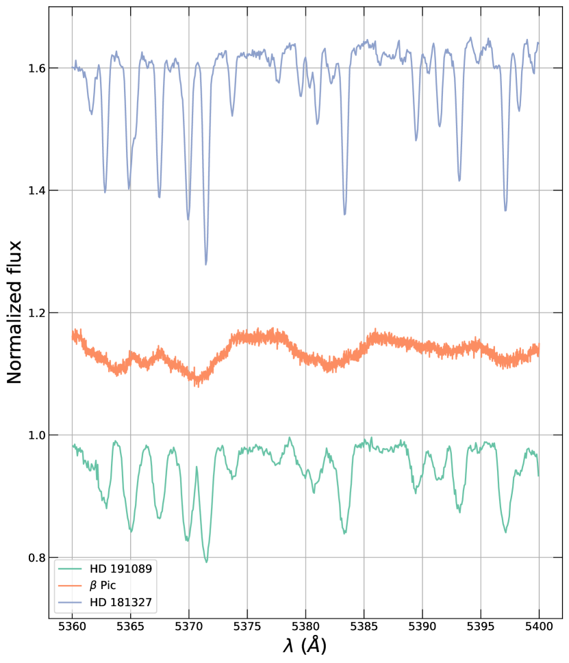
Figure 1: We show the $4500-4540\ \AA$ region of our spectra along with HARPS archival data of $\beta$ Pic from observing program ID 0104.C-0418(C). The high rotational velocities of HD 191089 ($\approx 40$ km.s^-1, Zúñiga-Fernández et al., 2021) and $\beta$ Pic are visible, and individual important atomic features are not possible to distinguish.

Table 1: Log of Magellan/MIKE Observations

ID	R.A.	Decl.	UT Date	Start	Slit	Exposure	$v_{r}$	S/N	S/N	Spectral Type
Designation	(h:m:s)	(d:m:s)			Width	Time (s)	(km s-1)	$4500\ \rm{\AA}$	$6500\ \rm{\AA}$
HD 181327	19:22:58.94	-54:32:16.98	2022 Apr 26	09:37:05	0$\farcs$7	$70$	$-21.8$	$220$	$335$	F$7$
HD 191089	20:09:05.22	-26:13:26.52	2022 Apr 28	09:16:23	0$\farcs$7	$120$	$-33.6$	$300$	$380$	F$5^{a}$

Note. — a: Spectral type from Miret-Roig et al. (2020)

3 Stellar Parameters

We derive photospheric and fundamental stellar parameters for our program star using the algorithm described in Reggiani et al. (2022) that makes use of both the classical spectroscopy-only approach and isochrones to infer accurate, precise, and self-consistent photospheric (T${}_{\text{eff}}$, log$g$, and [Fe/H)] and fundamental (mass, luminosity, and radius) stellar parameters.

For our isochrone fitting we use high-quality multiwavelength photometry from the ultraviolet to the near-infrared: Tycho-2 BT and VT (Høg et al., 2000), Gaia DR2 (Gaia Collaboration et al., 2016, 2018; Arenou et al., 2018; Evans et al., 2018; Hambly et al., 2018; Riello et al., 2018; Gaia Collaboration et al., 2021; Fabricius et al., 2021; Lindegren et al., 2021a, b; Torra et al., 2021) G, J, H, and Ks bands from the Two Micron All Sky Survey (2MASS) All-Sky Point Source Catalog (PSC, Skrutskie et al., 2006), and W1 and W2 bands from the Wide-field Infrared Survey Explorer (WISE) AllWISE mid-infrared data (Wright et al., 2010; Mainzer et al., 2011). We also include Gaia DR3 (Gaia Collaboration et al., 2021) parallax-based distances (Bailer-Jones et al., 2021) of our targets. We include the extinction $A_{V}$ inference based on three-dimensional (3D) maps of extinction in the solar neighborhood from the Structuring by Inversion the Local Interstellar Medium (Stilism) program (Lallement et al., 2014, 2018; Capitanio et al., 2017).

For the spectroscopic-based inferences we use the equivalent widths (EWs) of Fe I and Fe II atomic absorption lines. The EWs were measured from our MIKE spectrum using Gaussian profiles with the splot task of IRAF. The atomic absorption line data is an updated version from the lines described in Yana Galarza et al. (2019). We assume Asplund et al. (2021) photospheric solar abundances.

As described in detail in Reggiani et al. (2022), we use the isochrones package (Morton, 2015) to fit the MESA Isochrones and Stellar Tracks (MIST; Dotter, 2016; Choi et al., 2016; Paxton et al., 2011, 2013, 2015, 2018, 2019) library to our photospheric stellar parameters as well as our input multiwavelength photometry, parallax, and extinction data using MultiNest (Feroz & Hobson, 2008; Feroz et al., 2009, 2019) via PyMultinest (Buchner et al., 2014).

We also analyzed the rotational period using TESS data and the technique of Healy & McCullough (2020); Healy et al. (2021, 2023). We processed PCA-detrended light curves from eleanor (Feinstein et al., 2019) by masking transits, removing outliers, flattening the light curves using 1-D polynomials, and binning the resulting points. We then generated a Lomb-Scargle periodogram and an autocorrelation function for each light curve, analyzing the peak positions and widths to determine periods and uncertainties.

Our adopted stellar parameters ($\rm{T_{eff}}$ and surface gravity from the isochrone analysis, and [Fe/H] and $\xi$ inferred from the atomic Fe I and Fe II lines) are in Table 2. All of the uncertainties quoted in Table 2 include random uncertainties only. That is, they are uncertainties derived under the unlikely assumption that the MIST isochrone grid we use in our analyses perfectly reproduces all stellar properties.

Table 2: Adopted Stellar Parameters for HD 181327

Property	Value	Unit
Tycho $B$	$7.588\pm 0.016$	Vega mag
Tycho $V$	$7.091\pm 0.010$	Vega mag
Gaia DR2 $G$	$6.936\pm 0.002$	Vega mag
2MASS $J$	$6.200\pm 0.024$	Vega mag
2MASS $H$	$5.980\pm 0.044$	Vega mag
2MASS $K_{\text{s}}$	$5.910\pm 0.029$	Vega mag
WISE W1	$5.877\pm 0.053$	Vega mag
WISE W2	$5.792\pm 0.023$	Vega mag
Gaia DR3 parallax	$20.931\pm 0.029$	mas
Isochrone-inferred parameters
Effective temperature $T_{\text{eff}}$	$6498^{+56}_{-53}$	K
Surface gravity $\log{g}$	$4.33\pm 0.01$	cm s-2
Stellar mass $M_{\ast}$	$1.36\pm 0.02$	$M_{\odot}$
Stellar radius $R_{\ast}$	$1.32\pm 0.01$	$R_{\odot}$
Luminosity $L_{\ast}$	$0.44\pm 0.02$	$L_{\odot}$
Isochrone-based age $\tau_{\text{iso}}$	$60\pm 30$	Myr
Spectroscopically inferred parameters
Metallicity $[\text{Fe/H}]$	$0.05\pm 0.06$
Microturbulent velocity $\xi$	$1.63\pm 0.16$	km s-1
Light-curve inferred parameters
Rotational period $P_{\text{rot}}$	$1.542\pm 0.048$	day

4 Elemental Abundances

To infer the elemental abundances of the $\alpha$, light odd-$Z$, iron-peak, and neutron-capture elements we first measure the EWs of atomic absorption lines of Li I, C I, N I, O I, Na I, Mg I, Al I, Si I, S I, K I, Ca I, Sc I, Sc II, Ti I, Ti II, V I, Cr I, Cr II, Mn I, Fe I, Fe II, Ni I, Cu I, Zn I, Y II, and Ba II in our continuum-normalized spectrum by fitting Gaussian profiles with the splot task in IRAF. We use the deblend task to disentangle absorption lines from adjacent spectral features whenever necessary. We measure an EW for every absorption line in our line list that could be recognized, taking into consideration the quality of the spectrum in the vicinity of a line and the availability of alternative transitions of the same species. We assume Asplund et al. (2021) solar abundances and local thermodynamic equilibrium (LTE) and use the 1D plane-parallel solar-composition ATLAS9 (Castelli & Kurucz, 2003) model atmospheres and the 2019 version of the LTE radiative transfer code MOOG to infer elemental abundances based on our EWs.

We report in Table 3 our abundance inferences in three common systems: $A(\text{X})$, $[\text{X/H}]$, and $[\text{X/Fe}]$. We define the uncertainty in the abundance ratio $\sigma_{[\text{X/H}]}$ as the square root of the sum of the square as the standard deviation of the individual line-based abundance inferences $\sigma_{[\text{X/H}]}^{\prime}$ divided by $\sqrt{n_{\text{X}}}$. We define the uncertainty $\sigma_{[\text{X/Fe}]}$ as the square root of the sum of squares of $\sigma_{[\text{X/H}]}$ and $\sigma_{[\text{Fe/H}]}$.

Table 3: Elemental Abundances HD 181327

Species	$A(\text{X})$	[X/H]	$\sigma_{\text{[X/H]}}$	[X/Fe]	$\sigma_{[\text{X/Fe}]}$	$n$
LTE abundances
Li I	$3.49$	$2.53$	$\cdots$	$2.48$	$0.04$	$1$
C I	$8.39$	$-0.07$	$0.06$	$-0.12$	$0.04$	$5$
N I	$\leq 7.81$	$\leq-0.02$	$\cdots$	$\leq-0.07$	$\cdots$	$1$
O I	$8.92$	$0.23$	$0.09$	$0.18$	$0.08$	$3$
Na I	$6.20$	$-0.02$	$0.12$	$-0.07$	$0.12$	$2$
Mg I	$7.65$	$0.10$	$0.12$	$0.04$	$0.07$	$5$
Al I	$6.21$	$-0.22$	$0.34$	$-0.28$	$0.24$	$3$
Si I	$7.77$	$0.26$	$0.32$	$0.20$	$0.10$	$12$
S I	$7.20$	$0.08$	$0.26$	$0.02$	$0.19$	$3$
K I	$5.64$	$0.57$	$0.00$	$0.52$	$0.07$	$1$
Ca I	$6.54$	$0.24$	$0.19$	$0.18$	$0.07$	$11$
Sc I	$3.53$	$0.39$	$0.38$	$0.33$	$0.38$	$2$
Sc II	$3.57$	$0.43$	$0.61$	$0.38$	$0.22$	$9$
Ti I	$5.23$	$0.26$	$0.38$	$0.21$	$0.12$	$12$
Ti II	$5.49$	$0.52$	$0.88$	$0.47$	$0.32$	$9$
V I	$4.54$	$0.64$	$0.05$	$0.59$	$0.07$	$2$
Cr I	$5.74$	$0.12$	$0.24$	$0.07$	$0.09$	$11$
Cr II	$5.90$	$0.28$	$0.21$	$0.23$	$0.10$	$7$
Mn I	$5.26$	$-0.16$	$0.30$	$-0.22$	$0.13$	$7$
Fe I	$7.51$	$0.05$	$0.09$	$\cdots$	$\cdots$	$37$
Fe II	$7.63$	$0.17$	$0.15$	$\cdots$	$\cdots$	$15$
Ni I	$6.34$	$0.14$	$0.34$	$0.09$	$0.09$	$17$
Cu I	$4.35$	$0.17$	$0.29$	$0.11$	$0.29$	$2$
Zn I	$4.51$	$-0.05$	$0.08$	$-0.11$	$0.10$	$2$
Y II	$2.70$	$0.49$	$0.62$	$0.43$	$0.36$	$4$
Ba II	$2.79$	$0.52$	$0.22$	$0.47$	$0.15$	$4$
1D non-LTE abundancesa
C I	$8.37$	$-0.09$	$0.06$	$-0.19$	$\cdots$	$1$
O I	$8.56$	$-0.13$	$0.09$	$-0.23$	$\cdots$	$1$
Al I	$6.10$	$-0.33$	$0.36$	$-0.43$	$\cdots$	$2$
Si I	$7.74$	$0.23$	$0.30$	$0.13$	$\cdots$	$12$
K I	$5.14$	$0.07$	$0.00$	$-0.3$	$\cdots$	$1$
Ca I	$6.04$	$-0.26$	$0.06$	$-0.36$	$\cdots$	$2$
Fe I	$7.56$	$0.10$	$0.09$	$\cdots$	$\cdots$	$37$
Fe II	$7.68$	$0.22$	$0.16$	$\cdots$	$\cdots$	$15$
3D non-LTE abundances
Li I	$3.27$	$2.31$	$\cdots$	$2.18$	$0.04$	$1$
C I	$8.38$	$-0.08$	$0.06$	$-0.18$	$\cdots$	$5$
O I	$8.59$	$-0.10$	$0.06$	$-0.20$	$\cdots$	$3$
Additional abundance ratios of interestb
$[\text{Fe/H}]_{\text{1Dnon-LTE}}=+0.13\pm 0.10$
$[\text{(C+O)/H}]_{\text{1DLTE}}=+0.16\pm 0.11$
$[\text{(C+O)/H}]_{\text{1Dnon-LTE}}=-0.22\pm 0.11$
$[\text{(C+O)/H}]_{\text{3Dnon-LTE}}=-0.18\pm 0.08$
$[\text{C/O}]_{\text{1DLTE}}=-0.3\pm 0.11$
$[\text{C/O}]_{\text{1Dnon-LTE}}=+0.04\pm 0.11$
$[\text{C/O}]_{\text{3Dnon-LTE}}=+0.02\pm 0.08$
C/O${}_{\text{1DLTE}}=+0.30\pm 0.11$
C/O${}_{\text{1Dnon-LTE}}=+0.65\pm 0.11$
C/O${}_{\text{3Dnon-LTE}}=+0.62\pm 0.08$

When possible, we update our elemental abundances for departures from LTE (i.e., non-LTE corrections) by linearly interpolating published grids of non-LTE corrections using scipy (Virtanen et al., 2020). We use the publicly available correction tables from Amarsi et al. (2020) for carbon, oxygen, aluminium, and calcium. Silicon corrections are from Amarsi & Asplund (2017), potassium corrections are from Reggiani et al. (2019), and iron corrections are from Amarsi et al. (2016). There is one caveat for our carbon 1D non-LTE corrected abundance. The Amarsi et al. (2020) non-LTE grid only includes one carbon transition: the $6588\ \AA$ transition. This line is visible in our spectrum, but blended with a telluric feature which we have not been able to properly remove. Therefore, we used the mean 1D LTE abundance of all carbon lines (Table 3) to estimate our correction. For oxygen, the grid has a mean correction based on all three lines at the $777$ nm region. We, therefore, use our mean 1D LTE oxygen abundance (Table 3) to estimate the correction. Our reported 3D non-LTE abundances for carbon and oxygen are a nearest neighbor extrapolation based on the Amarsi et al. (2019) grid. Our extrapolations are to values extremely close to the edge of the correction grids, and therefore reliable results. All our non-LTE estimated abundances are presented in Table 3.

We estimated possible systematics in our non-LTE corrections by interpolating oxygen abundance corrections from Bergemann et al. (2021), through the online tool Spectrum Tools. Our interpolation resulted in a mean 1D non-LTE correction of $\Delta\text{A(O)}=-0.18$, considerably different than the 1D non-LTE correction we inferred ($\Delta\text{A(O)}=-0.36$) from Amarsi et al. (2020).

We confirmed our own estimates by interpolating the same corrections using the online tool INSPECT, which is based on the same oxygen model-atom used in Amarsi et al. (2020). For its interpolation process Spectrum Tools does not request line abundances, therefore the interpolated correction is not specific for a line/abundance measurement. It does, however, show the curve of growth from which the result was interpolated. From visual inspection of the curves of growth, the abundance corrections appear higher than what we reported here ($\Delta\text{A(O)}=-0.18$). Nevertheless, because of the uncertainty generated by not being able to directly interpolate our abundances, we chose to adopt the Amarsi et al. (2020), Amarsi et al. (2019) 1D and 3D corrections, respectively.

Even so, we caution the reader of a possible systematic in our oxygen corrections of up to $\approx 0.18$ dex. It is outside the scope of this study to understand the differences between the models that might be responsible for this difference, but we point that if we were to adopt the 1D non-LTE correction from Spectrum Tools, the C/O ratio would be C/O${}_{\text{1Dnon-LTE}}=+0.43$. This different C/O ratio would not, however, change the interpretations of our results (Section 6.2).

Table 4: Atomic data, Equivalent Widths and line Abundances. Full version online.

Wavelength	Species	Excitation Potential	log($gf$)	EW	$\log_{\epsilon}(\rm{X})$
	(Å)		(eV)		(mÅ)
$6154.225$	Na I	$2.102$	$-1.547$	$25.3$	$6.318$
$6160.747$	Na I	$2.104$	$-1.246$	$28.3$	$6.081$
$4571.095$	Mg I	$0.000$	$-5.623$	$87.5$	$7.781$
$4730.040$	Mg I	$4.340$	$-2.389$	$44.0$	$7.610$

Note. — This table is published in its entirety in the machine-readable format. A portion is shown here for guidance regarding its form and content.

5 $\beta$ Pic b Retrieval

5.1 Retrievals for $\beta$ Pic b

We performed spectral retrievals on $\beta$ Pic b, using the GRAVITY and GPI data (GRAVITY Collaboration et al., 2020; Chilcote et al., 2017). Compared to previous work, we re-calibrated the GPI data following the procedures in De Rosa et al. (2020) which improves the photometric precision and reduces systematic errors. We use ATMO, a 1D-2D radiative-convective equilibrium model for planetary atmospheres to generate models of beta Pic b. More comprehensive descriptions of the model can be found in Amundsen et al. (2014); Tremblin et al. (2015, 2016, 2017); Drummond et al. (2016), Goyal et al. (2018), and Goyal et al. (2018).

Table 5: ATMO Retrieval parameters.

Parameter	Posterior
Fit parameters
$[Z/Z$${}_{\odot}]$	0.021${}_{-0.117}^{+0.243}$
$R$pl(RJup,1 mbar)	1.2941${}_{-0.011}^{+0.015}$
cloud opacity ln($\delta$)	3.26${}_{-0.48}^{+0.32}$
log cloud top (bar)	-0.982${}_{-0.162}^{+0.115}$
$\kappa_{IR}$ (cm2/g)	-1.29$\pm$-0.17
$\gamma_{1}$	-3.57${}_{-1.52}^{+1.37}$
Internal Temp (K)	1840${}_{-18}^{+12}$
$[\text{C/H}]$	0.255${}_{-0.150}^{+0.179}$
$[\text{O/H}]$	0.467${}_{-0.158}^{+0.159}$
$\text{A(C)}$	$8.755_{-0.150}^{+0.179}$
$\text{A(O)}$	$9.227_{-0.158}^{+0.159}$
Asplund et al. (2021) Scaled Abundances
$[\text{Fe/H}]$	$0.081^{+0.246}_{-0.124}$
$[\text{C/H}]$	$0.295_{-0.155}^{+0.183}$
$[\text{O/H}]$	$0.537_{-0.163}^{+0.164}$
Inferred parameters
C/O	0.35${}_{-0.03}^{+0.02}$
Mass ($M_{\rm Jup}$)	7.2${}_{-2.5}^{+3.6}$

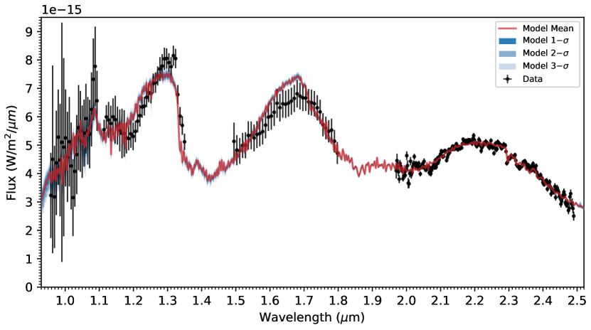
Figure 2: $\beta$ Pic b GPI and Gravity spectrum (black datapoints) along with the posterior distribution of the spectral retrieval model.

For the model assuming chemical equilibrium, the elemental abundances for each model were freely fit and calculated in equilibrium on the fly. Two elements were selected to vary independently, as they are major species which are also likely to be sensitive to spectral features in the data, while the rest were varied by a metallicity parameter ([Z/Z_⊙]). By varying the carbon and oxygen,elemental abundances separately ([C/C_$\odot$] & [O/O_$\odot$]) we allow for non-solar compositions but with chemical equilibrium imposed such that each model fit has a chemically-plausible mix of molecules given the retrieved temperatures, pressures and underlying elemental abundances. In addition, we alleviate an important modeling assumption which can affect the retrieved C/O value (see Drummond et al. 2019). The solar abundances of C, N, O, P, S, K, Fe were defined from Caffau et al. (2011) while we used Asplund et al. (2009) for the other species. As our stellar abundances are scaled to the Asplund et al. (2021) photospheric solar abundances we also present, in Table 5, the planetary metallicity, as traced by iron, carbon, and oxygen abundances re-scaled to the Asplund et al. (2021) solar photospheric abundances. While the solar abundance uncertainties were not included in our original retrieval, we include the uncertainties of the Asplund et al. (2021) solar abundances in Table 5. The updated uncertainties are the square root of the sum of squares of the planetary uncertainties and the Asplund et al. (2021) uncertainties. For the spectral synthesis, we included the spectroscopically active molecules of H₂, He, H₂O, CO₂, CO, CH₄, NH₃, H₂S, HCN, C₂H₂, Na, K, TiO, VO, FeH, Fe, and H-. To parameterize the T-P profile, we use the analytic radiative equilibrium model as described Guillot (2010). We vary three parameters, corresponding to one optical channel, one infrared channel and the internal temperature. The suface gravity was also allowed to vary.

We also included a grey cloud parameterized by a uniform opacity and a cloud top pressure level. Rainout of condensate species was also included. In total, 10 free parameters were used to fit the 337 datapoints. The results are shown in Figs. 2 and 3 with the results also given in Table 5 including the best-fitting model parameters and 1 $\sigma$ uncertainties. We retrieve a mass of 7.2${}_{-2.5}^{+3.6}$ $M_{Jup}$ which consistent with the latest estimates of 9 to 11 $M_{Jup}$ using radial velocity, astrometry, and direct imaging data Feng et al. (2022); Lagrange et al. (2019).

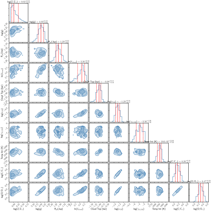
Figure 3: Posterior distribution for the ATMO atmospheric retrieval model fit to the $\beta$ Pic b spectrum.

6 Discussion

6.1 HD 181327 as a Tracer of the Composition of $\beta$ Pic b’s Proto-Planetary Disk

The inferred metallicity of $\beta$ Pic is subsolar (Saffe et al., 2021). Although technically not impossible, it is very unlikely for a solar neighborhood, younger than 100 Myrs star, to be formed in a low metallicity environment (e.g. Kobayashi et al., 2020). On the other hand, the chemical abundances we inferred for HD 181327 are within the expected range of abundances for a solar neighborhood, solar/mildly super-solar metallicity star (both observationally and theoretically, Kobayashi et al., 2020), unlike $\beta$ Pic itself. This difference is a result of $\beta$ Pic’s chemical peculiarities, (see Section 1 and the brief discussion on A stars). This provides initial, albeit indirect, evidence that HD 181327 might be a better representation of the composition of the molecular cloud from which $\beta$ Pic, and $\beta$ Pic b formed.

Stars are formed in clusters, and moving groups are remnants of the clusters where stars were formed. There is now ample evidence indicating that stars formed together are chemically homogeneous. Previous studies of co-moving pairs of stars show that their abundances are homogeneous at the $0.05$ dex level (e.g., Hawkins et al., 2020; Nelson et al., 2021).

Studying open clusters homogeneity, Poovelil et al. (2020) recently found that their chemistry is homogeneous at the $0.03$ dex level. They used APOGEE to study a set of ten open clusters. Each open cluster has at least 13 members (ranging from 13 to 381 members), with an average of 29 members per cluster, excluding the one cluster with 381 studied members (the only cluster with more than 60 members in their sample). This extremely good homogeneity has previously been reported in other open clusters as well: IC 4756 has a star-to-star variation smaller than [X/H]$<0.03$ dex (Ting et al., 2012, e.g.,); The Hyades are homogeneous within $0.02$ dex (De Silva et al., 2006a, b; Liu et al., 2016); M67, NGC 6819, and NGC 2420 also show homogeneity within $0.03$ dex (Bovy, 2016); Bertran de Lis et al. (2016) found homogeneity better than $0.01$ dex for [O/Fe] in several clusters. In conclusion, it is safe to assume that open clusters are homogeneous. Consequently, we can assume that stars in the same moving group are chemically homogeneous at least to the $0.03$ dex level.

Miret-Roig et al. (2020) found 26 members of $\beta$ Pic’s moving group, a similar number of members as those of the Poovelil et al. (2020) open clusters study. With a number of members similar to the previously studied clusters, we assume the homogeneity of the $\beta$ Pic moving group to be similar (dispersion $<0.03$ dex). Therefore, if one can measure the chemical abundances of a reliable tracer of the moving group, its abundances should be within the order of $\sim 0.03$ dex of the remaining moving group members. Thus, the abundances inferred for HD 181327 should be a good reflection of the abundances of the molecular cloud where the $\beta$ Pic moving group formed.

That is not the case for $\beta$ Pic itself. It is an A star with an unusual chemical composition: sub-solar (in [X/H]) abundances of C, Mg, Al, Si, Sc, Ti, Cr, Mn, Fe, and Sr, while showing solar abundance of Mg II, Y, and Ba, and super-solar abundance of Ca (Saffe et al., 2021). $\beta$ Pic is also classified as a $\delta$ Scuti star, with over 30 $\delta$ Scuti pulsation frequencies identified (Mékarnia et al., 2017). The pulsation alone makes it challenging for an abundance analysis, as spectroscopic line-profiles vary with pulsation (Aerts et al., 2008). Moreover, its high rotational velocity ($>100\ \mathrm{km.s^{-1}}$, see Fig. 1) makes it challenging for an accurate and precise determination of several species, such as oxygen (never directly inferred from $\beta$ Pic). In fact, because of the difficulties, and intrinsic characteristics of $\beta$ Pic, a comparison between its composition and the composition we inferred for HD 181327 shows differences far exceeding the $0.03$ dex homogeneity observed in stars formed within the same molecular clouds. We show these differences in Figure 4. Because the inferred chemistry of $\beta$ Pic cannot be reliably used as a proxy for its molecular cloud (due to its pulsation, rotational velocity, and chemical peculiarities), we turned ourselves to another proxy: Hd 181327.

Based on the information presented above, we argue that, for the specific case of $\beta$ Pic b, the best way to interpret its planetary retrieved chemistry is to analyze the chemical makeup of star HD 181327, the only slow rotator, low activity, F star in $\beta$ Pic’s moving group amenable to the analysis we perform in this study, and for which both carbon and oxygen (among other elements) can be accurately inferred. When it comes to the remaining members of $\beta$ Pic’s moving group, to the best of our knowledge, there are no non-LTE, or 3D, carbon and oxygen abundance corrections available for M stars, and any analysis are therefore not as accurate as that of F stars. Thus, not only the analysis of HD 181327 is a better representation of $\beta$ Pic b’s protoplanetary disk than $\beta$ Pic, but also the only analysis that allows us to accurately and precisely infer the abundances of key species such as carbon and oxygen in a well understood stellar context.

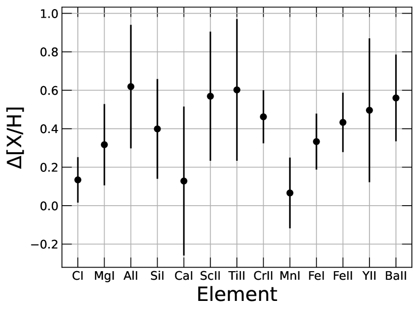
Figure 4: We show the abundance differences between HD 181327 and $\beta$ Pic. The abundances from $\beta$ Pic are from Saffe et al. (2021).

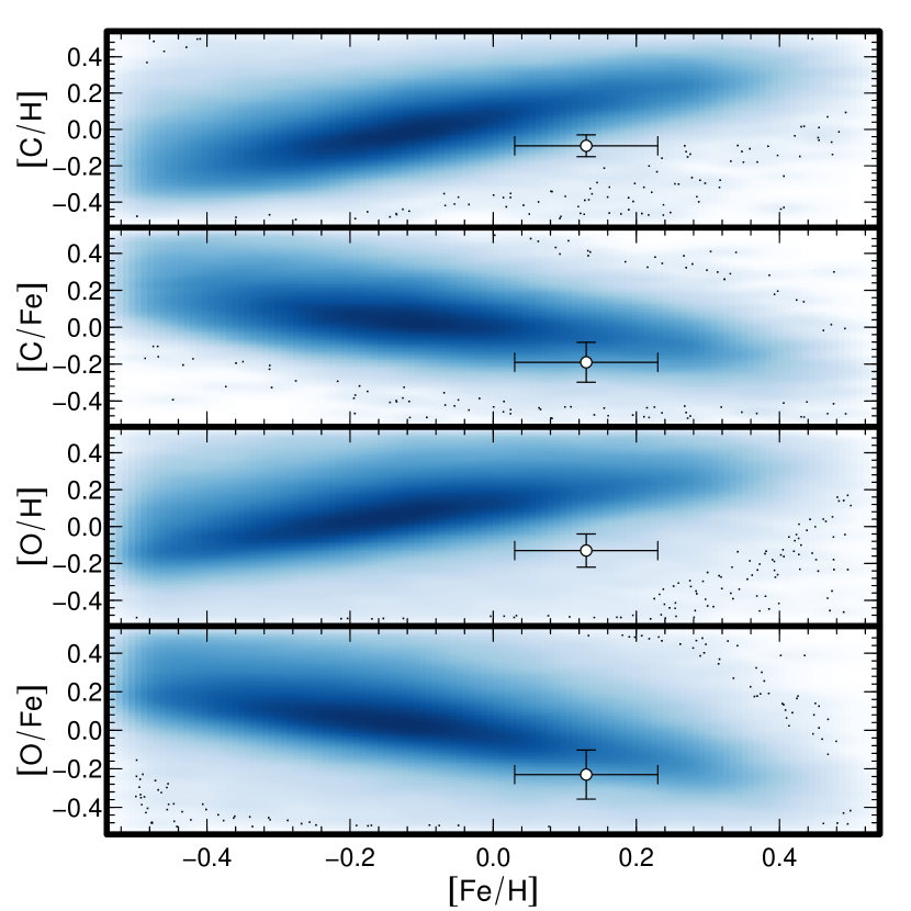
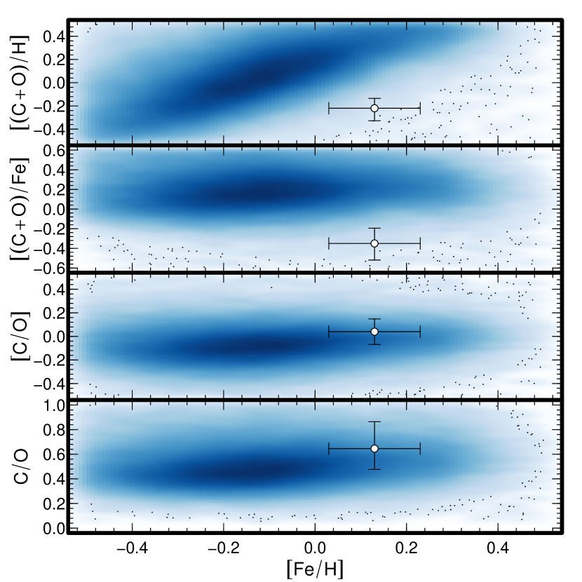
Figure 5: We present, as blue points, the distribution of carbon and oxygen abundances (in different scales) as a function of metallicity from the GALAH DR3 survey. In white we show the abundance of HD 181327, as a proxy for $\beta$ Pic’s molecular cloud. One can see that its abundance is outside of the most populated region in all abundance spaces. This shows the importance of individually determining the stellar abundances for the interpretation of planetary retrievals.

GRAVITY Collaboration et al. (2020) made an extensive discussion of $\beta$ Pic b formation scenario based on the assumption that $\beta$ Pic’s C/O ratio is solar (C/O$=0.59$, from Asplund et al., 2021), and according to them: A subsolar C/O ratio (i.e., $\approx$ 0.4) would invalidate most of the discussion regarding the formation of $\beta$ Pic b. In Figure 5 we show the distribution of carbon and oxygen ratios in the solar neighborhood, using data from the third data release of the Galactic Archaeology with HERMES (GALAH) survey (Buder et al., 2021), and in white the abundances of HD 181327. It is clear from Figure 5 that the abundances of HD 181327 are not located in the bulk of the solar neighborhood distribution. From GALAH, the peak of the distribution of C/O ratios at solar metallicity, in the solar neighborhood, is $\sim 0.1$ dex below solar (C/O$=0.49^{+0.15}_{-0.12}$). Thus, for a solar neighborhood, solar metallicity star, it is more likely to find subsolar than solar abundance for the C/O ratio, and this fact must be taken into account when analyzing planetary abundance information.

As one needs to interpret planetary formation and migration processes taking into account the composition of the disk from which the planet formed (e.g., Reggiani et al., 2022), we propose that the interpretation of planetary abundances should be done in light of:

1. Preferably through the photospheric abundances of the host star.

2. The photospheric abundance of a star formed within the same molecular cloud as the host star/planet.

3. The mean abundances observed in the Galactic substructure where we observe the planet (solar neighborhood).

4. If all other options are not possible, one should assume solar abundances.

For the photosphere of HD 181327, and therefore the protoplanetary disk from which $\beta$ Pic b formed, we found (3D non-LTE corrected abundances) [C/H]$=-0.08\pm 0.06$, [O/H]$=-0.10\pm 0.06$, [(C+O)/H]$=-0.18\pm 0.08$, C/O]$=+0.02\pm 0.08$, and C/O$=+0.62\pm 0.08$. We will discuss $\beta$ Pic b’s formation using the 3D non-LTE abundances calculations as the basis of our discussions. We reinforce that our carbon 1D LTE, 1D non-LTE, and 3D non-LTE abundances are all compatible, and the differences between them are smaller than the uncertainties.

6.2 The Formation of $\beta$ Pic b

Our retrieval of $\beta$ Pic b yields different results than those reported by the GRAVITY Collaboration et al. (2020). We attribute the differences mostly to our updated methodology in the GPI data reduction. Compared to the GRAVITY Collaboration et al. (2020) retrieval, our metallicities are in much better agreement to the stellar results. The 1D non-LTE metallicity of the planetary disk, as traced by HD 181327, is [Fe/H]${}_{\text{1DNLTE}}=+0.13\pm 0.10$, and the planetary metallicity is [Fe/H]$=0.5$, and [Fe/H]$=+0.08^{+0.25}_{-0.12}$ from GRAVITY Collaboration et al. (2020) and our own retrieval, respectively. Ours is a clear improvement as it is now fully reconciled to the metallicity traced by the stellar information recorded in HD 181327. Not only that, but the much lower metallicity we inferred is much more amenable to the core-accretion formation scenario of $\beta$ Pic $b$, than the [Fe/H]$=0.5$ dex previously inferred.

Our retrieved C/O abundance ratio is smaller than what was previously reported, although there is agreement within the quoted uncertainties (C/O$=+0.35^{+0.02}_{-0.03}$ from us and C/O$=0.43\pm 0.05$ from GRAVITY Collaboration et al. (2020)). The GRAVITY Collaboration et al. (2020) team, however, did not report the individual carbon and oxygen abundances, as carbon in their retrieval was scaled to the planetary metallicity, and oxygen was freely varied to recover the inferred C/O ratio. In our retrieval the abundances are estimated on the fly and every element retrieved is treated as a free parameter. Therefore, our carbon and oxygen abundances are not biased by the assumption of solar scaled [C/H].

We present in Figure 6 the retrieved $(\textrm{C/O})_{\textrm{Planet}}/(\textrm{C/O})_{\textrm{Star}}$ as a function of $\textrm{A(C)}_{\textrm{Planet}}/\textrm{A(C)}_{\textrm{Star}}$ and as a function of $\textrm{A(O)}_{\textrm{Planet}}/\textrm{A(O)}_{\textrm{Star}}$, for both ours and GRAVITY Collaboration et al. (2020) retrievals. We present in both cases the abundances assuming solar C/O and carbon and oxygen for the host star, and our inference from HD 181327. In both panels we outline the different possible formation scenarios as described in the model presented by Öberg et al. (2011).

As already pointed by GRAVITY Collaboration et al. (2020) we have little information about the relationship between the current orbit of $\beta$ Pic b and its formation location, and about possible variations of the locations of the ice lines in systems such as that of $\beta$ Pic (no direct observations of the ice lines in $\beta$ Pic have been made to the best of our knowledge). However, based on the formation model presented by Öberg et al. (2011), our results indicate $\beta$ Pic b formed beyond the H₂O ice line by accreting large ammounts of icy planetesimals after envelope accretion.

Even though we obtained different results in our planetary retrieval (see the metallicity difference), our stellar and planetary analysis corroborates the discussion presented by the Gravity Team. GRAVITY Collaboration et al. (2020) inferred $\beta$ Pic b’s atmospheric C/O ratio is indicative $\beta$ Pic b slowly formed between the H₂O and CO₂ ice lines, via core-accretion. Its substellar C/O can be explained if the planet was enriched in oxygen by icy planetesimals. For more complete calculations we refer the reader to their study. We would also like to point out that even with the possible maximum systematic differences in the stellar non-LTE corrections from Bergemann et al. (2021) (stellar C/O$=+0.43$) the conclusions drawn are the same. The planet would be located in the same quadrant as is in Figure 6. We have, therefore, strong evidence on the formation scenario of this planet, as all results converge regardless of analysis (two different planetary atmospheric retrievals, and different assumptions to the composition of its protoplanetary disk pointing to the same conclusion).

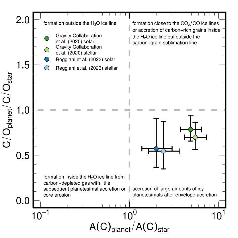
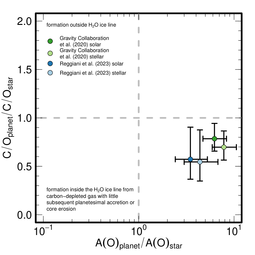
Figure 6: On the left we present the planetary to stellar (protoplanetary disk proxy) C/O ratios of $\beta$ Pic b as a function of planet to stellar carbon abundances, and on the right we present the planetary to stellar C/O ratios as a function of planetary to stellar oxygen abundance. In dark and light green we present the planetary results of the GRAVITY Collaboration et al. (2020) study, scaled to solar and stellar (HD 181327) abundances, respectively. In dark and light blue we present the same, but for the carbon and oxygen abundances retrieved for $\beta$ Pic b from our study. We see that regardless of the retrieval there is a difference in using solar and stellar abundances, portraying the importance of a dedicated stellar analysis. It is also clear that our retrieval has considerably changed the results. While there are visible differences, for $\beta$ Pic b our different analysis corroborate previsous conclusions about the planetary formation. It formed beyond the H₂O ice-line, accreting large amounts of icy planetesimals after envelope accretion.

7 Conclusion

We find that the chemical pattern of HD 181327, a member of the $\beta$ Pic moving group, can be reliably used as a proxy to infer the chemical content of the molecular cloud form which $\beta$ Pic was formed. As such, and considering the abundances of $\beta$ Pic itself are not a reliable representation of its parent molecular cloud because of its intrinsic characteristics, we argue that the composition of the Hot Jupiter $\beta$ Pic b should be interpreted in light of HD 181327 composition.

We enumerate what we argue to be the most reliable ways to infer the composition of the protoplanetary disks from which exoplanets formed.

We also performed our own retrieval of the parameters and abundances of $\beta$ Pic b. We retrieved a planetary metallicity that is fully in agreement to the abundance of HD 181327. We present carbon and oxygen abundances for both star and planet (stellar abundances are 3D non-LTE corrected). Our stellar C/O ratio is close to solar, but we found an important discrepancy in the abundances (in articular the metallicity) from our retrieval and the retrieval by GRAVITY Collaboration et al. (2020). We attribute the differences to the our updated (recalibrated) data reduction pipeline. The combination of our stellar analysis and planetary retrieval indicate $\beta$ Pic. $b$ formed beyond the H₂O ice-line, and accreted large amounts of icy planetesimals after envelope accretion. It is important to point that our updated retrieval along with a new stellar analysis arrived at the same conclusion as previous studies, corroborating their conclusions and strongly reinforcing the proposed scenario for the formation of $\beta$ Pic $b$.

References

- Aerts et al. (2008) Aerts, C., Hekker, S., Desmet, M., et al. 2008, in Precision Spectroscopy in Astrophysics, ed. N. C. Santos, L. Pasquini, A. C. M. Correia, & M. Romaniello, 161–164, doi: 10.1007/978-3-540-75485-5_35
- Ali-Dib (2017) Ali-Dib, M. 2017, MNRAS, 467, 2845, doi: 10.1093/mnras/stx260
- Ali-Dib et al. (2014) Ali-Dib, M., Mousis, O., Petit, J.-M., & Lunine, J. I. 2014, ApJ, 785, 125, doi: 10.1088/0004-637X/785/2/125
- Amarsi & Asplund (2017) Amarsi, A. M., & Asplund, M. 2017, MNRAS, 464, 264, doi: 10.1093/mnras/stw2445
- Amarsi et al. (2016) Amarsi, A. M., Lind, K., Asplund, M., Barklem, P. S., & Collet, R. 2016, MNRAS, 463, 1518, doi: 10.1093/mnras/stw2077
- Amarsi et al. (2019) Amarsi, A. M., Nissen, P. E., & Skúladóttir, Á. 2019, A&A, 630, A104, doi: 10.1051/0004-6361/201936265
- Amarsi et al. (2020) Amarsi, A. M., Lind, K., Osorio, Y., et al. 2020, A&A, 642, A62, doi: 10.1051/0004-6361/202038650
- Amundsen et al. (2014) Amundsen, D. S., Baraffe, I., Tremblin, P., et al. 2014, A&A, 564, A59, doi: 10.1051/0004-6361/201323169
- Andrews et al. (2019) Andrews, J. J., Anguiano, B., Chanamé, J., et al. 2019, ApJ, 871, 42, doi: 10.3847/1538-4357/aaf502
- Andrievsky et al. (2002) Andrievsky, S. M., Chernyshova, I. V., Paunzen, E., et al. 2002, A&A, 396, 641, doi: 10.1051/0004-6361:20021423
- Arenou et al. (2018) Arenou, F., Luri, X., Babusiaux, C., et al. 2018, A&A, 616, A17, doi: 10.1051/0004-6361/201833234
- Asplund et al. (2021) Asplund, M., Amarsi, A. M., & Grevesse, N. 2021, A&A, 653, A141, doi: 10.1051/0004-6361/202140445
- Asplund et al. (2009) Asplund, M., Grevesse, N., Sauval, A. J., & Scott, P. 2009, ARA&A, 47, 481, doi: 10.1146/annurev.astro.46.060407.145222
- Astropy Collaboration et al. (2013) Astropy Collaboration, Robitaille, T. P., Tollerud, E. J., et al. 2013, A&A, 558, A33, doi: 10.1051/0004-6361/201322068
- Astropy Collaboration et al. (2018) Astropy Collaboration, Price-Whelan, A. M., Sipőcz, B. M., et al. 2018, AJ, 156, 123, doi: 10.3847/1538-3881/aabc4f
- Bailer-Jones et al. (2021) Bailer-Jones, C. A. L., Rybizki, J., Fouesneau, M., Demleitner, M., & Andrae, R. 2021, AJ, 161, 147, doi: 10.3847/1538-3881/abd806
- Balmer et al. (2023) Balmer, W. O., Pueyo, L., Stolker, T., et al. 2023, arXiv e-prints, arXiv:2309.04403, doi: 10.48550/arXiv.2309.04403
- Bergemann et al. (2021) Bergemann, M., Hoppe, R., Semenova, E., et al. 2021, MNRAS, 508, 2236, doi: 10.1093/mnras/stab2160
- Bernstein et al. (2003) Bernstein, R., Shectman, S. A., Gunnels, S. M., Mochnacki, S., & Athey, A. E. 2003, in Society of Photo-Optical Instrumentation Engineers (SPIE) Conference Series, Vol. 4841, Proc. SPIE, ed. M. Iye & A. F. M. Moorwood, 1694–1704, doi: 10.1117/12.461502
- Bertran de Lis et al. (2016) Bertran de Lis, S., Allende Prieto, C., Majewski, S. R., et al. 2016, A&A, 590, A74, doi: 10.1051/0004-6361/201527827
- Beust & Morbidelli (2000) Beust, H., & Morbidelli, A. 2000, Icarus, 143, 170, doi: 10.1006/icar.1999.6238
- Booth et al. (2017) Booth, R. A., Clarke, C. J., Madhusudhan, N., & Ilee, J. D. 2017, MNRAS, 469, 3994, doi: 10.1093/mnras/stx1103
- Bovy (2016) Bovy, J. 2016, ApJ, 817, 49, doi: 10.3847/0004-637X/817/1/49
- Buchner et al. (2014) Buchner, J., Georgakakis, A., Nandra, K., et al. 2014, A&A, 564, A125, doi: 10.1051/0004-6361/201322971
- Buder et al. (2021) Buder, S., Sharma, S., Kos, J., et al. 2021, MNRAS, 506, 150, doi: 10.1093/mnras/stab1242
- Caffau et al. (2011) Caffau, E., Ludwig, H. G., Steffen, M., Freytag, B., & Bonifacio, P. 2011, Sol. Phys., 268, 255, doi: 10.1007/s11207-010-9541-4
- Cánovas et al. (2019) Cánovas, H., Cantero, C., Cieza, L., et al. 2019, A&A, 626, A80, doi: 10.1051/0004-6361/201935321
- Capitanio et al. (2017) Capitanio, L., Lallement, R., Vergely, J. L., Elyajouri, M., & Monreal-Ibero, A. 2017, A&A, 606, A65, doi: 10.1051/0004-6361/201730831
- Casagrande et al. (2021) Casagrande, L., Lin, J., Rains, A. D., et al. 2021, MNRAS, 507, 2684, doi: 10.1093/mnras/stab2304
- Casey (2014) Casey, A. R. 2014, PhD thesis, Australian National University, Canberra
- Castelli & Kurucz (2003) Castelli, F., & Kurucz, R. L. 2003, in Modelling of Stellar Atmospheres, ed. N. Piskunov, W. W. Weiss, & D. F. Gray, Vol. 210, A20, doi: 10.48550/arXiv.astro-ph/0405087
- Chilcote et al. (2017) Chilcote, J., Pueyo, L., De Rosa, R. J., et al. 2017, AJ, 153, 182, doi: 10.3847/1538-3881/aa63e9
- Choi et al. (2016) Choi, J., Dotter, A., Conroy, C., et al. 2016, ApJ, 823, 102, doi: 10.3847/0004-637X/823/2/102
- Cridland et al. (2019a) Cridland, A. J., Eistrup, C., & van Dishoeck, E. F. 2019a, A&A, 627, A127, doi: 10.1051/0004-6361/201834378
- Cridland et al. (2016) Cridland, A. J., Pudritz, R. E., & Alessi, M. 2016, MNRAS, 461, 3274, doi: 10.1093/mnras/stw1511
- Cridland et al. (2019b) Cridland, A. J., van Dishoeck, E. F., Alessi, M., & Pudritz, R. E. 2019b, A&A, 632, A63, doi: 10.1051/0004-6361/201936105
- Cridland et al. (2020) —. 2020, A&A, 642, A229, doi: 10.1051/0004-6361/202038767
- Crifo et al. (1997) Crifo, F., Vidal-Madjar, A., Lallement, R., Ferlet, R., & Gerbaldi, M. 1997, in ESA Special Publication, Vol. 402, Hipparcos - Venice ’97, ed. R. M. Bonnet, E. Høg, P. L. Bernacca, L. Emiliani, A. Blaauw, C. Turon, J. Kovalevsky, L. Lindegren, H. Hassan, M. Bouffard, B. Strim, D. Heger, M. A. C. Perryman, & L. Woltjer, 437–440
- Crozet et al. (2023) Crozet, P., Morin, J., Ross, A. J., et al. 2023, arXiv e-prints, arXiv:2310.04497, doi: 10.48550/arXiv.2310.04497
- De Rosa et al. (2020) De Rosa, R. J., Esposito, T. M., Gibbs, A., et al. 2020, in Society of Photo-Optical Instrumentation Engineers (SPIE) Conference Series, Vol. 11447, Society of Photo-Optical Instrumentation Engineers (SPIE) Conference Series, 114475A, doi: 10.1117/12.2561071
- De Silva et al. (2006a) De Silva, G. M., Sneden, C., Paulson, D. B., et al. 2006a, AJ, 131, 455, doi: 10.1086/497968
- De Silva et al. (2006b) —. 2006b, AJ, 131, 455, doi: 10.1086/497968
- Dotter (2016) Dotter, A. 2016, ApJS, 222, 8, doi: 10.3847/0067-0049/222/1/8
- Drummond et al. (2019) Drummond, B., Carter, A. L., Hébrard, E., et al. 2019, MNRAS, 486, 1123, doi: 10.1093/mnras/stz909
- Drummond et al. (2016) Drummond, B., Tremblin, P., Baraffe, I., et al. 2016, A&A, 594, A69, doi: 10.1051/0004-6361/201628799
- Eistrup et al. (2018) Eistrup, C., Walsh, C., & van Dishoeck, E. F. 2018, A&A, 613, A14, doi: 10.1051/0004-6361/201731302
- Espinoza et al. (2017) Espinoza, N., Fortney, J. J., Miguel, Y., Thorngren, D., & Murray-Clay, R. 2017, ApJ, 838, L9, doi: 10.3847/2041-8213/aa65ca
- Evans et al. (2018) Evans, D. W., Riello, M., De Angeli, F., et al. 2018, A&A, 616, A4, doi: 10.1051/0004-6361/201832756
- Fabricius et al. (2021) Fabricius, C., Luri, X., Arenou, F., et al. 2021, A&A, 649, A5, doi: 10.1051/0004-6361/202039834
- Feinstein et al. (2019) Feinstein, A. D., Montet, B. T., Foreman-Mackey, D., et al. 2019, PASP, 131, 094502, doi: 10.1088/1538-3873/ab291c
- Feng et al. (2022) Feng, F., Butler, R. P., Vogt, S. S., et al. 2022, ApJS, 262, 21, doi: 10.3847/1538-4365/ac7e57
- Ferlet et al. (1987) Ferlet, R., Hobbs, L. M., & Vidal-Madjar, A. 1987, A&A, 185, 267
- Feroz & Hobson (2008) Feroz, F., & Hobson, M. P. 2008, MNRAS, 384, 449, doi: 10.1111/j.1365-2966.2007.12353.x
- Feroz et al. (2009) Feroz, F., Hobson, M. P., & Bridges, M. 2009, MNRAS, 398, 1601, doi: 10.1111/j.1365-2966.2009.14548.x
- Feroz et al. (2019) Feroz, F., Hobson, M. P., Cameron, E., & Pettitt, A. N. 2019, The Open Journal of Astrophysics, 2, 10, doi: 10.21105/astro.1306.2144
- Folsom et al. (2012) Folsom, C. P., Bagnulo, S., Wade, G. A., et al. 2012, MNRAS, 422, 2072, doi: 10.1111/j.1365-2966.2012.20718.x
- Fulton et al. (2017) Fulton, B. J., Petigura, E. A., Blunt, S., & Sinukoff, E. 2017, RadVel: The Radial Velocity Fitting Toolkit, doi: 10.5281/zenodo.580821
- Fulton et al. (2018) —. 2018, PASP, 130, 044504, doi: 10.1088/1538-3873/aaaaa8
- Gaia Collaboration et al. (2016) Gaia Collaboration, Prusti, T., de Bruijne, J. H. J., et al. 2016, A&A, 595, A1, doi: 10.1051/0004-6361/201629272
- Gaia Collaboration et al. (2018) Gaia Collaboration, Brown, A. G. A., Vallenari, A., et al. 2018, A&A, 616, A1, doi: 10.1051/0004-6361/201833051
- Gaia Collaboration et al. (2021) —. 2021, A&A, 649, A1, doi: 10.1051/0004-6361/202039657
- Galland et al. (2006) Galland, F., Lagrange, A. M., Udry, S., et al. 2006, A&A, 447, 355, doi: 10.1051/0004-6361:20054080
- Galli et al. (2020) Galli, P. A. B., Bouy, H., Olivares, J., et al. 2020, A&A, 634, A98, doi: 10.1051/0004-6361/201936708
- Galli et al. (2019) Galli, P. A. B., Loinard, L., Bouy, H., et al. 2019, A&A, 630, A137, doi: 10.1051/0004-6361/201935928
- García Pérez et al. (2016) García Pérez, A. E., Allende Prieto, C., Holtzman, J. A., et al. 2016, AJ, 151, 144, doi: 10.3847/0004-6256/151/6/144
- Goyal et al. (2018) Goyal, J. M., Mayne, N., Sing, D. K., et al. 2018, MNRAS, 474, 5158, doi: 10.1093/mnras/stx3015