Comparing self-consistent $GW$ and vertex corrected $G_{0}W_{0}$ ($G_{0}W_{0}\Gamma$) accuracy for molecular ionization potentials

Abstract

We test the performance of self-consistent $GW$ and several representative implementations of vertex corrected $G_{0}W_{0}$ ($G_{0}W_{0}\Gamma$). These approaches are tested on benchmark data sets covering full valence spectra (first ionization potentials and some inner valence shell excitations). For small molecules, when comparing against state of the art wave function techniques, our results show that performing full self-consistency in the GW scheme either systematically outperforms vertex corrected $G_{0}W_{0}$ or gives results of at least the same quality. Moreover, the $G_{0}W_{0}\Gamma$ results in additional computational cost when compared to $G_{0}W_{0}$ or self-consistent $GW$ and the $G_{0}W_{0}\Gamma$ dependency on the starting mean-filed solution is frequently larger than the magnitude of the vertex correction. Consequently, for molecular systems self-consistent GW performed on imaginary axis and then followed by modern analytical continuation techniques offers a more reliable approach to make predictions of IP spectra.

I Introduction

Accurate and computationally accessible simulation of molecules and periodic solids is a major goal when developing new or improving the existing computational approaches. While wave function methods such as coupled cluster method (CC) ^{1, 2, 3} and configuration interaction (CI) ^{4, 5, 6} have have seen a great success in modeling moderately sized molecular systems and solids with small unit cells with great accuracy, the challenge of ab-initio modelling of realistic periodic systems with moderate/large unit cell sizes remains open. Simulating complex molecules or realistic solids with traditional ab-initio wave function methods is computationally extremely challenging mainly due to the high computational scaling.

To conduct calculations on larger molecules or periodic systems, methods with lower computational scaling are favorable. Approaches such as density functional theory (DFT) ^{7, 8} are more efficient in tackling systems with large numbers of electrons. In solid state physics, DFT has been successfully performed on nearly 3500 atoms. ⁹ However, these methods often struggle to offer quantitatively accurate predictions when electron correlation plays a significant role. Moreover, for the DFT methods there is a lack of a systematic route to improve the results.

Many-body perturbation theory (MBPT) cast into Green’s function language provides an alternative group of ab-initio methods to model electron correlation. ¹⁰ Most of these methods such as $GW$ ^{11, 12, 13, 14, 15, 16, 17, 18, 19, 20, 21} or Green’s function second order (GF2) ^{22, 23, 24, 25, 26} can be executed with relatively low computational scaling especially when compared to the wave function theories.

Since the diagrammatic Green’s function expansions are based on perturbation theory, they also hold a promise of being systematically improvable. In 1965, Hedin proposed a complete set of conjugated equations, detailing the relationships between Green’s function, irreducible polarizability, screened Coulomb interaction, vertex function, and self-energy. ¹¹ The $GW$ method constitutes a simpler truncated formulation of Hedin’s equations of MBPT. The approximate version of $GW$ theory, namely $G_{0}W_{0}$, where only the first iteration of the self-consistency is performed and vertex function is assumed to be unity, has become one of the most widely applied methodologies in the computational electronic structure. While relatively accurate and computationally inexpensive, $G_{0}W_{0}$ still lacks full quantitative accuracy and can qualitatively fail for systems where the correlations become stronger.

One of the proposals of improving $G_{0}W_{0}$ accuracy is the addition of the vertex function $\Gamma$ as a correction term to $G_{0}W_{0}$. Those vertex containing methods are commonly referred to as $G_{0}W_{0}\Gamma$. ^{27, 28, 29, 30, 31, 32, 33, 34} Generally, the vertex correction is expected to address stronger electron correlation in both solids and molecules, and improve predictions for band structure and photo-electron spectrum. However, the detailed implementation, approximations introduced, and performance of $G_{0}W_{0}\Gamma$ vary from one variant to another because many different strategies can be introduced to lower the computational scaling.

Another possible strategy of including more diagrammatic terms than in $G_{0}W_{0}$ would be performing the full self-consistent solution of Hedin’s equations but without an inclusion of the vertex function. Such an approach, called self-consistent $GW$ (sc$GW$), relies on updating the Green’s function $G$ as well as self-energy $\Sigma$ in the $GW$-loop until convergence is reached. The computational scaling of the $GW$ method is $\mathcal{O}(N^{4})$, ^{35, 36} when the density-fitting approximation ³⁷ is used to decompose the two-electron integrals. When compared with $G_{0}W_{0}$, the cost of sc$GW$ differs only by a prefactor involving the number of iterations required to reach convergence. Multiple variants of the $GW$ self-consistency were introduced in the past. For a detailed discussion of these variants see Refs. [20, 38, 39, 35, 36].

Consequently, two proposals can be put forward to add more diagrammatic terms on top of $G_{0}W_{0}$: inclusion of the vertex function directly on top of $G_{0}W_{0}$ resulting in some kind of $G_{0}W_{0}\Gamma$ scheme, or alternatively, performing a fully self-consistent sc$GW$ loop.

The objective of this paper is to investigate the performance of these two routes of the diagrammatic improvement of $G_{0}W_{0}$. These comparisons can guide future numerical developments in Green’s function theories towards robust methods that provide a good compromise between low computational scaling and high accuracy.

To conduct this investigation, we employ our recently introduced finite temperature sc$GW$  method and compare its results against the $G_{0}W_{0}\Gamma$ schemes presented earlier in the literature. Since the full evaluation of the vertex function (as discussed in Sec. II) is very expensive, multiple approximations have been introduced to evaluate the vertex on top of $G_{0}W_{0}$. We compare sc$GW$ against three possible ways of approximating vertex, (i) stochastic methodology developed in the group of Vlček in Ref. [40], (ii) $G_{0}W_{0}\Gamma^{(1)}$ as implemented by Wang et al. and presented in Ref. [31], and (iii) $G_{0}W_{0}\Gamma$ implemented in the Kresse’s group and presented in Ref. [30] by Maggio et al.

sc$GW$ and vertex corrected $G_{0}W_{0}$ methodologies are tested on molecular examples where data can be validated against wave function theories. We focus our discussion on examining these approaches both for the first and inner valence shell ionization potentials (IP).

We present our work in this article as follows. In Section II, we provide a concise introduction to finite temperature sc$GW$ and a brief review of recent developments in adding the vertex correction to $G_{0}W_{0}$. Section III describes the general calculation protocol we used to conduct comparisons. Section IV contains major findings of this work. We summarize our findings and outlooks in Section V.

II Theory

II.1 Hedin’s equations

A set of self-consistent equations detailing the relationship among self-energy, Green’s function, screened Coulomb interaction, and irreducible polarizability in many-electron systems was formulated in the Hedin’s foundational article ¹¹ in 1965.

In the derivation of Hedin’s equations, a bare Coulomb interaction $v$ is affected (or “screened”) by the many-electron environment. The screened Coulomb interaction $W$ is defined as

$$W(12)=v(12)+W(13)P(34)v(42),$$ (1)

where numeric compact indices are employed as a shorthand to represent the state of space-time and spin as $1=(\textbf{x}_{1},\sigma_{1},t_{1}$). Integration over repeated indices is assumed. The irreducible polarizability is defined as

$$P(34)=iG(45)G(64)\frac{\delta G^{-1}(56)}{\delta V(3)},$$ (2)

where $V$ is the time evolution operator. The functional derivative $\frac{\delta G^{-1}(56)}{\delta V(3)}$ is called the vertex function, and expressed as

$$\begin{split}\Gamma(12;3){}&\equiv-\frac{\delta G^{-1}(12)}{\delta V(3)}=\delta(12)\delta(13)+\frac{\delta\Sigma(12)}{\delta V(3)}\\ &=\delta(13)\delta(23)+\frac{\delta\Sigma(12)}{\delta G(45)}G(46)G(75)\Gamma(67;3).\end{split}$$ (3)

The inclusion of vertex function can be viewed as inclusion of information about the interaction between electrons and holes. ^{41, 42}

In the original formulation, evaluating the exact vertex function significantly increases the computational cost because it is difficult to calculate a four-index functional derivative. If the vertex function was truncated at the zeroth order in Eq. (3) as $\Gamma(12;3)\approx\delta(12)\delta(13)$, then self-energy $\Sigma$ and reduced polarizability $P$ can be calculated without evaluating the functional derivative as

$$\begin{split}\Sigma(12){}&=iW(13)G(14)\Gamma(42;3)\\ &\approx iG(12)W(12),\end{split}$$ (4)

$$\begin{split}P(12){}&=-iG(23)G(42)\Gamma(34;1)\\ &\approx-iG(12)G(21).\end{split}$$ (5)

The name $GW$ approximation (GWA) was coined to signify the exclusion of vertex function in the Hedin’s equation ^{11, 14}. The GWA scheme is depicted by the trapezoidal loop in the right diagram shown in Figure 1.

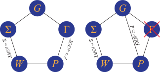
Figure 1: Left: Self-energy, Green’s function, vertex function, irreducible polarizability, and screened Coulomb interaction conjugated by Hedin’s equations. Right: $GW$ approximation loop of Hedin’s equations without inclusion of the vertex function.

II.2 $G_{0}W_{0}$ and self-consistent $GW$

GWA can be executed in two ways. One of them called $G_{0}W_{0}$ is the first iteration of the Hedin’s equations without inclusion of the vertex function where the zeroth order Green’s function $G_{0}$ is evaluated using the mean-field Hamiltonian (Hartree-Fock or DFT) and then used to evaluate the self-energy. Usually, only the diagonal elements of the self-energy matrix are evaluated and the quasiparticle (QP) approximation is then employed to get the spectral quantities. ²¹

Fully self-consistent $GW$ called sc$GW$ is executed if all quantities in the trapezoid describing Hendin’s equations are iterated until self-consistency. For the implementation details of sc$GW$ as performed in the Zgid group, we encourage the reader to consult Ref. [43] for molecular problems, Refs. [44, 36, 45] for periodic problems, and Ref. [46] for relativistic problems in periodic solids.

In our finite temperature sc$GW$ implementation, we express the frequency/time dependent quantities on an imaginary axis grid. ^{47, 48, 49, 50} No diagonal approximation to the self-energy is used and all the matrix elements of self-energy for all the frequencies are evaluated and included in the self-consistent equations. The total self-energy in sc$GW$ is expressed as

$$\tilde{\Sigma}^{GW}[\mathcal{G}](i\omega)={\Sigma}_{\infty}^{GW}[\mathcal{G}]+{\Sigma}^{GW}[\mathcal{G}](i\omega),$$ (6)

where ${\Sigma}_{\infty}^{GW}[\mathcal{G}]$ is the static part of self-energy evaluated using the first order diagrams (Hartree and exchange) employing the correlated one-body density matrix, and ${\Sigma}^{GW}[\mathcal{G}](i\omega)$ is the frequency-dependent dynamical part of self-energy. Both self-energy parts, dynamic and static, depend on Green’s function and are evaluated iteratively until achieving self-consistency.

Overall, the computational cost of our sc$GW$ scales as $\mathcal{O}(N_{\tau}N_{\mathrm{orb}}^{2}N_{\mathrm{aux}}^{2})$, where $N_{\tau}$ is the number of imaginary time grid points, $N_{\mathrm{orb}}$ is the number of orbitals in the problem, and $N_{\mathrm{aux}}$ is the number of auxiliary basis functions used in the density fitting procedure.

No QP approximation is evoked in order to evaluate spectral quantities in our version of sc$GW$. To yield spectral information, the finite-temperature Green’s function from the imaginary axis is continued to the real frequency axis with the help of the Nevanlinna analytical continuation technique introduced by Fei et al. ^{51, 52} The molecular spectral function can be derived from the continued Green’s function as

$$\mathcal{G}(i\omega)\xrightarrow[\mathrm{analytical\ continuation}]{\mathrm{Nevanlinna}}A(\omega)=-\frac{1}{\pi}\mathrm{Im}\left[\mathrm{Tr[}G(\omega)]\right].$$ (7)

Spectral functions rendered by Nevanlinna continuation are positive and normalized by definition, which helps to resolve the isolated ionization peaks in PES.

II.3 Practical implementations of vertex correction

It is believed that introducing vertex function $\Gamma$ as a correction term on top of GWA can improve its accuracy. The rigorous evaluation of vertex function is difficult due to the presence of a four-point functional derivative ($\delta\Sigma/\delta G$) in Eq. 3 and due to the necessity of iterative self-consistent evaluation of both self-energy $\Sigma$ and irreducible polarizability $P$ since they involve $\Gamma$ in their respective Eqs. (4) and (5). Consequently, in practical implementations of the vertex correction many approximations are introduced to lower the computational cost and make such evaluations viable.

It is frequently argued that sc$GW$ overestimates band gaps. ^{19, 53} Thus $G_{0}W_{0}$, which benefits from the error cancellation between the DFT starting point and a subsequent $GW$ evaluation, is used as an affordable alternative. In this approximation, $\Gamma$ is evaluated on top of $G_{0}W_{0}$ resulting in a $G_{0}W_{0}\Gamma$ method. However, even in this simplified scenario further approximations are necessary to make the final evaluation of $G_{0}W_{0}\Gamma$ possible. Here, we summarize recent developments of practical $G_{0}W_{0}\Gamma$ implementations.

Reining and coworkers introduced the $\rho/G$-approach, ^{54, 55, 28} in which a two-part vertex correction was proposed as

$$\begin{split}\Gamma(12;3)={}&\delta(13)\delta(23)+\delta(12)f_{\mathrm{xc}}^{\mathrm{eff}}(14)P(43)\\ &+\Delta\Gamma(12;3),\end{split}$$ (8)

$$\begin{split}\Delta\Gamma(12;3)=\left[\frac{\delta\Sigma_{\mathrm{xc}}(12)}{\delta\rho(4)}-\delta(12)f_{\mathrm{xc}}^{\mathrm{eff}}(14)\right]P(43).\end{split}$$ (9)

The first two terms in Eq. 8 are defined as a “local” part while $\Delta\Gamma$ is called the “non-local” term because $\Delta\Gamma$ has zero contribution to $P$.

In both the local and non-local parts, $f_{\mathrm{xc}}^{\mathrm{eff}}$ is included. It serves as an auxiliary effective function used to obtain $P$ easily from only two-point quantities. $f_{\mathrm{xc}}^{\mathrm{eff}}$ has an exact definition which involves a three-point kernel $\delta\Sigma_{\mathrm{xc}}/\delta\rho$, but is often approximated with $v_{\mathrm{xc}}$ ($\delta\Sigma_{\mathrm{xc}}/\delta\rho\approx\delta v_{\mathrm{xc}}/\delta\rho$) retrieved from the starting mean-filed calculation. Such a local vertex correction is relatively inexpensive to compute, but alone it is insufficient in improving $G_{0}W_{0}$ accuracy. ^{56, 57, 54}

Kresse and co-workers in Ref. [58] reported their version of $GW\Gamma$ implementation with the re-formulated four-point notation, given by

$$\begin{split}\Gamma(1234)={}&\delta(13)\delta(24)\\ &+i\frac{\delta\Sigma_{\mathrm{xc}}(12)}{\delta G(56)}G(57)G(86)\Gamma(7834),\end{split}$$ (10)

instead of the Hedin’s original three-point one. The four-point kernel is approximated as

$$\begin{split}i\frac{\delta\Sigma_{\mathrm{xc}}(12)}{\delta G(56)}\approx-\delta(26)\delta(15)\delta(t_{1},t_{2})W^{\mathrm{RPA}}(\textbf{x}_{1},\textbf{x}_{2},\omega=0),\end{split}$$ (11)

where $W^{\mathrm{RPA}}$ is the screened Coulomb interaction, estimated with the random phase approximation employing the frequency-dependent exact-exchange kernel $f_{\mathrm{x}}$ (RPAx). ^{59, 60} Moreover, the static estimation of $\omega=0$ is applied, ^{61, 11} assuming that the kernel is relatively frequency independent. Even with RPAx, it is still preferred to evaluate the approximated kernel with a HF starting point instead of a $GW$ reference state. By doing so, screened Coulomb interaction $W^{\mathrm{RPA}}$ could be further simplified as the bare Coulomb interaction $v(\textbf{x}_{1},\textbf{x}_{2})$ as

$$\begin{split}i\frac{\delta\Sigma_{\mathrm{xc}}(12)}{\delta G(56)}\approx-\delta(26)\delta(15)\delta(t_{1},t_{2})v(\textbf{x}_{1},\textbf{x}_{2}).\end{split}$$ (12)

The implementation in Ref. [58] of $G_{0}W_{0}\Gamma$ scales formally as $\mathcal{O}(N^{6})$.

Wang et al. in Ref. [31] reported vertex function truncated at the first order. By plugging in $GW$ approximated self-energy $\Sigma^{GW}$ in the $\delta\Sigma/\delta G$ kernel as

$$\begin{split}\frac{\delta\Sigma(12)}{\delta G(45)}{}&\approx\frac{\delta\Sigma^{GW}(12)}{\delta G(45)}=\frac{\delta[iG(12)W(12)]}{\delta G(45)}\\ &=i\delta(14)\delta(25)W(12)+G(12)\frac{\delta W(12)}{\delta G(45)}.\end{split}$$ (13)

Inserting the approximated expression into Eq. (3), we get

$$\begin{split}\Gamma(12;3)={}&\delta(13)\delta(23)\\ &+iW(12)G(16)G(72)\underbrace{\Gamma(67;3)}_{\approx\delta{(63)}\delta{(73)}}+\dots\end{split}$$ (14)

By truncating any terms involving order equal to or higher than $\mathcal{O}(W^{2})$, the first order vertex function is equivalent to the full second-order self-energy in terms of $W$ (FSOS-$W$) as

$$\begin{split}\Gamma^{(1)}(12;3)\approx{}&\delta(13)\delta(23)\\ &+iW(12)G(13)G(32).\end{split}$$ (15)

Since only a single iteration is performed using such an evaluated vertex a subscript of 0 is added to $\Gamma^{(1)}$. The computation cost for $G_{0}W_{0}\Gamma_{0}^{(1)}$ formally scales as $\mathcal{O}(N^{5})$.

Vlček in Ref. [62] utilized the non-local exchange term in starting mean-field calculation for the $G_{0}W_{0}$ method to construct an approximated non-local vertex function $\Gamma_{X}$. In this work, the four-point derivative kernel is approximated as

$$\begin{split}\frac{\delta\Sigma_{\mathrm{total}}(12)}{\delta G(45)}{}&\approx\frac{\delta[\Sigma_{\mathrm{hartree}}(12)+\Sigma_{\mathrm{exchange}}(12)]}{\delta G(45)}\\ &=-\nu(25)\delta(45)\delta(12)+\nu(12)\delta(52)\delta(41),\end{split}$$ (16)

where $\nu(12)=\frac{\delta(t_{1}-t_{2})}{|r_{1}-r_{2}|}$. In the evaluation process of $\Gamma_{X}$, a stochastic sampling method, instead of the commonly used deterministic one, is used to further minimize computational cost, which gives the evaluation of $\Gamma_{X}$ a sub-linear computational scaling.

To summarize, the approximations often used to implement vertex corrections can be categorized by five major categories: (i) estimation of $\delta\Sigma/\delta G$ kernel; (ii) truncation of $\Gamma$, or approximation of $\Gamma$ with diagrammatic approaches; (iii) correction of $\Sigma$ only (no correction of $P$); (iv) operation only on the diagonal elements of certain matrices; (v) lack of full self-consistency. Even though all these variants are categorized under the same name of “vertex corrections”, their practical implementations can be significantly different from one to another.

III Computational Procedure

Geometries for molecules within the $GW$100 set ⁶³ were obtained from Ref. [64]. Any additional molecules beyond the $GW$100 set were selected from the G2 data set. ⁶⁵ The G2 geometries were taken from Ref. [66].

All sc$GW$ calculations were performed on imaginary time and frequency axes using our implementation reported in Ref. [36]. For the starting mean-field calculations, we use both HF and DFT (PBE functional). ⁶⁷ We employed the inverse temperature of $\beta=1000\ E_{\mathrm{h}}^{-1}$, which corresponds to temperature $T=315.8\ \mathrm{K}$. To render the spectral function from our results on the imaginary frequency axis, converged Green’s functions from sc$GW$ are continued to real frequency axis with Nevanlinna analytical continuation technique. ^{51, 52} This procedure allows us to identify IP peaks.

In some cases, we provide the complete basis set (CBS) limit ^{68, 69} using our sc$GW$ code. In such cases, we extrapolate the results with respect to the inverse of the number of orbitals varying with the basis set size.

For the $G_{0}W_{0}$ calculations that are reported from our code, we first transform the $G_{0}W_{0}$ self-energy (on the Matsubara axis) to the molecular orbital basis corresponding to the initial mean-field solution (HF or PBE). We then use the Padé analytic continuation, ⁷⁰ implemented in the PySCF quantum chemistry package, ^{71, 72} to obtain the self-energy on the real-frequency axis. Ionization potential and other quasiparticle excitations are then calculated by solving the quasiparticle equation,

$$\epsilon_{p}=\epsilon_{p}^{0}+\braket{\phi_{p}}{\left(\Sigma(\epsilon)-v_{xc}\right)}{\phi_{p}},$$ (17)

where $\braket{\phi_{p}}{\Sigma(\omega)}{\phi_{p}}$ is the analytically continued diagonal part of the self-energy, and $v_{xc}$ is the Hartree plus exchange-correlation potential of the corresponding mean-field reference.

Other input parameters for our calculations (basis set, starting mean-field, etc.) vary to facilitate different comparisons. See corresponding subsections in Sec. IV and supplemental information for a more detailed description.

IV Results

We employ the finite-temperature self-consistent $GW$ (sc$GW$) method to determine molecular ionization potentials (IPs) and conduct a comparative analysis of its performance against previously established vertex-corrected $GW$ results. Specifically, we compare our results with three well-established vertex corrected $G_{0}W_{0}$ studies. In Sec. IV.1 we compare our $scGW$ results and the valence shell excitation obtained for a stochastic implementation of $G_{0}W_{0}\Gamma_{X}$ performed in the group of Vlček. ⁴⁰ We then move on to focus on only the first IP peaks for which more data is available. To this end, we compare the first-order vertex corrected $G_{0}W_{0}\Gamma_{0}^{(1)}$ method ³¹ with our sc$GW$ results for the GW100 dataset in Sec. IV.2. Similarly, in Sec. IV.3, we compare the sc$GW$ data to the data from $G_{0}W_{0}\Gamma$ with non-local vertex correction for a set of 29 molecules. ³⁰

These results are compared with either highly accurate theoretical reference or experimental results based on the benchmark data. For a reliable comparison, we use the same basis sets, geometries and also confirm very good agreement with the $G_{0}W_{0}$ reference values presented in the respective benchmarks.

IV.1 Comparison of sc$GW$ and stochastic $G_{0}W_{0}\Gamma_{X}$ for valence shell excitations

The objective of this section is to compare the IP peaks obtained from our sc$GW$ implementation to stochastic $G_{0}W_{0}\Gamma_{X}$ as implemented and presented by Vlček and co-workers in Ref. [40]. To do so, for five small systems, we look at the IP peaks arising from both the first (or the highest occupied molecular orbital, i.e. HOMO) and the inner shell charged excitations studied in Ref. [40]: H₂O, N₂, NH₃, C₂H₂, CH₄ and three additional systems: CO, HF and C₂H₄.

To establish an equal footing for comparing the two methods, we use the same basis sets, extrapolation technique and molecular geometries as in Ref. [40]. That is, we perform calculations in aug-cc-pVXZ (X = D, T, Q) basis sets ^{73, 74, 75} and use HF data as initial inputs for the $GW$ calculations. Final results for sc$GW$ are extrapolated to the basis set limit in a given basis set family. We report the first few IP peaks for each molecule so that non-degenerate isolated energy levels can be clearly differentiated. Results from both sc$GW$ and stochastic $G_{0}W_{0}\Gamma_{X}$ are compared against reference data from adaptive sampling configuration interaction ^{76, 77} (ASCI) method, also reported in Ref. [40]. Note that the stochastic $G_{0}W_{0}\Gamma_{X}$ results use HF as the starting point.

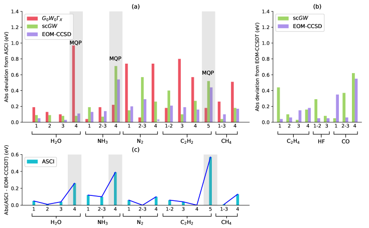
Figure 2: (a) Absolute deviation of sc$GW$, $G_{0}W_{0}\Gamma_{X}$, ⁴⁰ and EOM-CCSD predictions of the first and inner shell ionization peaks as compared with ASCI. Note that bars signified with purple “*” signs meaning that EOM-CCSD calculation did not converge and the deviation is not necessarily zero. Shaded areas are within the MQP regime. (b) Additional molecules calculated with sc$GW$ and EOM-CCSD compared with EOM-CCSDT data. (c) Absolute deviation between ASCI and EOM-CCSDT benchmarks.

In Fig. 2(a), we report IP peaks computed by stochastic $G_{0}W_{0}\Gamma_{X}$, sc$GW$ and EOM-CCSD compared against ASCI data for the 16 excitations from the 5 systems. Out of the total 16 values reported, sc$GW$ yields more accurate data than $G_{0}W_{0}\Gamma_{X}$ for 11 peaks. However, out of the five peaks where $G_{0}W_{0}\Gamma_{X}$ is better than sc$GW$, only for the following three peaks, sc$GW$ is outperformed by $G_{0}W_{0}\Gamma_{X}$ by more than 0.2 eV: the fourth ionization peak of ammonia, the second/third peaks of N₂, and the fifth peak of acetylene. For the IP data in Fig. 2(a), the mean average deviation (MAD) with respect to ASCI for sc$GW$ is 0.21 eV, and for stochastic $G_{0}W_{0}\Gamma_{X}$ is 0.37 eV. Compared with a 1.47 eV MAD given by $G_{0}W_{0}$, both sc$GW$ and $G_{0}W_{0}\Gamma_{X}$ yield inner excitations with much better accuracy.

In addition to the ACSI method, we also compare our results to equation of motion coupled cluster (EOM-CC) ^{78, 79, 80, 81, 82} hierarchy. EOM-CC methods are systematically improvable when adding more excitations and hence here we use EOM-CCSD and EOM-CCSDT values. All EOM-CC calculations were performed using CFOUR ⁸³ quantum chemistry package. Both EOM-CCSD and EOM-CCSDT were performed with aug-cc-pVQZ basis and not extrapolated to the basis set limit. In Fig. 2(c), we look at the difference between inner IPs predicted by EOM-CCSDT and ASCI benchmarks. We observe that the two methods are generally in good agreement with each other (see TABLE. SI in supplemental information for exact numbers). Therefore, EOM-CCSDT could also be used as a benchmark against which $GW$ results can be compared. Although discrepancies between ASCI and EOM-CCSDT tend to increase for deep inner excitations, it remains unclear which of the two methods is more accurate.

Moreover, the comparison allows us to assess the sc$GW$ method against different levels of excitations used in EOM-CC, i.e. EOM-CCSD and EOM-CCSDT. This is helpful for understanding the accuracy that can be expected from sc$GW$ for IP predictions.

In Fig. 2(b), we compare the ionization peaks from sc$GW$ and EOM-CCSD for ethylene (C₂H₄), hydrogen fluoride (HF) and carbon monoxide (CO). For these systems, we employ EOM-CCSDT results in the aug-cc-pVQZ basis-set as reference. Overall, based on the results in panels (a) and (b) of Fig. 2, as well as additional data in Fig. S3 of supplemental information, we deduce that sc$GW$ is similar in accuracy as EOM-CCSD. This similarity is not surprising as connections between $GW$, RPA, and coupled cluster theory have been well studied. ^{84, 85, 86, 87, 88} However, it is worth noticing that EOM-CCSD data were difficult to obtain due to convergence problems for some of the inner peaks while sc$GW$ converged without any difficulty. It is also worth mentioning that for the 4th peaks of H₂O, ammonia and N₂, $G_{0}W_{0}\Gamma_{X}$ gave relatively poor results. For H₂O and N₂, sc$GW$ gave very good results, confirming that the difficulty in illustrating these IPs comes from lack of optimization of orbitals in $G_{0}W_{0}\Gamma_{X}$ and not necessarily from the presence of strong correlation. Only the 4th peak of ammonia displays signs of strong correlation which is not recovered by both sc$GW$ and $G_{0}W_{0}\Gamma_{X}$, and also in EOM-CCSD due to lack of complete convergence.

Further analyzing the results in Fig. 2, the IP data, particularly in panel (a), can be separated into two regimes: (i) single, individual quasiparticle (SQP) and (ii) multi-quasiparticle (MQP). ^{89, 40} For SQPs, the quasiparticle (or the ionization) peak carries most of the spectral weight. Such peaks can be recovered accurately by $GW$ methods. ⁹⁰ On the other hand, for MQP, a significant amount of spectral weight is transferred to satellite features, often referred to as shake-up satellites in molecules. Mean-field and perturbative methods such as DFT and $GW$ are not adept in describing MQPs, as one needs to account for complicated interactions among many excited states.⁴² The general belief is that one can obtain better results for the MQPs by adding higher-order quantum corrections via inclusion of the vertex term, which describes dynamical two-particle correlations.³⁸ However, when looking at the accuracy of the fully self-consistent $GW$ in Fig. 2, we observe that both peaks in the SQP and MQP regimes are well recovered by sc$GW$. Therefore, at least based on the examples considered here, we can confidently say that achieving full self-consistency in $GW$ provides results that are equally, if not more, accurate than vertex-corrected $G_{0}W_{0}$. While both methods provide significant improvements over $G_{0}W_{0}$, one could argue that sc$GW$ is more advantageous over $G_{0}W_{0}\Gamma$ as it provides access to other thermodynamic quantities such as total energy, entropy, etc., in addition to the IP prediction and it is independent of the starting point.

Consequently, at least for the examples listed in Fig. 2(a), the vertex correction seem to be unnecessary and very good results can be obtained by employing sc$GW$ alone. To confirm the points observed above, we plotted spectral functions for selected molecules in the supplemental information (see Fig. S1 and S2). We observe that sc$GW$ also produces similar complicated MQP regime peak structures as reported in Ref. [40]. It further proves that sc$GW$ is capable of depicting the aforementioned shake-up satellites.

IV.2 Comparison of sc$GW$ and $G_{0}W_{0}\Gamma_{0}^{(1)}$ for first IP peaks

Here, we compare the performance of our sc$GW$ to $G_{0}W_{0}\Gamma^{(1)}$ as implemented by Wang et al. and presented in Ref. [31] for the $GW$100 dataset.^{63, 91, 18, 92} This comparison is done only for the first ionization potential peaks, where molecular data sets are more readily available. To ensure that our sc$GW$ data can be compared against the $G_{0}W_{0}\Gamma^{(1)}$ data , we evaluated our sc$GW$ in the same basis set, i.e., def2-TZVPP. For similar reason, for $G_{0}W_{0}$ data, we compare both Hartree-Fock and PBE as mean-field starting points for $GW$ calculations. Further computational details are described in the supplemental information section B.

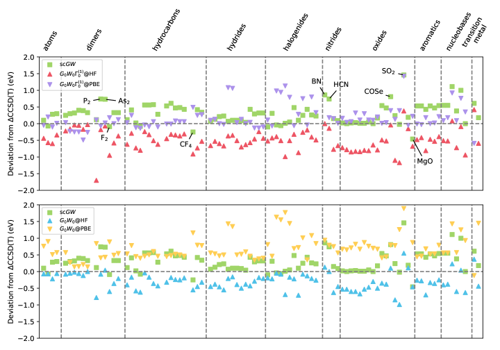
Figure 3: Deviation to $\Delta$CCSD(T) benchmarks, ¹⁸ of $G_{0}W_{0}$, sc$GW$, and $G_{0}W_{0}\Gamma_{0}^{(1)}$ for the $GW$100 data set. Some outliers (within their own group for sc$GW$) are labeled. Top panel: performance of sc$GW$ and $G_{0}W_{0}\Gamma_{0}^{(1)}$ with different starting mean-field calculations. Bottom panel: performance of sc$GW$ and $G_{0}W_{0}$ with different starting mean-field calculations. The data for $G_{0}W_{0}\Gamma_{0}^{(1)}$ where taken from Ref. [31].

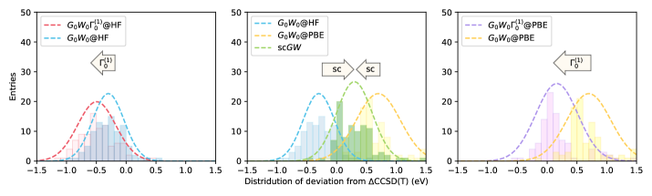
Figure 4: Deviation from $\Delta$CCSD(T) of $G_{0}W_{0}$, sc$GW$, and $G_{0}W_{0}\Gamma_{0}^{(1)}$ for the $GW$100 data set, ^{18, 31} compared with $\Delta$CCSD(T) benchmarks. Dashed lines are fitted Gaussian distributions. Left and right panels: influence of $\Gamma_{0}^{(1)}$ correction on one-shot $GW$ results. Middle panel: improvement introduced by self-consistency upon one-shot $GW$ methodology.

In Fig. 3, we list the first IPs for the $GW$100 molecular data set. In the top panel, we compare the absolute deviations in IPs from sc$GW$ and $G_{0}W_{0}\Gamma_{0}^{(1)}$ based on both PBE and HF starting points. In the bottom panel, we compare IPs for sc$GW$ and $G_{0}W_{0}$ method based on two starting points used in the top panel. All the results are plotted as deviations with respect to $\Delta$CCSD(T) reference values.

By categorizing $GW$100 molecules into ten groups, we observe that sc$GW$ produces low and consistent MAD for hydrides, halogenides, and most oxides. For dimers, hydrocarbons, and aromatics, MAD is higher. For compounds involving bonds with strong polar or ionic character (e.g., CF₄, SO₂, and MgO) sc$GW$ displays larger errors. Unsaturated bonding character (P₂, As₂, BN, HCN) also contributes to abnormal deviations.

In the bottom panel of Fig. 3, we observe that sc$GW$ improves upon one-shot $G_{0}W_{0}$ calculations. While the MAD of $G_{0}W_{0}$@HF is similar to the one of sc$GW$, we see that the majority of deviations for sc$GW$ comes from nucleobases and MgO. In contrast, $G_{0}W_{0}$@PBE displays many outliers for multiple system groups.

In the top panel of Fig. 3, we observe that adding vertex corrections to $G_{0}W_{0}$@HF (denoted as $G_{0}W_{0}\Gamma_{0}^{(1)}$@HF) makes the results consistently worse, while adding vertex correction to $G_{0}W_{0}$@PBE (denoted as $G_{0}W_{0}\Gamma_{0}^{(1)}$@PBE) improves the results making the MAD comparable to sc$GW$.

The peculiar behavior in which different starting points, PBE and HF, change greatly the accuracy of the data when the $\Gamma_{0}^{(1)}$ vertex correction is added on top of $G_{0}W_{0}$ are analyzed in Fig. 4, where we look at the trends in the error distribution curves for $G_{0}W_{0}$, $G_{0}W_{0}\Gamma_{0}^{(1)}$, and sc$GW$. Regardless of the initial starting point used for $G_{0}W_{0}$, the vertex correction $\Gamma_{0}^{(1)}$ systematically enlarges the value of the first IP peak by a similar amount. Because $G_{0}W_{0}$@PBE generally gives smaller IPs than $\Delta$CCSD(T) results, the uniform shift introduced by adding the vertex improves the accuracy of $G_{0}W_{0}\Gamma_{0}^{(1)}$@PBE. For $G_{0}W_{0}$@HF, the IPs are already more accurate than those in $G_{0}W_{0}$@PBE. Consequently, adding vertex correction leads to diminished accuracy. Based on this observation, we argue that the improvement of $\Gamma_{0}^{(1)}$ upon $G_{0}W_{0}$ is serendipitous and the accuracy of the overall result that includes vertex correction is mostly dictated by the starting point dependence. Similar mean-field reference dependence of the vertex corrected results has been observed for IPs of molecules containing transition metals. ⁹³ In sc$GW$, such a starting point dependence is effectively removed via the convergence of a self-consistent loop.

In Table. 1, we present statistical averages for the data presented in Fig. 3. We find that both $G_{0}W_{0}$@HF and $G_{0}W_{0}\Gamma_{0}^{(1)}$@PBE give lower MAD than sc$GW$ when compared with $\Delta$CCSD(T) benchmarks. Even though sc$GW$ does not produce the best MAD out of all cases analyzed, one could still argue that it is more reliable to make predictions with the self-consistent scheme, because even with the pre-existing knowledge about the performance of $G_{0}W_{0}$ on a given system, it will still be difficult to know if $\Gamma_{0}^{(1)}$ would make improvement for such a system.

	$G_{0}W_{0}$	$G_{0}W_{0}\Gamma_{0}^{(1)*}$	sc$GW$
@PBE	0.65($\pm 0.12$)	0.21($\pm 0.09$)	0.33($\pm 0.07$)
@HF	0.33($\pm 0.05$)	0.51($\pm 0.08$)

Table 1: MAD in eV for sc$GW$ and $G_{0}W_{0}$ based on different mean-field starting points for the $GW$100 data set. The fluctuation in the bracket after each MAD value is the variance of absolute deviation. See TABLE. SII (in supplemental information) for detailed IP values for each molecule. ^∗Reported in Ref. ]31].

	$G_{0}W_{0}$	$G_{0}W_{0}\Gamma$	sc$GW$	$\Delta$CCSD(T)∗
cc-pVQZ	0.65($\pm 0.13$)		0.30($\pm 0.07$)	0.23($\pm 0.10$)
cc basis limit	0.88($\pm 0.15$)		0.29($\pm 0.07$)
finite PW∗	0.42($\pm 0.14$)	0.37($\pm 0.10$)
PW basis limit∗	0.69($\pm 0.16$)	0.46($\pm 0.17$)

Table 2: MAD in eV for $GW$ and $\Delta$CCSD(T) methods for the 29-molecule data set, compared with experimental benchmarks. The fluctuation in the bracket after each MAD value is the variance of absolute deviation. See TABLE. SIII (in supplemental information) for detailed IP values for each molecule. ^∗Reported along with the experimental benchmarks for aforementioned data set in Ref. 30.

IV.3 Comparison of sc$GW$ and $G_{0}W_{0}\Gamma$ with non-local vertex corrections for first IP peaks

In Ref. [30], Maggio et al. calculated first IP peaks for 29 molecules using their non-local vertex correction ($G_{0}W_{0}\Gamma$) on top of $G_{0}W_{0}$ in the plane wave (PW) basis. Their final results were extrapolated to the PW basis limit. Here, we compare our sc$GW$ and their $G_{0}W_{0}\Gamma$ for the first IP prediction against the experimental data. ³⁰ Our $G_{0}W_{0}$ and sc$GW$ calculations are performed in the cc-pVXZ (X = Q and 5) basis-sets and then extrapolated to the complete basis-set limit. While we cannot compare these results in a very direct manner since they are performed in different bases, we note that the PW basis and cc basis results behave similarly both in accuracy and basis set convergence trend, when compared against experimental benchmarks. This is also confirmed by Maggio et al. that GTO basis (cc-pVQZ) produced minimal numerical difference (about 100 meV) from finite PW results computed with the same $GW$ implementation. ³⁰

In Tab. 2, for the first IPs, we summarize the overall MAD and variance obtained using $G_{0}W_{0}$ and sc$GW$ and compare it against $G_{0}W_{0}\Gamma$ and $\Delta$CCSD(T) results from Ref. [30]. Corresponding numerical data is presented in Table SIII of SI. We observe that by extrapolating $G_{0}W_{0}$ and $G_{0}W_{0}\Gamma$ results from a finite bases to their respective limits, the accuracy deteriorates even though higher number of orbitals are included. For cc basis-sets, the MAD for our $G_{0}W_{0}$ increases from 0.65 eV (cc-pVQZ) to 0.88 eV (cc basis limit). Similarly, for the results in plane wave basis (adopted from Ref. [30]), the MAD of $G_{0}W_{0}$ increases from 0.42 eV (finite plane wave) to 0.69 eV (plane wave basis limit), and the MAD of $G_{0}W_{0}\Gamma$ increases from 0.37 eV (finite plane wave) to 0.69 eV (plane wave basis limit). In Ref. [30], the phenomenon was also coupled with convergence issue for some molecules (lithium dimer, phosphorus dimer, and sulfur dioxide) for $G_{0}W_{0}\Gamma$ extrapolation results with PW basis set. On the other hand sc$GW$ results are fairly converged already at the cc-pVQZ level.

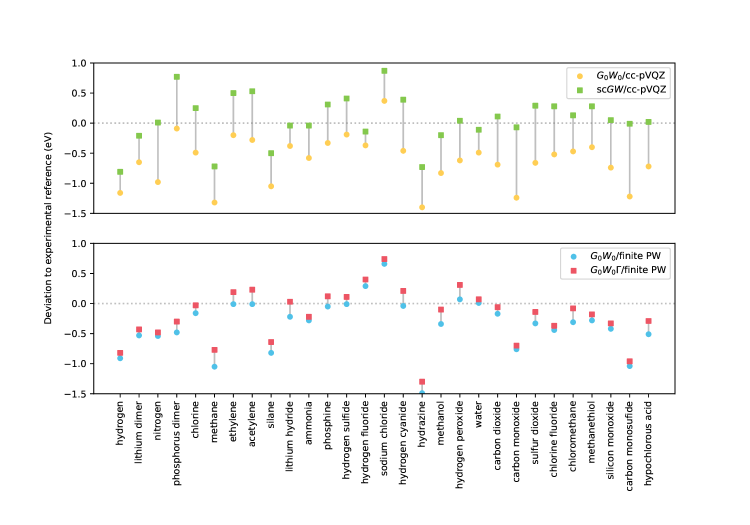
Figure 5: Deviation with respect to experimental data of $G_{0}W_{0}$, sc$GW$, and $G_{0}W_{0}\Gamma$ for the 29-molecule data set. Top panel: improvement brought upon $G_{0}W_{0}$ prediction by self-consistency in a finite cc basis. Bottom panel: improvement brought by including vertex correction on top of $G_{0}W_{0}$ in a finite plane wave basis. ³⁰

Table 2 shows that in the CBS limit for plane waves, vertex correction reduces the MAD for the IPs from 0.69 eV in $G_{0}W_{0}$ to 0.46 eV. Meanwhile, in the CBS limit for cc-basis-set family, the self-consistency improves the MAD from 0.88 eV at the $G_{0}W_{0}$ level to 0.29 eV for sc$GW$.

The magnitude of improvement induced by both self-consistency and vertex correction is illustrated in Fig. 5. In the top panel of Fig. 5, we observe that performing self-consistency in most cases brings the IP values closer to experiment in comparison to $G_{0}W_{0}$. The bottom panel shows the magnitude of the improvement brought by vertex correction on top of $G_{0}W_{0}$, which is only minor. Thus, its final accuracy largely depends on a good mean-field starting pointing point of the $G_{0}W_{0}$ calculations.

Overall, we conclude that in the molecular IP domain, improvements introduced by self-consistency is similar to, if not better than, that of vertex corrected $G_{0}W_{0}$. Moreover, the significantly smaller variance in sc$GW$ (0.07 eV vs. 0.17 eV in $G_{0}W_{0}\Gamma$) implies more uniformity in the quality of results. This, combined with the lack of dependence on the starting mean-field solution, makes sc$GW$ more favorable.

V Conclusion

In this work, we demonstrated the performance of finite temperature (imaginary axis) sc$GW$ methodology in predicting molecular valence shell IPs. In our implementation, there are no approximations other than a) density fitting approximation for integral generation; and b) the Nevanlinna analytical continuation employed to obtain spectral data from the converged Green’s function evaluated on the imaginary axis.

Based on our calculations, performing the self-consistency generally improves upon $G_{0}W_{0}$ results (or maintains a similar level of accuracy) and leads to convergence of calculations with different mean-field starting points to the same result. This eliminates the ambiguity associated with the selection of a mean-field calculation used as the reference for the GW method. The reliability of our sc$GW$ method is verified both for the first IPs as well for the inner valence shell IPs, when examined against theoretical and experimental results.

For molecular systems, we presented comparisons of our sc$GW$ with another post-$GW$ methodology – vertex corrected $G_{0}W_{0}$ – motivated by considering the complete suite of Hedin’s equations. When comparing different $G_{0}W_{0}\Gamma$ variants against sc$GW$, we observed that sc$GW$ consistently displays either better or comparable accuracy. The $G_{0}W_{0}\Gamma$ results are affected by a strong starting point dependence (inherited from $G_{0}W_{0}$ starting point) and the magnitude of deviation due the starting point is frequently larger than the correction introduced by the vertex. Similar dependence was also observed in vertex correction upon polarizability. ⁹⁴

Even though there are scattered cases where $G_{0}W_{0}\Gamma$ based on a particular DFT reference outperforms sc$GW$, performing full self-consistency is cheaper than evaluating full vertex corrections and gives unbiased results independent of the starting point. Moreover, within the sc$GW$ framework, the evaluation of total energies and, consequently, energy differences is possible. ^{95, 96, 97, 35}

Additionally, choosing appropriate type of vertex correction can be a difficult task. In this work, we analyzed three different versions of vertex corrections each employing different approximations and we concluded that it is hard to establish a priori which type of vertex correction should be used.

While sc$GW$ is generally accurate for first IP as well as inner valence-shell excitations, depiction of excitations with multi-quasiparticle-peak (MQP) character might be relatively difficult. In MQPs, due to correlation effects, the spectral weight from the primary quasiparticle excitations is transferred to satellite features. Nevertheless, for the examples analyzed in Sec. IV.1, it appears that sc$GW$ is capable of not only capturing the qualitative emergence of satellites, but also yields reasonably accurate quasiparticle energies for the MQPs. This is particularly advantageous in comparison to methods such as EOM-CCSD, where the presence of satellites may lead to issues with converging the quasiparticle energies.

Vertex correction is generally considered as a preferred way to improve the quality of $G_{0}W_{0}$ results. However, we find that at least for molecules, sc$GW$, without vertex, already provides results that are competitive with the best $G_{0}W_{0}\Gamma$ results. This, combined with the fact that sc$GW$ is essentially a black-box method, makes self-consistency a better route to make improvements upon $G_{0}W_{0}$. We argue that the implementation of vertex correction should be done based on the self-consistent sc$GW$ approach where the starting point dependence is removed. Only then the approximations introduced in the formulation of $GW\Gamma$ can be meaningfully validated. When starting from sc$GW$, the vertex correction is responsible only for bringing the correlation that is missing in the parent sc$GW$ approach, it does not need to remedy for the lack of the orbital optimization that is present in $G_{0}W_{0}$. This direction will be explored in our future work.

Supplemental Information

A. Inner valence shell ionizations

In TABLE SI, we report our detailed data for the first and few inner valence ionization peaks for each molecule entry. For ammonia, water, nitrogen, acetylene, and methane, $G_{0}W_{0}\Gamma_{X}$ and ASCI results were reported by Mejuto-Zaera et. al. ⁴⁰ The EOM columns refer to EOM-CCSDT/aug-cc-pVQZ method.

Molecule	Peak	$G_{0}W_{0}\Gamma_{X}$	sc$GW$	EOM-CCSD	EOM-CCSDT	ASCI
Ethylene	1		-10.28	-10.76	-10.72
	2		-13.20	-13.16	-13.10
	3		-14.83	-15.01	-14.86
	4		-16.36	-16.38	-16.20
Hydrogen fluoride	1-2		-16.39	-16.15	-16.10
	3		-20.09	-20.06	-20.01
	4		-39.57	**	**
Carbon monoxide	1		-14.20	-14.50	-14.15
	2-3		-15.20	-15.63	-15.57
	4		-19.64	-19.57	-19.02
	5		-33.57	**	**
Ammonia	1	-10.85	-11.00	-10.94	-10.93	-10.81
	2-3	-16.70	-16.58	-16.65	-16.61	-16.51
	4	-27.58	-28.07	-27.90	-26.97	-27.36
Water	1	-12.94	-12.84	-12.70	-12.70	-12.75
	2	-15.03	-14.99	-14.90	-14.91	-14.90
	3	-19.20	-19.02	-19.07	-19.06	-19.10
	4	-32.02	-32.91	-32.88	-32.73	-32.99
Nitrogen	1	-16.28	-15.69	-15.74	-15.60	-15.54
	2-3	-17.11	-16.48	-17.34	-17.05	-17.05
	4	-19.62	-19.14	**	-18.98	-18.88
Acetylene	1-2	-11.27	-11.05	-11.66	-11.51	-11.45
	3	-17.95	-17.25	-17.34	-17.19	-17.15
	4	-19.62	-19.32	-19.21	-19.05	-19.05
	5	-24.31	-24.65	-24.57	-24.70	-24.13
Methane*	1-3	-14.61	-14.39	-14.45	-14.36	-14.35
	4	-22.74	-23.43	-23.42	-23.12	-23.25

Table SI: First few ionization potentials (in eV) for molecules. ^∗Methane’s $G_{0}W_{0}\Gamma$ and ASCI results were reported in cc basis. ^∗∗Unable to converge.

In FIG. S1 and S2, we present three examples of spectral functions produced from the same sc$GW$ calculations via Nevanlinna analytical continuation. Similar spectral functions rendered by stochastic $G_{0}W_{0}\Gamma_{X}$ are reported in Ref. ⁴⁰. Notice that in ammonia and water we have the complicated multi-peak feature in the MQP regime. We identify the MQP peak by increasing the broadening factor so that the complicated multi-peak feature melts into a singular broad peak, which corresponds to the number we report in TABLE SI.

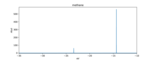
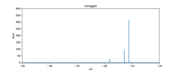
Figure S1: Spectral functions of methane and nitrogen.

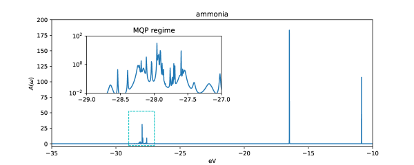
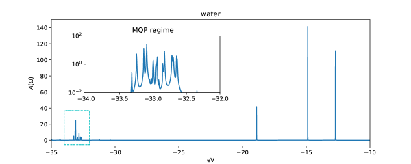
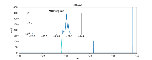
Figure S2: Spectral functions of ammonia, water, and acetylene. The MQP regimes insets are plotted in alogarithmic scale.

In FIG. S3, we present the absolute deviation when swapping the EOM-CCSDT benchmarks (in the main text) to the ASCI benchmarks reported by by Mejuto-Zaera et. al. ⁴⁰

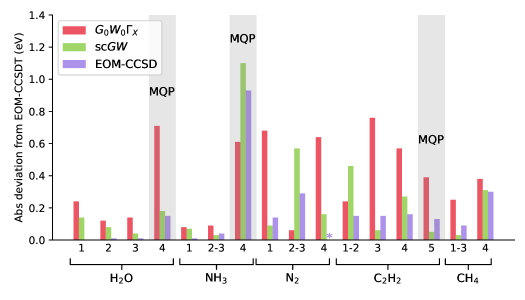
Figure S3: Absolute deviation of sc$GW$, $G_{0}W_{0}\Gamma_{X}$, and EOM-CCSD predictions of the first and inner shell ionization peaks from the EOM-CCSDT data. ^∗Some EOM-CCSD calculation did not converge.

B. First ionization peaks

We present our test on the $GW$100 set. We compare our sc$GW$ method to $G_{0}W_{0}\Gamma_{0}^{(1)}$ by Wang et al. ³¹ while keeping the level of theory as similar as possible. Initializations for both approaches are done using PBE/def2-TZVPP. Molecules containing elements in the fourth row or beyond are excluded, since the all-electron basis set of def2-TZVPP for these elements is not available. Total of 93 molecules are kept.

Firstly, we need to confirm that finite temperature sc$GW$ (on the imaginary axis) and $G_{0}W_{0}\Gamma_{0}^{(1)}$ by Wang et al. (on the real axis) can produce the same results after the first iteration, i.e. the $G_{0}W_{0}$ level. If so, we can make sure the comparison is appropriate and and based on similar theoretical footing. In FIG. S4 the $G_{0}W_{0}$ results for both schemes fit well with no obvious outliers, giving a 0.05 eV MAD. This observation also supports that one can recover spectral information from the Green’s function on imaginary axis via analytical continuation, which is directly available on the real axis.

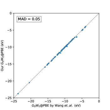
Figure S4: Comparison of ionization potentials derived from Rinke’s $G_{0}W_{0}$@PBE and our finite temperature version of $G_{0}W_{0}$@PBE.

Index	Molecule	$G_{0}W_{0}$@HF	$G_{0}W_{0}$@PBE	sc$GW$	CCSD(T)∗		Index	Molecule	$G_{0}W_{0}$@HF	$G_{0}W_{0}$@PBE	sc$GW$	CCSD(T)∗
1	He	-24.58	-23.75	-24.41	-24.51		53	HCl	-12.81	-12.13	-12.28	-12.59
2	Ne	-21.39	-20.49	-21.39	-21.32		54	LiF	-11.37	-9.77	-11.36	-11.32
3	Ar	-15.76	-15.02	-15.26	-15.54		55	MgF2	-13.79	-12.29	-13.77	-13.71
4	Kr	-14.00	-13.37	-13.64	-13.94		56	TiF4	-16.17	-13.77	-15.47	-15.48
6	H2	-16.48	-15.90	-16.15	-16.40		57	AlF3	-15.63	-14.14	-15.41	-15.46
7	Li2	-5.32	-5.05	-4.97	-5.27		58	BF	-11.31	-10.43	-10.61	-11.09
8	Na2	-4.97	-4.92	-4.63	-4.95		59	SF4	-13.30	-11.91	-12.49	-12.59
9	Na4	-4.29	-4.11	-3.83	-4.23		60	KBr	-8.21	-7.15	-7.88	-8.13
10	Na6	-4.47	-4.25	-3.96	-4.35		61	GaCl	-9.90	-9.42	-9.34	-9.77
11	K2	-4.06	-3.94	-3.73	-4.06		62	NaCl	-9.24	-7.90	-8.77	-9.03
13	N2	-16.35	-14.74	-15.45	-15.57		63	MgCl2	-11.93	-10.84	-11.44	-11.67
14	P2	-10.55	-10.05	-9.73	-10.47		65	BN	-11.76	-11.08	-11.03	-11.89
15	Ar2	-9.74	-9.34	-9.05	-9.78		66	HCN	-13.87	-13.00	-13.13	-13.87
16	F2	-16.31	-14.83	-15.80	-15.71		67	PN	-12.37	-10.99	-11.59	-11.74
17	Cl2	-11.77	-10.90	-11.08	-11.41		68	N2H4	-10.17	-9.21	-9.63	-9.72
18	Br2	-10.75	-9.98	-10.21	-10.54		69	CH2O	-11.37	-10.17	-10.82	-10.84
20	CH4	-14.77	-13.91	-14.25	-14.37		70	CH3OH	-11.57	-10.46	-11.04	-11.04
21	C2H6	-13.21	-12.35	-12.63	-13.04		71	EtOH	-11.29	-10.05	-10.67	-10.69
22	C3H8	-12.63	-11.66	-12.03	-12.05		72	CH3CHO	-10.81	-9.40	-10.18	-10.21
23	C4H${}_{1}0$	-12.19	-11.23	-11.65	-11.57		73	Et2O	-10.49	-9.21	-9.81	-9.82
24	C2H4	-10.71	-10.20	-10.11	-10.67		74	HCOOH	-11.95	-10.59	-11.41	-11.42
25	C2H2	-11.59	-10.94	-10.86	-11.42		75	H2O2	-12.06	-10.87	-11.54	-11.59
26	C4	-11.62	-10.64	-10.69	-11.26		76	water	-12.87	-11.94	-12.57	-12.57
27	C2H6	-11.30	-10.46	-10.59	-10.87		77	CO2	-14.21	-13.07	-13.54	-13.71
28	C6H6	-9.52	-8.87	-8.75	-9.29		78	CS2	-10.33	-9.55	-9.44	-9.98
29	C8H8	-8.67	-7.93	-7.82	-8.35		79	OCS	-11.55	-10.74	-10.70	-11.17
30	C5H6	-8.86	-8.23	-8.07	-8.68		80	COSe	-10.69	-10.00	-9.98	-10.79
31	C2H3F	-10.79	-10.02	-10.08	-10.55		81	CO	-15.06	-13.43	-13.97	-14.21
32	C2H3Cl	-10.34	-9.58	-9.61	-10.09		82	O3	-13.54	-11.73	-12.57	-12.55
33	C2H3Br	-9.46	-8.83	-8.84	-9.27		83	SO2	-12.94	-11.61	-12.03	-13.49
35	CF4	-16.85	-15.18	-16.55	-16.30		84	BeO	-9.83	-9.16	-9.75	-9.94
36	CCl4	-12.01	-10.77	-11.14	-11.56		85	MgO	-7.95	-7.05	-7.95	-7.49
37	CBr4	-10.78	-9.67	-10.12	-10.46		86	C6H5CH3	-9.16	-8.49	-8.37	-8.90
39	SiH4	-13.25	-12.28	-12.73	-12.80		87	C6H5Et	-9.13	-8.43	-8.32	-8.85
40	GeH4	-12.88	-11.99	-12.37	-12.50		88	C6F6	-10.63	-9.28	-9.50	-9.93
41	Si2H6	-11.11	-10.21	-10.44	-10.65		89	C6H5OH	-9.03	-8.22	-8.17	-8.70
42	Si5H${}_{1}2$	-9.82	-8.81	-9.04	-9.27		90	C6H5NH2	-8.35	-7.49	-7.52	-7.99
43	LiH	-8.17	-7.02	-7.89	-7.96		91	C5H5N	-9.91	-8.87	-9.12	-9.66
44	KH	-6.29	-4.81	-6.03	-6.13		92	guanine	-8.44	-7.52	-7.48	-8.03
45	BH3	-13.67	-12.84	-13.18	-13.28		93	adenine	-8.71	-7.80	-7.78	-8.33
46	B2H6	-12.76	-11.74	-12.17	-12.26		94	cytosine	-9.28	-8.08	-8.40	-9.51
47	NH3	-11.19	-10.29	-10.77	-10.81		95	thymine	-9.68	-8.49	-8.70	-9.08
48	HN3	-11.11	-10.27	-10.25	-10.68		96	uracil	-10.09	-8.86	-9.13	-10.13
49	PH3	-10.81	-10.20	-10.23	-10.52		97	urea	-10.68	-9.18	-10.05	-10.05
50	ArH3	-10.58	-10.04	-10.08	-10.40		99	Cu2	-7.20	-7.61	-6.96	-7.57
51	H2S	-10.52	-9.92	-9.99	-10.31		100	CuCN	-11.29	-9.80	-10.67	-10.85
52	HF	-16.22	-15.29	-16.13	-16.03			MAD	0.33	0.65	0.33

Table SII: First ionization potentials (in eV) calculated from $G_{0}W_{0}$@PBE, sc$GW$, and $\Delta$CCSD(T) for the $GW$100 set. ^∗Reported in Ref. ³¹.

We use HF/cc-pVXZ (X = Q and 5) as the starting point for our subsequent scGW calculations for the 29-molecule data set. Then we compare these results with the vertexed corrected $G_{0}W_{0}$ method propesed by Maggio et. al. ³⁰ Final sc$GW$ results are linearly extrapolated to cc basis set limit. The cited data calculated in the plane wave basis were also evaluated with HF starting mean field. Please refer to the original article for their detailed description for energy cut-offs and the extrapolation technique for the PW basis.

	cc-pVQZ				cc basis limit			finite PW∗			PW basis limit∗
Molecule	CCSD(T)∗	$G_{0}W_{0}$	sc$GW$		$G_{0}W_{0}$	sc$GW$		$G_{0}W_{0}$	$G_{0}W_{0}\Gamma$		$G_{0}W_{0}$	$G_{0}W_{0}\Gamma$	Experiment∗
hydrogen	-16.39	-16.59	-16.24		-16.65	-16.32		-16.34	-16.25		-16.72	-16.52	-15.43
lithium dimer	-5.17	-5.38	-4.94		-5.42	-4.94		-5.26	-5.16		-5.29		-4.73
nitrogen	-15.49	-16.56	-15.57		-16.82	-15.66		-16.12	-16.06		-16.56	-16.39	-15.58
phosphorus dimer	-10.76	-10.71	-9.85		-11.01	-9.98		-11.10	-10.92		-11.31		-10.62
chlorine	-11.62	-11.98	-11.24		-12.35	-11.37		-11.65	-11.52		-12.08	-11.80	-11.49
methane	-14.40	-14.92	-14.32		-15.05	-14.37		-14.65	-14.37		-14.95	-14.57	-13.6
ethylene	-10.69	-10.88	-10.18		-11.04	-10.24		-10.69	-10.49		-10.91	-10.66	-10.68
acetylene	-11.42	-11.77	-10.96		-11.95	-11.13		-11.50	-11.26		-11.73	-11.43	-11.49
silane	-12.82	-13.35	-12.80		-13.50	-12.89		-13.12	-12.94		-13.40	-12.88	-12.3
lithium hydride	-7.94	-8.28	-7.94		-8.39	-8.02		-8.12	-7.87		-8.26	-7.94	-7.90
ammonia	-10.92	-11.40	-10.86		-11.60	-10.98		-11.10	-11.04		-11.45	-11.28	-10.82
phosphine	-10.49	-10.92	-10.28		-11.14	-10.48		-10.64	-10.47		-10.89	-10.66	-10.59
hydrogen sulfide	-10.43	-10.69	-10.09		-10.97	-10.15		-10.51	-10.39		-10.79	-10.60	-10.50
hydrogen fluoride	-16.09	-16.49	-16.26		-16.79	-16.41		-15.83	-15.72		-16.29	-16.18	-16.12
sodium chloride	-9.13	-9.43	-8.93		-9.83	-9.09		-9.14	-9.06		-9.51	-9.32	-9.80
hydrogen cyanide	-13.64	-14.07	-13.22		-14.28	-13.44		-13.65	-13.4		-13.92	-13.61	-13.61
hydrazine	-10.24	-10.38	-9.71		-10.61	-9.83		-10.47	-10.28		-10.86	-10.58	-8.98
methanol	-11.08	-11.79	-11.16		-12.03	-11.33		-11.30	-11.06		-11.71	-11.39	-10.96
hydrogen peroxide	-11.49	-12.32	-11.66		-12.62	-11.91		-11.63	-11.39		-12.12	-11.81	-11.70
water	-12.64	-13.11	-12.73		-13.38	-12.80		-12.61	-12.55		-13.10	-12.92	-12.62
carbon dioxide	-13.78	-14.46	-13.66		-14.78	-13.92		-13.94	-13.83		-14.35	-14.16	-13.77
carbon monoxide	-14.05	-15.25	-14.08		-15.47	-14.17		-14.77	-14.71		-15.03	-14.89	-14.01
sulfur dioxide	-12.41	-13.16	-12.21		-13.60	-12.48		-12.83	-12.64		-13.20		-12.50
chlorine fluoride	-12.82	-13.29	-12.49		-13.67	-12.73		-13.21	-13.14		-13.49	-13.33	-12.77
chloromethane	-11.41	-11.76	-11.16		-12.10	-11.24		-11.60	-11.37		-11.90	-11.56	-11.29
methanethiol	-9.49	-9.84	-9.16		-10.12	-9.35		-9.72	-9.62		-9.93	-9.76	-9.44
silicon monoxide	-11.55	-12.04	-11.25		-12.30	-11.35		-11.72	-11.63		-12.05	-11.78	-11.3
carbon monosufide	-11.45	-12.55	-11.34		-12.80	-11.44		-12.37	-12.29		-12.63	-12.47	-11.33
hypochlorous acid	-11.30	-11.84	-11.10		-12.20	-11.30		-11.63	-11.41		-11.96	-11.66	-11.12
MAD from experiment	0.23	0.65	0.30		0.88	0.29		0.42	0.37		0.69	0.46

Table SIII: First ionization potentials (in eV) calculated from CCSD(T), $G_{0}W_{0}$@HF, sc$GW$, and $G_{0}W_{0}\Gamma$@HF, in cc basis and plane wave basis. ^∗Reported in Ref. ³⁰.