Sensitivity of polarizations and spin correlations of Zš‘Z boson to anomalous
neutral triple gauge couplings at lepton collider with polarized beams

Amir Subba as19rs008@iiserkol.ac.in ā€ƒā€ƒ Ritesh K. Singh ritesh.singh@iiserkol.ac.in Department of Physical Sciences, Indian Institute of Science Education and Research Kolkata, Mohanpur, 741246, India
Abstract

We investigate the effects of anomalous neutral triple gauge couplings in Zā€‹Zš‘š‘ZZ and Zā€‹Ī³š‘š›¾Z\gamma production processes, followed by the leptonic decay of the Zš‘Z boson, at a lepton collider with center-of-mass energy s=250š‘ 250\sqrt{s}=250 GeV and polarized beams. We use an effective Lagrangian formalism to parameterize the anomalous couplings in terms of dimension-8 operators cB~ā€‹Wsubscriptš‘~šµš‘Šc_{\widetilde{B}W}, cBā€‹Wsubscriptš‘šµš‘Šc_{BW}, cWā€‹Wsubscriptš‘š‘Šš‘Šc_{WW}, and cBā€‹Bsubscriptš‘šµšµc_{BB}, and study the sensitivity of observables such as crossĀ section, polarization, and spin correlation as functions of these couplings. We perform a Bayesian statistical analysis using Markov Chain Monte Carlo methods to determine simultaneous limits on the anomalous couplings, taking into account various luminosities ā„’āˆˆ{0.1ā€‹abāˆ’1,0.3ā€‹abāˆ’1,1ā€‹abāˆ’1,3ā€‹abāˆ’1,10ā€‹abāˆ’1}ā„’0.1superscriptab10.3superscriptab11superscriptab13superscriptab110superscriptab1\mathcal{L}\in\{0.1~{}\text{ab}^{-1},0.3~{}\text{ab}^{-1},1~{}\text{ab}^{-1},3~{}\text{ab}^{-1},10~{}\text{ab}^{-1}\} and systematic uncertainties. We find that polarization and spin correlation observables significantly enhance the sensitivity to anomalous couplings, providing stringent constraints on these couplings.

ā€ ā€ preprint: APS/123-QED

I Introduction

The Standard ModelĀ (SM) of particle physics is a marvel of scientific achievement. It has undergone rigorous experimental scrutiny to emerge as the most extensively tested theory of fundamental particles and their interactions. The discovery of scalar JP=0+superscriptš½š‘ƒsuperscript0J^{P}=0^{+} boson by ATLASĀ [1] and CMSĀ [2] collaborations at LHC consistent with the Standard Model Higgs boson completes the particle spectrum of SM. However, some unresolved issues exist within the SM framework, including fine-tuning the Higgs boson mass, which is susceptible to higher-order quantum corrections that could shift the mass away from the experimental value of 125 GeV. Another unresolved issue is the strong-CP problem, which refers to the unexplained value of the theta parameter (Īøšœƒ\theta) in the quantum chromodynamics (QCD) sector of the SM. Furthermore, dark matterĀ [3], which constitutes approximately 85%percent8585\% of the matter in the Universe, remains a mystery, and its structure still needs to be fully understood. Explaining the non-zero mass of neutrinos and the transformation between the three generations of neutrinos requires physics beyond SM. Recent measurements of the Wš‘ŠW boson massĀ [4] and the magnetic moment of the muonĀ [5] have shown significant deviations from the SM. Several models have been proposed to address these shortcomings, such as supersymmetry, technicolor, universal extra dimensions, and string theory, which incorporate extra dimensions, new symmetries, and new particles. However, no experimental evidence has yet confirmed any of these models.

In the absence of any signature in favor of specific models, one adopts a model-independent framework to parameterize the effects beyond the Standard Model, known as the effective field theoryĀ (EFT)Ā [6, 7, 8] approach. This approach extends the SM Lagrangian by adding higher-order gauge invariant terms constructed from SM states. In general, if a field theory contains a set of fields Aš“A and BšµB, where Aš“A is light, and BšµB are heavy states, then the action š’®~ā€‹[A]~š’®delimited-[]š“\widetilde{\mathcal{S}}\left[A\right] of the effective field theory may be obtained from the action š’®ā€‹[A,B]š’®š“šµ\mathcal{S}\left[A,B\right] of the full field theory by a functional integral over BšµB, e(iā€‹š’®~ā€‹[A])=āˆ«[dā€‹B]ā€‹eiā€‹š’®ā€‹[A,B]superscriptš‘’š‘–~š’®delimited-[]š“delimited-[]dšµsuperscriptš‘’š‘–š’®š“šµe^{\left(i\widetilde{\mathcal{S}}\left[A\right]\right)}=\int\left[\text{d}B\right]e^{i\mathcal{S}\left[A,B\right]}. One of the issues with this indirect formalism is the possibility of matching low energy theory to multiple UV complete theory. Such ambiguities are removed only with the discovery of new particles. Usually, the EFT approach remains valid upto some characteristic energy scale, Ī›Ī›\Lambda, such that Ī›>MEWĪ›subscriptš‘€EW\Lambda>M_{\text{EW}}, MEWsubscriptš‘€EWM_{\text{EW}} is the electroweak scale. Each higher dimensional termsĀ (d>4š‘‘4d>4) are weighted by Ī›dāˆ’4superscriptĪ›š‘‘4\Lambda^{d-4} power, such that the effective Lagrangian is,

ā„’eff=ā„’SM+1Ī›2ā€‹āˆ‘ici(6)ā€‹š’Ŗi(6)+1Ī›4ā€‹āˆ‘ici(8)ā€‹š’Ŗi(8)+..,subscriptā„’effsubscriptā„’SM1superscriptĪ›2subscriptš‘–superscriptsubscriptš‘š‘–6superscriptsubscriptš’Ŗš‘–6limit-from1superscriptĪ›4subscriptš‘–superscriptsubscriptš‘š‘–8superscriptsubscriptš’Ŗš‘–8\mathscr{L}_{\text{eff}}=\mathscr{L}_{\text{SM}}+\frac{1}{\Lambda^{2}}\sum_{i}c_{i}^{(6)}\mathscr{O}_{i}^{(6)}+\frac{1}{\Lambda^{4}}\sum_{i}c_{i}^{(8)}\mathscr{O}_{i}^{(8)}+.., (1)

where the sum over iš‘–i runs over a basis {š’Ŗi(d)}superscriptsubscriptš’Ŗš‘–š‘‘\{\mathscr{O}_{i}^{(d)}\} in the dāˆˆ{6,8,10,..}d\in\{6,8,10,..\}-dimension gauge-invariant operator space and cā€²ā€‹ssuperscriptš‘ā€²š‘ c^{\prime}s are Wilson coefficients related to those operators. Since the scale of new physics is in several TeV, the higher order terms are highly suppressed; thus, we can safely truncate the expansion in Eq.Ā (1) to some lowest order for collider energy of few TeVs. The presence of these operators affects various structures like couplings of bosons and fermions, and the vacuum expectation value of the Higgs field. The deviation in these structures can be experimentally probed through measurements of various observables.

The SM non-abelian Sā€‹Uā€‹(2)ƗUā€‹(1)š‘†š‘ˆ2š‘ˆ1SU(2)\times U(1) gauge structure induces triple and quartic gauge boson couplings. Studies of triple and quartic couplings between the gauge bosons test the SM description of gauge sector interactions and provide sensitivity to physics beyond the SM by examining production rates and kinematics. In the case of triple gauge couplings, the structure SM allows is Wāˆ’ā€‹W+ā€‹V,Vāˆˆ{Ī³,Z}superscriptš‘Šsuperscriptš‘Šš‘‰š‘‰š›¾š‘W^{-}W^{+}V,~{}V\in\{\gamma,Z\}, and no neutral triple gauge couplingsĀ (NTGC) at tree level. At the lowest order, such charged triple gauge boson couplings are affected by dimension-6 operators, while NTGC is generated by dimension-8 operatorsĀ [9] at the tree level. Besides operator formalism, anomalous NTGCĀ (aNTGC) can also be parameterized as effective vertex. Assuming only Lorentz and Uā€‹(1)emš‘ˆsubscript1emU(1)_{\text{em}} gauge invariance, the most general V1ā€‹V2ā€‹V3subscriptš‘‰1subscriptš‘‰2subscriptš‘‰3V_{1}V_{2}V_{3} vertex function, where V2,3subscriptš‘‰23V_{2,3} are on-shell neutral gauge bosons, while V1āˆˆ{Zā‹†,Ī³ā‹†}subscriptš‘‰1superscriptš‘ā‹†superscriptš›¾ā‹†V_{1}\in\{Z^{\star},\gamma^{\star}\} is off-shell, can be written asĀ [10, 11],

iā€‹eā€‹Ī“Vā€‹Zā€‹ZĪ±ā€‹Ī²ā€‹Ī³ā€‹(q1,q2,q3)š‘–š‘’subscriptsuperscriptĪ“š›¼š›½š›¾š‘‰š‘š‘subscriptš‘ž1subscriptš‘ž2subscriptš‘ž3\displaystyle ie\Gamma^{\alpha\beta\gamma}_{VZZ}(q_{1},q_{2},q_{3}) =āˆ’eā€‹(q12āˆ’mV2)mZ2[f4V(q1Ī±gĪ¼ā€‹Ī²+q1Ī²gĪ¼ā€‹Ī±)\displaystyle=\frac{-e(q_{1}^{2}-m_{V}^{2})}{m_{Z}^{2}}\left[f_{4}^{V}\left(q_{1}^{\alpha}g^{\mu\beta}+q_{1}\beta g^{\mu\alpha}\right)\right. (2)
āˆ’f5VĻµĪ¼ā€‹Ī±ā€‹Ī²ā€‹Ļ(q2āˆ’q3)Ļ],\displaystyle-\left.f_{5}^{V}\epsilon^{\mu\alpha\beta\rho}\left(q_{2}-q_{3}\right)_{\rho}\right],
iā€‹eā€‹Ī“Vā€‹Zā€‹Ī³Ī±ā€‹Ī²ā€‹Ī¼ā€‹(q1,q2,q3)š‘–š‘’subscriptsuperscriptĪ“š›¼š›½šœ‡š‘‰š‘š›¾subscriptš‘ž1subscriptš‘ž2subscriptš‘ž3\displaystyle ie\Gamma^{\alpha\beta\mu}_{VZ\gamma}(q_{1},q_{2},q_{3}) =āˆ’eā€‹(q12āˆ’mV2)mZ2[h1V(q3VgĪ±ā€‹Ī²āˆ’q3Ī±gĪ¼ā€‹Ī²)\displaystyle=\frac{-e(q_{1}^{2}-m_{V}^{2})}{m_{Z}^{2}}\left[h_{1}^{V}\left(q_{3}^{V}g^{\alpha\beta}-q_{3}^{\alpha}g^{\mu\beta}\right)\right.
+h2VmZ2ā€‹q1Ī±ā€‹(q1ā€‹q3ā€‹gĪ¼ā€‹Ī²āˆ’q3Ī¼ā€‹q1Ī²)superscriptsubscriptā„Ž2š‘‰superscriptsubscriptš‘šš‘2superscriptsubscriptš‘ž1š›¼subscriptš‘ž1subscriptš‘ž3superscriptš‘”šœ‡š›½subscriptsuperscriptš‘žšœ‡3subscriptsuperscriptš‘žš›½1\displaystyle+\left.\frac{h_{2}^{V}}{m_{Z}^{2}}q_{1}^{\alpha}\left(q_{1}q_{3}g^{\mu\beta}-q^{\mu}_{3}q^{\beta}_{1}\right)\right.
āˆ’h3VĻµĪ¼ā€‹Ī±ā€‹Ī²ā€‹Ļq3ā€‹Ļāˆ’h4VmZ2q1VĻµĪ¼ā€‹Ī²ā€‹Ļā€‹Ļƒq1ā€‹Ļq3ā€‹Ļƒ],\displaystyle-\left.h_{3}^{V}\epsilon^{\mu\alpha\beta\rho}q_{3\rho}-\frac{h_{4}^{V}}{m_{Z}^{2}}q_{1}^{V}\epsilon^{\mu\beta\rho\sigma}q_{1\rho}q_{3\sigma}\right],

where Vāˆˆ{Z,Ī³}š‘‰š‘š›¾V\in\{Z,\gamma\}. The effective Lagrangian generating the above two vertices is,

ā„’ā„’\displaystyle\mathscr{L} =emZ2[āˆ’[f4Ī³(āˆ‚Ī¼FĪ¼ā€‹Ī²)+f4Z(āˆ‚Ī¼ZĪ¼ā€‹Ī²)]ZĪ±(āˆ‚Ī±ZĪ²)+[f5Ī³(āˆ‚ĻƒFĻƒā€‹Ī¼)+f5Z(āˆ‚ĻƒZĻƒā€‹Ī¼)]Z~Ī¼ā€‹Ī²ZĪ²āˆ’[h1Ī³(āˆ‚ĻƒFĻƒā€‹Ī¼)+h1Z(āˆ‚ĻƒZĻƒā€‹Ī¼)]ZĪ²FĪ¼ā€‹Ī²\displaystyle=\frac{e}{m_{Z}^{2}}\left[-[f_{4}^{\gamma}(\partial_{\mu}F^{\mu\beta})+f_{4}^{Z}(\partial_{\mu}Z^{\mu\beta})]Z_{\alpha}(\partial^{\alpha}Z_{\beta})+[f_{5}^{\gamma}(\partial^{\sigma}F_{\sigma\mu})+f_{5}^{Z}(\partial^{\sigma}Z_{\sigma\mu})]\widetilde{Z}^{\mu\beta}Z_{\beta}-[h_{1}^{\gamma}(\partial^{\sigma}F_{\sigma\mu})+h_{1}^{Z}(\partial^{\sigma}Z_{\sigma\mu})]Z_{\beta}F^{\mu\beta}\right. (3)
āˆ’[h3Ī³ā€‹(āˆ‚ĻƒFĻƒā€‹Ļ)+h3Zā€‹(āˆ‚ĻƒZĻƒā€‹Ļ)]ā€‹ZĪ±ā€‹F~Ļā€‹Ī±āˆ’{h2Ī³mZ2ā€‹[āˆ‚Ī±āˆ‚Ī²āˆ‚ĻFĻā€‹Ī¼]+h2ZmZ2ā€‹[āˆ‚Ī±āˆ‚Ī²(ā–”+mZ2)ā€‹ZĪ¼]}ā€‹ZĪ±ā€‹FĪ¼ā€‹Ī²delimited-[]superscriptsubscriptā„Ž3š›¾subscriptšœŽsuperscriptš¹šœŽšœŒsuperscriptsubscriptā„Ž3š‘subscriptšœŽsuperscriptš‘šœŽšœŒsuperscriptš‘š›¼subscript~š¹šœŒš›¼superscriptsubscriptā„Ž2š›¾superscriptsubscriptš‘šš‘2delimited-[]subscriptš›¼subscriptš›½superscriptšœŒsubscriptš¹šœŒšœ‡superscriptsubscriptā„Ž2š‘superscriptsubscriptš‘šš‘2delimited-[]subscriptš›¼subscriptš›½ā–”superscriptsubscriptš‘šš‘2subscriptš‘šœ‡superscriptš‘š›¼superscriptš¹šœ‡š›½\displaystyle-\left.[h_{3}^{\gamma}(\partial_{\sigma}F^{\sigma\rho})+h_{3}^{Z}(\partial_{\sigma}Z^{\sigma\rho})]Z^{\alpha}\widetilde{F}_{\rho\alpha}-\left\{\frac{h_{2}^{\gamma}}{m_{Z}^{2}}[\partial_{\alpha}\partial_{\beta}\partial^{\rho}F_{\rho\mu}]+\frac{h_{2}^{Z}}{m_{Z}^{2}}[\partial_{\alpha}\partial_{\beta}(\Box+m_{Z}^{2})Z_{\mu}]\right\}Z^{\alpha}F^{\mu\beta}\right.
+{h4Ī³2ā€‹mZ2[ā–”āˆ‚ĻƒFĻā€‹Ī±]+h4Z2ā€‹mZ2[(ā–”+mZ2)āˆ‚ĻƒZĻā€‹Ī±]}ZĻƒF~Ļā€‹Ī±],\displaystyle+\left.\left\{\frac{h_{4}^{\gamma}}{2m_{Z}^{2}}[\Box\partial^{\sigma}F^{\rho\alpha}]+\frac{h_{4}^{Z}}{2m_{Z}^{2}}[(\Box+m_{Z}^{2})\partial^{\sigma}Z^{\rho\alpha}]\right\}Z_{\sigma}\widetilde{F}_{\rho\alpha}\right],

where V~Ī¼ā€‹Ī½=12ā€‹ĻµĪ¼ā€‹Ī½ā€‹Ļā€‹Ļƒā€‹VĻā€‹Ļƒā€‹(Ļµ0123=+1)subscript~š‘‰šœ‡šœˆ12subscriptitalic-Ļµšœ‡šœˆšœŒšœŽsuperscriptš‘‰šœŒšœŽsuperscriptitalic-Ļµ01231\widetilde{V}_{\mu\nu}=\frac{1}{2}\epsilon_{\mu\nu\rho\sigma}V^{\rho\sigma}\left(\epsilon^{0123}=+1\right) and the field tensor is defined as ZĪ¼ā€‹Ī½=(āˆ‚Ī¼ZĪ½āˆ’āˆ‚Ī½ZĪ¼)subscriptš‘šœ‡šœˆsubscriptšœ‡subscriptš‘šœˆsubscriptšœˆsubscriptš‘šœ‡Z_{\mu\nu}=(\partial_{\mu}Z_{\nu}-\partial_{\nu}Z_{\mu}) and FĪ¼ā€‹Ī½=(āˆ‚Ī¼AĪ½āˆ’āˆ‚Ī½AĪ¼)subscriptš¹šœ‡šœˆsubscriptšœ‡subscriptš“šœˆsubscriptšœˆsubscriptš“šœ‡F_{\mu\nu}=(\partial_{\mu}A_{\nu}-\partial_{\nu}A_{\mu}). The couplings f4V,h1V,h2Vsuperscriptsubscriptš‘“4š‘‰superscriptsubscriptā„Ž1š‘‰superscriptsubscriptā„Ž2š‘‰f_{4}^{V},h_{1}^{V},h_{2}^{V} correspond to the Cā€‹Pš¶š‘ƒCP-odd tensorial structures, while f5V,h3V,h1Vsuperscriptsubscriptš‘“5š‘‰superscriptsubscriptā„Ž3š‘‰superscriptsubscriptā„Ž1š‘‰f_{5}^{V},h_{3}^{V},h_{1}^{V} corresponds to the Cā€‹Pš¶š‘ƒCP-even ones. The above vertex formalism is used to parameterize aNTGC by many experiments like LEPĀ [12, 13, 14], LHCĀ [15, 16, 17], and TevatronĀ [18, 19].
Following Ref.Ā [9], there are one Cā€‹Pš¶š‘ƒCP-even and three Cā€‹Pš¶š‘ƒCP-odd dimension-8 operators that generates anomalous Zā€‹Vā€‹V,Vāˆˆ{Zā‹†,Ī³ā‹†}š‘š‘‰š‘‰š‘‰superscriptš‘ā‹†superscriptš›¾ā‹†ZVV,V\in\{Z^{\star},\gamma^{\star}\} couplings, they are,

š’ŖB~ā€‹Wsubscriptš’Ŗ~šµš‘Š\displaystyle\mathscr{O}_{\widetilde{B}W} =iā€‹Ī¦ā€ ā€‹B~Ī¼ā€‹Ī½ā€‹WĪ¼ā€‹Ļā€‹{DĻ,DĪ½}ā€‹Ī¦,absentš‘–superscriptĪ¦ā€ subscript~šµšœ‡šœˆsuperscriptš‘Ššœ‡šœŒsubscriptš·šœŒsuperscriptš·šœˆĪ¦\displaystyle=i\Phi^{\dagger}\widetilde{B}_{\mu\nu}W^{\mu\rho}\{D_{\rho},D^{\nu}\}\Phi, (4)
š’ŖBā€‹Wsubscriptš’Ŗšµš‘Š\displaystyle\mathscr{O}_{BW} =iā€‹Ī¦ā€ ā€‹BĪ¼ā€‹Ī½ā€‹WĪ¼ā€‹Ļā€‹{DĻ,DĪ½}ā€‹Ī¦,absentš‘–superscriptĪ¦ā€ subscriptšµšœ‡šœˆsuperscriptš‘Ššœ‡šœŒsubscriptš·šœŒsuperscriptš·šœˆĪ¦\displaystyle=i\Phi^{\dagger}B_{\mu\nu}W^{\mu\rho}\{D_{\rho},D^{\nu}\}\Phi,
š’ŖWā€‹Wsubscriptš’Ŗš‘Šš‘Š\displaystyle\mathscr{O}_{WW} =iā€‹Ī¦ā€ ā€‹WĪ¼ā€‹Ī½ā€‹WĪ¼ā€‹Ļā€‹{DĻ,DĪ½}ā€‹Ī¦,absentš‘–superscriptĪ¦ā€ subscriptš‘Ššœ‡šœˆsuperscriptš‘Ššœ‡šœŒsubscriptš·šœŒsuperscriptš·šœˆĪ¦\displaystyle=i\Phi^{\dagger}W_{\mu\nu}W^{\mu\rho}\{D_{\rho},D^{\nu}\}\Phi,
š’ŖBā€‹Bsubscriptš’Ŗšµšµ\displaystyle\mathscr{O}_{BB} =iā€‹Ī¦ā€ ā€‹BĪ¼ā€‹Ī½ā€‹BĪ¼ā€‹Ļā€‹{DĻ,DĪ½}ā€‹Ī¦.absentš‘–superscriptĪ¦ā€ subscriptšµšœ‡šœˆsuperscriptšµšœ‡šœŒsubscriptš·šœŒsuperscriptš·šœˆĪ¦\displaystyle=i\Phi^{\dagger}B_{\mu\nu}B^{\mu\rho}\{D_{\rho},D^{\nu}\}\Phi.

Here, Ī¦Ī¦\Phi is the Higgs doublet, covariant derivative, DĪ¼=āˆ‚Ī¼+i2ā€‹gā€²ā€‹BĪ¼+iā€‹gā€‹Ļƒa2ā€‹WĪ¼asubscriptš·šœ‡subscriptšœ‡š‘–2superscriptš‘”ā€²subscriptšµšœ‡š‘–š‘”superscriptšœŽš‘Ž2subscriptsuperscriptš‘Šš‘Žšœ‡D_{\mu}~{}=~{}\partial_{\mu}+\frac{i}{2}g^{\prime}B_{\mu}+ig\frac{\sigma^{a}}{2}W^{a}_{\mu}, field tensor is defined as, BĪ¼ā€‹Ī½=āˆ‚Ī¼BĪ½āˆ’āˆ‚Ī½BĪ¼subscriptšµšœ‡šœˆsubscriptšœ‡subscriptšµšœˆsubscriptšœˆsubscriptšµšœ‡B_{\mu\nu}=\partial_{\mu}B_{\nu}-\partial_{\nu}B_{\mu} and WĪ¼ā€‹Ī½=(āˆ‚Ī¼WĪ½aāˆ’āˆ‚Ī½WĪ¼a+gā€‹Ļµaā€‹bā€‹cā€‹WĪ¼bā€‹WĪ½c)subscriptš‘Ššœ‡šœˆsubscriptšœ‡subscriptsuperscriptš‘Šš‘Žšœˆsubscriptšœˆsubscriptsuperscriptš‘Šš‘Žšœ‡š‘”subscriptitalic-Ļµš‘Žš‘š‘subscriptsuperscriptš‘Šš‘šœ‡subscriptsuperscriptš‘Šš‘šœˆW_{\mu\nu}~{}=~{}\left(\partial_{\mu}W^{a}_{\nu}-\partial_{\nu}W^{a}_{\mu}+g\epsilon_{abc}W^{b}_{\mu}W^{c}_{\nu}\right). In Eq.Ā (4), the first operator is Cā€‹Pš¶š‘ƒCP-even, and the rest are all Cā€‹Pš¶š‘ƒCP-odd operators. These operators are suppressed by a fourth power of the new physics scale Ī›Ī›\Lambda, which is assumed to be in several TeV, implying the deviation due to these operators are tiny. The matrix element in the presence of these operators is

|M|2=|MSā€‹M|2+2ā€‹ā„›ā€‹(MSā€‹Mā€‹M8ā‹†)+|M8|2.superscriptš‘€2superscriptsubscriptš‘€š‘†š‘€22ā„›subscriptš‘€š‘†š‘€subscriptsuperscriptš‘€ā‹†8superscriptsubscriptš‘€82|M|^{2}=|M_{SM}|^{2}+2\mathscr{R}\left(M_{SM}M^{\star}_{8}\right)+|M_{8}|^{2}. (5)

Most of the contribution to the anomalous factor comes from the interference of SM with dimension-8 operators, which is the second term of the above equation. In this article, we work to the order of 1/Ī›81superscriptĪ›81/\Lambda^{8} contribution from dimension-8 operators while keeping all other higher-order operator parameters to zero. Despite not inducing aNTGC at the tree level, the dimension-6 operators can nevertheless have an impact at the one-loop level. The one-loop contributions from the dimension-6 operators would be of the order of (Ī±/4ā€‹Ļ€)ā€‹(s/Ī›2)š›¼4šœ‹š‘ superscriptĪ›2(\alpha/4\pi)(s/\Lambda^{2}), while the contribution from the dimension-eight operators at the tree level would be of the order of (sā€‹v2/Ī›4)š‘ superscriptš‘£2superscriptĪ›4(sv^{2}/\Lambda^{4}). Due to this, for Ī›ā‰¤2ā€‹vā€‹Ļ€/Ī±ā‰ˆ10Ī›2š‘£šœ‹š›¼10\Lambda\leq 2v\sqrt{\pi/\alpha}\approx 10Ā TeV, the contribution of the dimension-eight operators outweighs the one-loop contribution of the dimension-6 operatorsĀ [9] and hence ignored in this work.

The anomalous parameters fā€²ā€‹ssuperscriptš‘“ā€²š‘ f^{\prime}s and hā€²ā€‹ssuperscriptā„Žā€²š‘ h^{\prime}s of the Eq.Ā (3) can be expressed using the Wilson coefficient of dimension-8 operator. We define the related Wilson coefficient of effective operators in Eq.Ā (4) as,

ciāˆˆ{cB~ā€‹W,cBā€‹W,cWā€‹W,cBā€‹B}.subscriptš‘š‘–subscriptš‘~šµš‘Šsubscriptš‘šµš‘Šsubscriptš‘š‘Šš‘Šsubscriptš‘šµšµc_{i}\in\{c_{\widetilde{B}W},c_{BW},c_{WW},c_{BB}\}. (6)

For a process with two on-shell Zš‘Z bosons, the Cā€‹Pš¶š‘ƒCP-even couplings are related to Wilson coefficient cisubscriptš‘š‘–c_{i} of effective operators asĀ [9],

f5Z=0,superscriptsubscriptš‘“5š‘0\displaystyle f_{5}^{Z}=0, (7)
f5Ī³=v2ā€‹mZ24ā€‹cWā€‹sWā€‹cB~ā€‹WĪ›4,superscriptsubscriptš‘“5š›¾superscriptš‘£2superscriptsubscriptš‘šš‘24subscriptš‘š‘Šsubscriptš‘ š‘Šsubscriptš‘~šµš‘ŠsuperscriptĪ›4\displaystyle f_{5}^{\gamma}=\frac{v^{2}m_{Z}^{2}}{4c_{W}s_{W}}\frac{c_{\widetilde{B}W}}{\Lambda^{4}},

where cWsubscriptš‘š‘Šc_{W} and sWsubscriptš‘ š‘Šs_{W} are cosine and sine of weak mixing angle, respectively. The Cā€‹Pš¶š‘ƒCP-odd couplings are translated via,

f4Z=mZ2ā€‹v22ā€‹cWā€‹sWā€‹[cW2ā€‹cBā€‹BĪ›4+2ā€‹cWā€‹sWā€‹cBā€‹WĪ›4+4ā€‹sW2ā€‹cWā€‹WĪ›4],superscriptsubscriptš‘“4š‘superscriptsubscriptš‘šš‘2superscriptš‘£22subscriptš‘š‘Šsubscriptš‘ š‘Šdelimited-[]superscriptsubscriptš‘š‘Š2subscriptš‘šµšµsuperscriptĪ›42subscriptš‘š‘Šsubscriptš‘ š‘Šsubscriptš‘šµš‘ŠsuperscriptĪ›44superscriptsubscriptš‘ š‘Š2subscriptš‘š‘Šš‘ŠsuperscriptĪ›4\displaystyle f_{4}^{Z}=\frac{m_{Z}^{2}v^{2}}{2c_{W}s_{W}}\left[c_{W}^{2}\frac{c_{BB}}{\Lambda^{4}}+2c_{W}s_{W}\frac{c_{BW}}{\Lambda^{4}}+4s_{W}^{2}\frac{c_{WW}}{\Lambda^{4}}\right], (8)
f4Ī³=āˆ’mZ2v2[āˆ’cWsWcBā€‹BĪ›4+cBā€‹WĪ›4(cW2āˆ’sW2)\displaystyle f_{4}^{\gamma}=-m_{Z}^{2}v^{2}\left[-c_{W}s_{W}\frac{c_{BB}}{\Lambda^{4}}+\frac{c_{BW}}{\Lambda^{4}}\left(c_{W}^{2}-s_{W}^{2}\right)\right.
+4cWsWcWā€‹WĪ›4].\displaystyle+\left.4c_{W}s_{W}\frac{c_{WW}}{\Lambda^{4}}\right].

For one on-shell Zš‘Z boson and one on-shell Ī³š›¾\gamma, the Cā€‹Pš¶š‘ƒCP-even couplings are

h3Z=v2ā€‹mZ24ā€‹cWā€‹sWā€‹cB~ā€‹WĪ›4superscriptsubscriptā„Ž3š‘superscriptš‘£2superscriptsubscriptš‘šš‘24subscriptš‘š‘Šsubscriptš‘ š‘Šsubscriptš‘~šµš‘ŠsuperscriptĪ›4\displaystyle h_{3}^{Z}=\frac{v^{2}m_{Z}^{2}}{4c_{W}s_{W}}\frac{c_{\widetilde{B}W}}{\Lambda^{4}} (9)
h4Z=h3Ī³=h4Ī³=0,superscriptsubscriptā„Ž4š‘superscriptsubscriptā„Ž3š›¾superscriptsubscriptā„Ž4š›¾0\displaystyle h_{4}^{Z}=h_{3}^{\gamma}=h_{4}^{\gamma}=0,

while the Cā€‹Pš¶š‘ƒCP-odd couplings are related as,

h1Z=mZ2ā€‹v24ā€‹cWā€‹sW[āˆ’cWsWcBā€‹BĪ›4+cBā€‹WĪ›4(cW2āˆ’sw2)\displaystyle h_{1}^{Z}=\frac{m_{Z}^{2}v^{2}}{4c_{W}s_{W}}\left[-c_{W}s_{W}\frac{c_{BB}}{\Lambda^{4}}+\frac{c_{BW}}{\Lambda^{4}}\left(c_{W}^{2}-s_{w}^{2}\right)\right. (10)
+4cWsWcWā€‹WĪ›4],\displaystyle+\left.4c_{W}s_{W}\frac{c_{WW}}{\Lambda^{4}}\right],
h1Ī³=āˆ’mZ2ā€‹v24ā€‹cWā€‹sWā€‹[sW2ā€‹cBā€‹BĪ›4āˆ’2ā€‹sWā€‹cWā€‹cBā€‹WĪ›4+4ā€‹cW2ā€‹cWā€‹WĪ›4],superscriptsubscriptā„Ž1š›¾superscriptsubscriptš‘šš‘2superscriptš‘£24subscriptš‘š‘Šsubscriptš‘ š‘Šdelimited-[]superscriptsubscriptš‘ š‘Š2subscriptš‘šµšµsuperscriptĪ›42subscriptš‘ š‘Šsubscriptš‘š‘Šsubscriptš‘šµš‘ŠsuperscriptĪ›44superscriptsubscriptš‘š‘Š2subscriptš‘š‘Šš‘ŠsuperscriptĪ›4\displaystyle h_{1}^{\gamma}=\frac{-m_{Z}^{2}v^{2}}{4c_{W}s_{W}}\left[s_{W}^{2}\frac{c_{BB}}{\Lambda^{4}}-2s_{W}c_{W}\frac{c_{BW}}{\Lambda^{4}}+4c_{W}^{2}\frac{c_{WW}}{\Lambda^{4}}\right],
h2Z=h2Ī³=0.superscriptsubscriptā„Ž2š‘superscriptsubscriptā„Ž2š›¾0\displaystyle h_{2}^{Z}=h_{2}^{\gamma}=0.

It is useful to notice that not all anomalous couplings, fiV,hiVsuperscriptsubscriptš‘“š‘–š‘‰superscriptsubscriptā„Žš‘–š‘‰f_{i}^{V},h_{i}^{V}, are independent; given two processes, there are specific relations between those couplings that hold. This is evident from Eq.Ā (7)-(10).

f5Ī³superscriptsubscriptš‘“5š›¾\displaystyle f_{5}^{\gamma} =h3Z,absentsuperscriptsubscriptā„Ž3š‘\displaystyle=h_{3}^{Z}, (11)
f4Ī³superscriptsubscriptš‘“4š›¾\displaystyle f_{4}^{\gamma} =4ā€‹cWā€‹sWā€‹h1Z.absent4subscriptš‘š‘Šsubscriptš‘ š‘Šsuperscriptsubscriptā„Ž1š‘\displaystyle=4c_{W}s_{W}h_{1}^{Z}.

Thus the four Wilsonā€™s coefficient of dimension-8 operators can be related to and translated to four independent anomalous couplings,{f5Ī³,f4Ī³,f4Z,h1Ī³}superscriptsubscriptš‘“5š›¾superscriptsubscriptš‘“4š›¾superscriptsubscriptš‘“4š‘superscriptsubscriptā„Ž1š›¾\{f_{5}^{\gamma},f_{4}^{\gamma},f_{4}^{Z},h_{1}^{\gamma}\}. We discuss the behaviour of these anomalous couplings in AppendixĀ A. The effect of higher order operators of Eq.Ā (4) is studied by creating a Universal FeynRules OutputĀ (UFO)Ā [20] model files by implementing those operators in FeynRulesĀ [21]. This model file was used for event generation in MadGraph5__\_aMC@@@NLOĀ [22, 23] in the presence of aNTGC. The input parameters of the model are:

mt=172.0ā€‹GeV,mZ=91.187ā€‹GeV,formulae-sequencesubscriptš‘šš‘”172.0GeVsubscriptš‘šš‘91.187GeV\displaystyle m_{t}=172.0~{}\text{GeV},\quad m_{Z}=91.187~{}\text{GeV}, (12)
mH=125.0ā€‹GeV,Ī±EW=1127.9,formulae-sequencesubscriptš‘šš»125.0GeVsubscriptš›¼EW1127.9\displaystyle m_{H}=125.0~{}\text{GeV},\quad\alpha_{\text{EW}}=\frac{1}{127.9},
GF=1.166Ɨ10āˆ’5ā€‹GeVāˆ’2,Ī±s=0.118.formulae-sequencesubscriptšŗš¹1.166superscript105superscriptGeV2subscriptš›¼š‘ 0.118\displaystyle G_{F}=1.166\times 10^{-5}~{}\text{GeV}^{-2},\alpha_{s}=0.118.

This article aims to provide the sensitivity of various observables like crossĀ section, polarization, and spin correlation asymmetries to the anomalous couplings cisubscriptš‘š‘–c_{i} and to obtain the bounds on these couplings. Similar studiesĀ [24, 25, 26] used these spin-related observables to constrain anomalous couplings in the neutral and charged sector. The studies had shown significant sensitivity of such observables to new couplings in the case of charged triple gauge couplingsĀ [24].

Future lepton colliders like ILCĀ [27, 28], CLICĀ [29], and FCC-eeĀ [30] will collide the polarized beams, increasing the signal statistics by improving the signal vs. background ratio. Due to the differing weak quantum numbers of left- and right-chiral fermions, they couple differently with the weak gauge bosons. In general, the polarized crossĀ section is written as:

Ļƒā€‹(Ī·3,Ļ‡3)=(1+Ī·3)ā€‹(1+Ļ‡3)4ā€‹ĻƒLR+(1āˆ’Ī·3)ā€‹(1āˆ’Ļ‡3)4ā€‹ĻƒRL,šœŽsubscriptšœ‚3subscriptšœ’31subscriptšœ‚31subscriptšœ’34subscriptšœŽLR1subscriptšœ‚31subscriptšœ’34subscriptšœŽRL\sigma(\eta_{3},\chi_{3})=\frac{(1+\eta_{3})(1+\chi_{3})}{4}\sigma_{\text{LR}}+\frac{(1-\eta_{3})(1-\chi_{3})}{4}\sigma_{\text{RL}}, (13)

where Ī·3subscriptšœ‚3\eta_{3} and Ļ‡3subscriptšœ’3\chi_{3} are the longitudinal degree of polarization of electron and positron beam, respectively, and ĻƒLRā€‹(ĻƒRL)subscriptšœŽLRsubscriptšœŽRL\sigma_{\text{LR}}(\sigma_{\text{RL}}) are crossĀ section for 100%percent\% left polarizedĀ (right polarized) electron beam and 100%percent\% right polarizedĀ (left polarized ) positron beam. The effect of initial beam polarization for Zā€‹Zš‘š‘ZZ production at eāˆ’ā€‹e+superscriptš‘’superscriptš‘’e^{-}e^{+} collisions are also studied at one loop electroweak corrections together with soft and hard QED radiationĀ [31].

Here, we probe Zā€‹Zš‘š‘ZZ, and Zā€‹Ī³š‘š›¾Z\gamma production followed by the leptonic decay of Zš‘Z bosons in a eāˆ’ā€‹e+superscriptš‘’superscriptš‘’e^{-}e^{+} collider, the process is defined as:

eāˆ’+e+ā†’Z+Zā†’eāˆ’ā€‹e+ā€‹Ī¼āˆ’ā€‹Ī¼+,ā†’superscriptš‘’superscriptš‘’š‘š‘ā†’superscriptš‘’superscriptš‘’superscriptšœ‡superscriptšœ‡e^{-}+e^{+}\to Z+Z\to e^{-}e^{+}\mu^{-}\mu^{+}, (14)

and

eāˆ’+e+ā†’Z+Ī³ā†’lāˆ’ā€‹l+ā€‹Ī³.ā†’superscriptš‘’superscriptš‘’š‘š›¾ā†’superscriptš‘™superscriptš‘™š›¾e^{-}+e^{+}\to Z+\gamma\to l^{-}l^{+}\gamma. (15)
Refer to caption
Refer to caption
Figure 1: Representative Feynman diagrams for the production of two neutral boson in SMĀ (left panel) and presence of new physics would also induce a triple neutral gauge boson coupling shown in black blob in right panel.

The degree of polarization used are Ā±80%plus-or-minuspercent80\pm 80\% for electron and Ā±30%plus-or-minuspercent30\pm 30\% for positron. The values are taken to be commensurate with the initial plan of ILCĀ [27]. Though we limit the current study to longitudinal polarized beams, the literature on transverse polarized beams can be found in Refs.Ā [32, 33, 34, 35, 36, 37, 38]. The Zā€‹Zā†’4ā€‹lā†’š‘š‘4š‘™ZZ\to 4l process in SM happens through electron exchange tš‘”t and uš‘¢u channel, shown in left panel of Fig.Ā 1. Additional, Ī³/Zš›¾š‘\gamma/Z sš‘ s-channel diagrams are included in presence of dimension-8 operators defined in Eq.Ā (4), which generates neutral triple gauge couplingsĀ (Zā€‹Zā€‹Zā‹†,Zā€‹Zā€‹Ī³ā‹†š‘š‘superscriptš‘ā‹†š‘š‘superscriptš›¾ā‹†ZZZ^{\star},ZZ\gamma^{\star}), shown in right panel of Fig.Ā 1. The Zā€‹Zā†’4ā€‹lā†’š‘š‘4š‘™ZZ\to 4l process is minimally diluted by background, and the events are kinematically reconstructable but suffer low statistics due to small branching fractions. As for lāˆ’ā€‹l+ā€‹Ī³,lāˆ’āˆˆ{eāˆ’,Ī¼āˆ’}superscriptš‘™superscriptš‘™š›¾superscriptš‘™superscriptš‘’superscriptšœ‡l^{-}l^{+}\gamma,~{}l^{-}\in\{e^{-},\mu^{-}\}, it can happen with the photon as a result of initial state radiationĀ (ISR) and leptons from the decay of sš‘ s-channel mediated by Zš‘Z boson and Ī³š›¾\gamma, apart from the signal in consideration which is the production of Zā€‹Ī³š‘š›¾Z\gamma through sš‘ s-channel mediated by Zš‘Z and Ī³š›¾\gamma. Some other diagrams contributing to these kinds of final state topology at the leading order are the production of pair of lepton through sš‘ s-channel and subsequent final state radiationĀ (FSR). Also, it can proceed with the pair production of photons, with one of the photons being highly off-shell. However, we can suppress non-resonance contributions by imposing the Zš‘Z-pole event selection condition on eāˆ’ā€‹e+superscriptš‘’superscriptš‘’e^{-}e^{+} invariant mass. We do not include the detector effects in our analysis for simplicity and because such effects are relatively smaller for eĀ±,Ī¼Ā±superscriptš‘’plus-or-minussuperscriptšœ‡plus-or-minuse^{\pm},\mu^{\pm}, and photon.

The production of Zā€‹Zš‘š‘ZZ diboson leading to 4ā€‹l4š‘™4l final state has been studied at Large Electron-PositronĀ (LEP) ColliderĀ [39, 14, 40, 41, 12, 13] where limits on aNTGC are provided in terms of parameters given in Eq.Ā (3). Several studies were also presented CDFĀ [19, 42], D0Ā [18, 43], ATLASĀ [44, 45] and CMSĀ [46] collaborations. On the phenomenological side, aNTGC is extensively studied in Refs.Ā [25, 26, 47, 9, 48, 49, 50, 51, 52, 53, 54, 55, 56, 57, 58, 59]. The list of tightest one parameter limits at 95%percent9595\% confidence levelĀ (CL) obtained at LHC by ATLAS collaboration in Zā€‹Zā†’4ā€‹lā†’š‘š‘4š‘™ZZ\to 4l and Zā€‹Ī³ā†’Ī½ā€‹Ī½ĀÆā€‹Ī³ā†’š‘š›¾šœˆĀÆšœˆš›¾Z\gamma\to\nu\bar{\nu}\gamma final events is given in TableĀ 1.

Table 1: Observed one dimensional 95%percent9595\% confidence levelĀ (CL) limits on cB~ā€‹Wsubscriptš‘~šµš‘Šc_{\widetilde{B}W}, cBā€‹Wsubscriptš‘šµš‘Šc_{BW}, cWā€‹Wsubscriptš‘š‘Šš‘Šc_{WW} and cBā€‹Bsubscriptš‘šµšµc_{BB} EFT parameters from ATLAS collaboration in LHC.
ParametersĀ (cisubscriptš‘š‘–c_{i}) LimitsĀ (TeV-2)
Zā€‹Zā†’4ā€‹lā†’š‘š‘4š‘™ZZ\to 4lĀ [44] Ā Ā ā€ƒZā€‹Ī³ā†’Ī½ā€‹Ī½ĀÆā€‹Ī³ā†’š‘š›¾šœˆĀÆšœˆš›¾Z\gamma\to\nu\bar{\nu}\gammaĀ [45]
cB~ā€‹W/Ī›4subscriptš‘~šµš‘ŠsuperscriptĪ›4c_{\widetilde{B}W}/\Lambda^{4} [āˆ’5.9,+5.9]5.95.9\left[-5.9,+5.9\right] Ā Ā ā€ƒ[āˆ’1.10,+1.10]1.101.10\left[-1.10,+1.10\right]
cBā€‹W/Ī›4subscriptš‘šµš‘ŠsuperscriptĪ›4c_{BW}/\Lambda^{4} [āˆ’3.0,+3.0]3.03.0\left[-3.0,+3.0\right] Ā Ā ā€ƒ[āˆ’2.30,+2.30]2.302.30\left[-2.30,+2.30\right]
cWā€‹W/Ī›4subscriptš‘š‘Šš‘ŠsuperscriptĪ›4c_{WW}/\Lambda^{4} [āˆ’3.3,+3.3]3.33.3\left[-3.3,+3.3\right] Ā Ā ā€ƒ[āˆ’0.64,+0.64]0.640.64\left[-0.64,+0.64\right]
cBā€‹B/Ī›4subscriptš‘šµšµsuperscriptĪ›4c_{BB}/\Lambda^{4} [āˆ’2.7,+2.8]2.72.8\left[-2.7,+2.8\right] Ā Ā ā€ƒ[āˆ’0.24,+0.24]0.240.24\left[-0.24,+0.24\right]

The aim of the present work is to study the potential of future lepton collider i.e, ILC to probe the various higher dimensional operators inducing aNTGC discussed above at s=250š‘ 250\sqrt{s}=250Ā GeV. We exploit the spin related observables like polarizations and spin correlations to constrain the anomalous parameters. The construction of those observables in Ī½ā€‹Ī½ĀÆā€‹Ī³šœˆĀÆšœˆš›¾\nu\bar{\nu}\gamma events becomes non-trivial due to the combinatorial issue in reconstructing two missing neutrinos. In the case of Zā€‹Zā†’4ā€‹lā†’š‘š‘4š‘™ZZ\to 4l, we reconstruct the polarizations of the Zš‘Z bosons as well as the spin correlations of two Zš‘Z bosons. While for the Zā€‹Ī³š‘š›¾Z\gamma process, we focus only on the polarization of the Zš‘Z boson as the reconstruction of polarizations of a photon is not possible in collider experiments.

The plan of the paper is as follows: in Sec.Ā II, we discuss the spin of a particle and the observables obtained using the spin. We focus on the asymmetries related to the polarization and spin-spin correlation of Zš‘Z bosons. In Sec.Ā III, we discuss the limits of anomalous couplings. We conclude in Sec.Ā IV.

II Observables: polarizations and spin-spin correlations
Refer to caption
Refer to caption
Refer to caption
Refer to caption
Refer to caption
Refer to caption
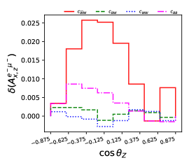
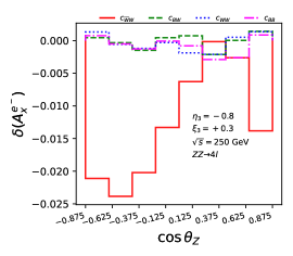
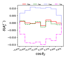
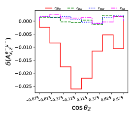
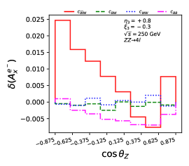
Figure 2: Relative change in asymmetries related to the CP-evenĀ (Pxsubscriptš‘ƒš‘„P_{x}) and CP-oddĀ (Pysubscriptš‘ƒš‘¦P_{y}) polarization and correlationĀ (Ax,zsubscriptš“š‘„š‘§A_{x,z}) where both the functions are CP-even. The distributions are shown for two set of beam polarization, Ī·3,Ī¾3=+0.8,āˆ’0.3formulae-sequencesubscriptšœ‚3subscriptšœ‰30.80.3\eta_{3},\xi_{3}=+0.8,-0.3Ā (in the top row) and the flipped polarizationĀ (in the bottom row) for four different anomalous couplings. The analysis is done at s=250š‘ 250\sqrt{s}=250Ā GeV, and at the rest frame of the mother particle.

The spin of a particle dictates the couplings with other fermions and bosons. These couplings are affected by the presence of higher-order operators; thus, understanding these couplings will serve as a window to probe deviations from the prediction of SM. The change in couplings may induce deviation in the values of various observables like crossĀ section, momenta, and angular distribution of final state particles. Some of the asymmetries constructed out of the angular distribution of final particles carry information on the spin of the mother particle in the form of polarization parameters. The polarization parameters are related to the dynamics of particle production; thus, these coefficients or spin-related observables can serve as a valuable tool for constraining the parameters of new physics. Generally, a particle with spin-sš‘ s provides 4ā€‹sā€‹(s+1)4š‘ š‘ 14s(s+1) polarization parameters, which are the independent parameters of the particle spin density matrix. For a spin-1 particle like Zš‘Z boson, the spin density matrix can be parameterized in Cartesian form as,

Pā€‹(Ī»,Ī»ā€²)=13ā€‹[I+32ā€‹Pā†’ā‹…Sā†’+32ā€‹Tiā€‹jā€‹{Si,Sj}],š‘ƒšœ†superscriptšœ†ā€²13delimited-[]š¼ā‹…32ā†’š‘ƒā†’š‘†32subscriptš‘‡š‘–š‘—subscriptš‘†š‘–subscriptš‘†š‘—P(\lambda,\lambda^{\prime})=\frac{1}{3}\left[I+\frac{3}{2}\vec{P}\cdot\vec{S}+\sqrt{\frac{3}{2}}T_{ij}\{S_{i},S_{j}\}\right], (16)

where Pā†’ā†’š‘ƒ\vec{P} and Tiā€‹jsubscriptš‘‡š‘–š‘—T_{ij} are the vector and tensor polarization parameters of Zš‘Z boson respectively and Sā†’ā†’š‘†\vec{S} is the spin-1 operator. To estimate them, one can calculate the parameters from the production density matrix, which is proportional to the product of the production amplitudes for different helicities of the Zš‘Z boson, Ļā€‹(Ī»,Ī»ā€²)āˆMā€‹(Ī»)ā€‹Mā‹†ā€‹(Ī»ā€²)proportional-tošœŒšœ†superscriptšœ†ā€²š‘€šœ†superscriptš‘€ā‹†superscriptšœ†ā€²\rho(\lambda,\lambda^{\prime})\propto M(\lambda)M^{\star}(\lambda^{\prime}), where Ī»āˆˆ{āˆ’,0,+}šœ†0\lambda\in\{-,0,+\}. Alternatively, one can constraint them at the decay level using the angular distribution of the decay products as in collider experiments. In this article, we focus on constructing polarization of Zš‘Z boson using the later methods. The angular distribution of fermions decayed from a spin-1 boson is written asĀ [60],

1Ļƒdā€‹Ļƒdā€‹Ī©=38ā€‹Ļ€[(23āˆ’(1āˆ’3Ī“)Tzā€‹z6)+Ī±PzcosĪø+32ā€‹(1āˆ’3ā€‹Ī“)ā€‹Tzā€‹zā€‹cos2ā”Īø+(Ī±ā€‹Px+2ā€‹23ā€‹(1āˆ’3ā€‹Ī“)ā€‹Txā€‹zā€‹cosā”Īø)Ɨsinā”Īøā€‹cosā”Īø+(Ī±ā€‹px+2ā€‹23ā€‹(1āˆ’3ā€‹Ī“)ā€‹Tyā€‹zā€‹cosā”Īø)ā€‹sinā”Īøā€‹sinā”Ļ•+(1āˆ’3Ī“)sin2Īø{(Txā€‹xāˆ’Tyā€‹y6)cosā”(2ā€‹Ļ•)+23Txā€‹ysinā”(2ā€‹Ļ•)}].1šœŽš‘‘šœŽš‘‘Ī©38šœ‹delimited-[]2313š›æsubscriptš‘‡š‘§š‘§6š›¼subscriptš‘ƒš‘§šœƒ3213š›æsubscriptš‘‡š‘§š‘§superscript2šœƒš›¼subscriptš‘ƒš‘„22313š›æsubscriptš‘‡š‘„š‘§šœƒšœƒšœƒš›¼subscriptš‘š‘„22313š›æsubscriptš‘‡š‘¦š‘§šœƒšœƒitalic-Ļ•13š›æsuperscript2šœƒsubscriptš‘‡š‘„š‘„subscriptš‘‡š‘¦š‘¦62italic-Ļ•23subscriptš‘‡š‘„š‘¦2italic-Ļ•\begin{split}&\frac{1}{\sigma}\frac{d\sigma}{d\Omega}=\frac{3}{8\pi}\left[\left(\frac{2}{3}-(1-3\delta)\frac{T_{zz}}{\sqrt{6}}\right)+\alpha P_{z}\cos\theta\right.\\ &+\left.\sqrt{\frac{3}{2}}(1-3\delta)T_{zz}\cos^{2}\theta+\left(\alpha P_{x}+2\sqrt{\frac{2}{3}}(1-3\delta)T_{xz}\cos\theta\right)\right.\\ &\times\left.\sin\theta\cos\theta+\left(\alpha p_{x}+2\sqrt{\frac{2}{3}}(1-3\delta)T_{yz}\cos\theta\right)\sin\theta\sin\phi\right.\\ &+\left.(1-3\delta)\sin^{2}\theta\left\{\left(\frac{T_{xx}-T_{yy}}{\sqrt{6}}\right)\cos(2\phi)\right.\right.\\ &+\left.\left.\sqrt{\frac{2}{3}}T_{xy}\sin(2\phi)\right\}\right].\end{split} (17)

Here, Īø,Ļ•šœƒitalic-Ļ•\theta,\phi are the polar and azimuthal angle of the final state fermion in the rest frame of the Zš‘Z boson with its would-be momentum along the zš‘§z-direction and xāˆ’zš‘„š‘§x-z plane being the lab frame production plane. The parameters Ī±š›¼\alpha and Ī“š›æ\delta depend on the chiral couplings and ratio of the mass of final state fermions to the mass of resonance, such that at the limit of massless fermions, Ī±ā†’Rf2āˆ’Lf2Rf2+Lf2ā†’š›¼subscriptsuperscriptš‘…2š‘“subscriptsuperscriptšæ2š‘“subscriptsuperscriptš‘…2š‘“subscriptsuperscriptšæ2š‘“\alpha\to\frac{R^{2}_{f}-L^{2}_{f}}{R^{2}_{f}+L^{2}_{f}} and Ī“ā†’0ā†’š›æ0\delta\to 0Ā [60]. At the decay level, one can calculate various asymmetries related to polarization and spin correlation parameters by taking the partial integration of Eq.Ā (17) w.r.t Īøšœƒ\theta and Ļ•italic-Ļ•\phi. For example, we can get Pxsubscriptš‘ƒš‘„P_{x} from the left-right asymmetry asĀ [60],

Axsubscriptš“š‘„\displaystyle A_{x} =1Ļƒā€‹[āˆ«Īø=0Ļ€āˆ«Ļ•=āˆ’Ļ€2Ļ€2dā€‹Ļƒdā€‹Ī©ā€‹š‘‘Ī©āˆ’āˆ«Īø=0Ļ€āˆ«Ļ•=Ļ€23ā€‹Ļ€2dā€‹Ļƒdā€‹Ī©ā€‹š‘‘Ī©]absent1šœŽdelimited-[]superscriptsubscriptšœƒ0šœ‹superscriptsubscriptitalic-Ļ•šœ‹2šœ‹2š‘‘šœŽš‘‘Ī©differential-dĪ©superscriptsubscriptšœƒ0šœ‹superscriptsubscriptitalic-Ļ•šœ‹23šœ‹2š‘‘šœŽš‘‘Ī©differential-dĪ©\displaystyle=\frac{1}{\sigma}\left[\int_{\theta=0}^{\pi}\int_{\phi=-\frac{\pi}{2}}^{\frac{\pi}{2}}\frac{d\sigma}{d\Omega}d\Omega-\int_{\theta=0}^{\pi}\int_{\phi=\frac{\pi}{2}}^{3\frac{\pi}{2}}\frac{d\sigma}{d\Omega}d\Omega\right] (18)
=3ā€‹Ī±ā€‹Px4=Ļƒā€‹(fx>0)āˆ’Ļƒā€‹(fx<0)Ļƒā€‹(fx>0)+Ļƒā€‹(fx<0),absent3š›¼subscriptš‘ƒš‘„4šœŽsubscriptš‘“š‘„0šœŽsubscriptš‘“š‘„0šœŽsubscriptš‘“š‘„0šœŽsubscriptš‘“š‘„0\displaystyle=\frac{3\alpha P_{x}}{4}=\frac{\sigma(f_{x}>0)-\sigma(f_{x}<0)}{\sigma(f_{x}>0)+\sigma(f_{x}<0)},

where fx=sinā”Īøā€‹cosā”Ļ•subscriptš‘“š‘„šœƒitalic-Ļ•f_{x}=\sin\theta\cos\phi. Likewise, the other angular functions used to construct the asymmetries are fy=sinā”Īøā€‹sinā”Ļ•subscriptš‘“š‘¦šœƒitalic-Ļ•f_{y}=\sin\theta\sin\phi, fz=cosā”Īøsubscriptš‘“š‘§šœƒf_{z}=\cos\theta, fxā€‹y=fxā€‹fysubscriptš‘“š‘„š‘¦subscriptš‘“š‘„subscriptš‘“š‘¦f_{xy}=f_{x}f_{y}, fxā€‹z=fxā€‹fzsubscriptš‘“š‘„š‘§subscriptš‘“š‘„subscriptš‘“š‘§f_{xz}=f_{x}f_{z}, fyā€‹z=fyā€‹fzsubscriptš‘“š‘¦š‘§subscriptš‘“š‘¦subscriptš‘“š‘§f_{yz}=f_{y}f_{z}, fx2āˆ’y2=fx2āˆ’fy2subscriptš‘“superscriptš‘„2superscriptš‘¦2superscriptsubscriptš‘“š‘„2superscriptsubscriptš‘“š‘¦2f_{x^{2}-y^{2}}=f_{x}^{2}-f_{y}^{2}, and fzā€‹z=1āˆ’fz2ā€‹[3āˆ’4ā€‹(1āˆ’fz2)]subscriptš‘“š‘§š‘§1superscriptsubscriptš‘“š‘§2delimited-[]341superscriptsubscriptš‘“š‘§2f_{zz}=\sqrt{1-f_{z}^{2}}\left[3-4(1-f_{z}^{2})\right]. The asymmetries related to other polarization parameters are obtained similarly using the above function.

When two particles are co-produced, their spin is correlated owing to the conservation of angular momentum. In general, for two particles Aš“A and BšµB with spin sAsubscriptš‘ š“s_{A} and sBsubscriptš‘ šµs_{B} respectively, there are 16ā€‹sAā€‹sBā€‹(sA+1)ā€‹(sB+1)16subscriptš‘ š“subscriptš‘ šµsubscriptš‘ š“1subscriptš‘ šµ116s_{A}s_{B}(s_{A}+1)(s_{B}+1) spin correlation parameters. The total rate for the production of two spin-1 particles followed by their decay, .i.e, Aā†’aā€‹aā€²ā†’š“š‘Žsuperscriptš‘Žā€²A\to aa^{\prime} and Bā†’bā€‹bā€²ā†’šµš‘superscriptš‘ā€²B\to bb^{\prime} can be written asĀ [61],

1Ļƒā€‹dā€‹Ļƒdā€‹Ī©aā€‹dā€‹Ī©b=1šœŽš‘‘šœŽš‘‘subscriptĪ©š‘Žš‘‘subscriptĪ©š‘absent\displaystyle\frac{1}{\sigma}\frac{d\sigma}{d\Omega_{a}d\Omega_{b}}= 916ā€‹Ļ€2ā€‹āˆ‘Ī»A,Ī»Aā€²,Ī»B,Ī»Bā€²PAā€‹Bā€‹(Ī»A,Ī»Aā€²,Ī»B,Ī»Bā€²)916superscriptšœ‹2subscriptsubscriptšœ†š“superscriptsubscriptšœ†š“ā€²subscriptšœ†šµsuperscriptsubscriptšœ†šµā€²subscriptš‘ƒš“šµsubscriptšœ†š“superscriptsubscriptšœ†š“ā€²subscriptšœ†šµsuperscriptsubscriptšœ†šµā€²\displaystyle\frac{9}{16\pi^{2}}\sum_{\lambda_{A},\lambda_{A}^{\prime},\lambda_{B},\lambda_{B}^{\prime}}P_{AB}(\lambda_{A},\lambda_{A}^{\prime},\lambda_{B},\lambda_{B}^{\prime}) (19)
Ī“Aā€‹(Ī»A,Ī»Aā€²)ā€‹Ī“Bā€‹(Ī»B,Ī»Bā€²).subscriptĪ“š“subscriptšœ†š“superscriptsubscriptšœ†š“ā€²subscriptĪ“šµsubscriptšœ†šµsuperscriptsubscriptšœ†šµā€²\displaystyle\Gamma_{A}(\lambda_{A},\lambda_{A}^{\prime})\Gamma_{B}(\lambda_{B},\lambda_{B}^{\prime}).

PAā€‹Bsubscriptš‘ƒš“šµP_{AB} represents the joint polarization density matrix. Moreover, similarly, by using the respective form for the density matrix, one obtains the joint angular distribution of the decay products of Aš“A and BšµB. In the case of two spin-1 particles, there will be 64 spin correlation parameters, which can be obtained using different angular functions asĀ [61],

š’œiā€‹jAā€‹B=Ļƒā€‹(fiaā€‹fjb>0)āˆ’Ļƒā€‹(fiaā€‹fjb<0)Ļƒā€‹(fiaā€‹fjb>0)+Ļƒā€‹(fiaā€‹fjb<0).superscriptsubscriptš’œš‘–š‘—š“šµšœŽsubscriptsuperscriptš‘“š‘Žš‘–subscriptsuperscriptš‘“š‘š‘—0šœŽsubscriptsuperscriptš‘“š‘Žš‘–subscriptsuperscriptš‘“š‘š‘—0šœŽsubscriptsuperscriptš‘“š‘Žš‘–subscriptsuperscriptš‘“š‘š‘—0šœŽsubscriptsuperscriptš‘“š‘Žš‘–subscriptsuperscriptš‘“š‘š‘—0\mathcal{A}_{ij}^{AB}=\frac{\sigma(f^{a}_{i}f^{b}_{j}>0)-\sigma(f^{a}_{i}f^{b}_{j}<0)}{\sigma(f^{a}_{i}f^{b}_{j}>0)+\sigma(f^{a}_{i}f^{b}_{j}<0)}. (20)

It is worth noting that the asymmetries defined above can be divided into CP-even and CP-odd observables. Three of the polarization asymmetries are CP-odd, and five are CP-even. In the case of spin correlations, there are 34 CP-even and 30 CP-odd asymmetries. In Fig.Ā 2, we show the relative change of asymmetries value in presence of anomalous couplings by keeping one anomalous couplings to non-zero at a time while other are set to zero. The benchmark anomalous point is kept to 100Ā TeV-2 for each new physics parameter. In particular, we show the variation for asymmetriesĀ (polarization) related to the angular distribution of fxeāˆ’ā€‹(Axeāˆ’)superscriptsubscriptš‘“š‘„superscriptš‘’superscriptsubscriptš“š‘„superscriptš‘’f_{x}^{e^{-}}~{}(A_{x}^{e^{-}}), fyeāˆ’ā€‹(Ayeāˆ’)superscriptsubscriptš‘“š‘¦superscriptš‘’superscriptsubscriptš“š‘¦superscriptš‘’f_{y}^{e^{-}}~{}(A_{y}^{e^{-}}) and correlation of functionĀ fxeāˆ’ā€‹fzĪ¼āˆ’ā€‹(Ax,zeāˆ’ā€‹Ī¼āˆ’)superscriptsubscriptš‘“š‘„superscriptš‘’superscriptsubscriptš‘“š‘§superscriptšœ‡superscriptsubscriptš“š‘„š‘§superscriptš‘’superscriptšœ‡f_{x}^{e^{-}}f_{z}^{\mu^{-}}~{}(A_{x,z}^{e^{-}\mu^{-}}). We perform this analysis at center-of-mass energy of 250250250Ā GeV, with two set of initial beam polarization (Ī·3,Ī¾3)=(+0.8,āˆ’0.3)subscriptšœ‚3subscriptšœ‰30.80.3(\eta_{3},\xi_{3})=(+0.8,-0.3)Ā (shown in the top row) and the flipped polarizationĀ (in the bottom row). In Fig.Ā 2, we see that the variation in the asymmetries for CP-odd anomalous couplings, ciāˆˆ{cWā€‹W,cBā€‹B,cBā€‹W}subscriptš‘š‘–subscriptš‘š‘Šš‘Šsubscriptš‘šµšµsubscriptš‘šµš‘Šc_{i}\in\{c_{WW},c_{BB},c_{BW}\} are minimal while the variation are significant for CP-even asymmetries like Axsubscriptš“š‘„A_{x}, and Ax,zeāˆ’ā€‹Ī¼āˆ’superscriptsubscriptš“š‘„š‘§superscriptš‘’superscriptšœ‡A_{x,z}^{e^{-}\mu^{-}}, while it provides significant change in CP-odd asymmetriesĀ (Ayeāˆ’superscriptsubscriptš“š‘¦superscriptš‘’A_{y}^{e^{-}}). Further, in case of CP-even asymmetries the sign of the relative change in asymmetries gets flipped in the case when the beam polarization is flipped. Thus, various asymmetries might act as an analyzer for the CP state of the new physics. The change in the asymmetries due to anomalous couplings are non-symmetric to the cosā”ĪøZsubscriptšœƒš‘\cos\theta_{Z} related to the Zš‘Z boson. E.g., in the case of asymmetries related to Ax,zsubscriptš“š‘„š‘§A_{x,z}, the maximal change from the SM value is seen for āˆ’0.5<cosā”ĪøZ<0.50.5subscriptšœƒš‘0.5-0.5<\cos\theta_{Z}<0.5 region, and in the case of Axsubscriptš“š‘„A_{x}, the change follows a asymmetric distribution in the range āˆ’1.0<cosā”ĪøZ<+1.01.0subscriptšœƒš‘1.0-1.0<\cos\theta_{Z}<+1.0. This asymmetric change w.r.t cosā”ĪøZsubscriptšœƒš‘\cos\theta_{Z} allows one to bin the asymmetries in a specific range of cosā”ĪøZsubscriptšœƒš‘\cos\theta_{Z}.

In the next section, we discuss the methodology and the limits obtained on various anomalous couplings. We will also emphasize the role of statistical and systematic errors in setting the bounds on anomalous couplings.

III Probe of anomalous couplings

This section presents a comprehensive methodology for obtaining bounds on anomalous couplings, denoted by cisubscriptš‘š‘–c_{i}, in the context of Zā€‹Zš‘š‘ZZ and Zā€‹Ī³š‘š›¾Z\gamma processes. Our approach involves dividing all the observables into eight bins of cosā”ĪøZsubscriptšœƒš‘\cos\theta_{Z}, where ĪøZsubscriptšœƒš‘\theta_{Z} represents the production angle of the Zš‘Z boson in the laboratory frame. This allows us to increase the number of observables and better constrain the anomalous couplings. This strategy has the advantage of fine-tuning the distinction between the signal resulting from new physics and the SM forecast. The ability to detect and eliminate differences between the SM predictions and experimental data is made possible by the growth in observables, which in turn allows us to impose stricter limits on anomalous couplings. The event simulations are carried out using the Monte Carlo method implemented in MadGraph5__\_aMC@@@NLOĀ [23], which allows us to simulate the production and decay of Zā€‹Zš‘š‘ZZ and Zā€‹Ī³š‘š›¾Z\gamma bosons in the presence of anomalous couplings. The resulting simulated events are then analyzed to extract the relevant observables, which are divided into the eight bins mentioned above of cosā”ĪøZsubscriptšœƒš‘\cos\theta_{Z}.

Next, we fit the values of the observables in each bin to derive a semi-analytical expression for all observables as a function of the anomalous couplings. This enables us to establish the relationship between the observables and the anomalous couplings and to derive the most likely values of the couplings that best fit the data. In presence of anomalous couplings, cisubscriptš‘š‘–c_{i}, the crossĀ section is fitted using the following parameterization,

ĻƒšœŽ\displaystyle\sigma =Ļƒ0+Ļƒiā€‹ci+āˆ‘jā‰ kĻƒjā€‹kā€‹cjā€‹ck+āˆ‘l=14Ļƒlā€‹lā€‹cl2,absentsubscriptšœŽ0subscriptšœŽš‘–subscriptš‘š‘–subscriptš‘—š‘˜subscriptšœŽš‘—š‘˜subscriptš‘š‘—subscriptš‘š‘˜superscriptsubscriptš‘™14subscriptšœŽš‘™š‘™superscriptsubscriptš‘š‘™2\displaystyle=\sigma_{0}+\sigma_{i}c_{i}+\sum_{j\neq k}\sigma_{jk}c_{j}c_{k}+\sum_{l=1}^{4}\sigma_{ll}c_{l}^{2}, (21)
i=cB~ā€‹W,j,kāˆˆ{cBā€‹W,cWā€‹W,cBā€‹B},l=iāˆŖj.formulae-sequenceš‘–subscriptš‘~šµš‘Šš‘—formulae-sequenceš‘˜subscriptš‘šµš‘Šsubscriptš‘š‘Šš‘Šsubscriptš‘šµšµš‘™š‘–š‘—\displaystyle i=c_{\widetilde{B}W},j,k\in\{c_{BW},c_{WW},c_{BB}\},l=i\cup j.

The numerator and denominator are fitted independently for asymmetries and then used as

š’œiā€‹({ci})=Ī”ā€‹Ļƒš’œiā€‹({ci})Ļƒā€‹({ci}).subscriptš’œš‘–subscriptš‘š‘–Ī”subscriptšœŽsubscriptš’œš‘–subscriptš‘š‘–šœŽsubscriptš‘š‘–\mathcal{A}_{i}(\{c_{i}\})=\frac{\Delta\sigma_{\mathcal{A}_{i}}(\{c_{i}\})}{\sigma(\{c_{i}\})}. (22)

The denominator is the crossĀ section which is fitted as in Eq.Ā (21), and the numerator of CP-odd asymmetries is fitted as,

Ī”ā€‹Ļƒš’œiā€‹({ci})Ī”subscriptšœŽsubscriptš’œš‘–subscriptš‘š‘–\displaystyle\Delta\sigma_{\mathcal{A}_{i}}(\{c_{i}\}) =āˆ‘iĻƒiā€‹ci+āˆ‘iĻƒ1ā€‹iā€‹cB~ā€‹Wā€‹ci,absentsubscriptš‘–subscriptšœŽš‘–subscriptš‘š‘–subscriptš‘–subscriptšœŽ1š‘–subscriptš‘~šµš‘Šsubscriptš‘š‘–\displaystyle=\sum_{i}\sigma_{i}c_{i}+\sum_{i}\sigma_{1i}c_{\widetilde{B}W}c_{i}, (23)
iāˆˆ{cBā€‹W,cWā€‹W,cBā€‹B}.š‘–subscriptš‘šµš‘Šsubscriptš‘š‘Šš‘Šsubscriptš‘šµšµ\displaystyle i\in\{c_{BW},c_{WW},c_{BB}\}.
Refer to caption
Refer to caption
Refer to caption
Refer to caption
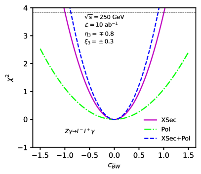
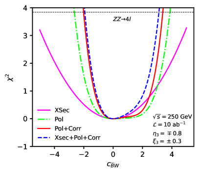
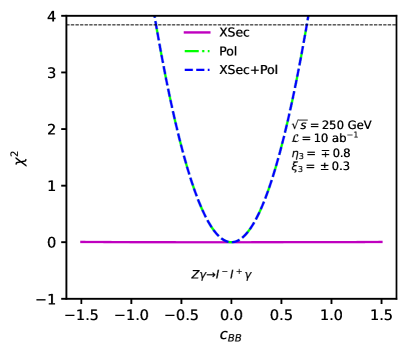
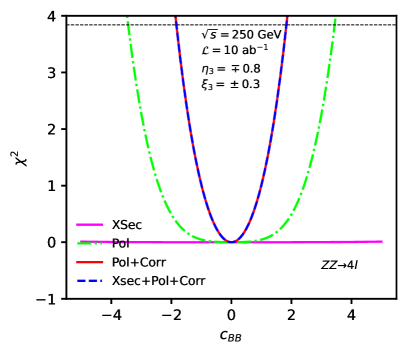
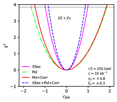
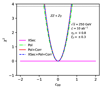
Figure 3: One dimensional Ļ‡2superscriptšœ’2\chi^{2} for cross-section, polarizations, combinations of polarization and spin-spin correlations and combinations of all observables as a function of one anomalous couplings at a time for a Zā€‹Zā†’4ā€‹lā†’š‘š‘4š‘™ZZ\to 4l and Zā€‹Ī³ā†’lāˆ’ā€‹l+ā€‹Ī³ā†’š‘š›¾superscriptš‘™superscriptš‘™š›¾Z\gamma\to l^{-}l^{+}\gamma process. The plots are obtained at s=250š‘ 250\sqrt{s}=250 GeV, ā„’=10ā„’10\mathcal{L}=10 ab-1 and zero systematic errors. The horizontal line at Ļ‡2=3.84superscriptšœ’23.84\chi^{2}=3.84 corresponds to the limits of anomalous couplings at 95%percent\% confidence levelĀ (CL).

When dealing with events with two sets of beam polarization, merging the different sets at the Ļ‡2superscriptšœ’2\chi^{2} level yields more stringent constraintsĀ [62]. The combined Ļ‡2superscriptšœ’2\chi^{2} at different set of beam polarizationĀ (Ā±Ī·3,āˆ“Ī¾3plus-or-minussubscriptšœ‚3minus-or-plussubscriptšœ‰3\pm\eta_{3},\mp\xi_{3}), and using different observable š’Ŗš’Ŗ\mathcal{O} for a given value of anomalous couplings cisubscriptš‘š‘–c_{i} is defined as,

Ļ‡2ā€‹(š’Ŗ,ci,Ā±Ī·3,āˆ“Ī¾3)=superscriptšœ’2š’Ŗsubscriptš‘š‘–plus-or-minussubscriptšœ‚3minus-or-plussubscriptšœ‰3absent\displaystyle\chi^{2}(\mathcal{O},c_{i},\pm\eta_{3},\mp\xi_{3})= (24)
āˆ‘l,k[(š’Ŗklā€‹(ci,+Ī·3,āˆ’Ī¾3)āˆ’š’Ŗklā€‹(0,+Ī·3,āˆ’Ī¾3)Ī“ā€‹š’Ŗklā€‹(0,+Ī·3,āˆ’Ī¾3))2\displaystyle\sum_{l,k}\left[\left(\frac{\mathscr{O}_{k}^{l}(c_{i},+\eta_{3},-\xi_{3})-\mathscr{O}_{k}^{l}(0,+\eta_{3},-\xi_{3})}{\delta\mathscr{O}^{l}_{k}(0,+\eta_{3},-\xi_{3})}\right)^{2}\right.
+(š’Ŗklā€‹(ci,āˆ’Ī·3,+Ī¾3)āˆ’š’Ŗklā€‹(0,āˆ’Ī·3,+Ī¾3)Ī“ā€‹š’Ŗklā€‹(0,āˆ’Ī·3,+Ī¾3))2],\displaystyle\left.+\left(\frac{\mathscr{O}_{k}^{l}(c_{i},-\eta_{3},+\xi_{3})-\mathscr{O}_{k}^{l}(0,-\eta_{3},+\xi_{3})}{\delta\mathscr{O}^{l}_{k}(0,-\eta_{3},+\xi_{3})}\right)^{2}\right],

where k,lš‘˜š‘™k,l runs over all bins and observables separately, and Ī“ā€‹š’Ŗ=(Ī“ā€‹š’Ŗstat)2+(Ī“ā€‹š’Ŗsyst)2š›æš’Ŗsuperscriptš›æsubscriptš’Ŗstat2superscriptš›æsubscriptš’Ŗsyst2\delta\mathcal{O}=\sqrt{(\delta\mathcal{O}_{\text{stat}})^{2}+(\delta\mathcal{O}_{\text{syst}})^{2}} is the estimated error in š’Ŗš’Ŗ\mathcal{O}. For crossĀ section ĻƒšœŽ\sigma, the estimated error is given by,

Ī“ā€‹Ļƒ=Ļƒā„’+(ĻµĻƒā€‹Ļƒ)2,š›æšœŽšœŽā„’superscriptsubscriptitalic-ĻµšœŽšœŽ2\delta\sigma=\sqrt{\frac{\sigma}{\mathcal{L}}+(\epsilon_{\sigma}\sigma)^{2}}, (25)

and if the observable is asymmetry, the error is given by,

Ī“ā€‹š’œ=1āˆ’š’œ2ā„’ā€‹Ļƒ+Ļµš’œ2.š›æš’œ1superscriptš’œ2ā„’šœŽsuperscriptsubscriptitalic-Ļµš’œ2\delta\mathcal{A}=\sqrt{\frac{1-\mathcal{A}^{2}}{\mathcal{L}\sigma}+\epsilon_{\mathcal{A}}^{2}}. (26)

Here, Ļµš’œ,ĻµĻƒsubscriptitalic-Ļµš’œsubscriptitalic-ĻµšœŽ\epsilon_{\mathcal{A}},\epsilon_{\sigma} are the systematic error in asymmetry and crossĀ section, respectively, and ā„’ā„’\mathcal{L} is the integrated luminosity. The chi-squared analysis provides complete information on the sensitivity of observables along with the constraint on anomalous couplings.

Refer to caption
Refer to caption
Figure 4: One dimensional combined Ļ‡2superscriptšœ’2\chi^{2} for different sets of observables as a function of anomalous couplingsĀ (ciāˆˆ{cB~ā€‹W,cBā€‹W}subscriptš‘š‘–subscriptš‘~šµš‘Šsubscriptš‘šµš‘Šc_{i}\in\{c_{\widetilde{B}W},c_{BW}\}). The horizontal line at Ļ‡2=3.84superscriptšœ’23.84\chi^{2}=3.84 denotes limits at 95%percent9595\% CL. The analysis is done with zero systematic error.

The analysis are performed at s=250š‘ 250\sqrt{s}=250Ā GeV with different values of integrated luminosity,

ā„’āˆˆ{0.1ā€‹abāˆ’1,0.3ā€‹abāˆ’1,1ā€‹abāˆ’1,3ā€‹ab1āˆ’,10ā€‹abāˆ’1}.\mathcal{L}\in\{0.1~{}\text{ab}^{-1},0.3~{}\text{ab}^{-1},1~{}\text{ab}^{-1},3~{}\text{ab}^{{}^{-}1},10~{}\text{ab}^{-1}\}. (27)

The SM crossĀ sections for Zā€‹Zā†’eāˆ’ā€‹e+ā€‹Ī¼āˆ’ā€‹Ī¼+ā†’š‘š‘superscriptš‘’superscriptš‘’superscriptšœ‡superscriptšœ‡ZZ\to e^{-}e^{+}\mu^{-}\mu^{+} and Zā€‹Ī³ā†’lāˆ’ā€‹l+ā€‹Ī³ā†’š‘š›¾superscriptš‘™superscriptš‘™š›¾Z\gamma\to l^{-}l^{+}\gamma process at s=250š‘ 250\sqrt{s}=250 GeV with two set of initial beam polarization of (Ā±0.8,āˆ“0.3plus-or-minus0.8minus-or-plus0.3\pm 0.8,\mp 0.3) are,

ĻƒZā€‹Zā€‹(+0.8,āˆ’0.3)=2.15ā€‹fb,subscriptšœŽš‘š‘0.80.32.15fb\displaystyle\sigma_{ZZ}(+0.8,-0.3)=2.15~{}\text{fb}, (28)
ĻƒZā€‹Zā€‹(āˆ’0.8,+0.3)=3.41ā€‹fb,subscriptšœŽš‘š‘0.80.33.41fb\displaystyle\sigma_{ZZ}(-0.8,+0.3)=3.41~{}\text{fb},
ĻƒZā€‹Ī³ā€‹(+0.8,āˆ’0.3)=607.62ā€‹fb,subscriptšœŽš‘š›¾0.80.3607.62fb\displaystyle\sigma_{Z\gamma}(+0.8,-0.3)=607.62~{}\text{fb},
ĻƒZā€‹Ī³ā€‹(āˆ’0.8,+0.3)=765.83ā€‹fb.subscriptšœŽš‘š›¾0.80.3765.83fb\displaystyle\sigma_{Z\gamma}(-0.8,+0.3)=765.83~{}\text{fb}.

Given the crossĀ section as in Eq.Ā (28) and luminosity in Eq.Ā (27), the relative statistical error as obtained from Eq.Ā (25) are,

Ī“ā€‹ĻƒĻƒā€‹(+0.8,āˆ’0.3)|Zā€‹Zevaluated-atš›æšœŽšœŽ0.80.3š‘š‘\displaystyle\frac{\delta\sigma}{\sigma}(+0.8,-0.3)|_{ZZ} ={6.81%,3.93%,2.15%,1.24%,0.68%},absentpercent6.81percent3.93percent2.15percent1.24percent0.68\displaystyle=\{6.81\%,3.93\%,2.15\%,1.24\%,0.68\%\}, (29)
Ī“ā€‹ĻƒĻƒā€‹(āˆ’0.8,+0.3)|Zā€‹Zevaluated-atš›æšœŽšœŽ0.80.3š‘š‘\displaystyle\frac{\delta\sigma}{\sigma}(-0.8,+0.3)|_{ZZ} ={5.40%,3.12%,1.71%,0.98%,0.54%},absentpercent5.40percent3.12percent1.71percent0.98percent0.54\displaystyle=\{5.40\%,3.12\%,1.71\%,0.98\%,0.54\%\},
Ī“ā€‹ĻƒĻƒā€‹(+0.8,āˆ’0.3)|Zā€‹Ī³evaluated-atš›æšœŽšœŽ0.80.3š‘š›¾\displaystyle\frac{\delta\sigma}{\sigma}(+0.8,-0.3)|_{Z\gamma} ={0.40%,0.23%,0.12%,0.07%,0.04%},absentpercent0.40percent0.23percent0.12percent0.07percent0.04\displaystyle=\{0.40\%,0.23\%,0.12\%,0.07\%,0.04\%\},
Ī“ā€‹ĻƒĻƒā€‹(āˆ’0.8,+0.3)|Zā€‹Ī³evaluated-atš›æšœŽšœŽ0.80.3š‘š›¾\displaystyle\frac{\delta\sigma}{\sigma}(-0.8,+0.3)|_{Z\gamma} ={0.36%,0.20%,0.11%,0.06%,0.03%}.absentpercent0.36percent0.20percent0.11percent0.06percent0.03\displaystyle=\{0.36\%,0.20\%,0.11\%,0.06\%,0.03\%\}.
Refer to caption
Refer to caption
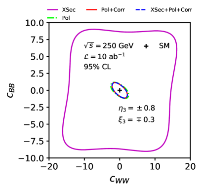
Figure 5: 2-D 95%percent\% CL contours of Ļ‡2superscriptšœ’2\chi^{2} for cross-section, polarizations, spin correlations and their combinations as a function of two anomalous couplings at a time for combined Zā€‹Zš‘š‘ZZ and Zā€‹Ī³š‘š›¾Z\gammaprocess. The analysis is done at center of mass energy s=250š‘ 250\sqrt{s}=250 GeV, integrated luminosity ā„’=10ā„’10\mathcal{L}=10 ab-1 and systematic error are chosen to be zero. The cross in the center represents SM points.

The above statistical error is given for a unbinned events, while for the binnedĀ (eight bin) case the statistical error increases depending on the rate. On top of the statistical error given in the above equation, we add systematic error given as,

(ĻµĻƒ,Ļµš’œ)={(0,0),(0.5%,0.25%),(2%,1%)}.subscriptitalic-ĻµšœŽsubscriptitalic-Ļµš’œ00percent0.5percent0.25percent2percent1(\epsilon_{\sigma},\epsilon_{\mathcal{A}})=\{(0,0),(0.5\%,0.25\%),(2\%,1\%)\}. (30)

In the case of Zā€‹Zā†’4ā€‹lā†’š‘š‘4š‘™ZZ\to 4l events, the estimated error is primarily dominated by the statistical component within the regime of systematic error given by Eq.Ā (30) due to the low branching ratio of the full lepton channel. It implies that the sensitivity of various observables would increase with luminosity, while for the case of Zā€‹Ī³š‘š›¾Z\gamma process the net error saturates for given non-zero value of systematic error.

The figures presented in Fig.Ā 3 depict the Ļ‡2superscriptšœ’2\chi^{2} analysis performed for various sets of observables as a function of one anomalous coupling at a time for two different final topologies: 4ā€‹l4š‘™4l and lāˆ’ā€‹l+ā€‹Ī³superscriptš‘™superscriptš‘™š›¾l^{-}l^{+}\gamma. The analysis is carried with an integrated luminosity of ā„’=10ā„’10\mathcal{L}=10 ab-1, and with systematic errors chosen to be zero. The beams are polarized with a degree of polarization Ī·3=Ā±0.8subscriptšœ‚3plus-or-minus0.8\eta_{3}=\pm 0.8 and Ī¾3=āˆ“0.3subscriptšœ‰3minus-or-plus0.3\xi_{3}=\mp 0.3.
Each panel of Fig.Ā 3 illustrates that the dominant contribution to constraining anomalous couplings arises from the spin-related observables, which are combinations of the polarization and spin-spin correlation parameters. For CP-odd couplings in the bottom row of the Fig.Ā 3, the limits set by these spin-related observables remain unaffected by the presence of a crossĀ section. This is because, in the case of CP-even observables like crossĀ section, the contribution from CP-odd couplings only arises at the 1/Ī›81superscriptĪ›81/\Lambda^{8} term, whose contribution is sub-dominant compared to the linear contributionĀ (1/Ī›41superscriptĪ›41/\Lambda^{4}) from CP-even. In the presence of one anomalous coupling (cisubscriptš‘š‘–c_{i}), the CP-even observables can be parameterized by Eq.Ā (31),

Ļƒā€‹(ci)=Ļƒ0+Ļƒiā€‹ci+Ļƒiā€‹iā€‹ci2,šœŽsubscriptš‘š‘–subscriptšœŽ0subscriptšœŽš‘–subscriptš‘š‘–subscriptšœŽš‘–š‘–superscriptsubscriptš‘š‘–2\sigma(c_{i})=\sigma_{0}+\sigma_{i}c_{i}+\sigma_{ii}c_{i}^{2}, (31)

where Ļƒ0subscriptšœŽ0\sigma_{0} corresponds to the SM value. Therefore, the linear term in the crossĀ section is absent for CP-odd cisubscriptš‘š‘–c_{i}, leading to a negligible contribution. It is also evident from Fig.Ā 3 that the Zā€‹Ī³š‘š›¾Z\gamma process imposes a tighter constraint than the Zā€‹Zš‘š‘ZZ process in the case of CP-odd coupling, CBā€‹Bsubscriptš¶šµšµC_{BB} through combination of different polarization asymmetries. However, for the CP-even case, the crossĀ section provides tighter constraint than the polarization asymmetries in case of Zā€‹Ī³š‘š›¾Z\gamma process, while the limits for the same anomalous coupling from Zā€‹Zš‘š‘ZZ process is bit relaxed.

Refer to caption
Refer to caption
Refer to caption
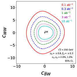
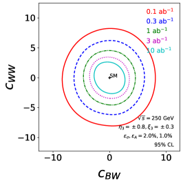
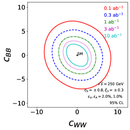
Figure 6: Two dimensional marginalized projections of the anomalous couplings cisubscriptš‘š‘–c_{i}Ā (TeV-4) at 95%percent\% CL obtained using MCMC global fits for a conservative systematic error (2.0%,1.0%)percent2.0percent1.0(2.0\%,1.0\%) and different values of integrated luminosities.
Refer to caption
Refer to caption
Refer to caption
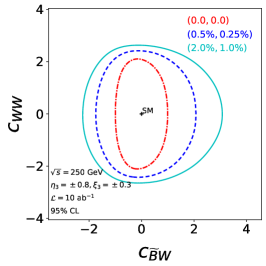
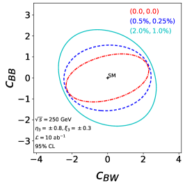
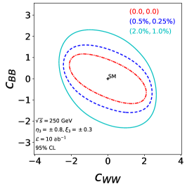
Figure 7: Two dimensional marginalized projections of the maximally correlated parameters cisubscriptš‘š‘–c_{i}Ā (TeV-4) at 95%percent\% CL obtained using MCMC global fits for a set of systematic error and integrated luminosity ā„’=10ā„’10\mathcal{L}=10 ab-1.

Next, we combine the two processes at the level of Ļ‡2superscriptšœ’2\chi^{2} as,

Ļ‡Tot2ā€‹({ci},Ā±Ī·3,āˆ“Ī¾3)subscriptsuperscriptšœ’2Totsubscriptš‘š‘–plus-or-minussubscriptšœ‚3minus-or-plussubscriptšœ‰3\displaystyle\chi^{2}_{\text{Tot}}(\{c_{i}\},\pm\eta_{3},\mp\xi_{3}) =Ļ‡Zā€‹Z2ā€‹({ci},Ā±Ī·3,āˆ“Ī¾3)absentsubscriptsuperscriptšœ’2š‘š‘subscriptš‘š‘–plus-or-minussubscriptšœ‚3minus-or-plussubscriptšœ‰3\displaystyle=\chi^{2}_{ZZ}(\{c_{i}\},\pm\eta_{3},\mp\xi_{3}) (32)
+Ļ‡Zā€‹Ī³2ā€‹({ci},Ā±Ī·3,āˆ“Ī¾3),subscriptsuperscriptšœ’2š‘š›¾subscriptš‘š‘–plus-or-minussubscriptšœ‚3minus-or-plussubscriptšœ‰3\displaystyle+\chi^{2}_{Z\gamma}(\{c_{i}\},\pm\eta_{3},\mp\xi_{3}),

where each Ļ‡2superscriptšœ’2\chi^{2} is obtained following Eq.Ā (24) and on obtaining the above defined Ļ‡2superscriptšœ’2\chi^{2}, we have consider the all other leptonic decay channel for Zā€‹Zš‘š‘ZZ process. The resultant one and two-dimensional Ļ‡2superscriptšœ’2\chi^{2} distribution for a set of observables as a function of one and two anomalous couplings at a time are shown in Fig.Ā 4 and Fig.Ā 5, respectively. The hierarchy of observables on setting the bounds on anomalous couplings is the same as described above for individual topology. For CP-odd case, the crossĀ section provides the least contribution to the Ļ‡2superscriptšœ’2\chi^{2}, and combinations of polarization and spin correlation asymmetries predominantly set the bounds. For the CP-even case, the crossĀ section contributes the most to Ļ‡2superscriptšœ’2\chi^{2} alone. The one parameter limits at 95%percent\% confidence levelĀ (CL) obtained from the combined analysis are listed in TableĀ 2, where it is evident that the Zā€‹Ī³š‘š›¾Z\gamma channel dominates the limits on most of the anomalous couplings, except for cBā€‹Wsubscriptš‘šµš‘Šc_{BW}.

Table 2: One parameter limits on anomalous couplingsĀ (cisubscriptš‘š‘–c_{i}) at 95%percent\% CL obtained for Zā€‹Zā†’4ā€‹lā†’š‘š‘4š‘™ZZ\to 4l, Zā€‹Ī³ā†’2ā€‹lā€‹Ī³ā†’š‘š›¾2š‘™š›¾Z\gamma\to 2l\gamma and their combinations. The limits are obtained at center of mass energy s=250š‘ 250\sqrt{s}=250 GeV, integrated luminosity ā„’=ā„’absent\mathcal{L}= 10 ab-1 and zero systematic.
ParametersĀ (cisubscriptš‘š‘–c_{i}) LimitsĀ (TeV-4)
Zā€‹Ī³ā†’2ā€‹lā€‹Ī³ā†’š‘š›¾2š‘™š›¾Z\gamma\to 2l\gamma Zā€‹Zā†’4ā€‹lā†’š‘š‘4š‘™ZZ\to 4l Zā€‹Z+Zā€‹Ī³š‘š‘š‘š›¾ZZ+Z\gamma
cB~ā€‹W/Ī›4subscriptš‘~šµš‘ŠsuperscriptĪ›4c_{\widetilde{B}W}/\Lambda^{4} [āˆ’0.88,+0.88]0.880.88[-0.88,+0.88] [āˆ’1.93,+3.11]1.933.11[-1.93,+3.11] [āˆ’0.83,+0.86]0.830.86[-0.83,+0.86]
cBā€‹W/Ī›4subscriptš‘šµš‘ŠsuperscriptĪ›4c_{BW}/\Lambda^{4} [āˆ’2.89,+2.89]2.892.89[-2.89,+2.89] [āˆ’2.40,+2.40]2.402.40[-2.40,+2.40] [āˆ’1.97,+1.97]1.971.97[-1.97,+1.97]
cWā€‹Wā€‹Ī›4subscriptš‘š‘Šš‘ŠsuperscriptĪ›4c_{WW}\Lambda^{4} [āˆ’1.75,+1.75]1.751.75[-1.75,+1.75] [āˆ’2.17,+2.17]2.172.17[-2.17,+2.17] [āˆ’1,42,+1.42]1421.42[-1,42,+1.42]
cBā€‹B/Ī›4subscriptš‘šµšµsuperscriptĪ›4c_{BB}/\Lambda^{4} [āˆ’0.75,+0.75]0.750.75[-0.75,+0.75] [āˆ’1.83,+1.83]1.831.83[-1.83,+1.83] [āˆ’0.70,+0.70]0.700.70[-0.70,+0.70]

The one parameter limits in the current workĀ (ILC @@@ 10Ā ab-1) are diluted for Zā€‹Ī³š‘š›¾Z\gamma process, while the limits are tighter for Zā€‹Zš‘š‘ZZ process, in contrast to the experimental limitĀ (LHC @@@ 36.1Ā fb-1) listed in TableĀ 1. Our current study examines the ILC potential to probe dim-8 bosonic operators without directly comparing it to existing colliders. Notably, the LHC boasts a higher collision energyĀ (ā‰ˆ\approx 2 TeV) compared to the ILCĀ (250 GeV). This makes the anomalous vertex more sensitive to the higher energy reach of LHC since the vertex created by dim-8 operators comprises the terms reliant on the momentum transfer normalized by the electroweak scale. Besides the energy domination at LHC, the cross-section of Zā€‹Ī³ā†’Ī½ā€‹Ī½ĀÆā€‹Ī³ā†’š‘š›¾šœˆĀÆšœˆš›¾Z\gamma\to\nu\bar{\nu}\gamma is ā‰ˆ25absent25\approx 25 times larger at ILC than it is for Zā€‹Ī³ā†’lāˆ’ā€‹l+ā€‹Ī³ā†’š‘š›¾superscriptš‘™superscriptš‘™š›¾Z\gamma\to l^{-}l^{+}\gamma, , while for Zā€‹Zā†’4ā€‹lā†’š‘š‘4š‘™ZZ\to 4l process the crossĀ section is ā‰ˆ9absent9\approx 9 times higher in LHC than at ILC. Nevertheless, the significant number of observables used in our analysis try to compensate for the low energy and crossĀ section, which is visible in Fig.Ā 4 where the limits on anomalous couplings become tighter on using polarizations and spin correlations. A recent studyĀ [25] achieved a comparable limit on anomalous couplings at greater energy s=500š‘ 500\sqrt{s}=500Ā GeV, using fewer observables (polarizations of Zš‘Z bosons). Similar studyĀ [59] at LHC at 13Ā TeV using polarizations of Zš‘Z boson in final 4ā€‹l4š‘™4l events obtained a tighter constraint on anomalous couplings. The higher collision energy compensates for the higher number of observables.
In case of two dimensional contours shown in Fig.Ā 5, the crossĀ section in presence of two anomalous couplingsĀ (ci,cjsubscriptš‘š‘–subscriptš‘š‘—c_{i},c_{j}) can be parameterized as,

Ļƒiā€‹(ci,cj)=subscriptšœŽš‘–subscriptš‘š‘–subscriptš‘š‘—absent\displaystyle\sigma_{i}(c_{i},c_{j})= Ļƒ0+Ļƒiā€‹ci+Ļƒiā€‹jā€‹ciā€‹cj+ciā€‹iā€‹ci2+cjā€‹jā€‹cj2,subscriptšœŽ0subscriptšœŽš‘–subscriptš‘š‘–subscriptšœŽš‘–š‘—subscriptš‘š‘–subscriptš‘š‘—subscriptš‘š‘–š‘–superscriptsubscriptš‘š‘–2subscriptš‘š‘—š‘—superscriptsubscriptš‘š‘—2\displaystyle\sigma_{0}+\sigma_{i}c_{i}+\sigma_{ij}c_{i}c_{j}+c_{ii}c_{i}^{2}+c_{jj}c_{j}^{2}, (33)
ci=cB~ā€‹W,cjāˆˆ{cBā€‹W,cWā€‹W,cBā€‹B}.formulae-sequencesubscriptš‘š‘–subscriptš‘~šµš‘Šsubscriptš‘š‘—subscriptš‘šµš‘Šsubscriptš‘š‘Šš‘Šsubscriptš‘šµšµ\displaystyle c_{i}=c_{\widetilde{B}W},c_{j}\in\{c_{BW},c_{WW},c_{BB}\}.

As mentioned earlier, when both parameters are CP-odd, the linear term vanishes; in the case of one CP-odd and CP-even parameter, the interference between anomalous parts vanishes. The shape described by Eq.(33) can be seen in the left panel of Fig.Ā 5, which contains one CP-even and one CP-odd coupling, resulting in tighter constraints on the x-axis than the y-axis. As in the one-parameter case, the spin-related observables have the maximal contribution in simultaneously constraining the two anomalous couplings. The results are provided for the rest of the analysis by combining the two processes as defined in Eq.Ā (32).

Table 3: List of posterior 95%percent\% Bayesian Confidence IntervalĀ (BCI) of anomalous couplings for s=250š‘ 250\sqrt{s}=250 GeV with beam polarizationĀ (Ī·3,Ī¾3subscriptšœ‚3subscriptšœ‰3\eta_{3},\xi_{3}) = (Ā±0.8,Ā±0.3plus-or-minus0.8plus-or-minus0.3\pm 0.8,\pm 0.3) from MCMC global fits at different value of luminosity and systematic error.
ā„’ā„’\mathcal{L}Ā (fb-1) Ā Ā ā€ƒā€ƒ(ĻµĻƒ,ĻµA)subscriptitalic-ĻµšœŽsubscriptitalic-Ļµš“(\epsilon_{\sigma},\epsilon_{A}) Ā Ā ā€ƒā€ƒcB~ā€‹Wsubscriptš‘~šµš‘Šc_{\widetilde{B}W}Ā  (TeV-4) Ā Ā ā€ƒā€ƒcBā€‹Wsubscriptš‘šµš‘Šc_{BW}Ā (TeV-4) Ā Ā ā€ƒā€ƒcWā€‹Wsubscriptš‘š‘Šš‘Šc_{WW}Ā (TeV-4) Ā Ā ā€ƒā€ƒcBā€‹Bsubscriptš‘šµšµc_{BB}Ā (TeV-4)
Ā Ā ā€ƒ(0.0,0.0) Ā Ā ā€ƒā€ƒ[āˆ’4.81,+5.11]4.815.11[-4.81,+5.11] Ā Ā ā€ƒā€ƒ[āˆ’6.83,+6.59]6.836.59[-6.83,+6.59] Ā Ā ā€ƒā€ƒ[āˆ’6.64,+6.73]6.646.73[-6.64,+6.73] Ā Ā ā€ƒā€ƒ[āˆ’5.31,+5.38]5.315.38[-5.31,+5.38]
100 Ā Ā ā€ƒ(0.5%percent0.50.5\%,0.25%percent0.250.25\%) Ā Ā ā€ƒā€ƒ[āˆ’4.88,+5.21]4.885.21[-4.88,+5.21] Ā Ā ā€ƒā€ƒ[āˆ’6.83,+6.60]6.836.60[-6.83,+6.60] Ā Ā ā€ƒā€ƒ[āˆ’6.65,+6.74]6.656.74[-6.65,+6.74] Ā Ā ā€ƒā€ƒ[āˆ’5.36,+5.42]5.365.42[-5.36,+5.42]
Ā Ā ā€ƒ(2.0%percent2.02.0\%,1.0%percent1.01.0\%) Ā Ā ā€ƒā€ƒ[āˆ’5.28,+5.76]5.285.76[-5.28,+5.76] Ā Ā ā€ƒā€ƒ[āˆ’6.87,+6.63]6.876.63[-6.87,+6.63] Ā Ā ā€ƒā€ƒ[āˆ’6.67,+6.79]6.676.79[-6.67,+6.79] Ā Ā ā€ƒā€ƒ[āˆ’5.71,+5.81]5.715.81[-5.71,+5.81]
Ā Ā ā€ƒ(0.0,0.0) Ā Ā ā€ƒā€ƒ[āˆ’3.33,+3.51]3.333.51[-3.33,+3.51] Ā Ā ā€ƒā€ƒ[āˆ’5.14,+5.02]5.145.02[-5.14,+5.02] Ā Ā ā€ƒā€ƒ[āˆ’5.01,+5.02]5.015.02[-5.01,+5.02] Ā Ā ā€ƒā€ƒ[āˆ’3.63,+3.64]3.633.64[-3.63,+3.64]
300 Ā Ā ā€ƒ(0.5%percent0.50.5\%,0.25%percent0.250.25\%) Ā Ā ā€ƒā€ƒ[āˆ’3.51,+3.76]3.513.76[-3.51,+3.76] Ā Ā ā€ƒā€ƒ[āˆ’5.14,+5.03]5.145.03[-5.14,+5.03] Ā Ā ā€ƒā€ƒ[āˆ’5.04,+5.05]5.045.05[-5.04,+5.05] Ā Ā ā€ƒā€ƒ[āˆ’3.73,+3.75]3.733.75[-3.73,+3.75]
Ā Ā ā€ƒ(2.0%percent2.02.0\%,1.0%percent1.01.0\%) Ā Ā ā€ƒā€ƒ[āˆ’4.08,+4.61]4.084.61[-4.08,+4.61] Ā Ā ā€ƒā€ƒ[āˆ’5.19,+5.06]5.195.06[-5.19,+5.06] Ā Ā ā€ƒā€ƒ[āˆ’5.11,+5.13]5.115.13[-5.11,+5.13] Ā Ā ā€ƒā€ƒ[āˆ’4.28,+4.33]4.284.33[-4.28,+4.33]
Ā Ā ā€ƒ(0.0,0.0) Ā Ā ā€ƒā€ƒ[āˆ’2.18,+2.22]2.182.22[-2.18,+2.22] Ā Ā ā€ƒā€ƒ[āˆ’3.75,+3.69]3.753.69[-3.75,+3.69] Ā Ā ā€ƒā€ƒ[āˆ’3.60,+3.60]3.603.60[-3.60,+3.60] Ā Ā ā€ƒā€ƒ[āˆ’2.31,+2.30]2.312.30[-2.31,+2.30]
1000 Ā Ā ā€ƒ(0.5%percent0.50.5\%,0.25%percent0.250.25\%) Ā Ā ā€ƒā€ƒ[āˆ’2.49,+2.68]2.492.68[-2.49,+2.68] Ā Ā ā€ƒā€ƒ[āˆ’3.76,+3.69]3.763.69[-3.76,+3.69] Ā Ā ā€ƒā€ƒ[āˆ’3.67,+3.67]3.673.67[-3.67,+3.67] Ā Ā ā€ƒā€ƒ[āˆ’2.49,+2.47]2.492.47[-2.49,+2.47]
Ā Ā ā€ƒ(2.0%percent2.02.0\%,1.0%percent1.01.0\%) Ā Ā ā€ƒā€ƒ[āˆ’3.08,+3.69]3.083.69[-3.08,+3.69] Ā Ā ā€ƒā€ƒ[āˆ’3.83,+3.75]3.833.75[-3.83,+3.75] Ā Ā ā€ƒā€ƒ[āˆ’3.77,+3.77]3.773.77[-3.77,+3.77] Ā Ā ā€ƒā€ƒ[āˆ’3.19,+3.21]3.193.21[-3.19,+3.21]
Ā Ā ā€ƒ(0.0,0.0) Ā Ā ā€ƒā€ƒ[āˆ’1.41,+1.38]1.411.38[-1.41,+1.38] Ā Ā ā€ƒā€ƒ[āˆ’2.75,+2.72]2.752.72[-2.75,+2.72] Ā Ā ā€ƒā€ƒ[āˆ’2.59,+2.58]2.592.58[-2.59,+2.58] Ā Ā ā€ƒā€ƒ[āˆ’1.50,+1.49]1.501.49[-1.50,+1.49]
3000 Ā Ā ā€ƒ(0.5%percent0.50.5\%,0.25%percent0.250.25\%) Ā Ā ā€ƒā€ƒ[āˆ’1.88,+2.11]1.882.11[-1.88,+2.11] Ā Ā ā€ƒā€ƒ[āˆ’2.79,+2.75]2.792.75[-2.79,+2.75] Ā Ā ā€ƒā€ƒ[āˆ’2.74,+2.73]2.742.73[-2.74,+2.73] Ā Ā ā€ƒā€ƒ[āˆ’1.76,+1.75]1.761.75[-1.76,+1.75]
Ā Ā ā€ƒ(2.0%percent2.02.0\%,1.0%percent1.01.0\%) Ā Ā ā€ƒā€ƒ[āˆ’2.47,+2.91]2.472.91[-2.47,+2.91] Ā Ā ā€ƒā€ƒ[āˆ’2.93,+2.88]2.932.88[-2.93,+2.88] Ā Ā ā€ƒā€ƒ[āˆ’2.87,+2.86]2.872.86[-2.87,+2.86] Ā Ā ā€ƒā€ƒ[āˆ’2.47,+2.47]2.472.47[-2.47,+2.47]
Ā Ā ā€ƒ(0.0,0.0) Ā Ā ā€ƒā€ƒ[āˆ’0.83,+0.84]0.830.84[-0.83,+0.84] Ā Ā ā€ƒā€ƒ[āˆ’1.89,+1.87]1.891.87[-1.89,+1.87] Ā Ā ā€ƒā€ƒ[āˆ’1.71,+1.70]1.711.70[-1.71,+1.70] Ā Ā ā€ƒā€ƒ[āˆ’0.92,+0.92]0.920.92[-0.92,+0.92]
10000 Ā Ā ā€ƒ(0.5%percent0.50.5\%,0.25%percent0.250.25\%) Ā Ā ā€ƒā€ƒ[āˆ’1.48,+1.66]1.481.66[-1.48,+1.66] Ā Ā ā€ƒā€ƒ[āˆ’2.01,+1.99]2.011.99[-2.01,+1.99] Ā Ā ā€ƒā€ƒ[āˆ’1.99,+1.98]1.991.98[-1.99,+1.98] Ā Ā ā€ƒā€ƒ[āˆ’1.28,+1.28]1.281.28[-1.28,+1.28]
Ā Ā ā€ƒ(2.0%percent2.02.0\%,1.0%percent1.01.0\%) Ā Ā ā€ƒā€ƒ[āˆ’1.89,+2.48]1.892.48[-1.89,+2.48] Ā Ā ā€ƒā€ƒ[āˆ’2.27,+2.48]2.272.48[-2.27,+2.48] Ā Ā ā€ƒā€ƒ[āˆ’2.19,+2.18]2.192.18[-2.19,+2.18] Ā Ā ā€ƒā€ƒ[āˆ’1.90,+1.90]1.901.90[-1.90,+1.90]

We conclude our analysis by performing a Markov Chain Monte Carlo (MCMC) computation using two sets of observables for two different polarized beams to derive simultaneous limits on all anomalous couplings (cisubscriptš‘š‘–c_{i}). We aim to determine the likelihood of a given point š•”āˆˆ{ci,Ā±Ī·3,āˆ“Ī¾3}š•”subscriptš‘š‘–plus-or-minussubscriptšœ‚3minus-or-plussubscriptšœ‰3\mathbb{c}\in\{c_{i},\pm\eta_{3},\mp\xi_{3}\} in the parameter space. This is achieved by defining the likelihood function as the product of exponential functions of the Ļ‡2superscriptšœ’2\chi^{2} function evaluated at š•”š•”\mathbb{c} as,

ā„’ā€‹(š•”)=āˆi,jexpā”[āˆ’Ļ‡2ā€‹(š•”)2],ā„’š•”subscriptproductš‘–š‘—superscriptšœ’2š•”2\mathscr{L}(\mathbb{c})=\prod_{i,j}\exp\left[-\frac{\chi^{2}(\mathbb{c})}{2}\right], (34)

where Ļ‡2superscriptšœ’2\chi^{2} is defined in Eq.Ā (24), and the indices iš‘–i and jš‘—j respectively run over the list of all bins and observables, including crossĀ sections, polarizations, and spin correlation asymmetries. We perform this analysis for a set of luminosities given in Eq.Ā (27), as well as systematic error given in Eq.Ā (30). The MCMC implementation utilizes the Metropolis-Hastings algorithm. The marginalized limits on the Wilsonā€™s coefficient cisubscriptš‘š‘–c_{i} at 95%percent9595\% CL is listed in TableĀ 3 for different values of integrated luminosity and systematic errors.

Fig.Ā 6 illustrates the two-dimensional marginalized projections at a 95%percent\% CL for the anomalous couplingsĀ (cisubscriptš‘š‘–c_{i}) obtained from the MCMC global fits for a systematic error of (2%,1%)percent2percent1(2\%,1\%) and different luminosity values listed in Eq.Ā (27). On increasing the luminosity from 0.10.10.1Ā fb-1 to 101010Ā fb-1, the limits on each anomalous couplings gets better by an approximate factor of 3. For a case of zero systematic, the limits gets better by a factor ofĀ ā‰ˆ\approx 6 on increasing the luminosity by a factor of 100 while in case of a moderate systematic errorĀ (0.5%,0.25%)percent0.5percent0.25(0.5\%,0.25\%), the limits gets tightened by nearly a factor of 3.4 with the same range of luminosity. Thus, the results points that the reduction of systematic errors becomes very important for the probe of the aNTGC.

To comprehensively comprehend the impact of systematic error on constraining anomalous couplings, we analyze two-dimensional marginalized projections of anomalous couplings with a luminosity of ā„’=10ā„’10\mathcal{L}=10Ā ab-1Ā (see Fig.Ā 7). In middle panel which depicts a pair plot of (cBā€‹W,cBā€‹B)subscriptš‘šµš‘Šsubscriptš‘šµšµ(c_{BW},c_{BB}), it is observed that the systematic errors have a minor impact on the marginalized limits of cBā€‹Wsubscriptš‘šµš‘Šc_{BW} coupling. It is due to a large statistical error associated with the Zā€‹Zā†’4ā€‹lā†’š‘š‘4š‘™ZZ\to 4l process, and this process predominantly sets the bounds on cBā€‹Wsubscriptš‘šµš‘Šc_{BW} through its large number of spin-related observables. The improvement on the limits of cWā€‹Wsubscriptš‘š‘Šš‘Šc_{WW} is ā‰ˆ1.28absent1.28\approx 1.28, while for cB~ā€‹Wsubscriptš‘~šµš‘Šc_{\widetilde{B}W}, and cBā€‹Bsubscriptš‘šµšµc_{BB} the limits improved by a factor of 2.3 and 2.1, respectively.
The marginalized limits suggest that the higher luminosity and lower systematic errors becomes of paramount importance to probe the non-standard triple gauge boson couplings in future lepton collider like ILC. The current study involved the leptonic decay of Zš‘Z boson, which has a low branching ratio. Analysis of the other remaining channels becomes necessary to increase the sensitivity of different polarization and spin correlation observables to anomalous couplings. In the case of hadronic decay, final jet flavor tagging becomes essential to reconstruct the parity odd asymmetries. In our previous studiesĀ [24, 63], we have shown the effectiveness of machine learning techniques to tag the jets initiated by light quarks. A similar study of the semi-leptonic and hadronic decay of Zš‘Z bosons will be reported elsewhere.

Refer to caption
Refer to caption
Refer to caption
Refer to caption
Refer to caption
Refer to caption
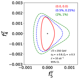
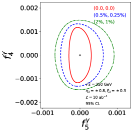
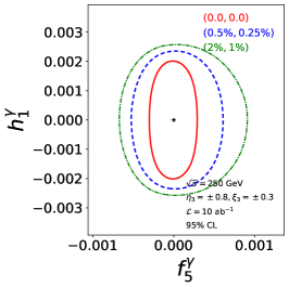
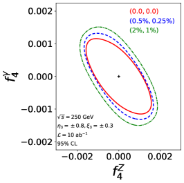
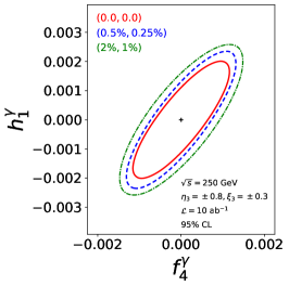
Figure 8: Two dimensional projections of marginalized anomalous couplings at 95%percent9595\% CL for varying systematic error and integrated luminosity of 10 ab-1.

IV Conclusion

In conclusion, we probe two processes viz. eāˆ’ā€‹e+ā†’Zā€‹Zā†’4ā€‹lā†’superscriptš‘’superscriptš‘’š‘š‘ā†’4š‘™e^{-}e^{+}\to ZZ\to 4l and eāˆ’ā€‹e+ā†’Zā€‹Ī³ā†’2ā€‹lā€‹Ī³ā†’superscriptš‘’superscriptš‘’š‘š›¾ā†’2š‘™š›¾e^{-}e^{+}\to Z\gamma\to 2l\gamma for upcoming International Linear ColliderĀ (ILC) at center of mass energy of 250250250Ā GeV with polarized beams in presence of four dimension-8 operators given in Eq.Ā (4). These operators generates anomalous neutral triple gauge couplingsĀ (Zā‹†ā€‹Zā€‹Z,Ī³ā‹†ā€‹Zā€‹Z,Ī³ā‹†ā€‹Zā€‹Ī³superscriptš‘ā‹†š‘š‘superscriptš›¾ā‹†š‘š‘superscriptš›¾ā‹†š‘š›¾Z^{\star}ZZ,\gamma^{\star}ZZ,\gamma^{\star}Z\gamma). To constrain the relevant Wilson coefficient, we construct polarization asymmetries of Zš‘Z boson in case of Zā€‹Ī³š‘š›¾Z\gamma and for Zā€‹Zš‘š‘ZZ additional spin correlation asymmetries were also constructed. These observables were further divided into eight bins of cosā”ĪøZsubscriptšœƒš‘\cos\theta_{Z}, where ĪøZsubscriptšœƒš‘\theta_{Z} is the angle between Zš‘Z boson and the beam axis in the lab frame. In case of Zā€‹Ī³š‘š›¾Z\gamma process, there exist eight asymmetries in each bin where five are CP-even and three are CP-odd. While for Zā€‹Zš‘š‘ZZ process there are 80 asymmetries in each bin out of which 44 are CP-even and 36 are CP-odd. These CP-odd observables can be used to measure CP-violation in the production process. We used all these asymmetries along with crossĀ section to put a simultaneous constrain on anomalous couplings using MCMC analysis. The final limits are obtained by combining Zā€‹Ī³š‘š›¾Z\gamma and Zā€‹Zš‘š‘ZZ process with two set of beam polarization at the level of Ļ‡2superscriptšœ’2\chi^{2}.
The limits on anomalous couplings cisubscriptš‘š‘–c_{i} except for cBā€‹Wsubscriptš‘šµš‘Šc_{BW} are dominated by the Zā€‹Ī³š‘š›¾Z\gamma process. The one parameter limits obtained in this work are tighter in the case of Zā€‹Zš‘š‘ZZ process, while for the Zā€‹Ī³š‘š›¾Z\gamma process, the limits are comparable to the LHC limits listed in TableĀ 1. The anomalous couplings contain momentum-dependent terms normalized by the electroweak scale, making them more prominent at higher energy. Analysis at LHC also enjoys higher crossĀ section for both Zā€‹Zš‘š‘ZZ and Zā€‹Ī³š‘š›¾Z\gamma process; thus, variable like crossĀ section alone provides significant sensitivity to anomalous couplings. Thus, using many observables like polarizations and spin correlations becomes necessary to compensate for the low energy and crossĀ section at ILC. Those observables could probe the CP structure of new physics. The current analysis could be extended by inculcating semi-leptonic and hadronic decay channels of Zš‘Z bosons.

Acknowledgements.
A. Subba acknowledge University Grant Commission, Govt. of India, New Delhi for financial support through UGC-NET Senior Research Fellowship.

Appendix A Anomalous couplings fiV,hiVsuperscriptsubscriptš‘“š‘–š‘‰superscriptsubscriptā„Žš‘–š‘‰f_{i}^{V},h_{i}^{V}

We use Eq.Ā (7 - 10) to obtain the marginalized limits on fiVsuperscriptsubscriptš‘“š‘–š‘‰f_{i}^{V}, and hiVsuperscriptsubscriptā„Žš‘–š‘‰h_{i}^{V} by MCMC global fits. We list the marginalized limits on four independent anomalous couplings in Table 4 for different values of luminosity and systematic errors. In order to understand the behaviour of the anomalous couplings in presence of varying systematic errors, we show the marginalized two dimensional projection of four independent anomalous couplings at 95%percent9595\% CL in Fig.Ā 8. The figures are obtained for different set of systematic errors and integrated luminosity of 10Ā fb-1. The confidence interval for f5Ī³superscriptsubscriptš‘“5š›¾f_{5}^{\gamma} improved by a factor of ā‰ˆ\approx 2.68 on decreasing the systematic from (2.0%,1.0%percent2.0percent1.02.0\%,1.0\%) to zero. While for the Cā€‹Pš¶š‘ƒCP-odd couplings, the confidence interval on f4Zsuperscriptsubscriptš‘“4š‘f_{4}^{Z} gets tighter by a factor of ā‰ˆ\approx 1.7 and similarly for f4Ī³,superscriptsubscriptš‘“4š›¾f_{4}^{\gamma}, and g1Ī³superscriptsubscriptš‘”1š›¾g_{1}^{\gamma} becomes better by a factor of ā‰ˆ\approx 1.3. The number suggest that the at the value of luminosity of 10Ā fb-1, the limits become blind to the systematic errors except in case of one Cā€‹Pš¶š‘ƒCP-even coupling. Similarly, if the luminosity increases by a factor of 100 while keeping the conservative value of systematic error, the limits on all the anomalous couplings gets better by a factor of approximately 3. The limits on these couplings can be probed to better precision with higher center of mass energy and increasing the polarization degree of positron which is one of the technological challenge for future electron-positron Collider.

Table 4: The translated marginalized 95%percent9595\% CL of anomalous couplingsĀ fiV,hiVsuperscriptsubscriptš‘“š‘–š‘‰superscriptsubscriptā„Žš‘–š‘‰f_{i}^{V},h_{i}^{V}Ā (10āˆ’3superscript10310^{-3}) at s=250š‘ 250\sqrt{s}=250 GeV with beam polarizationĀ (Ī·3,Ī¾3subscriptšœ‚3subscriptšœ‰3\eta_{3},\xi_{3}) = (Ā±0.8,Ā±0.3plus-or-minus0.8plus-or-minus0.3\pm 0.8,\pm 0.3) from MCMC global fits for different values of luminosities and systematic error.
ā„’ā„’\mathcal{L}Ā (fb-1) Ā Ā ā€ƒā€ƒ(ĻµĻƒ,ĻµA)subscriptitalic-ĻµšœŽsubscriptitalic-Ļµš“(\epsilon_{\sigma},\epsilon_{A}) Ā Ā ā€ƒā€ƒf5Ī³superscriptsubscriptš‘“5š›¾f_{5}^{\gamma} Ā Ā ā€ƒā€ƒf4Zsuperscriptsubscriptš‘“4š‘f_{4}^{Z} Ā Ā ā€ƒā€ƒf4Ī³superscriptsubscriptš‘“4š›¾f_{4}^{\gamma} Ā Ā ā€ƒā€ƒh1Ī³superscriptsubscriptā„Ž1š›¾h_{1}^{\gamma}
(0.0,0.0)0.00.0(0.0,0.0) Ā Ā ā€ƒā€ƒ[āˆ’1.43,+1.52]1.431.52[-1.43,+1.52] Ā Ā ā€ƒā€ƒ[āˆ’5.82,+5.50]5.825.50[-5.82,+5.50] Ā Ā ā€ƒā€ƒ[āˆ’3.68,+3.66]3.683.66[-3.68,+3.66] Ā Ā ā€ƒā€ƒ[āˆ’6.34,+6.26]6.346.26[-6.34,+6.26]
100 (0.5%,0.25%percent0.5percent0.250.5\%,0.25\%) Ā Ā ā€ƒā€ƒ[āˆ’1.45,+1.55]1.451.55[-1.45,+1.55] Ā Ā ā€ƒā€ƒ[āˆ’5.60,+5.52]5.605.52[-5.60,+5.52] Ā Ā ā€ƒā€ƒ[āˆ’3.68,+3.66]3.683.66[-3.68,+3.66] Ā Ā ā€ƒā€ƒ[āˆ’6.35,+6.27]6.356.27[-6.35,+6.27]
(2.0%,1.0%)percent2.0percent1.0(2.0\%,1.0\%) Ā Ā ā€ƒā€ƒ[āˆ’1.57,+1.72]1.571.72[-1.57,+1.72] Ā Ā ā€ƒā€ƒ[āˆ’5.69,+5.65]5.695.65[-5.69,+5.65] Ā Ā ā€ƒā€ƒ[āˆ’3.71,+3.67]3.713.67[-3.71,+3.67] Ā Ā ā€ƒā€ƒ[āˆ’6.43,+6.32]6.436.32[-6.43,+6.32]
(0.0,0.0)0.00.0(0.0,0.0) Ā Ā ā€ƒā€ƒ[āˆ’1.00,+1.05]1.001.05[-1.00,+1.05] Ā Ā ā€ƒā€ƒ[āˆ’4.10,+4.06]4.104.06[-4.10,+4.06] Ā Ā ā€ƒā€ƒ[āˆ’2.77,+2.77]2.772.77[-2.77,+2.77] Ā Ā ā€ƒā€ƒ[āˆ’4.72,+4.71]4.724.71[-4.72,+4.71]
300300300 (0.5%,0.25%)percent0.5percent0.25(0.5\%,0.25\%) Ā Ā ā€ƒā€ƒ[āˆ’1.05,+1.12]1.051.12[-1.05,+1.12] Ā Ā ā€ƒā€ƒ[āˆ’4.12,+4.10]4.124.10[-4.12,+4.10] Ā Ā ā€ƒā€ƒ[āˆ’2.79,+2.79]2.792.79[-2.79,+2.79] Ā Ā ā€ƒā€ƒ[āˆ’4.77,+4.75]4.774.75[-4.77,+4.75]
(2.0%,1.0%)percent2.0percent1.0(2.0\%,1.0\%) Ā Ā ā€ƒā€ƒ[āˆ’1.22,+1.38]1.221.38[-1.22,+1.38] Ā Ā ā€ƒā€ƒ[āˆ’4.26,+4.24]4.264.24[-4.26,+4.24] Ā Ā ā€ƒā€ƒ[āˆ’2.81,+2.81]2.812.81[-2.81,+2.81] Ā Ā ā€ƒā€ƒ[āˆ’4.87,+4.84]4.874.84[-4.87,+4.84]
(0.0,0.0)0.00.0(0.0,0.0) Ā Ā ā€ƒā€ƒ[āˆ’0.65,+0.66]0.650.66[-0.65,+0.66] Ā Ā ā€ƒā€ƒ[āˆ’2.87,+2.86]2.872.86[-2.87,+2.86] Ā Ā ā€ƒā€ƒ[āˆ’1.99,+2.01]1.992.01[-1.99,+2.01] Ā Ā ā€ƒā€ƒ[āˆ’3.38,+3.38]3.383.38[-3.38,+3.38]
1000 (0.5%,0.25%)percent0.5percent0.25(0.5\%,0.25\%) Ā Ā ā€ƒā€ƒ[āˆ’0.74,+0.80]0.740.80[-0.74,+0.80] Ā Ā ā€ƒā€ƒ[āˆ’2.91,+2.90]2.912.90[-2.91,+2.90] Ā Ā ā€ƒā€ƒ[āˆ’2.02,+2.03]2.022.03[-2.02,+2.03] Ā Ā ā€ƒā€ƒ[āˆ’3.47,+3.46]3.473.46[-3.47,+3.46]
(2.0%,1.0%)percent2.0percent1.0(2.0\%,1.0\%) Ā Ā ā€ƒā€ƒ[āˆ’0.92,+1.12]0.921.12[-0.92,+1.12] Ā Ā ā€ƒā€ƒ[āˆ’3.05,+3.04]3.053.04[-3.05,+3.04] Ā Ā ā€ƒā€ƒ[āˆ’2.07,+2.08]2.072.08[-2.07,+2.08] Ā Ā ā€ƒā€ƒ[āˆ’3.60,+3.60]3.603.60[-3.60,+3.60]
(0.0,0.0)0.00.0(0.0,0.0) Ā Ā ā€ƒā€ƒ[āˆ’0.42,+0.41]0.420.41[-0.42,+0.41] Ā Ā ā€ƒā€ƒ[āˆ’2.02,+2.00]2.022.00[-2.02,+2.00] Ā Ā ā€ƒā€ƒ[āˆ’1.44,+1.45]1.441.45[-1.44,+1.45] Ā Ā ā€ƒā€ƒ[āˆ’2.44,+2.44]2.442.44[-2.44,+2.44]
3000 (0.5%,0.25%)percent0.5percent0.25(0.5\%,0.25\%) Ā Ā ā€ƒā€ƒ[āˆ’0.56,+0.63]0.560.63[-0.56,+0.63] Ā Ā ā€ƒā€ƒ[āˆ’2.07,+2.06]2.072.06[-2.07,+2.06] Ā Ā ā€ƒā€ƒ[āˆ’1.50,+1.51]1.501.51[-1.50,+1.51] Ā Ā ā€ƒā€ƒ[āˆ’2.61,+2.61]2.612.61[-2.61,+2.61]
(2.0%,1.0%)percent2.0percent1.0(2.0\%,1.0\%) Ā Ā ā€ƒā€ƒ[āˆ’0.74,+0.08]0.740.08[-0.74,+0.08] Ā Ā ā€ƒā€ƒ[āˆ’2.18,+2.18]2.182.18[-2.18,+2.18] Ā Ā ā€ƒā€ƒ[āˆ’1.58,+1.59]1.581.59[-1.58,+1.59] Ā Ā ā€ƒā€ƒ[āˆ’2.76,+2.76]2.762.76[-2.76,+2.76]
(0.0,0.0)0.00.0(0.0,0.0) Ā Ā ā€ƒā€ƒ[āˆ’0.25,+0.24]0.250.24[-0.25,+0.24] Ā Ā ā€ƒā€ƒ[āˆ’1.29,+1.27]1.291.27[-1.29,+1.27] Ā Ā ā€ƒā€ƒ[āˆ’0.94,+0.95]0.940.95[-0.94,+0.95] Ā Ā ā€ƒā€ƒ[āˆ’1.64,+1.65]1.641.65[-1.64,+1.65]
10000 (0.5%,0.25%)percent0.5percent0.25(0.5\%,0.25\%) Ā Ā ā€ƒā€ƒ[āˆ’0.44,+0.50]0.440.50[-0.44,+0.50] Ā Ā ā€ƒā€ƒ[āˆ’1.35,+1.35]1.351.35[-1.35,+1.35] Ā Ā ā€ƒā€ƒ[āˆ’1.08,+1.08]1.081.08[-1.08,+1.08] Ā Ā ā€ƒā€ƒ[āˆ’1.94,+1,94]1.94194[-1.94,+1,94]
(2.0%,1.0%)percent2.0percent1.0(2.0\%,1.0\%) Ā Ā ā€ƒā€ƒ[āˆ’0.57,+0.74]0.570.74[-0.57,+0.74] Ā Ā ā€ƒā€ƒ[āˆ’1.51,+1.50]1.511.50[-1.51,+1.50] Ā Ā ā€ƒā€ƒ[āˆ’1.22,+1.23]1.221.23[-1.22,+1.23] Ā Ā ā€ƒā€ƒ[āˆ’2.14,+2.14]2.142.14[-2.14,+2.14]

References

  • AadĀ etĀ al. [2012a] G.Ā Aad etĀ al. (ATLAS),Ā Observation of a new particle in the search for the Standard Model Higgs boson with the ATLAS detector at the LHC,Ā Phys. Lett. BĀ 716,Ā 1 (2012a),Ā arXiv:1207.7214 [hep-ex] .
  • ChatrchyanĀ etĀ al. [2012] S.Ā Chatrchyan etĀ al. (CMS),Ā Observation of a New Boson at a Mass of 125 GeV with the CMS Experiment at the LHC,Ā Phys. Lett. BĀ 716,Ā 30 (2012),Ā arXiv:1207.7235 [hep-ex] .
  • AdeĀ etĀ al. [2014] P.Ā A.Ā R.Ā Ade etĀ al. (Planck),Ā Planck 2013 results. XVI. Cosmological parameters,Ā Astron. Astrophys.Ā 571,Ā A16 (2014),Ā arXiv:1303.5076 [astro-ph.CO] .
  • AaltonenĀ etĀ al. [2022] T.Ā Aaltonen etĀ al. (CDF),Ā High-precision measurement of the Wš‘ŠW boson mass with the CDF II detector,Ā ScienceĀ 376,Ā 170 (2022).
  • AbiĀ etĀ al. [2021] B.Ā Abi etĀ al. (Muon g-2),Ā Measurement of the Positive Muon Anomalous Magnetic Moment to 0.46 ppm,Ā Phys. Rev. Lett.Ā 126,Ā 141801 (2021),Ā arXiv:2104.03281 [hep-ex] .
  • Georgi [1993] H.Ā Georgi,Ā Effective field theory,Ā Ann. Rev. Nucl. Part. Sci.Ā 43,Ā 209 (1993).
  • Weinberg [1979] S.Ā Weinberg,Ā Phenomenological Lagrangians,Ā Physica AĀ 96,Ā 327 (1979).
  • Weinberg [1980] S.Ā Weinberg,Ā Effective Gauge Theories,Ā Phys. Lett. BĀ 91,Ā 51 (1980).
  • Degrande [2014] C.Ā Degrande,Ā A basis of dimension-eight operators for anomalous neutral triple gauge boson interactions,Ā JHEPĀ 02,Ā 101,Ā arXiv:1308.6323 [hep-ph] .
  • HagiwaraĀ etĀ al. [1987] K.Ā Hagiwara, R.Ā D.Ā Peccei, D.Ā Zeppenfeld,Ā andĀ K.Ā Hikasa,Ā Probing the Weak Boson Sector in e+ e- ā€”>> W+ W-,Ā Nucl. Phys. BĀ 282,Ā 253 (1987).
  • GounarisĀ etĀ al. [2000] G.Ā J.Ā Gounaris, J.Ā Layssac,Ā andĀ F.Ā M.Ā Renard,Ā Signatures of the anomalous ZĪ³subscriptš‘š›¾Z_{\gamma} and Zā€‹Zš‘š‘ZZ production at the lepton and hadron colliders,Ā Phys. Rev. DĀ 61,Ā 073013 (2000),Ā arXiv:hep-ph/9910395 .
  • AcciarriĀ etĀ al. [1999] M.Ā Acciarri etĀ al. (L3),Ā Study of Zš‘Z Boson Pair Production in e+ā€‹eāˆ’superscriptš‘’superscriptš‘’e^{+}e^{-} collisions at LEP at S(1/2)superscriptš‘†12S^{(1/2)} = 189-GeV,Ā Phys. Lett. BĀ 465,Ā 363 (1999),Ā arXiv:hep-ex/9909043 .
  • AbbiendiĀ etĀ al. [2003] G.Ā Abbiendi etĀ al. (OPAL),Ā Study of Z pair production and anomalous couplings in e+ e- collisions at s**(1/2) between 190-GeV and 209-GeV,Ā Eur. Phys. J. CĀ 32,Ā 303 (2003),Ā arXiv:hep-ex/0310013 .
  • AlcarazĀ etĀ al. [2006] J.Ā Alcaraz etĀ al. (ALEPH, DELPHI, L3, OPAL, LEP Electroweak Working Group),Ā A Combination of preliminary electroweak measurements and constraints on the standard model,Ā Ā  (2006),Ā arXiv:hep-ex/0612034 .
  • ChatrchyanĀ etĀ al. [2013] S.Ā Chatrchyan etĀ al. (CMS),Ā Measurement of the Zā€‹Zš‘š‘ZZ Production Cross Section and Search for Anomalous Couplings in 2 l2l ā€™ Final States in pā€‹pš‘š‘pp Collisions at s=7š‘ 7\sqrt{s}=7 TeV,Ā JHEPĀ 01,Ā 063,Ā arXiv:1211.4890 [hep-ex] .
  • AadĀ etĀ al. [2012b] G.Ā Aad etĀ al. (ATLAS),Ā Measurement of Wā€‹Ī³š‘Šš›¾W\gamma and Zā€‹Ī³š‘š›¾Z\gamma production cross sections in pā€‹pš‘š‘pp collisions at s=7š‘ 7\sqrt{s}=7 TeV and limits on anomalous triple gauge couplings with the ATLAS detector,Ā Phys. Lett. BĀ 717,Ā 49 (2012b),Ā arXiv:1205.2531 [hep-ex] .
  • Collaboration [2023] A.Ā Collaboration,Ā Evidence of pair production of longitudinally polarised vector bosons and study of cp properties in zā€‹zā†’4ā€‹ā„“ā†’š‘§š‘§4ā„“zz\to 4\ell events with the atlas detector at s=13š‘ 13\sqrt{s}=13 tev,Ā Ā  (2023),Ā arXiv:2310.04350 [hep-ex] .
  • AbazovĀ etĀ al. [2008] V.Ā M.Ā Abazov etĀ al. (D0),Ā Search for Zā€‹Zš‘š‘ZZ and Zā€‹Ī³āˆ—š‘superscriptš›¾Z\gamma^{*} production in pā€‹pĀÆš‘ĀÆš‘p\bar{p} collisions at sš‘ \sqrt{s} = 1.96 TeV and limits on anomalous Zā€‹Zā€‹Zš‘š‘š‘ZZZ and Zā€‹Zā€‹Ī³āˆ—š‘š‘superscriptš›¾ZZ\gamma^{*} couplings,Ā Phys. Rev. Lett.Ā 100,Ā 131801 (2008),Ā arXiv:0712.0599 [hep-ex] .
  • AaltonenĀ etĀ al. [2012] T.Ā Aaltonen etĀ al. (CDF),Ā Measurement of Zā€‹Zš‘š‘ZZ production in leptonic final states at sš‘ \surd{s} of 1.96 TeV at CDF,Ā Phys. Rev. Lett.Ā 108,Ā 101801 (2012),Ā arXiv:1112.2978 [hep-ex] .
  • DegrandeĀ etĀ al. [2012] C.Ā Degrande, C.Ā Duhr, B.Ā Fuks, D.Ā Grellscheid, O.Ā Mattelaer,Ā andĀ T.Ā Reiter,Ā UFO - The Universal FeynRules Output,Ā Comput. Phys. Commun.Ā 183,Ā 1201 (2012),Ā arXiv:1108.2040 [hep-ph] .
  • AlloulĀ etĀ al. [2014] A.Ā Alloul, N.Ā D.Ā Christensen, C.Ā Degrande, C.Ā Duhr,Ā andĀ B.Ā Fuks,Ā FeynRules 2.0 - A complete toolbox for tree-level phenomenology,Ā Comput. Phys. Commun.Ā 185,Ā 2250 (2014),Ā arXiv:1310.1921 [hep-ph] .
  • AlwallĀ etĀ al. [2011] J.Ā Alwall, M.Ā Herquet, F.Ā Maltoni, O.Ā Mattelaer,Ā andĀ T.Ā Stelzer,Ā MadGraph 5 : Going Beyond,Ā JHEPĀ 06,Ā 128,Ā arXiv:1106.0522 [hep-ph] .
  • AlwallĀ etĀ al. [2014] J.Ā Alwall, R.Ā Frederix, S.Ā Frixione, V.Ā Hirschi, F.Ā Maltoni, O.Ā Mattelaer, H.Ā S.Ā Shao, T.Ā Stelzer, P.Ā Torrielli,Ā andĀ M.Ā Zaro,Ā The automated computation of tree-level and next-to-leading order differential cross sections, and their matching to parton shower simulations,Ā JHEPĀ 07,Ā 079,Ā arXiv:1405.0301 [hep-ph] .
  • SubbaĀ andĀ Singh [2023a] A.Ā SubbaĀ andĀ R.Ā K.Ā Singh,Ā Role of polarizations and spin-spin correlations of Wā€™s in e-e+ā†’W-W+ at s=250ā€‰ā€‰GeV to probe anomalous W-W+Z/Ī³š›¾\gamma couplings,Ā Phys. Rev. DĀ 107,Ā 073004 (2023a),Ā arXiv:2212.12973 [hep-ph] .
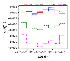
  • RahamanĀ andĀ Singh [2016] R.Ā RahamanĀ andĀ R.Ā K.Ā Singh,Ā On polarization parameters of spin-1 particles and anomalous couplings in e+ā€‹eāˆ’ā†’Zā€‹Z/Zā€‹Ī³ā†’superscriptš‘’superscriptš‘’š‘š‘š‘š›¾e^{+}e^{-}\rightarrow ZZ/Z\gamma,Ā Eur. Phys. J. CĀ 76,Ā 539 (2016),Ā arXiv:1604.06677 [hep-ph] .
  • RahamanĀ andĀ Singh [2017] R.Ā RahamanĀ andĀ R.Ā K.Ā Singh,Ā On the choice of beam polarization in e+ā€‹eāˆ’ā†’Zā€‹Z/Zā€‹Ī³ā†’superscriptš‘’superscriptš‘’š‘š‘š‘š›¾e^{+}e^{-}\rightarrow ZZ/Z\gamma and anomalous triple gauge-boson couplings,Ā Eur. Phys. J. CĀ 77,Ā 521 (2017),Ā arXiv:1703.06437 [hep-ph] .
  • ILC [2013] The International Linear Collider Technical Design Report - Volume 2: Physics,Ā Ā  (2013),Ā arXiv:1306.6352 [hep-ph] .
  • Ado [2013] The International Linear Collider Technical Design Report - Volume 3.II: Accelerator Baseline Design,Ā Ā  (2013),Ā arXiv:1306.6328 [physics.acc-ph] .
  • CharlesĀ etĀ al. [2018] T.Ā K.Ā Charles etĀ al. (CLICdp, CLIC),Ā The Compact Linear Collider (CLIC) - 2018 Summary ReportĀ 2/2018,Ā 10.23731/CYRM-2018-002 (2018),Ā arXiv:1812.06018 [physics.acc-ph] .
  • AbadaĀ etĀ al. [2019] A.Ā Abada etĀ al. (FCC),Ā FCC-ee: The Lepton Collider: Future Circular Collider Conceptual Design Report Volume 2,Ā Eur. Phys. J. STĀ 228,Ā 261 (2019).
  • DemirciĀ andĀ Balantekin [2022] M.Ā DemirciĀ andĀ A.Ā B.Ā Balantekin,Ā Beam polarization effects on Z-boson pair production at electron-positron colliders: A full one-loop analysis,Ā Phys. Rev. DĀ 106,Ā 073003 (2022),Ā arXiv:2209.13720 [hep-ph] .
  • Swartz [1987] M.Ā L.Ā Swartz,Ā PHYSICS WITH POLARIZED ELECTRON BEAMS,Ā Conf. Proc. CĀ 8708101,Ā 83 (1987).
  • ChenĀ etĀ al. [2022] S.Ā H.Ā Chen etĀ al.,Ā A toy Monte Carlo simulation for the transverse polarization of high-energy electron beams,Ā JINSTĀ 17 (08),Ā P08005.
  • Hikasa [1984] K.-i.Ā Hikasa,Ā Effects of Transverse Polarization in Electron - Positron Collisions,Ā Phys. Lett. BĀ 143,Ā 266 (1984).
  • Hikasa [1986] K.-i.Ā Hikasa,Ā Transverse Polarization Effects in e+ā€‹eāˆ’superscriptš‘’superscriptš‘’e^{+}e^{-} Collisions: The Role of Chiral Symmetry,Ā Phys. Rev. DĀ 33,Ā 3203 (1986).
  • Renard [1989] F.Ā M.Ā Renard,Ā Single Transverse Polarization Effects in e+ā€‹eāˆ’superscriptš‘’superscriptš‘’e^{+}e^{-} Collisions and the Structure of Chirality Violation,Ā Z. Phys. CĀ 45,Ā 75 (1989).
  • WenĀ etĀ al. [2023] X.-K.Ā Wen, B.Ā Yan, Z.Ā Yu,Ā andĀ C.Ā P.Ā Yuan,Ā Single Transverse Spin Asymmetry as a New Probe of Standard-Model-Effective-Field-Theory Dipole Operators,Ā Phys. Rev. Lett.Ā 131,Ā 241801 (2023),Ā arXiv:2307.05236 [hep-ph] .
  • PlacidiĀ andĀ Rossmanith [1985] M.Ā PlacidiĀ andĀ R.Ā Rossmanith,Ā TRANSVERSE AND LONGITUDINAL POLARIZATION IN LEP,Ā inĀ Conference on Tests of Electroweak Theories: Polarized Processes and Other PhenomenaĀ (1985).
  • BarateĀ etĀ al. [1999] R.Ā Barate etĀ al. (ALEPH),Ā Measurement of the e+ e- ā€”>> Z Z production cross-section at center-of-mass energies of 183-GeV and 189-GeV,Ā Phys. Lett. BĀ 469,Ā 287 (1999),Ā arXiv:hep-ex/9911003 .
  • SchaelĀ etĀ al. [2013] S.Ā Schael etĀ al. (ALEPH, DELPHI, L3, OPAL, LEP Electroweak),Ā Electroweak Measurements in Electron-Positron Collisions at W-Boson-Pair Energies at LEP,Ā Phys. Rept.Ā 532,Ā 119 (2013),Ā arXiv:1302.3415 [hep-ex] .
  • AbdallahĀ etĀ al. [2003] J.Ā Abdallah etĀ al. (DELPHI),Ā ZZ production in e+ e- interactions at s**(1/2) = 183-GeV to 209-GeV,Ā Eur. Phys. J. CĀ 30,Ā 447 (2003),Ā arXiv:hep-ex/0307050 .
  • AaltonenĀ etĀ al. [2014] T.Ā A.Ā Aaltonen etĀ al. (CDF),Ā Measurement of the ZZ production cross section using the full CDF II data set,Ā Phys. Rev. DĀ 89,Ā 112001 (2014),Ā arXiv:1403.2300 [hep-ex] .
  • AbazovĀ etĀ al. [2013] V.Ā M.Ā Abazov etĀ al. (D0),Ā Measurement of the ZZ production cross section and search for the standard model Higgs boson in the four lepton final state in ppbar collisions,Ā Phys. Rev. DĀ 88,Ā 032008 (2013),Ā arXiv:1304.5422 [hep-ex] .
  • AaboudĀ etĀ al. [2018a] M.Ā Aaboud etĀ al. (ATLAS),Ā Zā€‹Zā†’ā„“+ā€‹ā„“āˆ’ā€‹ā„“ā€²ā£+ā€‹ā„“ā€²ā£āˆ’ā†’š‘š‘superscriptā„“superscriptā„“superscriptā„“ā€²superscriptā„“ā€²ZZ\to\ell^{+}\ell^{-}\ell^{\prime+}\ell^{\prime-} cross-section measurements and search for anomalous triple gauge couplings in 13 TeV pā€‹pš‘š‘pp collisions with the ATLAS detector,Ā Phys. Rev. DĀ 97,Ā 032005 (2018a),Ā arXiv:1709.07703 [hep-ex] .
  • AaboudĀ etĀ al. [2018b] M.Ā Aaboud etĀ al. (ATLAS),Ā Measurement of the Zā€‹Ī³ā†’Ī½ā€‹Ī½ĀÆā€‹Ī³ā†’š‘š›¾šœˆĀÆšœˆš›¾Z\gamma\to\nu\overline{\nu}\gamma production cross section in pp collisions at s=13š‘ 13\sqrt{s}=13 TeV with the ATLAS detector and limits on anomalous triple gauge-boson couplings,Ā JHEPĀ 12,Ā 010,Ā arXiv:1810.04995 [hep-ex] .
  • SirunyanĀ etĀ al. [2018] A.Ā M.Ā Sirunyan etĀ al. (CMS),Ā Measurements of the ppā†’ZZā†’ppZZ\mathrm{p}\mathrm{p}\rightarrow\mathrm{Z}\mathrm{Z} production cross section and the Zā†’4ā€‹ā„“ā†’Z4ā„“\mathrm{Z}\rightarrow 4\ell branching fraction, and constraints on anomalous triple gauge couplings at s=13ā€‹TeVš‘ 13TeV\sqrt{s}=13\,\text{TeV},Ā Eur. Phys. J. CĀ 78,Ā 165 (2018),Ā [Erratum: Eur.Phys.J.C 78, 515 (2018)],Ā arXiv:1709.08601 [hep-ex] .
  • YilmazĀ etĀ al. [2020] A.Ā Yilmaz, A.Ā Senol, H.Ā Denizli, I.Ā TurkĀ Cakir,Ā andĀ O.Ā Cakir,Ā Sensitivity on Anomalous Neutral Triple Gauge Couplings via Zā€‹Zš‘š‘ZZ Production at FCC-hh,Ā Eur. Phys. J. CĀ 80,Ā 173 (2020),Ā arXiv:1906.03911 [hep-ph] .
  • SenolĀ etĀ al. [2018] A.Ā Senol, H.Ā Denizli, A.Ā Yilmaz, I.Ā TurkĀ Cakir, K.Ā Y.Ā Oyulmaz, O.Ā Karadeniz,Ā andĀ O.Ā Cakir,Ā Probing the Effects of Dimension-eight Operators Describing Anomalous Neutral Triple Gauge Boson Interactions at FCC-hh,Ā Nucl. Phys. BĀ 935,Ā 365 (2018),Ā arXiv:1805.03475 [hep-ph] .
  • Spor [2023] S.Ā Spor,Ā Probe of the anomalous neutral triple gauge couplings in photon-induced collision at future muon colliders,Ā Nucl. Phys. BĀ 991,Ā 116198 (2023),Ā arXiv:2207.11585 [hep-ph] .
  • JahediĀ andĀ Lahiri [2023] S.Ā JahediĀ andĀ J.Ā Lahiri,Ā Probing anomalous ZZĪ³š›¾\gamma and ZĪ³š›¾\gammaĪ³š›¾\gamma couplings at the e+e- colliders using optimal observable technique,Ā JHEPĀ 04,Ā 085,Ā arXiv:2212.05121 [hep-ph] .
  • AtagĀ andĀ Sahin [2004] S.Ā AtagĀ andĀ I.Ā Sahin,Ā ZZ gamma and Z gamma gamma couplings at linear e+ e- collider energies with the effects of Z polarization and initial state radiation,Ā Phys. Rev. DĀ 70,Ā 053014 (2004),Ā arXiv:hep-ph/0408163 .
  • OtsĀ etĀ al. [2004] I.Ā Ots, H.Ā Uibo, H.Ā Liivat, R.Ā Saar,Ā andĀ R.Ā K.Ā Loide,Ā Possible anomalous Z Z gamma and Z gamma gamma couplings and Z boson spin orientation in e+ e- ā€”>> Z gamma,Ā Nucl. Phys. BĀ 702,Ā 346 (2004).
  • Gutierrez-RodriguezĀ etĀ al. [2009] A.Ā Gutierrez-Rodriguez, M.Ā A.Ā Hernandez-Ruiz,Ā andĀ M.Ā A.Ā Perez,Ā Probing the ZZgamma and Z gamma gamma Couplings Through the Process e+ e- ā€”>> nu anti-nu gamma,Ā Phys. Rev. DĀ 80,Ā 017301 (2009),Ā arXiv:0808.0945 [hep-ph] .
  • EllisĀ etĀ al. [2020] J.Ā Ellis, S.-F.Ā Ge, H.-J.Ā He,Ā andĀ R.-Q.Ā Xiao,Ā Probing the scale of new physics in the Zā€‹Zā€‹Ī³š‘š‘š›¾ZZ\gamma coupling at e+ā€‹eāˆ’superscriptš‘’superscriptš‘’e^{+}e^{-} colliders,Ā Chin. Phys. CĀ 44,Ā 063106 (2020),Ā arXiv:1902.06631 [hep-ph] .
  • SenolĀ etĀ al. [2020] A.Ā Senol, H.Ā Denizli, A.Ā Yilmaz, I.Ā TurkĀ Cakir,Ā andĀ O.Ā Cakir,Ā The projections on Zā€‹Zā€‹Ī³š‘š‘š›¾ZZ\gamma and Zā€‹Ī³ā€‹Ī³š‘š›¾š›¾Z\gamma\gamma couplings via Ī½ā€‹Ī½ĀÆā€‹Ī³šœˆĀÆšœˆš›¾\nu\bar{\nu}\gamma production in HL-LHC and HE-LHC,Ā Phys. Lett. BĀ 802,Ā 135255 (2020),Ā arXiv:1910.03843 [hep-ph] .
  • EllisĀ etĀ al. [2023] J.Ā Ellis, H.-J.Ā He,Ā andĀ R.-Q.Ā Xiao,Ā Probing neutral triple gauge couplings at the LHC and future hadron colliders,Ā Phys. Rev. DĀ 107,Ā 035005 (2023),Ā arXiv:2206.11676 [hep-ph] .
  • HernĆ”ndez-JuĆ”rezĀ etĀ al. [2021] A.Ā I.Ā HernĆ”ndez-JuĆ”rez, A.Ā Moyotl,Ā andĀ G.Ā Tavares-Velasco,Ā Contributions to Zā€‹Zā€‹Vāˆ—š‘š‘superscriptš‘‰ZZV^{*} (V=Ī³,Z,Zā€²š‘‰š›¾š‘superscriptš‘ā€²V=\gamma,Z,Z^{\prime}) couplings from Cā€‹Pš¶š‘ƒCP violating flavor changing couplings,Ā Eur. Phys. J. CĀ 81,Ā 304 (2021),Ā arXiv:2102.02197 [hep-ph] .
  • HernĆ”ndez-JuĆ”rezĀ andĀ Tavares-Velasco [2022] A.Ā I.Ā HernĆ”ndez-JuĆ”rezĀ andĀ G.Ā Tavares-Velasco,Ā Non-diagonal contributions to Zā€‹Ī³ā€‹Vāˆ—š‘š›¾superscriptš‘‰āˆ—Z\gamma V^{\ast} vertex and bounds on Zā€‹tĀÆā€‹qš‘ĀÆš‘”š‘žZ\overline{t}q couplings,Ā Ā  (2022),Ā arXiv:2203.16819 [hep-ph] .
  • RahamanĀ andĀ Singh [2019] R.Ā RahamanĀ andĀ R.Ā K.Ā Singh,Ā Anomalous triple gauge boson couplings in Zā€‹Zš‘š‘ZZ production at the LHC and the role of Zš‘Z boson polarizations,Ā Nucl. Phys. BĀ 948,Ā 114754 (2019),Ā arXiv:1810.11657 [hep-ph] .
  • BoudjemaĀ andĀ Singh [2009] F.Ā BoudjemaĀ andĀ R.Ā K.Ā Singh,Ā A Model independent spin analysis of fundamental particles using azimuthal asymmetries,Ā JHEPĀ 07,Ā 028,Ā arXiv:0903.4705 [hep-ph] .
  • RahamanĀ andĀ Singh [2022] R.Ā RahamanĀ andĀ R.Ā K.Ā Singh,Ā Breaking down the entire spectrum of spin correlations of a pair of particles involving fermions and gauge bosons,Ā Nucl. Phys. BĀ 984,Ā 115984 (2022),Ā arXiv:2109.09345 [hep-ph] .
  • RahamanĀ andĀ Singh [2020] R.Ā RahamanĀ andĀ R.Ā K.Ā Singh,Ā Probing the anomalous triple gauge boson couplings in e+ā€‹eāˆ’ā†’W+ā€‹Wāˆ’ā†’superscriptš‘’superscriptš‘’superscriptš‘Šsuperscriptš‘Še^{+}e^{-}\to W^{+}W^{-} using Wš‘ŠW polarizations with polarized beams,Ā Phys. Rev. DĀ 101,Ā 075044 (2020),Ā arXiv:1909.05496 [hep-ph] .
  • SubbaĀ andĀ Singh [2023b] A.Ā SubbaĀ andĀ R.Ā K.Ā Singh,Ā Study of anomalous Wāˆ’ā€‹W+ā€‹Ī³/Zsuperscriptš‘Šsuperscriptš‘Šš›¾š‘W^{-}W^{+}\gamma/Z couplings using polarizations and spin correlations in eāˆ’ā€‹e+ā†’Wāˆ’ā€‹W+ā†’superscriptš‘’superscriptš‘’superscriptš‘Šsuperscriptš‘Še^{-}e^{+}\to W^{-}W^{+} with polarized beams,Ā Ā  (2023b),Ā arXiv:2305.15106 [hep-ph] .