Optimal Investment and Fair Sharing Rules of the Incentives
for Renewable Energy Communities

Abstract

The focus on Renewable Energy Communities (REC) is fastly growing after the European Union (EU) has introduced a dedicated regulation in 2018. The idea of creating local groups of citizens, small- and medium-sized companies, and public institutions, which self-produce and self-consume energy from renewable sources is at the same time a way to save money for the participants, increase efficiency of the energy system, and reduce CO2 emissions.

Member states inside the EU are fixing more detailed regulations, which describe, among other things, how public incentives are measured. A natural objective for the incentive policies is of course to promote the self-consumption of a REC. A quite sophisticated incentive policy is that based on the so called ’virtual framework’ (which opposes to the ’physical’ one) as e.g. the one introduced in the Italian electricity market in 2019. Under this framework all the energy produced by a REC is sold to the market, and all the energy consumed must be paid to retailers: self-consumption occurs only ’virtually’, thanks a money compensation (paid by a central authority) for every MWh produced and consumed by the REC in the same hour. In this context, two relevant problems have to be solved: the optimal investment in new technologies and a fair division of the incentive among the community members. The two problems are clearly linked: an unfair sharing rule can jeopardize the profitability and the decision to invest and join a REC for some members.

We address these two problems by considering a particular type of REC, composed by a representative household and a biogas producer, where the potential demand of the community is given by the household’s demand, while both members produce renewable energy. Such a type of REC could be a typical case both in rural and urban areas. We assume that the biogas producer decides to install new technologies in order to transform the biogas into electricity and sell it in the electricity market at the spot price, whereas the biogas that is not transformed into energy can be sold on the gas market at the spot price. On one hand, we suppose that the household decides to install photovoltaic panels in order to partially cover its own power demand, thus reducing the purchase of energy in the market. On the other hand, investing in a renewable energy plant provides the household with the revenues of selling the energy exceeding its self-consumption. The relevant advantage of entering into a REC for both players is that their joint self-consumption is rewarded with a governmental incentive, which must be fairly shared.

We set the problem as a leader-follower problem: the leader decide how to share the incentive for the self-consumed energy, while the followers decide their own optimal installation strategy. We solve the leader’s problem by searching for a Nash bargaining solution for the incentive’s fair division, while the follower problem is solved by finding the Nash equilibria of a static competitive game between the members.

1 Introduction

The global problem of climate change and the process of energy transition is an unprecedented challenge for humanity. The possible solutions are different and involve all the segments of our societies. A potentially powerful solution aiming to reduce the emissions of CO₂ is that of sustaining final consumers to turn into self-producers and self-consumers of electricity generated through Renewable Energy Sources (RES). On this line, the EU has introduced two relatively recent directives (directive (EU) 2018/2001 [3] and directive (EU) 2019/944 [4]), which set the rules to allow private households, small enterprises, and local public authorities to join local Renewable Energy Communities (REC) with the purpose of sharing the generation of their renewable energy plants. Diversified self-consumption profiles within (relatively) small groups are expected to reduce grid congestion and improve overall efficiency of national energy systems. The introduction of such entities within national energy systems is intuitively delicate since they can significantly modify both the energy-mix of a country and the economic balance of the institutional players (i.e., generators, distributors, and retailers).

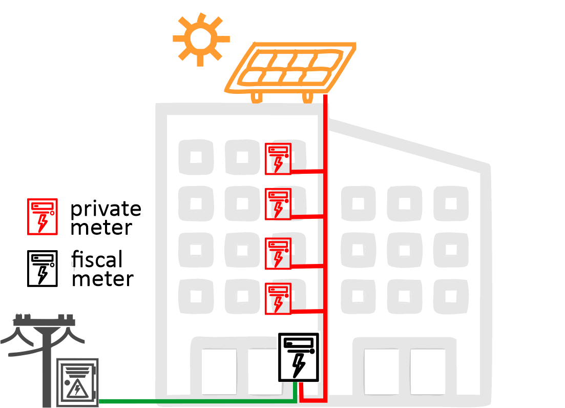
(a) Physical framework

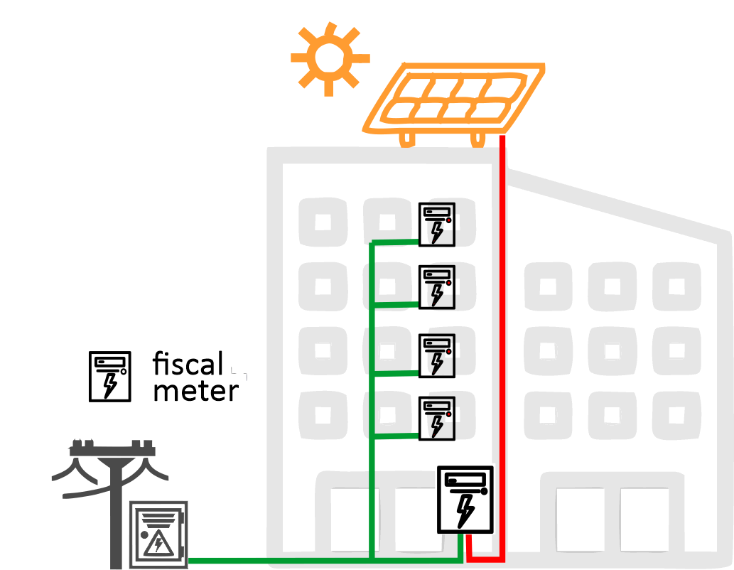
(b) Virtual framework

Figure 1: Difference between physical and virtual REC frameworks

The implementation of the EU directives across the Member States is occurring at different speeds. One of the first examples of implementation is that of Italy, which fixes a compensation mechanism that has chances to be replicated by other countries in the following years. In particular, the Italian regulation ([5, 6, 7]) introduces a quite sophisticated “virtual” self-consumption framework, to be conceptually opposed to the “physical” one. In the EU, 450 million people live and in 2020 they generated more than 3 trillion KWh over the 10 total OECD countries [12]. Italy is the first EU country to propose its own legislation for energy communities. The pioneering action of Italy, could influence and inspire other EU countries which aim to employ REC for energy transition.

Figure 1 shows the difference between the physical and the virtual frameworks, using as an example the smallest case of REC: a group of households in the same building. Adopting the physical framework 1(a), all households can consume directly the self-generated energy, and individual consumption is measured through private meters. The excess demand and excess generation are measured by a common fiscal meter and generate corresponding collective revenues / cost which are split among the members. According to the virtual framework 1(b), the members of a REC do not directly consume the energy generated with their plants (with the exception of some minor cases). Under the virtual scheme, all the generation of a REC must be offered to the market. Since the REC are going to be very small in size, a central authority (e.g., GSE in Italy, which acts as guarantor and promoter of the country’s sustainable development) is established as a natural broker, guaranteeing a selling price calculated as an average of the gross price of electricity updated periodically. To satisfy their energy needs, the members entering a REC must, therefore, continue to buy electricity from their retailers, their consumption remaining under the control of fiscal meters. This is why, for them, self-consumption occurs only in a virtual way, that is by offsetting their energy bill with the sale’s proceeds. The relevant point of the virtual framework is that, besides to the sale of its generation, a REC also obtain an incentive for the energy (virtually) self-consumed. By means of smart fiscal meters, the central authority records the hourly generation and consumption of the members of a REC. Therefore, it can calculate a precise incentive proportional to the self-consumption totalled over a period, for example one year.

This incentive framework, besides the benefits cited above accruing to a national energy system, places a non trivial problem to the potential members of a REC with respect to fixing a fair rule to share the incentive. To get a first intuition of the problem, consider a simple example of a REC composed of only two members: member $J$ joins the REC as a pure consumer, whereas member $K$ only provides a photovoltaic (PV) plant of 1 KW. Suppose now that, in a given hour, the plant actually generates 1 KW of energy, which is consumed by $J$. This is a simple example of self-consumption, which is rewarded to the REC with the incentive. Now, despite $K$ is the owner of the plant, it cannot claim the entire value of the incentive, since $J$ was also necessary to earn it (if $J$ did not consume it, the incentive would have been entirely lost). A sharing rule is therefore required by both members to justify their decision to enter the REC. As it can be easily guessed, such a problem becomes much more complicated when dealing with much more members, with different stakes in the REC and different consumption profiles. Of course, of particular relevance is the stake of the members investing in the plants necessary to the REC, which need to determine the optimal generation capacity. We see that, among other things, the viability of a REC depend in a crucial way on the opportunities that the members find a fair sharing rule of the self-consumption incentive.

The relevance of our analysis is due to several reasons. At an environmental policy level it is important to assess the potential success of the RECs and recognize what conditions represent a threat to their acceptance and their stability over time. The decision to remain in a REC depends on uncertain parameters, which can evolve. At individual level, the decision of the members to enter and remain in a REC is subject to a difficult valuation. One of the major difficulties, is that it requires an agreement among the members about a sharing rule where they are naturally in conflict.

This paper is organized as follows: Section 2 reviews the relevant bibliography regarding the implementation of RECs in Italy and the studies of RECs from the optimal design and community value enhancement point of view. In Section 3, we present a Stackelberg game model for the energy community and the problem. In Section 4, we apply the model to real Italian data and present the results for two particular cases. Section 5 concludes.

2 Bibliography review and main contribution of the paper

In the last five years the studies in this topic are highlighted. A complete review of REC, can be found in the monography [13], where they analyzed the subject from different perspectives, going from regulatory and legal positions to the economical and power system coordinator challenges. The subject is covered not only in the European case but also in North America. application. The implementations of RECs in countries as Spain, Italy, Canada, U.S., Germany, Switzerland, France, Brazil, Denmark, Bulgaria, Greece are presented.

In our paper, we focus in particular in the applications to the Italian framework, where a virtual energy exchange and financial incentives are applied. A review about the status of energy communities in Italy can be found in [21]. Recent works addressing management and legal issues of RECs in Italy can be found in [28, 30, 31] and the study about the impact of this new type of participant on the power grid is analyzed in [29].

Among the different modeling tools applied in the literature to address the problem of optimal investment, optimal sizing of power grids and fair sharing rule for incentives, game theoretic approaches had been widely used because they offer a reasonable answer to problem where different participant have to agree in order to obtain the maximum benefit for the group.

In the electricity sector, game theoretic approaches started to be applied in peer-to-peer trading energy in smart grids and distribution systems. The solutions based in game models show a performance improvement in such energy trading mechanism [14, 19, 20, 22]. In the same line, these techniques are now been used to study the optimal investment and management of RECs. By applying game theory to fairly distribute the value of the community and optimally allocate investment in power production and energy storage, several works report cost reductions and value enhancement from joining an energy community [16]. The literature reveals a trend to apply cooperative games to this end [8, 16, 18, 23, 25] and occasionally Stackelberg games [26].

In [16] a coalition game is proposed for value sharing in energy communities. They prove that, by joining the community, prosumers will always reduce their consumption costs. In [18] they applied cooperative games to study the viability of a REC in terms of investment. In particular, they suppose a REC composed by $n$ households willing to invest in photovoltaic panels. They applied the Shapley value to fairly share the gains among the community members and hence establish a criteria about the stability of the coalition conforming the REC. In [8] they address the problem of creating a REC in Italy. The study is divided in two step: first they characterize the energy flows among the members of the community in order to find the optimal portfolio for the REC, given energy requests and local source availability. They do not consider the interaction among the members and they solve the problem considering the presence of a single entity who decides the optimal size of the REC. In a second step they apply cooperative game theory in order to share the incentive received by the community in a fair way. They consider the Shapley value, in order to allocate the benefit for each member and maximize the economical value of the REC. The first step is extended in [27], where the design and operation of energy assets are optimized to obtain the best cash flows for the community. In [25] they provide a method inspired from cooperative game theory to fairly redistribute the benefits from community owned energy-assets.

However, cooperative approaches could fail in describing the behavior among community members, since the effective cooperation among them is not guarantee. In [33] this limitation is discussed. They address the problem of prosumers integration and decentralized cooperation in energy communities, by applying blockchain mechanism and cooperative games. The success of the peer-to-peer trade model among members can be affected by the lack of cooperation and coordination. A work taking into account this selfish behavior of the members before joining the REC is [32]. They propose an incentive mechanism which guarantee cooperation in a selfish environment.

2.1 Our main contribution

We propose a simplified version of REC which is composed by a biogas producer and a representative household. The biogas producer contributes with power production, while the household contributes with demand and power production. The household can be interpreted as a whole building whose decision is taken by the building administrator. We model the interaction between these members as a Stackelberg game. We define the scenarios under which the community members decide to join a REC. Differently from the existing literature on REC, we suppose a competitive approach for the members (followers) before joining the REC. We suppose that, before joining the REC, the members are not interested in the maximization of the value of the potential community but in their own reduction costs or profit maximization. On the other hand, we suppose the presence of a REC coordinator who aims to fairly share the incentive among the members in order to favor the creation of the REC. Differently from the existing literature, we apply the Nash bargaining solution for the coordinator (leader) to establish a fair criteria to distribute the incentive among the members. We consider this solution and not the Shapley value approach, since the Shapley value would allocate half of the incentive for one member and the other half for the other member. This is because in our game there exists just one coalition, the one created by the two members. So in this case the Shapley value is independent of investment costs or changes in the electricity market.

3 A model for Renewable Energy Communities

In this work, we consider two members of a simplified REC, under the virtual self-consumption framework: one is a biogas producer, the other is a group of households (which we will consider collectively). The objective is to analyze the interaction occurring between them, with respect to their decisions to join a REC, to determine the generation capacity, and to agree on a sharing rule of the self-consumption incentive, as proposed in the Italian Law. The opportunity to focus on this type of REC is due to the fact that it can take place in several situations, both in rural and in urban areas, where a biogas plant can be planned to reduce the impact of animal effluents or the organic fraction of waste. Moreover, the different technologies adopted by the two members, namely biomass biogas turbine for the biogas producer, and photovoltaic (PV) plant for the households, provide them a natural opportunity to maximize joint self-consumption: households can consume during the night hours, the biogas can benefit of additional generation during the day-time.

The two members are supposed to take their decisions at time $t=0$. They are risk-neutral, so they optimize the expectation of the present value of future cash flows at the risk-free rate. We consider an infinite time horizon since the plants are supposed to have an infinite life span. As we will show, the crucial point for each member is to jointly fix the decisions with respect to the optimal capacity and the sharing rule, since the two decisions interact.

3.1 Optimal installation levels without incentives

In this section, we describe the mathematical model and problem formulation of the basic ingredients of a renewable energy community. To begin, we identify the expected value of the profit that the two potential members of the REC would obtain in the case they do not join into a REC, that is when they remain distinct and independent. These results will be used as a benchmark to compare with the profit resulting to them after entering in a REC. Individuals acting at the same time as producers and consumers are often referred as prosumers. Such players can sell at time $t$ the energy produced in excess over the simultaneous level of consumption. On the contrary, they will buy energy when self-generation is not enough. Clearly, investing in a generation plant reduces the energy bill of stand-alone prosumers. However, differently from the case of RECs, stand alone prosumers do not benefit of the extra incentive for self-consumption.

We consider a complete filtered probability space $(\Omega,\mathcal{F},\mathcal{F}_{t},\mathbb{P})$ satisfying the usual conditions, where four Brownian motions $W_{c}$, $W_{v}$, $W_{p}$, and $W$ are defined. These four Brownian motions can possibly be correlated, but, in the sequel, it will become clear that only the correlation $\rho_{c}:=\mathrm{Corr}(W,W_{c})$ will matter.
The biogas producer has a total gas production capacity $K_{g}$ ( expressed in m³), whose hourly output is equal to $bK_{g}\cdot 1h$ (where $b>0$ is the conversion factor MW/m³), which is sold in the market at the gas spot price $(P^{p}(t))_{t\geq 0}$ (expressed in €$/MWh$). This price evolves according to a geometric Brownian motion with initial value $p$ as

$$P^{p}(s)=pe^{\mu_{p}s+\sigma_{p}W_{p}(s)},$$

with $\mu_{p}\in\mathbb{R}$ and $\sigma_{p}>0$. The biogas producer has the possibility to install a Gas-to-Power turbine with capacity $y_{b}\leq\theta_{b}$, where $\theta_{b}$ is the maximum allowed installation for the biogas producer, to transform the gas into electricity and sell it in the electricity market at the spot sale electricity price $(X_{v}^{x_{v}}(t))_{t\geq 0}$, which we suppose to evolve accordingly to a geometric Brownian motion with initial value $x_{v}$ :

$$X^{x_{v}}_{v}(s)=x_{v}e^{\mu_{v}s+\sigma_{v}W_{v}(s)},$$

with $\mu_{v}\in\mathbb{R}$ and $\sigma_{v}>0$.

Of course the turbine reduces the output of gas that can be sold to the market, in particular, the residual gas output is $(bK_{g}-y_{b})$. Then the biogas producer’s profit functional is written as

$$J^{0}_{b}(x_{v},x_{c},p,d,y_{b},y_{h}):=\mathbb{E}\left[\int_{0}^{\infty}e^{-rs}X^{x_{v}}_{v}(s)y_{b}ds\right]+\mathbb{E}\left[\int_{0}^{\infty}e^{-rs}P^{p}(s)(bK_{g}-y_{b})ds\right]-c_{b}y_{b}\text{,}$$ (1)

where $c_{b}$ is a cost coefficient (€/MW) of installing a turbine with capacity $y_{b}$ and $r>0$ represents the cost of money (a discount rate) for the two individuals. It can be assumed that, as a consequence of the intrinsic risk exposure of the two players, the value $r$ is sizeable.
To satisfy its demand the household buys all the energy in the electricity market at the purchase electricity price $(X_{c}^{x_{c}}(t))_{t\geq 0}$, which also follows a geometric Brownian motion:

$$X^{x_{c}}_{c}(s)=x_{c}e^{\mu_{c}s+\sigma_{c}W_{c}(s)}\text{,}$$

with $\mu_{c}\in\mathbb{R}$ and $\sigma_{c}>0$. We assume that the demand of the energy community is only given by the household’s power demand $(D^{d}(t))_{t\geq 0}$, which follows the geometric Brownian motion

$$D^{d}(s)=de^{\mu_{d}s+\sigma_{d}W(s)}\text{,}$$

with $\mu_{d}$ $\in\mathbb{R}$ and $\sigma_{d}>0$.

The assumption of geometric Brownian motion models for the prices of gas, electricity and for the household’s demand is motivated by the purpose of keeping an analytical treatment of the entire model. It is known that mean-reverting processes do in general a better job to describe the empirical features of energy prices and demand. In particular, mean-reverting processes prevent the variance of random variables to go to infinity in the long run. However, it should be noticed that we discount the future values of our Brownian processes and we impose Assumption 3.1 below. This implies that infinite variance is not going to be an issue according to our model and so the results of this work should largely hold their validity.

The household can install new photovoltaic panels of capacity $y_{h}\leq\theta_{h}$, to reduce the total cost of power, by selling its production at the spot electricity price $X_{v}$. Then, the profit of the household is

$$J^{0}_{h}(x_{v},x_{c},p,d,y_{b},y_{h}):=\mathbb{E}\left[\int_{0}^{\infty}e^{-rs}X_{v}^{x_{v}}(s)y_{h}ds\right]-\mathbb{E}\left[\int_{0}^{\infty}e^{-rs}X_{c}^{x_{c}}(s)D^{d}(s)ds\right]-c_{h}y_{h}\text{,}$$ (2)

where $c_{h}$ is the installation cost of photovoltaic panels per MW. Notice that in the first integral the photovoltaic generation power $y_{h}$ is assumed constant. While constant photovoltaic generation is an evident simplification, it is not expected to modify the results of this analysis. Indeed, local weather conditions and solar lighting can be assumed as independent from the national price of electricity. Given that we consider the expectation of that integral, $y_{h}$ can safely be seen as the long run average rate of the photovoltaic generation, i.e. the (constant) average rate of a perpetual random generation process.

Now, we want to find the optimal installation level for both the biogas producer and the household in absence of incentives linked to being part of a REC. In order to be able to compute $J^{0}_{b}$ and $J^{0}_{h}$, we make the following assumption.

Assumption 3.1

The parameters

$$r_{v}:=r-\mu_{v}-\frac{\sigma^{2}_{v}}{2},\quad r_{p}:=r-\mu_{p}-\sigma^{2}_{p}/2,\quad r_{c}:=r-\mu_{c}-\sigma^{2}_{c}/2,\quad r_{d}:=r-\mu_{d}-\sigma^{2}_{d}/2,\quad r_{cd}=r_{c}+r_{d}-r-\rho_{c}\sigma_{c}\sigma_{d}.$$

are all strictly positive.

These five parameters are discount rates net of the (expected) growth rate of the corresponding stochastic process. Under Assumption 3.1, one can easily verify that

$$\mathbb{E}[e^{-rs}X^{x_{v}}_{v}(s)]=x_{v}e^{-r_{v}s},\quad\mathbb{E}[e^{-rs}P^{p}(s)]=pe^{-r_{p}s},\quad\mathbb{E}[e^{-rs}X_{c}^{x_{c}}(s)D^{d}(s)]=x_{c}de^{-r_{cd}s}\text{,}$$

which allows to write the two payoffs as

$$J^{0}_{b}(x_{v},x_{c},p,d,y_{b},y_{h}) := \frac{x_{v}y_{b}}{r_{v}}+\frac{p(bK_{g}-y_{b})}{r_{p}}-c_{b}y_{b}=y_{b}g_{b}+\frac{pbK_{g}}{r_{p}}\text{,}$$

$$J^{0}_{h}(x_{v},x_{c},p,d,y_{b},y_{h}) := \frac{x_{v}y_{h}}{r_{v}}-\frac{x_{c}d}{r_{cd}}-c_{h}y_{h}=y_{h}g_{h}-\frac{x_{c}d}{r_{cd}}\text{.}$$

The quantities $J^{0}_{b}$ and $J^{0}_{h}$ can be seen as the present value of the net expected profit accruing respectively to the biogas and of the househlod from operating their plants over an infinite time horizon. Similarly, the terms

$$g_{b}:=\frac{x_{v}}{r_{v}}-\frac{p}{r_{p}}-c_{b},\qquad g_{h}:=\frac{x_{v}}{r_{v}}-c_{h}$$ (3)

can be seen respectively as the (continuosly discounted) net unit (per MW) profits accruing to the biogas thanks to the Gas-to-power investment and as the (continuosly discounted) profits accruing to the household from the sale of the PV generation over an infinite time horizon.

We can immediately notice that $J^{0}_{b}$ and $J^{0}_{h}$ describe correctly the independence between the two players, i.e. $J^{0}_{b}$ does not depend on $y_{h}$, and in a similar way $J^{0}_{h}$ does not depend on $y_{b}$. Since these two payoffs are linear in $y_{b}$ and $y_{h}$, the following result is straightforward.

Lemma 3.2

In absence of incentives, the optimal installation for the biogas producer is

$$y_{b}^{*}=\begin{cases}\theta_{b}&\mbox{ if }g_{b}\geq 0,\\ 0&\mbox{ if }g_{b}<0,\\ \end{cases}$$

and the optimal installation for the household is

$$y_{h}^{*}=\begin{cases}\theta_{h}&\mbox{ if }g_{h}\geq 0,\\ 0&\mbox{ if }g_{h}<0,\\ \end{cases}$$

Remark 3.3

We recall that $\theta_{b}$ and $\theta_{h}$ represent respectively the maximum capacity boundary for the biogas and the photovoltaic plants. This result is a classical ”all or nothing” solution of linear investment optimization. More precisely, since the reward functionals are linear in the installation levels, both the biogas producer and the household install the maximum possible power if and only if their net unitary gains ($g_{b}$, $g_{h}$, respectively) are non-negative, i.e. their marginal installation costs ($c_{b}$, $c_{h}$, respectively) are not greater than their expected revenues over the investment’s lifetime. In the case of the household, this expected revenue is given by $\frac{x_{v}}{r_{v}}$, i.e. the current electricity selling price $x_{v}$ divided by the net discount rate $r_{v}=r-\mu_{v}-\sigma^{2}_{v}/2$. Instead, in the case when the marginal installation cost $c_{h}$ is greater than the expected revenues, the optimal installation is zero. The case of the biogas producer is analogous, with the expected revenue being lowered by the ratio between the current gas price $p$ and the net yield rate $r_{p}$. Again, if the marginal installation cost $c_{b}$ is greater than the expected revenues, the optimal installation for the biogas producer is zero.

3.2 The Stackelberg game model with incentives

We now assume that, by creating a REC, the community receives an incentive proportional to the self-consumption of the two members. In this case, both the biogas producer and the household can reconsider their installation decisions, in the light of these incentives. More in detail, if the quantities $g_{b}$ and $g_{h}$ are non negative for the two players as stand alone prosumers, then the additional incentives provided them by joining into a REC would simply reinforce their decision to invest up to the maximum capacity. However, if $g_{b}$ and $g_{h}$ are negative, the incentives can turn the zero-investment decision into a positive investment one. As we will see, in this case the optimal investment is not necessarily equal to the maximum capacity boundary.
In order to assess quantitavely the effect above, we now describe in detail the incentive based on self-consumption. Both members contribute to the total power produced by the community: the household provide power $y_{h}$ by installing solar panels, while the biogas producer contributes with power $y_{b}$ by installing turbines to transform the gas into electricity. Hence, the energy shared and self-consumed by the community at time $t$ can be expressed as

$$\min\{D^{d}(t),y_{h}+y_{b}\}.$$

As we already anticipated, the billing system organized in a way to offer an incentive to the renewable energy communities. This incentive rewards the energy shared by the community, produced with new installation of renewable energy sources. This incentive is proportional to the self-consumed energy of the REC, and we call $Z$ this proportionality factor. We also assume that this incentive will not last forever, but only until a random time $\tau$, unknown at the beginning. The incentive is given to the entire community and is up to some coordinator how to share it among its members. We share the incentive using the Nash bargaining criterion, that is, the coordinator searches for a $\beta\in(0,1)$ such that

$$\beta\in\operatorname*{arg\,max}_{\beta\in(0,1)}\left(J_{h}(x_{v},x_{c},p,d,y_{b},y_{h},\beta)-d_{h}\right)\left(J_{b}(x_{v},x_{c},p,d,y_{b},y_{h},\beta)-d_{b}\right)$$ (4)

where $J_{h}(\beta)$ and $J_{b}(\beta)$ are the profits of the household and biogas producer if they enter in the community, while $d_{h}$ and $d_{b}$ are known as the disagreement points and correspond to the profits of the household and biogas producer if they do not agree to enter in the energy community, i.e. the profits without incentive. These disagreement points can be computed with the aid of Lemma 3.2 above and are given by

$$(d_{h},d_{b})=(J^{0}_{h}(x_{v},x_{c},p,d,y_{h}^{*},y_{b}^{*}),J^{0}_{b}(x_{v},x_{c},p,d,y_{h}^{*},y_{b}^{*}))$$ (5)

The parameter $\beta$ is the proportion of the incentive that the household receives, while $1-\beta$ is the proportion that the biogas producer receives. Once the coordinator solves the bargaining problem, the sharing of the incentive is communicated to the community members.

Let us now define the profits $J_{h}$ and $J_{b}$ for the household and biogas producer. The biogas profit functional is now written as

$$J_{b}(x_{v},x_{c},p,d,y_{b},y_{h},\beta) := {J^{0}_{b}(x_{v},x_{c},p,d,y_{b},y_{h})+(1-\beta)Zw(y_{h},y_{b},d)}$$

where $J^{0}_{b}$ is the biogas producer’s profit without incentives, defined in Equation (1), and $w(y_{h},y_{b},d)$ is the total expected unitary revenue from the incentives based on self-consumption, defined as

$$w(y_{h},y_{b},d):=\mathbb{E}\left[\int_{0}^{\tau}e^{-rs}\min\left\{D^{d}(s),y_{h}+y_{b}\right\}ds\right].$$ (6)

The profit of the household is written as

$$J_{h}(x_{v},x_{c},p,d,y_{b},y_{h},\beta) := {J^{0}_{h}(x_{v},x_{c},p,d,y_{b},y_{h})+\beta Zw(y_{h},y_{b},d)}$$

where $J^{0}_{h}$ is the household’s profit without incentives, defined in Equation (2).

For each fixed $\beta$, the members of the community aim to find the Nash equilibrium points $(y_{h}^{*},y_{b}^{*})$ such that

$$\begin{cases}J_{h}(x_{v},x_{c},p,d,y_{h},y_{b}^{*},\beta)\leq J_{h}(x_{v},x_{c},p,d,y_{h}^{*},y_{b}^{*},\beta)&\forall y_{h}\in[0,\theta_{h}],\\ J_{b}(x_{v},x_{c},p,d,y_{h}^{*},y_{b},\beta)\leq J_{h}(x_{v},x_{c},p,d,y_{h}^{*},y_{b}^{*},\beta)&\forall y_{h}\in[0,\theta_{b}].\end{cases}$$ (7)

3.3 Preliminaries

In this section we compute the expected value of the household and biogas producer profit’s, by noticing that the incentive function $w$ in Equation (6), under suitable assumptions, can be computed using the Feynman-Kac formula [10][Chapter 3, Section 3.5, Remark 3.5.6]. Then we solve our leader-follower problem by a two-step procedure: first we solve the competitive game of power installation between the community members and then we solve the bargaining leader problem.

Let us begin with the following lemma:

Lemma 3.4

Assume that $r_{d}>0$ and that $\tau$ is independent of $W_{d}$ and has exponential distribution with parameter $\lambda>0$. Then the function $w$, defined in Equation (6), is of class $C^{2}(({\mathbb{R}}^{+})^{3})$, and is equal to

$$w({y_{h},y_{b},}d):=\begin{cases}B_{1}(y_{h}+y_{b})^{1-m_{2}}d^{m_{2}}+\frac{d}{r_{d}{+\lambda}}&d<y_{h}+y_{b}\\ C_{1}(y_{h}+y_{b})^{1-m_{1}}d^{m_{1}}+\frac{y_{h}+y_{b}}{r{+\lambda}}&d\geq y_{h}+y_{b},\end{cases}$$ (8)

with $B_{1}$ and $C_{1}$ negative constants given by

$$B_{1}=\frac{m_{1}\mu_{d}+m_{1}\sigma^{2}_{d}/2-r{-\lambda}}{(r{+\lambda})(r_{d}{+\lambda})(m_{2}-m_{1})},\qquad C_{1}=\frac{m_{2}\mu_{d}+m_{2}\sigma_{d}^{2}/2-r{-\lambda}}{(r{+\lambda})(r_{d}{+\lambda})(m_{2}-m_{1})}$$ (9)

and $m_{1}<0$, $m_{2}>1$ given by

$$m_{1}:=\frac{-\mu_{d}-\sqrt{\mu_{d}^{2}+2(r{+\lambda})\sigma_{d}^{2}}}{\sigma_{d}^{2}},\qquad m_{2}:=\frac{-\mu_{d}+\sqrt{\mu_{d}^{2}+2(r{+\lambda})\sigma_{d}^{2}}}{\sigma_{d}^{2}}$$

Proof. See Appendix.   

Observe that the function $J_{h}$ is concave in $y_{h}$ and $J_{b}$ is concave in $y_{b}$. Moreover, we can verify by direct computation that $J_{h}$ is $C^{1}$ with respect to $y_{h}$ and $J_{b}$ is $C^{1}$ with respect to $y_{b}$.

Now we move into solving the competitive game of power installation between the community members. We search for Nash equilibria and to achieve our goal we proceed as in standard static games, where first we solve the household best response to the biogas strategy and vice versa, we compute the biogas best response to the household’s strategy.

3.3.1 Household’s best response

Let us begin with the household best response for a fixed strategy $y_{b}\in[0,\theta_{b}]$ of the biogas producer. We want to find $y_{h}^{*}$ such that

$$J_{h}(x_{v},x_{c},p,d,y_{h}^{*},y_{b},\beta)=\max_{y_{h}\in[0,\theta_{h}]}J_{h}(x_{v},x_{c},p,d,y_{h},y_{b},\beta).$$ (10)

Proposition 3.5

For $\beta\in(0,1)$ and $y_{b}\in[0,\theta_{b}]$ fixed, the best response $y_{h}^{*}$ for the household to the strategy $y_{b}$ of the biogas producer is

$$y_{h}^{*}=\begin{cases}\theta_{h},&g_{h}\geq 0,\\ 0,&g_{h}+\frac{Z\beta}{r+\lambda}\leq 0,\\ \max\left\{\min\left\{\displaystyle d\left(\frac{\beta}{\beta_{h}}\right)^{1/m_{2}}-y_{b},\theta_{h}\right\},0\right\}&g_{h}<0<g_{h}+\frac{Z\beta}{r+\lambda}\wedge\beta>\beta_{h},\\ \max\left\{\min\left\{d\left(\displaystyle\frac{\frac{g_{h}}{\beta_{h}}+\frac{Z}{r+\lambda}}{\frac{g_{h}}{\beta}+\frac{Z}{r+\lambda}}\right)^{1/m_{1}}-y_{b},\theta_{h}\right\},0\right\}&g_{h}<0<g_{h}+\frac{Z\beta}{r+\lambda}\wedge\beta\leq\beta_{h},\end{cases}$$ (11)

where $\beta_{h}$ is defined as

$$\beta_{h}:=\displaystyle\frac{-g_{h}}{Z(C_{1}(1-m_{1})+\frac{1}{r+\lambda})}=\frac{-g_{h}}{ZB_{1}(1-m_{2})}.$$ (12)

and is strictly positive if and only if $g_{h}<0$.

In addition, if $\beta_{h}<\beta$ then the aggregate installation exceeds the power demand,i.e., $y_{h}^{*}+y_{b}>d$. On the other hand, if $\beta_{h}\geq\beta$ then the aggregate installation is not greater than the community demand, i.e., $y_{h}^{*}+y_{b}\leq d$. The equality is verified when $\beta=\beta_{h}$.

Remark 3.6

As in the no-incentive case, discussed in Remark 3.3, the interpretation of this result is straightforward. This time the reward functional is strictly concave, due to the presence of the incentive, which adds a concave nolinearity to the linear functional without incentives. This causes the presence of a unique maximizer $y_{h}^{*}$: since this maximizer is to be found in the compact set $[0,\theta_{b}]$, several cases arise. If the net unitary gain $g_{h}$ is non-negative, then the optimum is reached by installing the maximum possible power: in fact, this was already optimal without the incentive, and still is in this case. Conversely, a zero optimal installation now is optimal only if $g_{h}$ (which is the net gain without incentives) plus the expected value over time of the household’s incentive share $\beta\frac{Z}{r}$ are still non-positive: this would mean that the household’s incentive share is not sufficient to switch to positive the total gain of the household. Finally, we have possibly internal solutions $y_{h}^{*}\in(0,\theta_{h}]$ when the net gain $g_{h}$ is negative without incentive but becomes positive when summed to the household’s incentive share $\beta\frac{Z}{r}$. Since the functional form of the incentive in Equation (8) assumes two analytic expressions according to the values of $d$ and $y_{h}+y_{d}$, here we have two functional forms for the inner maximum point $y_{h}^{*}$: it turns out that the choice between these two forms is uniquely determined by $\beta$ being greater or less than a given constant $\beta_{h}$, which has the opposite sign of $g_{h}$.

3.3.2 Biogas best response

Let us move to the biogas best response problem. For a fixed $y_{h}\in[0,\theta_{h}]$, we want to find $y_{b}^{*}$ such that

$$J_{b}(x_{v},x_{c},p,d,y_{h},y_{b}^{*},\beta)=\max_{y_{b}\in[0,\theta_{b}]}J_{b}(x_{v},x_{c},p,d,y_{h},y_{b},\beta).$$ (13)

Proposition 3.7

For $\beta\in(0,1)$ and $y_{h}\in[0,\theta_{h}]$ fixed, the best response $y_{b}^{*}$ for the biogas to the strategy of the household is

$$y_{b}^{*}=\begin{cases}\theta_{b},&g_{b}\geq 0\\ 0,&g_{b}+\frac{Z(1-\beta)}{r+\lambda}\leq 0\\ \max\left\{\min\left\{d\left(\frac{1-\beta}{1-\beta_{b}}\right)^{1/m_{2}}-y_{h},\theta_{b}\right\},0\right\},&g_{b}<0<g_{b}+\frac{Z(1-\beta)}{r+\lambda}\wedge\beta<\beta^{b}\\ \max\left\{\min\left\{\displaystyle d\left(\frac{\frac{g_{b}}{1-\beta_{b}}+\frac{Z}{r+\lambda}}{\frac{g_{b}}{1-\beta}+\frac{Z}{r+\lambda}}\right)^{1/m_{1}}-y_{h},\theta_{b}\right\},0\right\},&g_{b}<0<g_{b}+\frac{Z(1-\beta)}{r+\lambda}\wedge\beta\geq\beta^{b}\end{cases}$$ (14)

where $\beta_{b}$ is defined as

$$\beta_{b}:=1+\frac{-g_{b}}{ZB_{1}(m_{2}-1)}=\frac{g_{b}}{Z(C_{1}(1-m_{1})+\frac{1}{r+\lambda})}+1.$$ (15)

and we have that $1-\beta_{b}>0$ if and only if $g_{b}<0$. In addition, if $\beta_{b}>\beta$ then the aggregate installation exceeds the power demand,i.e., $y_{h}+y_{b}^{*}>d$. On the other hand, if $\beta_{b}\leq\beta$ then the aggregate installation is not greater than the community demand, i.e., $y_{h}+y_{b}^{*}\leq d$. The equality is verified when $\beta=\beta_{b}$.

Remark 3.8

As in the case of the household, discussed in Remark 3.6, the interpretation of this result is also straightforward. The reward functional is again strictly concave due to the presence of the incentive, thus again the maximizer $y_{b}^{*}\in[0,\theta_{b}]$ is unique, and several cases arise. If the net unitary gain $g_{b}$ is non-negative, then the optimum is reached by installing the maximum possible power $\theta_{b}$, which was also optimal without the incentive. In analogy with Remark 3.6, a zero optimal installation now is optimal only if the net gain without incentive $g_{b}$ plus the expected value over time of the biogas’s incentive share, which is now $(1-\beta)\frac{Z}{r+\lambda}$, is still non-positive, as in this case the biogas producer’s incentive share is not sufficient to switch to positive its total gain. Finally, we have possibly internal solutions $y_{b}^{*}\in(0,\theta_{b}]$ when the net gain $g_{b}$ is negative without incentive but becomes positive when summed to the biogas’s incentive share $(1-\beta)\frac{Z}{r+\lambda}$. Again we have two functional forms for the inner maximum point $y_{h}^{*}$, with the choice between these two forms being uniquely determined by $\beta$ being greater or less than a given constant $\beta_{b}$, which is such that $1-\beta_{b}$ has the opposite sign of $g_{b}$.

3.4 Nash equilibria

Now we study the cases where both players apply simultaneously the best response to the other player’s strategy. As we saw in the previous sections, we will have different equilibria for the different parameters values. For sake of simplicity we will suppose that $d<\theta_{h}+\theta_{b}$.

Proposition 3.9

For $\beta\in(0,1)$ fixed, the energy community is created if and only if $g_{b}+\frac{Z}{r+\lambda}(1-\beta)\geq 0$, $y_{h}\geq 0$ and $y_{b}^{*}>0$. In the case $y_{h}^{*}\in[0,\theta_{h}]$ and $y_{b}^{*}\in(0,\theta_{b}]$, the following strategies $(y_{h}^{*},y_{b}^{*})$ are Nash equilibria.

$${(y_{h}^{*},y_{b}^{*})=\begin{cases}(\theta_{h},\theta_{b})&g_{h}\geq 0,g_{b}\geq 0,\\ \left(0,\theta_{b}\right)&g_{h}+\frac{Z}{r+\lambda}\beta\leq 0,g_{b}\geq 0,\\ \left(d\left(\displaystyle\frac{\beta}{\beta_{h}}\right)^{1/m_{2}}-\theta_{b},\theta_{b}\right)&g_{h}<0<g_{h}+\frac{Z}{r+\lambda}\beta,g_{b}\geq 0,\beta>\beta_{h},\\ \left(d\left(\displaystyle\frac{\frac{g_{h}}{\beta_{h}}+\frac{Z}{r+\lambda}}{\frac{g_{h}}{\beta}+\frac{Z}{r+\lambda}}\right)^{1/m_{1}}-\theta_{b},\theta_{b}\right)&g_{h}<0<g_{h}+\frac{Z}{r+\lambda}\beta,g_{b}\geq 0,\beta\leq\beta_{h},\\ \left(\theta_{h},d\left(\displaystyle\frac{1-\beta}{1-\beta_{b}}\right)^{1/m_{2}}-\theta_{h}\right)&g_{h}\geq 0,g_{b}<0<g_{b}+\frac{Z(1-\beta)}{r+\lambda},\beta<\beta^{b},\\ \left(\theta_{h},d\left(\frac{\frac{g_{b}}{1-\beta_{b}}+\frac{Z}{r+\lambda}}{\frac{g_{b}}{1-\beta}+\frac{Z}{r+\lambda}}\right)^{1/m_{1}}-\theta_{h}\right)&g_{h}\geq 0,g_{b}<0<g_{b}+\frac{Z(1-\beta)}{r+\lambda},\beta\geq\beta^{b},\\ \left(0,d\left(\displaystyle\frac{1-\beta}{1-\beta_{b}}\right)^{1/m_{2}}\right)&g_{h}+\frac{Z\beta}{r+\lambda}\leq 0,g_{b}<0<g_{b}+\frac{Z(1-\beta)}{r+\lambda},\beta<\beta^{b},\\ \left(0,d\left(\frac{\frac{g_{b}}{1-\beta_{b}}+\frac{Z}{r+\lambda}}{\frac{g_{b}}{1-\beta}+\frac{Z}{r+\lambda}}\right)^{1/m_{1}}\right)&g_{h}+\frac{Z\beta}{r+\lambda}\leq 0,g_{b}<0<g_{b}+\frac{Z(1-\beta)}{r+\lambda},\beta\geq\beta^{b}.\end{cases}}$$ (16)

In the particular case $g_{h}+\frac{Z\beta}{r+\lambda}>0$, $g_{b}+\frac{Z(1-\beta)}{r+\lambda}>0$ and $\beta=\beta_{n}$, where

$$\beta_{n}=\frac{g_{h}}{g_{h}+g_{b}}=\frac{\beta_{h}}{1-\beta^{b}+\beta_{h}},$$

if $\beta_{n}\in(\beta_{h},\beta^{b})$, then any pair $(y_{h}^{*},y_{b}^{*})$ such that $y_{h}^{*}\in[0,\theta_{h}]$ and $y_{b}^{*}\in(0,\theta_{b}]$ which satisfies

$$y_{h}^{*}+y_{b}^{*}=d\left(\frac{ZB_{1}(m_{2}-1)}{g_{h}+g_{b}}\right)^{1/m_{2}}$$ (17)

is a Nash equilibrium. On the other hand, if $\beta_{n}\notin(\beta_{h},\beta^{b})$, any pair $(y_{h}^{*},y_{b}^{*})$ such that $y_{h}^{*}\in[0,\theta_{h}]$ and $y_{b}^{*}\in(0,\theta_{b}]$ which satisfies

$$y_{h}^{*}+y_{b}^{*}=d\left(\frac{ZC_{1}(m_{1}-1)}{g_{h}+g_{b}+\frac{Z}{r+\lambda}}\right)^{1/m_{1}}$$ (18)

is a Nash equilibrium.

On the other hand, if $g_{b}+\frac{Z}{r+\lambda}(1-\beta)\leq 0$, the energy community is not created, and the following strategies are Nash equilibria.

$$(y_{h}^{*},y_{b}^{*})={\begin{cases}(\theta_{h},0),&g_{h}\geq 0,g_{b}+\frac{Z}{r+\lambda}(1-\beta)\leq 0,\\ (0,0)&g_{h}+\frac{Z}{r+\lambda}(1-\beta)\leq 0,g_{b}+\frac{Z}{r+\lambda}(1-\beta)\leq 0,\\ \left(d\displaystyle\left(\frac{\beta}{\beta_{h}}\right)^{1/m_{2}},0\right)&g_{h}<0<g_{h}+\frac{Z}{r+\lambda}(1-\beta),g_{b}+\frac{Z}{r+\lambda}(1-\beta)\leq 0,\beta>\beta_{h},\\ \left(d\displaystyle\left(\frac{\frac{g_{h}}{\beta_{h}}+\frac{Z}{r+\lambda}}{\frac{g_{h}}{\beta}+\frac{Z}{r+\lambda}}\right)^{1/m_{1}},0\right)&g_{h}<0<g_{h}+\frac{Z}{r+\lambda}(1-\beta),g_{b}+\frac{Z}{r+\lambda}(1-\beta)\leq 0,\beta\leq\beta_{h}.\end{cases}}$$ (19)

Proof. See Appendix.   

Remark 3.10

From Equations (12) and (15), it is easy to see that

$$\frac{\beta_{h}}{g_{h}}=\frac{1-\beta_{b}}{g_{b}}$$

This implies that the condition $\beta_{h}<\beta_{b}$, implicitly required in the previous proposition to have $\beta_{n}\in(\beta_{h},\beta_{b})$, is verified if and only if $\frac{1-\beta_{b}}{g_{b}}g_{h}<\beta_{b}$, which after some algebra reads $\beta_{b}>\frac{g_{h}}{g_{b}+g_{h}}\in(0,1)$. Substituting the definition of $\beta_{b}$, one has $\beta_{h}<\beta_{b}$ if and only if

$$ZB_{1}(m_{2}-1)<g_{h}+g_{b}$$

(recall that both sides of this inequality are negative).

3.5 Fair sharing of the incentive criteria

In this case we study the eight cases where the community is formed. The cases where the biogas producer does not perform any installation are excluded, for more details see section above.

3.5.1 Nash Bargaining

We consider the Nash bargaining solution to determine $\beta$. In this case we suppose the presence of a coordinator or administrator of the energy community, whose aim is to find $\beta^{*}$ such that

$$(J_{h}(x_{v},x_{c},p,d,y_{h}^{*},y_{b}^{*},\beta^{*})-d_{h})(J_{b}(x_{v},x_{c},p,d,y_{h}^{*},y_{b}^{*},\beta^{*})-d_{b})$$

$$=\max_{\beta\in(0,1)}(J_{h}(x_{v},x_{c},p,d,y_{h}^{*},y_{b}^{*},\beta)-d_{h})(J_{b}(x_{v},x_{c},p,d,y_{h}^{*},y_{b}^{*},\beta)-d_{b})$$ (20)

where $d_{h}$ and $d_{b}$ are the disagreement points computed in (5) for the household and biogas, respectively. Let us call $F(d,y_{h}^{*},y_{b}^{*},\beta)=(J_{h}(x_{v},x_{c},p,d,y_{h}^{*},y_{b}^{*},\beta)-d_{h})(J_{b}(x_{v},x_{c},p,d,y_{h}^{*},y_{b}^{*},\beta)-d_{b})$ the function that the leader maximizes, which deoending on the sign of $g_{h}$ and $g_{b}$, becomes

$$F(d,y_{h}^{*},y_{b}^{*},\beta)=\begin{cases}\beta(1-\beta)Z^{2}w^{2}(\theta_{h},\theta_{b},d)&g_{h}\geq 0,g_{b}\geq 0,\\ \beta(1-\beta)Z^{2}w^{2}(y_{h}^{*},\theta_{b},d)+(1-\beta)Zw(y_{h}^{*},\theta_{b},d)g_{h}y_{h}^{*}&g_{h}<0,g_{b}\geq 0,\\ \beta(1-\beta)Z^{2}w^{2}(\theta_{h},y_{b}^{*},d)+\beta Zw(\theta_{h},y_{b}^{*},d)g_{b}y_{b}^{*}&g_{h}\geq 0,g_{b}<0,\\ \beta(1-\beta)Z^{2}w^{2}(y_{h}^{*},y_{b}^{*},d)+\beta Zw(y_{h}^{*},y_{b}^{*},d)g_{b}y_{b}^{*}&\\ +(1-\beta)Zw(y_{h}^{*},y_{b}^{*},d)g_{h}y_{h}^{*}+y_{b}^{*}y_{h}^{*}g_{b}g_{h}&g_{h}\leq 0,g_{b}\leq 0.\end{cases}$$ (21)

Recall that, depending on the cases, the optimal installation $y_{h}^{*}=y_{h}^{*}(\beta)$ and $y_{b}^{*}=y_{b}^{*}(\beta)$ depend on $\beta$. Now, we apply first order conditions to determine the maximizing $\beta$. The simplest case is when $g_{h}\geq 0$ and $g_{b}\geq 0$. We have

$$F(d,y_{h}^{*},y_{b}^{*},\beta)=\beta(1-\beta)Z^{2}w^{2}(\theta_{h},\theta_{b},d)$$

Since $w(\theta_{h},\theta_{b},d)$ does not depend on $\beta$, the first order condition is solved trivially for $\beta=\frac{1}{2}$.

Remark 3.11

We obtain a similar result with the Shapley value [9]. The Shapley value of member $i$ is defined as follows

$$\phi_{i}(v) = \sum_{S\subseteq N\setminus{i}}\frac{|S|!(n-|S|-1)!}{n!}(V(S\cup\{i\})-V(S)),$$ (22)

where $N$ stands for the grand coalition, i.e., the coalition containing all possible participants, $S$ is any coalition between the memberseuro, $n$ is the number of members and $V(S)$ the worth of a coalition $S\subseteq N$. As our coalition is composed just by two players, the value of any coalition $S\subseteq N\ \{i\}$, will be zero, since there are not energy communities with one members. In this case, the Shapley value of member $i$ is equal to

$$\phi_{i}(v) = \frac{v(N)}{2}.$$

However, if we consider that the household is composed by many residential clients, this criteria could become more interesting. We leave this issue to a future research.

In the other cases the equation $\frac{\partial F(d,y_{h}^{*},y_{b}^{*},\beta)}{\partial\beta}=0$ must to be solved numerically. In the next section we present, by using real data, the two different scenarios that can arise in the conformation of a energy community for the coordinator point of view (see (21)). In every case we present the optimal installation for every member and the fair division of the incentive.

4 Model application

4.1 Data description and parameter estimation

We aim to apply the previous model to a real situation. To do so, we consider the real installation costs of photovoltaic panels $c_{h}$ and biogas turbines $c_{b}$. We consider an annual free risk rate $r$ equal to $3\%$. In the numeric implementation this values is expressed in hours, since the time scale of our model is measured in hours. The parameter $Z$ is fixed at 110 €/MW which is the real incentive given by the Italian government to energy communities.

The maximum power constraint $\theta_{h}$ and $\theta_{b}$ can not exceed $0.2$ MW each, i.e., $\theta_{b}=\theta_{h}\leq$ 200 kW = 0.2 MW. However, if we consider a biogas power plant small enough, the constraint $\theta_{b}$ will be related with the maximum power capacity of the biogas plant. We are going to consider a small biogas plant with a capacity of $K_{g}=10m^{3}$. We also consider that we need $1m^{3}$ of natural gas to produce $0.01056$ MWh [34]. Therefore, in our application the maximum power production of the biogas plant is equal to $0,1056$ MWh.

On the other hand, to estimate the parameters of the geometric Brownian motions describing the evolution of power demand, gas and spot electricity prices, we consider historical data of Italian power demand, Italian spot electricity price and Italian gas prices (Figure 2). For the Brownian motion describing the purchase electricity price we will consider that the volatility is much lower that the spot electricity price, since it is subjected to contract and therefore the price is less variable. We sill suppose a $15\%$ of the volatility of the spot electricity price.

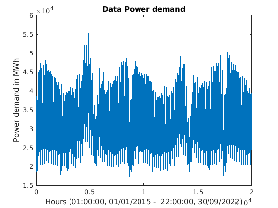
(a) Historical data of aggregate power demand in Italy (MWh).

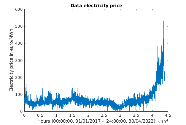
(b) Historical data of electricity spot price in Italy ( €/MWh).

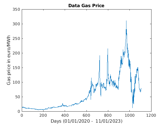
(c) Historical data of gas spot price in Italy (€/MWh).

Figure 2: Data set

To estimate the parameters of our four Brownian motions, we first removed seasonality from the three data series using harmonic regression [1]. In table 1 are presented the significant frequencies for the three data series, the corresponding periods and the approximate interpretation of these values.

Demand			Gas price			Electricity price
Frequency	Period	Meaning	Frequency	Period	Meaning	Frequency	Period	Meaning
0.04168	23.99232	1 day	0.00271	369.0037	1 year	0.08335	11.9976	half day
0.00595	168.0672	1 week	0.00542	184.5018	6 months	0.04165	24.0096	1 day
0.00035	2857.143	4 months	0.01085	92.1659	3 months	0.00595	168.0672	1 week
0.0007	1428.571	2 months	0.00814	122.8501	4 months	0.01190	84.03361	half week
0.08336	11.99616	Half day

Table 1: Significant frequencies

Then we estimate the parameters $\mu_{d}$, $\mu_{v}$, $\mu_{p}$ and $\sigma_{d}$, $\sigma_{v}$ and $\sigma_{p}$ using least squares estimator as in [2]. In Tables 4, 5, 6, 5 and are presented the result of our estimations considering different subset of the power demand and electricity price data set.

Parameter	value
$d$ (MW)	33197.38
$x_{v}$ (€/MWh)	56.7

Table 2: Intercepts for the electricity price and power demand series (not including 2020-2022)

Parameter	value
$d$ (MW)	32900.63
$x_{v}$ (€/MWh)	100

Table 3: Intercepts for the electricity price and power demand series (including 2020-2022)

Parameter	Estimated value
$\sigma_{d}$ $(1/\sqrt{h})$	0.03812835
$\sigma_{v}$ $(1/\sqrt{h})$	0.09281802

Table 4: Estimated volatility for the electricity price and power demand series (not including 2020-2022)

Parameter	Estimated value
$\sigma_{d}$ $(1/\sqrt{h})$	0.0366732
$\sigma_{v}$ $(1/\sqrt{h})$	0.0678185

Table 5: Estimated volatility for the electricity price and power demand series (including 2020-2022)

Even though the period 2020-2022 produced a unusual behavior in the evolution of the electricity spot price, we observe that the estimated volatility is lower than the one estimated using the data set not including the period 2020-2022. We can explain this apparent counterintuitive decrease on the value of the volatility arguing that we are observing the absolute prices and the GBM model consider the relative volatility.

Parameter	Estimated value	Confidence interval	Modified
$\mu_{d}$ (1/h)	$-8.470937\cdot 10^{-6}$	$(-0.0003654055,0.0003484636)$	$-7.268855\cdot 10^{-4}$
$\mu_{v}$ (1/h)	$-1.954675\cdot 10^{-5}$	$(-0.001141761,0.001102667)$	-0.004307592

Table 6: Estimated drift for the electricity price and power demand series (not including 2020-2022)

Parameter	Estimated value	Confidence interval	Modified
$\mu_{d}$ (1/h)	$4.923461\cdot 10^{-6}$	$(-0.0003152595,0.0003251064)$	$-6.724617\cdot 10^{-4}$
$\mu_{v}$ (1/h)	$1.042185\cdot 10^{-5}$	$(-0.0006247345,0.0006455782)$	$-0.002299817$

Table 7: Estimated drift for the electricity price and power demand series (including 2020-2022)

Since the data series of the gas spot price is from 2020 to 2023, corresponding to particular periods for the economy (COVID pandemic and Russia-Ukraine war), we estimate the parameters for the geometric Brownian motion considering the whole series and we do not distinguish between ”normal” periods as in the case of the series of power demand and electricity price, where we understand as ”normal” period the series not including the COVID pandemic period 2020-2022.

Parameter	Value
$p$ (€/MW)	74.7
$\sigma_{p}$ $(1/\sqrt{h})$	0.8371437
$\mu_{p}$ (1/h)	0.01539092
Confidence interval for $\mu_{p}$	$(-0.009429719,0.0107123)$
Martingale $\mu_{p}$	-0.3504048

Table 8: Estimated parameters for the gas series

A quite natural scenario used to set up a REC is where the members suppose that the ”world will proceed as it is” in that moment. For them to agree about if trends or volatilities will be definitely increasing or decreasing in the long run is of paramount difficulty. Indeed fixing the plant capacity and the sharing rules are decisions which tend to remain fixed through time for quite obvious reasons. So a world evolving in a martingale way is quite a neutral and natural setting which is interesting to adopt for our application. As our main purpose is to model an energy community and not to model prices or power demand we manipulate the values for the three drifts $\mu_{d}$, $\mu_{v}$ and $\mu_{p}$ in order to obtain martingale process, maintaining the values of the volatilities $\sigma_{d}$, $\sigma_{v}$ and $\sigma_{p}$.

4.2 Scenarios

4.2.1 Example 1

In table 9 are presented the real values used as application of our model.

Parameter	Value
$r$	$3.4247\cdot 10^{-6}$ 1/h
$c_{h}$	$2500000$ €/MW
$c_{b}$	$900000$ €/MW
$\theta_{h}$	$0.32$ MW
$\theta_{b}$	$0.2$ MW
$Z$	$110$ €/MWh
$K_{g}$	$18.9394$ $m^{3}$
$\rho_{c}$	0.01
$\lambda$	0.00001

Table 9: Constants

The constraint $\theta_{h}$ in Table 9 is related to the budget of the household, in this case we suppose a budget of $800000$ €, therefore $\theta_{h}=800000/c_{h}$. Instead we let $\theta_{b}=0.2$ MW, which is the maximum installation that the biogas can perform in order to receive the incentive $Z$.

Parameter	Value
$x_{v}$	$56.7$ €/MWh
$x_{c}$	$65$ €/MWh
$p$	$74.7$ €/MWh
$d$	$0.3$ MW

Table 10: Initial condition

In this case we use the parameters presented in tables 6, 4 and 8. We consider the modified drift in order to satisfy the integrability conditions in Assumption 3.1.

Parameter	Estimated Value
$\sigma_{v}$	0.09281802
$\sigma_{p}$	$0.8371437$
$\sigma_{d}$	0.03812835

Table 11: volatility for the spot electricity price, spot gas price and power demand

Parameter	Estimated Value
$\mu_{v}$	-0.004307592418360
$\mu_{p}$	$-0.350404787224845$
$\mu_{d}$	$-7.268855368612499\cdot 10^{-4}$

Table 12: Drift for the spot electricity price, spot gas price and power demand

Parameter	Estimated Value
$\sigma_{c}$	0.00128
$\mu_{c}$	$-2.1400\cdot^{-6}$

Table 13: Drift and volatility for the purchase electricity price

Parameter	value
$\beta_{b}$	-42.6169
$g_{h}$	$1.4056\cdot 10^{7}$
$g_{b}$	$-6.256\cdot 10^{-6}$

Table 14: Cases

From table 14 we observe that we are in the case $g_{h}>0$ and $g_{b}<0$. If we select, for example $\beta=0.2$, we have

$$g_{b}+Z\frac{(1-\beta)}{(r+\lambda)}=2.991\cdot 10^{5}>0,$$

therefore, the coordinator must to find a fair $\beta$ in order to incentive the investment of the biogas producer. Form 14 we observe that $\beta>\beta_{b}$ and therefore the Nash equilibrium is attained for

$$y_{h}^{*}=\theta_{h}$$

and

$$y_{b}^{*}=\max\left(\min\left(d\left(\frac{1-\beta}{1-\beta_{b}}\frac{g_{b}+Z\frac{1-\beta_{b}}{r+\lambda}}{g_{b}+Z\frac{1-\beta}{r+\lambda}}\right)^{1/m_{1}}-y_{h}^{*},\theta_{b}\right),0\right),$$

but even if we select the best $\beta$ for the biogas, i.e., $\beta=0$, its best response is equal to $y_{b}^{*}=0$, since

$$d\left(\frac{1-\beta}{1-\beta_{b}}\frac{g_{b}+Z\frac{1-\beta_{b}}{r+\lambda}}{g_{b}+Z\frac{1-\beta}{r+\lambda}}\right)^{1/m_{1}}-y_{h}^{*}=-0.0320.$$

Therefore, in this case the community is not performed.

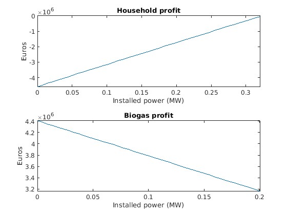
Figure 3: Household and biogas producer profits

We performed sensibility analysis over parameters $\sigma_{v}$, $\sigma_{d}$, $\sigma_{p}$, $\sigma_{c}$, $c_{b}$, $c_{h}$, $x_{v}$, $x_{c}$, $p$ and $d$. Here we present the most interesting cases.

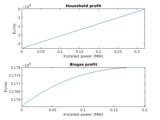
(a) Initial gas price $p=53.45$ €/MWh

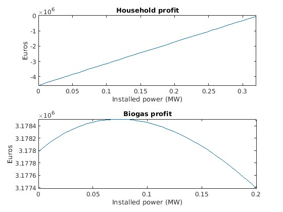
(b) Initial gas price $p=53.5$ €/MWh

Figure 4: Difference between installation strategies for different values of $p$

$p=53.45$ €/MWh		$p=53.5$ €/MWh
Parameter	Value	Parameter	Value
$y_{h}^{*}$	$\theta_{h}$	$y_{h}^{*}$	$\theta_{h}$
$y_{b}^{*}$	$0.1887$ MW	$y_{b}^{*}$	$0.0737$ MW
$\beta$	0.3913	$\beta$	0.3969

Table 15: Optimal installation strategies and fair division

4.2.2 Example 2

Similarly as in the Example 4.2.1, Tables 16, 17, 19, 19 and 20 present the real values used as application of our model.

Parameter	Value
$r$	$3.4247\cdot 10^{-6}$ 1/h
$c_{h}$	$1900000$ €/MW
$c_{b}$	$1100000$ €/MW
$\theta_{h}$	$0.4737$ MW
$\theta_{b}$	$0.2$ MW
$Z$	$110$ €/MWh
$K_{g}$	$18.9394$ $m^{3}$
$\rho_{c}$	0.01
$\lambda$	0.00001

Table 16: Constants

Parameter	Value
$x_{v}$	$80$ €/MWh
$x_{c}$	$85$ €/MWh
$p$	$68$ €/MWh
$d$	$0.3$ MW

Table 17: Initial condition

Parameter	Estimated Value
$\sigma_{v}$	0.0928
$\sigma_{p}$	$0.75$
$\sigma_{d}$	0.0019

Table 18: volatility for the spot electricity price, spot gas price and power demand

Parameter	Estimated Value
$\mu_{v}$	-0.0043
$\mu_{p}$	$-0.350$
$\mu_{d}$	$-7.269\cdot 10^{-4}$

Table 19: Drift for the spot electricity price, spot gas price and power demand

Parameter	Estimated Value
$\sigma_{c}$	0.0008
$\mu_{c}$	$-2.14\cdot^{-6}$

Table 20: Drift and volatility for the purchase electricity price

Parameter	value
$\beta_{b}$	$3.864\cdot 10^{4}$
$\beta_{h}$	$-3.652\cdot 10^{4}$
$g_{h}$	$1.3795\cdot 10^{7}$
$g_{b}$	$1.4594\cdot 10^{7}$

Table 21: Cases

From table 21 we observe that the best strategy for both memeber is to invest their maximum capacity, i.e. $y_{h}^{*}=\theta_{h}$ and $y_{b}^{*}=\theta_{b}$. In figure 5 are presented both profits.

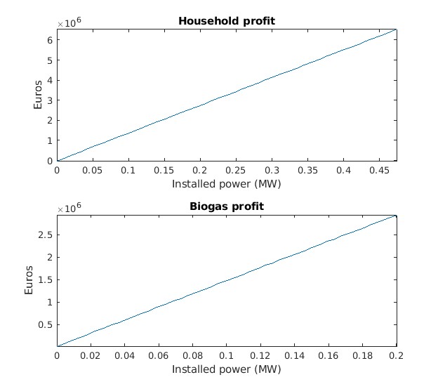
Figure 5: Household and biogas producer profits

As in the first example we performed a sensitivity analysis with respect to the variables $\sigma_{v}$, $\sigma_{d}$, $\sigma_{p}$, $\sigma_{c}$, $c_{b}$, $c_{h}$, $x_{v}$, $x_{c}$, $p$ and $d$. The most interested results are presented in this section. In Figure 6 we observe how the strategy of the potential members change as the electricity spot price decrease.

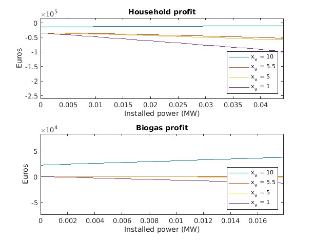
Figure 6: Sensitivity w.r.t. $x_{v}$

In Table 22 the corresponding optimal installation and the fair $\beta$ are presented for the the four cases highlighted in figure 6. We found that for some electricity spot price under 10 €/MWh the optimal strategy for both member is to install until a certain level. In this case we define the optimal strategy as thee corresponding Nash equilibrium of the game. In the three cases $x_{v}=1$, $x_{v}=5$, $x_{v}=5.5$ the interval $(\beta_{h},\beta^{b})$ is empty and therefore the parameter $\beta_{n}\notin(\beta_{h},\beta^{b})$ and the optimal aggregate installation does not exceed the power demand of the community.

$x_{v}=10$ €/MWh		$x_{v}=5.5$ €/MWh		$x_{v}=5$ €/MWh		$x_{v}=1$ €/MWh
Parameter	Value	Parameter	Value	Parameter	Value	Parameter	Value
$y_{h}^{*}$ (MW)	$\theta_{h}$	$y_{h}^{*}$ (MW)	$4.2117\cdot 10^{-4}$	$y_{h}^{*}$ (MW)	$9.7342\cdot 10^{-5}$	$y_{h}^{*}$ (MW)	$1.4605\cdot 10^{-10}$
$y_{b}^{*}$ (MW)	$\theta_{b}$	$y_{b}^{*}$ (MW)	$4.2117\cdot 10^{-4}$	$y_{b}^{*}$ (MW)	$9.7342\cdot 10^{-5}$	$y_{b}^{*}$ (MW)	$1.4605\cdot 10^{-10}$
$\beta$	0.5	$\beta$	0.974	$\beta$	0.8845	$\beta$	0.6532

Table 22: Optimal installation strategies and fair division

(a) Installation cost $c_{h}=15700000$ €/MWh

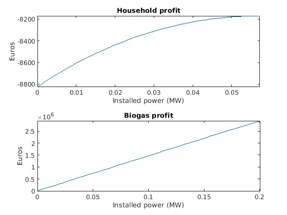
(b) Installation cost $c_{h}=157100000$ €/MWh

Figure 7: Difference between installation strategies for different values of $c_{h}$

$c_{h}=15700000$ €/MWh		$c_{h}=157100000$ €/MWh
Parameter	Value	Parameter	Value
$y_{h}^{*}$	$0.0573$	$y_{h}^{*}$	$0.05728$
$y_{b}^{*}$	$\theta_{b}$ MW	$y_{b}^{*}$	$\theta_{b}$ MW
$\beta$	0.5031	$\beta$	0.6244

Table 23: Optimal installation strategies and fair division

5 Conclusions

The topic of renewable energy communities (REC) is going to be of large relevance to the modern energy systems, since self-production and self-consumption at a local scale reduces the problem of grid congestion on the large scale. Despite RECs are expected to be groups composed by small numbers of members, the problems that they are required to face and solve are quite sophisticated. In this paper we consider a REC composed of two specific kind of members, namely an household and a biogas producer. Moreover, we consider an incentive scheme for self-consumption, which replicates the one adopted in Italy. As we has shown, the economic benefit accruing to the members of a REC depend on their joint decision about the size of their plants and the decision on the percentage to be applied to share the incentive on the energy self-consumed within the community. The two decisions interact, and finding a jointly optimal solution is of course of key importance to guarantee that the member agree to enter and remain within the community. By developing a leader-follower game, where the leader decide the division of the incentive and the followers decide the new power installation, we solve the problem.

As future research we can include the changes in photovoltaic energy production during the day and the night. To do so it is enough to consider a dynamic conversion factor $\alpha(s)$ such that $\alpha(s)y_{h}$ represent the photovoltaic energy. The energy produced using biogas is not as variable as the photovoltaic energy and our version of the model is accurate enough.

Another difficult and interesting extension of this model is to analyze the optimal irreversible investment problem, meaning that we are not anymore in a static framework but dynamic, where we can consider that the power demand follows some stochastic process.

Appendix A Appendix

Proof. (Lemma 3.4) First of all we notice that $w$ depends on $y_{b},y_{h}\geq 0$ only as parameters, as the nontrivial dependence is on $d$. For this reason, in this proof we will indicate explicitly only the dependence on $d$. Then if we assume that $\tau\sim Exp(\lambda)$ and is independent of $W_{d}$, then its randomness can be eliminated from the computation of $w$ in this way:

$$w(d) = \mathbb{E}\left[\int_{0}^{\tau}e^{-rs}\min\left\{D^{d}(s),y_{h}+y_{b}\right\}ds\right]=$$

$$= \mathbb{E}\left[\mathbb{E}\left[\left.\int_{0}^{\tau}e^{-rs}\min\left\{D^{d}(s),y_{h}+y_{b}\right\}ds\right|{\mathcal{F}}_{\tau}\right]\right]=$$

$$= \mathbb{E}\left[\int_{0}^{\tau}e^{-rs}\mathbb{E}\left[\left.\min\left\{D^{d}(s),y_{h}+y_{b}\right\}\right|{\mathcal{F}}_{\tau}\right]ds\right]=$$

$$= \mathbb{E}\left[\int_{0}^{\tau}e^{-rs}\mathbb{E}\left[\min\left\{D^{d}(s),y_{h}+y_{b}\right\}\right]ds\right]=$$

$$= \int_{0}^{\infty}\lambda e^{-\lambda u}\int_{0}^{u}e^{-rs}\mathbb{E}\left[\min\left\{D^{d}(s),y_{h}+y_{b}\right\}\right]ds\ du=$$

$$= \int_{0}^{\infty}e^{-rs}\mathbb{E}\left[\min\left\{D^{d}(s),y_{h}+y_{b}\right\}\right]\int_{s}^{\infty}\lambda e^{-\lambda u}du\ ds=$$

$$= \int_{0}^{\infty}e^{-(r+\lambda)s}\mathbb{E}\left[\min\left\{D^{d}(s),y_{h}+y_{b}\right\}\right]ds=$$

$$= \mathbb{E}\left[\int_{0}^{\infty}e^{-(r+\lambda)s}\min\left\{D^{d}(s),y_{h}+y_{b}\right\}ds\right]$$

where we use the independence between $\tau$ and $W_{d}$ (thus $D$) in the fourth equality and the Tonelli theorem in the sixth and in the eighth.

We can easily check that, with this new formulation, $w$ satisfies the ordinary differential equation (ODE)

$$(r+\lambda)w(d)-\mathcal{L}w(d)=\min(d,y_{h}+y_{b})$$ (23)

where $\mathcal{L}u(d)=\left(\mu_{d}+\frac{\sigma_{d}^{2}}{2}\right)du^{\prime}(d)+\frac{\sigma_{d}^{2}}{2}d^{2}u^{\prime\prime}(d)$. In fact, the general solution of Equation (23) is

$$w(d)=\begin{cases}Ad^{m_{1}}+Bd^{m_{2}}+\frac{d}{r_{d}+\lambda}&d<y_{h}+y_{b}\\ Cd^{m_{1}}+Dd^{m_{2}}+\frac{y_{h}+y_{b}}{r+\lambda}&d\geq y_{h}+y_{b}\end{cases}$$ (24)

where $A$, $B$, $C$ and $D$ are constants to be determined. As we want Equation (6) to hold, we want $w(0)=0$, therefore we must have $A=0$. On the other hand, when $d\rightarrow\infty$, we expect $w(d)\rightarrow\infty$, which gives $D=0$. Since Equation (23) is a linear second-order ODE with continuous coefficients, we expect its solution to be of class $C^{2}({\mathbb{R}}^{+})$. For this reason, we impose the value matching and smooth pasting conditions at at $d=y_{h}+y_{b}$, which imply

$$\begin{cases}B(y_{h}+y_{b})^{m_{2}}+\frac{y_{h}+y_{b}}{r_{d}+\lambda}=C(y_{h}+y_{b})^{m_{1}}+\frac{y_{h}+y_{b}}{r+\lambda}\\ Bm_{2}(y_{h}+y_{b})^{m_{2}-1}+\frac{1}{r_{d}+\lambda}=Cm_{1}(y_{h}+y_{b})^{m_{1}-1},\end{cases}$$ (25)

which gives

$$\begin{cases}B=(y_{h}+y_{b})^{1-m_{2}}B_{1}\\ C=(y_{h}+y_{b})^{1-m_{1}}C_{1},\end{cases}$$ (26)

with $B_{1}$ and $C_{1}$ as in Equation (9). With this determination, one can easily check that the function $w$ is increasing and concave on ${\mathcal{R}}^{+}$, and $C^{2}$ in $d$. We can easily check that $w$ is $C^{2}$ also in $y_{h}$ and $y_{b}$. In fact, it is outside of the region $\{y_{b}+y_{h}=d\}$. Moreover,

$$\left.w_{y_{b}}\right|_{y_{b}+y_{h}=d^{+}}=\left.w_{y_{h}}\right|_{y_{b}+y_{h}=d^{+}}=B_{1}(1-m_{2})=\left.w_{y_{b}}\right|_{y_{b}+y_{h}=d^{-}}=\left.w_{y_{h}}\right|_{y_{b}+y_{h}=d^{-}}=C_{1}(1-m_{1})+\frac{1}{r+\lambda}$$ (27)

which is easily obtained from the system (25) by simplifying for $(y_{b}+y_{h})$ in the first equation and subtracting the second. The fact that the second derivatives are also continuous at $\{y_{b}+y_{h}=d\}$ can be verified with some algebra.

By applying the Ito formula to the process $(e^{-(r+\lambda)t}w(D(t)))_{t}$ from $0$ to $T$, we have

$$e^{-(r+\lambda)T}w(D^{d}(T))=w(d)+\int_{0}^{T}e^{-(r+\lambda)s}\left(\mathcal{L}w(D^{d}(s))-(r+\lambda)w(D^{d}(s))\right)ds$$

$$+\int_{0}^{T}\sigma_{d}e^{-(r+\lambda)s}D^{d}(s)w^{\prime}(D^{d}(s))dW_{d}(s)$$

$$= w(d)-\int_{0}^{T}e^{-(r+\lambda)s}\min\{D^{d}(s),y_{h}+y_{b}\}ds+\int_{0}^{T}\sigma_{d}e^{-(r+\lambda)s}D^{d}(s)w^{\prime}(D^{d}(s))dW_{d}(s).$$

One can easily check that $w$ is concave, thus $|w^{\prime}(d)|\leq w^{\prime}(0)<+\infty$ for all $d\geq 0$: this implies

$$\mathbb{E}\left[\int_{0}^{T}e^{-2(r+\lambda)s}D^{2}(t)(w^{\prime}(D(t))^{2}dt\right] \leq \mathbb{E}\left[\int_{0}^{T}e^{-2(r+\lambda)s}D^{2}(t)(w^{\prime}(0))^{2}dt\right]$$

$$= \frac{1}{r_{d}^{2}}\int_{0}^{T}e^{-2s(r+\lambda-\mu_{d})}\mathbb{E}\left[e^{2\sigma_{d}W(s)}\right]ds$$

$$= \frac{1}{r_{d}^{2}}\int_{0}^{T}e^{-2s(r+\lambda-\mu_{d}-\sigma_{d}^{2})}ds<\infty$$

thus the expectation of the stochastic integral above is zero and we have that, for all $T>0$,

$$w(d)=\mathbb{E}\left[e^{-(r+\lambda)T}w(D^{d}(T))\right]+\mathbb{E}\left[\int_{0}^{T}e^{-(r+\lambda)s}\min\{D^{d}(s),y_{h}+y_{b}\}ds\right]$$ (28)

Finally, since for all $d\geq 0$ we have

$$0\leq w(d)\leq\lim_{d\to+\infty}w(d)=\frac{y_{h}+y_{b}}{r+\lambda},$$

then

$$\lim_{T\rightarrow\infty}\left|\mathbb{E}\left[e^{-(r+\lambda)T}w(D^{d}(T))\right]\right|\leq\lim_{T\rightarrow\infty}e^{-(r+\lambda)T}\frac{y_{h}+y_{b}}{r+\lambda}=0,$$

and by letting $T\to+\infty$ in Equation (28), we get the result in Equation (6).   

Proof. (Proposition 3.5) We can find the point of maximum of $J_{h}$ using a first order condition. The partial derivative of $J_{h}$ w.r.t. $y_{h}$ is given by

$$\frac{\partial J_{h}}{\partial y_{h}}=\begin{cases}g_{h}+Z\beta B_{1}d^{m_{2}}(1-m_{2})(y_{h}+y_{b})^{-m_{2}}&d<y_{h}+y_{b}\\ g_{h}+Z\beta(C_{1}d^{m_{1}}(1-m_{1})(y_{h}+y_{b})^{-m_{1}}+\frac{1}{r+\lambda})&d\geq y_{h}+y_{b}.\end{cases}$$ (29)

$\frac{\partial J_{h}}{\partial y_{h}}$ is continuous in $y_{h}$, then we search for the critical point $\frac{\partial J_{h}}{\partial y_{h}}=0$. As $y_{h}\in[0,\theta_{h}]$ we also have to consider the extreme points $0$ and $\theta_{h}$.

Since $J_{h}$ is $C^{1}$ and concave in $y_{h}$ , we can determine whether the maximum is attained when the aggregate installation is greater than the demand or not, by observing the sign of $\frac{\partial J_{h}}{\partial y_{h}}|_{y_{h}=d-y_{b}}$. In fact $\frac{\partial J_{h}}{\partial y_{h}}|_{y_{h}=d-y_{b}}\lesseqgtr 0$ if and only if the maximum $y_{h}^{*}\lesseqgtr d-y_{b}$.

We have that

$$\left.\frac{\partial J_{h}}{\partial y_{h}}\right|_{y_{h}=d-y_{b}}=g_{h}+Z\beta B_{1}(1-m_{2})$$

thus, since $B_{1}<0$ and $m_{2}>1$, we have that $\frac{\partial J_{h}}{\partial y_{h}}|_{y_{h}=d-y_{b}}>0$ if and only if $\beta>\beta_{h}$, this latter being defined in Equation (12).

Let us move into the solution of problem (10). Let us suppose $\beta>\beta_{h}$, so that $\frac{\partial J_{h}}{\partial y_{h}}|_{y_{h}=d-y_{b}}>0$: then we know that the maximum is attained when the installation exceeds the demand, i.e. when $d<y_{b}+y_{h}$. The first-order condition (29) are solved, in the case $d<y_{h}+y_{b}$, for

$$Z\beta B_{1}d^{m_{2}}(m_{2}-1)(y_{h}+y_{b})^{-m_{2}}=g_{h}$$

As the left-hand side is always negative, the first-order condition has a solution only if $g_{h}<0$. In this case, $\beta>\beta_{h}>0$ and the solution is

$$y_{h}^{*}=d\left(\frac{Z\beta B_{1}(m_{2}-1)}{g_{h}}\right)^{1/m_{2}}-y_{b}{=d\left(\frac{\beta}{\beta_{h}}\right)^{1/m_{2}}-y_{b}}.$$

If $y_{h}^{*}\in[0,\theta_{h}]$, then $y_{h}^{*}$ is the maximum. If $y_{h}^{*}<0$ then the maximum is 0 and if $y_{h}^{*}>\theta_{h}$ then the maximum . is $\theta_{h}$. Moreover, if $ZB_{1}(m_{2}-1)<g_{h}$, then $\beta_{h}<1$ . Summarizing,

$$y_{h}^{*}=\max\left\{\min\left\{d\left(\frac{\beta}{\beta_{h}}\right)^{1/m_{2}}-y_{b},\theta_{h}\right\},0\right\}.$$ (30)

Instead, if $g_{h}\geq 0$, then the first-order condition is not satisfied, $\frac{\partial J_{h}}{\partial y_{h}}$ is always positive and the maximum of $J_{h}$ is reached for $y_{h}^{*}=\theta_{h}$. In this case $\beta_{h}<0$.

Let us now suppose that $\beta\leq\beta_{h}$, i.e. $\frac{\partial J_{h}}{\partial y_{h}}|_{y_{h}=d-y_{b}}\leq 0$. Then for $d\geq y_{h}+y_{b}$, the first order condition is solved for

$$Z\beta C_{1}d^{m_{1}}(m_{1}-1)(y_{h}+y_{b})^{-m_{1}}=g_{h}+\frac{Z\beta}{r+\lambda},$$

as the left hand side is always positive, the first order condition has a solution only if $g_{h}+\frac{Z\beta}{r+\lambda}>0$, and the solution is

$$y_{h}^{*}=d\left(\frac{Z\beta C_{1}(m_{1}-1)}{g_{h}+\frac{Z\beta}{r+\lambda}}\right)^{1/m_{1}}-y_{b}{=d\left(\frac{\frac{g_{h}}{\beta_{h}}+\frac{Z}{r+\lambda}}{\frac{g_{h}}{\beta}+\frac{Z}{r+\lambda}}\right)^{1/m_{1}}-y_{b}}.$$

moreover if $g_{h}<0$, then $\beta_{h}>0$. If $y_{h}^{*}\in[0,\theta_{h}]$, then $y_{h}^{*}$ is the maximum. If $y_{h}^{*}<0$ then the maximum will be attained at zero, and if $y_{h}^{*}>\theta_{h}$ then the maximum will be attained at $\theta_{h}$. Summarizing,

$$y_{h}^{*}=\max\left\{\min\left\{d\left(\frac{\frac{g_{h}}{\beta_{h}}+\frac{Z}{r+\lambda}}{\frac{g_{h}}{\beta}+\frac{Z}{r+\lambda}}\right)^{1/m_{1}}-y_{b},\theta_{h}\right\},0\right\}.$$ (31)

On the other hand, if $g_{h}+\frac{Z\beta}{r+\lambda}\leq 0$, the derivative is always negative and the maximum is always attained at $y_{h}^{*}=0$. Again in this case $\beta_{h}>0$.

 

Proof. (Proposition 3.7) We can find the point of maximum of $J_{b}$ using a first order condition. The partial derivative of $J_{b}$ w.r.t. $y_{b}$ is given by

$$\frac{\partial J_{b}}{\partial y_{b}}=\begin{cases}g_{b}+Z(1-\beta)\left(B_{1}(1-m_{2})(y_{h}+y_{b})^{-m_{2}}d^{m_{2}}\right)&d<y_{h}+y_{b}\\ g_{b}+Z(1-\beta)\left(C_{1}(1-m_{1})(y_{h}+y_{b})^{-m_{1}}d^{m_{1}}+\frac{1}{r+\lambda}\right)&d\geq y_{h}+y_{b}.\end{cases}$$ (32)

$\frac{\partial J_{b}}{\partial y_{b}}$ is continuous in $y_{b}$, then we search for the critical point $\frac{\partial J_{b}}{\partial y_{b}}=0$. As $y_{b}\in[0,\theta_{b}]$ we also have to consider the extreme points $0$ and $\theta_{b}$.

Since $J_{b}$ is $C^{1}$ in $y_{b}$ and it is concave, we can determine whether the maximum is attained when the aggregate installation surplus the demand or not, by observing the sign of $\frac{\partial J_{b}}{\partial y_{b}}|_{y_{b}=d-y_{h}}$. In fact $\frac{\partial J_{b}}{\partial y_{b}}|_{y_{b}=d-y_{h}}\lesseqgtr 0$ if and only if the maximum $y_{b}^{*}\lesseqgtr d-y_{h}$.

We have that

$$\left.\frac{\partial J_{b}}{\partial y_{b}}\right|_{y_{b}=d-y_{h}}=g_{b}+Z(1-\beta)B_{1}(1-m_{2})=g_{b}+Z(1-\beta)\left(C_{1}(1-m_{1})+\frac{1}{r+\lambda}\right)$$

thus, since $B_{1}<0$ and $m_{2}>1$, we have that $\frac{\partial J_{b}}{\partial y_{b}}|_{y_{b}=d-y_{h}}>0$ if and only if $1-\beta>1-\beta_{b}$ with $\beta_{b}$ defined in Equation (15).

Let us move into the solution of problem (13). Let us suppose $\beta<\beta_{b}$, i.e. $\frac{\partial J_{b}}{\partial y_{b}}|_{y_{b}=d-y_{h}}>0$, then we know that the maximum is attained when the installation exceeds the demand, i.e. $d<y_{h}+y_{b}$: the first-order condition is then solved for

$$g_{b}=Z(1-\beta)\left(B_{1}(m_{2}-1)(y_{h}+y_{b})^{-m_{2}}d^{m_{2}}\right).$$

Since the right-hand side is always negative, the first order condition has a solution only if $g_{b}<0$ and the solution is

$$y_{b}^{*}=d\left(\frac{Z(1-\beta)B_{1}(m_{2}-1)}{g_{b}}\right)^{1/m_{2}}-y_{h}{=d\left(\frac{1-\beta}{1-\beta_{b}}\right)^{1/m_{2}}-y_{h}}.$$

If $y_{b}^{*}\in[0,\theta_{b}]$, then it is the maximum. If $y_{b}^{*}>\theta_{b}$, then we select $\theta_{b}$ as optimal point, instead if $y_{b}^{*}<0$, we select $y_{b}^{*}=0$. Moreover, if $g_{b}>ZB_{1}(m_{2}-1)$, then $\beta^{b}>0$. Summarizing,

$$y_{b}^{*}=\max\left\{\min\left\{d\left(\frac{1-\beta}{1-\beta_{b}}\right)^{1/m_{2}}-y_{h},\theta_{b}\right\},0\right\}.$$ (33)

In the case $g_{b}\geq 0$, the derivative is always positive and the maximum is attained at $y_{b}^{*}=\theta_{b}$.

In analogy with the previous case, let us now suppose $\beta\geq\beta_{b}$, i.e. $\frac{\partial J_{b}}{\partial y_{b}}|_{y_{b}=d-y_{h}}\leq 0$, in this case $d\geq y_{h}+y_{b}$. The first order condition is now solved for

$$g_{b}+\frac{Z(1-\beta)}{r+\lambda}=Z(1-\beta)\left(C_{1}(m_{1}-1)(y_{h}+y_{b})^{-m_{1}}d^{m_{1}}\right).$$

Since the right-hand side is always positive, the first order condition is solved only if $g_{b}+\frac{Z(1-\beta)}{r+\lambda}>0$ and the solution is

$$y_{b}^{*}=d\left(\frac{Z(1-\beta)C_{1}(m_{1}-1)}{g_{b}+\frac{Z(1-\beta)}{r+\lambda}}\right)^{1/m_{1}}-y_{h}=d\left(\frac{\frac{g_{b}}{1-\beta_{b}}+\frac{Z}{r+\lambda}}{\frac{g_{b}}{1-\beta}+\frac{Z}{r+\lambda}}\right)^{1/m_{1}}-y_{h}$$ (34)

If $y_{b}^{*}\in[0,\theta_{b}]$, then it is the maximum. If $y_{b}^{*}>\theta_{b}$, then we select $\theta_{b}$ as optimal point, instead if $y_{b}^{*}<0$, we select $y_{b}^{*}=0$. If, moreover, $g_{b}<0$, then $\beta^{b}<1$. Furthermore, if it is verified that $ZB_{1}(m_{2}-1)<g_{b}$, then $\beta^{b}>0$. Summarizing,

$$y_{b}^{*}=\max\left\{\min\left\{d\left(\frac{\frac{g_{b}}{1-\beta_{b}}+\frac{Z}{r+\lambda}}{\frac{g_{b}}{1-\beta}+\frac{Z}{r+\lambda}}\right)^{1/m_{1}}-y_{h},\theta_{b}\right\},0\right\}.$$ (35)

In the case $g_{b}+\frac{Z(1-\beta)}{r+\lambda}\leq 0$, the derivative is always negative and the maximum is attained at $y_{b}^{*}=0$.   

Proof. (Proposition 3.9) We start by proving that the strategies presented in (16), (17) and (18) are Nash equilibria. In all these cases the community is performed if the biogas investment is positive. We will prove only the most interesting or representative cases, the other cases can be proved analogously.

Let us start with the case $g_{h}+\frac{Z\beta}{r+\lambda}>0>g_{h}$, $g_{b}+\frac{Z(1-\beta)}{r+\lambda}>0>g_{b}$ and $\beta=\beta_{n}$. Suppose $\beta_{n}\in(\beta_{h},\beta^{b})$ (The same arguments can be applied for $\beta_{n}\notin(\beta_{h},\beta^{b})$). In this case we will check if any strategy of the form

$$y_{h}^{*} = \alpha\max\left\{\min\left\{d\left(\frac{ZB_{1}(m_{2}-1)}{g_{h}+g_{b}}\right)^{1/m_{2}},\theta_{h}\right\},0\right\},$$

$$y_{b}^{*} = (1-\alpha)\max\left\{\min\left\{d\left(\frac{ZB_{1}(m_{2}-1)}{g_{h}+g_{b}}\right)^{1/m_{2}},\theta_{b}\right\},0\right\},$$

with $\alpha\in(0,1)$ is a Nash equilibrium.

For the household profit we have

$$J_{h}(x_{v},x_{c},p,d,y_{h},y_{b}^{*},\beta) = y_{h}g_{h}-\frac{x_{c}d}{r_{cd}}+\beta_{n}Zw(y_{h},y_{b}^{*},d)\noindent$$ (36)

$$= y_{h}g_{h}-\frac{x_{c}d}{r_{cd}}+\left(\frac{g_{h}}{g_{h}+g_{b}}\right)Z\left(B_{1}(y_{h}+y_{b}^{*})^{1-m_{2}}+\frac{d}{r_{d}+\lambda}\right),$$ (37)

as $J_{h}$ is concave in $y_{h}$, we can find its maximum by applying first order conditions. By direct computation we find that

$$\operatorname*{arg\,max}_{y_{h}\in[0,\theta_{h}]}J_{h}(x_{v},x_{c},p,d,y_{h},y_{b}^{*}) = \alpha\max\left\{\min\left\{d\left(\frac{ZB_{1}(m_{2}-1)}{g_{h}+g_{b}}\right)^{1/m_{2}},\theta_{h}\right\},0\right\}.$$ (38)

On the other hand, for the biogas profit we have,

$$J_{b}(x_{v},x_{c},p,d,y_{h}^{*},y_{b}) = y_{b}g_{b}+\frac{pbK_{g}}{r_{p}}+(1-\beta_{n})Zw(y_{h}^{*},y_{b},d)$$

$$= y_{b}g_{b}+\frac{pbK_{g}}{r_{p}}+(1-\frac{g_{h}}{g_{h}+g_{b}})Z\left(B_{1}(y_{h}^{*}+y_{b})^{1-m_{2}}+\frac{d}{r_{d}+\lambda}\right).$$

Analogously to the household profit, $J_{b}$ in concave in $y_{b}$ and we can find its maximum by applying first order conditions. By direct computation we find that

$$\operatorname*{arg\,max}_{y_{b}\in[0,\theta_{b}]}J_{b}(x_{v},x_{c},p,d,y_{h}^{*},y_{b}) = (1-\alpha)\max\left\{\min\left\{d\left(\frac{ZB_{1}(m_{2}-1)}{g_{h}+g_{b}}\right)^{1/m_{2}},\theta_{h}\right\},0\right\}.$$ (39)

By (38) and (39) the strategies (36) satisfy definition (7) and therefore any linear combination $\alpha\in(0,1)$ is a Nash equilibria.

The value of $\beta_{n}$ comes from the computation of the best responses of the household and biogas producer. From propositions 3.6 and 3.8 we know that in the case $\beta<\beta^{b}$ and $\beta>\beta_{h}$ (the same is valid in the case $\beta\geq\beta^{b}$ and $\beta\leq\beta_{h}$) the best responses are

$$y_{h}^{*} = \max\left\{\min\left\{\displaystyle d\left(\frac{\beta}{\beta_{h}}\right)^{1/m_{2}}-y_{b},\theta_{h}\right\},0\right\},$$ (40)

$$y_{b}^{*} = \max\left\{\min\left\{d\left(\frac{1-\beta}{1-\beta_{b}}\right)^{1/m_{2}}-y_{h},\theta_{b}\right\},0\right\}.$$ (41)

Suppose

$$y_{h}^{*} = \displaystyle d\left(\frac{\beta}{\beta_{h}}\right)^{1/m_{2}}-y_{b},$$ (42)

$$y_{b}^{*} = d\left(\frac{1-\beta}{1-\beta_{b}}\right)^{1/m_{2}}-y_{h}.$$ (43)

The system (42) has solutions only if

$$y_{h}^{*}+y_{b}^{*}=\left(\frac{\beta}{\beta_{h}}\right)^{1/m_{2}}=d\left(\frac{1-\beta}{1-\beta_{b}}\right)^{1/m_{2}},$$

which implies

$$\beta=\frac{\beta_{h}}{1-\beta^{b}+\beta_{h}}:=\beta_{n}.$$

In all the other possible cases in (40), the system is solvable for any $\beta\in(0,1)$ and the value for the optimum $\beta$ is computed by solving the coordinators problem (3.5.1).

Case $g_{h}>0$, $g_{b}>0$. For the household profit we have

$$J_{h}(x_{v},x_{c},p,d,y_{h},\theta_{b},\beta)=y_{h}g_{h}-\frac{x_{c}d}{r_{cd}}+\beta Zw(y_{h},\theta_{b},d).$$

The function $J_{h}$ has positive derivative, therefore its maximum is attained at $y_{h}^{*}=\theta_{h}$. The same is valid for the for the biogas profit,

$$J_{b}(x_{v},x_{c},p,d,\theta_{h},y_{b},\beta)=y_{b}g_{b}+\frac{pbK_{g}}{r_{p}}+(1-\beta)Zw(\theta_{h},y_{b},d),$$

which is also increasing in $y_{b}$ and therefore its maximum is attained at $\theta_{b}$. We conclude $(\theta_{h},\theta_{b})$ is a Nash equilibrium.

Case $g_{h}+\frac{Z\beta}{r+\lambda}\leq 0$ and $g_{b}\geq 0$. By (29) we know that the function $J_{h}$ is decreasing in $y_{h}$ and therefore its maximum is attained at $0$. By (32) the function $J_{b}$ is increasing in $y_{b}$ , therefore its maximum is attained at $\theta_{b}$, which demonstrate (7).

Case $g_{h}<0\leq g_{h}+\frac{Z\beta}{r+\lambda}$, $\beta>\beta_{h}$ (the case $\beta\leq\beta_{h}$ can be proved analogously) and $g_{b}\geq 0$. By the same arguments of the previous case, $J_{b}$ is increasing in $y_{b}$ and therefore it maximum is attained at $y_{b}^{*}=\theta_{b}$. On the other hand, the household profit become

$$J_{h}(x_{v},x_{c},p,d,y_{h},\theta_{b},\beta)=y_{h}g_{h}-\frac{x_{c}d}{r_{cd}}+\beta Z\left(B_{1}(y_{h}+\theta_{b})^{1-m_{2}}+\frac{d}{r_{d}+\lambda}\right).$$

By applying first order condition we find that

$$\operatorname*{arg\,max}_{y_{h}\in[0,\theta_{h}]}J_{h}(x_{v},x_{c},p,d,y_{h},\theta_{h},\beta) = \max\left\{\min\left\{d\left(\frac{\beta}{\beta_{h}}\right)^{1/m_{2}}-\theta_{b},\theta_{h}\right\},0\right\},$$ (44)

which prove definition (7).

References

• [1] Bloomfield, P. (2007). Fourier Analysis of Time Series: An Introduction. Wiley series in probability and mathematical statistics.
• [2] Brigo, D., Dalessandro, A., Neugebauer, M., Triki, F. (2008). A Stochastic Processes Toolkit for Risk Management. Available at https://arxiv.org/abs/0812.4210.
• [3] European Parliament. Directive (EU) 2018/2001 of the European Parliament and of the Council of 11 December 2018 on the promotion of the use of energy from renewable sources. Available at https://eur-lex.europa.eu/eli/dir/2018/2001/oj
• [4] European Parliament. Directive (EU) 2019/944 of the European Parliament and of the Council of 5 June 2019 on common rules for the internal market for electricity and amending Directive 2012/27/EU. Available at https://eur-lex.europa.eu/eli/dir/2019/944/oj
• [5] Italian Government. Law decree 162/2019. Urgent provisions on the extension of legislative terms, organization of the public administrations and technological innovation. https://www.gazzettaufficiale.it/eli/id/2019/12/31/19G00171/sg
• [6] Italian Ministry of Ecological Transition (MITE). Decree 2020, September 16. On the identification of the incentive tariff for the remuneration of renewable energy plants. https://www.gazzettaufficiale.it/eli/id/2020/11/16/20A06224/sg
• [7] Italian Parliament. Law 8/2020, Conversion to Law of the Law decree 162/2019, with amendments. https://www.gazzettaufficiale.it/eli/id/2020/02/29/20G00021/sg
• [8] Moncecchi, M., Meneghello, S., Merlo, M. (2020). A Game Theoretic Approach for Energy Sharing in the Italian Renewable Energy Communities. Applied Sciences, 10(22), 8166.
• [9] Peters, H. (2008). Game Theory: A multilevel approach. Springer Berlin, Heidelberg.
• [10] Pham, H. (2009). Continuous-time Stochastic Control and Optimization with Financial Applications. Springer, Berlin, Heidelberg.
• [11] Pirjol, D., Zhu, L. (2016). Discrete sums of geometric Brownian motions, annuities and Asian options. Insurance: Mathematics and Economics, 70 19-37.
• [12] U.S. Energy Information Administration. International Energy Outlook 2021. Available online at https://www.eia.gov/outlooks/ieo/pdf/IEO2021_ChartLibrary_full.pdf
• [13] Löbbe, S., Sioshansi, F., Robinson, D. (2022). Energy Communities: Customer-Centered, Market-Driven, Welfare-Enhancing? Elsevier Science.
• [14] Tushar, W., Yuen, C., Mohsenian-Rad, H., Saha, T., Poor, H. V., Wood, K. L. (2018). Transforming Energy Networks via Peer-to-Peer Energy Trading: The Potential of Game-Theoretic Approaches. IEEE Signal Processing Magazine, 35(4) 90-111.
• [15] Manuel De Villena, M., Aittahar, S., Mathieu, S., Boukas, I., Vermeulen, E., Ernst, D. (2022). Financial Optimization of Renewable Energy Communities Through Optimal Allocation of Locally Generated Electricity. IEEE Access 10 77571-77586.
• [16] Safdarian, A., Astero, P., Baranauskas, M., Keski-Koukkari, A., Kulmala, A. (2021). Coalitional Game Theory Based Value Sharing in Energy Communities. IEEE Access 9 78266-78275.
• [17] Mitridati, L., Kazempour, J., Pinson, P. (2021). Design and game-Theoretic analysis of community-Based market mechanisms in heat and electricity systems. Omega, 99 102 - 177.
• [18] Abada, I., Ehrenmann, A., Lambin, X. (2017). On the viability of energy communities. Energy Policy Research Group, University of Cambridge.
• [19] Anoh, K., Maharjan, S., Ikpehai, A., Zhang, Y., Adebisi, B. (2020). Energy Peer-to-Peer Trading in Virtual Microgrids in Smart Grids: A Game-Theoretic Approach. IEEE Transactions on Smart Grid, 11(2) 1264-1275.
• [20] Paudel, A., Chaudhari, K., Long, C., Gooi, H. B. (2019). Peer-to-Peer Energy Trading in a Prosumer-Based Community Microgrid: A Game-Theoretic Model. IEEE Transactions on Industrial Electronics 66(8) 6087-6097.
• [21] Candelise, C., Ruggieri, G. (2020). Status and Evolution of the Community Energy Sector in Italy. Energies, 13 (8) 1888.
• [22] Tushar, W., Saha, T. K., Yuen, C., Morstyn, T., McCulloch, M.D., Poor, H.V., Wood, K.L. (2019). A motivational game-theoretic approach for peer-to-peer energy trading in the smart grid. Applied Energy, 243 10-20.
• [23] Feng, C., Wen, F., You, S., Li, Z., Shahnia, F., Shahidehpour, M. (2020). Coalitional Game-Based Transactive Energy Management in Local Energy Communities. IEEE Transactions on Power Systems, 35(3) 1729-1740.
• [24] Gjorgievski, V.Z., Cundeva, S., Georghiou, G.E. (2021). Social arrangements, technical designs and impacts of energy communities: A review. Renewable Energy, 169 1138-1156.
• [25] Norbu, S., Couraud, B., Robu, V., Andoni, M., Flynn, D. (2021). Modelling the redistribution of benefits from joint investments in community energy projects. Applied Energy, 287 116575.
• [26] Li, L. (2020). Optimal Coordination Strategies for Load Service Entity and Community Energy Systems Based on Centralized and Decentralized Approaches. Energies, 13 (12) 3202.
• [27] Zatti, M., Moncecchi, M., Gabba, M., Chiesa, A., Bovera, F., Merlo, M. (2021). Energy Communities Design Optimization in the Italian Framework. Applied Sciences, 11(11) 5218.
• [28] Cutore, E., Volpe, R., Sgroi, R., Fichera, A. (2023). Energy management and sustainability assessment of renewable energy communities: The Italian context. Energy Conversion and Management, 278 116713.
• [29] Dimovski, A., Moncecchi, M., Merlo, M. (2023). Impact of energy communities on the distribution network: An Italian case study. Sustainable Energy, Grids and Networks, 35 101148.
• [30] De Juan-Vela, P., Alic, A., Trovato, V. (2023). Monitoring the Italian transposition of the EU regulation concerning renewable energy communities and the relevant policies for battery storage. Journal of Cleaner Production, 425 138937.
• [31] Musolino, M., Maggio, G., D’Aleo, E., Nicita, A. (2023). Three case studies to explore relevant features of emerging renewable energy communities in Italy. Renewable Energy, 210 540-555.
• [32] Lilliu, F., Denysiuk, R., Reforgiato Recupero, D., Vinyals, M. (2021). A Game-Theoretical Incentive Mechanism for Local Energy Communities. Agents and Artificial Intelligence, Springer International Publishing, 52-72.
• [33] Toderean, L., Chifu, V. R., Cioara, T., Anghel, I., Pop, C. B. (2023). Cooperative Games Over Blockchain and Smart Contracts for Self-Sufficient Energy Communities. IEEE Access, 11 73982-73999.
• [34] https://www.eia.gov/energyexplained/units-and-calculators/energy-conversion-calculators.php