Convergence of the PML method for the biharmonic wave scattering problem in periodic structures

Abstract

This paper investigates the scattering of biharmonic waves by a one-dimensional periodic array of cavities embedded in an infinite elastic thin plate. The transparent boundary conditions are introduced to formulate the problem from an unbounded domain to a bounded one. The well-posedness of the associated variational problem is demonstrated utilizing the Fredholm alternative theorem. The perfectly matched layer (PML) method is employed to reformulate the original scattering problem, transforming it from an unbounded domain to a bounded one. The transparent boundary conditions for the PML problem are deduced, and the well-posedness of its variational problem is established. Moreover, exponential convergence is achieved between the solution of the PML problem and that of the original scattering problem.

2010]78A45, 65N30

1 Introduction

Scattering of flexural waves in an elastic thin plate, modeled by fourth-order biharmonic wave equations, holds broad engineering applications. These applications span diverse fields, including the design of ultra-broadband elastic cloaking [1, 2, 3], platonic crystals [4, 5, 6], and the exploration of acoustic black hole concepts [7]. Consequently, ongoing research in theoretical analysis, numerical simulations, and industrial manufacturing continues to draw considerable attention from both engineering and mathematical communities.

Most works in the literature focus on the static problem in a bounded domain, which is formulated by the bi-Laplacian equation. When addressing the fourth-order problem using the finite element method, standard $H^{2}$-conforming methods necessitate $C^{1}$-continuous piecewise polynomials on the mesh, a challenge in practical implementation. Alternatively, various nonconforming and discontinuous finite element methods have emerged, such as the weak Galerkin finite element methods supplemented with stabilizers [8, 9, 10]; the virtual element method, which requires no global $C^{0}$ regularity for the numerical solution [11, 12]; and the mixed element method, effectively reducing the fourth-order problem to coupled second-order problems [13, 14, 15, 16]. These methods have undergone comprehensive analysis.

When compared with the results concerning the bi-Laplacian equation, the findings are relatively limited for the biharmonic wave scattering problems in unbounded domains. In [17], the initial theoretical analysis of the boundary integral equation method was provided for solving the biharmonic wave equation. Through the introduction of two auxiliary variables, the biharmonic wave equation was split into the Helmholtz and modified Helmholtz equations. Subsequently, the Holmholtz and modified Helmholtz wave components were represented using the double- and single-layer potentials. The well-posedness of the coupled boundary integral system was established by applying the Riesz–Fredholm theory. If the exterior problem is approached using the variational approach with transparent boundary conditions (TBCs), the studies concerning waveguide and obstacle scattering problems were presented in [18, 19] under various boundary conditions, including clamped, simply supported, roller-supported, or free plate boundary conditions. Numerically, a mixed element method was proposed in [20, 21] by introducing two auxiliary variables and decomposing the biharmonic problem into the Helmholtz and modified Helmholtz equations. Subsequently, TBCs were introduced for each equation. Particularly, the linear finite element method, incorporating interior penalty and boundary penalty, was proposed in [21] to effectively reduce the oscillation of the bending moment.

The method of perfectly matched layer (PML) is a widely utilized domain truncation technique. In contrast to the nonlocal TBC method, the PML method generates a local boundary condition on the outer surface of the layer by integrating an artificial absorbing region around the domain of interest. The ease of handling the local boundary condition has contributed to the widespread adoption of this method ever since its inception by Bérenger [22] for solving the time-dependent Maxwell equations. It has found extensive applications in solving various wave scattering problems, including, for example, acoustic waves [23], electromagnetic waves [24, 25, 26], and elastic waves [27, 28]. The PML method has also been utilized numerically in solving biharmonic wave scattering problems [29, 30, 31], highlighting its convenience and accuracy. However, to our knowledge, a comprehensive discussion regarding the well-posedness of the PML method and its convergence has not been documented in existing literature. This paper aims to address these gaps.

In this paper, we investigate the scattering of flexural waves resulting from a plane incident wave interacting with a one-dimensional periodic array of cavities within an infinite elastic thin plate. The wave propagation is described by the fourth-order biharmonic wave equation. Because of the periodic characteristics of both the incident wave and the cavities, the solution complies with quasi-periodic conditions, allowing us to formulate the problem within a single periodic cell. The TBCs are derived by incorporating the bounded outgoing wave condition, utilizing the Fourier series expansion of the solution in regions distant from the cavities. With the aid of the TBCs, the scattering problem is equivalently transformed from an unbounded domain to a bounded one. The corresponding variational problem is shown to satisfy Gårding’s inequality, and its well-posedness is established through the utilization of the Fredholm alternative theorem. To replace the nonlocal TBCs, the PML method is adopted through the complex coordinate stretching scheme [32]. Alternatively, the unbounded domain is truncated by imposing homogeneous boundary conditions on the wave field and its normal derivative at the outer boundary of the PML region. Upon studying the Fourier series expansion of the solution to the PML problem, we deduce equivalent TBCs to reformulate the PML problem in the domain where the original scattering problem, along with the TBC, is imposed. The well-posedness of the PML problem is confirmed through an examination of its variational formulation. Additionally, the PML solution demonstrates exponential convergence concerning the thickness of the PML regions towards the solution of the original scattering problem. For a comprehensive account of related electromagnetic wave scattering problems in periodic structures, we reference [33].

The paper is outlined as follows. Section 2 introduces the model equations. The TBCs are derived in Section 3. Section 4 details the reduction of the scattering problem to a bounded domain using the TBCs, along with the discussion on the well-posedness of the variational problem. Section 5 addresses the PML problem, including investigations into its well-posedness and convergence. Finally, the paper concludes with general remarks in Section 6.

2 Problem formulation

Let us examine the scattering phenomenon of an incident wave interacting with a one-dimensional periodic array of cavities in an infinitely extending elastic thin plate, which is characterized by the Kirchhoff–Love model and is depicted in Figure 1. Assume that the alignment of the cavities coincides with the $x_{1}$-axis, exhibiting a periodicity of $\Lambda$. Consider an incident field represented as a time-harmonic plane wave given by

$$u^{i}(x)=e^{{\rm i}(\alpha x_{1}-\beta x_{2})},\quad x\in\mathbb{R}^{2},$$

where $\alpha=\kappa\sin\theta,\beta=\kappa\cos\theta$ with $\kappa>0$ and $\theta\in\left(-\frac{\pi}{2},\frac{\pi}{2}\right)$ denoting the wavenumber and the incident angle, respectively. It can be verified that the incident field $u^{i}$ satisfies the biharmonic wave equation

$$\Delta^{2}u^{i}-\kappa^{4}u^{i}=0\quad\text{in}~{}\mathbb{R}^{2}.$$

Due to the periodic nature of the geometry, the problem can be confined to a single periodic cell. Denote by $\Omega_{c}$ the cavity with a Lipschitz continuous boundary $\Gamma_{c}$. Let $R$ be a rectangular domain that is sufficiently large to enclose the region $\Omega_{c}$. Without loss of generality, let $R$ be defined as $R=\left\{x\in\mathbb{R}^{2}:0<x_{1}<\Lambda,h_{2}<x_{2}<h_{1}\right\}$, where $h_{k},k=1,2$ are constants. Additionally, define $\Gamma_{k}=\left\{x\in\mathbb{R}^{2}:0<x_{1}<\Lambda,x_{2}=h_{k}\right\}$ for $k=1,2$, $\Gamma_{l}=\left\{x\in\mathbb{R}^{2}:x_{1}=0,h_{2}<x_{2}<h_{1}\right\}$, and $\Gamma_{r}=\left\{x\in\mathbb{R}^{2}:x_{1}=\Lambda,h_{2}<x_{2}<h_{1}\right\}$. Let $\Omega=R\setminus\overline{\Omega_{c}}$. Define $\Omega_{1}$ and $\Omega_{2}$ as the regions above and below $\Gamma_{1}$ and $\Gamma_{2}$, respectively.

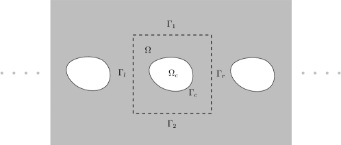
Figure 1: Schematic of the problem geometry.

The out-of-plane displacement of the plate, denoted as $u$ and referred to as the total field, also satisfies the biharmonic wave equation

$$\Delta^{2}u-\kappa^{4}u=0\quad{\rm in}~{}\Omega.$$ (1)

The total field is assumed to satisfy the Dirichlet boundary condition, known as the clamped boundary condition, on $\Gamma_{c}$:

$$u=0,\quad\partial_{\nu}u=0,$$ (2)

where $\nu$ denotes the unit normal vector on $\Gamma_{c}$. It is worth noting that other types of boundary conditions, such as the Neumann boundary condition, often known as the free plate boundary condition, can be similarly taken into account.

Given the periodic nature of both the structure and the incident wave, the solution to (1)–(2) demonstrates quasi-periodicity. Specifically, if $u$ is a solution to (1)–(2), then $u(x)e^{-{\rm i}\alpha x_{1}}$ is a periodic function of $x_{1}$ with a period of $\Lambda$. This characteristic gives rise to the quasi-periodic boundary condition on $\Gamma_{l}$ and $\Gamma_{r}$, i.e., $u$ satisfies $u(0,x_{2})=e^{-{\rm i}\alpha\Lambda}u(\Lambda,x_{2})$. Furthermore, to ensure the well-posedness of the problem, it is essential to impose a bounded outgoing wave condition on the scattered field $u^{s}=u-u^{i}$ in $\Omega_{1}$ and the total field $u$ in $\Omega_{2}$.

We introduce notations and function spaces employed in this work. Denote by $H^{2}(\Omega)$ the standard Sobolev space, comprising functions with square-integrable values, as well as square-integrable first and second partial derivatives. Let us define the quasi-periodic function space

$$H_{\rm qp}^{2}(\Omega)=\left\{u\in H^{2}(\Omega):u(\Lambda,x_{2})=u(0,x_{2})e^{{\rm i}\alpha\Lambda}\right\},$$

along with its subspace

$$H_{{\rm qp},\Gamma_{c}}^{2}(\Omega)=\left\{u\in H^{2}_{\rm qp}(\Omega):u=0,\partial_{\nu}u=0\text{ on }\Gamma_{c}\right\}.$$

Clearly, $H_{\rm qp}^{2}(\Omega)$ and $H_{{\rm qp},\Gamma_{c}}^{2}(\Omega)$ are subspaces of $H^{2}(\Omega)$ equipped with the standard $H^{2}$-norm.

Given a function $u\in H_{\rm qp}^{2}(\Omega)$, it allows for a Fourier expansion on $\Gamma_{k},k=1,2:$

$$u(x,h_{k})=\sum\limits_{n\in\mathbb{Z}}u^{(n)}(h_{k})e^{{\rm i}\alpha_{n}x_{1}},$$

where

$$\alpha_{n}=\alpha+n\left(\frac{2\pi}{\Lambda}\right),\quad u^{(n)}(h_{k})=\frac{1}{\Lambda}\int_{0}^{\Lambda}u(x,h_{k})e^{-{\rm i}\alpha_{n}x_{1}}{\rm d}x_{1}.$$

The trace function space $H^{s}(\Gamma_{k})$, where $s\in\mathbb{R}$, is defined as follows:

$$H^{s}(\Gamma_{k})=\left\{u\in L^{2}(\Gamma_{k}):\|u\|_{H^{s}(\Gamma_{k})}<\infty\right\},$$

with the norm given by

$$\|u\|_{H^{s}(\Gamma_{k})}=\left(\Lambda\sum\limits_{n\in\mathbb{Z}}\left(1+\alpha_{n}^{2}\right)^{s}|u^{(n)}(h_{k})|^{2}\right)^{1/2}.$$

In this paper, whenever $a\lesssim b$ is used, it denotes $a\leq Cb$, with $C$ representing a positive constant. In this context, the values of the constants $c_{j}$ are positive and may vary in different steps of the proof. Although the specific values of $C$ and $c_{j}$ are not explicitly stated, their dependence should be apparent from the context.

3 Transparent boundary conditions

In this section, we address the challenge posed by formulating the problem in an unbounded domain. To overcome this obstacle, we propose introducing an equivalent transparent boundary condition (TBC) on $\Gamma_{k},k=1,2$ with the objective of transforming the problem into the bounded domain $\Omega$.

Let $\nu=(\nu_{1},\nu_{2})$ and $\tau=(\tau_{1},\tau_{2})$ be the unit normal and tangent vectors, respectively, to the boundary of $\Omega$. Clearly, we have $\tau_{1}=-\nu_{2}$ and $\tau_{2}=\nu_{1}$. Define the normal and tangential derivatives

$$\partial_{\nu}:=\nu_{1}\partial_{x_{1}}+\nu_{2}\partial_{x_{2}},\quad\partial_{\tau}:=-\nu_{2}\partial_{x_{1}}+\nu_{1}\partial_{x_{2}}.$$

For $0\leq\mu<1$, referred to as the Poisson ratio, define the surface differential operators (cf. [34]):

$$Mu:=\mu\Delta u+(1-\mu)M_{0}u,\quad Nu:=-\partial_{\nu}\Delta u-(1-\mu)\partial_{\tau}N_{0}u,$$ (3)

where $M_{0}$ and $N_{0}$ are explicitly given by

$$\left\{\begin{aligned} &M_{0}u:=\nu_{1}^{2}\frac{\partial^{2}u}{\partial x_{1}^{2}}+2\nu_{1}\nu_{2}\frac{\partial^{2}u}{\partial x_{1}\partial x_{2}}+\nu_{2}^{2}\frac{\partial^{2}u}{\partial x_{2}^{2}},\\ &N_{0}u:=\left(\nu_{1}^{2}-\nu_{2}^{2}\right)\frac{\partial^{2}u}{\partial x_{1}\partial x_{2}}-\nu_{1}\nu_{2}\left(\frac{\partial^{2}u}{\partial x_{1}^{2}}-\frac{\partial^{2}u}{\partial x_{2}^{2}}\right).\end{aligned}\right.$$

First, we derive the TBC on $\Gamma_{1}$. Based on the bounded outgoing wave condition, it is shown in [20] that the scattered field $u^{s}$ can be represented by a Fourier series expansion in the domain $\Omega_{1}$:

$$u^{s}(x_{1},x_{2})=\sum\limits_{n\in\mathbb{Z}}H_{1}^{(n)}e^{{\rm i}\alpha_{n}x_{1}+{\rm i}\beta_{n}(x_{2}-h_{1})}+\sum\limits_{n\in\mathbb{Z}}U_{1}^{(n)}e^{{\rm i}\alpha_{n}x_{1}-\gamma_{n}(x_{2}-h_{1})},$$ (4)

where $H_{1}^{(n)},U_{1}^{(n)}\in\mathbb{C}$ are the Fourier coefficients, and

$$\beta_{n}=\left\{\begin{aligned} &(\kappa^{2}-\alpha_{n}^{2})^{1/2}\quad&&\text{if}~{}\kappa>|\alpha_{n}|,\\ &{\rm i}(\alpha_{n}^{2}-\kappa^{2})^{1/2}\quad&&\text{if}~{}\kappa<|\alpha_{n}|,\end{aligned}\right.\quad\gamma_{n}=(\kappa^{2}+\alpha_{n}^{2})^{1/2}.$$ (5)

Here, we assume that $\beta_{n}\neq 0$ for all $n\in\mathbb{Z}$ to rule out the occurrence of resonances.

Let $\left(u,\partial_{\nu}u\right)=(f_{1},g_{1})$ and $\left(u^{s},\partial_{\nu}u^{s}\right)=(\hat{f}_{1},\hat{g}_{1})$ be the Dirichlet data for the total and scattered fields on $\Gamma_{1}$, respectively. It is clear to note that these data satisfy the relations

$$f_{1}(x_{1})=\hat{f}_{1}(x_{1})+e^{{\rm i}\left(\alpha x_{1}-\beta h_{1}\right)},\quad g_{1}(x_{1})=\hat{g}_{1}(x_{1})-{\rm i}\beta e^{{\rm i}\left(\alpha x_{1}-\beta h_{1}\right)}.$$

Being quasi-periodic functions, $\hat{f}_{1}$ and $\hat{g}_{1}$ admit the Fourier series expansions

$$u^{s}(x_{1},h)=\hat{f}_{1}(x_{1})=\sum_{n\in\mathbb{Z}}\hat{f}_{1}^{(n)}e^{{\rm i}\alpha_{n}x_{1}},\quad\partial_{\nu}u^{s}(x_{1},h_{1})=\hat{g}_{1}(x_{1})=\sum_{n\in\mathbb{Z}}\hat{g}_{1}^{(n)}e^{{\rm i}\alpha_{n}x_{1}},$$

where $\hat{f}_{1}^{(n)},\hat{g}_{1}^{(n)}\in\mathbb{C}$ are the Fourier coefficients.

On the other hand, evaluating the scattered field $u^{s}$, as defined in (4), and its normal derivative $\partial_{x_{2}}u^{s}$ on $\Gamma_{1}$, we obtain

$$\left\{\begin{aligned} u^{s}(x_{1},h_{1})&=\sum\limits_{n\in\mathbb{Z}}H_{1}^{(n)}e^{{\rm i}\alpha_{n}x_{1}}+\sum\limits_{n\in\mathbb{Z}}U_{1}^{(n)}e^{{\rm i}\alpha_{n}x_{1}},\\ \partial_{x_{2}}u^{s}(x_{1},h_{1})&=\sum\limits_{n\in\mathbb{Z}}{\rm i}\beta_{n}H_{1}^{(n)}e^{{\rm i}\alpha_{n}x_{1}}-\sum\limits_{n\in\mathbb{Z}}\gamma_{n}U_{1}^{(n)}e^{{\rm i}\alpha_{n}x_{1}}.\end{aligned}\right.$$

Combining the above equations, we have from straightforward calculations that the scattered field $u^{s}$ in domain $\Omega_{1}$ can be expressed as

$$u^{s}(x_{1},x_{2}) =\sum\limits_{n\in\mathbb{Z}}\left(\frac{\gamma_{n}\hat{f}^{(n)}_{1}+\hat{g}^{(n)}_{1}}{\gamma_{n}+{\rm i}\beta_{n}}\right)e^{{\rm i}\alpha_{n}x_{1}+{\rm i}\beta_{n}(x_{2}-h_{1})}$$

$$\quad+\sum\limits_{n\in\mathbb{Z}}\left(\frac{{\rm i}\beta_{n}\hat{f}^{(n)}_{1}-\hat{g}^{(n)}_{1}}{\gamma_{n}+{\rm i}\beta_{n}}\right)e^{{\rm i}\alpha_{n}x_{1}-\gamma_{n}(x_{2}-h_{1})}.$$ (6)

On $\Gamma_{1}$, the surface differential operators $M$ and $N$ given in (3) can be simplified to

$$N_{1}u=-(2-\mu)\frac{\partial^{3}u}{\partial x_{1}^{2}\partial x_{2}}-\frac{\partial^{3}u}{\partial x_{2}^{3}},\quad M_{1}u=\mu\frac{\partial^{2}u}{\partial x_{1}^{2}}+\frac{\partial^{2}u}{\partial x_{2}^{2}}.$$ (7)

Substituting (3) into (7) yields the TBC of the scattered field $u^{s}$ on $\Gamma_{1}$:

$$N_{1}u^{s}=T_{11}^{(1)}\hat{f}_{1}+T_{12}^{(1)}\hat{g}_{1},\quad M_{1}u^{s}=T_{21}^{(1)}\hat{f}_{1}+T_{22}^{(1)}\hat{g}_{1}.$$

Here, the Dirichlet-to-Neumann (DtN) operators $T_{ij}^{(1)},i,j=1,2$ are given by

$$\left\{\begin{aligned} (T_{11}^{(1)}f)(x_{1})&=\sum\limits_{n\in\mathbb{Z}}{\rm i}\beta_{n}\gamma_{n}\left(\gamma_{n}-{\rm i}\beta_{n}\right)f^{(n)}e^{{\rm i}\alpha_{n}x_{1}},\\ (T_{21}^{(1)}f)(x_{1})&=-\sum\limits_{n\in\mathbb{Z}}\left(\mu\alpha_{n}^{2}-{\rm i}\beta_{n}\gamma_{n}\right)f^{(n)}e^{{\rm i}\alpha_{n}x_{1}},\\ (T_{12}^{(1)}g)(x_{1})&=-\sum\limits_{n\in\mathbb{Z}}\left(\mu\alpha_{n}^{2}-{\rm i}\beta_{n}\gamma_{n}\right)g^{(n)}e^{{\rm i}\alpha_{n}x_{1}},\\ (T_{22}^{(1)}g)(x_{1})&=-\sum\limits_{n\in\mathbb{Z}}\left(\gamma_{n}-{\rm i}\beta_{n}\right)g^{(n)}e^{{\rm i}\alpha_{n}x_{1}},\end{aligned}\right.$$ (8)

where $f^{(n)}$ and $g^{(n)}$ are the Fourier coefficients of $f$ and $g$, respectively. Noting $u=u^{s}+u^{i}$, we deduce the TBC for the total field $u$ on $\Gamma_{1}$:

$$N_{1}u=T_{11}^{(1)}f_{1}+T_{12}^{(1)}g_{1}+p_{1},\quad M_{1}u=T_{21}^{(1)}f_{1}+T_{22}^{(1)}g_{1}+p_{2}.$$ (9)

where

$$p_{1}(x_{1})=-\left(2{\rm i}\beta\alpha^{2}+2\beta^{2}\gamma\right)e^{{\rm i}(\alpha x_{1}-\beta h_{1})},\quad p_{2}(x_{1})=-(2\beta^{2}+2{\rm i}\beta\gamma)e^{{\rm i}(\alpha x_{1}-\beta h_{1})}.$$ (10)

Given the similarity in the derivation process of the TBC to that of $\Gamma_{2}$, we provide a brief overview of the procedure and present the resulting TBC. In accordance with the bounded outgoing wave condition, the total field $u$ exhibits the Fourier series expansion in $\Omega_{2}$:

$$u(x_{1},x_{2})=\sum\limits_{n\in\mathbb{Z}}H_{2}^{(n)}e^{{\rm i}\alpha_{n}x_{1}-{\rm i}\beta_{n}(x_{2}-h_{2})}+\sum\limits_{n\in\mathbb{Z}}U_{2}^{(n)}e^{{\rm i}\alpha_{n}x_{1}+\gamma_{n}(x_{2}-h_{2})}.$$ (11)

Evaluating (11) and its normal derivative on $\Gamma_{2}$, we obtain

$$\left\{\begin{aligned} u(x_{1},h_{2})&=\sum\limits_{n\in\mathbb{Z}}H_{2}^{(n)}e^{{\rm i}\alpha_{n}x_{1}}+\sum\limits_{n\in\mathbb{Z}}U_{2}^{(n)}e^{{\rm i}\alpha_{n}x_{1}}=\sum\limits_{n\in\mathbb{Z}}f^{(n)}_{2}e^{{\rm i}\alpha_{n}x_{1}},\\ \partial_{\nu}u(x_{1},h_{2})&=\sum\limits_{n\in\mathbb{Z}}{\rm i}\beta_{n}H_{2}^{(n)}e^{{\rm i}\alpha_{n}x_{1}}-\sum\limits_{n\in\mathbb{Z}}\gamma_{n}U_{2}^{(n)}e^{{\rm i}\alpha_{n}x_{1}}=\sum\limits_{n\in\mathbb{Z}}g^{(n)}_{2}e^{{\rm i}\alpha_{n}x_{1}},\end{aligned}\right.$$ (12)

where $(u,\partial_{\nu}u)=(f_{2},g_{2})$ are the Dirichlet data on $\Gamma_{2}$ and have the Fourier series expansions

$$f_{2}(x_{1})=\sum\limits_{n\in\mathbb{Z}}f^{(n)}_{2}e^{{\rm i}\alpha_{n}x_{1}},\quad g_{2}(x_{1})=\sum\limits_{n\in\mathbb{Z}}g^{(n)}_{2}e^{{\rm i}\alpha_{n}x_{1}}.$$

By solving the system (12), we deduce that the total field $u$ in $\Omega_{2}$ admits the Fourier series expansion

$$u(x_{1},x_{2}) =\sum\limits_{n\in\mathbb{Z}}\left(\frac{\gamma_{n}f^{(n)}_{2}+g^{(n)}_{2}}{\gamma_{n}+{\rm i}\beta_{n}}\right)e^{{\rm i}\alpha_{n}x_{1}-{\rm i}\beta_{n}(x_{2}-h_{2})}$$

$$\quad+\sum\limits_{n\in\mathbb{Z}}\left(\frac{{\rm i}\beta_{n}f^{(n)}_{2}-g^{(n)}_{2}}{\gamma_{n}+{\rm i}\beta_{n}}\right)e^{{\rm i}\alpha_{n}x_{1}+\gamma_{n}(x_{2}-h_{2})}.$$ (13)

Noting that the surface differential operator $M$ and $N$ on $\Gamma_{2}$ can be simplified to

$$N_{2}u=(2-\mu)\frac{\partial^{3}u}{\partial x_{1}^{2}\partial x_{2}}+\frac{\partial^{3}u}{\partial x_{2}^{3}},\quad M_{2}u=\mu\frac{\partial^{2}u}{\partial x_{1}^{2}}+\frac{\partial^{2}u}{\partial x_{2}^{2}},$$ (14)

we substitute (3) into (14) and obtain the TBC of the total field $u$ on $\Gamma_{2}$:

$$N_{2}u=T_{11}^{(2)}f_{2}+T_{12}^{(2)}g_{2},\quad M_{2}u=T_{21}^{(2)}f_{2}+T_{22}^{(2)}g_{2},$$ (15)

where the DTN operators $T_{ij}^{(2)},i,j=1,2$ are defined as

$$\left\{\begin{aligned} (T_{11}^{(2)}f)(x_{1})&=\sum\limits_{n\in\mathbb{Z}}{\rm i}\beta_{n}\gamma_{n}\left(\gamma_{n}-{\rm i}\beta_{n}\right)f^{(n)}_{2}e^{{\rm i}\alpha_{n}x_{1}},\\ (T_{21}^{(2)}f)(x_{1})&=-\sum\limits_{n\in\mathbb{Z}}\left(\mu\alpha_{n}^{2}-{\rm i}\beta_{n}\gamma_{n}\right)f^{(n)}_{2}e^{{\rm i}\alpha_{n}x_{1}},\\ (T_{12}^{(2)}g)(x_{1})&=-\sum\limits_{n\in\mathbb{Z}}\left(\mu\alpha_{n}^{2}-{\rm i}\beta_{n}\gamma_{n}\right)g^{(n)}_{2}e^{{\rm i}\alpha_{n}x_{1}},\\ (T_{22}^{(2)}g)(x_{1})&=-\sum\limits_{n\in\mathbb{Z}}\left(\gamma_{n}-{\rm i}\beta_{n}\right)g^{(n)}_{2}e^{{\rm i}\alpha_{n}x_{1}}.\end{aligned}\right.$$

The following result concerns the properties of the DtN operators $T^{(1)}_{ij}$ and $T^{(2)}_{ij}$, where $i,j=1,2.$

Lemma 1.

For $k=1,2$, the DtN operators $T^{(k)}_{11}:H^{3/2}(\Gamma_{k})\to H^{-3/2}(\Gamma_{k})$, $T^{(k)}_{12}:H^{1/2}(\Gamma_{k})\to H^{-3/2}(\Gamma_{k})$, $T^{(k)}_{21}:H^{3/2}(\Gamma_{k})\to H^{-1/2}(\Gamma_{k})$, and $T^{(k)}_{22}:H^{1/2}(\Gamma_{k})\to H^{-1/2}(\Gamma_{k})$ are bounded.

Proof.

We only prove the results for the operators $T_{ij}^{(1)}$, as the corresponding properties for the operators $T_{ij}^{(2)}$ can be obtained in the same manner. It is clear to note from (5) that

$$\lim\limits_{|n|\rightarrow\infty}\frac{|\beta_{n}|}{|\alpha_{n}|}=1,\quad\lim\limits_{|n|\rightarrow\infty}\frac{|\gamma_{n}|}{|\alpha_{n}|}=1.$$ (16)

For a given $f\in H^{3/2}(\Gamma_{1})$, we have from (8) and (16) that

$$\|T^{(1)}_{11}f\|^{2}_{H^{-3/2}(\Gamma_{1})} =\Lambda\sum\limits_{n\in\mathbb{Z}}\left(1+\alpha_{n}^{2}\right)^{-3/2}\big{|}{\rm i}\beta_{n}\gamma_{n}\left(\gamma_{n}-{\rm i}\beta_{n}\right)f^{(n)}\big{|}^{2}$$

$$\lesssim\sum\limits_{n\in\mathbb{Z}}(1+\alpha_{n}^{2})^{3/2}|f^{(n)}|^{2}\lesssim\|f\|^{2}_{H^{3/2}(\Gamma_{1})},$$

and

$$\|T^{(1)}_{21}f\|^{2}_{H^{-1/2}(\Gamma_{1})} =\Lambda\sum\limits_{n\in\mathbb{Z}}\left(1+\alpha_{n}^{2}\right)^{-1/2}\big{|}\left(\mu\alpha_{n}^{2}-{\rm i}\beta_{n}\gamma_{n}\right)f^{(n)}\big{|}^{2}$$

$$\lesssim\sum\limits_{n\in\mathbb{Z}}(1+\alpha_{n}^{2})^{3/2}|f^{(n)}|^{2}\lesssim\|f\|^{2}_{H^{3/2}(\Gamma_{1})}.$$

Similarly, for any function $f\in H^{1/2}(\Gamma_{1})$, we deduce from (8) and (16) that

$$\|T^{(1)}_{12}f\|^{2}_{H^{-3/2}(\Gamma_{1})} =\Lambda\sum\limits_{n\in\mathbb{Z}}\left(1+\alpha_{n}^{2}\right)^{-3/2}\big{|}\left(\mu\alpha_{n}^{2}-{\rm i}\beta_{n}\gamma_{n}\right)g^{(n)}\big{|}^{2}$$

$$\lesssim\sum\limits_{n\in\mathbb{Z}}(1+\alpha_{n}^{2})^{1/2}|f^{(n)}|^{2}\lesssim\|f\|^{2}_{H^{1/2}(\Gamma_{1})},$$

and

$$\|T^{(1)}_{22}f\|^{2}_{H^{-1/2}(\Gamma_{1})} =\Lambda\sum\limits_{n\in\mathbb{Z}}\left(1+\alpha_{n}^{2}\right)^{-1/2}\big{|}\left(\gamma_{n}-{\rm i}\beta_{n}\right)f^{(n)}\big{|}^{2}$$

$$\lesssim\sum\limits_{n\in\mathbb{Z}}(1+\alpha_{n}^{2})^{1/2}|f^{(n)}|^{2}\lesssim\|f\|^{2}_{H^{1/2}(\Gamma_{1})},$$

thus completing the proof. ∎

Lemma 2.

If $|n|$ is sufficiently large, then the following inequality holds for any complex values $f$ and $g$:

$$\Re\big{\{}-{\rm i}\beta_{n}\gamma_{n}\left(\gamma_{n}-{\rm i}\beta_{n}\right)|f|^{2}+\left(\mu\alpha_{n}^{2}-{\rm i}\beta_{n}\gamma_{n}\right)g\bar{f}$$

$$+\left(\mu\alpha_{n}^{2}-{\rm i}\beta_{n}\gamma_{n}\right)f\bar{g}+\left(\gamma_{n}-{\rm i}\beta_{n}\right)|g|^{2}\big{\}}\geq 0.$$

Proof.

By the definitions of $\gamma_{n}$ and $\beta_{n}$ given in (5), a straightforward calculation shows that for sufficiently large $|n|$

$$-{\rm i}\beta_{n}\gamma_{n}\left(\gamma_{n}-{\rm i}\beta_{n}\right)>0,\quad\mu\alpha_{n}^{2}-{\rm i}\beta_{n}\gamma_{n}>0,\quad\gamma_{n}-{\rm i}\beta_{n}>0.$$

It suffices to demonstrate for sufficiently large $|n|$ that

$$-{\rm i}\beta_{n}\gamma_{n}\left(\gamma_{n}-{\rm i}\beta_{n}\right)|f|^{2}-2\left(\mu\alpha_{n}^{2}-{\rm i}\beta_{n}\gamma_{n}\right)|f||g|+\left(\gamma_{n}-{\rm i}\beta_{n}\right)|g|^{2}\geq 0.$$

Utilizing the Cauchy inequality, we deduce from a simple calculation that

$$\big{(}(-{\rm i}\beta_{n}\gamma_{n})^{1/2}\left(\gamma_{n}-{\rm i}\beta_{n}\right)\big{)}^{2}-\big{(}\mu\alpha_{n}^{2}-{\rm i}\beta_{n}\gamma_{n}\big{)}^{2}$$

$$=-\gamma_{n}^{2}\beta_{n}^{2}-\mu\alpha_{n}^{4}-2{\rm i}(1-\mu)\gamma_{n}\beta_{n}\alpha_{n}^{2}$$

$$=\alpha_{n}^{4}-\kappa^{4}-\mu\alpha_{n}^{4}-2{\rm i}(1-\mu)\gamma_{n}\beta_{n}\alpha_{n}^{2}$$

$$=(1-\mu)\left(\alpha_{n}^{4}-2{\rm i}\gamma_{n}\beta_{n}\alpha_{n}^{2}\right)-\kappa^{4},$$

which is positive for sufficiently large $|n|$ by noting that $\mu<1$ and $\alpha_{n}^{4}-2{\rm i}\gamma_{n}\beta_{n}\alpha_{n}^{2}\to\infty$ as $|n|\to\infty$. ∎

Lemma 3.

For any $f\in H^{3/2}(\Gamma_{k})$ and $g\in H^{1/2}(\Gamma_{k})$ with $k=1,2$, there exists a positive constant $C$ such that

$$-\Re\left\{\int_{\Gamma_{k}}\Big{(}T_{11}^{(k)}|f|^{2}+T_{12}^{(k)}g\bar{f}+T_{21}^{(k)}f\bar{g}+T_{22}^{(k)}|g|^{2}\Big{)}{\rm d}s\right\}$$

$$\geq-C\Big{(}\|f\|^{2}_{L^{2}(\Gamma_{k})}+\|g\|^{2}_{L^{2}(\Gamma_{k})}\Big{)}.$$

Proof.

We prove the result for $k=1$, as the result for $k=2$ can be obtained similarly. By the definitions of $T^{(1)}_{ij}$ and Lemma 2, we have

$$-\Re\int_{\Gamma_{1}}\left(T_{11}^{(1)}|f|^{2}+T_{12}^{(1)}g\bar{f}+T_{21}^{(1)}f\bar{g}+T_{22}^{(1)}|g|^{2}\right){\rm d}s$$

$$=\Lambda\sum\limits_{|n|\leq n_{0}}\Re\Big{\{}-{\rm i}\beta_{n}\gamma_{n}\left(\gamma_{n}-{\rm i}\beta_{n}\right)|f^{(n)}|^{2}+\left(\mu\alpha_{n}^{2}-{\rm i}\beta_{n}\gamma_{n}\right)g^{(n)}\overline{f^{(n)}}$$

$$\quad+\left(\mu\alpha_{n}^{2}-{\rm i}\beta_{n}\gamma_{n}\right)f^{(n)}\overline{g^{(n)}}+\left(\gamma_{n}-{\rm i}\beta_{n}\right)|g^{(n)}|^{2}\Big{\}}$$

$$\quad+\Lambda\sum\limits_{|n|>n_{0}}\Re\Big{\{}-{\rm i}\beta_{n}\gamma_{n}\left(\gamma_{n}-{\rm i}\beta_{n}\right)|f^{(n)}|^{2}$$

$$\quad+\left(\mu\alpha_{n}^{2}-{\rm i}\beta_{n}\gamma_{n}\right)g^{(n)}\overline{f^{(n)}}+\left(\mu\alpha_{n}^{2}-{\rm i}\beta_{n}\gamma_{n}\right)f^{(n)}\overline{g^{(n)}}+\left(\gamma_{n}-{\rm i}\beta_{n}\right)|g^{(n)}|^{2}\Big{\}}$$

$$\geq\Lambda\sum\limits_{|n|\leq n_{0}}\Re\Big{\{}-{\rm i}\beta_{n}\gamma_{n}\left(\gamma_{n}-{\rm i}\beta_{n}\right)|f^{(n)}|^{2}+\left(\mu\alpha_{n}^{2}-{\rm i}\beta_{n}\gamma_{n}\right)g^{(n)}\overline{f^{(n)}}$$

$$\quad+\left(\mu\alpha_{n}^{2}-{\rm i}\beta_{n}\gamma_{n}\right)f^{(n)}\overline{g^{(n)}}+\left(\gamma_{n}-{\rm i}\beta_{n}\right)|g^{(n)}|^{2}\Big{\}}$$

$$\geq-C\left(\|f\|^{2}_{L^{2}(\Gamma_{1})}+\|g\|^{2}_{L^{2}(\Gamma_{1})}\right),$$

where $n_{0}$ is the smallest integer such that Lemma 2 holds. ∎

Utilizing the TBCs given by (9) and (15), we transform the original problem (1)–(2) from an unbounded domain into the bounded domain $\Omega$, which is to find a quasi-periodic function $u$ satisfying

$$\left\{\begin{aligned} &\Delta^{2}u-\kappa^{4}u=0&&\text{in}~{}\Omega,\\ &u=0,\quad\partial_{\nu}u=0&&\text{on}~{}\Gamma_{c},\\ &N_{1}u=T_{11}^{(1)}f_{1}+T_{12}^{(1)}g_{1}+p_{1}&&\text{on}~{}\Gamma_{1},\\ &M_{1}u=T_{21}^{(1)}f_{1}+T_{22}^{(1)}g_{1}+p_{2}&&\text{on}~{}\Gamma_{1},\\ &N_{2}u=T_{11}^{(2)}f_{2}+T_{12}^{(2)}g_{2}&&\text{on}~{}\Gamma_{2},\\ &M_{2}u=T_{21}^{(2)}f_{2}+T_{22}^{(2)}g_{2}&&\text{on}~{}\Gamma_{2},\end{aligned}\right.$$ (17)

where $p_{1}$ and $p_{2}$ are defined in (10), and $(f_{k},g_{k})$ are the Dirichlet data of the total field $u$ on $\Gamma_{k}$ for $k=1,2.$ The objective of this study is to examine the PML formulation applied to the boundary value problem (17) and to establish the convergence of the PML solution.

4 The variational problem

In this section, we present a variational formulation for the boundary value problem (17) and examine its well-posedness.

Observing that the bi-Laplacian can be expressed in terms of the Poisson ratio, as demonstrated in [34], we have

$$\Delta^{2}u-\kappa^{4}u =\frac{\partial^{2}}{\partial x_{1}^{2}}\left(\frac{\partial^{2}u}{\partial x_{1}^{2}}+\mu\frac{\partial^{2}u}{\partial x_{2}^{2}}\right)+2(1-\mu)\frac{\partial^{2}}{\partial x_{1}\partial x_{2}}\left(\frac{\partial^{2}u}{\partial x_{1}\partial x_{2}}\right)$$

$$\quad+\frac{\partial^{2}}{\partial x_{2}^{2}}\left(\frac{\partial^{2}u}{\partial x_{2}^{2}}+\mu\frac{\partial^{2}u}{\partial x_{1}^{2}}\right)-\kappa^{4}u.$$

Multipling both sides of the above equation with a test function $v\in H_{{\rm qp},\Gamma_{c}}^{2}(\Omega)$, integrating across the domain $\Omega$, and applying integration by parts, we obtain

$$\int_{\Omega}\bigg{[}\mu\Delta u\Delta\bar{v}+(1-\mu)\sum\limits_{i,j=1}^{2}\frac{\partial^{2}u}{\partial x_{i}\partial x_{j}}\frac{\partial^{2}\bar{v}}{\partial x_{i}\partial x_{j}}-\kappa^{4}u\bar{v}\bigg{]}{\rm d}x$$

$$-\sum_{k=1}^{2}\int_{\Gamma_{k}}\left(\bar{v}N_{k}u+\partial_{\nu}\bar{v}M_{k}u\right){\rm d}s=0.$$ (18)

Substituting the TBCs on $\Gamma_{k},k=1,2$ into (4), we arrive at the variational problem: find $u\in H_{{\rm qp},\Gamma_{c}}^{2}(\Omega)$ such that

$$a(u,v)=\int_{\Gamma_{1}}\left(p_{1}\bar{v}+p_{2}\partial_{\nu}\bar{v}\right){\rm d}s\quad\forall\,v\in H_{{\rm qp},\Gamma_{c}}^{2}(\Omega),$$ (19)

where the sesquilinear form $a(u,v):H_{{\rm qp},\Gamma_{c}}^{2}(\Omega)\times H_{{\rm qp},\Gamma_{c}}^{2}(\Omega)\rightarrow\mathbb{C}$ is defined as

$$a(u,v)=\int_{\Omega}\bigg{[}\mu\Delta u\Delta\bar{v}+(1-\mu)\sum\limits_{i,j=1}^{2}\frac{\partial^{2}u}{\partial x_{i}\partial x_{j}}\frac{\partial^{2}\bar{v}}{\partial x_{i}\partial x_{j}}-\kappa^{4}u\bar{v}\bigg{]}{\rm d}x$$

$$-\sum_{k=1}^{2}\int_{\Gamma_{k}}(\mathbb{T}^{(k)}\boldsymbol{u})\cdot\overline{\boldsymbol{v}}{\rm d}s$$ (20)

with $\boldsymbol{u},\boldsymbol{v}$, and $\mathbb{T}^{(k)}$ given by

$$\boldsymbol{u}=\begin{bmatrix}u\\ \partial_{\nu}u\end{bmatrix},\quad\boldsymbol{v}=\begin{bmatrix}v\\ \partial_{\nu}v\end{bmatrix},\quad\mathbb{T}^{(k)}=\begin{bmatrix}T_{11}^{(k)}&T_{12}^{(k)}\\[5.0pt] T_{21}^{(k)}&T_{22}^{(k)}\end{bmatrix}.$$

The following trace theorem can be found in [35, Theorem 1.1.6].

Lemma 4.

Let $\Omega$ be a Lipschitz domain. Then, there is a positive constant $C$ for which

$$\|u\|_{L^{2}(\partial\Omega)}\leq C\|u\|_{L^{2}(\Omega)}^{1/2}\|u\|_{H^{1}(\Omega)}^{1/2}\quad\forall\,u\in H^{1}(\Omega).$$

Theorem 1.

The variational problem (19) has a unique weak solution $u\in H^{2}_{{\rm qp},\Gamma_{c}}(\Omega)$ except for a discrete set of wavenumbers $\kappa$.

Proof.

It follows from Lemma 1 and the trace theorem (cf. [36, Lemmas 2.2 and 2.3]) that the continuity of the sesquilinear form (4) is evident. It can be shown from [18] that there exist positive constants $c_{1}$ and $c_{2}$ such that

$$\int_{\Omega}\bigg{[}\mu|\Delta u|^{2}+(1-\mu)\sum\limits_{i,j=1}^{2}\bigg{|}\frac{\partial^{2}u}{\partial x_{i}\partial x_{j}}\bigg{|}^{2}-\kappa^{4}|u|^{2}\bigg{]}{\rm d}x\geq c_{1}\|u\|_{H^{2}(\Omega)}^{2}-c_{2}\|u\|_{L^{2}(\Omega)}^{2}.$$ (21)

By combining Lemmas 1, 3, and 4 with the Cauchy inequality, we deduce

$$-\Re\sum_{k=1}^{2}\int_{\Gamma_{k}}(\mathbb{T}^{(k)}\boldsymbol{u})\cdot\overline{\boldsymbol{u}}{\rm d}s \geq-c_{3}\big{(}\|u\|^{2}_{L^{2}(\Gamma_{1}\cup\Gamma_{2})}+\|\partial_{x_{2}}u\|^{2}_{L^{2}(\Gamma_{1}\cup\Gamma_{2})}\big{)}$$

$$\geq-c_{4}\big{(}\|u\|_{L^{2}(\Omega)}\|u\|_{H^{1}(\Omega)}+\|\nabla u\|_{L^{2}(\Omega)}\|\nabla u\|_{H^{1}(\Omega)}\big{)}$$

$$\geq-c_{5}\|u\|^{2}_{H^{1}(\Omega)}-c_{6}\|u\|^{2}_{H^{2}(\Omega)},$$

where $c_{6}>0$ is sufficiently small. Combining the above inequality with (21), we verify that the sesquilinear form (4) satisfies the Gårding inequality

$$\Re a(u,u)\geq c_{7}\|u\|_{H^{2}(\Omega)}-c_{8}\|u\|_{H^{1}(\Omega)},$$

which completes the proof by applying the Fredholm alternative theorem. ∎

5 The PML problem

This section focuses on the PML problem, aiming to establish its well-posedness while also providing a convergence analysis of the PML solution.

5.1 The PML formulation

Denote by $\Omega_{k}^{\rm PML}$, for $k=1,2$, the PML regions above and below the interfaces $\Gamma_{k}$, respectively. Assume that the thickness of each region is $\delta_{k}$ and denote the outer boundary of $\Omega_{k}^{\rm PML}$ by $\Gamma_{k}^{\rm PML}$. Let $\Omega^{\rm PML}=\Omega\cup\Omega_{1}^{\rm PML}\cup\Omega_{2}^{\rm PML}$ be the domain in which the PML problem is formulated. The schematic of the PML problem is depicted in Figure 2.

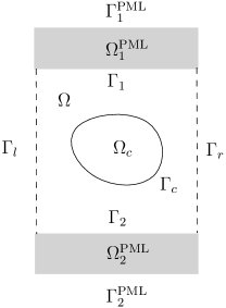
Figure 2: The schematic of the PML problem.

The PML parameters in $\Omega_{k}^{\rm PML}$ are introduced by the complex coordinate stretching (cf. [32]):

$$\tilde{x}_{2}=\varphi(x_{2})=\int_{0}^{x_{2}}s(t){\rm d}t,\quad s(t)=\left\{\begin{aligned} &1&&\text{if}~{}h_{2}\leq t\leq h_{1},\\ &1+{\rm i}\sigma_{0}\left(\frac{t-h_{1}}{\delta_{1}}\right)^{m}&&\text{if}~{}t>h_{1},\\ &1+{\rm i}\sigma_{0}\left(\frac{h_{2}-t}{\delta_{2}}\right)^{m}&&\text{if}~{}t<h_{2},\end{aligned}\right.$$

where $\sigma_{0}$ is a positive constant, and $m\geq 2$ is an integer.

Let $\tilde{u}$ be the solution of the total field for the PML problem in the complex coordinates $\tilde{x}=(x_{1},\tilde{x}_{2})$. It satisfies

$$\left\{\begin{aligned} &\tilde{\Delta}^{2}\tilde{u}-\kappa^{4}\tilde{u}=w&&{\rm in}~{}\Omega^{\rm PML},\\ &\tilde{u}=u^{i},\quad\partial_{\nu}\tilde{u}=\partial_{\nu}u^{i}&&{\rm on}~{}\Gamma_{1}^{\rm PML},\\ &\tilde{u}=0,\quad\partial_{\nu}\tilde{u}=0&&{\rm on}~{}\Gamma_{2}^{\rm PML},\\ \end{aligned}\right.$$ (22)

where $\tilde{\Delta}$ is the Laplacian operator in the complex coordinates and is given by

$$\tilde{\Delta}\tilde{u}=\frac{\partial^{2}\tilde{u}}{\partial x_{1}^{2}}+\frac{\partial^{2}\tilde{u}}{\partial\tilde{x}_{2}^{2}},$$

and

$$w(\tilde{x})=\left\{\begin{aligned} &\tilde{\Delta}^{2}u^{i}-\kappa^{4}u^{i}&&\text{in}~{}\Omega_{1}^{\rm PML},\\ &0&&\text{in}~{}\Omega\setminus\overline{\Omega_{1}^{\rm PML}}.\end{aligned}\right.$$

Here, the complex coordinate variable $\tilde{x}=(x_{1},\tilde{x}_{2})$ is considered to be in $\Omega^{\rm PML}_{k}$ or on $\Gamma_{k}^{\rm PML}$ if $x=(x_{1},\psi(\tilde{x}_{2}))$ is in $\Omega^{\rm PML}_{k}$ or on $\Gamma_{k}^{\rm PML}$, where $\psi$ is the inverse function of $\varphi$, i.e., $x_{2}=\psi(\tilde{x}_{2})=\varphi^{-1}(\tilde{x}_{2})$.

5.2 TBC for the PML problem

To equivalently formulate the PML problem from the domain $\Omega^{\rm PML}$ to the domain $\Omega$, we investigate the TBCs of the PML problem (22) on the interfaces $\Gamma_{k}$.

First, we deduce the TBC on $\Gamma_{1}$. Consider the scattered field

$$\tilde{u}^{s}(x_{1},\varphi(x_{2}))=\tilde{u}(x_{1},\varphi(x_{2}))-u^{i}(x_{1},x_{2}).$$

It follows from (22) that the scattered field $\tilde{u}^{s}$ satisfies

$$\left\{\begin{aligned} &\tilde{\Delta}\tilde{u}^{s}-\kappa^{4}\tilde{u}^{s}=0&&{\rm in}~{}\Omega_{1}^{\rm PML},\\ &\tilde{u}^{s}=\hat{f}_{1},\quad\partial_{\nu}\tilde{u}^{s}=\hat{g}_{1}&&{\rm on}~{}\Gamma_{1},\\ &\tilde{u}^{s}=0,\quad\partial_{\nu}\tilde{u}^{s}=0&&{\rm on}~{}\Gamma_{1}^{\rm PML},\\ \end{aligned}\right.$$ (23)

where $(\tilde{u}^{s},\partial_{\nu}\tilde{u}^{s})=(\hat{f}_{1},\hat{g}_{1})$ are the Dirichlet data for the scattered field $\tilde{u}^{s}$ on $\Gamma_{1}$. As $\hat{f}_{1}$ and $\hat{g}_{1}$ are quasi-periodic functions of $x_{1}$ with a period $\Lambda$, they have the Fourier series expansions

$$\hat{f}_{1}(x_{1})=\sum\limits_{n\in\mathbb{Z}}\hat{f}_{1}^{(n)}e^{{\rm i}\alpha_{n}x_{1}},\quad\hat{g}_{1}(x_{1})=\sum\limits_{n\in\mathbb{Z}}\hat{g}_{1}^{(n)}e^{{\rm i}\alpha_{n}x_{1}}.$$

Since the scattered field $\tilde{u}^{s}$ satisfies $\tilde{\Delta}\tilde{u}^{s}-\kappa^{4}\tilde{u}^{s}=0$ in $\Omega_{1}^{\rm PML}$, we can verify that $\tilde{u}^{s}$ admits the following analytical expression in $\Omega_{1}^{\rm PML}$:

$$\tilde{u}^{s}(x_{1},\tilde{x}_{2}) =\sum\limits_{n\in\mathbb{Z}}\Big{[}W_{1}^{(n)}e^{-{\rm i}\beta_{n}(\tilde{x}_{2}-h_{1})}+V_{1}^{(n)}e^{{\rm i}\beta_{n}(\tilde{x}_{2}-h_{1})}$$

$$\quad+X_{1}^{(n)}e^{\gamma_{n}(\tilde{x}_{2}-h_{1})}+Y_{1}^{(n)}e^{-\gamma_{n}(\tilde{x}_{2}-h_{1})}\Big{]}e^{{\rm i}\alpha_{n}x_{1}}.$$ (24)

Substituting (24) into the boundary conditions in (23), we obtain a linear system of algebraic equations for the Fourier coefficients $W_{1}^{(n)},V_{1}^{(n)},X_{1}^{(n)}$, and $Y_{1}^{(n)}$:

$$\left\{\begin{aligned} &W_{1}^{(n)}+V_{1}^{(n)}+X_{1}^{(n)}+Y_{1}^{(n)}=\hat{f}_{1}^{(n)},\\ &-{\rm i}\beta_{n}W_{1}^{(n)}+{\rm i}\beta_{n}V_{1}^{(n)}+\gamma_{n}X_{1}^{(n)}-\gamma_{n}Y_{1}^{(n)}=\hat{g}_{1}^{(n)},\\ &W_{1}^{(n)}e^{-{\rm i}\beta_{n}\tilde{h}_{1}}+V_{1}^{(n)}e^{{\rm i}\beta_{n}\tilde{h}_{1}}+X_{1}^{(n)}e^{\gamma_{n}\tilde{h}_{1}}+Y_{1}^{(n)}e^{-\gamma_{n}\tilde{h}_{1}}=0,\\ &-{\rm i}\beta_{n}W_{1}^{(n)}e^{-{\rm i}\beta_{n}\tilde{h}_{1}}+{\rm i}\beta_{n}V_{1}^{(n)}e^{{\rm i}\beta_{n}\tilde{h}_{1}}+\gamma_{n}X_{1}^{(n)}e^{\gamma_{n}\tilde{h}_{1}}-\gamma_{n}Y_{1}^{(n)}e^{-\gamma_{n}\tilde{h}_{1}}=0,\end{aligned}\right.$$ (25)

where

$$\tilde{h}_{1}=\varphi(h_{1}+\delta_{1})-h_{1}=\int_{0}^{h_{1}+\delta_{1}}s(t){\rm d}t-h_{1}=\delta_{1}\Big{(}1+\frac{{\rm i}\sigma_{0}}{m+1}\Big{)}.$$ (26)

Through tedious yet straightforward calculations, we solve the linear system (25) and obtain the solutions for the Fourier coefficients:

$$W_{1}^{(n)} =\frac{1}{D^{(n)}_{1}}\bigg{\{}\hat{f}_{1}^{(n)}\Big{[}\left(\gamma_{n}\beta_{n}-{\rm i}\gamma_{n}^{2}\right)e^{2{\rm i}\beta_{n}\tilde{h}_{1}}-2\beta_{n}\gamma_{n}e^{({\rm i}\beta_{n}+\gamma_{n})\tilde{h}_{1}}$$

$$\quad+\left(\gamma_{n}\beta_{n}+{\rm i}\gamma_{n}^{2}\right)e^{2({\rm i}\beta_{n}+\gamma_{n})\tilde{h}_{1}}\Big{]}-\hat{g}_{1}^{(n)}\Big{[}\left(\beta_{n}-{\rm i}\gamma_{n}\right)e^{2{\rm i}\beta_{n}\tilde{h}_{1}}$$

$$\quad+2{\rm i}\gamma_{n}e^{({\rm i}\beta_{n}+\gamma_{n})\tilde{h}_{1}}-\left({\rm i}\gamma_{n}+\beta_{n}\right)e^{2({\rm i}\beta_{n}+\gamma_{n})\tilde{h}_{1}}\Big{]}\bigg{\}},$$

$$V_{1}^{(n)} =\frac{1}{D^{(n)}_{1}}\bigg{\{}\hat{f}_{1}^{(n)}\left[\left(\beta_{n}\gamma_{n}+{\rm i}\gamma_{n}^{2}\right)+\left(\gamma_{n}\beta_{n}-{\rm i}\gamma_{n}^{2}\right)e^{2\gamma_{n}\tilde{h}_{1}}-2\beta_{n}\gamma_{n}e^{({\rm i}\beta_{n}+\gamma_{n})\tilde{h}_{1}}\right]$$

$$\quad-\hat{g}_{1}^{(n)}\left[\left(\beta_{n}+{\rm i}\gamma_{n}\right)-\left(\beta_{n}-{\rm i}\gamma_{n}\right)e^{2\gamma_{n}\tilde{h}_{1}}-2{\rm i}\gamma_{n}e^{({\rm i}\beta_{n}+\gamma_{n})\tilde{h}_{1}}\right]\bigg{\}},$$

$$X_{1}^{(n)} =\frac{1}{D^{(n)}_{1}}\bigg{\{}\hat{f}_{1}^{(n)}\left[(\beta_{n}\gamma_{n}-{\rm i}\beta_{n}^{2})+\left({\rm i}\beta_{n}^{2}+\beta_{n}\gamma_{n}\right)e^{2{\rm i}\beta_{n}\tilde{h}_{1}}-2\beta_{n}\gamma_{n}e^{({\rm i}\beta_{n}+\gamma_{n})\tilde{h}_{1}}\right]$$

$$\quad-\hat{g}_{1}^{(n)}\left[-\left(\beta_{n}+{\rm i}\gamma_{n}\right)-\left(\beta_{n}-{\rm i}\gamma_{n}\right)e^{2{\rm i}\beta_{n}\tilde{h}_{1}}+2\beta_{n}e^{({\rm i}\beta_{n}+\gamma_{n})\tilde{h}_{1}}\right]\bigg{\}},$$

$$Y_{1}^{(n)} =\frac{1}{D^{(n)}_{1}}\bigg{\{}\hat{f}_{1}^{(n)}\Big{[}\left({\rm i}\beta_{n}^{2}+\beta_{n}\gamma_{n}\right)e^{2\gamma_{n}\tilde{h}_{1}}-2\beta_{n}\gamma_{n}e^{({\rm i}\beta_{n}+\gamma_{n})\tilde{h}_{1}}$$

$$\quad+\left(\beta_{n}\gamma_{n}-{\rm i}\beta_{n}^{2}\right)e^{2({\rm i}\beta_{n}+\gamma_{n})\tilde{h}_{1}}\Big{]}-\hat{g}_{1}^{(n)}\Big{[}\left(\beta_{n}-{\rm i}\gamma_{n}\right)e^{2\gamma_{n}\tilde{h}_{1}}$$

$$\quad-2\beta_{n}e^{({\rm i}\beta_{n}+\gamma_{n})\tilde{h}_{1}}+\left({\rm i}\gamma_{n}+\beta_{n}\right)e^{2({\rm i}\beta_{n}+\gamma_{n})\tilde{h}_{1}}\Big{]}\bigg{\}},$$

where the denominator $D^{(n)}_{1}$ is defined as

$$D^{(n)}_{1} =-8\beta_{n}\gamma_{n}e^{({\rm i}\beta_{n}+\gamma_{n})\tilde{h}_{1}}+\left(-{\rm i}\beta_{n}^{2}+{\rm i}\gamma_{n}^{2}+2\beta_{n}\gamma_{n}\right)\big{(}1+e^{2({\rm i}\beta_{n}+\gamma_{n})\tilde{h}_{1}}\big{)}$$

$$\quad+\left({\rm i}\beta_{n}^{2}-{\rm i}\gamma_{n}^{2}+2\beta_{n}\gamma_{n}\right)\big{(}e^{2{\rm i}\beta_{n}\tilde{h}_{1}}+e^{2\gamma_{n}\tilde{h}_{1}}\big{)}.$$ (27)

It is clear to note from (26) that both of the real and imaginary parts of $\tilde{h}_{1}$ are positive. If the thickness of the layer $\delta_{1}$ is sufficiently large, i.e., $\Re\tilde{h}_{1}=\delta_{1}$ is sufficiently large, then the leading term in (5.2) is the one containing $e^{2\gamma_{n}\tilde{h}_{1}}$. A simple calculations yields

$$\left|{\rm i}\beta_{n}^{2}-{\rm i}\gamma_{n}^{2}+2\beta_{n}\gamma_{n}\right|^{2}=|\gamma_{n}+{\rm i}\beta_{n}|^{4}\neq 0\quad\forall\,n\in\mathbb{Z},$$

which ensures that $D^{(n)}_{1}$ is non-zero for sufficiently large $\delta_{1}$.

Substituting (24) into (7), we obtain the TBC of the scattered field $\tilde{u}^{s}$ for the PML problem on $\Gamma_{1}$:

$$N_{1}\tilde{u}^{s}=\hat{T}_{11}^{(1)}\hat{f}_{1}+\hat{T}_{12}^{(1)}\hat{g}_{1},\quad M_{1}\tilde{u}^{s}=\hat{T}_{21}^{(1)}\hat{f}_{1}+\hat{T}_{22}^{(1)}\hat{g}_{1},$$ (28)

where the DtN operators $\hat{T}_{ij}^{(1)},i,j=1,2$ are given by

$$(\hat{T}^{(1)}_{11}\hat{f}_{1})(x_{1}) =-\sum\limits_{n\in\mathbb{Z}}\frac{e^{{\rm i}\alpha_{n}x_{1}}}{D^{(n)}_{1}}\hat{f}_{1}^{(n)}\Big{\{}-\left({\rm i}\beta_{n}^{4}\gamma_{n}-\beta_{n}^{3}\gamma_{n}^{2}+{\rm i}\beta_{n}^{2}\gamma_{n}^{3}-\beta_{n}\gamma_{n}^{4}\right)$$

$$\quad+\left({\rm i}\beta_{n}^{4}\gamma_{n}+\beta_{n}^{3}\gamma_{n}^{2}+{\rm i}\beta_{n}^{2}\gamma_{n}^{3}+\beta_{n}\gamma_{n}^{4}\right)e^{2{\rm i}\beta_{n}\tilde{h}_{1}}$$

$$\quad-\left({\rm i}\beta_{n}^{4}\gamma_{n}+\beta_{n}^{3}\gamma_{n}^{2}+{\rm i}\beta_{n}^{2}\gamma_{n}^{3}\beta_{n}\gamma_{n}^{4}\right)e^{2\gamma_{n}\tilde{h}_{1}}$$

$$\quad+\left({\rm i}\beta_{n}^{4}\gamma_{n}-\beta_{n}^{3}\gamma_{n}^{2}+{\rm i}\beta_{n}^{2}\gamma_{n}^{3}-\beta_{n}\gamma_{n}^{4}\right)e^{2({\rm i}\beta_{n}+\gamma_{n})\tilde{h}_{1}}\Big{\}},$$

$$(\hat{T}^{(1)}_{12}\hat{g}_{1})(x_{1}) =-\sum\limits_{n\in\mathbb{Z}}\frac{e^{{\rm i}\alpha_{n}x_{1}}}{D^{(n)}_{1}}\hat{g}_{1}^{(n)}\bigg{\{}\Big{(}\frac{\rm i}{2}\mu\beta_{n}^{4}+(1-\mu)\beta_{n}^{3}\gamma_{n}+(2-\mu){\rm i}\beta_{n}^{2}\gamma_{n}^{2}$$

$$\quad-(1-\mu)\beta_{n}\gamma_{n}^{3}+\frac{\mu}{2}{\rm i}\gamma_{n}^{4}\Big{)}+\Big{(}-\frac{\rm i}{2}\mu\beta_{n}^{4}+(1-\mu)\beta_{n}^{3}\gamma_{n}-(2-\mu){\rm i}\beta_{n}^{2}\gamma_{n}^{2}$$

$$\quad-(1-\mu)\beta_{n}\gamma_{n}^{3}-\frac{\rm i}{2}\mu\gamma_{n}^{4}\Big{)}e^{2{\rm i}\beta_{n}\tilde{h}_{1}}+\Big{(}-\frac{\rm i}{2}\mu\beta_{n}^{4}+(1-\mu)\beta_{n}^{3}\gamma_{n}$$

$$\quad-(2-\mu){\rm i}\beta_{n}^{2}\gamma_{n}^{2}-(1-\mu)\beta_{n}\gamma_{n}^{3}-\frac{\rm i}{2}\mu\gamma_{n}^{4}\Big{)}e^{2\gamma_{n}\tilde{h}_{1}}$$

$$\quad+(4-4\mu)\left(\beta_{n}\gamma_{n}^{3}-\beta_{n}^{3}\gamma_{n}\right)e^{({\rm i}\beta_{n}+\gamma_{n})\tilde{h}_{1}}+\Big{(}\frac{\rm i}{2}\mu\beta_{n}^{4}+(1-\mu)\beta_{n}^{3}\gamma_{n}$$

$$\quad+(2-\mu){\rm i}\beta_{n}^{2}\gamma_{n}^{2}-(1-\mu)\beta_{n}\gamma_{n}^{3}+\frac{\mu}{2}{\rm i}\gamma_{n}^{4}\Big{)}e^{2({\rm i}\beta_{n}+\gamma_{n})\tilde{h}_{1}}\bigg{\}},$$

$$(\hat{T}_{21}^{(1)}\hat{f}_{1})(x_{1}) =-\sum\limits_{n\in\mathbb{Z}}\frac{e^{{\rm i}\alpha_{n}x_{1}}}{D^{(n)}_{1}}\hat{f}_{1}^{(n)}\bigg{\{}\Big{(}\frac{\rm i}{2}\mu\beta_{n}^{4}+(1-\mu)\beta_{n}^{3}\gamma_{n}+(2-\mu){\rm i}\beta_{n}^{2}\gamma_{n}^{2}$$

$$\quad-(1-\mu)\beta_{n}\gamma_{n}^{3}+\frac{\rm i}{2}\mu\gamma_{n}^{4}\Big{)}+\Big{(}-\frac{\rm i}{2}\mu\beta_{n}^{4}+(1-\mu)\beta_{n}^{3}\gamma_{n}-(2-\mu){\rm i}\beta_{n}^{2}\gamma_{n}^{2}$$

$$\quad-(1-\mu)\beta_{n}\gamma_{n}^{3}-\frac{\rm i}{2}\mu\gamma_{n}^{4}\Big{)}e^{2{\rm i}\beta_{n}\tilde{h}_{1}}+\Big{(}-\frac{\rm i}{2}\mu\beta_{n}^{4}+(1-\mu)\beta_{n}^{3}\gamma_{n}$$

$$\quad-(2-\mu){\rm i}\beta_{n}^{2}\gamma_{n}^{2}-(1-\mu)\beta_{n}\gamma_{n}^{3}-\frac{\rm i}{2}\mu\gamma_{n}^{4}\Big{)}e^{2\gamma_{n}\tilde{h}_{1}}$$

$$\quad+(4-4\mu)\left(\gamma_{n}^{3}\beta_{n}-\beta_{n}^{3}\gamma_{n}\right)e^{({\rm i}\beta_{n}+\gamma_{n})\tilde{h}_{1}}+\Big{(}\frac{\rm i}{2}\mu\beta_{n}^{4}+(1-\mu)\beta_{n}^{3}\gamma_{n}$$

$$\quad+(2-\mu){\rm i}\beta_{n}^{2}\gamma_{n}^{2}-(1-\mu)\beta_{n}\gamma_{n}^{3}+\frac{\rm i}{2}\mu\gamma_{n}^{4}\Big{)}e^{2({\rm i}\beta_{n}+\gamma_{n})\tilde{h}_{1}}\bigg{\}},$$

and

$$(\hat{T}_{22}^{(1)}\hat{g}_{1})(x_{1}) =-\sum\limits_{n\in\mathbb{Z}}\frac{e^{{\rm i}\alpha_{n}x_{1}}}{D^{(n)}_{1}}\hat{g}_{1}^{(n)}\Big{\{}-\left(\beta_{n}^{3}+{\rm i}\beta_{n}^{2}\gamma_{n}+\beta_{n}\gamma_{n}^{2}+{\rm i}\gamma_{n}^{3}\right)$$

$$\quad-\left(\beta_{n}^{3}-{\rm i}\beta_{n}^{2}\gamma_{n}+\beta_{n}\gamma_{n}^{2}-{\rm i}\gamma_{n}^{3}\right)e^{2{\rm i}\beta_{n}\tilde{h}_{1}}$$

$$\quad+\left(\beta_{n}^{3}-{\rm i}\beta_{n}^{2}\gamma_{n}+\beta_{n}\gamma_{n}^{2}-{\rm i}\gamma_{n}^{3}\right)e^{2\gamma_{n}\tilde{h}_{1}}$$

$$\quad+\left(\beta_{n}^{3}+{\rm i}\beta_{n}^{2}\gamma_{n}+\beta_{n}\gamma_{n}^{2}+{\rm i}\gamma_{n}^{3}\right)e^{2({\rm i}\beta_{n}+\gamma_{n})\tilde{h}_{1}}\Big{\}}.$$

Let $(\tilde{u},\partial_{\nu}\tilde{u})=(f_{1},g_{1})$ be the Dirichlet data of the total field $\tilde{u}$ on $\Gamma_{1}$. Utilizing (28) and noting $f_{1}=\hat{f}_{1}+u^{i}$ and $g_{1}=\hat{g}_{1}+\partial_{x_{2}}u^{i}$, the TBC for the total field $\tilde{u}$ on $\Gamma_{1}$ can be formulated as

$$N_{1}\tilde{u}=\hat{T}_{11}^{(1)}f_{1}+\hat{T}_{12}^{(1)}g_{1}+\hat{p}_{1},\quad M_{1}\tilde{u}=\hat{T}_{21}^{(1)}f_{1}+\hat{T}_{22}^{(1)}g_{1}+\hat{p}_{2},$$ (29)

where

$$\hat{p}_{1}(x_{1})=N_{1}u^{i}-\hat{T}_{11}^{(1)}u^{i}-\hat{T}_{12}^{(1)}\partial_{x_{2}}u^{i},\quad\hat{p}_{2}(x_{1})=M_{1}u^{i}-\hat{T}_{21}^{(1)}u^{i}-\hat{T}_{22}^{(1)}\partial_{x_{2}}u^{i}.$$ (30)

The TBC can be similarly deduced on $\Gamma_{2}$. Derived from the biharmonic wave equation in (22), the PML solution $\tilde{u}$ exhibits the following analytical expansion in $\Omega_{2}^{\rm PML}$:

$$\tilde{u}(x_{1},\tilde{x}_{2}) =\sum\limits_{n\in\mathbb{Z}}\Big{[}W_{2}^{(n)}e^{-{\rm i}\beta_{n}(\tilde{x}_{2}-h_{2})}+V_{2}^{(n)}e^{{\rm i}\beta_{n}(\tilde{x}_{2}-h_{2})}$$

$$\quad+X_{2}^{(n)}e^{\gamma_{n}(\tilde{x}_{2}-h_{2})}+Y_{2}^{(n)}e^{-\gamma_{n}(\tilde{x}_{2}-h_{2})}\Big{]}e^{{\rm i}\alpha_{n}x_{1}}.$$ (31)

Substituting (5.2) into the boundary conditions in (22), we obtain a linear system for the Fourier coefficients $W_{2}^{(n)},V_{2}^{(n)},X_{2}^{(n)}$, and $Y_{2}^{(n)}$:

$$\left\{\begin{aligned} &W_{2}^{(n)}+V_{2}^{(n)}+X_{2}^{(n)}+Y_{2}^{(n)}=f_{2}^{(n)},\\ &-{\rm i}\beta_{n}W_{2}^{(n)}+{\rm i}\beta_{n}V_{2}^{(n)}+\gamma_{n}X_{2}^{(n)}-\gamma_{n}Y_{2}^{(n)}=-g_{2}^{(n)},\\ &W_{2}^{(n)}e^{-{\rm i}\beta_{n}\tilde{h}_{2}}+V_{2}^{(n)}e^{{\rm i}\beta_{n}\tilde{h}_{2}}+X_{2}^{(n)}e^{\gamma_{n}\tilde{h}_{2}}+Y_{2}^{(n)}e^{-\gamma_{n}\tilde{h}_{2}}=0,\\ &-{\rm i}\beta_{n}W_{2}^{(n)}e^{-{\rm i}\beta_{n}\tilde{h}_{2}}+{\rm i}\beta_{n}V_{2}^{(n)}e^{{\rm i}\beta_{n}\tilde{h}_{2}}+\gamma_{n}X_{2}^{(n)}e^{\gamma_{n}\tilde{h}_{2}}-\gamma_{n}Y_{2}^{(n)}e^{-\gamma_{n}\tilde{h}_{2}}=0,\end{aligned}\right.$$ (32)

where $(\tilde{u},\partial_{\nu}\tilde{u})=(f_{2},g_{2})$ represent the Dirichlet data of the total field on $\Gamma_{2}$ and have the Fourier series expansions

$$f_{2}=\sum\limits_{n\in\mathbb{Z}}f_{2}^{(n)}e^{{\rm i}\alpha_{n}x_{1}},\quad g_{2}=\sum\limits_{n\in\mathbb{Z}}g_{2}^{(n)}e^{{\rm i}\alpha_{n}x_{1}},$$

and

$$\tilde{h}_{2}:=\varphi(h_{2}-\delta_{2})-h_{2}=\int_{0}^{h_{2}-\delta_{2}}s(t){\rm d}t-h_{2}=-\delta_{2}\left(1+\frac{{\rm i}\sigma_{0}}{m+1}\right).$$ (33)

Upon solving the linear system (32), we have

$$W_{2}^{(n)} =\frac{1}{D^{(n)}_{2}}\bigg{\{}f_{2}^{(n)}\Big{[}\left(\gamma_{n}\beta_{n}-{\rm i}\gamma_{n}^{2}\right)e^{2{\rm i}\beta_{n}\tilde{h}_{2}}-2\beta_{n}\gamma_{n}e^{({\rm i}\beta_{n}+\gamma_{n})\tilde{h}_{2}}$$

$$\quad+\left(\gamma_{n}\beta_{n}+{\rm i}\gamma_{n}^{2}\right)e^{2({\rm i}\beta_{n}+\gamma_{n})\tilde{h}_{2}}\Big{]}+g_{2}^{(n)}\Big{[}\left(\beta_{n}-{\rm i}\gamma_{n}\right)e^{2{\rm i}\beta_{n}\tilde{h}_{2}}$$

$$\quad+2{\rm i}\gamma_{n}e^{({\rm i}\beta_{n}+\gamma_{n})\tilde{h}_{2}}-\left({\rm i}\gamma_{n}+\beta_{n}\right)e^{2({\rm i}\beta_{n}+\gamma_{n})\tilde{h}_{2}}\Big{]}\bigg{\}},$$

$$V_{2}^{(n)} =\frac{1}{D^{(n)}_{2}}\bigg{\{}f_{2}^{(n)}\left[\left(\beta_{n}\gamma_{n}+{\rm i}\gamma_{n}^{2}\right)+\left(\gamma_{n}\beta_{n}-{\rm i}\gamma_{n}^{2}\right)e^{2\gamma_{n}\tilde{h}_{2}}-2\beta_{n}\gamma_{n}e^{({\rm i}\beta_{n}+\gamma_{n})\tilde{h}_{2}}\right]$$

$$\quad+g_{2}^{(n)}\left[\left(\beta_{n}+{\rm i}\gamma_{n}\right)-\left(\beta_{n}-{\rm i}\gamma_{n}\right)e^{2\gamma_{n}\tilde{h}_{2}}-2{\rm i}\gamma_{n}e^{({\rm i}\beta_{n}+\gamma_{n})\tilde{h}_{2}}\right]\bigg{\}},$$

$$X_{2}^{(n)} =\frac{1}{D^{(n)}_{2}}\bigg{\{}f_{2}^{(n)}\left[\left(\beta_{n}\gamma_{n}-{\rm i}\beta_{n}^{2}\right)+\left({\rm i}\beta_{n}^{2}+\beta_{n}\gamma_{n}\right)e^{2{\rm i}\beta_{n}\tilde{h}_{2}}-2\beta_{n}\gamma_{n}e^{({\rm i}\beta_{n}+\gamma_{n})\tilde{h}_{2}}\right]$$

$$\quad+g_{2}^{(n)}\left[-\left(\beta_{n}+{\rm i}\gamma_{n}\right)-\left(\beta_{n}-{\rm i}\gamma_{n}\right)e^{2{\rm i}\beta_{n}\tilde{h}_{2}}+2\beta_{n}e^{({\rm i}\beta_{n}+\gamma_{n})\tilde{h}_{2}}\right]\bigg{\}},$$

$$Y_{2}^{(n)} =\frac{1}{D^{(n)}_{2}}\bigg{\{}f_{2}^{(n)}\Big{[}\left({\rm i}\beta_{n}^{2}+\beta_{n}\gamma_{n}\right)e^{2\gamma_{n}\tilde{h}_{2}}-2\beta_{n}\gamma_{n}e^{({\rm i}\beta_{n}+\gamma_{n})\tilde{h}_{2}}$$

$$\quad+\left(\beta_{n}\gamma_{n}-{\rm i}\beta_{n}^{2}\right)e^{2({\rm i}\beta_{n}+\gamma_{n})\tilde{h}_{2}}\Big{]}+g_{2}^{(n)}\Big{[}\left(\beta_{n}-{\rm i}\gamma_{n}\right)e^{2\gamma_{n}\tilde{h}_{2}}$$

$$\quad-2\beta_{n}e^{({\rm i}\beta_{n}+\gamma_{n})\tilde{h}_{2}}+\left({\rm i}\gamma_{n}+\beta_{n}\right)e^{2({\rm i}\beta_{n}+\gamma_{n})\tilde{h}_{2}}\Big{]}\bigg{\}},$$

where the denominator $D^{(n)}_{2}$ is given by

$$D^{(n)}_{2} =-8\beta_{n}\gamma_{n}e^{({\rm i}\beta_{n}+\gamma_{n})\tilde{h}_{2}}+\left(-{\rm i}\beta_{n}^{2}+{\rm i}\gamma_{n}^{2}+2\beta_{n}\gamma_{n}\right)\big{(}1+e^{2({\rm i}\beta_{n}+\gamma_{n})\tilde{h}_{2}}\big{)}$$ (34)

$$\quad+\left({\rm i}\beta_{n}^{2}-{\rm i}\gamma_{n}^{2}+2\beta_{n}\gamma_{n}\right)\big{(}e^{2{\rm i}\beta_{n}\tilde{h}_{2}}+e^{2\gamma_{n}\tilde{h}_{2}}\big{)}.$$

By (33), both of the real and imaginary parts of $\tilde{h}_{2}$ are negative. If the thickness of the layer $\delta_{2}$ is sufficiently large, i.e., $-\Re\tilde{h}_{2}=\delta_{2}$ is sufficiently large, then the leading term in (34) is the one containing $e^{2{\rm i}\beta_{n}\tilde{h}_{2}}$. Observing $|{\rm i}\beta_{n}^{2}-{\rm i}\gamma_{n}^{2}+2\beta_{n}\gamma_{n}|^{2}=|\gamma_{n}+{\rm i}\beta_{n}|^{4}\neq 0$ for any $n\in\mathbb{Z}$, we deduce that the denominator $D^{(2)}_{n}$ in non-zero for sufficiently large $\delta_{2}$.

Substituting (5.2) into (14), we obtain the TBC for the PML problem on $\Gamma_{2}$:

$$N_{2}\tilde{u}=\hat{T}_{11}^{(2)}f_{2}+\hat{T}_{12}^{(2)}g_{2},\quad M_{2}\tilde{u}=\hat{T}_{21}^{(2)}f_{2}+\hat{T}_{22}^{(2)}g_{2},$$ (35)

where the DtN operators $\hat{T}_{ij}^{(2)},i,j=1,2$ are defined as

$$(\hat{T}^{(2)}_{11}f_{2})(x_{1}) =-\sum\limits_{n\in\mathbb{Z}}\frac{e^{{\rm i}\alpha_{n}x_{1}}}{D^{(2)}_{n}}f_{2}^{(n)}\Big{\{}\left({\rm i}\beta_{n}^{4}\gamma_{n}-\beta_{n}^{3}\gamma_{n}^{2}+{\rm i}\beta_{n}^{2}\gamma_{n}^{3}-\beta_{n}\gamma_{n}^{4}\right)$$

$$\quad-\left({\rm i}\beta_{n}^{4}\gamma_{n}+\beta_{n}^{3}\gamma_{n}^{2}+{\rm i}\beta_{n}^{2}\gamma_{n}^{3}+\beta_{n}\gamma_{n}^{4}\right)e^{2{\rm i}\beta_{n}\tilde{h}_{2}}$$

$$\quad+\left({\rm i}\beta_{n}^{4}\gamma_{n}+\beta_{n}^{3}\gamma_{n}^{2}+{\rm i}\beta_{n}^{2}\gamma_{n}^{3}+\beta_{n}\gamma_{n}^{4}\right)e^{2\gamma_{n}\tilde{h}_{2}}$$

$$\quad-\left({\rm i}\beta_{n}^{4}\gamma_{n}-\beta_{n}^{3}\gamma_{n}^{2}+{\rm i}\beta_{n}^{2}\gamma_{n}^{3}-\beta_{n}\gamma_{n}^{4}\right)e^{2({\rm i}\beta_{n}+\gamma_{n})\tilde{h}_{2}}\Big{\}},$$

$$(\hat{T}^{(2)}_{12}g_{2})(x_{1}) =-\sum\limits_{n\in\mathbb{Z}}\frac{e^{{\rm i}\alpha_{n}x_{1}}}{D^{(2)}_{n}}g_{2}^{(n)}\bigg{\{}\Big{(}\frac{\rm i}{2}\mu\beta_{n}^{4}+(1-\mu)\beta_{n}^{3}\gamma_{n}+(2-\mu){\rm i}\beta_{n}^{2}\gamma_{n}^{2}$$

$$\quad-(1-\mu)\beta_{n}\gamma_{n}^{3}+\frac{\mu}{2}{\rm i}\gamma_{n}^{4}\Big{)}+\Big{(}-\frac{\rm i}{2}\mu\beta_{n}^{4}+(1-\mu)\beta_{n}^{3}\gamma_{n}-(2-\mu){\rm i}\beta_{n}^{2}\gamma_{n}^{2}$$

$$\quad-(1-\mu)\beta_{n}\gamma_{n}^{3}-\frac{\rm i}{2}\mu\gamma_{n}^{4}\Big{)}e^{2{\rm i}\beta_{n}\tilde{h}_{2}}+\Big{(}-\frac{\rm i}{2}\mu\beta_{n}^{4}+(1-\mu)\beta_{n}^{3}\gamma_{n}$$

$$\quad-(2-\mu){\rm i}\beta_{n}^{2}\gamma_{n}^{2}-(1-\mu)\beta_{n}\gamma_{n}^{3}-\frac{\rm i}{2}\mu\gamma_{n}^{4}\Big{)}e^{2\gamma_{n}\tilde{h}_{2}}$$

$$\quad+(4-4\mu)\left(\beta_{n}\gamma_{n}^{3}-\beta_{n}^{3}\gamma_{n}\right)e^{({\rm i}\beta_{n}+\gamma_{n})\tilde{h}_{2}}+\Big{(}\frac{\rm i}{2}\mu\beta_{n}^{4}+(1-\mu)\beta_{n}^{3}\gamma_{n}$$

$$\quad+(2-\mu){\rm i}\beta_{n}^{2}\gamma_{n}^{2}-(1-\mu)\beta_{n}\gamma_{n}^{3}+\frac{\mu}{2}{\rm i}\gamma_{n}^{4}\Big{)}e^{2({\rm i}\beta_{n}+\gamma_{n})\tilde{h}_{2}}\bigg{\}},$$

$$(\hat{T}_{21}^{(2)}(n)f_{2})(x_{1}) =-\sum\limits_{n\in\mathbb{Z}}\frac{e^{{\rm i}\alpha_{n}x_{1}}}{D^{(2)}_{n}}f_{2}^{(n)}\bigg{\{}\Big{(}\frac{\rm i}{2}\mu\beta_{n}^{4}+(1-\mu)\beta_{n}^{3}\gamma_{n}+(2-\mu){\rm i}\beta_{n}^{2}\gamma_{n}^{2}$$

$$\quad-(1-\mu)\beta_{n}\gamma_{n}^{3}+\frac{\rm i}{2}\mu\gamma_{n}^{4}\Big{)}+\Big{(}-\frac{\rm i}{2}\mu\beta_{n}^{4}+(1-\mu)\beta_{n}^{3}\gamma_{n}-(2-\mu){\rm i}\beta_{n}^{2}\gamma_{n}^{2}$$

$$\quad-(1-\mu)\beta_{n}\gamma_{n}^{3}-\frac{\rm i}{2}\mu\gamma_{n}^{4}\Big{)}e^{2{\rm i}\beta_{n}\tilde{h}_{2}}+\Big{(}-\frac{\rm i}{2}\mu\beta_{n}^{4}+(1-\mu)\beta_{n}^{3}\gamma_{n}$$

$$\quad-(2-\mu){\rm i}\beta_{n}^{2}\gamma_{n}^{2}-(1-\mu)\beta_{n}\gamma_{n}^{3}-\frac{\rm i}{2}\mu\gamma_{n}^{4}\Big{)}e^{2\gamma_{n}\tilde{h}_{2}}$$

$$\quad+(4-4\mu)\left(\gamma_{n}^{3}\beta_{n}-\beta_{n}^{3}\gamma_{n}\right)e^{({\rm i}\beta_{n}+\gamma_{n})\tilde{h}_{2}}+\Big{(}\frac{\rm i}{2}\mu\beta_{n}^{4}+(1-\mu)\beta_{n}^{3}\gamma_{n}$$

$$\quad+(2-\mu){\rm i}\beta_{n}^{2}\gamma_{n}^{2}-(1-\mu)\beta_{n}\gamma_{n}^{3}+\frac{\rm i}{2}\mu\gamma_{n}^{4}\Big{)}e^{2({\rm i}\beta_{n}+\gamma_{n})\tilde{h}_{2}}\bigg{\}},$$

and

$$(\hat{T}_{22}^{(2)}(n)g_{2})(x_{1}) =-\sum\limits_{n\in\mathbb{Z}}\frac{e^{{\rm i}\alpha_{n}x_{1}}}{D^{(2)}_{n}}g_{2}^{(n)}\Big{\{}\left(\beta_{n}^{3}+{\rm i}\beta_{n}^{2}\gamma_{n}+\beta_{n}\gamma_{n}^{2}+{\rm i}\gamma_{n}^{3}\right)$$

$$\quad+\left(\beta_{n}^{3}-{\rm i}\beta_{n}^{2}\gamma_{n}+\beta_{n}\gamma_{n}^{2}-{\rm i}\gamma_{n}^{3}\right)e^{2{\rm i}\beta_{n}\tilde{h}_{2}}$$

$$\quad-\left(\beta_{n}^{3}-{\rm i}\beta_{n}^{2}\gamma_{n}+\beta_{n}\gamma_{n}^{2}-{\rm i}\gamma_{n}^{3}\right)e^{2\gamma_{n}\tilde{h}_{2}}$$

$$\quad-\left(\beta_{n}^{3}+{\rm i}\beta_{n}^{2}\gamma_{n}+\beta_{n}\gamma_{n}^{2}+{\rm i}\gamma_{n}^{3}\right)e^{2({\rm i}\beta_{n}+\gamma_{n})\tilde{h}_{2}}\Big{\}}.$$

Lemma 5.

Assuming that the thickness of the PML layers $\delta_{k}$ for $k=1,2$ are sufficiently large, the DtN operators $\hat{T}^{(k)}_{11}:H^{3/2}(\Gamma_{k})\to H^{-3/2}(\Gamma_{k})$, $\hat{T}^{(k)}_{12}:H^{1/2}(\Gamma_{k})\to H^{-3/2}(\Gamma_{k})$, $\hat{T}^{(k)}_{21}:H^{3/2}(\Gamma_{k})\to H^{-1/2}(\Gamma_{k})$, and $\hat{T}^{(k)}_{22}:H^{1/2}(\Gamma_{k})\to H^{-1/2}(\Gamma_{k})$ are bounded.

Proof.

It is sufficient to present the results for the DtN operators on $\Gamma_{1}$, as the corresponding outcomes can be similarly established for the DtN operators on $\Gamma_{2}$.

As demonstrated in the derivation of the TBC on $\Gamma_{1}$, when the thickness of the PML region is sufficiently large, the term containing $e^{2\gamma_{n}\tilde{h}_{1}}$ is dominant in both the denominator and the numerator. Noting (16), i.e., $\beta_{n}\sim\alpha_{n}$ and $\gamma_{n}\sim\alpha_{n}$ as $n\to\infty$, we assert that for any function $f\in H^{3/2}(\Gamma_{1})$

$$\|\hat{T}_{11}^{(1)}f\|^{2}_{H^{-3/2}(\Gamma_{1})} \lesssim\sum\limits_{n\in\mathbb{Z}}(1+\alpha_{n}^{2})^{-3/2}\left|\frac{f^{(n)}}{D_{1}^{(n)}}\left({\rm i}\beta_{n}^{4}\gamma_{n}+\beta_{n}^{3}\gamma_{n}^{2}+{\rm i}\beta_{n}^{2}\gamma_{n}^{3}+\beta_{n}\gamma_{n}^{4}\right)e^{2\gamma_{n}\tilde{h}_{1}}\right|^{2}$$

$$\lesssim\sum\limits_{n\in\mathbb{Z}}(1+\alpha_{n}^{2})^{-3/2}\left|\frac{\left({\rm i}\beta_{n}^{4}\gamma_{n}+\beta_{n}^{3}\gamma_{n}^{2}+{\rm i}\beta_{n}^{2}\gamma_{n}^{3}+\beta_{n}\gamma_{n}^{4}\right)e^{2\gamma_{n}\tilde{h}_{1}}}{\left({\rm i}\beta_{n}^{2}-{\rm i}\gamma_{n}^{2}+2\beta_{n}\gamma_{n}\right)e^{2\gamma_{n}\tilde{h}_{1}}}\right|^{2}|f^{(n)}|^{2}$$

$$\lesssim\sum\limits_{n\in\mathbb{Z}}(1+\alpha_{n}^{2})^{3/2}|f^{(n)}|^{2}=\|f\|^{2}_{H^{3/2}(\Gamma_{1})},$$

and

$$\|\hat{T}_{21}^{(1)}f\|^{2}_{H^{-1/2}(\Gamma_{1})} \lesssim\sum\limits_{n\in\mathbb{Z}}(1+\alpha_{n}^{2})^{-1/2}$$

$$\times\left|\frac{f^{(n)}}{D_{1}^{(n)}}\Big{(}-\frac{\rm i}{2}\mu\beta_{n}^{4}+(1-\mu)\beta_{n}^{3}\gamma_{n}-(2-\mu){\rm i}\beta_{n}^{2}\gamma_{n}^{2}-(1-\mu)\beta_{n}\gamma_{n}^{3}-\frac{\rm i}{2}\mu\gamma_{n}^{4}\Big{)}e^{2\gamma_{n}\tilde{h}_{1}}\right|^{2}$$

$$\lesssim\sum\limits_{n\in\mathbb{Z}}(1+\alpha_{n}^{2})^{-1/2}$$

$$\times\left|\frac{-\frac{\rm i}{2}\mu\beta_{n}^{4}+(1-\mu)\beta_{n}^{3}\gamma_{n}-(2-\mu){\rm i}\beta_{n}^{2}\gamma_{n}^{2}-(1-\mu)\beta_{n}\gamma_{n}^{3}-\frac{\rm i}{2}\mu\gamma_{n}^{4}}{{\rm i}\beta_{n}^{2}-{\rm i}\gamma_{n}^{2}+2\beta_{n}\gamma_{n}}\right|^{2}|f^{(n)}|^{2}$$

$$\lesssim\sum\limits_{n\in\mathbb{Z}}(1+\alpha_{n}^{2})^{3/2}|f^{(n)}|^{2}=\|f\|^{2}_{H^{3/2}(\Gamma_{1})}.$$

Similarly, we have that for any function $f\in H^{1/2}(\Gamma_{1})$

$$\|\hat{T}_{12}^{(1)}f\|^{2}_{H^{-3/2}(\Gamma_{1})} \lesssim\sum\limits_{n\in\mathbb{Z}}(1+\alpha_{n}^{2})^{-3/2}$$

$$\times\left|\frac{f^{(n)}}{D_{1}^{(n)}}\Big{(}-\frac{\rm i}{2}\mu\beta_{n}^{4}+(1-\mu)\beta_{n}^{3}\gamma_{n}-(2-\mu){\rm i}\beta_{n}^{2}\gamma_{n}^{2}-(1-\mu)\beta_{n}\gamma_{n}^{3}-\frac{\rm i}{2}\mu\gamma_{n}^{4}\Big{)}e^{2\gamma_{n}\tilde{h}_{1}}\right|^{2}$$

$$\lesssim\sum\limits_{n\in\mathbb{Z}}(1+\alpha_{n}^{2})^{-3/2}$$

$$\times\left|\frac{-\frac{\rm i}{2}\mu\beta_{n}^{4}+(1-\mu)\beta_{n}^{3}\gamma_{n}-(2-\mu){\rm i}\beta_{n}^{2}\gamma_{n}^{2}-(1-\mu)\beta_{n}\gamma_{n}^{3}-\frac{\rm i}{2}\mu\gamma_{n}^{4}}{{\rm i}\beta_{n}^{2}-{\rm i}\gamma_{n}^{2}+2\beta_{n}\gamma_{n}}\right|^{2}|f^{(n)}|^{2}$$

$$\lesssim\sum\limits_{n\in\mathbb{Z}}(1+\alpha_{n}^{2})^{1/2}|f^{(n)}|^{2}=\|f\|^{2}_{H^{1/2}(\Gamma_{1})},$$

and

$$\|\hat{T}_{22}^{(1)}f\|^{2}_{H^{-1/2}(\Gamma_{1})} \lesssim\sum\limits_{n\in\mathbb{Z}}(1+\alpha_{n}^{2})^{-1/2}\left|\frac{f^{(n)}}{D_{1}^{(n)}}\left(\beta_{n}^{3}-{\rm i}\beta_{n}^{2}\gamma_{n}+\beta_{n}\gamma_{n}^{2}-{\rm i}\gamma_{n}^{3}\right)e^{2\gamma_{n}\tilde{h}_{1}}\right|^{2}$$

$$\lesssim\sum\limits_{n\in\mathbb{Z}}(1+\alpha_{n}^{2})^{-1/2}\left|\frac{\left(\beta_{n}^{3}-{\rm i}\beta_{n}^{2}\gamma_{n}+\beta_{n}\gamma_{n}^{2}-{\rm i}\gamma_{n}^{3}\right)e^{2\gamma_{n}\tilde{h}_{1}}}{\left({\rm i}\beta_{n}^{2}-{\rm i}\gamma_{n}^{2}+2\beta_{n}\gamma_{n}\right)e^{2\gamma_{n}\tilde{h}_{1}}}\right|^{2}|f^{(n)}|^{2}$$

$$\lesssim\sum\limits_{n\in\mathbb{Z}}(1+\alpha_{n}^{2})^{1/2}|f^{(n)}|^{2}=\|f\|^{2}_{H^{1/2}(\Gamma_{1})},$$

which complete the proof. ∎

The following lemma addresses the error estimates of the DtN operators between the PML problem and the original scattering problem.

Lemma 6.

Let

$$\Delta^{-}=\min_{n\in\mathbb{Z}}\left\{\Re(\beta_{n})>0\right\},\quad\Delta^{+}=\min_{n\in\mathbb{Z}}\left\{\Im(\beta_{n})>0\right\}.$$

For $k=1,2$, if the thickness of the PML region $\delta_{k}$ is sufficiently large, then the following estimates hold for any $f\in H^{3/2}(\Gamma_{k})$:

$$\|(\hat{T}_{11}^{(k)}-T_{11}^{(k)})f\|_{H^{-3/2}(\Gamma_{k})} \lesssim\Theta\|f\|_{H^{3/2}(\Gamma_{k})},$$

$$\|(\hat{T}_{21}^{(k)}-T_{21}^{(k)})f\|_{H^{-1/2}(\Gamma_{k})} \lesssim\Theta\|f\|_{H^{3/2}(\Gamma_{k})},$$

and the following estimates hold for any $f\in H^{1/2}(\Gamma_{k})$:

$$\|(\hat{T}_{12}^{(k)}-T_{12}^{(k)})f\|_{H^{-3/2}(\Gamma_{k})} \lesssim\Theta\|f\|_{H^{1/2}(\Gamma_{k})},$$

$$\|(\hat{T}_{22}^{(k)}-T_{22}^{(k)})f\|_{H^{-1/2}(\Gamma_{k})} \lesssim\Theta\|f\|_{H^{1/2}(\Gamma_{k})},$$

where

$$\Theta=\max\Big{\{}e^{-\frac{2\delta_{k}\sigma_{0}}{m+1}\Delta^{-}},e^{-2\delta_{k}(\kappa^{2}+\alpha^{2})^{1/2}},e^{-2\delta_{k}\Delta^{+}}\Big{\}}.$$ (36)

Proof.

Given the similarity in proof, we only present the details of the error estimate between $\hat{T}_{11}^{(1)}$ and $T_{11}^{(1)}$, with the understanding that the results for the other operators can be obtained in the same manner.

It follows from (28) and (8) that

$$(T_{11}^{(1)}-\hat{T}_{11}^{(1)})f=\sum\limits_{n\in\mathbb{Z}}\frac{e^{{\rm i}\alpha_{n}x}}{D^{(n)}_{1}}f_{1}^{(n)}\Big{\{}\left(-2{\rm i}\beta_{n}^{4}\gamma_{n}+4\beta_{n}^{3}\gamma_{n}^{2}+2{\rm i}\beta_{n}^{2}\gamma_{n}^{3}\right)$$

$$\quad+\left(2{\rm i}\beta_{n}^{4}\gamma_{n}+2\beta_{n}^{3}\gamma_{n}^{2}+2{\rm i}\beta_{n}^{2}\gamma_{n}^{3}+2\beta_{n}\gamma_{n}^{4}\right)e^{2{\rm i}\beta_{n}\tilde{h}_{1}}-\left(8{\rm i}\beta_{n}^{2}\gamma_{n}^{3}+\beta_{n}^{3}\gamma_{n}^{2}\right)e^{({\rm i}\beta_{n}+\gamma_{n})\tilde{h}_{1}}$$

$$\quad+\left(2\beta_{n}^{3}\gamma_{n}^{2}+4{\rm i}\beta_{n}^{2}\gamma_{n}^{3}-2\beta_{n}\gamma_{n}^{4}\right)e^{2({\rm i}\beta_{n}+\gamma_{n})\tilde{h}_{1}}\Big{\}}.$$

When $\delta_{1}$ is sufficiently large, the dominant term in the denominator is the one involving $e^{2\gamma_{n}\tilde{h}_{1}}$, which has a coefficient of ${\rm i}\beta_{n}^{2}-{\rm i}\gamma_{n}^{2}+2\beta_{n}\gamma_{n}$. The dominant terms in the numerator are either the constant term or the one that contains $e^{2({\rm i}\beta_{n}+\gamma_{n})\tilde{h}_{1}}$. By the choice of PML parameters given in (26), a straightforward calculation yields

$$2\gamma_{h}\tilde{h}_{1}=2\delta_{1}\left(1+\frac{{\rm i}\sigma_{0}}{m+1}\right)(\kappa^{2}+\alpha_{n}^{2})^{1/2}=2\delta_{1}(\kappa^{2}+\alpha_{n}^{2})^{1/2}+\frac{2{\rm i}\delta_{1}\sigma_{0}}{m+1}(\kappa^{2}+\alpha_{n}^{2})^{1/2},$$

and

$$2{\rm i}\beta_{n}\tilde{h}_{1}=\left\{\begin{aligned} &2{\rm i}\delta_{1}\left(1+\frac{{\rm i}\sigma_{0}}{m+1}\right)(\kappa^{2}-\alpha_{n}^{2})^{1/2}\\ &\hskip 28.45274pt=-\frac{2\delta_{1}\sigma_{0}}{m+1}(\kappa^{2}-\alpha_{n}^{2})^{1/2}+2{\rm i}\delta_{1}(\kappa^{2}-\alpha_{n}^{2})^{1/2}\quad\text{if}~{}|\alpha_{n}|<\kappa,\\ &-2\delta_{1}\left(1+\frac{{\rm i}\sigma_{0}}{m+1}\right)(\alpha_{n}^{2}-\kappa^{2})^{1/2}\\ &\hskip 28.45274pt=-2\delta_{1}(\alpha_{n}^{2}-\kappa^{2})^{1/2}-\frac{2{\rm i}\delta_{1}\sigma_{0}}{m+1}(\alpha_{n}^{2}-\kappa^{2})^{1/2}\quad\text{if}~{}|\alpha_{n}|>\kappa.\end{aligned}\right.$$

Then we obtain

$$\|(T_{11}^{(1)}-\hat{T}_{11}^{(1)})f\|^{2}_{H^{-3/2}(\Gamma_{1})}\lesssim\sum\limits_{n\in\mathbb{Z}}(1+\alpha_{n}^{2})^{-3/2}\Bigg{(}\bigg{|}\frac{-2{\rm i}\beta_{n}^{4}\gamma_{n}+4\beta_{n}^{3}\gamma_{n}^{2}+2{\rm i}\beta_{n}^{2}\gamma_{n}^{3}}{\left({\rm i}\beta_{n}^{2}-{\rm i}\gamma_{n}^{2}+2\beta_{n}\gamma_{n}\right)e^{2\gamma_{n}\tilde{h}_{1}}}\bigg{|}^{2}$$

$$\qquad+\bigg{|}\frac{\left(2\beta_{n}^{3}\gamma_{n}^{2}+4{\rm i}\beta_{n}^{2}\gamma_{n}^{3}-2\beta_{n}\gamma_{n}^{4}\right)e^{2({\rm i}\beta_{n}+\gamma_{n})\tilde{h}_{1}}}{\left({\rm i}\beta_{n}^{2}-{\rm i}\gamma_{n}^{2}+2\beta_{n}\gamma_{n}\right)e^{2\gamma_{n}\tilde{h}_{1}}}\bigg{|}^{2}\Bigg{)}|f_{1}^{(n)}|^{2}$$

$$\lesssim\sum\limits_{n\in\mathbb{Z}}(1+\alpha_{n}^{2})^{3/2}\left(e^{-4\delta_{1}(\kappa^{2}+\alpha_{n}^{2})^{1/2}}+e^{-\frac{4\delta_{1}\sigma_{0}}{m+1}|\kappa^{2}-\alpha_{n}^{2}|^{1/2}}+e^{-4\delta_{1}|\alpha_{n}^{2}-\kappa^{2}|^{1/2}}\right)|f_{1}^{(n)}|^{2}$$

$$\lesssim\Theta\|f\|_{H^{3/2}(\Gamma_{1})},$$

which completes the proof. ∎

It is evident from Lemma 6 that the DtN operators of the PML problem exhibit exponential convergence in the operator norm to the DtN operators of the original scattering problem. This convergence is a crucial factor contributing to the exponential convergence of the PML solution towards the solution of the original scattering problem.

5.3 Convergence analysis

By employing the TBCs for the PML problem as given in (29) and (35), the PML problem (22) can be reformulated equivalently in the domain $\Omega$:

$$\left\{\begin{aligned} &\Delta^{2}u^{\rm PML}-\kappa^{4}u^{\rm PML}=0&&{\rm in}~{}\Omega,\\ &u^{\rm PML}=0,\quad\partial_{\nu}u^{\rm PML}=0&&{\rm on}~{}\Gamma_{c},\\ &N_{1}u^{\rm PML}=\hat{T}_{11}^{(1)}f_{1}+\hat{T}_{12}^{(1)}g_{1}+\hat{p}_{1}&&{\rm on}~{}\Gamma_{1},\\ &M_{1}u^{\rm PML}=\hat{T}_{21}^{(1)}f_{1}+\hat{T}_{22}^{(1)}g_{1}+\hat{p}_{2}&&{\rm on}~{}\Gamma_{1},\\ &N_{2}u^{\rm PML}=\hat{T}_{11}^{(2)}f_{2}+\hat{T}_{12}^{(2)}g_{2}&&{\rm on}~{}\Gamma_{2},\\ &M_{2}u^{\rm PML}=\hat{T}_{21}^{(2)}f_{2}+\hat{T}_{22}^{(2)}g_{2}&&{\rm on}~{}\Gamma_{2},\end{aligned}\right.$$ (37)

where $\hat{p}_{1}$ and $\hat{p}_{2}$ are given in (30), $(f_{k},g_{k})$ represent the Dirichlet data of the total field $u^{\rm PML}$ on $\Gamma_{k}$ for $k=1,2$.

The variational problem of (37) is to find $u^{\rm PML}\in H_{{\rm qp},\Gamma_{c}}^{2}(\Omega)$ such that

$$a^{\rm PML}(u^{\rm PML},v)=\int_{\Gamma_{1}}\left(\hat{p}_{1}\bar{v}+\hat{p}_{2}\partial_{\nu}\bar{v}\right){\rm d}s\quad\forall\,v\in H_{{\rm qp},\Gamma_{c}}^{2}(\Omega),$$ (38)

where the sesquilinear form $a^{\rm PML}(u,v):H_{{\rm qp},\Gamma_{c}}^{2}(\Omega)\times H_{{\rm qp},\Gamma_{c}}^{2}(\Omega)\rightarrow\mathbb{C}$ is defined as

$$a^{\rm PML}(u,v)=\int_{\Omega}\bigg{[}\mu\Delta u\Delta\bar{v}+(1-\mu)\sum\limits_{i,j=1}^{2}\frac{\partial^{2}u}{\partial x_{i}\partial x_{j}}\frac{\partial^{2}\bar{v}}{\partial x_{i}\partial x_{j}}-\kappa^{4}u\bar{v}\bigg{]}{\rm d}x$$

$$-\sum_{k=1}^{2}\int_{\Gamma_{k}}(\mathbb{\hat{T}}^{(k)}\boldsymbol{u})\cdot\overline{\boldsymbol{v}}{\rm d}s.$$ (39)

with $\boldsymbol{u},\boldsymbol{v}$, and $\mathbb{\hat{T}}^{(k)}$ given by

$$\boldsymbol{u}=\begin{bmatrix}u\\ \partial_{\nu}u\end{bmatrix},\quad\boldsymbol{v}=\begin{bmatrix}v\\ \partial_{\nu}v\end{bmatrix},\quad\mathbb{\hat{T}}^{(k)}=\begin{bmatrix}{\hat{T}}_{11}^{(k)}&{\hat{T}}_{12}^{(k)}\\[5.0pt] {\hat{T}}_{21}^{(k)}&{\hat{T}}_{22}^{(k)}\end{bmatrix}.$$

Theorem 2.

Assuming that the thickness of the PML regions is sufficiently large, the variational problem (38) has a unique weak solution $u^{\rm PML}\in H^{2}_{{\rm qp},\Gamma_{c}}(\Omega)$ except for a discrete set of wavenumbers $\kappa$. Moreover, the solution satisfies the error estimate

$$\|u-u^{\rm PML}\|_{H^{2}(\Omega)}\lesssim\Theta\|u^{i}\|_{H^{2}(\Omega)},$$ (40)

where $u^{i}$ is the incident field and $u$ is the solution of the variational problem (19).

Proof.

First, we demonstrate that the sesquilinear form (5.3) satisfies the Gårding inequality. It follows from Lemmas 3, 4, 5–6 and the trace theorem that

$$\Re a^{\rm PML}(u,u) =\Re a(u,u)+\Re\left\{\sum_{k=1}^{2}\int_{\Gamma_{k}}\big{(}({\mathbb{T}}^{(k)}-\hat{\mathbb{T}}^{(k)})\boldsymbol{u}\big{)}\cdot\overline{\boldsymbol{u}}{\rm d}s\right\}$$

$$\geq c_{1}\|u\|^{2}_{H^{2}(\Omega)}-c_{2}\|u\|^{2}_{H^{1}(\Omega)}-\Theta\left(c_{3}\|u\|^{2}_{H^{3/2}(\Gamma_{1}\cup\Gamma_{2})}+c_{4}\|u\|^{2}_{H^{1/2}(\Gamma_{1}\cup\Gamma_{2})}\right)$$

$$\geq c_{1}\|u\|^{2}_{H^{2}(\Omega)}-c_{2}\|u\|^{2}_{H^{1}(\Omega)}-c_{5}\Theta\|u\|^{2}_{H^{2}(\Omega)}.$$

Given the exponential decay of $\Theta$ concerning $\delta_{k}$, we can choose $\delta_{k}$ to be sufficiently large to ensure $c_{1}-c_{5}\Theta>0$. For all but a possibly discrete set of wavenumbers $\kappa$, it follows from the Fredholm alternative theorem that the variational problem is well-posed. Consequently, there is a positive constant $\gamma$ for which the subsequent inf-sup condition is satisfied:

$$\sup\limits_{0\neq v\in H^{2}_{{\rm qp},\Gamma_{c}}(\Omega)}\frac{|a^{\rm PML}(u,v)|}{\|v\|_{H^{2}(\Omega)}}\geq\gamma\|u\|_{H^{2}(\Omega)}\quad\forall\,u\in H_{{\rm qp},\Gamma_{c}}^{2}(\Omega).$$

Moreover, the PML solution $u^{\rm PML}$ satisfies the stability estimate

$$\|u^{\rm PML}\|_{H^{2}(\Omega)}\lesssim\|u^{\rm inc}\|_{H^{2}(\Omega)}.$$ (41)

It remains to prove the error estimate (40). Denote by $e=u^{\rm PML}-u$ the error between the PML solution and the solution to the original scattering problem. Upon a straightforward calculation, we obtain

$$\int_{\Gamma_{1}}\left(\left(\hat{p}_{1}-p_{1}\right)\bar{v}+\left(\hat{p}_{2}-p_{2}\right)\partial_{\nu}\bar{v}\right){\rm d}s$$

$$=a^{\rm PML}(u^{\rm PML},v)-a(u,v)$$

$$=a(e,v)+\sum_{k=1}^{2}\int_{\Gamma_{k}}\big{(}({\mathbb{T}}^{(k)}-\hat{\mathbb{T}}^{(k)}){\boldsymbol{u}}^{\rm PML}\big{)}\cdot\overline{\boldsymbol{v}}{\rm d}s,$$

where ${\boldsymbol{u}}^{\rm PML}=[u^{\rm PML},\partial_{\nu}u^{\rm PML}]^{\top}$. Hence we have

$$a^{\rm PML}(e,v) =-\sum_{k=1}^{2}\int_{\Gamma_{k}}\big{(}({\mathbb{T}}^{(k)}-\hat{\mathbb{T}}^{(k)}){\boldsymbol{u}}^{\rm PML}\big{)}\cdot\overline{\boldsymbol{v}}{\rm d}s-\int_{\Gamma_{1}}\big{(}({\mathbb{T}}^{(1)}-\hat{\mathbb{T}}^{(1)}){\boldsymbol{u}}^{i}\big{)}\cdot\overline{\boldsymbol{v}}{\rm d}s,$$

where ${\boldsymbol{u}}^{i}=[u^{i},\partial_{\nu}u^{i}]^{\top}$. By utilizing the continuity of the sesquilinear form (4), the stability estimate (41), and Lemma 6, we obtain

$$\|e\|_{H^{2}(\Omega)}\lesssim\sup\limits_{0\neq v\in H^{2}_{{\rm qp},\Gamma_{c}}(\Omega)}\frac{|a^{\rm PML}(e,v)|}{\|v\|_{H^{2}(\Omega)}}\lesssim\Theta\left(\|u^{\rm PML}\|_{H^{2}(\Omega)}+\|u^{i}\|_{H^{2}(\Omega)}\right)\lesssim\Theta\|u^{i}\|_{H^{2}(\Omega)},$$

which completes the proof. ∎

It is apparent from Theorem 2 and the definition of $\Theta$ in (36) that as the thickness of the PML regions increases, the PML solution $u^{\rm PML}$ exhibits exponential convergence towards the solution of the original scattering problem $u$.

6 Conclusion

In this paper, we have investigated the scattering of flexural waves by a one-dimensional periodic array of cavities embedded in an infinite elastic thin plate. The problem is formulated using the biharmonic wave equation in an unbounded domain. Initially, TBCs are introduced to reduce the scattering problem into a bounded domain, and the well-posedness of the associated variational problem is examined. Subsequently, the PML method is employed to transform the problem from an unbounded domain to a bounded one. The corresponding TBCs are derived, and the well-posedness of the PML problem is established. Notably, exponential convergence is achieved between the PML solution and the solution to the original scattering problem.

This work is centered on formulating and analyzing the biharmonic wave scattering problem in one-dimensional periodic structures. Currently, we are developing numerical methods, including the finite element method, to solve the PML problem. The progress and results of this ongoing development will be detailed in a forthcoming publication.

Acknowledgments

The first author is supported partially by National Natural Science Foundation of China (U21A20425) and a Key Laboratory of Zhejiang Province. The second author is supported in part by the NSF grant DMS-2208256. The third author is supported by the NSFC grants 12201245 and 12171017.

Declarations

• Conflict of interest: On behalf of all authors, the corresponding author states that there is no conflict of interest.

References

• \bibcommenthead
• Darabi et al. [2018] Darabi, A., Zareei, A., Alam, M., Leamy, M.: Experimental demonstration of an ultrabroadband nonlinear cloak for flexural waves. Phys. Rev. Lett. 121, 174301 (2018)
• Farhat et al. [2009] Farhat, M., Guenneau, S., Enoch, S.: Ultrabroadband elastic cloaking in thin plates. Phys. Rev. Lett. 103, 024301 (2009)
• Farhat et al. [2011] Farhat, M., Guenneau, S., Enoch, S.: Finite elements modelling of scattering problems for flexural waves in thin plates: Application to elliptic invisibility cloaks, rotators and the mirage effect. J. Comput. Phys. 230, 2237–2245 (2011)
• Smith [2013] Smith, M.J.A.: Wave Propagation Through Periodic Structures in Thin Plates, Ph.D. Thesis, The University of Auckland (2013)
• Haslinger [2014] Haslinger, S.: Mathematical Modelling of Flexural Waves in Structured Elastic Plates, Ph.D. Thesis. Liverpool, University of Liverpool (2014)
• Haslinger et al. [2016] Haslinger, S., Craster, R., Movchan, A., Movchan, N., Jones, I.: Dynamic interfacial trapping of flexural waves in structured plates. Proc. R. Soc. A. 472, 20150658 (2016)
• Pelat et al. [2020] Pelat, A., Gautier, F., Conlon, S.C., Semperlotti, F.: The acoustic black hole: A review of theory and applications. J. Sound Vib. 476, 115316 (2020)
• Mu et al. [2014] Mu, L., Wang, J., Ye, X., Zhang, S.: $c^{0}$ weak galerkin finite element methods for the biharmonic equation. J. Sci. Comput. 59, 437–495 (2014)
• Ye and Zhang [2020] Ye, X., Zhang, S.: A stabilizer free weak galerkin method for the biharmonic equation on polytopal meshes. SIAM J. Numer. Anal. 58, 2572–2588 (2020)
• Zhang and Zhai [2015] Zhang, R., Zhai, Q.: A weak galerkin finite element scheme for the biharmonic equations by using polynomials of reduced order. J. Sci. Comput. 64, 559–585 (2015)
• Antonietti et al. [2018] Antonietti, P., Manzini, G., Verani, M.: The fully nonconforming virtual element method for biharmonic problems. Math. Models Methods Appl. Sci. 28(2), 387–407 (2018)
• Zhao et al. [2016] Zhao, J., Chen, S., Zhang, B.: The nonconforming virtual element method for plate bending problems. Math. Models Methods Appl. Sci. 26, 1671–1687 (2016)
• Amara and Dabaghi [2001] Amara, M., Dabaghi, F.: An optimal $c^{0}$ finite element algorithm for the 2d biharmonic problem: theoretical analysis and numerical results. Numer. Math. 90, 19–46 (2001)
• Ciarlet [1978] Ciarlet, P.G.: The Finite Element Method for Elliptic Problems. Amsterdam, North Holland (1978)
• Ciarlet and Raviart [1974] Ciarlet, P.G., Raviart, P.: A mixed finite element method for the biharmonic equation. In: Boor, C.D. (ed.) Symposium on Mathematical Aspects of Finite Elements in Partial Differential Equations,, pp. 125–143. Academic Press, New York (1974)
• Ciarlet and Glowinski [1975] Ciarlet, P.G., Glowinski, R.: Dual iterative techniques for solving a finite element approximation of the biharmonic equation. Comput. Methods Appl. Mech. Eng. 5, 277–295 (1975)
• Dong and Li [2023] Dong, H., Li, P.: A novel boundary integral formulation for the biharmonic wave scattering problem. Preprint at https://arxiv.org/abs/2301.10142 (2023)
• Bourgeois et al. [2019] Bourgeois, L., Chesnel, L., Fliss, S.: On well-posedness of time-harmonic problems in an unbounded strip for a thin plate model. Commun. Math. Sci. 17, 487–1529 (2019)
• Bourgeois and Hazard [2020] Bourgeois, L., Hazard, C.: On well-posedness of scattering problems in a kirchhoff–love infinite plate. SIAM J. Appl. Math. 80, 1546–1566 (2020)
• Yue et al. [2023] Yue, J., Li, P., Yuan, X., Zhu, X.: A diffraction problem for the biharmonic wave equation in one-dimensional periodic structures. Results Appl. Math. 17, 100350 (2023)
• Yue and Li [2024] Yue, J., Li, P.: Numerical solution of the cavity scattering problem for flexural waves on thin plates: linear finite element methods. J. Comput. Phys. 497, 112606 (2024)
• Bérenger [1994] Bérenger, J.-P.: A perfectly matched layer for the absorption of electromagnetic waves. J. Comput. Phys. 114, 185–200 (1994)
• Chen and Liu [2005] Chen, Z., Liu, X.: An adaptive perfectly matched layer technique for time-harmonic scattering problems. SIAM J. Numer. Anal. 43, 645–671 (2005)
• Bao and Wu [2005] Bao, G., Wu, H.: Convergence analysis of the pml problems for time-harmonic maxwell’s equations. SIAM J. Numer. Anal. 43, 2121–2143 (2005)
• Bramble and Pasciak [2007] Bramble, J.H., Pasciak, J.E.: Analysis of a finite pml approximation for the three dimensional time-harmonic maxwell and acoustic scattering problems. Math. Comp. 76, 597–614 (2007)
• Li et al. [2011] Li, P., Wu, H., Zheng, W.: Electromagnetic scattering by unbounded rough surfaces. SIAM J. Math. Anal. 43, 1205–1231 (2011)
• Chen et al. [2016] Chen, Z., Xiang, X., Zhang, X.: Convergence of the pml method for elastic wave scattering problems. Math. Comp. 85, 2687–2714 (2016)
• Bramble et al. [2010] Bramble, J.H., Pasciak, J.E., Trenev, D.: Analysis of a finite pml approximation to the three dimensional elastic wave scattering problem. Math. Comp. 79, 2079–2101 (2010)
• Smith et al. [2011] Smith, M.J.A., Meylan, M.H., Mcphedran, R.C.: Scattering by cavities of arbitrary shape in an infinite plate and associated vibration problems. J. Sound Vib. 330, 4029–4046 (2011)
• Morvaridi and Brun [2018] Morvaridi, M., Brun, M.: Perfectly matched layers for flexural waves in kirchhof–love plates. Int. J. Solids Struct. 134, 293–303 (2018)
• Morvaridi and Brun [2016] Morvaridi, M., Brun, M.: Perfectly matched layers for flexural waves: An exact analytical model. Int. J. Solids Struct. 102, 1–9 (2016)
• Teixeira and Chew [1997] Teixeira, F., Chew, W.: Systematic derivation of anisotropic pml absorbing media in cylindrical and spherical coordinates. IEEE Microwave Guided Wave Lett. 7, 371–373 (1997)
• Bao and Li [2022] Bao, G., Li, P.: Maxwell’s equations in periodic structures. In: Series on Applied Mathematical Sciences, vol. 208. Science Press, Beijing and Springer (2022)
• Hsiao and Wendland [2021] Hsiao, G.C., Wendland, W.L.: Boundary integral equations, 2nd edition. In: Applied Mathematical Sciences, vol. 164. Springer, Switzerland (2021)
• Brenner and Scott [2008] Brenner, S., Scott, L.: The Mathematical Theory of Finite Element Methods. Springer, New York (2008)
• Bao and Li [2014] Bao, G., Li, P.: Convergence analysis in near-field imaging. Inverse Problems 30, 085008 (2014)