(Co)Amoebas, singularities, and torus links

Abstract.

The prime motivation behind this paper is to prove that any torus link $\mathcal{L}$ can be realized as the union of the one-dimensional connected components of the set of critical values of the argument map restricted to a complex algebraic plane curve. Moreover, given an isolated complex algebraic plane curve quasi-homogeneous singularity, we give an explicit topological and geometric description of the link $\mathcal{L}$ corresponding to this singularity. In other words, we realize this link as the union of the one-dimensional connected components of the set critical values of the argument map restricted to the intersection of the curve with a four-dimensional ball of a sufficiently small radius, centered at the given singularity. This established the first relationship between (co)amoebas and knot theory.

1. Introduction

(Co)Amoebas are a very fascinating notions in mathematics where the first terminology has been introduced by I. M. Gelfand, M M. Kapranov and A. V. Zelevinsky in their book (see [GKZ-94]) in 1994, and the second one by M. Passare and A. Tsikh in 2001. Amoebas (resp. coamoebas) have their spines, contours and tentacles (resp. spines, contours and extra-pieces), and they have many applications in real algebraic geometry, complex analysis, mirror symmetry and in several other areas (see [M1-02], [M2-04]). Amoebas and coamoebas of algebraic hypersurfaces are naturally linked to the geometry of Newton polytopes, which can be seen in particular with the Viro patchworking principle (i.e., tropical localization) based on the combinatorics of subdivisions of convex lattice polytopes.

The purpose of this paper is to describe a new connection between (co)amoebas and knots theory. The amoeba $\mathscr{A}$ of an algebraic set $V=\{f(z)=0\}$ in the algebraic torus $(\mathbb{C}^{*})^{n}$ is defined as the image of $V$ under the mapping $\mathop{\rm Log}\nolimits:(z_{1},\ldots,z_{n})\mapsto(\log|z_{1}|,\ldots,\log|z_{n}|)$. The amoeba’s complement has a finite number of convex connected components, corresponding to the domains of convergence of the Laurent series expansions of the rational function $\frac{1}{f}$.

The coamoeba $co\mathscr{A}$ of an algebraic set $V=\{f(z)=0\}$ in $(\mathbb{C}^{*})^{n}$ is defined as its image under the argument mapping $\mathop{\rm Arg}\nolimits:(z_{1},\ldots,z_{n})\mapsto(e^{i\arg(z_{1})},\ldots,e^{i\arg(z_{n})})$. It is shown in [N1-09], and announced in [N2-09] that the complement components of the closure in the flat torus of the coamoeba of a complex algebraic hypersurface defined by a polynomial $f$ with Newton polytope $\Delta$ are convex.

In this paper we show that for any torus knot $\mathcal{K}$ there exists a complex algebraic plane curve such that the one-dimensional connected component of the contour of its coamoeba realizes $\mathcal{K}$. More generally, we show that any torus link $\mathcal{L}$ is the union of the one-dimensional connected components of the critical values of the argument map restricted to a complex algebraic plane curve.

Moreover, we study the topology and the geometry of isolated singularities of plane complex algebraic curves. Also, we give some examples of coamoebas of complex plane curves containing torus knots as the set of the critical values of the argument map restricted to these curves.

In Section 3 of this paper, we consider the polynomial $f(z,w)=1+\tau_{1}z+\tau_{2}w+\tau_{3}zw$ where $\tau_{1}=\tau_{2}=\tau$ and $\tau_{3}=1$ is an instance of a Lee–Yang polynomial [LY-52a, LY-52b]. Recall that a general Lee–Yang polynomial is a polynomial $f(z_{1},z_{2},\ldots,z_{n})$ for which its Newton polytope is a unit hypercube. It describes the partition function of an Ising model of $n$ spins. The roots of Lee–Yang polynomials are important in describing phase transitions of the model. In a theorem proven by Lee and Yang, the univariate polynomial $P(z)=f(z,z,\ldots,z)$ has roots lying on a unit circle in $\mathbb{C}$. Another proof of this theorem using amoebas was provided by Passare and Tsikh in [PT-05].

The polynomial $f(z,w)=1+\tau z+\tau w+zw$ we consider here the $n=2$ case of the Lee–Yang polynomial. Furthermore, the case $0<\tau<1$ corresponds to the ferromagnetic case and $\tau>1$ is the anti-ferromagnetic case. Although phase transitions are only relevant in the thermodynamic limit $n\rightarrow\infty$, it has been shown that for small $n$, there are experimental consequences. Remarkably, the coamoeba of this polynomial can be measured experimentally [CMNL-23].

Organization of the paper. This paper contains some new results announced by M. Nisse on February 2023 in the Geometry Seminar at Texas A&M University, as well as the Geometry/Topology Seminar at UC Davis. The remainder of this paper is organized as follows. In Section 2, we give an overview of number of properties of complex hypersurfaces amoebas proved by M. Forsberg, M. Passare and A. Tsikh in [FPT-00], M Passare and Rullgård in [PR1-04], and G. Mikhalkin in [M1-02] and [M2-04]. It will also review a structure theorem of non-Archimedean amoebas proved by M. Kapranov in [K-00], D. Maclagan and B. Sturmfels in [MS-09]. It also reviews some properties of complex hypersurfaces coamoebas. In Section 3, we review some properties of torus knots, and we describe torus knots and torus links as critical values of the argument map restricted to some special complex algebraic plane curves. Moreover, we realize some known torus knots and torus links in the coamoebas of complex algebraic plane curves. The aim of Section 4 is to present some old and recent results concerning the topology and the geometry of the links associated to isolated singularities of plane complex algebraic curves. We end this paper with some examples of isolated singularities by describing the topology of their associated links. The main problem of Knot Theory is to determine whether two knots can be rearranged (without cutting) to be exactly similar; more precisely, to be equal or alike.

Acknowledgements. We would like to thank Maurice Rojas and Frank Sottile for the discussions that we had during our visit to Texas A&M University.

2. Preliminaries

Let $V$ be an algebraic hypersurface in the complex torus $(\mathbb{C}^{*})^{n}$, where $\mathbb{C}^{*}=\mathbb{C}\setminus\{0\}$, and $n\geq 1$ is an integer. This means that $V$ is the zero locus of a polynomial:

$$f(z)=\sum_{\alpha\in\mathop{\rm supp}\nolimits(f)}a_{\alpha}z^{\alpha},\quad\quad\quad\quad z^{\alpha}=z_{1}^{\alpha_{1}}z_{2}^{\alpha_{2}}\ldots z_{n}^{\alpha_{n}}\quad\quad\quad\quad\quad\quad\quad\quad(1)$$

where each $a_{\alpha}$ is a non-zero complex number and $\mathop{\rm supp}\nolimits(f)$ is a finite subset of $\mathbb{Z}^{n}$, called the support of the polynomial $f$, with convex hull, in $\mathbb{R}^{n}$, the Newton polytope $\Delta_{f}$ of $f$. Moreover, we assume that $\mathop{\rm supp}\nolimits(f)\subset\mathbb{N}^{n}$ and $f$ has no factor of the form $z^{\alpha}$ with $\alpha=(\alpha_{1},\ldots,\alpha_{n})$.

The amoeba $\mathscr{A}_{f}$ of an algebraic hypersurface $V_{f}\subset(\mathbb{C}^{*})^{n}$, or more generally any subset of the complex algebraic torus, is by definition the image of $V_{f}$ under the map (see M. Gelfand, M.M. Kapranov and A.V. Zelevinsky [GKZ-94]):

$$\begin{array}[]{ccccl}\mathop{\rm Log}\nolimits&:&(\mathbb{C}^{*})^{n}&\longrightarrow&\mathbb{R}^{n}\\ &&(z_{1},\ldots,z_{n})&\longmapsto&(\log|z_{1}|,\ldots,\log|z_{n}|).\end{array}$$

It was shown by M. Forsberg, M. Passare and A. Tsikh in [FPT-00] that there is an injective map between the set of components $\{E^{c}\}$ of $\mathbb{R}^{n}\setminus\mathscr{A}_{f}$ and $\mathbb{Z}^{n}\cap\Delta_{f}$:

$$\mathop{\rm ord}\nolimits_{f}:\{E^{c}\}\hookrightarrow\mathbb{Z}^{n}\cap\Delta_{f}$$

Theorem 2.1 (Forsberg-Passare-Tsikh, (2000)).

Each component of $\mathbb{R}^{n}\setminus\mathscr{A}_{f}$ is a convex domain and there exists a locally constant function:

$$\mathop{\rm ord}\nolimits_{f}:\mathbb{R}^{n}\setminus\mathscr{A}_{f}\longrightarrow\mathbb{Z}^{n}\cap\Delta_{f},$$

which maps different components of the complement of $\mathscr{A}_{f}$ in $\mathbb{R}^{n}$ to different lattice points of $\Delta_{f}$.

Let $\mathbb{K}$ be the field of the Puiseux series with real power, which is the field of formal series $\displaystyle{a(t)=\sum_{j\in A_{a}}\xi_{j}t^{j}}$, with $\xi_{j}\in\mathbb{C}^{*}$, and $A_{a}\subset\mathbb{R}$ is a well-ordered set (which means that any subset has a smallest element). It is well known that the field $\mathbb{K}$ is an algebraically closed field of characteristic zero, and it has a non-Archimedean valuation $\mathop{\rm val}\nolimits(a)=-\min A_{a}$:

$$\left\{\begin{array}[]{ccc}\mathop{\rm val}\nolimits(ab)&=&\mathop{\rm val}\nolimits(a)+\mathop{\rm val}\nolimits(b)\\ \mathop{\rm val}\nolimits(a+b)&\leq&\max\{\mathop{\rm val}\nolimits(a),\,\mathop{\rm val}\nolimits(b)\},\end{array}\right.$$

and we put $\mathop{\rm val}\nolimits(0)=-\infty$. Let $g\in\mathbb{K}[z_{1}\ldots,z_{n}]$ be a polynomial as in $(1)$ but the coefficients and the components of $z$ are in $\mathbb{K}$. If $\langle,\rangle$ denotes the scalar product in $\mathbb{R}^{n}$, then the following piecewise affine linear convex function $\displaystyle{g_{trop}(x)=\max_{\alpha\in\mathop{\rm supp}\nolimits(g)}\{\mathop{\rm val}\nolimits(a_{\alpha})+\langle\alpha,x\rangle\}}$, which is in the same time the Legendre transform of the function $\nu:\mathop{\rm supp}\nolimits(g)\rightarrow\mathbb{R}$ defined by $\nu(\alpha)=\min A_{a_{\alpha}}$, is called the tropical polynomial associated to $g$.

Definition 2.2.

The tropical hypersurface $\Gamma_{g}$ is the set of points in $\mathbb{R}^{n}$ where the tropical polynomial $g_{trop}$ is not smooth (called the corner locus of $g_{trop}$).

We have the following Kapranov’s theorem (see [K-00]):

Theorem 2.3 (Kapranov, (2000)).

The tropical hypersurface $\Gamma_{g}$ defined by the tropical polynomial $g_{trop}$ is the subset of $\mathbb{R}^{n}$ image under the valuation map of the algebraic hypersurface defined by $g$.

$\Gamma_{g}$ is also called the non-Archimedean amoeba of the zero locus of $g$ in $(\mathbb{K}^{*})^{n}$.

Let $g$ be a polynomial as above, $\Delta$ its Newton polytope, and $\tilde{\Delta}$ its extending Newton polytope, i.e., $\tilde{\Delta}:=convexhull\{(\alpha,r)\in\mathop{\rm supp}\nolimits(g)\times\mathbb{R}\mid\,r\geq\min A_{a_{\alpha}}\}$. Let us extend the above function $\nu$ (defined on $\mathop{\rm supp}\nolimits(g)$) to all $\Delta$ as follow:

$$\begin{array}[]{ccccl}\nu&:&\Delta&\longrightarrow&\mathbb{R}\\ &&\alpha&\longmapsto&\min\{r\mid\,(\alpha,r)\in\tilde{\Delta}\}.\end{array}$$

It is clear that the linearity domains of $\nu$ define a convex subdivision $\tau=\{\Delta_{1},\ldots,\Delta_{l}\}$ of $\Delta$ (by taking the linear subsets of the lower boundary of $\tilde{\Delta}$, see [R-01], [PR1-04], [RST-05], and [IMS-07] for more details). Let $y=\langle x,v_{i}\rangle+r_{i}$ be the equation of the hyperplane $Q_{i}\subset\mathbb{R}^{n}\times\mathbb{R}$ containing the points of coordinates $(\alpha,\nu(\alpha))$ with $\alpha\in\mathop{\rm Vert}\nolimits(\Delta_{i})$.

There is a duality between the subdivision $\tau$ and the subdivision of $\mathbb{R}^{n}$ induced by $\Gamma_{g}$ (see [MS-09], [R-01], [PR1-04], [RST-05], and [IMS-07]), where each connected component of $\mathbb{R}^{n}\setminus\Gamma_{g}$ is dual to some vertex of $\tau_{f}$ and each $k$-cell of $\Gamma_{g}$ is dual to some $(n-k)$-cell of $\tau$. In particular, each $(n-1)$-cell of $\Gamma_{g}$ is dual to some edge of $\tau$. If $x\in E_{\alpha\beta}^{*}\subset\Gamma_{g}$, then $\langle\alpha,x\rangle-\nu(\alpha)=\langle\beta,x\rangle-\nu(\beta)$, so $\langle\alpha-\beta,x-v_{i}\rangle=0$. This means that $v_{i}$ is a vertex of $\Gamma_{g}$ dual to some $\Delta_{i}$ having $E_{\alpha\beta}$ as edge.

If we denote by $\mathbb{K}^{*}=\mathbb{K}\setminus\{0\}$ and we apply the valuation map coordinate-wise we obtain a map $\mathop{\rm Val}\nolimits:(\mathbb{K}^{*})^{n}\rightarrow\mathbb{R}\cup\{-\infty\}$ which we call the valuation map as well.

If $a\in\mathbb{K}^{*}$ is the Puiseux series $\displaystyle{a=\sum_{j\in A_{a}}\xi_{j}t^{j}}$ with $\xi\in\mathbb{C}^{*}$ and $A_{a}\subset\mathbb{R}$ is a well-ordered set. We complexify the valuation map as follows :

$$\begin{array}[]{ccccl}w&:&\mathbb{K}^{*}&\longrightarrow&\mathbb{C}^{*}\\ &&a&\longmapsto&w(a)=e^{\mathop{\rm val}\nolimits(a)+i\arg(\xi_{-\mathop{\rm val}\nolimits(a)})}.\end{array}$$

Let $\mathop{\rm Arg}\nolimits$ be the argument map $\mathbb{K}^{*}\rightarrow S^{1}$ defined as follows: for any Puiseux series $a\in\mathbb{K}$ with $\displaystyle{a=\sum_{j\in A_{a}}\xi_{j}t^{j}}$, then $\mathop{\rm Arg}\nolimits(a)=e^{i\arg(\xi_{-\mathop{\rm val}\nolimits(a)})}$ (this map extends the map $\mathop{\rm Arg}\nolimits:\mathbb{C}^{*}\rightarrow S^{1}$ defined by $\rho e^{i\theta}\mapsto e^{i\theta}$). Applying this map coordinate-wise we obtain a map :

$$\begin{array}[]{ccccl}W:&(\mathbb{K}^{*})^{n}&\longrightarrow&(\mathbb{C}^{*})^{n}.\end{array}$$

Definition 2.4.

The set $V_{\infty}\subset(\mathbb{C}^{*})^{n}$ is a complex tropical hypersurface if and only if there exists an algebraic hypersurface $V_{\mathbb{K}}\subset(\mathbb{K}^{*})^{n}$ over $\mathbb{K}$ such that $\overline{W(V_{\mathbb{K}})}=V_{\infty}$, where $\overline{W(V_{\mathbb{K}})}$ is the closure of $W(V_{\mathbb{K}})$ in $(\mathbb{C}^{*})^{n}\approx\mathbb{R}^{n}\times(S^{1})^{n}$ as a Riemannian manifold with the metric defined as the product of the Euclidean metric on $\mathbb{R}^{n}$ and the flat metric on $(S^{1})^{n}$.

2.1. Complex tropical hypersurfaces

For any strictly positive real number $h$ we define the self diffeomorphism $H_{h}$ of $(\mathbb{C}^{*})^{n}$ by :

$$\begin{array}[]{ccccl}H_{h}&:&(\mathbb{C}^{*})^{n}&\longrightarrow&(\mathbb{C}^{*})^{n}\\ &&(z_{1},\ldots,z_{n})&\longmapsto&(\mid z_{1}\mid^{h}\frac{z_{1}}{\mid z_{1}\mid},\ldots,\mid z_{n}\mid^{h}\frac{z_{n}}{\mid z_{n}\mid}).\end{array}$$

This defines a new complex structure on $(\mathbb{C}^{*})^{n}$ denoted by $J_{h}=(dH_{h})^{-1}\circ J\circ(dH_{h})$ where $J$ is the standard complex structure.

A $J_{h}$-holomorphic hypersurface $V_{h}$ is a hypersurface holomorphic with respect to the $J_{h}$ complex structure on $(\mathbb{C}^{*})^{n}$. It is equivalent to say that $V_{h}=H_{h}(V)$ where $V\subset(\mathbb{C}^{*})^{n}$ is an holomorphic hypersurface for the standard complex structure $J$ on $(\mathbb{C}^{*})^{n}$.

Recall that the Hausdorff distance between two closed subsets $A,B$ of a metric space $(E,d)$ is defined by:

$$d_{\mathcal{H}}(A,B)=\max\{\sup_{a\in A}d(a,B),\sup_{b\in B}d(A,b)\}.$$

We take $E=\mathbb{R}^{n}\times(S^{1})^{n}$ with the distance defined as the product of the Euclidean metric on $\mathbb{R}^{n}$ and the flat metric on $(S^{1})^{n}$. Here is an equivalent definition of a complex tropical hypersurface:

Definition 2.5.

A complex tropical hypersurface $V_{\infty}\subset(\mathbb{C}^{*})^{n}$ is the limit (with respect to the Hausdorff metric on compact sets in $(\mathbb{C}^{*})^{n}$) of a sequence of a $J_{h}$-holomorphic hypersurfaces $V_{h}\subset(\mathbb{C}^{*})^{n}$ when $h$ tends to zero.

Theorem 2.6 (Mikhalkin, (2002)).

The set $V_{\infty}\subset(\mathbb{C}^{*})^{n}$ is a complex tropical hypersurface if and only if there exists an algebraic hypersurface $V_{\mathbb{K}}\subset(\mathbb{K}^{*})^{n}$ over $\mathbb{K}$ such that $\overline{W(V_{\mathbb{K}})}=V_{\infty}$, where $\overline{W(V_{\mathbb{K}})}$ is the closure of $W(V_{\mathbb{K}})$ in $(\mathbb{C}^{*})^{n}\approx\mathbb{R}^{n}\times(S^{1})^{n}$ as a Riemannian manifold with metric defined by the standard Euclidean metric of $\mathbb{R}^{n}$ and the standard flat metric of the torus.

Let $\mathop{\rm Log}\nolimits_{\mathbb{K}}(z_{1},\ldots,z_{n})=(\mathop{\rm val}\nolimits(z_{1}),\ldots,\mathop{\rm val}\nolimits(z_{n}))$, which means that $\mathbb{K}$ is equipped with the norm defined by $\|z\|_{\mathbb{K}}=e^{\mathop{\rm val}\nolimits(z)}$ for any $z\in\mathbb{K}^{*}$. Then we have the following commutative diagram:

2.2. Complex tropical hypersurfaces with a simplex Newton polytope

Let $K$ be the field of the complex number $\mathbb{C}$ or the field of the generalized Puiseux series $\mathbb{K}$. Let $a=(a_{1},\ldots,a_{n})\in(K^{*})^{n}$ and $P_{a}\subset(K^{*})^{n}$ be the hyperplane defined by the polynomial $f_{a}(z_{1},\ldots,z_{n})=1+\sum_{j=1}^{n}a_{j}z_{j}$, and let $P_{1}$ be the hyperplane defined by $f_{1}(z_{1},\ldots,z_{n})=1+\sum_{j=1}^{n}z_{j}$, then it is clear that if $\tau_{a^{-1}}$ is the translation in the multiplicative group $(K^{*})^{n}$ by $a^{-1}$, then we have $P_{a}=\tau_{a^{-1}}(P_{1})$. Let $L$ be an invertible matrix with integer coefficients and positive determinant such that:

$${}^{t}L=\left(\begin{array}[]{ccc}\alpha_{11}&\ldots&\alpha_{1n}\\ \vdots&\ddots&\vdots\\ \alpha_{n1}&\ldots&\alpha_{nn}\end{array}\right),$$

and $\Phi_{L,\,a}$ be the homomorphism of the algebraic torus defined as follow.

$$\begin{array}[]{ccccl}\Phi_{L,\,a}&:&(K^{*})^{n}&\longrightarrow&(K^{*})^{n}\\ &&(z_{1},\ldots,z_{n})&\longmapsto&(a_{1}\prod_{j=1}^{n}z_{j}^{\alpha_{1j}},\ldots,a_{n}\prod_{j=1}^{n}z_{j}^{\alpha_{nj}}).\end{array}$$

Let $V_{f}\subset(\mathbb{K}^{*})^{n}$ be the hypersurface defined by the polynomial

$$f(z_{1},\ldots,z_{n})=1+\sum_{k=1}^{n}a_{k}\prod_{j=1}^{n}z_{j}^{\alpha_{kj}}.$$

Let us denote by $co\mathscr{A}(V_{f})$ the set of arguments of $V_{f}$, and by the same notation $co\mathscr{A}(V_{f})$ its lifting in the universal covering $\mathbb{R}^{n}$ of the real torus (abuse of notation). Let $\tau_{\mathop{\rm Arg}\nolimits(a)}$ be the translation by the vector $(\arg(a_{1}),\ldots,\arg(a_{n}))$ in $\mathbb{R}^{n}$.

If we denote by $\tau_{\tilde{a}}$ the translation in $\mathbb{R}^{n}$ by the vector ${}^{t}L^{-1}(\arg(a_{1}),\ldots,\arg(a_{n}))$, then we have the following commutative diagram:

We have the same diagram if we replace $\mathop{\rm Arg}\nolimits$ by the logarithmic map $\mathop{\rm Log}\nolimits$ (or the valuation map $\mathop{\rm Val}\nolimits$ if we work in $(\mathbb{K}^{*})^{n}$).

Lemma 2.7.

Let $V_{f}$ be a hypersurface defined by a polynomial $f$ with Newton polytope a simplex $\Delta$, and such that its support $\mathop{\rm supp}\nolimits(f)$ is precisely the vertices of $\Delta$. Then the following hold:

• if $K=\mathbb{C}$ (resp. $\mathbb{K}$), then the amoeba $\mathscr{A}_{f}$ of the hypersurface $V_{f}$ is the image under $\tau^{-1}_{\mathop{\rm Log}\nolimits(a)}\circ{}^{t}L^{-1}$ (resp. $\tau^{-1}_{\mathop{\rm Val}\nolimits(a)}\circ{}^{t}L^{-1}$) of the amoeba of the standard hyperplane $P_{1}$. In particular it is solid.

• if $K=\mathbb{C}$ or $\mathbb{K}$, then the coamoeba $co\mathscr{A}_{f}$ of the hypersurface $V_{f}$ is the image under $\tau^{-1}_{\mathop{\rm Arg}\nolimits(a)}\circ{}^{t}L^{-1}$ of the coamoeba of the standard hyperplane $P_{1}$. In particular, the number of its complement components in the real torus $(S^{1})^{n}$ is equal to $n!\mathop{\rm Vol}\nolimits(\Delta)$.

This means that we have the following:

$$\hskip 8.5359pt\tau^{-1}_{\mathop{\rm Log}\nolimits(a)}\circ{}^{t}L^{-1}\ (\mathscr{A}_{P_{1}})=\mathscr{A}_{f},\quad\mbox{and}\quad\tau^{-1}_{\mathop{\rm Arg}\nolimits(a)}\circ{}^{t}L^{-1}(co\mathscr{A}_{P_{1}})=co\mathscr{A}_{f}.$$

Proof.

First of all, we can see that the Newton polytope $\Delta_{f}$ of $f$ is the image under the linear map $L$ of the standard simplex. The matrix $L$ is invertible, so $\Phi_{L,\,a}(V_{f})=P_{1}$. Indeed, if $(z_{1}^{\prime},\ldots,z_{n}^{\prime})$ is in $P_{1}$, then there exists $(u_{1},\ldots,u_{n})\in\mathbb{C}^{n}$ such that for any $1\leq j\leq n$, we have $z_{j}^{\prime}=a_{j}e^{u_{j}}$. The matrix $L$ is invertible, so its column vectors $\alpha_{k}$ are linearly independent. Hence, there exists a vector $(v_{1},\ldots,v_{n})\in\mathbb{C}^{n}$ which is a solution of the following linear system:

$$\begin{array}[]{ccccccc}\alpha_{11}x_{1}&+&\ldots&+&\alpha_{1n}x_{n}&=&u_{1}\\ \alpha_{21}x_{1}&+&\ldots&+&\alpha_{2n}x_{n}&=&u_{2}\\ \vdots&\vdots&\vdots&\vdots&\vdots&\vdots&\vdots\\ \alpha_{n1}x_{1}&+&\ldots&+&\alpha_{nn}x_{n}&=&u_{n};\end{array}$$

and then

$$\begin{array}[]{lll}\Phi_{L,\,a}(e^{v_{1}},\ldots,e^{v_{n}})&=&(a_{1}\prod_{j}e^{\alpha_{1j}v_{j}},\ldots,a_{n}\prod_{j}e^{\alpha_{nj}v_{j}})\\ &=&(a_{1}e^{u_{1}},\ldots,a_{n}e^{u_{n}})\\ &=&(z_{1}^{\prime},\ldots,z_{n}^{\prime}).\end{array}$$

But $(e^{v_{1}},\ldots,e^{v_{n}})\in V_{f}$, because $1+\sum_{k}a_{k}\prod_{j}(e^{v_{j}})^{\alpha_{kj}}=1+\sum_{k}a_{k}e^{\sum_{j}v_{j}\alpha_{kj}}=1+\sum_{k}a_{k}e^{u_{k}}=1+\sum_{k}z_{k}^{\prime}=0$. So, $\Phi_{L,\,a}(V_{f})=P_{1}$, and the Lemma is done after using the properties of the logarithmic and the argument maps on one hand, and the properties of the amoeba and the coamoeba of the standard hyperplane on the other hand, and the fact that $\det(L)=n!\mathop{\rm Vol}\nolimits(\Delta)$. Recall that the amoeba of the standard hyperplane is solid (i.e., the number of complement components of the amoeba coincide with the number of the Newton polytope vertices) because of the injectivity of the order map, and the fact that the standard simplex contains no interior lattice point. ∎

Example 2.8.

Using 2.7, we draw in figure 1 the coamoeba of the complex curve defined by the polynomial $f_{1}(z_{1},z_{2})=1+z_{1}^{2}z_{2}^{3}+z_{1}^{3}z_{2}$ where the matrix ${}^{t}L_{1}^{-1}$ is equal to $\frac{1}{7}\left(\begin{array}[]{cc}3&-1\\ -2&3\end{array}\right)$.

(a)

(b)

Figure 1. (A) The coamoeba of the curve defined by the polynomial $f_{1}$. (B) Coamoeba of the curve with defining polynomial $(L_{N}f)(z,w)=z+w^{2}+w^{3}$.

More generally, if $L$ is an invertible $(n\times n)$-matrix with integer entries, and $f(z)=\sum a_{\alpha\in A}z^{\alpha}$ is a Laurent polynomial, then $f_{L}$ is the polynomial defined as follows:

$$f_{L}(z)=\sum_{\alpha\in A}a_{\alpha}z^{L(\alpha)},$$

where $\alpha\in\mathbb{Z}^{n}$ is viewed as a column vector. In this case, the map $x\mapsto{}^{t}L(x)$ where ${}^{t}L$ denotes the transpose matrix, sends the amoeba of $V_{f_{L}}$ onto the amoeba of $V_{f}$. For more details see Theorem 1 in [LN-21].

3. (Co)amoebas and torus knots

Consider the set of real plane curves with defining polynomials $\mathscr{P}(2)$ whose Newton polygons are parallelograms. Since we are working in the complex algebraic torus $(\mathbb{C}^{*})^{2}$, without loss of generality, a polynomial with Newton polygon a square $\mathscr{S}$ with sides of length $1$ can be written as follows:

$$f(z,w)=1+\tau_{1}z+\tau_{2}w+\tau_{3}zw,$$

where $\tau_{i}$ are real numbers different than zero for $i=1,2,3$. Let $g\in\mathscr{P}(2)$ a polynomial. Then the Newton polygon of $g$ is the image of $\mathscr{S}$ by linear map in $GL(2,\mathbb{Z})$. In other words, $g=f_{L}$, where

$$L=\left(\begin{array}[]{cc}a&b\\ c&d\end{array}\right),$$

with $a,b,c,d$ are integers, and $g(z,w)=1+\tau_{1}z^{a}w^{c}+\tau_{2}z^{b}w^{d}+\tau_{3}z^{a+b}w^{c+d}$.

Consider knots and links in the $3$-dimensional sphere $S^{3}$. As $S^{3}$ can be viewed as $\mathbb{R}^{3}\cup\{\infty\}$ and any $1$-dimensional submanifold in $S^{3}$ may avoid a point, up to equivalence, we can consider knots and links also in $\mathbb{R}^{3}$.

Definition 3.1.

A knot is a subset of $\mathbb{R}^{3}$ homeomorphic to a circle.

Definition 3.2.

A link with $k$-components is the image of an embedding of a disjoint union of $k$ copies of $S^{1}$ in $\mathbb{R}^{3}$. A link with a single component is called a knot. Equivalently a link is a subset of $\mathbb{R}^{3}$ homeomorphic to a disjoint union of circles.

A knot is trivial, or unknot if it can be unraveled without cutting it.

Definition 3.3.

A torus knot (resp. torus link) is a knot (resp. a link) that lies on an unknotted $2$-dimensional real torus embedded in the $3$-dimensional real space $\mathbb{R}^{3}$.

Every torus knot (resp. a torus link) is associated to a pair of coprime (resp. not coprime) integers $p$ and $q$. In this case, the number of connected components of the torus link is $\textrm{gcd}(p,q)$ (the greatest common divisor). A torus knot is trivial or unknot if and only if either $p$ or $q$ is equal to $1$ or $-1$.

Definition 3.4.

Let $I=[A,B]\subset\mathbb{R}^{n}$ be a segment with $A$, and $B$ in $\mathbb{Z}^{n}$. The integer length $\textrm{intl}_{\mathbb{Z}}(I)$ is defined as follow:

$$\textrm{intl}_{\mathbb{Z}}(I):=\#\big{(}\mathbb{Z}^{n}\cap I\big{)}-1.$$

Theorem 3.5.

Let $\mathcal{C}_{L}$ be the real plane curve with defining polynomial $g$ as above with $\tau_{1}=\tau_{2}=\tau$, and $\tau_{3}=1$, where $\tau$ is a strictly positive real number such that $\tau\neq 1$. Then, the amoeba of the curve $\mathcal{C}_{L}$ with defining polynomial $g$ contains the origin $\mathcal{O}\in\mathbb{R}^{2}$, and the number of connected components $s$ of the inverse image of the origin with the logarithmic map is as follows:

• If $\tau>1$, then $s$ is equal to the integer length of the diagonal $\Big{[}\left(\begin{array}[]{c}a\\ c\end{array}\right),\left(\begin{array}[]{c}b\\ d\end{array}\right)\Big{]}$, and $\mathop{\rm Log}\nolimits^{-1}(\mathcal{O})$ is a link of $s$ torus knots. Moreover,

  $$s=\textrm{intl}_{\mathbb{Z}}(\Big{[}\left(\begin{array}[]{c}a\\ c\end{array}\right),\left(\begin{array}[]{c}b\\ d\end{array}\right)\Big{]})=\Big{|}gcd(b-a,d-c)\Big{|},$$

  where $\textrm{intl}_{\mathbb{Z}}(I)$ denotes the integer length of the segment $I$, and $gcd(m.n)$ denotes the greatest common divisor of the integer numbers $m$ and $n$.

• if $0<\tau<1$, then $s$ is equal to the integer length of the diagonal
  $\Big{[}\left(\begin{array}[]{c}0\\ 0\end{array}\right),\left(\begin{array}[]{c}a+b\\ c+d\end{array}\right)\Big{]}$, and $\mathop{\rm Log}\nolimits^{-1}(\mathcal{O})$ is a link of $s$ torus knots, where $s$ is as follows:

  $$s=\textrm{intl}_{\mathbb{Z}}(\Big{[}\left(\begin{array}[]{c}a+b\\ 0\end{array}\right),\left(\begin{array}[]{c}c+d\\ 0\end{array}\right)\Big{]})=\Big{|}gcd(b+a,c+d)\Big{|}.$$

Proposition 3.6.

Let $\mathcal{C}$ be the real plane curve with defining polynomial $f$ as above with $\tau_{1}=\tau_{2}=\tau$, and $\tau_{3}=1$, where $\tau$ is a strictly positive real number such that $\tau\neq 1$ (i.e. the Newton polygon of $f$ is the unit square). Then, the amoeba of the curve $\mathcal{C}$ with defining polynomial $f$ contains the origin $\mathcal{O}\in\mathbb{R}^{2}$, and the inverse image of the origin with the logarithmic map is homeomorphic to the circle.

Proof.

Let $f$ be the polynomial defined by:

$$f(z,w)=1+\tau z+\tau w+zw.$$

The set of zero locus of $f$ satisfies the following:

$$w=-\frac{1+\tau z}{\tau+z}$$

Let $0<\tau<1$, then the real part of the algebraic curve with defining polynomial $f$ is as shown in Fig. 2:

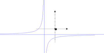
Figure 2. The real part of the hyperbola defined by $f$.

The amoeba and the coamoeba of the curve with defining polynomial $f(z,w)=1+\tau z+\tau w+zw$ with $0<\tau<1$ is given as in Figs. 3 and 4, respectively.

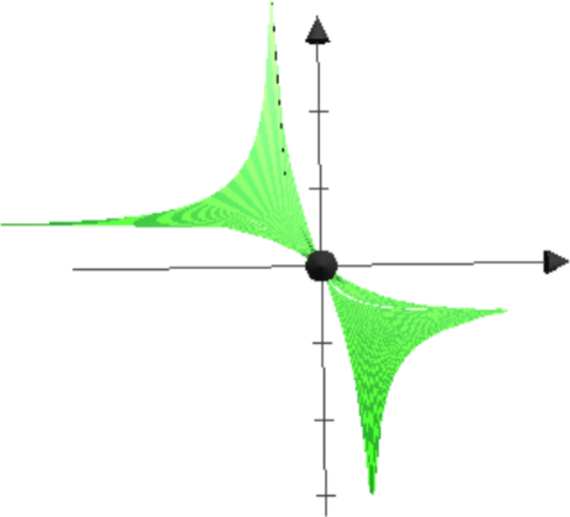
(a)

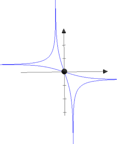
(b)

Figure 3. (A) Complex amoeba of the hyperbola defined by $f$. (B) Image under the logarithmic map of the real part of the hyperbola defined by $f$.

Figure 4. Coamoeba of the curve $\mathcal{C}$ with defining polynomial $f(z,w)=1+\tau z+\tau w+zw$ with $0<\tau<1$ in the fundamental domain $[0,2\pi]\times[0,2\pi]$ of the real torus $\mathop{\rm Log}\nolimits^{-1}(\mathcal{O})=(S^{1})^{2}$. The intersection of the curve $\mathcal{C}$ with $\mathop{\rm Log}\nolimits^{-1}(\mathcal{O})$ is the union of the two arcs which is a topological circle.

∎

Example 3.7.

Here are some examples of knots in the coamoebas of a complex algebraic plane curves.

(a) $f(z,w)=1+\tau z^{2}w^{2}+\tau z^{2}w^{3}+z^{4}w^{5}$.

(b) $f(z,w)=1+\tau z^{3}w^{3}+\tau zw^{2}+z^{4}w^{5}$.

Figure 5. Coamoebas with defining polynomials $f(z,w)$, with $0<\tau<1$.

Corollary 3.8.

Let $f_{(p,q)}$ be the polynomial defined as follows:

$$f_{(p,q)}(z,w)=1+\tau z^{p}+\tau w^{q}+\tau z^{p}w^{q}$$

where $\tau$ is a strictly positive real number such that $\tau\neq 1$, $p$ and $q$ are positive integer numbers with $(p,q)=c$. Then, the amoeba of the curve $V_{f_{(p,q)}}$ with defining polynomial $f_{(p,q)}$ contains the origin $\mathcal{O}\in\mathbb{R}^{2}$, and the inverse image of the origin with the logarithmic map is as follows:

• If $(p,q)=1$ (i.e. $p$ and $q$ are coprime), then $\mathop{\rm Log}\nolimits^{-1}(\mathcal{O})$ is a $(p,q)$-torus knot.

• if $(p,q)=c\neq 1$, then $\mathop{\rm Log}\nolimits^{-1}(\mathcal{O})$ is a $(p,q)$-torus link with $c$ connected components.

Proof.

The coamoeba when $p=q=1$ is given in Figure 4. Using Lemma 2.7, and the fact that $f_{(p,q)}=f_{D}$ where $D$ is the diagonal matrix with coefficients $p$ and $q$ the result follows immediately. ∎

Example 3.9.

Here some other examples of some known knots as a critical values of argument map restricted to a complex algebraic plane curves i.e. the contour of their coamoebas.

(a) $0<\tau<1$.

(b) $\tau>1$.

Figure 6. Coamoeba of the curve with defining polynomial $f(z,w)=1+\tau z^{2}+\tau w^{2}+z^{2}w^{2}$ with (A) $0<\tau<1$ and (B) $\tau>1$.

Figure 7. Hopf link.

(a) $0<\tau<1$.

(b) $\tau>1$.

Figure 8. Coamoeba of the curve with defining polynomial $f(z,w)=1+\tau z^{3}+\tau w^{3}+z^{3}w^{3}$ with (A) $0<\tau<1$ and (B) $\tau>1$. the union of the one-dimensional connected components of the critical values of the argument map is precisely the co-called Borromean rings.

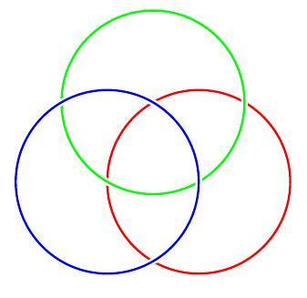
Figure 9. Borromean rings

(a) $0<\tau<1$.

(b) $\tau>1$.

Figure 10. Coamoeba of the curve with defining polynomial $f(z,w)=1+\tau z^{2}+\tau w^{3}+z^{2}w^{3}$ with (A) $0<\tau<1$ and (B) $\tau>1$ (Trefoil knots).

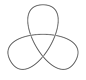
(a)

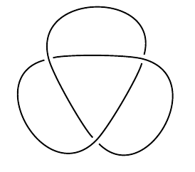
(b)

Figure 11. Trefoil knots

4. (Co)Amoebas and singularities of complex hypersurfaces

In this section we start by recalling some useful notions and known results that we need. Let $f$ be a non-constant holomorphic function defined on an open subset $U\subset\mathbb{C}^{n+1}$ containing the origin with $f(0)=0$, and such that the Jacobian $[\frac{\partial f}{\partial z_{0}}\cdots\frac{\partial f}{\partial z_{n}}]$ of $f$ has rank zero at the origin. This means that the origin is a critical point of $f$. In other words, the origin is a singularity of the fiber $V=f^{-1}(0)$. If $U$ is sufficiently small, then $0\in\mathbb{C}$ is an isolated critical value of $f$, and the fibers of $f$ over $\mathbb{C}\setminus\{0\}$ are nonsingular. If $f$ is a polynomial, then Milnor proved the following:

Theorem 4.1.

Let $f$ be a polynomial as above. Then, for any $\varepsilon>0$ sufficiently small, there exists a small $\delta>0$ such that:

$$f:B_{\varepsilon}\cap f^{-1}(D_{\delta}^{*})\longrightarrow D_{\delta}^{*}$$

is a smooth fiber bundle where $B_{\varepsilon}\subset\mathbb{C}^{n+1}$ is the open bull centered at the origin and of radius $\varepsilon$, and $D_{\delta}^{*}$ the punctured disk centered at the origin and of radius $\delta$. Moreover, the fiber diffeomorphism type of this fiber bundle is independent of the choice made.

Let $V\subset(\mathbb{C})^{n+1}$ be an algebraic hypersurface with defining polynomial $f$ such that $f(0)=0$. Moreover, suppose that $V$ has an isolated singularity at $0$. Let $S^{2n+1}$ be a sufficiently small sphere with center the point $p$. The intersection $V\cap S^{2n+1}$ is a $(2n-1)-$manifold $\mathcal{K}\subset S^{2n+1}$ called the link of the singularity. Let

$$\begin{array}[]{ccccl}\phi&:&S^{2n+1}\setminus\mathcal{K}&\longrightarrow&S^{1}\\ &&z&\longmapsto&\displaystyle\frac{f(z)}{|f(z)|}.\end{array}$$

By Milnor (see [Mil-68]) $\phi$ is a fibration and $\mathcal{K}$ is a fibred knot. When $n=1$, the knot $\mathcal{K}\subset S^{3}$ is well known. A necessary and sufficient condition that a $\mathcal{K}\subset S^{3}$ occur as the link of a singularity of an algebraic curve it to be a compound torus link with some other conditions.

Example 4.2.

Let $\mathcal{C}\subset\mathbb{C}^{2}$ be a complex plane curve such that the point $(0.0)$ is an isolated singularity of $\mathcal{C}$. Let $S^{3}_{\varepsilon}=\{(z,w)\in\mathbb{C}^{2}\,\Big{|}\,|z|^{2}+|w|^{2}=\varepsilon^{2}\}$, and let $\mathcal{K}=\mathcal{C}\cap S_{\varepsilon}$. By Milnor’s Theorem, $\mathcal{K}$ is the union of disjoint loops. Let $p\notin\mathcal{K}$ and $\pi:S_{\varepsilon}\setminus\{p\}\longrightarrow\mathbb{R}^{3}$ be the stereographic projection. Then the image of $\mathcal{K}$ under the projection $\pi$ is a link called the link of the singularity. For example the link of the singularity of the curve $w^{2}-z^{3}=0$ is the trefoil knot. More generally, In 1928, Brauner proved that for the curve $z^{p}+w^{q}=0$, $\mathcal{K}$ is a torus link $T_{(p,q)}$, which is a knot if $p$ and $q$ are co-prime. This fact will be proved in the next theorem using the theory of (co)amoebas.

Let $\mathcal{C}$ be the complex plane curve with defining polynomial $f(z,w)=z^{p}-w^{q}$. Let $\varepsilon$ be a small positive number. There exist small positive real numbers $\xi$ and $\eta$ such that the 3-dimensional sphere $S^{3}_{\varepsilon}\subset\mathbb{C}^{2}$ centered at the origin and with radius $\varepsilon$ is homeomorphic to the union of two solid tori glued along their boundaries the real 2-dimensional torus. In other words,

$$S^{3}_{\varepsilon}=D_{\xi}\times S^{1}_{\eta}\cup_{S^{1}_{\xi}\times S^{1}_{\eta}}S^{1}_{\xi}\times D_{\eta},$$

where $D_{\xi}\subset\mathbb{C}$ (resp. $D_{\xi}\subset\mathbb{C}$) is a closed 2-dimensional disc centered at the origin and with radius $\xi$ (resp. $\eta$), where $\xi^{2}+\eta^{2}=\varepsilon^{2}$, and $\xi^{p}=\eta^{q}$. Let Arg be the argument map coordinate wise, and let’s denote by $co\mathscr{A}_{\mathcal{C}}$ the coamoeba of the curve $\mathcal{C}$. In fact, $(z,w)\in S^{3}_{\varepsilon}\cap\mathcal{C}$ if and only if $|z|^{2}+|w|^{2}=\varepsilon^{2}$, and $z^{p}=w^{q}$. Thus, if $0<\xi$ is a small positive number, $|z|=\xi$, and $|w|=\eta=\xi^{\frac{p}{q}}$. Choose $\varepsilon$ such that $\xi^{2}+\eta^{2}=\varepsilon^{2}$.

$$\begin{array}[]{ccccccl}\textrm{Arg}&:&S^{3}_{\varepsilon}\cap\mathcal{C}&\hookrightarrow&S^{1}_{\xi}\times S^{1}_{\eta}&\longrightarrow&co\mathscr{A}_{\mathcal{C}}\subset S^{1}\times S^{1}\\ &&(z,w)&\longmapsto&\displaystyle(z,w)&\longmapsto&\displaystyle\Big{(}\frac{1}{\xi}z,\frac{1}{\eta}w\Big{)}.\end{array}$$

Theorem 4.3.

Let $\mathcal{C}\subset\mathbb{C}^{2}$ be the complex plane curve with defining polynomial $f(z,w)=z^{p}-w^{q}$. The polynomial $f$ is such that $f(0,0)=0$ and it has an isolated singularity at the point $(0,0)$. Then the link of this singularity is equal to the coamoeba of $\mathcal{C}$ which is the torus link $T_{(p,q)}$ (this is a knot if $p$ and $q$ are co-prime).

Proof.

We show Theorem 4.3 by reviewing Example 4.2. Consider the polynomial $f(z,w)=w^{2}-z^{3}$, which has an isolated singularity at the point $(0,0)$ called cusp. The solutions of the equation $f(z,w)=0$ are given as follows. First, let $w=tz^{\mu}$ with $t\in\mathbb{C}^{*}$ and where in this example $\displaystyle\mu=\frac{3}{2}$. In other words, if $\displaystyle w=tz^{\frac{3}{2}}$, then

$$f(z,w)=f(z,tz^{\frac{3}{2}})=z^{3}(t^{2}-1).$$

As we are working in the complex algebraic torus, $f(z,tz^{\frac{3}{2}})=0$ if and only if $t=\pm 1$, which means that we have tow solutions $w_{1}=z^{\frac{3}{2}}$ and $w_{2}=-z^{\frac{3}{2}}$. The graph of the set of arguments corresponding to the first solution in the 2-dimensional torus $S^{1}\times S^{1}$ is the one given by the segment in the fundamental domain $[0,2\pi]\times[0,2\pi]$:

$$\arg(w)=\frac{3}{2}\arg(z).$$

Also, the graph of the set of arguments corresponding to the second solution in the 2-dimensional torus $S^{1}\times S^{1}$ is the one given by the segment

$$\arg(w)=\pi+\frac{3}{2}\arg(z),$$

where $-1=e^{i\pi}$, and then its argument is $\pi$. We glue the graph of the two solutions and we take the set of all arguments in the 2-dimensional torus $S^{1}\times S^{1}$ to get a knot, which is the trefoil.

This knot is precisely the coamoeba of the intersection of the zero locus of $f$ and the a small sphere centered at the point $(0,0)$.

Figure 12. The green line is the graph of the first solution $w_{1}$, and the red line is the graph of the second solution $w_{2}$, and their union is a knot called the trefoil. The square represents the fundamental domain $[0,2\pi]\times[0,2\pi]$ of $S^{1}\times S^{1}$.

In general, if $f(z,w)=z^{p}-w^{q}$, then $\displaystyle\mu=\frac{p}{q}$ and $w=tz^{\frac{p}{q}}$ is a solution of the equation $f(z,w)=(1-t^{q})z^{p}=0$. Thus, $t=e^{\frac{2i\pi k}{q}}$, with $k=0,1,\ldots,q-1$. We follow the method used above in the particular case of $p=3$ and $q=2$ to obtain a similar result. Two cases should be distinguished, the case where $(p,q)=1$ (i.e. co-prime), and the case where $(p,q)=c\neq\pm 1$. If $(p,q)=1$, we obtain only one connected component i.e a knot which is the coamoeba of the plane curve defined by $f$. In fact,

$$\arg(w)=\frac{2\pi k}{q}+\frac{p}{q}\arg(z),\quad\quad\textrm{with}\,\,\,k=0,\ldots,q-1,$$

where $w=|w|e^{i\arg w}$,  $z=|z|e^{i\arg z}$  and $\displaystyle 0\leq\frac{p}{q}\arg(z)\leq 2\pi$. This provides us a circle in the real torus which is a $(p,q)-$torus knot. If $(p,q)=c\neq\pm 1$, then we obtain $\textrm{intl}_{\mathbb{Z}}\Big{(}[(p,0),(0,q)]\Big{)}=c$ connected components i.e. a link, which is, as before, the coamoeba of the plane curve defined by $f$, where each connected component corresponds to a branch passing trough the singularity. ∎

Generally, let $f$ be a polynomial of the following form:

$$f(z,w)=\sum_{i+\mu j=c}a_{ij}z^{i}w^{j},$$

where $\mu$ is a rational number equal to $\displaystyle\frac{p}{q}$, the pair $(i,j)\in(\mathbb{Z}_{\geq 0})^{2}$, and $c\in\mathbb{Q}$ is a constant. In this case, the polynomial is said to be quasi-homogeneous. In other words, all the powers are contained in a line of slope $\displaystyle-\frac{1}{\mu}$ and we obtain a solution of the form $w=tz^{\mu}$ for the equation $f(z,w)=0$. After substitution of this solution in the expression of $f$ we get the following:

$$f(z,tz^{\mu})=\sum_{i+\mu j=c}a_{ij}z^{i}z^{\mu j}t^{j}=\sum_{i+\mu j=c}a_{ij}z^{c}t^{j}=z^{c}\sum_{i+\mu j=c}a_{ij}t^{j}.$$

We get an univariate polynomial $h(t)=\sum_{i+\mu j=c}a_{ij}t^{j}$. In general, one can write $f$ as a sum of a quasi-homogeneous polynomial $g$, and a second polynomial consisting of higher order terms. Then one can obtain the solution to the quasi-homogeneous part as before, and we can say that this is an approximate solution to the equation $f=0$.

Example 4.4.

Let $\mathcal{C}\subset\mathbb{C}^{2}$ be the complex algebraic curve with defining polynomial $f(z,w)=w^{2}+z^{3}w-2z^{6}$. The curve $\mathcal{C}$ has an isolated singularity at the point $(0,0)$, with $f(0,0)=0$. Clearly the polynomial $f$ is quasi-homogeneous, and the powers of its monomials lie on a straight line with slope $\displaystyle-\frac{1}{3}$. So, with the notation used above $\mu=3$. Thus, by setting $w(t)=tz^{3}$, we get a solution of $f(z,w)=0$. In fact, $f(z,tz^{3})=(t^{2}+t-2)z^{6}=0$ when $t=1$, or $t=-2$. Hence, we obtain two solutions $w_{1}=z^{3}$ and $w_{2}=-2z^{3}$. The link of this singularity has two connected components where each component is an unknotted circle and equal to the coamoeba of these two solutions (see Figure ??).

Figure 13. The blue line is the graph of the first solution $w_{1}$ which in an unknotted circle. The red line is the graph of the second solution $w_{2}$, which is also an unknotted circle. Their union is a linked two circles called Hopf link. The square represents the fundamental domain $[0,2\pi]\times[0,2\pi]\subset\mathbb{R}^{2}$ universal covering of $S^{1}\times S^{1}.$

Figure 14. Hopf link.

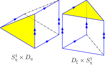
Figure 15. Left: The solid torus $S^{1}_{\xi}\times D_{\eta}\subset\mathbb{C}\times\mathbb{C}$ where $D_{\eta}$ is the 2-dimensional disc contained in $\mathbb{C}$ (the second factor) centered at the origin and with radius $\eta$. Right: The solid torus $D_{\xi}\times S^{1}_{\eta}\subset\mathbb{C}\times\mathbb{C}$ where $D_{\xi}$ is the 2-dimensional disc contained in $\mathbb{C}$ (the first factor) centered at the origin and with radius $\xi$.

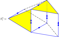
Figure 16. The 3-dimensional sphere as the gluing of two solid tori.

Example 4.5.

Consider the polynomial $f(z,w)=z^{5}-w^{2}$, which has an isolated singularity at the point $(0,0)$ called cusp. The solutions of the equation $f(z,w)=0$ are given as follows. First, let $w=tz^{\mu}$ with $t\in\mathbb{C}^{*}$ and where in this case $\displaystyle\mu=\frac{5}{2}$. In other words, if $\displaystyle w=tz^{\frac{5}{2}}$, then

$$f(z,w)=f(z,tz^{\frac{5}{2}})=z^{5}(1-t^{5}).$$

Therefore, $f(z,w)=0$ has five solutions $\displaystyle w=e^{\frac{2i\pi k}{5}}z^{\frac{5}{2}}$ with $k=0,1,2,3,4$. The graph of the set of arguments corresponding to the five solutions in the 2-dimensional torus $S^{1}\times S^{1}$ are given by the segments in the fundamental domain $[0,2\pi]\times[0,2\pi]$:

$$\arg(w)=\frac{2\pi k}{5}+\frac{5}{2}\arg(z),\quad\quad k=0,1,2,3,4.$$

where $\displaystyle 0\leq\frac{5}{2}\arg(z)\leq 2\pi$, in other words, $\displaystyle 0\leq\arg(z)\leq\frac{4}{5}\pi$. We glue the graphs of the five solutions and we take the set of all arguments in the 2-dimensional torus $S^{1}\times S^{1}$ to obtain a knot, which is the cinquefoil. This knot is precisely the coamoeba of the intersection of the zero locus of $f$ and the a small sphere centered at the point $(0,0)$.

Figure 17. The five segments with five different colors are the graphs of the five solutions. The gluing of these graphs produces the cinquefoil knot. The square represents the fundamental domain $[0,2\pi]\times[0,2\pi]\subset\mathbb{R}^{2}$ universal covering of $S^{1}\times S^{1}.$

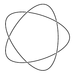
Figure 18. The cinquefoil. $z^{5}-w^{2}=0$

References

[CMNL-23]A. Chatterjee, T. S. Mahesh, M. Nisse, and Y.-K. Lim,Observing Algebraic Variety of Lee-Yang Zeros in Inaccessible Systemsin preparation
[FHKV-05]B. Feng, Y. He, K. D. Kennaway
and C. Vafa, Dimer models from mirror symmetry and quivering amoeba,
Adv. Theor. Math. Phys. 12, n 3 (2008), 489-545.
[FPT-00]M. Forsberg, M. Passare
and A. Tsikh, Laurent determinants and arrangements of hyperplane amoebas,
Advances in Math. 151, (2000), 45-70.
[GKZ-94]I. M. Gelfand, M.
M. Kapranov and A. V. Zelevinski, Discriminants, resultants and
multidimensional determinants,
Birkhäuser Boston 1994.
[IMS-07]I. Itenberg, G. Mikhalkin and E. Shustin, Tropical Algebraic Geometry,
Oberwolfach Seminars, Volume 35,
Birkhäuser Basel-Boston-Berlin 2007.
[K-00]M. M. Kapranov, Amoebas over
non-Archimedean fields, Preprint 2000.
[LN-21]Y.-K. Lim and M. Nisse, The zero-temperature limit of grand canonical ensembles via tropical geometry, Anal. Math. Phys. 11 (2021) 113.
[LY-52a]C. N. Yang and T. D. Lee,
Statistical theory of equations of state and phase transitions. 1. Theory of condensation,
Phys. Rev. 87 (1952), 404-409.
[LY-52b]T. D. Lee and C. N. Yang,
Statistical theory of equations of state and phase transitions. 2. Lattice gas and Ising model,
Phys. Rev. 87 (1952), 410-419.
[LN-23]Y.-K. Lim and M. Nisse, (Co)Amoebas and links of singularities, in preparation.
[MS-09]Diane Maclagan and Bernd Sturmfels, Introduction to Tropical Geometry, Grad. Stud. Math., vol. 161, American Math. Soc., 2015.
[M1-02]G. Mikhalkin , Real algebraic
curves, moment map and amoebas, Ann. of Math. 151 (2000), 309-326.
[M2-04]G. Mikhalkin, Enumerative Tropical
Algebraic Geometry In , J. Amer. Math. Soc. 18, (2005), 313-377.
[Mil-68]J. Milnor, Singular Points of Complex Hypersurfaces, Princeton, New Jersey: Princeton University Press and the University of Tokyo Press, 1968.
[N1-09]M. Nisse, Geometric and Combinatorial Structure of Hypersurface Coamoebas, Preprint https://arxiv.org/pdf/0906.2729.pdf
[N2-09]M. Nisse, Amoebas and Coamoebas Relationships and Similarities, 1047th AMS Meeting, University of Illinois, Urbana-Champaign, March 27-29, p 94, (2009)..
[NS1-13]M. Nisse and F. Sottile, Non-Archimedean coAmoebas, Contemporary Mathematics
Amer. Math. Soc. Vol. 605, (2013), 73–91.
[NS2-13]M. Nisse and F. Sottile, The Phase Limit Set of a Variety, Algebra &
Number Theory 7(2) (2013) 339–352,
[PR1-04]M. Passare and H.
Rullgård, Amoebas, Monge-Ampère measures, and triangulations
of the Newton polytope, Duke Math. J. 121, (2004), 481-507.
[PT-05]M. Passare and A. Tsikh, Amoebas: their spines and their contours, Contemporary Mathematics 377 (2005) 275–288.
[RST-05]J. Richter-Gebert, B. Sturmfels et T. Theobald ,
First steps in tropical geometry, Idempotent mathematics and mathematical physics,
Contemp. Math., 377, (2005), 289-317 , Amer. Math. Soc., Providence, RI, 2005.
[R-01]H. Rullgård, Polynomial amoebas and convexity, Research Reports In Mathematics Number 8,2001, Department Of Mathematics Stockholm University.