Few-shot Multispectral Segmentation with Representations Generated by Reinforcement Learning

Abstract

The task of multispectral image segmentation (segmentation of images with numerous channels/bands, each capturing a specific range of wavelengths of electromagnetic radiation) has been previously explored in contexts with large amounts of labeled data. However, these models tend not to generalize well to datasets of smaller size. In this paper, we propose a novel approach for improving few-shot segmentation performance on multispectral images using reinforcement learning to generate representations. These representations are generated in the form of mathematical expressions between channels and are tailored to the specific class being segmented. Our methodology involves training an agent to identify the most informative expressions, updating the dataset using these expressions, and then using the updated dataset to perform segmentation. Due to the limited length of the expressions, the model receives useful representations without any added risk of overfitting. We evaluate the effectiveness of our approach on several multispectral datasets and demonstrate its effectiveness in boosting the performance of segmentation algorithms.

1 Introduction

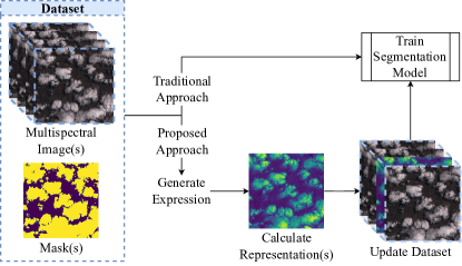
Figure 1: A one-shot example of the proposed approach. Our system works by using the dataset to generate a mathematical expression, which is thereby used to update the dataset, resulting in a performance improvement compared to the direct approach when trained for segmentation.

Multispectral imagery is a powerful tool in a variety of applications in domains such as remote sensing, medical imaging, and thermal imaging. The inherent ability of multispectral images to capture data across various wavelengths of light provides a wealth of information about the dynamics of the surface being captured. A fundamental task in harnessing this data is image segmentation, which involves identifying distinct regions or objects based on certain criteria. However, existing work relies on large datasets to achieve significant performance. The core challenge of working with smaller datasets is generalizing to a wider population.

To address this task, spectral indices have been widely employed ([31, 28, 22]) as a generalized representation of a class of interest. These indices are mathematical expressions between bands of a multispectral image, designed to create representations based on the underlying reflective properties of the object of interest. For instance, the Normalized Difference Vegetation Index (NDVI) is commonly used to assess vegetation health, while the Normalized Difference Water Index (NDWI) is employed for water body detection.

However, the utility of spectral indices is constrained by their availability and adaptability to different contexts. Typically, these indices are designed for a limited set of predefined classes, making them less effective when applied to novel or specialized tasks. Furthermore, the process of creating custom indices tailored to specific segmentation objectives is often a laborious and iterative trial-and-error procedure that demands substantial domain expertise.

In this paper, we propose a novel approach for improving segmentation performance on multispectral images as demonstrated by Figure 1. Our system begins by discovering a mathematical expression (in other words, a spectral index) that is expected to yield a good segmentation performance. We accomplish this using a reinforcement learning formulation by using Monte Carlo Tree Search (MCTS) [5] to explore possible expressions/indices, training a Generative Pretrained Transformer-based model [29, 24] as the policy network to generate expressions with higher rewards, and then re-running MCTS with the improved model to facilitate better exploration. After identifying a suitable mathematical expression, we evaluate the expression on each image and integrate the resulting channel with the rest of the channels of the image.

The reasoning behind the hypothesis that spectral indices would help improve segmentation performance is that certain mathematical functions are difficult for neural networks to represent. For example, a simple multiplication between two channels would require a significant number of neurons to be accurate over a wide range of inputs. By using spectral indices as input features, we can provide the neural network with more informative and relevant input data, improving its ability to learn and generalize to new examples. Empirically, the initial hypothesis holds.

Accordingly, the contributions of our research are as follows:

• We propose a novel application of reinforcement learning for discovering spectral indices that improve few-shot segmentation performance in multispectral images.

• We address the challenging task of few-shot multispectral segmentation which, to the best of our knowledge, has not been previously explored in the literature.

• We demonstrate the effectiveness of our proposed approach on several datasets by comparing the performance against several baseline methods.

2 Background and Related Work

Spectral indices for segmentation

Spectral indices have been used to assist segmentation in a variety of techniques. Traditional methods directly use algorithms such as Otsu’s thresholding [21] or watershed algorithms [16] to binary segment the single channel result of evaluating spectral indices [22, 23, 31]. However, these techniques are only viable when there already exist spectral indices tailored to the classes of interest.

Our work draws inspiration from MSNet [28] which utilizes spectral indices for the segmentation of arbitrary classes. They demonstrate the benefits of incorporating the Normalized Difference Vegetation Index (NDVI) and the Normalized Difference Water Index (NDWI) as additional channels of multispectral images for segmentation. This suggests that these indices carry some information that is not easily represented by deep learning models.

RL for expression induction and theorem proving

The tasks of expression induction and theorem proving follow a formulation similar to that of index generation as explored in this paper. One early instance of these tasks is found in [30] where an RL agent is employed to generate symbolic expressions, specifically polynomial expressions. In this setup, an agent, implemented as a Recurrent Neural Network (RNN), iteratively selects symbols that collectively form an expression in post-order notation. Building upon a similar foundation, [19] adopts an analogous strategy to leverage RL to estimate the policy function of an RL agent, with the dimensions of the state serving as the operands of the mathematical expression. RL-based agents have also been used to navigate tableaux trees (trees with branches representing sub-formulae of theorems) for proving first-order logic [17, 9]. The representation of the state in our methodology contrasts with that of these techniques.

As opposed to using a tree-based representation with post-order traversal, we use the expression symbols under in-order traversal to represent the state. This makes each state directly human-readable, resulting in an improved explainability of a given state while enabling the formulation of the agent’s task as a text generation task.

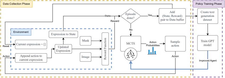
Figure 2: Index Generator Training Process. Each training iteration of the index generator has 2 main phases: the data collection phase and the policy training phase. Expression samples are generated during the data collection phase by a generative model that guides MCTS. The model is improved by using the generated samples to train the policy network during the policy training phase.

Monte Carlo Tree Search (MCTS)

MCTS [5] is an algorithm that uses simulations to determine the best action to be taken from a given state. The simulation is done iteratively where each iteration consists of selecting an action, expanding a branch on a tree for the selected action, followed by the simulation from a leaf node on the tree. The exploration-exploitation trade-off is managed by a measure (often the Upper Confidence Bound (UCB1) score [3]) which prioritizes nodes that have a low visitation count but have yielded high returns after simulation. While the vanilla MCTS algorithm takes random actions during simulation, later approaches [26, 2, 27, 11] use a neural network to guide the simulation. These algorithms are broadly known as Neural MCTS.

Our proposed methodology builds on these concepts by using a GPT-based network as the policy network to guide the simulation in identifying an effective spectral index for a given segmentation task.

Few-shot Segmentation

Few-shot segmentation is the task of segmenting objects using a small amount of labeled data. Most existing work approaches this task by comparing the unlabeled image (query image) against the labeled image (support image) at inference time [4]. However, some work uses techniques such as data augmentation [33, 7, 8] and sample synthesis [1, 32], either as standalone techniques or for boosting the performance of existing techniques.

In contrast to these approaches, our research focuses on identifying an expression that extracts the most useful and representative features using a limited amount of data.

3 Methodology

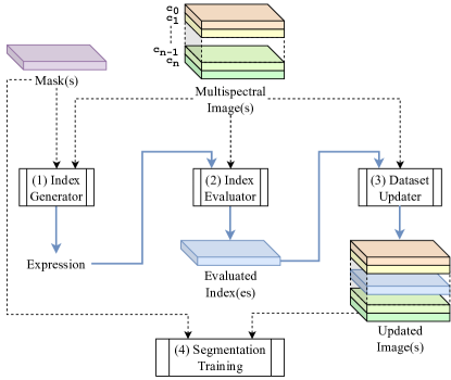
Figure 3: The proposed methodology and its 4 main components. (1) Index Generator: Uses the train set (image-mask pairs) to generate an expression. (2) Index Evaluator: Uses the generated expression and the original images to create the evaluated indices. (3) Dataset Updater: Uses the evaluated indices to update the original images. (4) Segmentation Trainer: Trains a segmentation model using the updated images. Note that the Index Evaluator, the Dataset Updater, and the Segmentation Trainer are also used within the Index Generator as described in Section 3.1.

Figure 3 presents the proposed methodology consisting of four main components: (1) Index Generator, (2) Index Evaluator, (3) Dataset Updater, and (4) Segmentation Training. The index generator generates a mathematical expression which is then used to produce the evaluated indices. The evaluated indices are integrated with the dataset using the dataset updater, and the updated dataset is used for training. In the sections that follow, we discuss the first 3 components. The place of the segmentation trainer can be taken by any multispectral segmentation approach.

3.1 Index Generator

In this section, we begin by describing the formulation of the RL problem. Next, we will discuss the training process of the agent. Finally, we will discuss several implementation adaptations we made to facilitate the task.

3.1.1 RL Formulation.

Formulating the problem of spectral index generation as a reinforcement learning task can be done by defining the state space, action space, environment, and reward function.

States and Actions.

The state is defined by the currently generated portion of the mathematical expression while the actions are represented by the symbols that form the expression. Additionally, a terminal state is defined by the presence of the ”=” symbol at the end of the expression. Accordingly, the action space consists of the following symbols:

• Expression symbols: (, ), +, -, *, /, square, square root (8 symbols)

• Image Channels: $c_{0}$, $c_{1}$, … , $C_{n\_channels}$ (n_channels symbols)

• End symbol: $=$ (1 symbol)

The maximum length of the expression/state is a hyperparameter that can be adjusted based on the context or domain (longer expressions create more complex representations).

Environment.

The environment’s purpose is to provide the next state and reward when taking an action from the current state. Here, the newly generated action/symbol is appended to the current expression and given as the output state, while the reward is calculated via the reward function.

Reward - MCTS.

The reward for guiding MCTS is defined for 3 different cases as follows.

$$R(s)=\begin{cases}-1,&\text{if episode ended at an invalid state}\\ r(s),&\text{if episode ended at a valid state}\\ 0,&\text{otherwise (episode has not ended)}\\ \end{cases}$$ (1)

Here, the function $r(s)$ is a function that approximates how good the given state/expression $s$ is for the segmentation performance.

In addition to the expression, the reward function shall also use the existing labeled images to calculate the reward. An evaluated index will be calculated for each image of the training set as per Section 3.2, which can thereby be used to calculate the reward. Each evaluated index is a single-channel image with the same height and width as the original image.

As part of this research, we evaluate several different reward functions for r(s) that follow the same base structure shown below:

$$score =f(I_{e},M)$$ (2)

$$score^{\prime} =f(1-I_{e},M)$$ (3)

$$r(s) =min(score,score^{\prime})$$ (4)

where $I_{e}\in\mathbb{R}^{H\times W}$ refers to an evaluated index that has been standardized, clipped, and scaled to a $[0,1]$ range, $M\in\mathbb{R}^{H\times W}$ refers to the ground truth segmentation mask corresponding to the image from which $I_{e}$ is produced, and $f(I_{e},M)$ refers to the heuristic function for estimating the utility of using $I_{e}$ to predict $M$. Note that the final score for a given expression is the average of $r(s)$ over all or a subset of images (in cases with a large dataset).

The intuition behind the use of the minimum of $score$ and $score^{\prime}$ is that $1-I_{e}$ is a simple operation for any network, given $I_{e}$, and either of the two may be the default representation being used within the network, based on the initialization of weights. Obtaining the minimum of the 2 scores penalizes the lack of information in either of the representations, resulting in the expression that leads to the highest similarity to the mask in most cases to be selected.

The evaluated functions for the choice of $f$ in 2 - 4 include:

1. F1 Score (with a threshold for $I_{e}$ of 0.5 to get a binary mask

2. Area Under the Curve (AUC) (with threshold, similar to the F1 score)

3. Cosine Similarity (CS)

4. Intersection over Union (IoU)

5. Pearson Correlation Coefficient (PCC)

Reward - Training

Once an expression is generated, we calculate the actual segmentation performance of the expression by training a model using only the evaluated indices. Since the completion of an expression occurs much less frequently than in MCTS, this is a practical way to obtain a more accurate score for the performance gained from the expression.

3.1.2 RL Training Process

The training process requires a set of multispectral images with segmentation masks (tensors with ones in the areas of interest and zeros elsewhere) for each image as input.

As shown in Figure 2, each iteration of the training process is performed in two phases: (1) Data Collection and (2) Policy training.

Data Collection Phase.

Each iteration uses MCTS to generate a probability distribution over the actions based on the simulated return observed for each action. This probability distribution is then used to sample the next action to be taken by the environment. If the action results in the termination of the episode (in other words, if the last action is the “=” symbol), then the expression and its training reward (Section 3.1.1) are passed into the data buffer. Otherwise, the state is passed into MCTS for simulation. Each iteration of the data collection phase generates several expressions. The number of generated expressions is a tunable hyperparameter.

After their generation, the generated expressions are stored in a data buffer. Of the stored expressions, the expressions that yielded a high reward are passed to training. The criteria for classifying an expression as ”high-reward” is discussed in the Adaptive Data Buffer. section.

While one image and its mask are sufficient to execute the data collection phase, the result is likely to be more generally beneficial if the average of more images is used to calculate the reward. Thus, there is a configurable trade-off between the lower execution time and the discovery of the better-performing expression.

Policy Training Phase.

In the policy training phase, the GPT-based model (policy network) is trained to generate useful expressions. In other words, given the current state, we train the model to generate the next symbol. With each iteration, the model learns to generate better-performing expressions. Subsequently, the MCTS exploration improves. This is because MCTS only explores a limited number of branches and the exploration thereafter is simulated using the symbols generated by the model. A better-performing policy network can explore higher-reward expressions without the guidance of MCTS.

3.1.3 Implementation Adaptations

Pretraining for valid output generation.

Each iteration of MCTS spends a non-negligible amount of time evaluating the expression. Since the expression validity can be evaluated with a $(1,1,n_{c}hannels)$-shaped tensor, the expression evaluation time can be significantly reduced during the pretraining stage. As a result, the model can learn to generate valid expressions much faster. This also gives the added benefit of providing a pretrained model to initialize weights for a new task, assuming the new task works with the same number of channels.

During the pretraining phase, certain tendencies are observed in the behavior of the agent. Firstly, the agent often generates short expressions. This may be because the more complex the expression, the easier it is to deviate from a regular range of values. Secondly, the agent tends to avoid opening parentheses. This is likely caused by the fact that once an opening parenthesis is generated, the expression remains invalid until a closing parenthesis is generated and this leads to a higher chance of negative rewards.

It is also observed that a significant fraction of existing remote-sensing indices is ”unitless”. In other words, if each channel of the multispectral image is given a unit of measurement, the spectral index resulting from a mathematical operation between those bands lacks a unit.

Accordingly, to motivate the agent to address the aforementioned considerations, the reward for pretraining $r(s)$ is defined as presented in equation 8.

$$r_{len} = 0.02\times l_{exp}$$ (5)

$$r_{par} = 0.2\times n_{par}$$ (6)

$$r_{unit} = \begin{cases}1,\text{if expression is unitless}\\ 0,\text{otherwise}\\ \end{cases}$$ (7)

$$r(s) = 0.5+r_{len}+r_{par}+r_{unit}$$ (8)

where $l_{exp}$ is the length of the expression and $n_{par}$ is the number of pairs of parentheses in the expression.

Action validity.

Previous Action	Valid Actions
$start,(,+,-,\times,/$	$(,channel$
$channel,)$	$+,-,\times,/,),=$

Table 1: The list of valid actions, given the previous action, where $start$ refers to the starting state (empty expression) and $channel$ refers to a channel of the image.

At each state, we define a set of valid actions based on the previous action as shown in Table 1. In addition, certain other checks are performed to avoid invalidity and redundancy where possible.

• The number of “)” symbols in the expression is always maintained to be less than or equal to the number of “(“ symbols in the expression. In other words, generating the “)” symbol is defined to be invalid if all opened parentheses have already been closed.

• Since enclosing a single symbol within parentheses is redundant as the parentheses can simply be removed, generating a closing parenthesis, two actions after generating an opening parenthesis, is defined to be an invalid action.

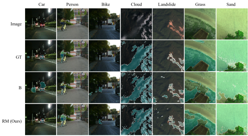
Figure 4: Qualitative Comparison between the baseline result (B) and Multi-index replacement (RM) across the datasets with the UNet model, along with the ground truth (GT).

Adaptive Data Buffer.

The classification of expressions as high-reward or low-reward can be achieved by various criteria. For the experiments performed in this research, this classification is performed by using an adaptive data buffer. The idea is to progressively reduce the size of the data buffer to get the GPT-based model to overfit to a set of expressions that provide a higher reward. We chose to implement this functionality as follows. The data collection phase is initially executed until the buffer reaches a certain capacity. The iterations that follow execute both the data collection phase and training phase. After each iteration, the buffer size is set to 95% of its current capacity, dropping the expressions within the 5% of lowest rewards. This is repeated until a certain minimum capacity is reached. This minimum capacity would be a relatively low number (e.g.: 20), such that the model may overfit to those expressions while also exploring expressions that contain similar symbols and structures.

3.2 Index Evaluator

The index evaluator uses the generated expression to create a single-channel image that we refer to as the evaluated index. This is obtained by performing pixel-wise operations across the channels based on the expression. For example, say the chosen expression is $c0\times c1=$. To evaluate this expression, for each image, we perform an element-wise multiplication between the pixels of the channel at index 0 and those at index 1.

3.3 Dataset Updater

We explore two main techniques by which the dataset can be updated using the evaluated index.

Concatenation

The first integration technique is to simply concatenate each evaluated index with their respective source images. So, given a 10-channel image, the concatenation would result in an 11-channel image. Additional expressions may also be evaluated and concatenated to include more representations.

Substitution

The second technique is to substitute a channel with an evaluated index. Here, it is important to consider which channels are being substituted as it may cause a loss of information. Accordingly, the evaluated index is only substituted with channels that appear within the expression.

Based on these techniques, we define 4 modes: Single-index concatenation (C), Multiple-index concatenation (CM), Single-index replacement (R), and Multiple-index replacement (RM). Each mode is empirically evaluated in Section 4.4. The best updating mode for a given dataset is determined by observing the validation accuracy of each mode.

Dataset	UNet [25]		DeepLabV3 [6]		UNet++ [34]
	Baseline	Ours	Baseline	Ours	Baseline	Ours
car	62.5	67.4 (RM)	55.4	58.2 (RM)	74.8	74.8 (CM)
person	46.4	48.4 (RM)	17.9	25.2 (RM)	47.3	48.5 (R)
bike	37.8	39.8 (RM)	31.1	53.5 (RM)	40.3	36.4 (R)
cloud	80.6	83.3 (RM)	62.0	65.6 (R)	82.3	84.2 (RM)
landslide	38.0	43.1 (RM)	18.7	20.5 (R)	35.9	42.8 (RM)
grass	58.0	73.6 (RM)	66.6	65.6 (R)	60.9	65.6 (RM)
sand	13.1	59.4 (RM)	12.6	41.3 (RM)	25.2	69.2 (RM)

Table 2: Overall Results. The table compares the IoU scores of the baseline model against that of the best dataset updating mode for each dataset class when trained on each model. (See Section 3.3)

Dataset	UNet [25]					DeepLabV3 [6]					UNet++ [34]
	B	C	CM	R	RM	B	C	CM	R	RM	B	C	CM	R	RM
car	62.5	63.0	61.1	65.0	67.4	55.4	58.1	58.9	58.0	58.2	74.8	72.0	74.8	60.6	71.2
person	46.4	41.8	47.0	45.1	48.4	17.9	19.0	16.8	22.0	25.2	47.3	51.2	53.5	48.5	45.1
bike	37.8	29.3	37.4	37.0	39.8	31.1	43.6	41.9	41.2	53.5	40.3	38.6	43.0	36.4	33.7
cloud	80.6	82.7	82.0	79.9	83.3	62.0	64.9	64.8	65.6	64.9	82.3	83.0	81.9	83.9	84.2
landslide	38.0	36.7	37.1	33.7	43.1	18.7	19.7	20.5	20.5	25.0	35.9	36.8	33.5	34.3	42.8
grass	58.0	61.7	63.3	73.6	73.6	66.6	62.3	63.7	65.6	61.9	60.9	61.7	60.4	70.2	65.6
sand	13.1	12.3	11.5	44.3	59.4	12.6	9.8	26.5	56.2	41.3	25.2	25.2	37.8	62.8	69.2

Table 3: Effects of Dataset Updating Mode. The table compares the IoU scores of the baseline model against each that of each updating mode. While RM can be thought of as a safe updating mode in most cases, it seems to be of more benefit to smaller models (UNet) in contrast to larger models (DeepLabV3 and UNet++).

4 Experiments

Datasets.

Due to the absence of previously created few-shot multispectral segmentation datasets, we explore the performance of the proposed approach across several multispectral datasets, MFNet [14], Sentinel-2 Cloud Mask Catalogue [12], Landslide4Sense [13], and RIT-18 [18]. For MFNet and RIT-18, which are multiclass segmentation datasets, we evaluate our approach on selected classes (car, person, and bike on MFNet; grass and sand on RIT-18). The datasets containing samples of each class are treated as individual datasets during experimentation. Accordingly, the final set of datasets consists of car, person, bike, cloud, landslide, grass, and sand.

To accommodate a few-shot context, we chose to randomly sample 50 data points from each dataset. These 50 data points are split into train, validation, and test in the frequencies of 20, 10, and 20, respectively.

4.1 Index Generation Experimental Details

Reward Heuristic Comparison.

As mentioned in Section 3.1.1, we evaluate the performance of several heuristic functions to estimate the segmentation performance for a given expression. To achieve this, we sample 200 randomly generated expressions as explored during the pretraining stage (Section 3.1.3). Each sampled expression is assigned a score by obtaining the actual segmentation performance (IoU) through training on the training sets of the MFNet datasets. Next, we calculate the heuristic scores for each of the expressions as defined by equation 4. Finally, we perform a correlation analysis between the scores of each heuristic function and the scores obtained through training, by calculating the t-statistic.

Function	Correlation	t-statistic	p-value
IoU	0.0554	0.7807	0.4359
CS	0.0599	0.8444	0.3995
F1	0.0667	0.9406	0.3481
AUC	0.0776	1.0952	0.2748
PCC	0.1417	2.0142	0.0453

Table 4: A statistical comparison of the correlations of each heuristic function with the training score

Based on the results presented in Table 4, it can be concluded that for the evaluated dataset, only the Pearson correlation shows a statistically significant correlation with the training performance at a significance level of 0.05. Thus, the PCC is used as the reward heuristic to evaluate each branch of the MCTS.

Index Selection.

The data buffer used in the RL algorithm contains the best-performing expressions at any given time. After allowing the RL algorithm to explore for a satisfactory amount of time, we choose the two best expressions for the segmentation experiments.

4.2 Segmentation Experimental Details

Training.

We evaluate the performance of the proposed approach on 3 segmentation model architectures, UNet [25], UNet++ [34], DeepLabV3 [6]. For each model, we use a ResNet50 model [15] pretrained on ImageNet [10] as the encoder. During training, all but the decoder of the model is frozen. We use the AdamW optimizer [20] with beta coefficients of 0.9 and 0.999, epsilon of 1e-8, and a weight decay of 1e-2. Each model is trained with learning rates of 1e-3 and 1e-4. The models undergo early stopping with 1000 epochs of patience by monitoring the validation loss. The trained models are then evaluated on the test set to obtain the final performances.

Evaluation Metrics.

We calculate the Intersection over Union (IoU), a.k.a. the Jaccard Index as given by equation 9.

$$IoU=\frac{TP}{TP+FP+FN}$$ (9)

where TP, FP, and FN denote the frequencies of true positives, false positives, and false negatives, respectively.

4.3 Overall Results

We compare the performance of the overall method against each baseline model and dataset (Table 2). While the proposed method results in a significant improvement in UNet, it can be observed that this advantage slightly decreases with increasing model size. We hypothesize that bigger models depend relatively less on the input representations.

We also perform a qualitative comparison between the baseline (B) model and the multi-index replacement (RM) mode (Figure 4). Through the comparison, we observe that the RM mode tends to be relatively less confused by objects that blend into the background in terms of color.

4.4 Ablation Studies

Effects of Index Minification.

We first perform a set of preliminary experiments to explore the impact of removing any components of the expression that are simple additions or subtractions of individual channels (Table 5). We refer to this alteration as index minification. For example, the expression for the car dataset ($(c_{2}-c_{0}-c_{1}-\sqrt{c_{1}})+c3=$) is compared against the minified expression ($\sqrt{c_{1}}=$). Similarly, the expression for the person dataset ($((c3/c2)*c0)-c3=$) is compared against its minified version ($(c3/c2)*c0=$). The objective is to test whether the inclusion of such trivial representations would not help improve segmentation performance since neural networks can easily learn them without the assistance of the index. While this decision seems to have a significant impact on performance, the direction of impact is observed to be split. On average, the smaller architecture (UNet) is observed to have better performance for the non-minified expression compared to the minified expression, and vice versa for the larger architecture (UNet++). This observation supports the intuition that the representations are better learned in the latter model.

Arch.	Dataset	C	CM	R	RM
UNet	Car	65.2	65.8	64.5	58.9
	Car (Mini)	63.0	61.1	65.0	67.4
	Person	48.5	36.1	48.4	50.7
	Person (Mini)	41.8	47.0	45.1	48.4
UNet++	Car	67.1	68.4	66.4	62.4
	Car (Mini)	72.0	74.8	60.6	71.2
	Person	48.6	51.3	52.4	52.2
	Person (Mini)	51.2	53.5	48.4	45.1

Table 5: Effects of Index Minification. The table compares the IoU scores across two classes for which the algorithm produced expressions that can be ”minified”.

Effects of Dataset Updating Technique.

We evaluate the effects of the different dataset-updating modes discussed in Section 3.3 across all 7 datasets and 3 models of interest (Table 3). It can be observed that in most cases, updating the dataset through some mode leads to an improvement in performance. As for which mode to use for updating in practice, RM is shown to be a safe first choice to evaluate with. However, this advantage seems to be less dominant in the case of UNet++. We hypothesize that the larger model size of UNet++ makes it less dependent on the input representations. Additionally, note that the best values bolded in Table 3 are not necessarily the same as those of Table 2 since the ”best” models in Table 2 are chosen based on the validation IoU, whereas Table 3 contains test scores across all modes.

Size	UNet		UNet++		Mean
	B	RM	B	RM	increase
20	38.0	43.1	35.9	42.8	+6.0
40	40.6	47.9	41.1	50.8	+8.5
80	47.4	50.0	46.5	48.2	+2.2
160	49.9	52.7	49.5	50.5	+1.9

Table 6: Effects at Different Training Set Sizes. The table shows the comparison between the IoU scores of the multiple-index replacement method (RM) and the baseline (B) across training samples of different sizes from the Landslide4Sense dataset [13].

Effects at Different Training Set Sizes.

We evaluate the effects of the proposed methodology when increasing the training set size from 20 to 40, 80, and 160 samples (Table 6). The Landslide4Sense [13] is chosen for this evaluation due to the relatively lower performance scores across all experiments, the reason being that it leaves more room for improvement. We use Multiple-Index Replacement (RM) as the choice of the dataset updating mode. It can be observed that the usage of the indices can be beneficial until a certain training set size, but tends to decrease as the dataset size increases further.

5 Discussions and Conclusions

In this paper, we presented an approach for improving few-shot multispectral segmentation performance by generating mathematical expressions tailored to the segmentation class using reinforcement learning. The performance observed by using the expression is determined by the method in which the evaluated index is integrated with the original image. The results demonstrate that generally, replacing multiple channels with evaluated indices from multiple expressions tends to lead to the best performance improvement.

Limitations.

However, the proposed algorithm is limited by the amount of time it takes to generate a suitable index. Additionally, the current reward function is primarily targeted for binary segmentation. While the approach can still be used to generate an expression for a specific class in multiclass segmentation, it would require multiple runs of the RL algorithm to generate expressions for all classes.

Future Work.

Although the empirical results are primarily demonstrated in the context of few-shot multispectral segmentation, the indices generated from the proposed approach may contribute to the performance improvement of any computer vision task. Future work can explore the cross-compatibility of the generated expressions with different computer vision tasks.

References

- Alfassy et al. [2019] Amit Alfassy, Leonid Karlinsky, Amit Aides, Joseph Shtok, Sivan Harary, Rogerio Feris, Raja Giryes, and Alex M Bronstein. Laso: Label-set operations networks for multi-label few-shot learning. In Proceedings of the IEEE/CVF conference on computer vision and pattern recognition, pages 6548–6557, 2019.
- Anthony et al. [2017] Thomas Anthony, Zheng Tian, and David Barber. Thinking fast and slow with deep learning and tree search. Advances in neural information processing systems, 30, 2017.
- Auer et al. [2002] Peter Auer, Nicolo Cesa-Bianchi, and Paul Fischer. Finite-time analysis of the multiarmed bandit problem. Machine learning, 47:235–256, 2002.
- Catalano and Matteucci [2023] Nico Catalano and Matteo Matteucci. Few shot semantic segmentation: a review of methodologies and open challenges. arXiv preprint arXiv:2304.05832, 2023.
- Chaslot et al. [2008] Guillaume Chaslot, Sander Bakkes, Istvan Szita, and Pieter Spronck. Monte-carlo tree search: A new framework for game ai. In Proceedings of the AAAI Conference on Artificial Intelligence and Interactive Digital Entertainment, pages 216–217, 2008.
- Chen et al. [2017] Liang-Chieh Chen, George Papandreou, Florian Schroff, and Hartwig Adam. Rethinking atrous convolution for semantic image segmentation. arXiv preprint arXiv:1706.05587, 2017.
- Chen et al. [2019] Zitian Chen, Yanwei Fu, Yu-Xiong Wang, Lin Ma, Wei Liu, and Martial Hebert. Image deformation meta-networks for one-shot learning. In Proceedings of the IEEE/CVF conference on computer vision and pattern recognition, pages 8680–8689, 2019.
- Chu et al. [2019] Wen-Hsuan Chu, Yu-Jhe Li, Jing-Cheng Chang, and Yu-Chiang Frank Wang. Spot and learn: A maximum-entropy patch sampler for few-shot image classification. In Proceedings of the IEEE/CVF conference on computer vision and pattern recognition, pages 6251–6260, 2019.
- Crouse et al. [2021] Maxwell Crouse, Ibrahim Abdelaziz, Bassem Makni, Spencer Whitehead, Cristina Cornelio, Pavan Kapanipathi, Kavitha Srinivas, Veronika Thost, Michael Witbrock, and Achille Fokoue. A deep reinforcement learning approach to first-order logic theorem proving. In Proceedings of the AAAI Conference on Artificial Intelligence, pages 6279–6287, 2021.
- Deng et al. [2009] Jia Deng, Wei Dong, Richard Socher, Li-Jia Li, Kai Li, and Li Fei-Fei. Imagenet: A large-scale hierarchical image database. In 2009 IEEE Conference on Computer Vision and Pattern Recognition, pages 248–255, 2009.
- Fawzi et al. [2022] Alhussein Fawzi, Matej Balog, Aja Huang, Thomas Hubert, Bernardino Romera-Paredes, Mohammadamin Barekatain, Alexander Novikov, Francisco J R Ruiz, Julian Schrittwieser, Grzegorz Swirszcz, et al. Discovering faster matrix multiplication algorithms with reinforcement learning. Nature, 610(7930):47–53, 2022.
- Francis et al. [2020] Alistair Francis, John Mrziglod, Panagiotis Sidiropoulos, and Jan-Peter Muller. Sentinel-2 cloud mask catalogue, 2020.
- Ghorbanzadeh et al. [2022] Omid Ghorbanzadeh, Yonghao Xu, Pedram Ghamisi, Michael Kopp, and David Kreil. Landslide4sense: Reference benchmark data and deep learning models for landslide detection. IEEE Transactions on Geoscience and Remote Sensing, 60:1–17, 2022.
- Ha et al. [2017] Qishen Ha, Kohei Watanabe, Takumi Karasawa, Yoshitaka Ushiku, and Tatsuya Harada. Mfnet: Towards real-time semantic segmentation for autonomous vehicles with multi-spectral scenes. In 2017 IEEE/RSJ International Conference on Intelligent Robots and Systems (IROS), pages 5108–5115. IEEE, 2017.
- He et al. [2016] Kaiming He, Xiangyu Zhang, Shaoqing Ren, and Jian Sun. Deep residual learning for image recognition. In Proceedings of the IEEE conference on computer vision and pattern recognition, pages 770–778, 2016.
- Hill et al. [2003] Paul R Hill, Cedric Nishan Canagarajah, and David R Bull. Image segmentation using a texture gradient based watershed transform. IEEE Transactions on Image Processing, 12(12):1618–1633, 2003.
- Kaliszyk et al. [2018] Cezary Kaliszyk, Josef Urban, Henryk Michalewski, and Miroslav Olšák. Reinforcement learning of theorem proving. Advances in Neural Information Processing Systems, 31, 2018.
- Kemker et al. [2018] Ronald Kemker, Carl Salvaggio, and Christopher Kanan. Algorithms for semantic segmentation of multispectral remote sensing imagery using deep learning. ISPRS Journal of Photogrammetry and Remote Sensing, 2018.
- Landajuela et al. [2021] Mikel Landajuela, Brenden K Petersen, Sookyung Kim, Claudio P Santiago, Ruben Glatt, Nathan Mundhenk, Jacob F Pettit, and Daniel Faissol. Discovering symbolic policies with deep reinforcement learning. In International Conference on Machine Learning, pages 5979–5989. PMLR, 2021.
- Loshchilov and Hutter [2017] Ilya Loshchilov and Frank Hutter. Fixing weight decay regularization in adam. CoRR, abs/1711.05101, 2017.
- Otsu [1979] Nobuyuki Otsu. A threshold selection method from gray-level histograms. IEEE transactions on systems, man, and cybernetics, 9(1):62–66, 1979.
- Phadikar and Goswami [2016] Santanu Phadikar and Jyotirmoy Goswami. Vegetation indices based segmentation for automatic classification of brown spot and blast diseases of rice. In 2016 3rd International Conference on Recent Advances in Information Technology (RAIT), pages 284–289. IEEE, 2016.
- Ponti [2012] Moacir P Ponti. Segmentation of low-cost remote sensing images combining vegetation indices and mean shift. IEEE Geoscience and Remote Sensing Letters, 10(1):67–70, 2012.
- Radford and Narasimhan [2018] Alec Radford and Karthik Narasimhan. Improving language understanding by generative pre-training. 2018.
- Ronneberger et al. [2015] Olaf Ronneberger, Philipp Fischer, and Thomas Brox. U-net: Convolutional networks for biomedical image segmentation. In Medical Image Computing and Computer-Assisted Intervention–MICCAI 2015: 18th International Conference, Munich, Germany, October 5-9, 2015, Proceedings, Part III 18, pages 234–241. Springer, 2015.
- Silver et al. [2016] David Silver, Aja Huang, Chris J. Maddison, Arthur Guez, Laurent Sifre, George van den Driessche, Julian Schrittwieser, Ioannis Antonoglou, Veda Panneershelvam, Marc Lanctot, Sander Dieleman, Dominik Grewe, John Nham, Nal Kalchbrenner, Ilya Sutskever, Timothy Lillicrap, Madeleine Leach, Koray Kavukcuoglu, Thore Graepel, and Demis Hassabis. Mastering the game of go with deep neural networks and tree search. Nature, 529(7587):484–489, 2016.
- Silver et al. [2018] David Silver, Thomas Hubert, Julian Schrittwieser, Ioannis Antonoglou, Matthew Lai, Arthur Guez, Marc Lanctot, Laurent Sifre, Dharshan Kumaran, Thore Graepel, Timothy Lillicrap, Karen Simonyan, and Demis Hassabis. A general reinforcement learning algorithm that masters chess, shogi, and go through self-play. Science, 362(6419):1140–1144, 2018.
- Tao et al. [2022] Chongxin Tao, Yizhuo Meng, Junjie Li, Beibei Yang, Fengmin Hu, Yuanxi Li, Changlu Cui, and Wen Zhang. Msnet: multispectral semantic segmentation network for remote sensing images. GIScience & Remote Sensing, 59(1):1177–1198, 2022.
- Vaswani et al. [2017] Ashish Vaswani, Noam Shazeer, Niki Parmar, Jakob Uszkoreit, Llion Jones, Aidan N Gomez, Łukasz Kaiser, and Illia Polosukhin. Attention is all you need. Advances in neural information processing systems, 30, 2017.
- Vogiatzis and Stafylopatis [2000] Dimitrios Vogiatzis and Andreas Stafylopatis. Reinforcement learning for symbolic expression induction. Mathematics and computers in simulation, 51(3-4):169–179, 2000.
- Wang et al. [2022] Ke Wang, Hainan Chen, Ligang Cheng, and Jian Xiao. Variational-scale segmentation for multispectral remote-sensing images using spectral indices. Remote Sensing, 14(2):326, 2022.
- Zhang et al. [2019] Hongguang Zhang, Jing Zhang, and Piotr Koniusz. Few-shot learning via saliency-guided hallucination of samples. In Proceedings of the IEEE/CVF Conference on Computer Vision and Pattern Recognition, pages 2770–2779, 2019.
- Zhao et al. [2019] Amy Zhao, Guha Balakrishnan, Fredo Durand, John V Guttag, and Adrian V Dalca. Data augmentation using learned transformations for one-shot medical image segmentation. In Proceedings of the IEEE/CVF conference on computer vision and pattern recognition, pages 8543–8553, 2019.
- Zhou et al. [2018] Zongwei Zhou, Md Mahfuzur Rahman Siddiquee, Nima Tajbakhsh, and Jianming Liang. Unet++: A nested u-net architecture for medical image segmentation. In Deep Learning in Medical Image Analysis and Multimodal Learning for Clinical Decision Support: 4th International Workshop, DLMIA 2018, and 8th International Workshop, ML-CDS 2018, Held in Conjunction with MICCAI 2018, Granada, Spain, September 20, 2018, Proceedings 4, pages 3–11. Springer, 2018.