Optimised Baranyai partitioning of the second quantised Hamiltonian

Abstract

Simultaneous measurement of multiple Pauli strings (tensor products of Pauli matrices) is the basis for efficient measurement of observables on quantum computers by partitioning the observable into commuting sets of Pauli strings. We present the implementation and optimisation of the Baranyai grouping method for second quantised Hamiltonian partitioning in molecules up to CH₄ (cc-pVDZ, 68 qubits) and efficient construction of the diagonalisation circuit in $O(N)$ quantum gates, compared to $O(N^{2})$[1], where $N$ is the number of qubits. We show that this method naturally handles sparsity in the Hamiltonian and produces a $O(1)$ number of groups for linearly scaling Hamiltonians, such as those formed by molecules in a line; rising to $O(N^{3})$ for fully connected two-body Hamiltonians. While this is more measurements than some other schemes[2] it allows for the flexibility to move Pauli strings between sets and optimise the variance of the expectation value[3]. We also present an explicit optimisation for spin-symmetry which reduces the number of groups by a factor of $8$, without extra computational effort.

I Introduction

Complete measurement on a quantum computer yields a bitstring that corresponds to the measured state of each individual qubit. Repeated measurement yields bitstrings with frequency proportional to the squared amplitude of the statevector component corresponding to that bitstring. For $N$ qubits there are $2^{N}$ possible bitstrings and the statevector has dimension $2^{N}$. Measurement of the expectation value of an operator acting on a Hilbert space corresponds to the matrix product:

$$\langle\hat{O}\rangle=\langle\Psi|O|\Psi\rangle$$ (1)

where $\Psi$ represents the statevector, in which each bitstring addresses an element of the Hilbert space and $O$ corresponds to the matrix representation of the operator $\hat{O}$.

To measure efficiently requires expressing the operator matrix as the sum of implementable and diagonalisable matrices. Generally Pauli strings ($N$ dimensional tensor products of Pauli matrices) are chosen as they form a basis for the complex vector space of $2N\times 2N$ matrices. These Pauli strings are then diagonalised and, using an estimate of the statevector amplitudes, the expectation value can be computed.

This procedure is detailed in Section II.1 and for matrices which can be simultaneously diagonalised only one estimate of the statevector amplitudes is required, therefore grouping matrices into simultaneously diagonalisable sets can yield large speedups.

An alternative to simultaneous measurement is the partitioning of the operator into anti-commuting sets. These can then be rotated back to only one Pauli string which can then be measured, leading to the evaluation of multiple Pauli strings[4, 5]. Shadow tomography is another alternative, where $M$ different expectation values can be estimated with $\text{log}(M)$ measurements; however, the error and efficiency depends on the locality of the Pauli strings[6]. Other techniques[7] convert the Hamiltonian into a sum of mean field Hamiltonians which can be efficiently measured.

There are several schemes where Pauli strings are grouped into commuting cliques are suggested in the literature[8, 2, 9], however in general the problem is equivalent to a min-clique cover problem which has been shown to be NP-Hard[10]. Therefore, even for relatively small systems this procedure is usually too time consuming to complete optimally. Nevertheless schemes have been found that achieve an $O(N^{2})$ measurement cost[8, 2]. However, while fewer sets of commuting Pauli strings yield more samples per string, for the same overall sample count, it is not guaranteed that this will minimise the variance, as is demonstrated in Section 2 of Ref 3. Several schemes have been suggested that aim to minimise the variance in the expectation value, not the number of commuting sets[11, 3, 12, 13]. These techniques aim to distribute the Pauli strings among the measurement sets such that the overall variance is minimised, to this effect partitioning schemes which allow for this flexibility need to be used. We focus on one of these in this letter.
It has been shown that systems described in terms of second quantised excitation operators fall into a special case where the Baranyai partitioning can be computed in $O(N^{5}\text{log}N)$ complexity[9]. We implement this partitioning method and extend it to incorporate spin symmetry, reducing the number of groups by a factor 8, provide an efficient diagonalisation routine, and extend it to other mappings. We demonstrate this procedure for the second quantised Hamiltonian of systems up to 68 qubits (CH₄ cc-pVDZ) encoded under JW (Jordan-Wigner)[14] mapping. This is larger than any system which can be currently be evaluated (simulated or real) at the NISQ (Noisy Intermediate Scale Quantum) computing level.

Section II describes the background necessary, section III describes the procedure for grouping, Section IV shows the diagonalisation procedure, and Figure 1 shows this in action for a series of molecules in several bases (STO-3G, 6-31G, cc-pVDZ).

II Background

II.1 Expectation Value of an Operator

To compute the expectation value $\langle\Psi|O|\Psi\rangle$ we rotate the statevector to a basis in which $O$ is diagonal: $O=U^{\dagger}\Lambda U$. We then compute:

$$\langle\Psi|O|\Psi\rangle=\langle U\Psi|\Lambda|U\Psi\rangle$$

where we know an approximation to $|U\Psi\rangle$ from the samples measured. This does not require storing a $2^{N}$ statevector as the expectation value can be computed as a running total as the data is received. The same approximation of $|U\Psi\rangle$ can be used if a different $O^{\prime}$ is also diagonalised by $U$. Therefore we search for maximally commuting sets of operators.

II.2 JW Mapping

To encode problems onto a quantum computer we must choose a mapping from our problem space to the qubit space. In the context of chemistry this means usually mapping the space of Slater determinants to qubits. The JW[14] mapping is the most simple one, being:

$$a^{\dagger}_{j}=Z^{\otimes{j-1}}\otimes\frac{X-iY}{2}$$

$$a_{j}=Z^{\otimes{j-1}}\otimes\frac{X+iY}{2}$$

Where $a_{j},a^{\dagger}_{j}$ represent the annihilation (creation) operator in the $j$^th spin-orbital respectively. This maps the entire Fock space to the qubit space. With this, excitation operators ($a^{\dagger}_{j}a_{i}$) acting in the Fock space can be converted to Pauli strings which can be evaluated on a quantum computer. This definition can be interpreted as the $j$^th qubit being ‘1’ representing the occupation of an electron in the $j$^th spin-orbital.

II.3 Hamiltonian Operator

The second quantised Hamiltonian operator for electronic structure problems can be expressed as (using an implicit summation over repeated indices):

$$\hat{H}=h_{ij}a_{i}^{\dagger}a_{j}+h_{ijkl}a_{i}^{\dagger}a_{j}^{\dagger}a_{k}a_{l}$$

To evaluate $\langle\psi_{\text{trial}}|\hat{H}|\psi_{\text{trial}}\rangle$ we use the JW mapping of the action of creation and annihilation operators in the Fock space to convert the Hamiltonian to a sum of Pauli strings:

$$H=\sum_{i}{h_{i}P_{i}}$$

where $P_{i}$ are the Pauli Strings generated from expanding out the excitation operators under JW mapping as in Section II.2 and $\psi_{\text{trial}}$ is restricted to a vector in the Fock space.

$$\langle\psi_{\text{trial}}|H|\psi_{\text{trial}}\rangle=\sum_{i}{c_{i}\langle\psi_{\text{trial}}|P_{i}|\psi_{\text{trial}}\rangle}$$

To evaluate each $\langle\psi_{\text{trial}}|P_{i}|\psi_{\text{trial}}\rangle$ we proceed as in Section II.1, where a Pauli string is diagonal if it is the tensor product of only $\{Z,I\}$ matrices.

III Grouping Pauli Strings

The choice of $U$ is not unique; we can choose up to $2^{N}$ Pauli strings which can be simultaneously diagonalised (where $N$ is number of qubits) as there are $2^{N}$ unique diagonal Pauli strings. Two Pauli strings can be simultaneously diagonalised iff they commute. A maximally commuting set forms a group under matrix multiplication, as the product of diagonal matrices is also diagonal, therefore it suffices to look for commutativity of generators of any subgroups. This notion is formalised in [15][16].

III.1 Structure of the Excitation operators under JW mapping

The structure of the excitation operators yields some helpful insights that can be exploited to produce maximally commuting sets in the general case where the Hamiltonian has no zero coefficients ($h_{ijkl}\neq 0,\forall{i,j,k,l}$). With some modifications this is a good approximation otherwise as well (see Figure 1).
Expanding a general single-excitation operator yields (for $j\neq i$):

$$a_{i}^{\dagger}a_{j}=$$

$$XZ^{\otimes|j-i|}X+YZ^{\otimes|j-i|}Y+i(XZ^{\otimes|j-i|}Y+YZ^{\otimes|j-i|}X)$$

$$\equiv XX+YY+i(XY+YX)$$

where using the shorthand notation, in the last line the $\{Z,I\}$ matrices are implied. See [17] for a fuller explanation.

III.2 Cancellation within $\hat{H}$

For a real Hamiltonian, the coefficients $h_{ij}$ and $h_{ijkl}$ are real, and the Hamiltonian is hermitian, so:

$$h_{ij}=h_{ji}\ \text{and}\ h_{ijkl}=h_{klij},$$

and so the Hamiltonian can be factorised as:

$$\hat{H}=\frac{1}{2}h_{ij}(a_{i}^{\dagger}a_{j}+a_{j}^{\dagger}a_{i})+\frac{1}{2}h_{ijkl}(a_{i}^{\dagger}a_{j}^{\dagger}a_{k}a_{l}+a_{k}^{\dagger}a_{l}^{\dagger}a_{i}a_{j})$$

Therefore we only need to concern ourselves with the ‘Real’ component of the excitation operators. It can be seen that the ‘Real’ and ‘Imaginary’ part of a single excitation operator form commuting sets of Pauli Strings: $\{XX,YY\}$ and $\{XY,YX\}$[9]. It can be shown that the Pauli strings within excitation operators with disjoint indices commute[9]. See also section LABEL:Supp-app:disjointCommute in the supplementary information. This motivates the following grouping.

III.3 Baranyai Grouping

Baranyai’s Theorem states:
If $k$ divides $n$ then the $k$-element subsets of an $n$-element set can be partitioned into $\binom{n-1}{k-1}$ classes so that every class contains $n/k$ disjoint $k$-element sets and every $k$-element set appears in exactly one class[18]
In our case we choose $k$ indices from $n$ spin-orbitals, defining our excitation operator. These are then grouped as above yielding $\binom{n-1}{k-1}$ groups. This is a reduction from $O(N^{4})$ double excitations in the Hamiltonian to $O(N^{3})$ groups.

These Baranyai groups can be found by constructing a flow network and then solving with either the Ford-Fulkerson algorithm [19] $O(N^{8})$ or by flow rounding $O(N^{5}\text{log}N)$, where $N$ is the number of qubits[20, 21, 22, 9]. In this work we opted for the Ford-Fulkerson method as this is more readily implementable but slower. Even so the largest systems were computed easily. To adapt this to real-world Hamiltonians it is necessary to handle the case where elements are missing, and also the case where $k$ does not divide $n$.

For the case where $k$ does not divide $n$ we can choose either to work with smaller sets, or embed it into a larger space. Embedding into a larger space yields:

$$\binom{n+k-r-1}{k-1}$$

number of partitioned groups, where $r=n\ \text{mod}\ k$ It is shown in the supplementary information that embedding into a larger space leads to fewer partitions therefore this method was chosen. To handle the case of missing elements. The existing elements were ordered according to the position they would be in were all the elements present. A greedy algorithm then iterates over the elements adding them to an existing grouping if there is space, and creating new ones if there is not. This is $O(N^{6})$, where $N$ is the number of qubits, complexity (which is less than the Ford-Fulkerson algorithm) and reproduces the Baranyai grouping in the limit of no missing elements. This allows the algorithm to incorporate the sparsity present in the Hamiltonian. In the limit of Linear Hamiltonians the number of groups is constant. See Figure LABEL:Supp-fig:LinearHamiltonian in Supplementary Information.

III.4 Factorisable Double Excitations

In the Hamiltonian, spin symmetry creates zeros in the second quantised expansion. The symmetry is such that for a given index set ${i,j,k,l}$ either 0,2,4 indices must represent spin-orbitals with $\alpha$ (or $\beta$) spin electrons. Therefore the double excitations seperate into two classes: pure $\alpha$($\beta$) doubles, These have 4(0) $\alpha$ indices respectively, and ‘cross’ doubles. These have 2 $\alpha$ and 2 $\beta$ indices.

$\alpha$ doubles and $\beta$ doubles always have disjoint indices, therefore we can group them separately. The $\alpha$ doubles are packed into the $\frac{N}{2}$ $\alpha$ indices, the $\beta$ doubles are packed into the other $\frac{N}{2}$ $\beta$ indices and the two groupings can be concatenated with no penalty. In the case that $\frac{N}{2}\ \text{mod}\ 4\neq 0$, The procedure in section III.3 is followed.

Cross doubles factorise by noting that for each pair of $\alpha$ indices, all pairs of $\beta$ indices can be present. This set is shown in equation 2

$$\{a_{i}^{\dagger}a_{j}^{\dagger}a_{k}a_{l}+a_{k}^{\dagger}a_{l}^{\dagger}a_{i}a_{j}\ |\ k,l\in\{\beta\}\}\ \forall i,j\in\{\alpha\}$$ (2)

where $\{\alpha\}$, $\{\beta\}$ dictate the set of $\alpha$, $\beta$ indices.
Since once again the $\alpha$ indices are always disjoint to the $\beta$ indices we can consider them separately. We can pack $\frac{N}{4}$ cross-doubles into the $\frac{N}{2}$-sized $\alpha$ space where we have not considered what their $\beta$ indices represent. From equation 2 we can see there are $\binom{N/2}{2}$ choices for the $\beta$ indices given the $\alpha$ indices, therefore this $\alpha$ space packing is repeated $\binom{N/2}{2}$ times.

To choose the $\beta$ groupings we employ Baranyai again to create packings of the $\binom{N/2}{2}$ $\beta$ indices into $\frac{N}{2}$. This generates one grouping. However, each given $\alpha$ index contains ALL possible $\beta$ indices, therefore the Baranyai packing is rotated so that these choices of two $\beta$ indices are eliminated everywhere. Repeating this for all packings of $\beta$ indices, and then all packings of $\alpha$ indices, all the cross-doubles are eliminated without repeats. An example is laid out in section LABEL:Supp-sec:FactorisableDoubleExample of the supplementary information.
If $N\ \text{mod}\ 8=0$, this partitions the double excitations into:

$$\binom{\frac{N}{2}-1}{3}+\binom{\frac{N}{2}}{2}\binom{\frac{N}{2}-1}{2-1}$$

groups. giving roughly $\frac{1}{8}$ as many groups as the $\binom{N-1}{3}$ before. If $N\ \text{mod}\ 8\neq 0$ embedding into a larger space yields:

$$\binom{\frac{N}{2}+4-r_{4}-1}{3}+\binom{\frac{N}{2}}{2}\binom{\frac{N}{2}+2-r_{2}-1}{1}$$

number of sets, where $r_{4}=\frac{N}{2}\ \text{mod}\ 4$, $r_{2}=\frac{N}{2}\ \text{mod}\ 2$. This still gives the required $\frac{1}{8}$ reduction.

III.5 Repeated indices

In the above we have assumed disjoint indices within an excitation operator, i.e. $i\neq j\neq k\neq l$. We will now handle the case of repeated indices.
Consider the case of one repeat, $j=k$. The resultant Pauli strings present, after cancellation, in a real Hamiltonian could be:

$$\{XIX,YIY,XZX,YZY\}$$

where the $Z,I$ for the repeated index has been explicitly shown in shorthand notation. However, there are 3 choices for which index to repeat therefore the complete set of Pauli strings with a given 3 active indices is

$$\{\underline{XIX},\overline{YIY},\overline{XZX},\underline{YZY}\}$$

$$\{\underline{IXX},\overline{IYY},\overline{ZXX},\underline{ZYY}\}$$

$$\{\underline{XXI},\overline{YYI},\overline{XXZ},\underline{YYZ}\}$$

These can be separated into two commuting sets, as indicated by the under(over)-lined terms, Augmenting each commuting set with $III$ and $ZZZ$, which are generated by the already present elements, shows that these sets are maximally commuting on 3 indices ($2^{3}=8$). Within each set the Pauli strings generated by single excitations on indices which are a subset of the 3 active indices are fully included. As a result, the partitioning of single excitations is encompassed here.
These can be grouped as in Section III.3 to create $O(N^{2})$ groupings and diagonalised by the procedure in section IV

IV General Diagonalisation for excitations in Baranyi grouping

There are algorithms for finding the diagonalising matrix $U$ in the general case of a commuting set[1], however due to our knowledge of the structure of the set we can find a much shorter one. The Clifford group is the set of matrices $V$ such that

$$VPV^{\dagger}\in\bm{P}_{n},\forall P\in\bm{P}_{n}$$

where $\bm{P}_{n}$ is the set of all n length Pauli strings
Therefore, we can find $U$ as an element of the Clifford group. Further, the Clifford group is generated by the quantum logic operations {H, CNOT, Rx($\pi/2$)} and therefore our matrix $U$ will be directly implementable.

Table 1 shows the effect of conjugation by these Clifford gates on the different Pauli matrices.

Gate	$P$	Gate $P$ Gate†
H	$Z$	$X$
Rx($\pi/2$)	$Z$	$Y$
CNOT	$Z\otimes Z$	$Z\otimes I$
CNOT	$I\otimes Z$	$I\otimes Z$
CNOT	$X\otimes X$	$I\otimes X$
CNOT	$X\otimes I$	$X\otimes I$

Table 1: Table showing the effect of the 3 generating Clifford operations on Pauli Strings. Y Pauli matrices are not shown as they are fully defined by the effect of X and Z. Here CNOT is defined with control on the left element of the tensor product

The procedure to diagonalise these excitations is laid out in Algorithm 1. The idea is to sort the Pauli strings to be diagonalised in ascending order of the largest active index where an active index is one of the indices present in the excitation generating this Pauli string. This is so that when the final $X$/$Y$ matrix is diagonalised (By a H or Rx), only non-diagonal Pauli strings are modified, thereby assuring the sequence terminates. An example is laid out in section LABEL:Supp-sec:DiagonalisationExample of the supplementary information
Each index is touched once except for index which had $Z$ matrices in other Pauli strings ($Z$ clashes). There are at most $\left(\frac{N}{n}\right)$ $Z$ clashes so the overall number of quantum circuit gates required is $O(N)$, where $N$ is the number of indices and $n$ is the number of indices per excitation.

Input : The set $P$ of Pauli strings to be diagonalised

Output : The sequence of gates which diagonalises the Pauli strings

1 S = Sort($P$)

2 U = Identity

3 for Pauli string in S do

4       Apply U to Pauli string

5       if Pauli string is not diagonalised by U then

6             for Pairs of indices of X Matrices in Pauli string in sorted in ascending order do

7                   Apply a CNOT to this pair with control on the larger index

8             end for

9            Diagonalise remaining matrix with an Rx or H

10             Append this sequence to U

11       end if

12      

13 end for

14return U

Algorithm 1 Diagonalise commuting Pauli strings

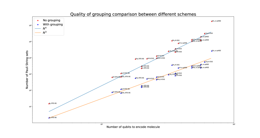
Figure 1: Top, number of commuting Pauli string sets, after cancellation and removal of zero coefficient terms, as a function of total number of Pauli strings. Bottom, number of commuting Pauli string sets as a function of number of qubits. The total number of Pauli strings is $O(N^{4})$ the orange curve shows that Baranyai grouping has achieved $O(N^{3})$ measurement complexity. It can be seen that this reduction is present in real Hamiltonians, not just idealised ones. The scatter around the trendlines is due to the number of zeros from symmetry being different in different molecules

IV.1 Other Mappings

Linear transformations between bases preserve commutativity of matrices acting on a vector space.[23]. This can also be seen from Equation 3 where $[A,B]$ denotes the commutator between $A$ and $B$, and $R$ denotes the coefficient map.

$$\begin{gathered}{[RAR^{-1},RBR^{-1}]}=R[A,B]R^{-1}\end{gathered}$$ (3)

Since the JW mapping is related to the Fock Space in a linear, invertible fashion, this grouping scheme is valid for any mapping that is a linear mapping of the Fock space. For example the Bravyi–Kitaev mapping, while a more complicated mapping from Fock space to qubit space, is still one to one and linear in the coefficients[24].

V Results

This solution was applied to 21 different molecular Hamiltonians for different molecules (H₂ – C₂H₆) and basis sets (STO-3G – cc-pVDZ)), and the results are shown in Figure 1 and tabulated in Table LABEL:Supp-tab:BaranyaiGroupingResult. The grouping showed a reduction in the number of terms from $O(N^{4})$ to $O(N^{3})$ on real, chemically relevant, Hamiltonians. The partitioning algorithm completed in a short time on a single core in Python, with the longest partitioning taking 2.5 hours and others taking minutes. Sparse linearly-scaling Hamiltonians were also tested and the resultant $O(1)$ group count is shown in Figure LABEL:Supp-fig:LinearHamiltonian in the Supplementary Information. The code is available as part of the FS-VQE framework[25, 26].

VI Conclusion

Here we showed that the Baranyai grouping produces small sets that scale with sparsity in the Hamiltonian. The algorithm completes in polynomial time and does not require significant computational effort. The implications of Hamiltonian partitioning into commuting sets can be used for simplifying VQE Pauli gadgets[27, 17], or Trotter expansions of Hamiltonian evolution circuits[28] by allowing multiple Pauli strings to be simultaneously diagonalised, which is necessary to perform the Rz rotations, reducing the number of diagonalising matrices and significantly lowering the depth of the circuit. Each commuting set generates other Pauli Strings which could be measured to reduce the variance[11] or Trotter error[13]. Anti-commuting sets can also be simultaneously measured, by non-Clifford rotations to a single Pauli string in the set[4], so by partitioning terms into either fully commuting or fully anti-commuting sets even fewer sets could be created.

VII Acknowledgements

The authors would like to give a special thanks to Lila Cadi Tazi for her scientific contribution, and to the entire Thom Group for their helpful discussions, and Nathan Fitzpatrick for helpful comments on the manuscript. We also thank the Royal Society of Chemistry for an RSC Undergraduate Research Bursary for this project.

VIII Author Declarations

The authors have no conflicts to disclose.
All authors contributed equally.

References

- Gokhale et al. [2019] P. Gokhale, O. Angiuli, Y. Ding, K. Gui, T. Tomesh, M. Suchara, M. Martonosi, and F. T. Chong, “Minimizing state preparations in variational quantum eigensolver by partitioning into commuting families,” (2019), arXiv:1907.13623 [quant-ph] .
- Inoue et al. [2023] W. Inoue, K. Aoyama, Y. Teranishi, K. Kanno, Y. O. Nakagawa, and K. Mitarai, “Almost optimal measurement scheduling of molecular Hamiltonian via finite projective plane,” (2023), arXiv:2301.07335 [quant-ph].
- Crawford et al. [2021] O. Crawford, B. van Straaten, D. Wang, T. Parks, E. Campbell, and S. Brierley, “Efficient quantum measurement of Pauli operators in the presence of finite sampling error,” Quantum 5, 385 (2021), arXiv:1908.06942 [quant-ph].
- Zhao et al. [2020] A. Zhao, A. Tranter, W. M. Kirby, S. F. Ung, A. Miyake, and P. J. Love, “Measurement reduction in variational quantum algorithms,” Physical Review A 101, 062322 (2020).
- Ralli et al. [2021] A. Ralli, P. J. Love, A. Tranter, and P. V. Coveney, “Implementation of measurement reduction for the variational quantum eigensolver,” Physical Review Research 3, 033195 (2021).
- Huang, Kueng, and Preskill [2020] H.-Y. Huang, R. Kueng, and J. Preskill, “Predicting many properties of a quantum system from very few measurements,” Nature Physics 16, 1050–1057 (2020).
- Izmaylov, Yen, and Ryabinkin [2019] A. F. Izmaylov, T.-C. Yen, and I. G. Ryabinkin, “Revising the measurement process in the variational quantum eigensolver: is it possible to reduce the number of separately measured operators?” Chemical Science 10, 3746–3755 (2019).
- Bonet-Monroig, Babbush, and O’Brien [2020] X. Bonet-Monroig, R. Babbush, and T. E. O’Brien, “Nearly Optimal Measurement Scheduling for Partial Tomography of Quantum States,” Physical Review X 10, 031064 (2020), arXiv:1908.05628 [quant-ph].
- Gokhale et al. [2020] P. Gokhale, O. Angiuli, Y. Ding, K. Gui, T. Tomesh, M. Suchara, M. Martonosi, and F. T. Chong, “ measurement cost for variational quantum eigensolver on molecular hamiltonians,” IEEE Transactions on Quantum Engineering 1, 1–24 (2020).
- Verteletskyi, Yen, and Izmaylov [2020] V. Verteletskyi, T.-C. Yen, and A. F. Izmaylov, “Measurement optimization in the variational quantum eigensolver using a minimum clique cover,” The Journal of Chemical Physics 152, 124114 (2020), https://pubs.aip.org/aip/jcp/article-pdf/doi/10.1063/1.5141458/15573883/124114_1_online.pdf .
- Choi, Yen, and Izmaylov [2022] S. Choi, T.-C. Yen, and A. F. Izmaylov, “Improving quantum measurements by introducing "ghost" Pauli products,” Journal of Chemical Theory and Computation 18, 7394–7402 (2022), arXiv:2208.06563 [physics, physics:quant-ph].
- Kohda et al. [2022] M. Kohda, R. Imai, K. Kanno, K. Mitarai, W. Mizukami, and Y. O. Nakagawa, “Quantum expectation-value estimation by computational basis sampling,” Physical Review Research 4, 033173 (2022), arXiv:2112.07416 [quant-ph].
- Choi and Izmaylov [2023] S. Choi and A. F. Izmaylov, “Measurement Optimization Techniques for Excited Electronic States in Near-Term Quantum Computing Algorithms,” Journal of Chemical Theory and Computation 19, 3184–3193 (2023), publisher: American Chemical Society.
- Jordan and Wigner [1928] P. Jordan and E. Wigner, “Über das Paulische Äquivalenzverbot,” Zeitschrift für Physik 47, 631–651 (1928).
- Sarkar and van den Berg [2019] R. Sarkar and E. van den Berg, “On sets of commuting and anticommuting paulis,” (2019), arXiv:1909.08123 [quant-ph] .
- Reggio et al. [2023] B. Reggio, N. Butt, A. Lytle, and P. Draper, “Fast partitioning of pauli strings into commuting families for optimal expectation value measurements of dense operators,” (2023), arXiv:2305.11847 [quant-ph] .
- Tazi and Thom [2023] L. C. Tazi and A. J. W. Thom, “Folded spectrum vqe : A quantum computing method for the calculation of molecular excited states,” (2023), arXiv:2305.04783 [quant-ph] .
- Baranyai [1979] Z. Baranyai, “The edge-coloring of complete hypergraphs i,” Journal of Combinatorial Theory, Series B 26, 276–294 (1979).
- Ford and Fulkerson [1956] L. R. Ford and D. R. Fulkerson, “Maximal flow through a network,” Canadian Journal of Mathematics 8, 399–404 (1956).
- Brouwer and Schrijver [1979] A. E. Brouwer and A. Schrijver, “Uniform hypergraphs,” In Packing and Covering in Combinatorics. Mathematical Centre Tracts , 39–73 (1979).
- Eisenstat [2014] D. Eisenstat, “Find unique compositions of k distinct element subsets for a set of n elements,” (2014).
- Kang and Payor [2015] D. Kang and J. Payor, “Flow Rounding,” (2015), arXiv:1507.08139 [cs].
- Choi, Jafarian, and Radjavi [1987] M. Choi, A. Jafarian, and H. Radjavi, “Linear maps preserving commutativity,” Linear Algebra and its Applications 87, 227–241 (1987).
- Tranter et al. [2018] A. Tranter, P. J. Love, F. Mintert, and P. V. Coveney, “A comparison of the bravyi–kitaev and jordan–wigner transformations for the quantum simulation of quantum chemistry,” Journal of Chemical Theory and Computation 14, 5617–5630 (2018), pMID: 30189144, https://doi.org/10.1021/acs.jctc.8b00450 .
- Lila C.T. [2023] B. C. Lila C.T., “Fs-vqe: Folded spectrum method implemented on a variational quantum eigensolver for the computation of molecular excited states.” (2023).
- Qiskit contributors [2023] Qiskit contributors, “Qiskit: An open-source framework for quantum computing,” (2023).
- Peruzzo et al. [2014] A. Peruzzo, J. McClean, P. Shadbolt, M.-H. Yung, X.-Q. Zhou, P. J. Love, A. Aspuru-Guzik, and J. L. O’Brien, “A variational eigenvalue solver on a photonic quantum processor,” Nature Communications 5 (2014), 10.1038/ncomms5213.
- Leadbeater et al. [2023] C. Leadbeater, N. Fitzpatrick, D. M. Ramo, and A. J. W. Thom, “Non-unitary trotter circuits for imaginary time evolution,” (2023), arXiv:2304.07917 [quant-ph] .