Nonlinear rigid-body quantization of Skyrmions

Abstract

We consider rigid-body quantization of the Skyrmion in the most general four-derivative generalization of the Skyrme model with a potential giving pions a mass, as well as in a class of higher-order Skyrme models. First of all, we find a way to quantize the spin and isospin zeromodes of the single Skyrmion corresponding to the nucleon, even though the theory contains more than two time derivatives. Although one could hope that a one-parameter family of theories could provide a smaller spin correction to the energy at some point in theory space – which would be welcome for BPS-type models, we find that the standard Skyrme model gives rise to the smallest spin correction to the energy and the other theories with more than two time-derivatives increase the kinetic energy due to the spin of the nucleon with respect to the standard Skyrme model. We speculate whether this tuning of the spin energy could be useful in the larger picture of quantizing vibrational and light massive modes of the Skyrmions.

I Introduction

The Skyrme model [1, 2] is a low-energy effective field theory description of QCD in a pure pion theory, where baryons are solitons known as Skyrmions. Although the model was proposed already in the sixties by Skyrme, it first received serious attention after Witten showed that the Skyrmion is the nucleon of QCD in the large-$N_{c}$ limit in the seminal papers [3, 4]. Although the Skyrme model provides a qualitative description of the nucleon to about the 30% level of accuracy compared with experiments [5], a major obstacle in using the theory for nuclei is that it gets the binding energies wrong by roughly an order of magnitude, already at the classical level. The community has worked on solving this problem at the classical level, essentially by finding so-called BPS limits of the theory, for which there exist solutions, the idea being that once one have found the BPS limit, a small perturbation could create the tiny binding energies of about 1% of the nucleon mass per baryon. To list a few of the attempts to find a BPS-type model for Skyrmions, the Sutcliffe model [6, 7] is a five-dimensional Yang-Mills theory that realizes a flat-space holographic description of Skyrmions as the holonomy of the gauge fields [8]; the BPS-Skyrme model is a radical change of the Skyrme model by eliminating the model and replacing it by the topological charge current squared as well as a suitable potential [9, 10]; finally, the weakly-bound Skyrme model is based on an energy bound using the Hölder inequality for which the Skyrme term and a potential to the fourth power saturates the energy bound [11, 12]. The Sutcliffe model requires an infinite number of vector bosons added to the Skyrme model in order to reach the BPS limit, i.e. the limit in which the classical energy is directly proportional to the baryon number, hence yielding vanishing classical binding energy. The advantage of the model, similarly to holographic constructions [13] and the hidden local symmetry approach [14], is that all the couplings to the infinite tower of vector bosons are determined. The BPS-Skyrme model has (analytic) solutions for any baryon number that saturates the Bogomol’nyi bound, but near-BPS solutions turn out to be a numerically challenging problem [12, 15, 16, 17]. The weakly-coupled Skyrme model only saturates the Bogomol’nyi bound for a single baryon, hence all nuclei already have a nonvanishing albeit small classical binding energy. It turns out that all the solutions take the shape of lattices of point-particle like Skyrmions [12]. For completeness, we can mention that a dielectric formulation of the Skyrme model [18] also provides small binding energies [18, 19], but also in this case the solutions tend to be point-particle like constellations like in the weakly-bound Skyrme model [19].

Now as put forward in the recent paper [20], although the BPS race that has taken place for over 10 years in the community has given rise to interesting ideas and some analytic solutions, the vanishing classical binding energy does not solve the problem of the binding energy of nuclei, simply due to the spin correction. In order to illustrate this, let’s consider the standard Skyrme model with the rational map approximation [21, 22]:

$$E=\int\mathop{}\!\mathrm{d}^{3}x\;\left[\lambda(a_{1}+a_{2}B)\mathcal{E}_{2}+\lambda^{-1}(b_{1}+b_{2}B)B\mathcal{E}_{4}\right],$$ (1)

with $a_{1,2}$, $b_{1,2}$ being positive coefficients, $B$ the baryon number and $\lambda$ the length scale. Finding the Derrick stability, we obtain

$$\lambda=\sqrt{\frac{e_{4}(b_{1}+b_{2}B)B}{e_{2}(a_{1}+a_{2}B)}},$$ (2)

which for large $B$ goes like $\lambda\propto\sqrt{B}$. The size of the Skyrmion hence grows like $\sqrt{B}$. Since the mass of the Skyrmion grows at least as fast as $B$, the moment of inertia scales like $B^{2}$ or higher. The spin correction to the energy found in the seminal paper by Adkins-Nappi-Witten thus goes like

$$E_{\rm spin}=\frac{J^{2}}{2\Lambda}\propto\frac{J^{2}}{B^{2}}.$$ (3)

Hence, even for nuclei whose ground state has a spin, the spin contribution is suppressed by roughly $B^{2}$ and quickly becomes negligible. Even more troublesome are the nuclei that are bosonic with spin 0 and isospin 0 in the ground state, as their contribution is just zero.

Now let us contemplate a BPS model, which by definition has vanishing classical binding energy for the Skyrmions. Using only rigid-body quantization, we can thus compute the binding energy of e.g. ⁴He as

$$\Delta=4(M_{1}+E_{\rm spin})-(4M_{1}+0)=\frac{3}{2\Lambda}.$$ (4)

Computing this number within the standard Skyrme model as a rough estimate, one obtains of the order of $4\times 4.6\%$ of the nucleon mass, which is about $175\operatorname{MeV}$. The physical binding energy of ⁴He is about $28.3\operatorname{MeV}$. For nuclei with nonvanishing spin and/or isospin in the ground state, the problem is, of course, slightly less severe.

We can thus see that the BPS models cannot solve the binding energy problem of the Skyrme model in the scheme of rigid-body quantization, as also explained in Ref. [20]. In the latter reference, it was proposed that since the number of zeromodes are fixed and independent of the baryon number, the quantum contribution is underestimated for $B>1$ nuclei and the resolution is to take more modes into account in the quantization procedure. We can now see that there are two ways to approach the problem: in the spirit of Ref. [20] one could take as many degrees of freedom as needed into account and quantize them to hopefully arrive at a cancellation of contributions that land just right on the nuclear physics scale of about $8\operatorname{MeV}$ per nucleon. Alternatively, one could believe in the semi-classical approximation of solitons being a good description of nature, with the classical contribution (mass) being the dominant one, and all quantum corrections being much smaller in magnitude, thus possibly avoiding too large cancellations (fine tuning) in the final result.

With the latter notion of naturalness in mind, which is also confirming the validity of using solitons in the first place, one may ask whether it is possible to lower the spin contribution to the nucleon. In this paper, we study this question in a generalization of the Skyrme model to the most general Lorentz-invariant Lagrangian written in terms of the chiral Lagrangian field $U\in\operatorname{SU}(2)$ with up to four derivatives and up to second order in a polynomial potential. Unfortunately, our result is, as it turns out, the Skyrme model limit of the model at hand gives the smallest spin contribution to the energy for the nucleon. For the naturalness path forward, one would thus stick with the Skyrme term, whereas if one proceeded along the cancellation path to nuclear phenomenology, this model introduces an extra parameter that could be used to fine tune the binding energies.

The paper is organized as follows. In Sec. II we introduce the generalization of the Skyrme model to the most general four-derivative theory and write down the spin contribution to the energy. In Sec. II.1 we give our chosen calibration scheme and in Sec. II.2 we present the numerical results of the paper. In Sec. III we include a class of higher-order Skyrme models with four time derivative and between 8 and 12 derivatives in total, whose quantization is identical to the model of Sec. II with modified moments of inertia. We conclude in Sec. IV with a discussion and outlook. We have delegated the details of the positivity of the energy of the model of Sec. II to App. A.

II The Skyrme model with all fourth-order derivative terms

We consider the chiral Lagrangian with the most general Lorentz-invariant Lagrangian, up to fourth order in derivatives [23, 24, 25, 26, 27], including the standard pion mass term [28], as well as the loosely bound potential term [29, 30]; hence the Lagrangian is also the most general Lagrangian up to polynomials of order 2, in the chiral Lagrangian field, $U$ [30]:

$$\mathcal{L} =\frac{F_{\pi}^{2}}{16}\operatorname{tr}(R_{\mu}R^{\mu})+\frac{1}{32e^{2}}\operatorname{tr}\left([R_{\mu},R_{\nu}][R^{\mu},R^{\nu}]\right)-\frac{\beta}{32}\left(\operatorname{tr}(R_{\mu}R^{\mu})\right)^{2}$$

$$\phantom{=\ }-\frac{F_{\pi}^{2}m_{\pi}^{2}}{8}\operatorname{tr}(\mathbf{1}_{2}-U)-\frac{F_{\pi}^{2}M^{2}}{32}\left[\operatorname{tr}(\mathbf{1}_{2}-U)\right]^{2},$$ (5)

where the right-invariant chiral current is

$$R_{\mu}=\partial_{\mu}UU^{\dagger},$$ (6)

$F_{\pi}$ is the pion decay constant, $e$ is the Skyrme coupling constant, $\beta$ is the dimensionless coupling of the other fourth-order derivative term which we shall dub the kinetic term squared, $m_{\pi}$ is the pion mass, $M$ is the mass parameter of the loosely bound potential term, the chiral Lagrangian or Skyrme field $U$ is related to the pions via

$$U=\mathbf{1}_{2}\sigma+\mathrm{i}\boldsymbol{\pi}\cdot\boldsymbol{\tau},$$ (7)

where $\boldsymbol{\tau}$ are the standard Pauli spin matrices, and finally we use the Minkowski metric with the mostly positive signature.

By the most general fourth-order derivative theory with only the field $U$, we mean that field redefinitions and integration-by-parts relations have been taken into account, leaving the two displayed terms as a representation of the two independent terms that exist, at this order in the derivative expansion [23, 24, 25, 26, 27].

The topological charge of the field $U$ is known as the baryon number and can be computed as

$$B=-\frac{1}{24\pi^{2}}\int\mathop{}\!\mathrm{d}^{3}x\;\epsilon^{ijk}\operatorname{tr}(R_{i}R_{j}R_{k}),$$ (8)

which arises due to the finite-energy condition on $U$ implying that $\lim_{|x|\to\infty}U=\mathbf{1}_{2}$ (or another constant, that however can be rotated into the unit matrix) which in turn effectively point-compactifies 3-space to $S^{3}$ and hence $\pi_{3}(\operatorname{SU}(2)_{\rm L}\times\operatorname{SU}(2)_{\rm R}/\operatorname{SU}(2)_{\rm diag})=\mathbb{Z}\ni B$.

We first redefine new dimensionless coupling constants as

$$\frac{1}{e^{2}}=\alpha^{2}(2\eta-1),\qquad\beta=2\alpha^{2}(1-\eta),\qquad\eta\in[0,1],$$ (9)

where $\eta$ interpolates between the two fourth-order soliton-stabilizing terms and $\alpha$ is an overall positive coefficient. For the details of the positivity of the static energy, see App. A. The Lagrangian now reads

$$\mathcal{L} =\frac{1}{2}\operatorname{tr}(R_{\mu}R^{\mu})+\frac{2\eta-1}{16}\operatorname{tr}\left([R_{\mu},R_{\nu}][R^{\mu},R^{\nu}]\right)-\frac{1-\eta}{8}\left(\operatorname{tr}(R_{\mu}R^{\mu})\right)^{2}$$

$$\phantom{=\ }-m_{1}^{2}\operatorname{tr}(\mathbf{1}_{2}-U)-\frac{m_{2}^{2}}{4}\left[\operatorname{tr}(\mathbf{1}_{2}-U)\right]^{2},$$ (10)

where the energy and length units are rescaled as

$$\mu=\frac{F_{\pi}\alpha}{4},\qquad\lambda=\frac{2\alpha}{F_{\pi}},$$ (11)

and the dimensionless mass parameters are given by

$$m_{1}:=\frac{2\alpha m_{\pi}}{F_{\pi}},\qquad m_{2}:=\frac{2\alpha M}{F_{\pi}}.$$ (12)

The real parameter $\eta$ interpolates between three different models, see Tab. 1.

	Skyrme term	kinetic term squared
$\eta=1$	1	0
$\eta=1/2$	0	$1/2$
$\eta=0$	$-1$	1

Table 1: A one-parameter family interpolating between 3 different models, with $\eta=1$ being the Skyrme model limit.

The Lagrangian splits into potential and kinetic energy as

$$L =T^{L}-V,$$ (13)

$$V =\int\mathop{}\!\mathrm{d}^{3}x\bigg{[}-\frac{1}{2}\operatorname{tr}(R_{i}^{2})-\frac{2\eta-1}{16}\operatorname{tr}\left([R_{i},R_{j}]^{2}\right)+\frac{1-\eta}{8}\left(\operatorname{tr}(R_{i}^{2})\right)^{2}$$

$$\phantom{=\int\mathop{}\!\mathrm{d}^{3}x\bigg{[}\ }+m_{1}^{2}\operatorname{tr}(\mathbf{1}_{2}-U)+\frac{m_{2}^{2}}{4}\left[\operatorname{tr}(\mathbf{1}_{2}-U)\right]^{2}\bigg{]},$$ (14)

$$T^{L} =\int\mathop{}\!\mathrm{d}^{3}x\bigg{[}-\frac{1}{2}\operatorname{tr}(R_{0}^{2})-\frac{2\eta-1}{8}\operatorname{tr}\left([R_{0},R_{i}]^{2}\right)-\frac{1-\eta}{8}\left(\operatorname{tr}(R_{0}^{2})\right)^{2}+\frac{1-\eta}{4}\operatorname{tr}(R_{0}^{2})\operatorname{tr}(R_{i}^{2})\bigg{]}.$$ (15)

Using the hedgehog Ansatz

$$U=\mathbf{1}_{2}\cos f(r)+\mathrm{i}\hat{\mathbf{x}}\cdot\boldsymbol{\tau}\sin f(r),$$ (16)

with $\hat{\mathbf{x}}=\mathbf{x}/r$ being a unit 3-vector in $\mathbb{R}^{3}$, $r=|\mathbf{x}|$ and the potential or static energy becomes

$$V =\int\mathop{}\!\mathrm{d}^{3}x\bigg{[}(f^{\prime})^{2}+\frac{2\sin^{2}f}{r^{2}}+(2\eta-1)\left(\frac{2\sin^{2}(f)(f^{\prime})^{2}}{r^{2}}+\frac{\sin^{4}f}{r^{4}}\right)$$

$$\phantom{=\int\mathop{}\!\mathrm{d}^{3}x\bigg{[}\ }+(1-\eta)\frac{\left(2\sin^{2}f+r^{2}(f^{\prime})^{2}\right)^{2}}{2r^{4}}+2m_{1}^{2}(1-\cos f)+m_{2}^{2}(1-\cos f)^{2}\bigg{]},$$ (17)

which is written such that the contributions from each term is visible. Simplifying the expression, we have

$$V =\int\mathop{}\!\mathrm{d}^{3}x\bigg{[}(f^{\prime})^{2}+\frac{2\sin^{2}f}{r^{2}}+\frac{1-\eta}{2}(f^{\prime})^{4}+2\eta\frac{\sin^{2}(f)(f^{\prime})^{2}}{r^{2}}+\frac{\sin^{4}f}{r^{4}}$$

$$\phantom{=\int\mathop{}\!\mathrm{d}^{3}x\bigg{[}\ }+2m_{1}^{2}(1-\cos f)+m_{2}^{2}(1-\cos f)^{2}\bigg{]},$$ (18)

which can be seen to be positive (semi-)definite, term by term, for $\eta\in[0,1]$.

The static equation of motion for the profile function of the Skyrmion is found by varying the static potential energy (18) with respect to $f$, yielding:

$$f^{\prime\prime}+\frac{2f^{\prime}}{r}-\frac{\sin 2f}{r^{2}}+3(1-\eta)(f^{\prime})^{2}f^{\prime\prime}+2(1-\eta)\frac{(f^{\prime})^{3}}{r}+\frac{2\eta\sin^{2}(f)f^{\prime\prime}}{r^{2}}\phantom{=0\ }$$

$$\mathop{+}\frac{\eta\sin(2f)(f^{\prime})^{2}}{r^{2}}-\frac{\sin^{2}(f)\sin 2f}{r^{4}}-m_{1}^{2}\sin f-m_{2}^{2}(1-\cos f)\sin f=0,$$ (19)

which needs to be accompanied by the boundary conditions $f(0)=\pi$ and $f(\infty)=0$.

Introducing a classical rotation of the spherically symmetric hedgehog Skyrmion can be done in two ways, either by isospinning the soliton

$$U^{(A)}(\mathbf{x},t)=A(t)U(\mathbf{x})A(t)^{\dagger},$$ (20)

which however is equivalent to spinning it via

$$U^{(A)}(\mathbf{x},t)=U(\mathsf{R}(t)\mathbf{x}),\qquad\mathsf{R}_{ij}=\frac{1}{2}\operatorname{tr}(\tau^{i}A\tau^{j}A^{\dagger}),$$ (21)

where $U(\mathbf{x})$ is a static solution to the field equations. The (classical) kinetic part of the Lagrangian can now readily be written down

$$T^{L} =\int\mathop{}\!\mathrm{d}^{3}x\bigg{[}-\frac{1}{2}\operatorname{tr}(T_{i}T_{j})-\frac{2\eta-1}{8}\operatorname{tr}\left([T_{i},R_{k}][T_{j},R_{k}]\right)+\frac{1-\eta}{4}\operatorname{tr}(T_{i}T_{j})\operatorname{tr}(R_{k}^{2})\bigg{]}a_{i}a_{j}$$

$$\phantom{=\ }+\int\mathop{}\!\mathrm{d}^{3}x\bigg{[}-\frac{1-\eta}{8}\operatorname{tr}(T_{i}T_{j})\operatorname{tr}(T_{k}T_{l})\bigg{]}a_{i}a_{j}a_{k}a_{l},$$ (22)

where $T_{i}=\frac{\mathrm{i}}{2}[\tau^{i},U]U^{\dagger}$ and the $\mathfrak{su}(2)$-valued angular momenta, $a_{i}\tau^{i}$, are defined as

$$a_{i}=-\mathrm{i}\operatorname{tr}(\tau^{i}A^{\dagger}\dot{A}).$$ (23)

In general, the kinetic energy is quite a complicated expression; however, for the spherically symmetric hedgehog Ansatz (16), the integrals reduce to

$$T=J_{i}a_{i}-T^{L}=\frac{1}{2}\Lambda_{1}a_{i}^{2}-\frac{3}{4}\Lambda_{2}a_{i}^{2}a_{j}^{2},$$ (24)

with the momentum conjugate to $a_{i}$:

$$J_{i}=\frac{\partial T^{L}}{\partial a_{i}}=\Lambda_{1}a_{i}-\Lambda_{2}(a_{j})^{2}a_{i}.$$ (25)

and

$$\Lambda_{1} =\frac{16\pi}{3}\int\mathop{}\!\mathrm{d}r\;r^{2}\bigg{[}\sin^{2}f+(2\eta-1)\sin^{2}f\left(\frac{\sin^{2}f}{r^{2}}+(f^{\prime})^{2}\right)$$

$$\phantom{=\frac{16\pi}{3}\int\mathop{}\!\mathrm{d}r\;r^{2}\bigg{[}\ }+2(1-\eta)\sin^{2}f\left(\frac{\sin^{2}f}{r^{2}}+\frac{1}{2}(f^{\prime})^{2}\right)\bigg{]},$$ (26)

$$\Lambda_{2} =(1-\eta)\frac{64\pi}{15}\int\mathop{}\!\mathrm{d}r\;r^{2}\sin^{4}f,$$ (27)

where we have used the following angular integrals

$$\int\mathop{}\!\mathrm{d}\theta\mathop{}\!\mathrm{d}\phi\;\sin\theta\hat{x}^{i}\hat{x}^{j}=\frac{4\pi}{3}\delta^{ij},\qquad\int\mathop{}\!\mathrm{d}\theta\mathop{}\!\mathrm{d}\phi\;\sin\theta\hat{x}^{i}\hat{x}^{j}\hat{x}^{k}\hat{x}^{l}=\frac{4\pi}{15}(\delta^{ij}\delta^{kl}+\delta^{ik}\delta^{jl}+\delta^{il}\delta^{jk}).$$

The expressions in $\Lambda_{1}$ are written out such that the contributions from the Skyrme term and the other fourth-order derivative term are distinguishable. Nevertheless, it will prove convenient to simplify the expression as

$$\Lambda_{1}=\frac{16\pi}{3}\int\mathop{}\!\mathrm{d}r\;r^{2}\left[\sin^{2}f+\eta\sin^{2}(f)(f^{\prime})^{2}+\frac{\sin^{4}f}{r^{2}}\right].$$ (28)

Since $\eta\in[0,1]$ and using the fact that every term is positive semi-definite, it is clear that $\Lambda_{1}$ takes the minimum value for $\eta=0$ and the maximum value for $\eta=1$ (ignoring the fact that the solution $f$ depends on $\eta$). There are two competing effects at play: Large $\eta$ increases the moment of inertia by increasing $\Lambda_{1}$, but it also decreases $\Lambda_{2}$, which reduces the moment of inertia by the quartic kinetic term.

Although it is difficult to compute $a_{i}$ in terms of $J_{i}$ of Eq. (25), the squared quantities are easier to handle:

$$J^{2}=\Lambda_{1}^{2}a^{2}+\Lambda_{2}^{2}(a^{2})^{3}-2\Lambda_{1}\Lambda_{2}(a^{2})^{2}.$$ (29)

We can now invert the equation by treating the equation as a classical cubic polynomial in $a^{2}$. Before solving the equation, it will prove useful to analyze the polynomial a bit before doing so. Let us write

$$y(x)=\Lambda_{2}^{2}x^{3}-2\Lambda_{1}\Lambda_{2}x^{2}+\Lambda_{1}^{2}x-J^{2},\qquad x:=a^{2}.$$ (30)

We find the saddle points straight forwardly as $y^{\prime}(x)=0$:

$$x_{\pm}=\left(\frac{2}{3}\pm\frac{1}{3}\right)\frac{\Lambda_{1}}{\Lambda_{2}},$$ (31)

which are both positive. The values of the polynomial function $y(x_{\pm})$ at the saddle points determine the number and kind of roots the polynomial possesses. In particular, we get

$$y(x_{-})=\frac{4\Lambda_{1}^{3}}{27\Lambda_{2}}-J^{2},\qquad y(x_{+})=-J^{2}.$$ (32)

The first (in the $x$-direction) saddle point value can change sign depending on the values of the integrals $\Lambda_{1}$ and $\Lambda_{2}$. Since $\Lambda_{1}$ is an increasing function with $\eta$ and $\Lambda_{2}$ is a decreasing function with $\eta$, the ratio $\Lambda_{1}^{3}/\Lambda_{2}$ is an increasing function with $\eta$, that diverges at $\eta=1$. This means that for large $\eta\sim 1$, $y(x_{-})$ is positive and $y(x_{+})$ is negative. In this case, there are 3 real roots of $y$, which is physically puzzling. There may or may not exist a critical value of $\eta=\eta^{\rm crit}$ for which $y(x_{-})<0$ is strictly negative; in this case, there will be only one real root of $y$ at $x>x_{+}$. In this case, the physical interpretation is straightforward; the root is inserted in the kinetic energy (24) and quantization of the spin degrees of freedom will have the eigenvalues of $J^{2}$ as $j(j+1)$ with $j=\tfrac{1}{2}$ for the nucleon.

In order to reach the form for which Cardano’s result applies, we shift the variable as $x=\xi+\frac{2\Lambda_{1}}{3\Lambda_{2}}$, for which the polynomial reads

$$\frac{y}{\Lambda_{2}^{2}}=\xi^{3}-\frac{\Lambda_{1}^{2}}{3\Lambda_{2}^{2}}\xi+\frac{2\Lambda_{1}^{3}}{27\Lambda_{2}^{3}}-\frac{J^{2}}{\Lambda_{2}^{2}}.$$ (33)

It will be convenient to define the coefficients

$$\ell=\frac{\Lambda_{1}}{\Lambda_{2}},\qquad\varsigma=\sqrt{\frac{27}{2}}\frac{J}{\Lambda_{2}},$$ (34)

for which we have three roots of $y$ as

$$\xi_{0,\pm}=\frac{2\ell}{3}\cos\left(\frac{\theta-\pi\pm 2\pi}{3}\right),\qquad\theta=\arctan\left(\frac{\varsigma\sqrt{2\ell^{3}-\varsigma^{2}}}{\ell^{3}-\varsigma^{2}}\right),$$ (35)

where the index $0$ means that $\pm 2\pi$ in the cosine is replaced by $0$ and

$$x_{0,\pm}=\xi_{0,\pm}+\frac{2}{3}\ell,$$ (36)

with $x_{-}$ being the smallest positive root.

Writing the kinetic quantum energy in terms of $J^{2}$, we get

$$T=\frac{1}{2}\Lambda_{1}x_{a}-\frac{3}{4}\Lambda_{2}x_{a}^{2},$$ (37)

with $x_{a}$, $a=0,\pm$ being one of the roots.

It turns out that after restoring units, $\varsigma$ is not always smaller than $\ell$, although this is true near the Skyrme limit ($\eta\to 1$). A good expansion parameter (possibly the only one) will be to expand in $1/\ell$, since $\ell>1$; more precisely, $1/\ell\sim 10^{-1}$ or smaller. Expanding in $1/\ell$, we obtain

$$\theta=\frac{\sqrt{2}\varsigma}{\ell^{3/2}}+\frac{\varsigma^{3}}{6\sqrt{2}\ell^{9/2}}+\frac{3\varsigma^{5}}{80\sqrt{2}\ell^{15/2}}+\frac{5\varsigma^{7}}{448\sqrt{2}\ell^{21/2}}+\mathcal{O}(\ell^{-25/2}),$$ (38)

which in turn yields

$$x_{-} =\frac{2\varsigma^{2}}{27\ell^{2}}+\frac{8\varsigma^{4}}{729\ell^{5}}+\frac{56\varsigma^{6}}{19683\ell^{8}}+\frac{160\varsigma^{8}}{177147\ell^{11}}+\mathcal{O}(\ell^{-23/2}),$$ (39)

$$x_{0,+} =\ell\pm\sqrt{\frac{2}{3\ell}}\frac{\varsigma}{3}-\frac{\varsigma^{2}}{27\ell^{2}}\pm\frac{5\varsigma^{3}}{162\sqrt{6}\ell^{7/2}}-\frac{4\varsigma^{4}}{729\ell^{5}}+\mathcal{O}(\ell^{-13/2}),$$ (40)

where the upper sign is for $x_{0}$ and the lower for $x_{+}$. Inserting the definitions (34), we obtain

$$x_{-} =\frac{J^{2}}{\Lambda_{1}^{2}}+\frac{2\Lambda_{2}J^{4}}{\Lambda_{1}^{5}}+\frac{7\Lambda_{2}^{2}J^{6}}{\Lambda_{1}^{8}}+\frac{30\Lambda_{2}^{3}J^{8}}{\Lambda_{1}^{11}}+\mathcal{O}\left(\frac{J^{10}\Lambda_{2}^{4}}{\Lambda_{1}^{14}}\right),$$ (41)

$$x_{0,+} =\frac{\Lambda_{1}}{\Lambda_{2}}\pm\frac{|J|}{\sqrt{\Lambda_{1}\Lambda_{2}}}-\frac{J^{2}}{2\Lambda_{1}^{2}}\pm\frac{5\Lambda_{2}^{1/2}|J|^{3}}{8\Lambda_{1}^{7/2}}-\frac{\Lambda_{2}J^{4}}{\Lambda_{1}^{5}}+\mathcal{O}\left(\frac{|J|^{5}\Lambda_{2}^{3/2}}{\Lambda_{1}^{13/2}}\right).$$ (42)

In the Skyrme limit, $\eta\to 1$ and $\Lambda_{2}\to 0$ so both $x_{+}$ and $x_{0}$ diverge with a splitting that also diverges, but slower (i.e. like $1/\sqrt{\Lambda_{2}}$).

Inserting the roots into the kinetic energy formula (37):

$$T(x_{-}) =\frac{J^{2}}{2\Lambda_{1}}+\frac{\Lambda_{2}J^{4}}{4\Lambda_{1}^{4}}+\frac{\Lambda_{2}^{2}J^{6}}{2\Lambda_{1}^{7}}+\frac{3\Lambda_{2}^{3}J^{8}}{2\Lambda_{1}^{10}}+\mathcal{O}\left(\frac{J^{10}\Lambda_{2}^{4}}{\Lambda_{1}^{13}}\right),$$ (43)

$$T(x_{0,+}) =-\frac{\Lambda_{1}^{2}}{4\Lambda_{2}}\mp\sqrt{\frac{\Lambda_{1}}{\Lambda_{2}}}|J|-\frac{J^{2}}{4\Lambda_{1}}\pm\frac{\Lambda_{2}^{1/2}|J|^{3}}{8\Lambda_{1}^{5/2}}-\frac{\Lambda_{2}J^{4}}{8\Lambda_{1}^{4}}+\mathcal{O}\left(\frac{|J|^{5}\Lambda_{2}^{3/2}}{\Lambda_{1}^{11/2}}\right),$$ (44)

we obtain the order-$\Lambda_{2}$ correction to the usual Skyrme model’s spin energy for the case of the smallest root, i.e. $T(x_{-})$, plus higher-order corrections. We will confirm with explicit computations that the series converges rather slowly and therefore we have expanded the energy $T(x_{-})$ up to order $J^{8}$. The term $-\Lambda_{1}^{2}/4\Lambda_{2}$ in $T(x_{0,+})$ already signals that the two cases of $x_{0}$ and $x_{+}$ are unphysical. In particular, they are both negative for $\Lambda_{1,2}$ computed with the model data.

The unfortunate thing about the above result, is that the spin energy for the lowest (and physical) kinetic energy, $T(x_{-})$, is only increased by the presence of a nonvanishing $\Lambda_{2}$, since this correction term is positive definite (and so are all the subleading corrections). The only possibility of lowering the spin correction to the mass, would be if the change in $\eta$ would increase $\Lambda_{1}$ much faster than it would increase $\Lambda_{2}$. However, dialing down $\eta$ from $\eta=1$, $\Lambda_{2}$ does increase, but $\Lambda_{1}$ tends to decrease. Already before performing computations, we can conclude that the Skyrme-model limit is the 4-derivative model with the lowest spin energy, which translates into the lowest minimal binding energy. We will confirm this statement with explicit computations.

In order to restore the units, we have to substitute $\Lambda_{1}\to\mu\lambda^{2}\Lambda_{1}$ and $\Lambda_{2}\to\mu\lambda^{4}\Lambda_{2}$. This means that $\ell\to\lambda^{-2}\ell$ and $\varsigma\to\mu^{-1}\lambda^{-4}\varsigma$, so even though $\theta$ of Eq. (35) is dimensionless, it depends on the calibration and in particular on $\mu\lambda=\alpha^{2}/2$. This is not per se surprising, since $\mu\lambda$ is our $1/\hbar$ and is expected to show up in the quantization; unfortunately, it means that one cannot calculate the dimensionless roots without first choosing a calibration. Restoring the units we obtain for the physical spin contribution to the energy:

$$T(x_{-}) =\frac{J^{2}}{2\mu\lambda^{2}\Lambda_{1}}+\frac{\Lambda_{2}J^{4}}{4\mu^{3}\lambda^{4}\Lambda_{1}^{4}}+\frac{\Lambda_{2}^{2}J^{6}}{2\mu^{5}\lambda^{6}\Lambda_{1}^{7}}+\frac{3\Lambda_{2}^{3}J^{8}}{2\mu^{7}\lambda^{8}\Lambda_{1}^{10}}+\mathcal{O}\left(\frac{J^{10}\Lambda_{2}^{4}}{\mu^{9}\lambda^{10}\Lambda_{1}^{13}}\right).$$ (45)

Clearly every term has the units of energy, as it should.

II.1 Calibration

In order to compare the quantum spin energy to the classical mass of the Skyrmion, we must calibrate the model. More precisely, $\alpha$ must be determined since the ratio of the quantum spin energy to the classical mass depends on it. The overall energy scale depends on $F_{\pi}$.

If we choose to fit the nucleon mass to the classical Skyrmion mass and the size of the Skyrmion to the electric charge radius of the nucleon, we obtain the following equations

$$\mu E=M_{N},\qquad\lambda R=R_{N}.$$ (46)

Solving for the pion decay constant and $\alpha$, we have

$$F_{\pi}=\frac{2R}{R_{N}}\alpha,\qquad\alpha=\sqrt{\frac{2M_{N}R_{N}}{ER}}.$$ (47)

We choose to fit the classical Skyrmion mass, since including the spin correction is complicated by the fact that the nontrivial and nonlinear $\alpha$ dependence makes an analytic formula unavailable. If one were to choose to fit the total Skyrmion mass to the physical mass, only numerical methods would be able to do so. Since we know that there are further corrections to the Skyrmion energy, e.g. from vibrational modes [31], we simplify the problem and fit just to the classical Skyrmion mass here.

II.2 Numerical results

We solve the equation of motion (19) for the static Skyrmion, and use it to compute the two moments of “inertia”, $\Lambda_{1,2}$ of Eqs. (27)-(28). We use simple gradient flow as the numerical method. Then we use Eq. (47) to calibrate the model, which in turn determines the energy and length scale (11). With these at hand, and using the appropriate spin of the nucleon $j=1/2$ yielding $J^{2}=3/4$, we can compute the spin correction to the energy using Eq. (45) and other observables of the model.

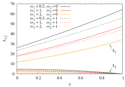
(a)

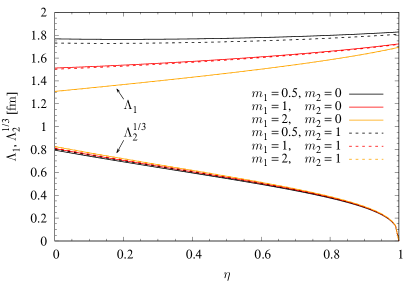
(b)

Figure 1: (a) The moments of inertia $\Lambda_{1}$, $\Lambda_{2}$ as functions of $\eta$ for a range of the pion mass parameter $m_{1}=0.5,1,2$ with and without the loosely bound potential turned on $m_{2}=0,1$. (b) The moments of inertia after restoring physical units: $\mu\lambda^{2}\Lambda_{1}$ and $(\mu\lambda^{4}\Lambda_{2})^{1/3}$.

In Fig. 1, the moments of inertia $\Lambda_{1,2}$ are shown. It is clearly visible that the dimensionless ratio $\Lambda_{1}/\Lambda_{2}>1$, which is a necessary condition for the validity of the expansion in $\Lambda_{2}/\Lambda_{1}$.

(a)

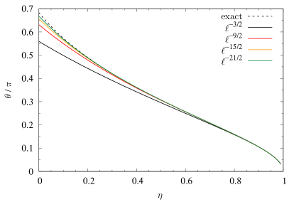
(b)

Figure 2: (a) The physical spin correction to the energy $T$ as function of $\eta$ for a range of the pion mass parameter $m_{1}=0.5,1,2$ with and without the loosely bound potential turned on $m_{2}=0,1$. For simplicity we denote the order in terms of the powers of $J$, although the expansion is not an expansion in terms of $J$, but in terms of $\ell^{-1}$. (b) The angle $\theta$ of Eq. (35) as a function of $\eta$.

In Fig. 2(b) is shown the angle $\theta$ and although the angle is not small over the entire range of $\eta\in[0,1]$ (it only is so for $\eta\sim 1$), the convergence in the $\ell^{-1}$ expansion is demonstrated. Fig. 2(a) shows the spin correction to the energy for the smallest root, which is the physical case and the root that smoothly connects to the single root present in the Skyrme model limit $\eta\to 1$. The convergence of the spin correction to the energy is observed to be slower in the $\ell^{-1}$ expansion with respect to $\theta$.

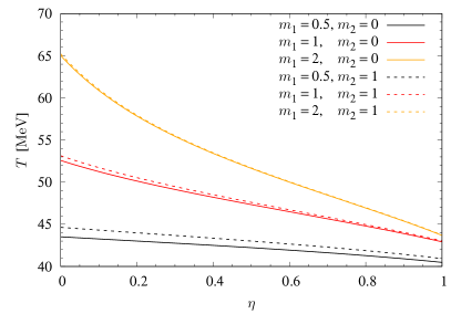
(a)

Figure 3: The spin correction to the energy at order $J^{8}$ as functions of $\eta$ for a range of the pion mass parameter $m_{1}=0.5,1,2$ with and without the loosely bound potential turned on $m_{2}=0,1$.

In Fig. 3 we show the spin correction to the energy as a function of $\eta$ for various pion mass and loosely bound potential parameters. The fit (47) employed here amounts to the classical mass of the Skyrmion always being at the experimental face value and so the spin correction should be as small as possible. Re-calibration could of course get the nucleon mass right, but as discussed in the introduction, the larger the spin energy is, the larger the binding energies are. Since they should physically be around $8\operatorname{MeV}$ for larger nuclei, a spin correction to the energy much larger than that creates tension and warrants other (extended) quantization methods to provide physical spectra, see e.g. Ref. [20]. We note that the dependence of the spin correction on the pion mass parameter $m_{1}$ is quite large, whereas the dependence on the loosely bound potential parameter $m_{2}$ is only mild.

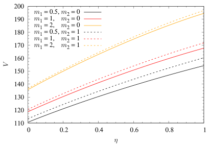
(a)

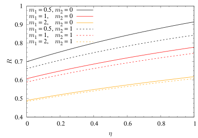
(b)

Figure 4: (a) The static energy of the Skyrmion and (b) the (charge) radius of the Skyrmion, both as functions of $\eta$ for a range of the pion mass parameter $m_{1}=0.5,1,2$ with and without the loosely bound potential turned on $m_{2}=0,1$.

Fig. 4 shows the static classical mass and radius of the Skyrmion in dimensionless (model) units. In physical units, the classical mass and radius are exactly equal to their experimental values, $939\operatorname{MeV}$ and $0.8783\operatorname{fm}$, respectively, due to the calibration of the model (47).

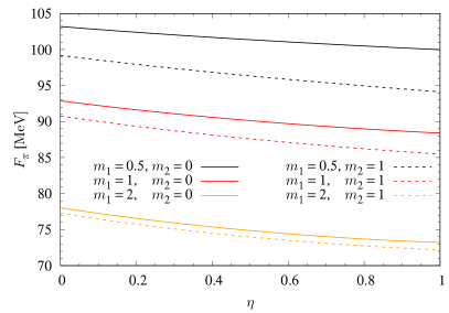
(a)

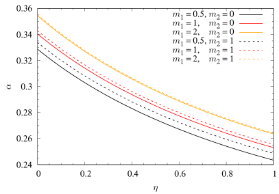
(b)

Figure 5: (a) The pion decay constant and (b) the four-derivative coupling constant $\alpha$, both as functions of $\eta$ for a range of the pion mass parameter $m_{1}=0.5,1,2$ with and without the loosely bound potential turned on $m_{2}=0,1$. The physical value of the pion decay constant in the normalization used in this paper is $186\operatorname{MeV}$.

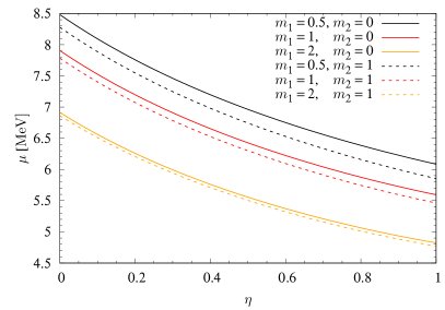
(a)

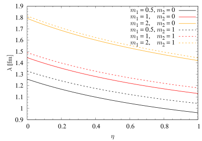
(b)

Figure 6: The calibrated (a) energy scale and (b) length scale of the model, both as functions of $\eta$ for a range of the pion mass parameter $m_{1}=0.5,1,2$ with and without the loosely bound potential turned on $m_{2}=0,1$.

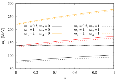
Figure 7: The pion mass as a function of $\eta$ for a range of the pion mass parameter $m_{1}=0.5,1,2$ with and without the loosely bound potential turned on $m_{2}=0,1$. The physical value of the pion mass is around $139\operatorname{MeV}$ (ignoring isospin breaking effects) and is shown with a dotted horizontal black line.

Having the classical mass and radius of the Skyrmion in hand, we thus readily calibrate the model according to Eq. (47), yielding the pion decay constant in Fig. 5(a), the four-derivative term coupling constant $\alpha$ in Fig. 5(b) or equivalently the energy scale $\mu$ in Fig. 6(a) and the length scale $\lambda$ in Fig. 6(b). For completeness, we plot the pion mass in Fig. 7, from which we can see that the pion mass parameter should be taken somewhere between $0.75$ and $1$, depending on the values of $\eta$ and $m_{2}$, in order to reproduce the experimental value of roughly $139\operatorname{MeV}$.

III Higher-order Skyrme models

We now consider the cases of the higher-order models introduced in Ref. [32], i.e. higher-order derivative theories with four time derivatives and with eight to twelve derivatives in total. The Lagrangian reads

$$\mathcal{L} =\frac{F_{\pi}^{2}}{16}\operatorname{tr}(R_{\mu}R^{\mu})+\frac{1}{32e^{2}}\operatorname{tr}\left([R_{\mu},R_{\nu}][R^{\mu},R^{\nu}]\right)+\mathcal{L}^{\prime}$$

$$\phantom{=\ }-\frac{F_{\pi}^{2}m_{\pi}^{2}}{8}\operatorname{tr}(\mathbf{1}_{2}-U)-\frac{F_{\pi}^{2}M^{2}}{32}\left[\operatorname{tr}(\mathbf{1}_{2}-U)\right]^{2},$$ (48)

with the new higher-derivative term $\mathcal{L}^{\prime}$ being one of the four possibilities:

$$\mathcal{L}_{8a} =-\frac{\beta_{8}}{1024F_{\pi}^{4}}\left(\operatorname{tr}\left([R_{\mu},R_{\nu}][R^{\mu},R^{\nu}]\right)\right)^{2},$$ (49)

$$\mathcal{L}_{8b} =-\frac{\beta_{8}}{1536F_{\pi}^{4}}\operatorname{tr}(R_{\sigma}R^{\sigma})\operatorname{tr}\left([R_{\mu},R^{\nu}][R_{\nu},R^{\rho}][R_{\rho},R^{\mu}]\right),$$ (50)

$$\mathcal{L}_{10} =-\frac{\beta_{10}}{3072F_{\pi}^{6}}\operatorname{tr}\left([R_{\sigma},R_{\delta}][R^{\sigma},R^{\delta}]\right)\operatorname{tr}\left([R_{\mu},R^{\nu}][R_{\nu},R^{\rho}][R_{\rho},R^{\mu}]\right),$$ (51)

$$\mathcal{L}_{12} =-\frac{\beta_{12}}{9216F_{\pi}^{8}}\left(\operatorname{tr}\left([R_{\mu},R^{\nu}][R_{\nu},R^{\rho}][R_{\rho},R^{\mu}]\right)\right)^{2}.$$ (52)

We first define the relations to the coupling $\eta$:

$$\frac{1}{e^{2}}=\alpha^{2}\eta,\qquad\beta_{n}=\big{(}\sqrt{2}\alpha\big{)}^{n-2}(1-\eta).$$ (53)

Rescaling the Lagrangians to the energy and length units (11) yields the dimensionless Lagrangian

$$\mathcal{L} =\frac{1}{2}\operatorname{tr}(R_{\mu}R^{\mu})+\frac{\eta}{16}\operatorname{tr}\left([R_{\mu},R_{\nu}][R^{\mu},R^{\nu}]\right)+\mathcal{L}^{\prime}$$

$$\phantom{=\ }-m_{1}^{2}\operatorname{tr}(\mathbf{1}_{2}-U)-\frac{m_{2}^{2}}{4}\left[\operatorname{tr}(\mathbf{1}_{2}-U)\right]^{2},$$ (54)

with the dimensionless higher-order term $\mathcal{L}^{\prime}$ being one of the following four terms:

$$\mathcal{L}_{8a} =-\frac{1-\eta}{1024}\left(\operatorname{tr}\left([R_{\mu},R_{\nu}][R^{\mu},R^{\nu}]\right)\right)^{2},$$ (55)

$$\mathcal{L}_{8b} =-\frac{1-\eta}{1536}\operatorname{tr}(R_{\sigma}R^{\sigma})\operatorname{tr}\left([R_{\mu},R^{\nu}][R_{\nu},R^{\rho}][R_{\rho},R^{\mu}]\right),$$ (56)

$$\mathcal{L}_{10} =-\frac{1-\eta}{6144}\operatorname{tr}\left([R_{\sigma},R_{\delta}][R^{\sigma},R^{\delta}]\right)\operatorname{tr}\left([R_{\mu},R^{\nu}][R_{\nu},R^{\rho}][R_{\rho},R^{\mu}]\right),$$ (57)

$$\mathcal{L}_{12} =-\frac{1-\eta}{36864}\left(\operatorname{tr}\left([R_{\mu},R^{\nu}][R_{\nu},R^{\rho}][R_{\rho},R^{\mu}]\right)\right)^{2}.$$ (58)

Splitting the Lagrangians up into potential and kinetic terms, we get

$$L =T^{L}-V,$$ (59)

$$V =\int\mathop{}\!\mathrm{d}^{3}x\bigg{[}-\frac{1}{2}\operatorname{tr}(R_{i}^{2})-\frac{\eta}{16}\operatorname{tr}\left([R_{i},R_{j}]^{2}\right)+m_{1}^{2}\operatorname{tr}(\mathbf{1}_{2}-U)+\frac{m_{2}^{2}}{4}\left[\operatorname{tr}(\mathbf{1}_{2}-U)\right]^{2}\bigg{]}+V^{\prime},$$ (60)

$$T^{L} =\int\mathop{}\!\mathrm{d}^{3}x\bigg{[}-\frac{1}{2}\operatorname{tr}(T_{i}T_{j})-\frac{\eta}{8}\operatorname{tr}\left([T_{i},R_{k}][T_{j},R_{k}]\right)\bigg{]}a_{i}a_{j}+{T^{L}}^{\prime},$$ (61)

with potential terms

$$V_{8a} =\frac{1-\eta}{1024}\int\mathop{}\!\mathrm{d}^{3}x\left(\operatorname{tr}\left([R_{i},R_{j}]^{2}\right)\right)^{2},$$ (62)

$$V_{8b} =\frac{1-\eta}{1536}\int\mathop{}\!\mathrm{d}^{3}x\operatorname{tr}(R_{l}^{2})\operatorname{tr}\left([R_{i},R_{j}][R_{j},R_{k}][R_{k},R_{i}]\right),$$ (63)

$$V_{10} =\frac{1-\eta}{6144}\int\mathop{}\!\mathrm{d}^{3}x\operatorname{tr}\left([R_{k},R_{l}]^{2}\right)\operatorname{tr}\left([R_{i},R_{j}][R_{j},R_{k}][R_{k},R_{i}]\right),$$ (64)

$$V_{12} =\frac{1-\eta}{36864}\int\mathop{}\!\mathrm{d}^{3}x\;\big{(}\operatorname{tr}\left([R_{i},R_{j}][R_{j},R_{k}][R_{k},R_{i}]\right)\big{)}^{2},$$ (65)

and kinetic terms

$$T_{8a} =\frac{1-\eta}{256}\int\mathop{}\!\mathrm{d}^{3}x\;\operatorname{tr}\left([T_{i},R_{k}][T_{j},R_{k}]\right)\operatorname{tr}\left([R_{l},R_{m}]^{2}\right)a_{i}a_{j}$$

$$\phantom{=\ }-\frac{1-\eta}{256}\int\mathop{}\!\mathrm{d}^{3}x\;\operatorname{tr}\left([T_{i},R_{m}][T_{j},R_{m}]\right)\operatorname{tr}\left([T_{k},R_{n}][T_{l},R_{n}]\right)a_{i}a_{j}a_{k}a_{l},$$ (66)

$$T_{8b} =\frac{1-\eta}{1536}\int\mathop{}\!\mathrm{d}^{3}x\Big{[}\operatorname{tr}(T_{i}T_{j})\operatorname{tr}\left([R_{k},R_{l}][R_{l},R_{m}][R_{m},R_{k}]\right)$$

$$\phantom{=\frac{1-\eta}{1536}\int\mathop{}\!\mathrm{d}^{3}x\Big{[}\ }+3\operatorname{tr}(R_{m}^{2})\operatorname{tr}\left([T_{i},R_{k}][R_{k},R_{l}][R_{l},T_{j}]\right)\Big{]}a_{i}a_{j}$$

$$\phantom{=\ }-\frac{1-\eta}{512}\int\mathop{}\!\mathrm{d}^{3}x\;\operatorname{tr}(T_{i}T_{j})\operatorname{tr}\left([T_{k},R_{m}][R_{m},R_{n}][R_{n},T_{l}]\right)a_{i}a_{j}a_{k}a_{l},$$ (67)

$$T_{10} =\frac{1-\eta}{6144}\int\mathop{}\!\mathrm{d}^{3}x\Big{[}2\operatorname{tr}\left([T_{i},R_{k}][T_{j},R_{k}]\right)\operatorname{tr}\left([R_{l},R_{m}][R_{m},R_{n}][R_{n},R_{l}]\right)$$

$$\phantom{=\frac{1-\eta}{6144}\int\mathop{}\!\mathrm{d}^{3}x\Big{[}\ }+3\operatorname{tr}\left([R_{m},R_{n}]^{2}\right)\operatorname{tr}\left([T_{i},R_{k}][R_{k},R_{l}][R_{l},T_{j}]\right)\Big{]}a_{i}a_{j}$$

$$\phantom{=\ }-\frac{1-\eta}{1024}\int\mathop{}\!\mathrm{d}^{3}x\;\operatorname{tr}\left([T_{i},R_{o}][T_{j},R_{o}]\right)\operatorname{tr}\left([T_{k},R_{m}][R_{m},R_{n}][R_{n},T_{l}]\right)a_{i}a_{j}a_{k}a_{l},$$ (68)

$$T_{12} =\frac{1-\eta}{6144}\int\mathop{}\!\mathrm{d}^{3}x\;\operatorname{tr}\left([T_{i},R_{k}][R_{k},R_{l}][R_{l},T_{j}]\right)\operatorname{tr}\left([R_{m},R_{n}][R_{o},R_{p}][R_{p},R_{m}]\right)a_{i}a_{j}$$

$$\phantom{=\ }-\frac{1-\eta}{4096}\int\mathop{}\!\mathrm{d}^{3}x\;\operatorname{tr}\left([T_{i},R_{m}][R_{m},R_{n}][R_{n},T_{j}]\right)\operatorname{tr}\left([T_{k},R_{o}][R_{o},R_{p}][R_{p},T_{l}]\right)a_{i}a_{j}a_{k}a_{l},$$ (69)

and $T_{i}=\frac{\mathrm{i}}{2}[\tau^{i},U]U^{\dagger}$ as always. Inserting the hedgehog Ansatz (16), we obtain the potential term

$$V =\int\mathop{}\!\mathrm{d}^{3}x\bigg{[}(f^{\prime})^{2}+\frac{2\sin^{2}f}{r^{2}}+\eta\frac{\sin^{2}f}{r^{4}}\left(\sin^{2}f+2r^{2}(f^{\prime})^{2}\right)$$

$$\phantom{=\int\mathop{}\!\mathrm{d}^{3}x\bigg{[}\ }+2m_{1}^{2}(1-\cos f)+m_{2}^{2}(1-\cos f)^{2}\bigg{]}+V^{\prime}$$ (70)

with

$$V_{8a} =\frac{1-\eta}{4}\int\mathop{}\!\mathrm{d}^{3}x\;\frac{\sin^{4}f}{r^{8}}\left(\sin^{2}f+2r^{2}(f^{\prime})^{2}\right)^{2},$$ (71)

$$V_{8b} =\frac{1-\eta}{8}\int\mathop{}\!\mathrm{d}^{3}x\;\frac{\sin^{4}(f)(f^{\prime})^{2}}{r^{6}}\left(2\sin^{2}f+r^{2}(f^{\prime})^{2}\right),$$ (72)

$$V_{10} =\frac{1-\eta}{4}\int\mathop{}\!\mathrm{d}^{3}x\;\frac{\sin^{6}(f)(f^{\prime})^{2}}{r^{8}}\left(\sin^{2}f+2r^{2}(f^{\prime})^{2}\right),$$ (73)

$$V_{12} =\frac{1-\eta}{4}\int\mathop{}\!\mathrm{d}^{3}x\;\frac{\sin^{8}(f)(f^{\prime})^{4}}{r^{8}},$$ (74)

whereas for the kinetic term we get

$$T^{L}=\frac{1}{2}\Lambda_{1}a_{i}^{2}-\frac{1}{4}\Lambda_{2}^{\prime}a_{i}^{2}a_{j}^{2},$$ (75)

with

$$\Lambda_{1}=\frac{16\pi}{3}\int\mathop{}\!\mathrm{d}r\;r^{2}\bigg{[}\sin^{2}f+\eta\sin^{2}f\left(\frac{\sin^{2}f}{r^{2}}+(f^{\prime})^{2}\right)\bigg{]}+\Lambda_{1}^{\prime},$$ (76)

and

$$\Lambda_{1}^{(8a)} =\frac{8\pi(1-\eta)}{3}\int\mathop{}\!\mathrm{d}r\;\frac{\sin^{4}f}{r^{4}}\left(\sin^{2}f+r^{2}(f^{\prime})^{2}\right)\left(\sin^{2}f+2r^{2}(f^{\prime})^{2}\right),$$ (77)

$$\Lambda_{1}^{(8b)} =\frac{2\pi(1-\eta)}{3}\int\mathop{}\!\mathrm{d}r\;\frac{\sin^{4}(f)(f^{\prime})^{2}}{r^{2}}\left(3\sin^{2}f+r^{2}(f^{\prime})^{2}\right),$$ (78)

$$\Lambda_{1}^{(10)} =\frac{4\pi(1-\eta)}{3}\int\mathop{}\!\mathrm{d}r\;\frac{\sin^{6}(f)(f^{\prime})^{2}}{r^{4}}\left(2\sin^{2}f+3r^{2}(f^{\prime})^{2}\right),$$ (79)

$$\Lambda_{1}^{(10)} =\frac{8\pi(1-\eta)}{3}\int\mathop{}\!\mathrm{d}r\;\frac{\sin^{8}(f)(f^{\prime})^{4}}{r^{4}},$$ (80)

as well as

$$\Lambda_{2}^{(8a)} =\frac{32\pi(1-\eta)}{15}\int\mathop{}\!\mathrm{d}r\;\frac{\sin^{4}f}{r^{2}}\left(\sin^{2}f+r^{2}(f^{\prime})^{2}\right)^{2},$$ (81)

$$\Lambda_{2}^{(8b)} =\frac{16\pi(1-\eta)}{15}\int\mathop{}\!\mathrm{d}r\;\sin^{6}(f)(f^{\prime})^{2},$$ (82)

$$\Lambda_{2}^{(10)} =\frac{32\pi(1-\eta)}{15}\int\mathop{}\!\mathrm{d}r\;\frac{\sin^{6}(f)(f^{\prime})^{2}}{r^{2}}\left(\sin^{2}f+r^{2}(f^{\prime})^{2}\right),$$ (83)

$$\Lambda_{2}^{(12)} =\frac{32\pi(1-\eta)}{15}\int\mathop{}\!\mathrm{d}r\;\frac{\sin^{8}(f)(f^{\prime})^{4}}{r^{2}}.$$ (84)

The quantum kinetic energy is then given by Eq. (24) and using the $\Lambda_{1,2}$ of the higher-order model of this section, we can readily use the result for the spin correction to the energy (45). We will again calibrate the model in the same way using (47), but with the energy given by the potential (60).

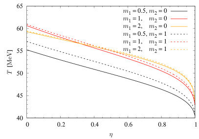
(a)

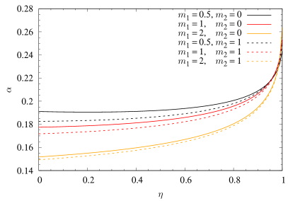
(b)

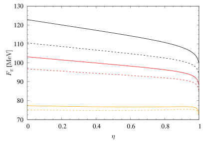
(c)

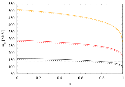
(d)

Figure 8: The (a) spin correction to the energy, (b) the dimensional coupling constant of the Skyrme and higher-order terms, (c) the pion decay constant and (d) the pion mass, all as functions of $\eta\in[0,1]$ which interpolates between the Skyrme model ($\eta=1$) and the higher-order model ($\eta=0$) $\mathcal{L}_{8a}$.

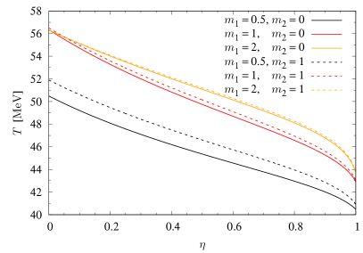
(a)

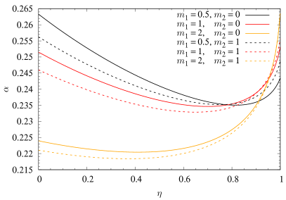
(b)

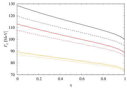
(c)

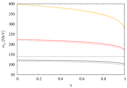
(d)

Figure 9: The (a) spin correction to the energy, (b) the dimensional coupling constant of the Skyrme and higher-order terms, (c) the pion decay constant and (d) the pion mass, all as functions of $\eta\in[0,1]$ which interpolates between the Skyrme model ($\eta=1$) and the higher-order model ($\eta=0$) $\mathcal{L}_{8b}$.

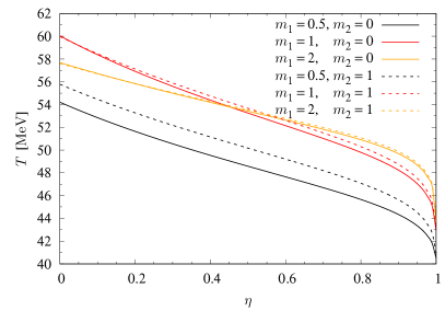
(a)

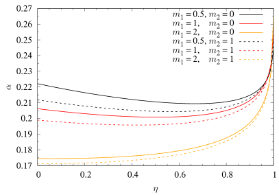
(b)

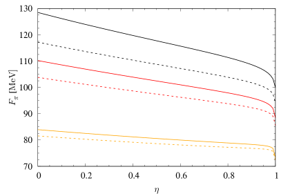
(c)

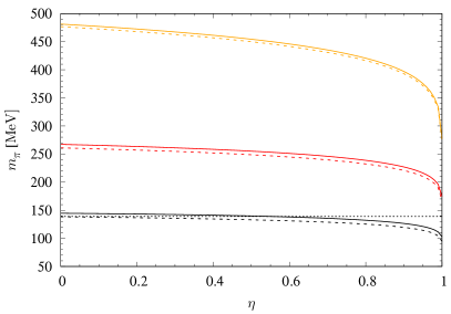
(d)

Figure 10: The (a) spin correction to the energy, (b) the dimensional coupling constant of the Skyrme and higher-order terms, (c) the pion decay constant and (d) the pion mass, all as functions of $\eta\in[0,1]$ which interpolates between the Skyrme model ($\eta=1$) and the higher-order model ($\eta=0$) $\mathcal{L}_{10}$.

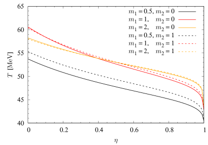
(a)

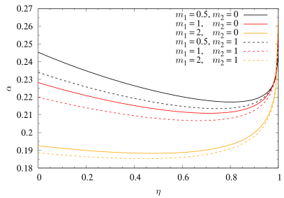
(b)

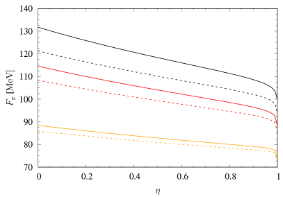
(c)

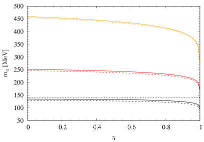
(d)

Figure 11: The (a) spin correction to the energy, (b) the dimensional coupling constant of the Skyrme and higher-order terms, (c) the pion decay constant and (d) the pion mass, all as functions of $\eta\in[0,1]$ which interpolates between the Skyrme model ($\eta=1$) and the higher-order model ($\eta=0$) $\mathcal{L}_{12}$.

We are now ready to present the numerical results for the higher-order Skyrme models (55)-(58), which are shown in Figs. 8-11. In the figures, the spin corrections to the energy is shown in panels (a), the dimensionless coupling constant $\alpha$ in panels (b), the pion decay constant in panels (c) and finally, the pion mass in panels (d). It is seen also for all the higher-order models, that the spin correction to the energy is smallest in the Skyrme model limit, i.e. for $\eta=1$.

IV Discussion and outlook

In this paper, we have studied the Skyrme model with the addition of the other possible fourth-order derivative term – the kinetic term squared, which however gives rise to more than two time derivatives in the model. Such model has been thought of as being impossible to quantize using rigid-body quantization, due to the presence of more than two time derivatives. We show in this work, however, that it is possible to perform rigid-body quantization in the case of the spherically symmetric $B=1$ hedgehog (the nucleon), since the equation that needs to be inverted in order to arrive at an expression in terms of the spin operator $J$ boils down to a cubic polynomial equation, that can be solved by Cardano’s well-known method.

We parametrized the model with a parameter $\eta$ that interpolates between the Skyrme model $(\eta=1)$, the pure kinetic term squared model $(\eta=1/2)$ and a new model with a negative Skyrme term that completely cancels off the kinetic term squared part $(\eta=0)$. Unfortunately, it turns out that the ambition of being able to reduce the spin contribution to the energy in this generalized fourth-order derivative version of the Skyrme model is not realizable. That is, the Skyrme model is the limit of this theory that has the smallest spin correction to the energy and hence mass of the Skyrmion. We have also analyzed a class of higher-order Skyrme models with four time derivatives and 8,10 and 12 derivatives in total. The quantization procedure carries over to this case by just recalculating the moments of inertia. Also in the case of all the four higher-order Skyrme models, the Skyrme model limit is the model with the lowest spin correction to the energy.

The result can have two opposite implications for future work on achieving physical binding energies. In one direction, one could go the BPS way and try to reduce the classical binding energies as well as the spin correction to the energy as much as possible. This is in the spirit of the assumption that the main contribution to the nucleon energy is the classical Skyrmion energy, and quantum corrections are small. If one chooses to go in another direction of acknowledging that the classical binding energies should not be small, but only the total binding energies must sum up to values that are at the percent level of the mass scale in question, then one could look at this extra degree of freedom of increasing the spin energy, if needed, as a tuning parameter. This latter approach to quantization of Skyrmions is discussed in Ref. [20] for the standard Skyrme model.

An issue with the current model, which we have not solved in this work, is to perform the quantization for Skyrmions that do not enjoy spherical symmetry. This becomes complicated because the moment of inertia tensor will no longer be proportional to the unit matrix; this implies that the cubic equation that we solve becomes a cubic matrix equation, that presumably is harder to solve. Common lore used to say that one cannot perform Hamiltonian quantization for the model with four or more time derivatives. We can now say that it is possible to perform rigid-body quantization if there is enough symmetry rendering the moment of inertia tensors proportional to the identity matrix (i.e. spherical symmetry or in principle translational symmetry). One may consider, as a first step, to solve the problem with axial symmetry, for which two eigenvalues of the tensors are equal. Nevertheless, if the complete model of quantization of Skyrmions requires the smallest possible spin contribution, then the Skyrme model is the best option, to the fourth order in the derivative expansion. We will leave for future work, a possible investigation of the spin contribution for non-spherically symmetric inertia tensors in this model or other models with more than two time derivatives. Although more complicated, we believe that the smallest root(s) of the cubic matrix equation can be found with numerical methods, if it is not possible to write down analytic expressions.

Another comment in store about theories with four or more time derivatives, is the problem of the Ostrogradsky instability [33]. In the formulation of Woodard [34], the dynamics of the Hamiltonian is generally described by two conjugate momenta, but only if the Lagrangian is nondegenerate in the double time derivative of some field. Luckily, although we have four time derivatives, they each act on their own field, making the theory highly nonlinear but not inducing the Ostrogradsky instability. One may wonder why there is no term like $\operatorname{tr}(U^{\dagger}\square U)^{2}$ in the most general Lagrangian of pions, but as shown in the literature such term can be eliminated by a field redefinition and it will be described at the four-derivative level just by the two terms included in the Lagrangian (5) plus higher-order terms in the derivative expansion [23, 24, 25, 26, 27]. The Ostrogradsky instability, which exists for nondegenerate double time derivatives, is due to the fact that the corresponding Hamiltonian will depend only linearly on one of the two conjugate momenta – this makes it possible to drive the theory into larger and larger energies with either sign. The theory thus has no lower or upper bound on the energy. In the case of the Ostrogradsky instability, arguments have been made that it is not an issue for EFTs, since the energy needed to excite a mode that possesses a run-away behavior is larger than the (cutoff) scale of the EFT and hence anyway beyond the validity of the EFT [35]. It has also been argued that in a certain class of asymptotically free theories, the effective mass of the unstable modes becomes infinitely heavy in the UV limit [36]. At some higher order in the derivative expansion, it will no longer be possible to eliminate all d’Alembertian operators from the EFT Lagrangian even using field redefinitions and integration-by-parts relations; at such order the Ostrogradsky instability is inevitable, although it is possible that it will not cause problems for the EFT observables at sufficiently small energies. Nevertheless, the Lagrangian (5) contains a term $-\operatorname{tr}(\partial_{t}U^{\dagger}\partial_{t}U)^{2}$, which for large time derivatives may also cause unwanted effects. In our treatment using rigid-body quantization, we do not encounter any problems with the theory possessing four time derivatives, but of course we have not treated the problem as a fully dynamical problem. We leave the scrutiny of possible dynamical instabilities for future work.

Finally, one may consider the possibility of going to a higher order in the derivative expansion, which has already been considered in the literature in the case of the theory containing only two time derivatives [37, 38, 9, 10, 39, 40]. Of course, one could also consider going to the sixth order in derivatives (or higher) and include all possible terms (up to field redefinitions and integration-by-parts relations), which however would give rise to a higher-order polynomial equation than the cubic equation studied in this paper. In particular, in the case of sixth-order derivative theories the corresponding order of the polynomial equation is of 5th order. For a $2n$-th order derivative theory, the corresponding polynomial equation for the squared spin operator would then be of order $2n-1$. In such cases, it is probably necessary to turn to numerical methods for finding the (smallest) roots. We leave such problems for future work.

Note added

After completion of this manuscript, it was brought to our attention that the model of Sec. II has been studied in the literature in Ref. [41] with which there is some overlap. To be precise, the model (5) is exactly the same as in Ref. [41] up to notation, but without a potential and hence without the pion mass, and the smallest root of the spin quantization has been calculated also in the latter reference; although we notice that Ref. [41] is missing a factor of 1/2 in the angle of their Eq. (4.12). The fact that the Skyrme model limit gives the smallest spin correction was not mentioned and the discussions of the two papers are completely different. In the updated version, we have extended this paper with the higher-order Skyrme models of Sec. III.

Acknowledgments

We thank Herbert Weigel for pointing out Ref. [41] to us. S. B. G. thanks Zhang Baiyang for discussions. S. B. G. thanks the Outstanding Talent Program of Henan University and the Ministry of Education of Henan Province for partial support. The work of S. B. G. is supported by the National Natural Science Foundation of China (Grants No. 11675223 and No. 12071111) and by the Ministry of Science and Technology of China (Grant No. G2022026021L).

Appendix A Positivity of static energy

In order to prove the entire suitable range of the couplings while retaining a positive definite static energy, we rewrite the derivative part of the static part of the Lagrangian (14) in terms of the 4-vector field $\mathbf{n}=(n^{0},n^{1},n^{2},n^{3})$:

$$U=n^{0}\mathbf{1}_{2}+\mathrm{i}\tau^{a}n^{a},\qquad a=1,2,3,$$ (85)

yielding

$$\mathcal{E} =(\partial_{i}\mathbf{n}\cdot\partial_{i}\mathbf{n})+\frac{2\eta-1}{2}(\partial_{i}\mathbf{n}\cdot\partial_{i}\mathbf{n})^{2}-\frac{2\eta-1}{2}(\partial_{i}\mathbf{n}\cdot\partial_{j}\mathbf{n})^{2}+\frac{1-\eta}{2}(\partial_{i}\mathbf{n}\cdot\partial_{i}\mathbf{n})^{2}.$$ (86)

Using the roots, $\{\lambda_{i}\}$, of the strain tensor [42]

$$D_{ij}=-\frac{1}{2}\operatorname{tr}[R_{i}R_{j}]=(\partial_{i}\mathbf{n}\cdot\partial_{j}\mathbf{n})=\left[V\begin{pmatrix}\lambda_{1}^{2}\\ &\lambda_{2}^{2}\\ &&\lambda_{3}^{2}\end{pmatrix}V^{\rm T}\right]_{ij},$$ (87)

we obtain

$$\mathcal{E}=(\lambda_{1}^{2}+\lambda_{2}^{2}+\lambda_{3}^{2})+\eta(\lambda_{1}^{2}\lambda_{2}^{2}+\lambda_{1}^{2}\lambda_{3}^{2}+\lambda_{2}^{2}\lambda_{3}^{2})+\frac{1-\eta}{2}(\lambda_{1}^{4}+\lambda_{2}^{4}+\lambda_{3}^{4}).$$ (88)

Clearly this (derivative part) of the static energy density is positive definite for $\eta\in[0,1]$.

References

- [1] T. H. R. Skyrme, A Nonlinear field theory, Proc. Roy. Soc. Lond. A 260 (1961) 127–138.
- [2] T. H. R. Skyrme, A Unified Field Theory of Mesons and Baryons, Nucl. Phys. 31 (1962) 556–569.
- [3] E. Witten, Global Aspects of Current Algebra, Nucl. Phys. B 223 (1983) 422–432.
- [4] E. Witten, Current Algebra, Baryons, and Quark Confinement, Nucl. Phys. B 223 (1983) 433–444.
- [5] G. S. Adkins, C. R. Nappi, and E. Witten, Static Properties of Nucleons in the Skyrme Model, Nucl. Phys. B 228 (1983) 552.
- [6] P. Sutcliffe, Skyrmions, instantons and holography, JHEP 08 (2010) 019, [arXiv:1003.0023].
- [7] P. Sutcliffe, Skyrmions in a truncated BPS theory, JHEP 04 (2011) 045, [arXiv:1101.2402].
- [8] M. F. Atiyah and N. S. Manton, Skyrmions From Instantons, Phys. Lett. B 222 (1989) 438–442.
- [9] C. Adam, J. Sanchez-Guillen, and A. Wereszczynski, A Skyrme-type proposal for baryonic matter, Phys. Lett. B 691 (2010) 105–110, [arXiv:1001.4544].
- [10] C. Adam, J. Sanchez-Guillen, and A. Wereszczynski, A BPS Skyrme model and baryons at large , Phys. Rev. D 82 (2010) 085015, [arXiv:1007.1567].
- [11] D. Harland, Topological energy bounds for the Skyrme and Faddeev models with massive pions, Phys. Lett. B 728 (2014) 518–523, [arXiv:1311.2403].
- [12] M. Gillard, D. Harland, and M. Speight, Skyrmions with low binding energies, Nucl. Phys. B 895 (2015) 272–287, [arXiv:1501.05455].
- [13] T. Sakai and S. Sugimoto, Low energy hadron physics in holographic QCD, Prog. Theor. Phys. 113 (2005) 843–882, [hep-th/0412141].
- [14] M. Harada and K. Yamawaki, Hidden local symmetry at loop: A New perspective of composite gauge boson and chiral phase transition, Phys. Rept. 381 (2003) 1–233, [hep-ph/0302103].
- [15] S. B. Gudnason, M. Barsanti, and S. Bolognesi, Near-BPS baby Skyrmions, JHEP 11 (2020) 062, [arXiv:2006.01726].
- [16] S. B. Gudnason, M. Barsanti, and S. Bolognesi, Near-BPS baby Skyrmions with Gaussian tails, JHEP 05 (2021) 134, [arXiv:2102.12134].
- [17] S. B. Gudnason, M. Barsanti, and S. Bolognesi, Near-BPS Skyrmions, JHEP 11 (2022) 092, [arXiv:2206.09559].
- [18] C. Adam, K. Oles, and A. Wereszczynski, The dielectric Skyrme model, Phys. Lett. B 807 (2020) 135560, [arXiv:2005.00018].
- [19] S. B. Gudnason, Dielectric Skyrmions, Phys. Rev. D 102 (2020), no. 11 116013, [arXiv:2009.03082].
- [20] S. B. Gudnason and C. Halcrow, Quantum binding energies in the Skyrme model, arXiv:2307.09272.
- [21] C. J. Houghton, N. S. Manton, and P. M. Sutcliffe, Rational maps, monopoles and Skyrmions, Nucl. Phys. B 510 (1998) 507–537, [hep-th/9705151].
- [22] R. A. Battye and P. M. Sutcliffe, Skyrmions, fullerenes and rational maps, Rev. Math. Phys. 14 (2002) 29–86, [hep-th/0103026].
- [23] J. Gasser and H. Leutwyler, Chiral Perturbation Theory to One Loop, Annals Phys. 158 (1984) 142.
- [24] J. Gasser and H. Leutwyler, Chiral Perturbation Theory: Expansions in the Mass of the Strange Quark, Nucl. Phys. B 250 (1985) 465–516.
- [25] H. W. Fearing and S. Scherer, Extension of the chiral perturbation theory meson Lagrangian to order p(6), Phys. Rev. D 53 (1996) 315–348, [hep-ph/9408346].
- [26] J. Bijnens, G. Colangelo, and G. Ecker, The Mesonic chiral Lagrangian of order p**6, JHEP 02 (1999) 020, [hep-ph/9902437].
- [27] J. Bijnens, S. B. Gudnason, J. Yu, and T. Zhang, Hilbert series and higher-order Lagrangians for the O(N) model, JHEP 05 (2023) 061, [arXiv:2212.07901].
- [28] G. S. Adkins and C. R. Nappi, The Skyrme Model with Pion Masses, Nucl. Phys. B 233 (1984) 109–115.
- [29] S. B. Gudnason, Loosening up the Skyrme model, Phys. Rev. D 93 (2016), no. 6 065048, [arXiv:1601.05024].
- [30] S. B. Gudnason and M. Nitta, Modifying the pion mass in the loosely bound Skyrme model, Phys. Rev. D 94 (2016), no. 6 065018, [arXiv:1606.02981].
- [31] S. B. Gudnason and C. Halcrow, Vibrational modes of Skyrmions, Phys. Rev. D 98 (2018), no. 12 125010, [arXiv:1811.00562].
- [32] S. B. Gudnason and M. Nitta, A higher-order Skyrme model, JHEP 09 (2017) 028, [arXiv:1705.03438].
- [33] M. Ostrogradsky, Mémoires sur les équations différentielles, relatives au problème des isopérimètres, Mem. Acad. St. Petersbourg 6 (1850), no. 4 385–517.
- [34] R. P. Woodard, Ostrogradsky’s theorem on Hamiltonian instability, Scholarpedia 10 (2015), no. 8 32243, [arXiv:1506.02210].
- [35] A. R. Solomon and M. Trodden, Higher-derivative operators and effective field theory for general scalar-tensor theories, JCAP 02 (2018) 031, [arXiv:1709.09695].
- [36] M. Asorey, F. Falceto, and L. Rachwał, Asymptotic freedom and higher derivative gauge theories, JHEP 05 (2021) 075, [arXiv:2012.15693].
- [37] G. S. Adkins and C. R. Nappi, Stabilization of Chiral Solitons via Vector Mesons, Phys. Lett. B 137 (1984) 251–256.
- [38] A. Jackson, A. D. Jackson, A. S. Goldhaber, G. E. Brown, and L. C. Castillejo, A MODIFIED SKYRMION, Phys. Lett. B 154 (1985) 101–106.
- [39] S. B. Gudnason, B. Zhang, and N. Ma, Generalized Skyrme model with the loosely bound potential, Phys. Rev. D 94 (2016), no. 12 125004, [arXiv:1609.01591].
- [40] S. B. Gudnason, Exploring the generalized loosely bound Skyrme model, Phys. Rev. D 98 (2018), no. 9 096018, [arXiv:1805.10898].
- [41] D. E. L. Pottinger and E. Rathske, Metastability of Solitons in a Generalized Skyrme Model, Phys. Rev. D 33 (1986) 2448.
- [42] N. S. Manton, Geometry of Skyrmions, Commun. Math. Phys. 111 (1987) 469.