OmniSeg3D: Omniversal 3D Segmentation via
Hierarchical Contrastive Learning

Abstract

Towards holistic understanding of 3D scenes, a general 3D segmentation method is needed that can segment diverse objects without restrictions on object quantity or categories, while also reflecting the inherent hierarchical structure. To achieve this, we propose OmniSeg3D, an omniversal segmentation method aims for segmenting anything in 3D all at once. The key insight is to lift multi-view inconsistent 2D segmentations into a consistent 3D feature field through a hierarchical contrastive learning framework, which is accomplished by two steps. Firstly, we design a novel hierarchical representation based on category-agnostic 2D segmentations to model the multi-level relationship among pixels. Secondly, image features rendered from the 3D feature field are clustered at different levels, which can be further drawn closer or pushed apart according to the hierarchical relationship between different levels. In tackling the challenges posed by inconsistent 2D segmentations, this framework yields a global consistent 3D feature field, which further enables hierarchical segmentation, multi-object selection, and global discretization. Extensive experiments demonstrate the effectiveness of our method on high-quality 3D segmentation and accurate hierarchical structure understanding. A graphical user interface further facilitates flexible interaction for omniversal 3D segmentation.

1 Introduction

3D segmentation forms one of the cornerstones in 3D scene understanding, which is also the basis of 3D interaction, editing, and extensive applications in virtual reality, medical analysis, and robot navigation. To meet the requirement of complex world sensing, a general/omniversal category-agnostic 3D scene segmentation method is required, capable of segmenting any object in 3D without limitations on object quantity or categories. For instance, to accurately discretize a pavilion as shown in Fig. 1, the user needs to accurately segment each roof, column, eaves, and other intricate structures. Existing 3D-based segmentation methods based on 3D point clouds, meshes, or volumes fall short of these requirements. They are either restricted to limited categories due to the scarcity of large-scale 3D datasets, such as learning-based methods [15, 26, 21], or they only identify local geometric similarity or smoothness without extracting semantic information, as typified by traditional algorithms [38, 17, 12].

An alternative approach involves lifting 2D image understanding to 3D space, leveraging the impressive class-agnostic 2D segmentation performance achieved by recent methods [22, 24, 7, 27, 40]. Current lifting-based methods either rely on annotated 2D masks [53, 3, 45], or are restricted to a limited set of pre-defined classes [39, 2]. Other methods propose distilling semantic-rich image features [36, 24] onto point clouds [35, 42] or NeRF [20, 23, 14]. However, due to the absence of boundary information, directly distilling these semantic feature into 3D space often leads to noisy segmentations [35, 20]. Further works use SAM [22] or video segmentation methods [31] to generate accurate 2D masks of targeted objects, and unproject them into 3D space [5]. However, these approaches are limited to single-object segmentation and exhibit unstable results in cases with severe occlusion because the 2D segmentation is performed on each image independently.

Therefore, significant challenges still persist. First, multi-view consistency remains an obstacle due to the substantial variations in 2D segmentations across different viewpoints. Second, ambiguity arises when distinguishing in-the-wild objects like eaves and roofs, which inherently possess a hierarchical semantic structure. To this end, we propose OmniSeg3D, an Omniversal 3D Segmentation method which enjoys multi-object, category-agnostic, and hierarchical segmentation in 3D all at once. We demonstrate that a global 3D feature field (which can be formulated on point cloud, mesh, NeRF [30], etc) is inherently well-suited for integrating occlusion-free, boundary-clear, and hierarchical semantic information from 2D segmentations through hierarchical contrastive learning. The key lies in hierarchically clustering 2D image features rendered from the 3D feature field at different levels of segmentation blocks, where the multi-level segmentations are specified by a proposed hierarchical 2D representation. Then the clustered features will be drawn closer or pushed apart via a hierarchical contrastive loss, which enables the learning of a feature field that encodes hierarchical information into the proximity of feature distances, effectively eliminating semantic inconsistencies between different images. This unified framework facilitates multi-object selection, hierarchical segmentation, global discretization, and a broad range of applications.

We evaluate OmniSeg3D on segmentation tasks for single object selection and hierarchical inference. Extensive quantitative and qualitative results on real-world and synthetic datasets demonstrate our method enjoys high-quality 3D object segmentation and holistic comprehension of scene structure across various scales. An interactive interface is also provided for flexible 3D segmentation. Our contributions are summarized as follows:

• We propose a hierarchical 2D representation to reveal and store the part-level relationship within objects based on class-agnostic 2D segmentations and a voting strategy.

• We present a hierarchical contrastive learning method to optimize a globally consistent 3D hierarchical feature field given 2D observations.

• Extensive experiments demonstrate that our omniversal 3D segmentation framework can segment anything in 3D all at once, which enables hierarchical segmentation, multi-object selection, and 3D discretization.

2 Related Works

2.1 2D Segmentation

2D segmentation has experienced a long history. Early works mainly rely on the clue of pixel similarity and continuity [13, 11, 1] to segment images. Since the introduction of FCN [29], there has been a rapid expansion in research of different sub-fields of 2D segmentation [16, 21, 6, 51]. The involvement of transformer [43] in the segmentation domain has led to the proposal of several novel segmentation architectures [52, 9, 10]. However, most of these methods are limited to pre-defined class labels.

Prompt-based segmentation is a special task that enables segmenting unseen object categories [27, 7, 40]. One recent breakthrough is the Segment Anything Model (SAM) [22], aiming to unify the 2D segmentation task through the introduction of a prompt-based segmentation approach , is considered a promising innovation in the field of vision.

2.2 3D Segmentation

Closed-set segmentation. The task of 3D segmentation has been explored with various types of 3D representation such as RGBD images [44, 46], pointcloud [48, 47, 18], and voxels [19, 28, 15, 26]. However, due to the insufficiency of annotated 3D datasets for training a unified 3D segmentation model, they are still limited to closed-set 3D understanding, which largely restrict the application scenarios.

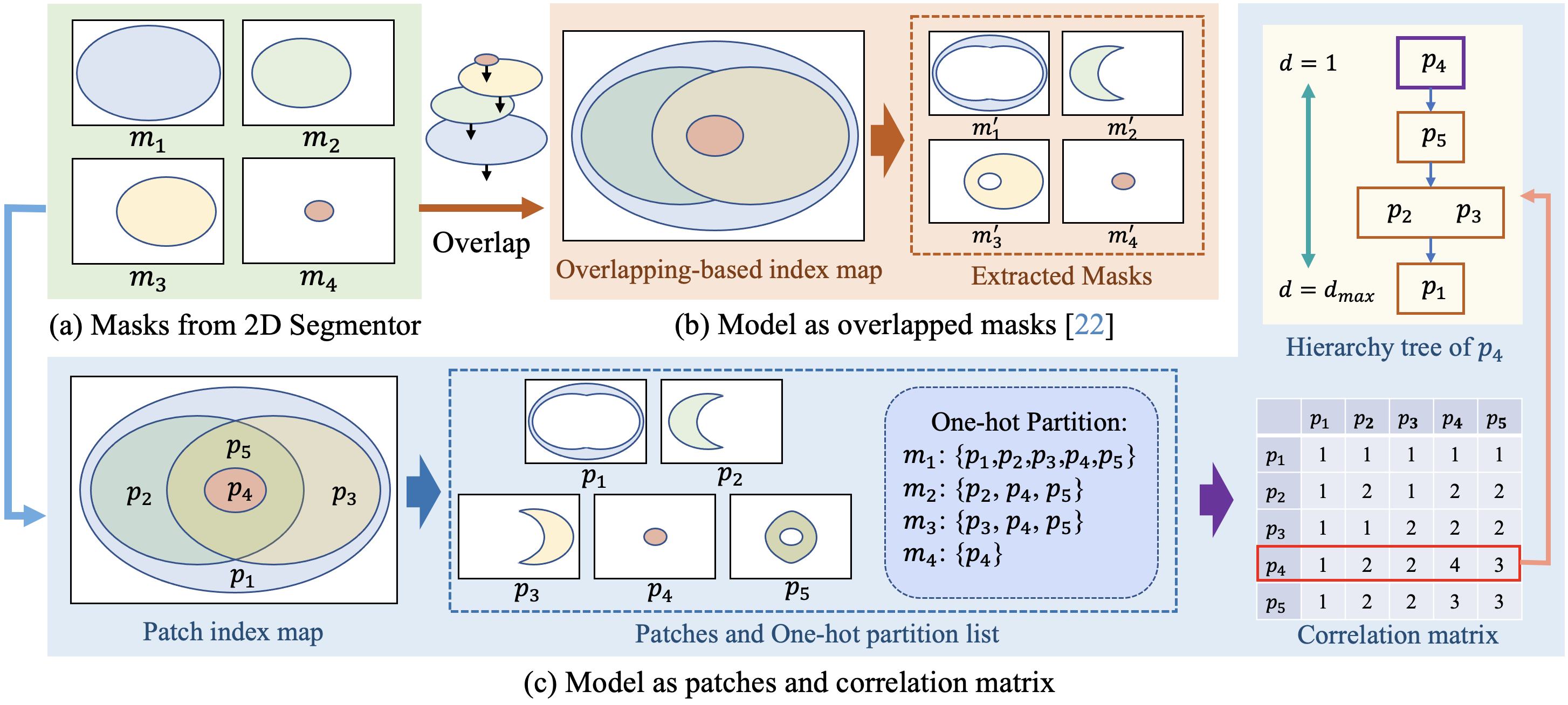
Figure 2: Illustration of our proposed hierarchical representation. (a) For each image, click-based 2D segmentors provide a set of masks $\{m_{i}\}$. (b) Directly overlapping masks implemented by conventional methods [22] lead to the loss of hierarchical information. (c) Patch-based modeling effectively preserves inclusion information. The hierarchical representation of each image includes a patch index map $I_{p}$ and a correlation matrix $C_{hi}$, where the relevance between $p_{i}$ and other patches is evaluated via a voting strategy.

Given the shortage of 3D datasets essential for the development of foundational 3D models, recent works have proposed to lift 2D information into 3D for 3D segmentation and understanding. Some works rely on ground truth masks [53, 3, 45] or pre-trained 2D semantic/instance segmentation models for mask generation [39, 2]. However, ground truth annotation is unrealistic for general cases, and model-based methods typically only offer closed-set object masks. ContrastiveLift [2] proposes to segment closed-set 3D objects via contrastive learning. However, it cannot handle unseen classes and reveal object hierarchy. In contrast, our method achieves panoptic, category-agnostic, and hierarchical segmentation based on a hierarchical contrastive learning framework, which can be interpreted as a sound combination of click-based segmentation methods and holistic 3D modeling.

Open-set segmentation. LERF [20] and subsequent works [14, 23, 42] propose to distill language feature [36] into 3D space for open-vocabulary interactive segmentation. Since the learned feature is trained on entire images without explicit boundary supervision, these methods prone to produce noisy segmentation boundaries. Besides, these methods are unable to distinguish different instances due to the lack of instance-level supervision. Alternatively, we take advantage of category-agnostic segmentation methods and distill the 2D results into 3D to get a consistent feature field and enable high-quality 3D segmentation.

SPInNeRF [31] utilizes video segmentation to initialize 2D masks and then lift them into 3D space with a NeRF. A followed multi-view refinement stage is utilized to achieve consistent 3D segmentation. SA3D [5] introduces an online interactive segmentation method that propagates one SAM [22] mask into 3D space and other views iteratively. However, these methods may heavily rely on a good choice of reference view and cannot handle complex cases such as severe occlusion. Instead, our method can segment anything in 3D all at once via a global consistent feature field, which is more robust to object occlusion.

Hierarchical segmentation. For hierarchical segmentation, existing methods mainly focus on category-specific scenario [33, 32] or geometric analysis [8, 49, 48], which are not suitable for general hierarchical 3D segmentation. Instead, we propose to distill hierarchical information from 2D into 3D space to achieve multi-view consistent hierarchical segmentation in 3D.

3 Methods

Given a set of calibrated input images and the corresponding 2D segmentation masks, our goal is to learn a 3D feature field that enjoys multi-object, category-agnostic, and hierarchical segmentation all at once. We first segment 2D images into smaller units $P_{segs}$ and construct our novel hierarchical 2D representation. Then we hierarchically cluster 2D image features $\mathbf{f}\in\mathbb{R}^{D}$ rendered from the 3D feature field at different levels of patches $P_{segs}$, which will further be supervised to construct correct feature distance order between sampled points via the proposed hierarchical contrastive clustering strategy. In this section, we first introduce the representation in Sec. 3.1, which includes both basic and hierarchical implementation for lifting inconsistent 2D masks into 3D space. Then, a hierarchical contrastive learning method for optimizing the 3D feature field will be discussed (Sec. 3.2). Finally, the applications for various interactive segmentation will be introduced.

3.1 Hierarchical Representation

Preliminary: Class-agnostic 2D segmentation. To achieve omniversal segmentation, a 2D segmentation method should be able to handle unseen categories. We seek solution from click-based method like SAM [22], which exhibits a class-agnostic property. Given an input image $I$, a grid of points (typically $32\times 32$) are sampled as the input prompts to generate a set of 2D binary masks $M_{segs}=\{m_{i}\in\mathbb{R}^{H\times W}|i=1,...,|M_{segs}|\}$ as proposals (see Fig. 2(a)). To get a label map as training data for 3D field optimization (like in [53]), masks in $M_{segs}$ are overlapped one by one according to the number of contained pixels in the masks in [22] (see Fig. 2(b)). Since each pixel in image $I$ may belong to more than one masks in $M_{segs}$ (consider the fact that a pixel belonging to the mask of a chair may also belong to the mask of the chair’s leg), directly overlapping masks, as done in SAM, may destroy the rich hierarchical information embedded inside $M_{segs}$.

Hierarchical Modeling. To avoid the aforementioned problem, we design a novel representation that preserves the hierarchical information within each image. Specifically, instead of using overlapped masks, we divide the entire 2D image into disjoint patches. As shown in Fig. 2(a), let $m_{i}\in M_{segs},(i=1,...,4)$ represent masks in $M_{segs}$. For each pixel, we create a one-hot vector to indicate which masks the pixel belongs to. To eliminate the impact of overlapping, we define the patch set $P_{segs}$ as the smallest collection of pixels that share the same one-hot vector. These patches can also be interpreted as the smallest units in the image that are exhaustively partitioned by $M_{segs}$ (as shown in Fig. 2(c)). This also results in a patch index map $I_{p}$, where each pixel contains a index of the patch.

Next, we proceed to model the hierarchical structure with patches $P_{segs}$ as the unit and the original masks $M_{segs}$ as the correlation binding. The core idea is that, if two patches fall into the same mask, then these two patches has some degree of correlation. To model the strength of the correlation, we introduce a voting-based rating strategy. Specifically, for each pair of patches $p_{i}$ and $p_{j}$, we count the number of masks that contain both $p_{i}$ and $p_{j}$. By traversing all the patch pairs, we get a matrix $C_{hi}\in\mathbb{R}^{N_{p}\times N_{p}}$:

$$C_{hi}(p_{i},p_{j})=\sum_{k=1}^{N_{m}}\mathbbm{1}(p_{i}\subseteq m_{k})\cdot\mathbbm{1}(p_{j}\subseteq m_{k}),$$ (1)

where $N_{m}=|M_{segs}|$ represents the number of masks and $N_{p}=|P_{segs}|$ represents the number of patches. $N_{p}$ typically ranges from $200$ to $500$ in our experiments. This process can be interpreted as utilizing masks to vote for the relationship between patches. To deduce the hierarchical relationship between patches, we select a patch $p_{i}$ as the anchor and take the $i$-th row of matrix $C_{hi}(p_{i},\cdot)=v_{i}$. We then sort the patches according to the vote counts in vector $v_{i}$ and construct a hierarchical tree for anchor patch $p_{i}$, as illustrated in Fig. 2(c). Patches located at shallower depths in the tree has stronger relevance to the anchor patch $p_{i}$, which can be taken as the guidance of the hierarchical contrastive learning introduced in the subsequent section. Finally, the hierarchical representation for each image consists of a patch index map $I_{p}$ and a correlation matrix $C_{hi}$.

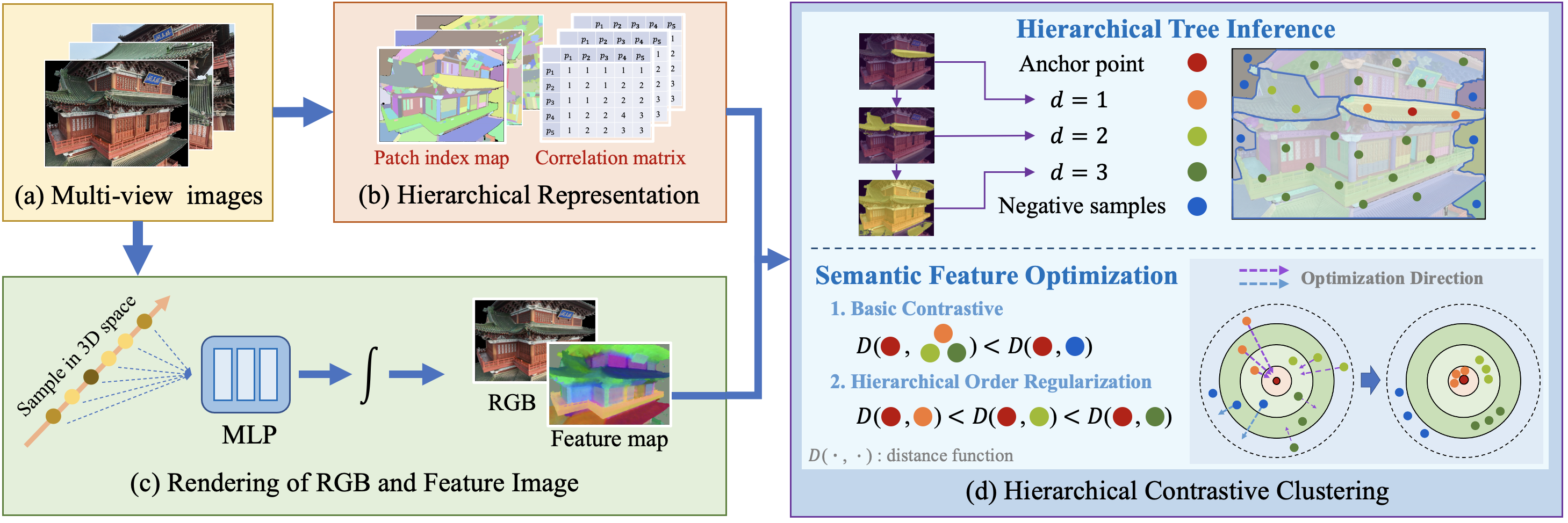
Figure 3: Framework of hierarchical contrastive learning. (a) For each input RGB image, we apply (b) 2D hierarchical modeling to get a patch index map and a correlation matrix. During training, we utilize (c) NeRF-based rendering pipeline to render features from 3D space and apply hierarchical contrastive learning (d) to the rendered features to optimize the feature field for segmentation.

3.2 Hierarchical Contrastive Learning

In this section, we show how to lift the hierarchical relationship of 2D patches into the 3D space through hierarchical contrastive learning.

3D feature field. We start by introducing a 3D feature field that establishes the relationship between 2D images and the 3D space. This feature field is based on NeRF-like rendering methods [30, 34]. Specifically, for each point $\mathbf{x}_{i}\in\mathbb{R}^{3}$ in the 3D space, we define a segmentation identity feature $\mathbf{f_{i}}\in\mathbb{R}^{D}$. Along the view direction $\mathbf{d}_{i}\in\mathbb{R}^{2}$, an MLP network $F_{\mathbf{\Theta}}$ generates per-point attributes:

$$(\sigma_{i},\mathbf{f}_{i})=F_{\mathbf{\Theta}}(\gamma_{1}(\mathbf{x}_{i})),\ \ \ \mathbf{c}_{i}=F_{\mathbf{\Theta}}(\gamma_{1}(\mathbf{x}_{i}),\gamma_{2}(\mathbf{d}_{i})),$$ (2)

where $\gamma_{1}$ and $\gamma_{2}$ are positional encoding functions in [34].

Subsequently, color and density are integrated along the ray to generate the rendered pixel color $\mathbf{c}(\mathbf{r})$:

$$\mathbf{c}(\mathbf{r})=\sum_{i=1}^{N}T_{i}\alpha_{i}\mathbf{c}_{i},\ \ \ T_{i}=\prod_{j=1}^{i-1}(1-\alpha_{i}),$$ (3)

where $\alpha_{i}=1-exp(-\sigma_{i}\delta_{i})$ is the opacity and $\delta_{i}=r_{i+1}-r_{i}$ is the distance between adjacent samples. Besides, feature maps can be rendered as:

$$\mathbf{f}(\mathbf{r})=\sum_{i=1}^{N}T_{i}\alpha_{i}\mathbf{f}_{i}.$$ (4)

Basic implementation. In this section, we present a basic implementation of our approach that lifts 2D segmentations into 3D space without considering hierarchical information.

The core idea is to apply contrastive learning to lift 2D category-agnostic segmentation to 3D. For each image, we randomly sample $N$ points on it and identify the patch id each point belongs to. Then we render features $\{\mathbf{f_{i}}\}(i\in[1,N])$ of these points via differentiable rendering from the 3D feature field. For each sampled point, we designate points with the same patch id as positive samples, and all the other sampled points as negative ones. The correlation between two 3D points is modelled as the cosine distance $\mathbf{f}_{i}\cdot\mathbf{f}_{j}$.

To accelerate the loss calculation and get stable convergence, we apply the contrastive clustering method [25]. Specifically, we define cluster $\{\mathbf{f}^{i}\}$ as the collection of rendered features that share the same patch id $i$. The center of each cluster is defined as the mean value $\bar{\mathbf{f}}^{i}$ of features in $\{\mathbf{f}^{i}\}$. Then for each chosen feature point $\mathbf{f}^{i}_{j}$ with patch id $i$ and point index $j$ within cluster $\{\mathbf{f}^{i}\}$, both positive samples and negative samples are replaced with the mean feature $\bar{\mathbf{f}}^{i}$ and $\bar{\mathbf{f}}^{k}$. The loss is shown below, which favors high similarity between $\mathbf{f}^{i}_{j}$ and $\bar{\mathbf{f}}^{i}$ that belongs to the same cluster and low similarity between $\mathbf{f}^{i}_{j}$ and $\bar{\mathbf{f}}^{k}$:

$$\mathcal{L}_{CC}=-\frac{1}{N_{p}}\sum_{i=1}^{N_{p}}\sum_{j=1}^{|\{\mathbf{f}^{i}\}|}\log{\frac{\exp(\mathbf{f}^{i}_{j}\cdot\bar{\mathbf{f}}^{i}/\phi_{i})}{\sum_{k=1}^{N_{p}}\exp(\mathbf{f}^{i}_{j}\cdot\bar{\mathbf{f}}^{k}/\phi_{k})}},$$ (5)

where $N_{p}$ is the number of patch ids, $\phi_{i}$ is the temperature of cluster $i$ to balance the cluster size and variance: $\phi_{i}={\sum_{j=1}^{n_{i}}||\mathbf{f}^{i}_{j}-\bar{\mathbf{f}}^{i}||_{2}}/{n_{i}\log(n_{i}+\alpha)},\ \ n_{i}=|\{\mathbf{f}^{i}\}|$. $\alpha=10$ is a smoothing parameter to prevent small clusters from exhibiting an excessively large $\phi_{i}$.

Note that ConstrastiveLift [2] uses a slow-fast learning strategy for stable training. We refer to contrastive clustering [25] to realize faster training and stable convergence.

Hierarchical implementation. Here we show how to incorporate hierarchical information into the pipeline of contrastive learning. We first cluster the sampled point features ${\mathbf{f}}$ into feature point sets $\{\mathbf{f}^{i}\},(i\in[1,N_{p}])$ based on the 2D image patches. Then for each anchor patch ${p_{i}}$, we assign all related patches with their depths in the hierarchy tree $d\in[1,d^{i}_{max}]$ according to the correlation matrix $C_{hi}$. Note that all the related patches are potential positive samples in this formulation.

To achieve hierarchical contrastive clustering in 3D, we employ the hierarchical regularization proposed in [50]. Firstly, we add a regularization term $\lambda^{d-1}$ to Eq. 5 with a per-level decay factor $\lambda\leq 1$, which means higher penalty are applied to the patches with stronger correlations to the anchor patch $i$. Secondly, a regularization of the optimization order is implemented to ensure that a patch higher in the hierarchy tree (smaller $d$) exhibits a higher feature similarity with the anchor patch than patches at lower levels (as shown in Fig. 3(d)). The final loss is shown below:

$$\mathcal{L}_{H}=\sum_{i=1}^{N_{p}}\sum_{d=1}^{d^{i}_{max}}\frac{\lambda^{d-1}}{NL}\sum_{j=1}^{|\{\mathbf{f}^{i}\}|}\sum_{s\in S_{d}^{i}}\max(\mathcal{L}^{i,j}(s),\mathcal{L}_{max}^{i,j}(d-1)),$$ (6)

where $S^{i}_{d}$ is the patch index set at level $d$ of anchor patch $i$ (For example, $S_{d=3}^{i=4}=\{2,3\}$ in Fig. 2), $s\in S^{i}_{d}$ is a patch at depth $d$, $\mathcal{L}^{i,j}(s)$ is the contrastive loss between point $j$ (in point set of patch $i$) and the average feature $\bar{\mathbf{f}}^{s}$ of patch $s$:

$$\mathcal{L}^{i,j}(s)=-\log{\frac{\exp(\mathbf{f}^{i}_{j}\cdot\bar{\mathbf{f}}^{s}/\phi_{s})}{\sum_{k=1}^{N_{p}}\exp(\mathbf{f}^{i}_{j}\cdot\bar{\mathbf{f}}^{k}/\phi_{k})}},$$ (7)

and $\mathcal{L}_{max}^{i,j}(d)$ is the maximum loss at level $d$:

$$\mathcal{L}_{max}^{i,j}(d)=\max_{s\in S^{i}_{d}}\mathcal{L}^{i,j}(s).$$ (8)

Since the volumetric rendering may introduce ambiguity in the calculation of the integration, we found that it is better to apply normalization loss to regularize the feature vector and ensure it distributed on the sphere surface:

$$\mathcal{L}_{norm}=\frac{1}{N}\sum_{i=1}^{N}\left({||\mathbf{f}_{i}||-1}\right)^{2}.$$ (9)

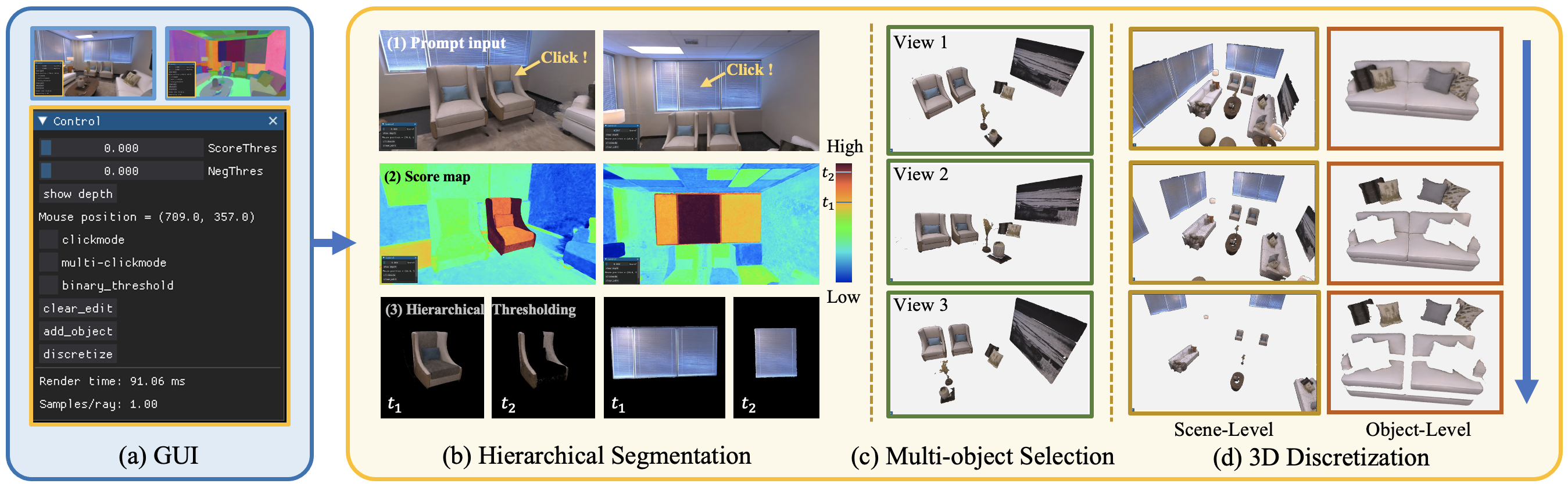
Figure 4: Interactive 3D segmentation with (a) a graphical user interface. For room-0 of Replica, we show the segmentation performance on (b) hierarchical inference, (c) multi-object selection, and (d) 3D discretization with our GUI.

3.3 Implementation details

During training, we optimize the MLP $F_{\mathbf{\Theta}}$ and the semantic feature volume $\mathbf{V_{s}}$ (with feature dimension $D=16$) via volume rendering, where four loss functions are applied: $\mathcal{L}_{c}=\sum_{\mathbf{r}}\left\|\mathbf{c}(\mathbf{r})-\mathbf{c}_{\mathrm{gt}}(\mathbf{r})\right\|^{2}_{2}$, $\mathcal{L}_{reg}=\sum_{\mathbf{r}}-o(\mathbf{r})\log(o(\mathbf{r}))$, where $o(\mathbf{r})=\sum_{i=1}^{N}T_{i}\alpha_{i}$ is the opacity of each ray. $\mathcal{L}_{reg}$ is used to regularize each ray to be completely saturated or empty. The per-level decay factor is set to $\lambda=0.5$. The total loss is:

$$\mathcal{L}_{total}=\mathcal{L}_{c}+w_{1}\mathcal{L}_{H}+w_{2}\mathcal{L}_{norm}+w_{3}\mathcal{L}_{reg}$$ (10)

The hyper-parameters are set to $w_{1}=5\times 10^{-4},w_{2}=5\times 10^{2},w_{3}=1\times 10^{-3}$ for all the experiments. With a cosine annealing schedule, the learning rate is set from $1\times 10^{-2}$ to $3\times 10^{-4}$. The number of rays in each batch is 8192. We train our model for 50000 iterations for each scene.

The proposed omniversal segmentation scheme can be seen as a lightweight plug-in which can be easily integrated into reconstruction methods based on common 3D representations like NeRF, mesh, and point cloud. For 2D backbones, though we use SAM [22] in our implementation, any click-based segmentation methods like  [40, 27, 7] can be used as a substitute. Please refer to our supplementary material for more details.

3.4 Interactive Segmentation

To realize flexible and interactive 3D segmentation, we develop a graphical user interface (GUI). This GUI can serve as a novel 3D annotation tool, which may largely improve the efficiency of 3D data annotation. Two typical cases based on NeRF and mesh are shown in Fig. 4 and Fig. 1.

With a single click on the object of interest, our model generates a score field based on feature similarities. By adjusting the binarization threshold, the segmentation can seamlessly traverse the scene hierarchy from atomic components to entire objects, and holistic portions of the scene. Besides, users can select and segment multiple objects simultaneously through multiple clicks. Based on the input clicks, a region-growing approach is employed to segment the mesh and extract discrete components, which can be saved as 3D assets.

4 Experiments

4.1 Hierarchical 3D Segmentation

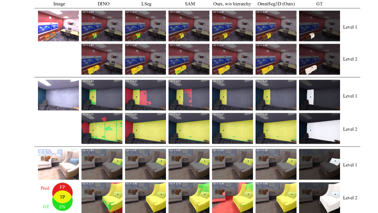
Figure 5: Comparison of hierarchical segmentation results on the Replica dataset. Prompts are shown as black dots. Colored pixels denote TP: True-Positive, FP: False-Positive and FN: False-Negative respectively.

Dataset.

To quantitatively evaluate our OmniSeg3D, we set up a scene-scale dataset with hierarchical semantic annotations. We utilize the Replica dataset [41] processed by Semantic-NeRF [53], which comprises 8 realistic indoor scenes. We uniformly sample a total of 281 images and manually annotated each image with a query pixel $\mathbf{q}$ and two corresponding masks, the smaller one $M_{L_{1}}$ properly included by the larger one $M_{L_{2}}\supset M_{L_{1}}$. $M_{L_{1}}$ and $M_{L_{2}}$ typically correspond to object parts and complete instances respectively, as shown in Fig. 5. In case multiple levels of reasonable segmentations $M_{a}\subset M_{b}\subset M_{c}$ exist, we choose different pairs as the ground truth $(M_{L_{1}},M_{L_{2}})$ in different images, so that the selected masks exhibit diverse scales and represent the full range of possible hierarchical relationships present in the scene.

Benchmark.

We benchmark our algorithm as follows. The model receives as input a 2D query point $\mathbf{q}$ in the given frame $\mathbf{I}$, and is expected to output a dense 2D score map $\{\mathrm{score}\,(\mathbf{p})\,|\,\mathbf{p}\in\mathbf{I}\}$. Ideally, there exist thresholds ${th}_{1}>{th}_{2}$ which, when applied to the score map, yields $M_{L_{1}}\subset M_{L_{2}}$ respectively:

$$\exists\,{th}_{i}\,\,s.t.\,\,M_{L_{i}}=\{\mathbf{p}\in\mathbf{I}\,|\,\mathrm{score}\,(\mathbf{p})>{th}_{i}\}.$$ (11)

For evaluation, we choose the thresholds $({th}_{1},{th}_{2})$ that maximize the IoU between the predicted masks and the ground truth $(M_{L_{1}},M_{L_{2}})$, and define the metrics as:

$$\begin{aligned} \mathrm{IoU}_{L_{i}}&=\max_{{th}_{i}}{\mathrm{IoU}\,(\{\mathbf{p}\in\mathbf{I}\,|\,\mathrm{score}\,(\mathbf{p})>{th}_{i}\},M_{L_{i}})},\\ \mathrm{IoU}_{Avg}&=(\mathrm{IoU}_{L_{1}}+\mathrm{IoU}_{L_{2}})/2.\end{aligned}$$ (12)

Method	mIoU (%)
	Level 1	Level 2	Average
DINO [4]	67.9	64.2	66.1
LSeg [24]	51.7	82.1	66.9
SAM [22]	92.8	80.2	86.5
Ours, w/o hierarchy	93.1	80.4	86.7
OmniSeg3D (ours)	91.3	88.9	90.1

Table 1: Comparison of hierarchical segmentation on Replica [41].

Baseline methods.

We first compare our OmniSeg3D with state-of-the-art 2D segmentation models and semantic feature extractors. SAM [22] predicts three hierarchical masks from the point query. We compare each to the ground truth masks $(M_{L_{1}},M_{L_{2}})$ and report the highest IoU. DINO [4] and LSeg [24] (based on CLIP [36]) predict a feature image, which is converted to a score map based on cosine similarities and then binarized using Eq. 12 to compute the IoU. In addition, we compare our full method with the basic implementation in Sec. 3.2, i.e., 3D contrastive learning without hierarchical modelling.

Results.

Tab. 1 demonstrates the quantitative results of hierarchical segmentation on the Replica [41] dataset. Fig. 5 shows the qualitative results. Our OmniSeg3D achieves the highest average mIoU, while substantially leading in level-2 segmentation, which features high-level semantics.

As shown in Fig. 5, the self-supervised DINO method struggles to delineate clear object boundaries. LSeg captures overall semantics better but fails to discriminate between instances. SAM performs well at fine-grained segmentation, but occasionally fails to group together multiple objects or large regions, resulting in lower level-2 mIoU. Our basic implementation without hierarchical modeling inherits these characteristics of SAM, with slightly better metrics. Our full method degrades in level-1 segmentation due to the shifted emphasis on the omniversal task, while achieving large improvements in high-level segmentation. This implies that the hierarchical modelling effectively aggregates fragmented part-whole correlations from multiple views. We hypothesize that the 3D contrastive learning implicitly aggregates and averages the voting-based correlations from multi-view inputs, distilling a stable hierarchical semantic order into the 3D representation, thereby enhancing global-scale semantic clustering.

4.2 3D Instance Segmentation

While designed for omniversal 3D segmentation, our method is able to handle 3D instance segmentation as a sub-task. Different from existing methods [31, 5], OmniSeg3D does not require instance-specific training. The 3D feature field is trained only once for each scene and reused for different instances, while still performing competitively on datasets proposed by previous work.

We follow NVOS [37], SPIn-NeRF [31] and SA3D [5] to benchmark 3D instance segmentation as prompt propagation. For each scene, given prompts (scribbles or masks) in the reference view, the algorithm is supposed to segment the instance in the target view. The predicted mask is compared with the ground truth target view segmentation. As shown in Tab. 2, OmniSeg3D outperforms the baseline methods in terms of mIoU and pixel-wise classification accuracy, while alleviating the need to retrain different segmentation fields for the same scene.

Dataset	Method	mIoU (%)	Acc (%)
NVOS	NVOS [37]	70.1	92.0
	ISRF [14]	83.8	96.4
	SA3D [5]	90.3	98.2
	OmniSeg3D (ours)	91.7	98.4
MVSeg	MVSeg [31]	93.3	98.7
	SA3D [5]	92.8	98.7
	OmniSeg3D (ours)	95.2	99.2
Replica	MVSeg [31]	32.4	-
	SA3D [5]	83.0	-
	OmniSeg3D (ours)	84.4	-

Table 2: Quantitative comparison of instance segmentation.

4.3 Ablation Studies

Hierarchical decay.

As illustrated in Eq. 6, we apply a decay $\lambda\in[0,1]$ to downweight the contrastive loss for patches of lower correlation with the anchor. Setting $\lambda=0$ resembles the basic implementation without hierarchical modeling, while setting $\lambda=1$ puts equal emphasis on samples from all hierarchies, enhancing high-level semantics. Tab. 3 demonstrates hierarchical segmentation results on the Replica dataset. With the increase of $\lambda$, $\mathrm{IoU}_{L_{1}}$ decreases while $\mathrm{IoU}_{L_{2}}$ increases, reaching $\mathrm{IoU}_{L_{1}}\approx\mathrm{IoU}_{L_{2}}$ at $\lambda=1$. We choose $\lambda=0.5$ with the highest average mIoU, implying a balance between local and global semantic clustering. For instance segmentation, the influence of $\lambda$ on mIoU is counteracted when averaged on instances with various sizes and containing different levels of hierarchies.

Hierar.	Per-level	Hierar. mIoU (%)			Instance
model	decay $\lambda$	Lv.1	Lv.2	Avg.	mIoU (%)
$\times$	-	93.1	80.4	86.7	83.6
✓	0.1	92.5	84.7	88.6	84.3
✓	0.2	92.1	86.5	89.4	84.6
✓	0.5	91.3	88.9	90.1	84.4
✓	1	89.2	89.2	89.2	83.3

Table 3: Ablation of hierarchical modelling on Replica.

Feature dimension.

We study how the dimension $D$ of semantic features affects the performance of hierarchical contrastive clustering. As shown in Tab. 4, the average mIoU first increases with $D$, then nearly saturates beyond $D=16$. Therefore, we assume $D=16$ is sufficient for our algorithm.

Feat. dim.	4	8	16	32	64	128
Avg. mIoU	89.8	91.8	93.0	93.0	93.1	93.2

Table 4: Ablation of feature dimensions on room-0 of Replica.

5 Limitations

Figure 6: Scene discretization by feature clustering on mesh automatically without click.

Due to the absence of a clear definition for hierarchy levels, there is no assurance that the objects will be segmented at the same level by simply clustering features (see Fig. 6). To address this issue, text-aligned hierarchical segmentation may be a future direction. Besides, since the contrastive learning is applied on single images, two objects that have never appeared in the same image may have similar semantic feature. This problem can be alleviated by introducing local geometric continuity, but global contrastive learning across images is also a topic worth exploring.

6 Conclusion

In this paper, we propose OmniSeg3D, an omniversal segmentation method that facilitates holistic understanding of 3D scenes. Leveraging a hierarchical representation and a hierarchical contrastive learning framework, OmniSeg3D effectively transforms inconsistent 2D segmentations into a globally consistent 3D feature field while retaining hierarchical information, which enables correct hierarchical 3D sensing and high-quality object segmentation performance. Besides, variant interactive functionalities including hierarchical inference, multi-object selection, and global discretization are realized, which may further enable downstream applications in the field of 3D data annotation, robotics and virtual reality.

References

- Achanta et al. [2012] Radhakrishna Achanta, Appu Shaji, Kevin Smith, Aurelien Lucchi, Pascal Fua, and Sabine Süsstrunk. Slic superpixels compared to state-of-the-art superpixel methods. IEEE transactions on pattern analysis and machine intelligence, 34(11):2274–2282, 2012.
- Bhalgat et al. [2023] Yash Bhalgat, Iro Laina, João F Henriques, Andrew Zisserman, and Andrea Vedaldi. Contrastive lift: 3d object instance segmentation by slow-fast contrastive fusion. arXiv preprint arXiv:2306.04633, 2023.
- Bing et al. [2022] WANG Bing, Lu Chen, and Bo Yang. Dm-nerf: 3d scene geometry decomposition and manipulation from 2d images. In The Eleventh International Conference on Learning Representations, 2022.
- Caron et al. [2021] Mathilde Caron, Hugo Touvron, Ishan Misra, Hervé Jégou, Julien Mairal, Piotr Bojanowski, and Armand Joulin. Emerging properties in self-supervised vision transformers. In Proceedings of the International Conference on Computer Vision (ICCV), 2021.
- Cen et al. [2023] Jiazhong Cen, Zanwei Zhou, Jiemin Fang, Wei Shen, Lingxi Xie, Xiaopeng Zhang, and Qi Tian. Segment anything in 3d with nerfs. arXiv preprint arXiv:2304.12308, 2023.
- Chen et al. [2017] Liang-Chieh Chen, George Papandreou, Iasonas Kokkinos, Kevin Murphy, and Alan L Yuille. Deeplab: Semantic image segmentation with deep convolutional nets, atrous convolution, and fully connected crfs. IEEE transactions on pattern analysis and machine intelligence, 40(4):834–848, 2017.
- Chen et al. [2022] Xi Chen, Zhiyan Zhao, Yilei Zhang, Manni Duan, Donglian Qi, and Hengshuang Zhao. Focalclick: Towards practical interactive image segmentation. In Proceedings of the IEEE/CVF Conference on Computer Vision and Pattern Recognition, pages 1300–1309, 2022.
- Chen et al. [2020] Zhiqin Chen, Andrea Tagliasacchi, and Hao Zhang. Bsp-net: Generating compact meshes via binary space partitioning. In Proceedings of the IEEE/CVF Conference on Computer Vision and Pattern Recognition, pages 45–54, 2020.
- Cheng et al. [2021] Bowen Cheng, Alex Schwing, and Alexander Kirillov. Per-pixel classification is not all you need for semantic segmentation. Advances in Neural Information Processing Systems, 34:17864–17875, 2021.
- Cheng et al. [2022] Bowen Cheng, Ishan Misra, Alexander G Schwing, Alexander Kirillov, and Rohit Girdhar. Masked-attention mask transformer for universal image segmentation. In Proceedings of the IEEE/CVF conference on computer vision and pattern recognition, pages 1290–1299, 2022.
- Coleman and Andrews [1979] Guy Barrett Coleman and Harry C Andrews. Image segmentation by clustering. Proceedings of the IEEE, 67(5):773–785, 1979.
- Dorninger and Nothegger [2007] Peter Dorninger and Clemens Nothegger. 3d segmentation of unstructured point clouds for building modelling. International Archives of the Photogrammetry, Remote Sensing and Spatial Information Sciences, 35(3/W49A):191–196, 2007.
- Felzenszwalb and Huttenlocher [2004] Pedro F Felzenszwalb and Daniel P Huttenlocher. Efficient graph-based image segmentation. International journal of computer vision, 59:167–181, 2004.
- Goel et al. [2023] Rahul Goel, Dhawal Sirikonda, Saurabh Saini, and PJ Narayanan. Interactive segmentation of radiance fields. In Proceedings of the IEEE/CVF Conference on Computer Vision and Pattern Recognition, pages 4201–4211, 2023.
- Han et al. [2020] Lei Han, Tian Zheng, Lan Xu, and Lu Fang. Occuseg: Occupancy-aware 3d instance segmentation. In Proceedings of the IEEE/CVF conference on computer vision and pattern recognition, pages 2940–2949, 2020.
- He et al. [2017] Kaiming He, Georgia Gkioxari, Piotr Dollár, and Ross Girshick. Mask r-cnn. In Proceedings of the IEEE international conference on computer vision, pages 2961–2969, 2017.
- Höhne and Hanson [1992] Karl Heinz Höhne and William A Hanson. Interactive 3d segmentation of mri and ct volumes using morphological operations. Journal of computer assisted tomography, 16(2):285–294, 1992.
- Hu et al. [2020] Qingyong Hu, Bo Yang, Linhai Xie, Stefano Rosa, Yulan Guo, Zhihua Wang, Niki Trigoni, and Andrew Markham. Randla-net: Efficient semantic segmentation of large-scale point clouds. In Proceedings of the IEEE/CVF conference on computer vision and pattern recognition, pages 11108–11117, 2020.
- Huang and You [2016] Jing Huang and Suya You. Point cloud labeling using 3d convolutional neural network. In 2016 23rd International Conference on Pattern Recognition (ICPR), pages 2670–2675. IEEE, 2016.
- Kerr et al. [2023] Justin Kerr, Chung Min Kim, Ken Goldberg, Angjoo Kanazawa, and Matthew Tancik. Lerf: Language embedded radiance fields. In Proceedings of the IEEE/CVF International Conference on Computer Vision, pages 19729–19739, 2023.
- Kirillov et al. [2019] Alexander Kirillov, Kaiming He, Ross Girshick, Carsten Rother, and Piotr Dollár. Panoptic segmentation. In Proceedings of the IEEE/CVF conference on computer vision and pattern recognition, pages 9404–9413, 2019.
- Kirillov et al. [2023] Alexander Kirillov, Eric Mintun, Nikhila Ravi, Hanzi Mao, Chloe Rolland, Laura Gustafson, Tete Xiao, Spencer Whitehead, Alexander C Berg, Wan-Yen Lo, et al. Segment anything. arXiv preprint arXiv:2304.02643, 2023.
- Kobayashi et al. [2022] Sosuke Kobayashi, Eiichi Matsumoto, and Vincent Sitzmann. Decomposing nerf for editing via feature field distillation. Advances in Neural Information Processing Systems, 35:23311–23330, 2022.
- Li et al. [2022] Boyi Li, Kilian Q Weinberger, Serge Belongie, Vladlen Koltun, and Rene Ranftl. Language-driven semantic segmentation. In International Conference on Learning Representations, 2022.
- Li et al. [2020] Junnan Li, Pan Zhou, Caiming Xiong, and Steven Hoi. Prototypical contrastive learning of unsupervised representations. In International Conference on Learning Representations, 2020.
- Liu et al. [2022] Leyao Liu, Tian Zheng, Yun-Jou Lin, Kai Ni, and Lu Fang. Ins-conv: Incremental sparse convolution for online 3d segmentation. In Proceedings of the IEEE/CVF Conference on Computer Vision and Pattern Recognition, pages 18975–18984, 2022.
- Liu et al. [2023] Qin Liu, Zhenlin Xu, Gedas Bertasius, and Marc Niethammer. Simpleclick: Interactive image segmentation with simple vision transformers. In Proceedings of the IEEE/CVF International Conference on Computer Vision, pages 22290–22300, 2023.
- Liu et al. [2019] Zhijian Liu, Haotian Tang, Yujun Lin, and Song Han. Point-voxel cnn for efficient 3d deep learning. Advances in Neural Information Processing Systems, 32, 2019.
- Long et al. [2015] Jonathan Long, Evan Shelhamer, and Trevor Darrell. Fully convolutional networks for semantic segmentation. In Proceedings of the IEEE conference on computer vision and pattern recognition, pages 3431–3440, 2015.
- Mildenhall et al. [2021] Ben Mildenhall, Pratul P Srinivasan, Matthew Tancik, Jonathan T Barron, Ravi Ramamoorthi, and Ren Ng. Nerf: Representing scenes as neural radiance fields for view synthesis. Communications of the ACM, 65(1):99–106, 2021.
- Mirzaei et al. [2023] Ashkan Mirzaei, Tristan Aumentado-Armstrong, Konstantinos G Derpanis, Jonathan Kelly, Marcus A Brubaker, Igor Gilitschenski, and Alex Levinshtein. Spin-nerf: Multiview segmentation and perceptual inpainting with neural radiance fields. In Proceedings of the IEEE/CVF Conference on Computer Vision and Pattern Recognition, pages 20669–20679, 2023.
- Mo et al. [2019a] Kaichun Mo, Paul Guerrero, Li Yi, Hao Su, Peter Wonka, Niloy Mitra, and Leonidas J Guibas. Structurenet: Hierarchical graph networks for 3d shape generation. arXiv preprint arXiv:1908.00575, 2019a.
- Mo et al. [2019b] Kaichun Mo, Shilin Zhu, Angel X Chang, Li Yi, Subarna Tripathi, Leonidas J Guibas, and Hao Su. Partnet: A large-scale benchmark for fine-grained and hierarchical part-level 3d object understanding. In Proceedings of the IEEE/CVF conference on computer vision and pattern recognition, pages 909–918, 2019b.
- Müller et al. [2022] Thomas Müller, Alex Evans, Christoph Schied, and Alexander Keller. Instant neural graphics primitives with a multiresolution hash encoding. ACM Transactions on Graphics (ToG), 41(4):1–15, 2022.
- Peng et al. [2023] Songyou Peng, Kyle Genova, Chiyu Jiang, Andrea Tagliasacchi, Marc Pollefeys, Thomas Funkhouser, et al. Openscene: 3d scene understanding with open vocabularies. In Proceedings of the IEEE/CVF Conference on Computer Vision and Pattern Recognition, pages 815–824, 2023.
- Radford et al. [2021] Alec Radford, Jong Wook Kim, Chris Hallacy, Aditya Ramesh, Gabriel Goh, Sandhini Agarwal, Girish Sastry, Amanda Askell, Pamela Mishkin, Jack Clark, et al. Learning transferable visual models from natural language supervision. In International conference on machine learning, pages 8748–8763. PMLR, 2021.
- Ren et al. [2022] Zhongzheng Ren, Aseem Agarwala, Bryan Russell, Alexander G Schwing, and Oliver Wang. Neural volumetric object selection. In Proceedings of the IEEE/CVF Conference on Computer Vision and Pattern Recognition, pages 6133–6142, 2022.
- Schnabel et al. [2007] Ruwen Schnabel, Roland Wahl, and Reinhard Klein. Efficient ransac for point-cloud shape detection. In Computer graphics forum, pages 214–226. Wiley Online Library, 2007.
- Siddiqui et al. [2023] Yawar Siddiqui, Lorenzo Porzi, Samuel Rota Bulò, Norman Müller, Matthias Nießner, Angela Dai, and Peter Kontschieder. Panoptic lifting for 3d scene understanding with neural fields. In Proceedings of the IEEE/CVF Conference on Computer Vision and Pattern Recognition, pages 9043–9052, 2023.
- Sofiiuk et al. [2022] Konstantin Sofiiuk, Ilya A Petrov, and Anton Konushin. Reviving iterative training with mask guidance for interactive segmentation. In 2022 IEEE International Conference on Image Processing (ICIP), pages 3141–3145. IEEE, 2022.
- Straub et al. [2019] Julian Straub, Thomas Whelan, Lingni Ma, Yufan Chen, Erik Wijmans, Simon Green, Jakob J. Engel, Raul Mur-Artal, Carl Ren, Shobhit Verma, Anton Clarkson, Mingfei Yan, Brian Budge, Yajie Yan, Xiaqing Pan, June Yon, Yuyang Zou, Kimberly Leon, Nigel Carter, Jesus Briales, Tyler Gillingham, Elias Mueggler, Luis Pesqueira, Manolis Savva, Dhruv Batra, Hauke M. Strasdat, Renzo De Nardi, Michael Goesele, Steven Lovegrove, and Richard Newcombe. The Replica dataset: A digital replica of indoor spaces. arXiv preprint arXiv:1906.05797, 2019.
- Takmaz et al. [2023] Ayça Takmaz, Elisabetta Fedele, Robert W Sumner, Marc Pollefeys, Federico Tombari, and Francis Engelmann. Openmask3d: Open-vocabulary 3d instance segmentation. arXiv preprint arXiv:2306.13631, 2023.
- Vaswani et al. [2017] Ashish Vaswani, Noam Shazeer, Niki Parmar, Jakob Uszkoreit, Llion Jones, Aidan N Gomez, Łukasz Kaiser, and Illia Polosukhin. Attention is all you need. Advances in neural information processing systems, 30, 2017.
- Wang and Neumann [2018] Weiyue Wang and Ulrich Neumann. Depth-aware cnn for rgb-d segmentation. In Proceedings of the European conference on computer vision (ECCV), pages 135–150, 2018.
- Wu et al. [2022] Qianyi Wu, Xian Liu, Yuedong Chen, Kejie Li, Chuanxia Zheng, Jianfei Cai, and Jianmin Zheng. Object-compositional neural implicit surfaces. In European Conference on Computer Vision, pages 197–213. Springer, 2022.
- Xing et al. [2020] Yajie Xing, Jingbo Wang, and Gang Zeng. Malleable 2.5 d convolution: Learning receptive fields along the depth-axis for rgb-d scene parsing. In European Conference on Computer Vision, pages 555–571. Springer, 2020.
- Yang et al. [2019] Bo Yang, Jianan Wang, Ronald Clark, Qingyong Hu, Sen Wang, Andrew Markham, and Niki Trigoni. Learning object bounding boxes for 3d instance segmentation on point clouds. Advances in neural information processing systems, 32, 2019.
- Yi et al. [2019] Li Yi, Wang Zhao, He Wang, Minhyuk Sung, and Leonidas J Guibas. Gspn: Generative shape proposal network for 3d instance segmentation in point cloud. In Proceedings of the IEEE/CVF Conference on Computer Vision and Pattern Recognition, pages 3947–3956, 2019.
- Yu et al. [2022] Fenggen Yu, Zhiqin Chen, Manyi Li, Aditya Sanghi, Hooman Shayani, Ali Mahdavi-Amiri, and Hao Zhang. Capri-net: Learning compact cad shapes with adaptive primitive assembly. In Proceedings of the IEEE/CVF Conference on Computer Vision and Pattern Recognition, pages 11768–11778, 2022.
- Zhang et al. [2022] Shu Zhang, Ran Xu, Caiming Xiong, and Chetan Ramaiah. Use all the labels: A hierarchical multi-label contrastive learning framework. In Proceedings of the IEEE/CVF Conference on Computer Vision and Pattern Recognition, pages 16660–16669, 2022.
- Zhao et al. [2017] Hengshuang Zhao, Jianping Shi, Xiaojuan Qi, Xiaogang Wang, and Jiaya Jia. Pyramid scene parsing network. In Proceedings of the IEEE conference on computer vision and pattern recognition, pages 2881–2890, 2017.
- Zheng et al. [2021] Sixiao Zheng, Jiachen Lu, Hengshuang Zhao, Xiatian Zhu, Zekun Luo, Yabiao Wang, Yanwei Fu, Jianfeng Feng, Tao Xiang, Philip HS Torr, et al. Rethinking semantic segmentation from a sequence-to-sequence perspective with transformers. In Proceedings of the IEEE/CVF conference on computer vision and pattern recognition, pages 6881–6890, 2021.
- Zhi et al. [2021] Shuaifeng Zhi, Tristan Laidlow, Stefan Leutenegger, and Andrew J Davison. In-place scene labelling and understanding with implicit scene representation. In Proceedings of the IEEE/CVF International Conference on Computer Vision, pages 15838–15847, 2021.