CurriculumLoc: Enhancing Cross-Domain Geolocalization through Multi-Stage Refinement

Abstract

Visual geolocalization is a cost-effective and scalable task that involves matching one or more query images, taken at some unknown location, to a set of geo-tagged reference images. Existing methods, devoted to semantic features representation, evolving towards robustness to a wide variety between query and reference, including illumination and viewpoint changes, as well as scale and seasonal variations. However, practical visual geolocalization approaches need to be robust in appearance changing and extreme viewpoint variation conditions, while providing accurate global location estimates. Therefore, inspired by curriculum design, human learn general knowledge first and then delve into professional expertise. We first recognize semantic scene and then measure geometric structure. Our approach, termed CurriculumLoc, involves a delicate design of multi-stage refinement pipeline and a novel keypoint detection and description with global semantic awareness and local geometric verification. We rerank candidates and solve a particular cross-domain perspective-n-point (PnP) problem based on these keypoints and corresponding descriptors, position refinement occurs incrementally. The extensive experimental results on our collected dataset, TerraTrack and a benchmark dataset, ALTO, demonstrate that our approach results in the aforementioned desirable characteristics of a practical visual geolocalization solution. Additionally, we achieve new high recall@1 scores of 62.6% and 94.5% on ALTO, with two different distances metrics, respectively. Dataset, code and trained models are publicly available on https://github.com/npupilab/CurriculumLoc.

I Introduction

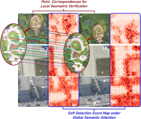
Figure 1: Visualization of pixel correspondences supervision and soft detection score of matched images during training. White represents low soft-detection scores while red signifies higher ones. The training lowers the soft-detection scores on repetitive structures (e.g. ground, floor, walls) while it enhances the score on more distinctive points. And during training soft detection scores are optimized under the supervision of pixel correspondences.

A high quality, view aware image often captures sufficient information to uniquely represent a location [34] . Meanwhile, it is convenient to capture aerial images, with low cost and high adaptability camera. Therefore, it is not surprising that we use vision as the primary source of information for UAVs localization, navigation, and exploration in remote sensing.

Currently, vision-based localization is tackled either with structure-based methods, such as Structure-from-Motion (SfM) [1, 2, 3, 4] and Simultaneous Localization and Mapping (SLAM) [5, 6, 7, 8], or with retrieval-based approaches [9, 10, 11, 12, 13]. Structure-based methods estimate relative poses based on precise 3D-2D point correspondences, which can only output relative positions rather than geolocations, and the estimation error will increase with the accumulation of distance [14]. The application of geolocalization in remote sensing is limited primarily because of the high computational demand [15]. This limitation is usually alleviated using additional sensory systems such as Global Positioning System (GPS) and landmarks [16]. However, the loss of GPS signal is inevitable due to various unpredictable factors in real-world flight missions. Furthermore, most existing structure-based methods focus on the accurate local descriptions of individual keypoints, which neglect their relationships established from global awareness [17, 18]. It’s easy to generate mismatches due to appearance changes such as lighting, viewpoint, and weather, and even cause positioning failures, especially in cross-domain tasks. There is a well-known trade-off between discriminative power and invariance for local descriptors [14].

Retrieval-based geolocalization is an appealing alternative that estimates the location where a given photo was taken by comparing it with a large database of geo-tagged reference images. Recent developments in learning image features for object detection and semantic segmentation have made image retrieval a viable method for localization [19, 20, 21, 22]. Its main goal is to design high-level semantic feature representation algorithms that are invariant to both appearance (year, season, and illumination) and viewpoint (translation and rotation) changes in the always changing world, like human instinct [23]. However, due to the lack of geometric transformation, retrieval-based geolocalization cannot provide accurate pose and associated location. Moreover, it needs to deal with additional challenges in remote sensing, primarily stemming from the domain disparities between the query UAV images and the reference satellite images.

In this work, we rethink the visual geolocalization problem from the lens of robust human perception and precise geometry measurement. We first adopt a general retrieval approach to obtain the top-$k$ candidates of the reference database, which are the nearest neighbors to the current aerial image in the semantic space of global representations. These global descriptors represents the invariant features related to locations, initial retrieval in this feature space helps to ignore the interference of appearance changes such as lighting, season, weather, etc. on localization robustness.

Besides, we introduce a novel symmetric Swin Transformer with skip connections and shift window attention for keypoints descriptors construction called Swin-Descriptors. The motivation is to use the attention in Swin Transformer to enhance nonlocal awareness, thereby enhancing the invariance to appearance changes at the same location. Furthermore, to enhance the acquisition of salient and consistent keypoints and their corresponding descriptors representations, we devise a soft detection score to detect keypoints, which is derived from transformer extracted dense feature and is optimized by an extend ranking loss with point geometric verification. Our experiments show that descriptors construct from our Swin-Descriptors are promising in addressing the trade-off between discriminative power and invariance of local descriptors.

Besides, we rerank the initial candidates through the stereo matching relationships based on these keypoint descriptors, which significantly enhances the retrieval performance, particularly in terms of recall@1 and recall@5. Moreover, by utilizing the discriminative power and invariance of these keypoints descriptors, we formulate a cross-domain PnP problem between the query UAV image and the corresponding candidate geotagged satellite images. We show that solving this PnP problem yields a more accurate geolocation estimate than the geotag obtained from reranked recall@1.

In summary, our main contributions are:

• We propose a new pipeline of visual geolocalization called CurriculumLoc, which measuring the cross-domain geometric co-visibility structure after obtaining a coarse location through an incremental retrieval, resulting in robustness and desirable accuracy of a practical visual geolocalization solution.

• By leveraging a novel symmetric hierarchical transformer with attention mechanism during dense feature extraction, and a soft detection score for keypoint detection derive from dense feature under pixel correspondences supervision, the keypoint undergo comprehensive exposure to both global contextual awareness and local geometric verification during the training process, as illustrated in Fig. 1.

• To evaluate the effectiveness of CurriculumLoc, we create a publicly available dataset containing sequences of UAV and satellite imagery captured under challenging conditions for cross-domain geolocalization, named TerraTrack.

II Related Work

In this section, we discuss the recent researches that utilize structure-based methods or retrieval-based methods for visual localization and transformer architecture for vision tasks.

II-A Structure-based visual localization

Existing structure-based localization works can broadly divided into: (i) Structure-from-Motion (SfM); (ii) Simultaneous Localization and Mapping (SLAM). Both of these, when not augmented with additional sensors, are capable of obtaining only relative position information. Specifically, SfM is primarily employed for offline detailed reconstruction, while SLAM focuses on real-time localization and mapping. Both rely heavily on precise relative pose estimation, which are greatly dependent on the quality of keypoint detection and description.

In early localization systems [24, 25], conventional techniques like SIFT [26], SURF [27] and ORB [28] were extensively employed to characterize a small patch centered on a detected keypoint. However, it’s evident that these manually designed features with out global semantic attention struggle with significant appearance variations. More recently, CNN-based methods have demonstrated superior performance. Some of these approaches have suggested a two-stage process where keypoints are initially detected based on local structures and subsequently described using a separate CNN [29, 30]. Notably, LIFT [31] and LFNet [29] present distinct two-stage algorithms for keypoint detection and patch description based on the detected keypoints. In contrast to the aforementioned two-stage methods, certain approaches advocate for a unified one-stage approach for keypoint detection and description. SuperPoint [17], for instance, employs a self-supervised framework with a bootstrap training strategy to concurrently train a model for keypoint detection and descriptor extraction. On the other hand, R2D2 [32] incorporates effective loss functions to assess both the repeatability and reliability of keypoints detection. Furthermore, DomainFeat [22] enhances the extraction of robust descriptors and the detection of accurate keypoints by leveraging domain adaptation to learn local features.

Different from these prior works, we recommend the introduction of non-local awareness to include both hierarchical feature extraction with shift window attention mechanism and geometric verification, aiming to make the keypoints descriptors remarkable (easy to extract), invariant (not varying with rotation, translation, scaling and illumination changes) and accurate (accurate to measure).

II-B Retrieval-based visual localization

II-B1 Global Descriptors

Traditional global descriptors are usually obtained by aggregating local descriptors, such as Bag of Words (BoW), Fisher Kernal, and Vector of Locally Aggregated Descriptors (VLAD), have been used to assign visual words to images. Since the remarkable results of the NetVLAD [9] algorithm based on contrastive learning and adopting CNNs, researchers have been focusing on how to extract accurate and robust global descriptors to achieve retrieval localization.

Recent advances in global representation for retrieval cover a wide range of techniques and strategies. These include ranking loss-based learning [33], soft contrastive learning [34], innovative pooling methods [35], contextual feature reweighting [36], large-scale retraining [37], semantic-guided feature aggregation [38], 3D information integration[39], incorporation of additional sensors like event camera [40], sequence information [41], graph representation [42] and training with classification proxy [42, 43].

Distinct from these retrieval methods only focuses on global representation of images, we argue that global descriptors are suitable for robust scene recognition to determine a rough location range, while exact location requires geometric motion model from accurate local correspondences.

II-B2 Local Region/Patch Descriptors

In addition to global retrieval methods, some researchers have also been dedicated to learning task-specific patch-level features for place recognition. Patch-NetVLAD [10] demonstrates that this two-stage retrieval strategy, global retrieval and then rerank based on local features correlation verification, can improve the accuracy of place recognition. Patch-NetVLAD [10] exploit patch-level features from pretrained NetVLAD [9] residuals. Distinct from Patch-NetVLAD only considering aggregating local features, TransVLAD [12] design a attention-based feature extraction network with a sparse transformer, which both improves global contextual reasoning and aggregates a discriminative and compact global descriptor.

Furthermore, we design an Encoder-Decoder hierarchical transformer, Swin-Descriptors, to detect and describe keypoints. We fully leverage the geometric relationship between matched points to obtain more accurate rerank top-1, and return the final precise position by solving the camera motion model of UAV, rather than return the closest satellite image geo-tag.

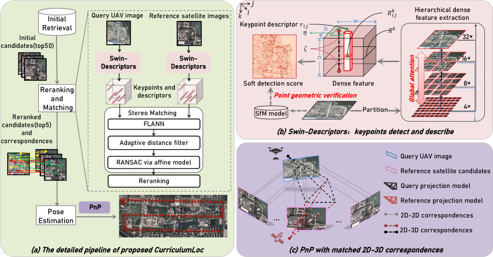
Figure 2: (a): The detailed pipeline of proposed CurriculumLoc. (b): Details of Swin-Descriptors in (a). (c): The schematic of cross-domian PnP in (a).

II-C Attention for visual localization

Attention mechanism, inspired by the human visual and cognitive systems, has been successfully employed applied to the learning of image-level global descriptors [44, 45, 12] for image retrieval tasks. In these methods, the attention is used as the weight of local descriptors, and global descriptors are derived from local descriptors through weighted summation. Directly applying these descriptors lead to poor results due to the lack of supervision of local pixel correspondence [32]. Attention mechanisms in these methods are optimized with the supervision of image-level, and it is not suitable for the pixel correspondence supervision. Moreover, existing attention mechanisms designed for location-based image retrieval is encouraged to focus on the most representative regions of the image rather than identifying suitable regions to maintain the location consistency and detecting invariant points for geometric matching.

In contrast, we propose a novel soft detection score for attention computing and feature extraction to improve the keypoint geometric consistency and matching accuracy. On the one hand, our soft detection score can find remarkable points for matching (easily detect to inliers while distinguishable to outliers) through a SfM model supervision. On the other hand, our soft detection enforces the same response for the matched points between different domain query and reference images, so it can provide extra priors to improve the robustness in matching process under changes in the appearance of the same location. Meanwhile, we leverage the shift window attention in Swin Transformer for our symmetric transformer to maintain scale invariance.

III Methodology

Our approach begins by utilizing global semantic feature to obtain the top-$k$ candidates (where $k$=50) that are most likely to represent the same location as the given query image. Following this, we employ a novel keypoint descriptor construction method called Swin-Descriptors to detect and describe keypoints in both query image and the top-$50$ candidates. Simultaneously, we rerank these reference images, and return the selection of the top-$5$ candidates along with their corresponding matched keypoint pairs. In the end, by computing the PnP using matched keypoint pairs between the top-$5$ candidates and the current UAV image, we can recover the camera motion model of UAV, ultimately achieving a more accurate localization than relying solely on the geotag of the nearest satellite in the reference database.

This multi-stage approach enhances geolocalization accuracy and robustness while minimizing the additional computational cost associated with keypoint matching and PnP solving. An overview of the complete pipeline can be found in Fig. 2(a).

III-A Initial Retrieval

We use a lightweight VGG-16 [46] network cropped at the last convolutional layer and extend it with a NetVLAD [9] layer as implemented by [10], initializing the network with off-the-shelf ImageNet [47] classification weights, and retaining the first few layers of weights for general feature extraction. Specifically, given an query image $\mathcal{q}$, outputs a $H\times W\times D$ dimensional features into a $K\times D$ dimensional matrix by summing the residuals between each feature $x_{i}\in\mathbb{R}^{D}$ and $K$ learned cluster centers weighted by soft-assignment. Formally, for $N\times D$ dimensional features, let the global aggregation layer $f_{global}:\mathbb{R}^{N\times D}\rightarrow\mathbb{R}^{K\times D}$ be given by

$$f_{global}(F)(j,k)=\sum_{i=1}^{N}\bar{a}_{k}(X_{i})(x_{i}(j)-c_{k}(j)),$$ (1)

where $x_{i}(j)$ is the $j^{th}$ element of the $i_{th}$ descriptor, $\bar{a}_{k}$ is the soft-assignment function and $c_{k}$ denotes the $k^{th}$ cluster center. After aggregation, the resultant matrix is then projected down into a dimensionality reduced vector using a projection layer $f_{proj}:\mathbb{R}^{K\times D}\rightarrow\mathbb{R}^{D_{proj}}$ by first applying intra (column) wise normalization, unrolling into a single vector, L2-normalizing in its entirety and finally applying PCA (learned on a training set) with whitening and L2-normalization. Refer to [9] for more details.

We use this global feature for initial retrieval and return top-$50$ reference satellite images. This step helps us quickly retrieve satellite images from a database that are geographically close to the query UAV image’s location, primarily based on feature distance, even though it may contain erroneous matches. Subsequently, reordering is performed based on geometric verification through local point matching, which enhances accuracy while saving time.

III-B Swin-Descriptors

Contrary to existing two-stage methods, which rerank global retrieval results by local semantic feature verification, such as PatchNetVLAD [10], we propose to preform dense semantic feature extraction to obtain a local representation that is enable to capture remarkable keypoints with global awareness and pixel level geometric supervision. As illustrated in Fig. 2(b), our keypoints detection and description share the underlying representation, obtained by a hierarchical feature extractor with global contextual attention, called Swin-Descriptors.

III-B1 Dense Feature Extraction

Figure 3: The architecture of Swin-Descriptors, which is composed of encoder, bottleneck, decoder and skip connections. Encoder, bottleneck and decoder are all constructed based on swin transformer block.

The first step of Local Match is to apply a dense feature extractor $\mathcal{S}$ on candidate images or input query image I to obtain a 3D tensor $\emph{D}=\mathcal{D}(\emph{I}),\emph{D}\in\mathbb{R}^{h\times w\times n}$, where $h\times w$ is the spatial resolution of the feature maps and n the number of channels. Our dense feature extractor architecture is presented in Fig. 3, which leverage the advantage of the shift window attention in transformer and skip connection.

Encoder: In the encoder, the tokenized inputs with a dimensionality of $C$ and a resolution of $\frac{W}{4}\times\frac{H}{4}$ are inputted into two consecutive Swin Transformer blocks for representation learning. Simultaneously, the Patch Merging layer reduces the number of tokens (downsampling by a factor of 2) and increases the feature dimension to twice the original dimension. This entire procedure is repeated three times in the encoder.

In this step, Patch Merging layer makes input patches are partitioned into four segments and combined. This process downsamples the feature resolution by a factor of 2. Additionally, since the concatenation operation leads to a fourfold increase in feature dimension, a linear layer is employed on the concatenated features to unify the feature dimension to twice the original dimension.

Bottleneck: To avoid convergence issues caused by excessive depth of transformer, the model employs only two consecutive Swin Transformer blocks to form a bottleneck to extract deep feature. Within this bottleneck, the feature dimension and resolution remain constant.

Decoder: Corresponding to the encoder, use the Swin Transformer block to build a symmetric decoder. Unlike the Patch Merging layer used in the encoder, the decoder utilizes patch expansion layers to upsample the extracted depth features. The patch expansion layer reshapes feature maps of adjacent dimensions into higher-resolution feature maps (upsampled by a factor of 2) while reducing the feature dimensions to half of the original dimensions.

Regarding Patch Extension, take the first patch extension layer as an example. Before upsampling, the input feature with dimension $(\frac{W}{32}\times\frac{H}{32}\times 8C)$ undergoes a linear layer operation to increase the feature dimension to 2 times the original size, The resulting size is $(\frac{W}{32}\times\frac{H}{32}\times 16C)$. Subsequently, a rearrangement operation is applied to expand the resolution of the input features to 2 times the input resolution, while reducing the feature dimension to a quarter of the input dimension, yielding $(\frac{W}{16}\times\frac{H}{16}\times 4C)$.

Skip connection: Similar to many dense prediction vision tasks [48, 49], skip connections are employed to combine the multi-scale features of the encoder with the upsampled features. Shallow features and deep features are concatenated to alleviate the loss of spatial information caused by downsampling. Subsequently, a linear layer is applied to keep the dimensions of the connected features the same as those of the upsampled features.

Swin transformer block: Differing from the conventional multi-head self-attention (MSA) module, the swin transformer block is structured around shifted windows. In Fig. 4, we illustrate two consecutive Swin Transformer blocks. Each swin transformer block comprises a LayerNorm (LN) layer, a multi-head self-attention module, a residual connection, and a 2-layer MLP with GELU non-linearity. In the two successive transformer blocks, the shifted window-based multi-head self-attention (W-MSA) module and the shifted window-based multi-head self attention (SW-MSA) module are applied, respectively. Leveraging this window partitioning mechanism, continuous swin transformer blocks can be formulated as follows:

$${\hat{b}}^{l}=W-MSA(LN(b^{l-1}))+b^{l-1},$$ (2)

$$b^{l}=MLP(LN({\hat{b}}^{l}))+{\hat{b}}^{l},$$ (3)

$${\hat{b}}^{l+1}=SW-MSA(LN(b^{l}))+b^{l},$$ (4)

$$b^{l+1}=MLP(LN({\hat{b}}^{l+1}))+{\hat{b}}^{l+1},$$ (5)

where ${\hat{b}}^{l}$ and $b^{l}$ represent the outputs of the (S)W-MSA module and the MLP module of the lth block, respectively.

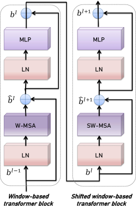
Figure 4: Swin transformer block

III-B2 Keypoints Detection and Description

The 3D dense feature output by Dense Feature Extraction is simultaneously utilized for both keypoint detection and description. To enhance their accuracy and robustness, we introduce soft detection score under global semantic attention in this step. Firstly, utilizing cyclic-shift window to achieve global contextual attention, the quantity of batched windows remains identical to that of regular window partitioning, ensuring efficiency, Swin Transformer[50] demonstrated it. The windows are organized in a way that divides the image evenly without overlapping. Assuming that each window contains $P\times P$ patches, the computational complexity of the global multi-head self-attention (MSA) module and the window-based model on an image consisting of $h\times w$ patches is as follows:

$$\text{MSA: }O(4hwC^{2}+2(hw)^{2}C),$$ (6)

$$\text{W-MSA: }O(4hwC^{2}+2M^{2}hwC),$$

the former exhibits quadratic complexity with respect to the patch count hw, while the latter maintains linearity when the fixed value of $P$ is used (defaulted to 7). Global self-attention computations are typically impractical for a large $hw$, whereas window-based self-attention is scalable.

Similar to the previous works [51, 19], a relative position bias matrix is adopted in each head computing similarity:

$$Attention(Q,K,V)=SoftMax(\frac{QK^{T}}{\sqrt{d}}+\mathcal{A})V,$$ (7)

where $Q,K,V\in{\mathbb{R}}^{W^{2}\times d}$ denote the query, key and value matrices. $W^{2}$ and $d$ represent the number of patches in a window and the dimension of the $query$ or $key$, respectively. And, the values in $\mathcal{A}$ are taken from the bias matrix $\hat{\mathcal{A}}\in{\mathbb{R}}^{(2B-1)\times(2B+1)}$ instead of traditional $\mathcal{A}\in{\mathbb{R}}^{(B^{2}\times B^{2}}$, because of the relative position along each axis lies in the range $[-B+1,B-1]$.

Furthermore, the above feature extraction function $\mathcal{F}$ can be conceptualized as comprising $n$ different feature detection functions $\mathcal{R}_{k}$, each producing a 2D response map $R_{k}$. These detection response maps are analogous to the Difference-of-Gaussians (DoG) responses found in SIFT. We post-process these raw scores through our soft detection score to select only a subset of locations as the output keypoints. This process is detailed below. Contrary to traditional feature detectors that reduce detection map through a straightforward non-local-maximum suppression, in our case, there are multiple detection maps $R_{k}(k=1,...,n)$, and a detection can occur on any of them. Therefore, for a point $p_{(i,j)}$ to be detected, we require:

$${R_{ij}}^{k}\mbox{ is a local max in }R^{k},\mbox{with }k=\mathop{\arg\max}\limits_{t}{R_{ij}}^{t}.$$ (8)

Obviously, for each pixel $(i,j)$, first selecting the most preeminent detector $\mathcal{R}^{k}$ (channel selection), and then verifying whether a local-maximum exists at position $(i,j)$ on that specific detector’s response map ${R}^{k}$.

In order to take both criteria into account, we maximize the product of both scores across all feature maps $k$ to obtain a single score map. Furthermore, we enhance this detection strategy to make it compatible with neural network backpropagation. As illustrated in following formula:

$$\left\{\begin{aligned} \phi_{ij}&=\max\limits_{k}(\eta_{ij}^{k}\zeta_{ij}^{k}),\\ \eta_{ij}^{k}&=\frac{exp(R_{ij}^{k})}{\sum_{(i^{{}^{\prime}},j^{{}^{\prime}})\in\mathcal{M}(i,j)}exp(R_{i^{{}^{\prime}}j^{{}^{\prime}}}^{k})},\\ \zeta_{ij}^{k}&=\frac{R_{ij}^{k}}{\max\limits_{t}R_{ij}^{t}},\end{aligned}\right.$$ (9)

where $\phi_{ij}$ represents a soft-local-max, $\mathcal{M}(i,j)$ is the set of $9$-pixel neighborhood of $(i,j)$, including the pixel itself. And $\zeta_{ij}^{k}$ computes a ratio-to-max for soft channel selection.

Finally, the soft detection score $s_{ij}$ at a pixel $(i,j)$ with global semantic attention is obtained by performing an image-level normalization:

$$s_{(i,j)}=\frac{\phi_{ij}}{\sum\limits_{i{{}^{\prime}},j{{}^{\prime}}}\phi_{i{{}^{\prime}}j{{}^{\prime}}}}.$$ (10)

III-B3 Jointly Optimizing Detection and Description

This section describes the loss for detection and description optimizing. In detection, we aim for keypoint repeatability across changes in viewpoint and illumination, while in description, we seek distinctive descriptors to prevent mismatches. In order to meet these requirements, we propose an extend triplet edge ranking loss with pixel geometric attention. We will begin by revisiting the triplet edge ranking loss and then introduce our extended version that combines both detection and description aspects.

For a pair of query and reference images, $(I_{q}$ and $I_{r}^{1})$, and a correspondence $c\colon X\leftrightarrow Y$ between them, where $X\in I_{q},Y\in I_{r}^{1}$, our extend triplet margin ranking loss aims to minimize the distance between corresponding descriptors ${\hat{R}}_{X}^{(1)}$ and ${\hat{R}}_{Y}^{(2)}$, while maximizing the distance to other confusing descriptors ${\hat{R}}_{N_{1}}^{(1)}$ or ${\hat{R}}_{N_{2}}^{(2)}$ in either image, which might exist due to presence of similar-looking image structures. Towards this objective, we define the positive descriptor distance $d_{p(c)}$ between the corresponding descriptors as:

$$d_{p(c)}={\lVert{\hat{R}}_{A}^{(1)}-{\hat{R}}_{B}^{(2)}\rVert}_{2}.$$ (11)

The negative distance $d_{n(c)}$, which accounts for the most confounding descriptor for either ${\hat{R}}_{X}^{(1)}$ or ${\hat{R}}_{Y}^{(2)}$, is defined as:

$$d_{n(c)}=\min{\Bigl{(}{\lVert{\hat{R}}_{N_{1}}^{(1)}-{\hat{R}}_{N_{2}}^{(2)}\rVert}_{2},{\lVert{\hat{R}}_{X}^{(1)}-{\hat{R}}_{Y}^{(2)}\rVert}_{2}\Bigr{)}},$$ (12)

where the negative samples ${\hat{R}}_{N_{1}}^{(1)}$ and ${\hat{R}}_{N_{2}}^{(2)}$ are the hardest negatives that lie outside of a square local neighbourhood of the correct correspondence:

$$N_{1}=\mathop{\arg\min}\limits_{P\in I_{q}}{\lVert{\hat{R}}_{P}^{(1)}-{\hat{R}}_{B}^{(2)}\rVert}_{2}s.t.\lVert P-X\rVert_{\infty}\textgreater K,$$ (13)

and similarly for $N_{2}$. The triplet margin ranking loss $\mathcal{L_{M}}$ for a margin $\mathcal{M}$ can be defined as:

$$\mathcal{L_{M}}(c)=\max(0,margin+d_{p(c)}^{2}-d_{n(c)}^{2}).$$ (14)

To further encourage detection repeatability against appearance variations, a soft detection term is incorporated into the triplet margin ranking loss as follows:

$$\mathcal{L}(I_{q},I_{r})=\sum\limits_{c\in\mathcal{C}}\frac{s_{c}^{(1)}s_{c}^{(2)}}{\sum_{q\in\mathcal{C}}s_{q}^{(1)}s_{q}^{(2)}}\mathcal{L_{M}}(p(c),n(c)),$$ (15)

where $s_{c}^{(1)}$ and $s_{c}^{(2)}$ are the soft detection scores 10 at points $X$ and $Y$ in $I_{q}$ and $I_{r}^{1}$, respectively, and $\mathcal{C}$ is the set of all correspondences between $I_{q}$ and $I_{r}^{1}$.

The proposed loss calculates a weighted average of $\mathcal{M}$ for all matches, determined by their soft detection scores. Consequently, to minimize the loss, correspondences that exhibit higher distinctiveness (indicated by a lower margin term) will receive elevated relative scores, and conversely, correspondences with higher relative scores are incentivized to possess descriptors that stand out from the rest.

III-C Reranking and Matching

In stereo matching, using RANdom SAmple Consensus (RANSAC) or similar geometric constraint algorithms is an effective method for refining matching points. However, when the set of matching point pairs to be refined contains a large number of significantly mismatched points, the RANSAC algorithm’s random sampling and iterative approach can become highly unstable due to the influence of these erroneous matches. Therefore, prior to applying geometric constraints, it is necessary to perform coarse refinement of the matching point pairs.

This section will introduce the details of our stereo matching and reranking strategy based on the keypoints and descriptors output by the above Swin-Descriptors.

III-C1 Adaptive Distance Filter

Through the Fast Library for Approximate Nearest Neighbors (FLANN) algorithm, we search for the nearest neighboring matching pair, which includes the closest first matching point and the second closest second matching point, from the set of matching pairs to be filtered. Typically, for the $j$-th matching pair in the set to be filtered, a smaller Euclidean distance ($dis_{j}$) between the first matching point and a larger Euclidean distance ($dis_{j}^{{}^{\prime}}$) between the second matching point implies better match quality. Traditional algorithms often employ a fixed ratio factor $t$ as a threshold, i.e., when $dis_{j}<t\textperiodcentered dis_{j}^{{}^{\prime}}$, the pair is selected as a candidate matching pair. However, due to substantial differences in image quality arising from different sensors and temporal factors, it is challenging to anticipate the range of Euclidean distance differences when searching for Euclidean space distances with deep learning features.

As a result, for each pair of images, it is typically necessary to manually adjust the $t$ threshold value repeatedly to achieve suitable values for filtering high-quality matching pairs. To address this issue and improve the algorithm’s adaptability, this paper introduces a dynamic and adaptive Euclidean distance constraint method. This method statistically analyzes the data of the matching pairs to be refined and automatically configures corresponding parameters based on data characteristics.

First, from the $N$ matching pairs retrieved by the FLANN search, which may include a significant number of mismatches, we compute the mean difference between the distances of the first matching point and the second matching point.

$$dis^{*}=(\sum_{j=1}^{N}dis_{j}^{{}^{\prime}}-dis_{j})/N.$$ (16)

For each matching pair to be filtered, the removal condition is based on the difference between the first distance ($dis_{j}$) being smaller than the second distance ($dis_{j}^{{}^{\prime}}$) and the mean difference ($dis^{*}$) in distances. The formula is as follows:

$$dis_{j}\textless dis_{j}^{{}^{\prime}}-dis^{*}.$$ (17)

The algorithm utilizes the mean difference in distances calculated from the data as a discriminative comparison criterion. This approach adapts well to variations between image pairs from different domains, enabling effective initial filtering to retain high-quality matching points. At the same time, enhancing the stability of the RANSAC output.

III-C2 RANSAC via Affine Model

In RANSAC, the selection of geometric constraint relationships should be based on the imaging geometry of the images being matched. In practical engineering applications, it is advisable to use rigorous constraint models whenever possible. For instance, when dealing with images captured from Area-Array Cameras, models like homography matrices or essential matrices are often suitable constraints. On the other hand, for satellite images captured from Line-Array Cameras, constraints like the RPC (Rational Polynomial Coefficients) model or polynomial models based on kernel lines are commonly used.

In our experiments, given the relatively large photographic distance of the selected remote sensing images, minimal ground height differences, and a small image region, we chose to utilize the affine transformation model. This choice allows for accommodating various types of transformations, including scaling, translation, rotation, and shearing, between image pairs originating from different imaging models.

III-C3 Reranking

After obtain the distinctive keypoints and associated stereo matching relationships, we calculate the average pixel distance of final correspondences between the query image and the candidate images. Subsequently, we return the top 5 reference images with the smallest average distance as the refined retrieval candidates.

III-D Pose Estimation

After obtaining stereo matching relationships between query and candidate images, the precise geolocation of UAV can be calculated by solving a PnP problem, as illustrated in Fig. 2(c).

First of all, given the geo-tags and the keypoints of the five satellite images, it is not difficult to obtain the GPS coordinates of these keypoints, that is, the GPS coordinates of corresponding keypoints in the query image. And then, by solving PnP problem of the 2D and 3D correspondences of keypoints in the query image, the camera pose of UAV is estimated.

By leveraging the PnP principle, we can establish the motion model of the camera’s coordinate system relative to the world coordinate system, which corresponds to the camera pose. And this camera pose represents the drone’s pose, the translation component of this pose provides the precise geolocation of this drone.

To find the optimal camera pose, we formulate a nonlinear least squares problem based on the re-projection error. This problem aims to minimize the sum of errors between the $n$ matching points re-projected pixel coordinates in the image plane and their corresponding projected pixel coordinates computed using the camera pose and the corresponding 3D point positions. The re-projection error is defined as follows:

$$\boldsymbol{T^{*}}=\mathop{\arg\min}\limits_{\boldsymbol{T}}\frac{1}{2}\sum_{i=1}^{n}{\left\lVert\boldsymbol{p}^{i}-\frac{1}{s_{i}}\boldsymbol{KT}\boldsymbol{P}_{i}^{W}\right\rVert}_{2}^{2}.$$ (18)

In the equation, $\boldsymbol{K}$ and $\boldsymbol{T}$ respectively represents the camera intrinsic matrix and transformer matrix, $\boldsymbol{p}^{i}$ represents the pixel coordinates of a point, $\boldsymbol{P}_{i}^{W}$ represents the corresponding world coordinates of a matching point, and $s_{i}$ is the depth of $\boldsymbol{p}^{i}$ in camera coordinate system. These two sets of coordinates represent different representations of the same spatial point in different coordinate systems. $\frac{1}{s_{i}}\boldsymbol{KT}\boldsymbol{P}_{i}^{W}$ is the coordinates of the point in the world coordinate system, and is the projected coordinates in the pixel coordinate system, obtained through the camera’s motion pose.

By minimizing the re-projection error, we can obtain an estimate of the optimal camera pose $\boldsymbol{T^{*}}$, that is, the ultimate precise geolocation.

IV Experiments

In this section, we run extensive experiments to show the robustness and accuracy of the proposed CurriculumLoc compared to existing state-of-the-art techniques by evaluating on two challenging datasets. In what follows, we present implementation details, datasets, evaluation metrics, performance comparisons and ablation studies.

IV-A Implementation Details

We implemented our approach in Pytorch and resize all images to $500\times 500$ pixels.

IV-A1 Training Details

During training, the last layer of Swin-Descriptors was fine-tuned for 50 epochs. We employed the Adam optimizer with an initial learning rate of $10^{-3}$, which was subsequently halved every 10 epochs. For each pair, we selected a random $224\times 224$ crop centered around a correspondence point, and the patch size was set to 4. We utilized a batch size of 1 and ensured that the training pairs contained a minimum of 128 correspondences to yield meaningful gradients.

IV-A2 Test Details

At test time, to increase the resolution of the feature maps, we remove the last patch merging layer. This adjustment result in feature maps with one-fourth the resolution of the input, enabling the detection of more potential keypoints and improving localization. The positions of the detected keypoints were refined locally at the feature map level, following a methodology akin to that employed in SIFT. Finally, the descriptors were bilinearly interpolated at the refined positions.

IV-A3 Datasets

We evaluated our approach on one public benchmark dataset: ALTO and our self-collected dataset: TerraTrack. All of these datasets contain various challenging environmental variations. Table I summarizes the qualitative nature of them. All images are resized to 500 × 500 while evaluation.

TABLE I: Summary of datasets used for training and evaluation. + indicates that the dataset contains the particular environmental variation, and - is the opposite.

Dataset		Environment			Variation
		Urban	Suburban	Natural	Viewpoint	Illumination	Scale	Texture	Domain
ALTO [52]			✓	✓	+	+	-	+	+
TerraTrack	mavic-river		✓	✓	+	+	-	-	+
	mavic-hongkong	✓			+	+	-	-	+
	mavic-factory		✓		+	+	-	-	+
	mavic-fengniao		✓		+	+	-	-	+
	inspire1-rail-kfs		✓	✓	+	+	-	+	+
	phantom3-grass-kfs		✓	✓	+	+	-	+	+
	phantom3-centralPark-kfs		✓	✓	+	+	-	-	+
	phantom3-npu-kfs		✓		+	+	+	-	+
	phantom3-freeway-kfs		✓	✓	+	+	-	+	+
	phantom3-village-kfs		✓	✓	+	+	-	-	+
	gopro-npu-kfs		✓		+	+	+	-	+
	gopro-saplings-kfs		✓		+	+	-	+	+
	mavic-xjtu	✓			+	+	-	-	+
	phantom3-huangqi-kfs		✓	✓	+	+	-	+	+
	mavic-npu		✓		+	+	+	-	+
	mavic-road		✓		+	+	-	-	+

For our TerraTrack, a self-made hexacopter and a DJI Phantom3 are used to record the query images in different terrains and heights, and the reference images derive from the satellite imagery of Google Maps. The current dataset is available at the link given in the Abstract, and can serve for cross-domain geolocalization algorithm validation. However, it’s important to note that the dataset, while valuable, is not extensive, and the full dataset is forthcoming.

In order to generate training data for pixel-wise correspondences, we utilized our TerraTrack dataset, which comprises 16 distinct scenes reconstructed from a total of 5,848 UAV images and 23,392 satellite images employing COLMAP [53, 54].

To extract correspondences, we initially evaluated all pairs of images exhibiting a minimum of 50% overlap in the sparse SfM point cloud. For each pair, we projected all depth-informed points from the second image onto the first image. A depth-check procedure, relative to the depth map of the first image, was executed to eliminate occluded pixels. This dataset was subsequently divided into a validation dataset, consisting of 359 image pairs (from two scenes, each containing fewer than 100 image pairs), and a training dataset comprising the remaining 14 scenes.

IV-B Comparison with Other Methods

IV-B1 Compared Methods

We compare our rerank results with several state-of-the-art vision place recognition algorithms, including retrieval with global descriptors: NetVLAD [9] and SFRS [55] and two-stage pipeline (global retrieval and rerank based local descriptors): Patch-NetVLAD [10], DELG [13] and TransVLAD [12]. For Patch-NetVLAD, we evaluated both 2048 and 4096 descriptor dimension, denoted as Patch-NetVLAD-2048 and Patch-NetVLAD-4096 respectively. Moreover, we also compared against a latest global-based method GCG-Net [11] and a two stage pipeline TransVLAD [12]. GCG-Net [11] employed graph structure to represent global descriptors and TransVLAD [12] extracted feature maps by a transformer based network. For all methods, we use recall@N metric which computes the percentage of query UAV images that are correctly localized. A query image is considered to have been correctly positioned if at least one of the first $N$ reference images is within a threshold distance from the query’s ground truth location.

IV-B2 Metrics

For the ALTO and TerraTrack datasets, we employ the recall@N metric, which calculates the percentage of query images that achieve accurate localization. A query image is considered as correctly localized if at least one of the top N ranked reference images is within a threshold distance from the ground truth location of the query. We respectively set the threshold distance at 20 and 50 meters, based on the flight altitude and range specifications in our datasets. The setting of these two distance thresholds provides a more comprehensive evaluation of the algorithm’s robustness.

IV-B3 Results

The quantitative results of ALTO and TerraTrack are shown in Table II and Table III. In addition, Fig. 5 and Fig. 6 show the recall@1 preformance on ALTO and TerraTrack. In conclusion, compare against other retrieval-based methods our two stage pipeline achieves a significant improvement with 62.6%/94.5% of R@1 and 92.6%/99.7% of R@5 in ALTO with metric distance of $20m/50m$, and 62.7%/67.9 % of R@1 in TerraTrack with metric distance of $20m/50m$, respectively. Fig. 7 and Fig. 8 show the the top-1 retrieval reference images of query images by our model with NetVLAD, SFRS, GCG-Net, Patch-NetVLAD-2048, Patch-NetVLAD-4096, DELG and TransVLAD on challenging scenes, besides different domian (query images from UAV capture, reference images is a selection of satellite images), repeated texture, illumination and viewpoint changed, and pereceptual aliasing).

TABLE II: The results of local match with other place recognition methods (dist=$20m$)

Methods		ALTO				TerraTrack
		R@1	R@5	R@10	R@20	R@1	R@5	R@10	R@20
Global	NetVLAD [9]	20.4	58.3	77.1	88.4	22.8	48.8	57.8	67.8
	SFRS [55]	25.4	60.1	78.6	91.4	22.9	49.1	58.1	68.9
	GCG-Net [11]	11.8	36.9	51.9	66.0	24.8	49.2	56.1	62.4
Local	Patch-NetVLAD-2048 [10]	33.9	78.3	91.2	95.6	56.0	68.6	72.3	74.4
	Patch-NetVLAD-4096 [10]	31.1	74.8	90.4	94.9	53.8	64.7	68.1	69.2
	DELG [13]	35.9	79.9	92.3	95.6	58.2	68.3	71.9	73.6
	TransVLAD [12]	34.7	78.8	91.9	95.3	58.4	67.9	72.1	73.8
Ours		$\mathbf{62.6}$	$\mathbf{92.6}$	$\mathbf{95.6}$	$\mathbf{96.1}$	$\mathbf{62.7}$	$\mathbf{69.2}$	70.2	72.7

TABLE III: The results of local match with other place recognition methods (dist=$50m$)

Methods		ALTO				TerraTrack
		R@1	R@5	R@10	R@20	R@1	R@5	R@10	R@20
Global	NetVLAD [9]	62.0	88.3	94.5	98.0	40.1	61.5	71.4	78.9
	SFRS [55]	64.6	90.6	93.4	98.0	44.7	61.6	72.5	75.6
	GCG-Net [11]	57.7	72.2	79.7	84.2	46.1	62.1	65.1	69.2
Local	Patch-NetVLAD-2048 [10]	85.0	97.4	98.8	99.8	67.7	74.4	78.6	82.6
	Patch-NetVLAD-4096 [10]	82.9	96.9	98.2	99.0	67.2	72.0	76.5	79.1
	DELG [13]	87.7	97.9	99.2	99.6	67.6	75.1	78.6	82.4
	TransVLAD [12]	83.6	96.1	98.6	98.6	67.3	73.5	78.9	81.9
Ours		$\mathbf{94.5}$	$\mathbf{99.7}$	$\mathbf{99.8}$	$\mathbf{99.8}$	$\mathbf{67.9}$	74.3	77.9	78.9

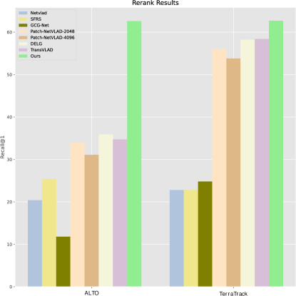
Figure 5: Comparison results of retrieval recall@1 with dist=20$m$.

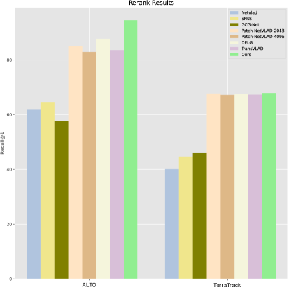
Figure 6: Comparison results of retrieval recall@1 with dist=50$m$.

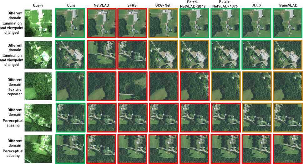
Figure 7: Comparison of retrieval results on ALTO validation dataset. In these challenging examples, Our CurriculumLoc successfully retrieves the matching database image, while all other methods produce false results.

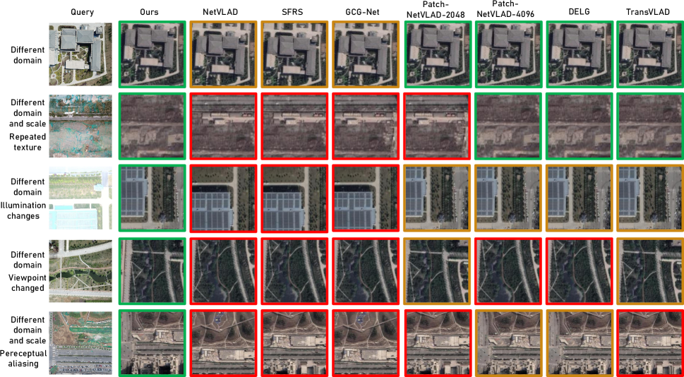
Figure 8: Comparison of retrieval results on TerraTrack validation dataset. In these challenging examples, Our CurriculumLoc successfully retrieves the matching database image, while all other methods produce false results.

The above comparative experiments show that our method achieves state-of-the-art localization results in the rerank stage, and also demonstrates the effectiveness of our feature detection and extraction module Swin-Descriptors.

IV-C Ablation Study

IV-C1 Initial Retrieval Candidates Number

Theoretically, the rerank efficiency is inversely proportional to the number of input candidate images, but the positioning accuracy of the rearrangement results is directly proportional to it. Fig. 9 shows the impact of different number of input candidates on the rerank result (recall@1) on the ALTO dataset. It is evident that $n=50$ is the optimal number of candidate images.

This experiment also shows that the initial retrieval in our pipeline can saving rerank efficiency of matching. Using top $50$ initial candidates to rerank can significantly improve the performance of recall@1 from 20.4%/62.0% to 62.6%/94.5% with distance threshold of $20m/50m$.

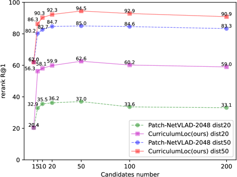
Figure 9: The rerank recall@1 preformance of our CurriculumLoc and Patch-NetVLAD-2048 with different candidate numbers on ALTO.

IV-C2 Modules in Rerank and Match

To verify the effectiveness of our Swin-Descriptors, transform model in dynamic filter and rerank strategy, we conduct several ablation experiments to further validate the design and pipeline of our algorithm. The results on ALTO and TerraTrack datasets are reported in Table IV.

TABLE IV: Ablations with our Swin-Descriptors, dynamic filter strategy and project model on ALTO and TerraTrack datasets.

Methods		dist20				dist50
		R@1	R@5	R@10	R@20	R@1	R@5	R@10	R@20
ALTO	VGG-16 + $F_{num}$ + ADF + affine	43.6	78.9	90.8	94.6	78.9	90.3	95.7	98.0
	VGG-16 + $F_{dist}$ + ADF + affine	50.4	85.6	92.6	94.6	86.4	92.6	96.8	98.0
	SW + $F_{num}$ + ADF + affine	54.4	88.8	94.6	95.2	88.7	95.6	97.8	98.2
	SW + $F_{dist}$ + affine	62.1	92.2	95.4	96.1	92.9	98.7	99.5	99.8
	SW + $F_{dist}$ + ADF + euclidean	57.8	91.2	94.4	93.6	90.9	96.8	98.8	99.2
	SW + $F_{dist}$ + ADF + similarity	61.8	92.6	95.6	96.1	93.6	99.6	99.8	99.8
	SW + $F_{dist}$ + ADF + project	62.3	92.5	95.6	96.1	94.1	99.6	99.8	99.8
	SW + $F_{dist}$ + ADF + affine	62.6	92.6	95.6	96.1	94.5	99.7	99.8	99.8

symmetric Encoder-Decoder Swin Transformer with shifted window attention mechanism and soft detection score strategy Note that SW refers to the proposed symmetric transformer dense feature extraction network with shifted window attention in Swin-Descriptors, while VGG-16 refers to extracting feature by VGG-16 without attention mechanism. $F_{num}$ and $F_{dist}$ refer to re-rank global retrieval results with the number of correspondences or the average pixel distance of all correspondences. ADF refers to our adaptive distance filter brfore RANSAC in dynamic filter. Euclidean, similarity, project, affine are transform model of RANSAC in Geometric Verification. From the results, we can draw the following conclusions. Swin-Descriptors with SW can encode multi-scale level semantic feature and capture local information with global awareness and pixel supervision to improve the rerank performance. In particular, using SW to replace the VGG-16 improves the R@1 performance of our method from 50.4%/78.9% to 62.6%/94.5% on ALTO dataset with metric distance of $20m/50m$, respectively. Rerank the global candidates based on the average pixel distance of all correspondences ($F_{dist}$) is more robust than the number of correspondences($F_{num}$) between query image and candidate image. For example, exploiting the $F_{dist}$ improves the R@1 performance of the $F_{num}$ from 43.6% to 50.4% with VGG-16 and achieves 8.2% improvement at R@1 with SW. Adaptive distance filter (ADF) before RANSAC in Dynamic filter improves the quality of matched keypoints between query and candidate image and thus improves the R@1 from 62.1%(92.9%) to 62.6%(94.5%) with metric distance of $20m/50m$. Among these four transform models in RANSAC, the similarity model, project model, and affine model all exhibit equally strong results in terms of recall@10 and recall@20. However, the affine model outperforms the others, achieving the highest recall@1 and recall@5.

Additionally, as shown in Fig. 10, the contrast of the trained soft detection score map is significantly increased relative to its initial counterpart, which is more helpful in capturing the invariant information in the image.

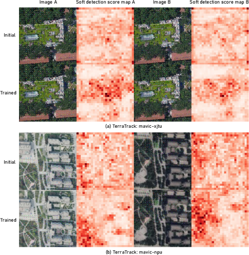
Figure 10: Soft detection scores for different scenes before and after training. White represents low soft-detection scores while red signifies higher ones. The contrast of the trained soft detection score map is significantly increased relative to its initial counterpart, which is more helpful in capturing the invariant information in the image.

IV-C3 Pose Estimation and Localization

The rerank top $5$ candidates and the corresponding matching keypoints pairs enable us to establish matching relationships between candidate images and query image. Solving this cross-domain stereo matching problem enable our CurriculumLoc to return a more accurate position closer to the query, which may not be present in the candidate database.

The visualization of the keypoint correspondences between images pairs from ALTO and TerraTrack dataset is illustrated in Fig. 11. Our Swin-Descriptors detect and describe keypoints are robust to different domain and significant changes in scale, and in textureless regions, the form of our descriptor construction is able to identify correspondences between grass across different domain images.

Figure 11: Final stereo matching results of matched image pairs from ALTO and TerraTrack datatsets in various challenge conditions.

Fig. 12 illustrate the illustrates the improvement in localization accuracy from reranking to pose estimation and location refinement. It also shows the progress from the initial retrieval to the reranking stage.

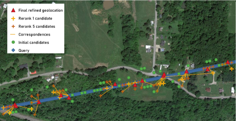
Figure 12: An overhead view of the trajectories generated by our CurriculumLoc is shown on the satellite map at ALTO. The green spot and orange cross are the location of the initial candidates (top-5) from global retrieval and refined candidates (top-5) by rerank. Red markers represent positions after PnP estimation. The orange line segment shows the correspondence between the rerank candidates and query. The blue trace represents the query position of the GPS.

IV-D Localization under Challenging Conditions

The previous experiments showed that our approach through rerank outperforms comparable with the state-of-the-art retrieval methods and further improve the accuracy through pose estimation. In this experiment, we show that our approach is enough robust to be applied under a challenging condition: Localizing images under severe illumination changes and in different scale and domain. Fig. 13 and Fig. 14 show the trajectories of the recall@1 position and the final refined position. In particular, Fig. 14 displays the position of the axis of x, y, and the x-axis and y-axis represent east and north coordinates in UTM system, respectively. It can be seen that our method has well refined the recall@1 position results. The mean, std, median, rmse, and APE results of the final position by our CurriculumLoc are shown in Fig. 15. It can be seen that only using our visual geolocalization solution, the mean error of localization is less than 10$m$, while the relative flight height of this data is higher than 500 meters, and the std, median, rmse and APE results also demonstrate that our CurriculumLoc is competent for geolocation of practical UAV applications.

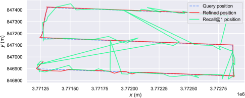
Figure 13: The trajectory of rerank recall@1 and final refined position.

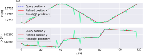
Figure 14: The trajectory of rerank recall@1 and final refined position in different axis.

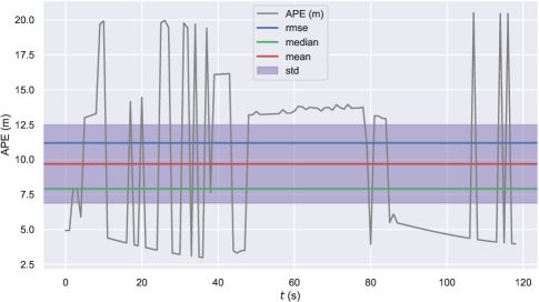
Figure 15: The absolute position error of final refined position.

V Conclusion

Our designed Swin Descriptors address the issue of context information loss caused by the limited receptive field of CNNs in dense feature extraction. It constructs an Encoder-Decoder transformer and enhances interaction between different windows through shift window attention in Swin Transformer. This enables the extraction of more robust and reliable invariant features under extreme weather conditions, viewpoint changes, and scale variations. Furthermore, our soft detection score map is detected from dense feature map and optimized by pixel geometric supervision, our keypoints is distinctive and corresponding descriptors enable fully enjoy global semantic awareness and local geometric verification. We utilizing these ketpoints and descriptors to rerank and estimate a more precise position. Different from existing geo-localization algorithms that can only return the nearest neighboring geo-tag in the database, our algorithm provides an accurate global location. Thorough experiments on retrieval-based localization, keypoint detection and matching, localization under challenging conditions, and ablation study validated that our Swin-Descriptors can embrace both distinctive and invariance power and ourCurriculumLoc can outperforms existing cross-domian geolocalization methods. The future works include exploring more efficient backbone networks, as well as integrating our method into practical SLAM and other reconstruction applications.

References

- [1] Torsten Sattler, Akihiko Torii, Josef Sivic, Marc Pollefeys, Hajime Taira, Masatoshi Okutomi, and Tomas Pajdla. Are large-scale 3d models really necessary for accurate visual localization? In 2017 IEEE Conference on Computer Vision and Pattern Recognition (CVPR), Jul 2017.
- [2] Deepak Rajamohan, Jonghyuk Kim, Matt Garratt, and Mark Pickering. Image based localization under large perspective difference between sfm and slam using split sim (3) optimization. Autonomous Robots, 46(3):437–449, 2022.
- [3] Torsten Sattler, Bastian Leibe, and Leif Kobbelt. Efficient and effective prioritized matching for large-scale image-based localization. IEEE Transactions on Pattern Analysis and Machine Intelligence, page 1744–1756, Sep 2017.
- [4] EW Nota, W Nijland, and T de Haas. Improving uav-sfm time-series accuracy by co-alignment and contributions of ground control or rtk positioning. International Journal of Applied Earth Observation and Geoinformation, 109:102772, 2022.
- [5] Guillaume Bresson, Zayed Alsayed, Li Yu, and Sebastien Glaser. Simultaneous localization and mapping: A survey of current trends in autonomous driving. IEEE Transactions on Intelligent Vehicles, page 194–220, Sep 2017.
- [6] Hamid Taheri and Zhao Chun Xia. Slam; definition and evolution. Engineering Applications of Artificial Intelligence, 97:104032, 2021.
- [7] Weifeng Chen, Guangtao Shang, Aihong Ji, Chengjun Zhou, Xiyang Wang, Chonghui Xu, Zhenxiong Li, and Kai Hu. An overview on visual slam: From tradition to semantic. Remote Sensing, 14(13):3010, 2022.
- [8] Abhishek Gupta and Xavier Fernando. Simultaneous localization and mapping (slam) and data fusion in unmanned aerial vehicles: Recent advances and challenges. Drones, 6(4):85, 2022.
- [9] Relja Arandjelovic, Petr Gronat, Akihiko Torii, Tomas Pajdla, and Josef Sivic. Netvlad: Cnn architecture for weakly supervised place recognition. IEEE Transactions on Pattern Analysis and Machine Intelligence, page 1437–1451, Jun 2018.
- [10] Stephen Hausler, Sourav Garg, Ming Xu, Michael Milford, and Tobias Fischer. Patch-netvlad: Multi-scale fusion of locally-global descriptors for place recognition. In 2021 IEEE/CVF Conference on Computer Vision and Pattern Recognition (CVPR), Jun 2021.
- [11] Yu Zhang, Shuhui Bu, Boni Hu, Pengcheng Han, Lean Weng, and Shaocheng Xue. Gcg-net: Graph classification geolocation network. IEEE Transactions on Geoscience and Remote Sensing, 2023.
- [12] Yifan Xu, Pourya Shamsolmoali, Eric Granger, Claire Nicodeme, Laurent Gardes, and Jie Yang. Transvlad: Multi-scale attention-based global descriptors for visual geo-localization. In Proceedings of the IEEE/CVF Winter Conference on Applications of Computer Vision, pages 2840–2849, 2023.
- [13] Bingyi Cao, André Araujo, and Jack Sim. Unifying Deep Local and Global Features for Image Search, page 726–743. Jan 2020.
- [14] Carl Toft, Will Maddern, Akihiko Torii, Lars Hammarstrand, Erik Stenborg, Daniel Safari, Masatoshi Okutomi, Marc Pollefeys, Josef Sivic, Tomas Pajdla, Fredrik Kahl, and Torsten Sattler. Long-term visual localization revisited. IEEE Transactions on Pattern Analysis and Machine Intelligence, page 2074–2088, Apr 2022.
- [15] Yingxiao Xu, Long Pan, Chun Du, Jun Li, Ning Jing, and Jiangjiang Wu. Vision-based uavs aerial image localization: A survey. In Proceedings of the 2nd ACM SIGSPATIAL International Workshop on AI for Geographic Knowledge Discovery, Nov 2018.
- [16] Xing Xin, Jie Jiang, and Yin Zou. A review of visual-based localization. In Proceedings of the 2019 International Conference on Robotics, Intelligent Control and Artificial Intelligence, Sep 2019.
- [17] Daniel DeTone, Tomasz Malisiewicz, and Andrew Rabinovich. Superpoint: Self-supervised interest point detection and description. In 2018 IEEE/CVF Conference on Computer Vision and Pattern Recognition Workshops (CVPRW), Jun 2018.
- [18] Mihai Dusmanu, Ignacio Rocco, Tomas Pajdla, Marc Pollefeys, Josef Sivic, Akihiko Torii, and Torsten Sattler. D2-net: A trainable cnn for joint detection and description of local features. Le Centre pour la Communication Scientifique Directe - HAL - Diderot,Le Centre pour la Communication Scientifique Directe - HAL - Diderot, May 2019.
- [19] Ze Liu, Han Hu, Yutong Lin, Zhuliang Yao, Zhenda Xie, Yixuan Wei, Jia Ning, Yue Cao, Zheng Zhang, Li Dong, et al. Swin transformer v2: Scaling up capacity and resolution. In Proceedings of the IEEE/CVF conference on computer vision and pattern recognition, pages 12009–12019, 2022.
- [20] Kaiming He, Xinlei Chen, Saining Xie, Yanghao Li, Piotr Dollár, and Ross Girshick. Masked autoencoders are scalable vision learners. In Proceedings of the IEEE/CVF conference on computer vision and pattern recognition, pages 16000–16009, 2022.
- [21] Alexander Kirillov, Eric Mintun, Nikhila Ravi, Hanzi Mao, Chloe Rolland, Laura Gustafson, Tete Xiao, Spencer Whitehead, Alexander C Berg, Wan-Yen Lo, et al. Segment anything. arXiv preprint arXiv:2304.02643, 2023.
- [22] Rongtao Xu, Changwei Wang, Shibiao Xu, Weiliang Meng, Yuyang Zhang, Bin Fan, and Xiaopeng Zhang. Domainfeat: Learning local features with domain adaptation. IEEE Transactions on Circuits and Systems for Video Technology, pages 1–1, 2023.
- [23] Sourav Garg, Tobias Fischer, and Michael Milford. Where is your place, visual place recognition? Cornell University - arXiv, 2021.
- [24] Raul Mur-Artal and Juan D. Tardos. Orb-slam2: an open-source slam system for monocular, stereo and rgb-d cameras. IEEE Transactions on Robotics, page 1255–1262, Oct 2017.
- [25] Yong Zhao, Shibiao Xu, Shuhui Bu, Hongkai Jiang, and Pengcheng Han. Gslam: A general slam framework and benchmark. Cornell University - arXiv,Cornell University - arXiv, Feb 2019.
- [26] D.G. Lowe. Object recognition from local scale-invariant features. In Proceedings of the Seventh IEEE International Conference on Computer Vision, Jan 1999.
- [27] Herbert Bay, Andreas Ess, Tinne Tuytelaars, and Luc Van Gool. Speeded-up robust features (surf). Computer vision and image understanding, 110(3):346–359, 2008.
- [28] Ethan Rublee, Vincent Rabaud, Kurt Konolige, and Gary Bradski. Orb: An efficient alternative to sift or surf. In 2011 International Conference on Computer Vision, Nov 2011.
- [29] Yuki Ono, Eduard Trulls, Pascal Fua, and KwangMoo Yi. Lf-net: Learning local features from images. Neural Information Processing Systems,Neural Information Processing Systems, Jan 2018.
- [30] Linguang Zhang and Szymon Rusinkiewicz. Learning to detect features in texture images. In 2018 IEEE/CVF Conference on Computer Vision and Pattern Recognition, Jun 2018.
- [31] Kwang Moo Yi, Eduard Trulls, Vincent Lepetit, and Pascal Fua. LIFT: Learned Invariant Feature Transform, page 467–483. Jan 2016.
- [32] Jerome Revaud, CésarRobertode Souza, Martin Humenberger, and Philippe Weinzaepfel. R2d2: Reliable and repeatable detector and descriptor. Neural Information Processing Systems,Neural Information Processing Systems, Sep 2019.
- [33] Jerome Revaud, Jon Almazan, Rafael Rezende, and Cesar De Souza. Learning with average precision: Training image retrieval with a listwise loss. In 2019 IEEE/CVF International Conference on Computer Vision (ICCV), Oct 2019.
- [34] Janine Thoma, DandaPani Paudel, and LucVan Gool. Soft contrastive learning for visual localization. Neural Information Processing Systems,Neural Information Processing Systems, Jan 2020.
- [35] Filip Radenovic, Giorgos Tolias, and Ondrej Chum. Fine-tuning cnn image retrieval with no human annotation. IEEE Transactions on Pattern Analysis and Machine Intelligence, page 1655–1668, Jul 2019.
- [36] Hyo Jin Kim, Enrique Dunn, and Jan-Michael Frahm. Learned contextual feature reweighting for image geo-localization. In 2017 IEEE Conference on Computer Vision and Pattern Recognition (CVPR), Jul 2017.
- [37] Frederik Warburg, Soren Hauberg, Manuel Lopez-Antequera, Pau Gargallo, Yubin Kuang, and Javier Civera. Mapillary street-level sequences: A dataset for lifelong place recognition. In 2020 IEEE/CVF Conference on Computer Vision and Pattern Recognition (CVPR), Jun 2020.
- [38] Sourav Garg, Niko Sünderhauf, Feras Dayoub, Douglas Morrison, Akansel Cosgun, Gustavo Carneiro, Qi Wu, Tat-Jun Chin, Ian Reid, Stephen Gould, Peter Corke, and Michael Milford. Semantics for robotic mapping, perception and interaction: A survey. Foundations and Trends® in Robotics, page 1–224, Jan 2020.
- [39] Amadeus Oertel, Titus Cieslewski, and Davide Scaramuzza. Augmenting visual place recognition with structural cues. IEEE Robotics and Automation Letters, page 5534–5541, Oct 2020.
- [40] Tobias Fischer and Michael Milford. Event-based visual place recognition with ensembles of temporal windows. IEEE Robotics and Automation Letters, page 6924–6931, Oct 2020.
- [41] Sourav Garg, Ben Harwood, Gaurangi Anand, and Michael Milford. Delta descriptors: Change-based place representation for robust visual localization. IEEE Robotics and Automation Letters, page 5120–5127, Oct 2020.
- [42] Yu Zhang, Shuhui Bu, Boni Hu, Pengcheng Han, Lean Weng, and Shaocheng Xue. Gcg-net: Graph classification geolocation network. IEEE Transactions on Geoscience and Remote Sensing, 61:1–13, 2023.
- [43] Gabriele Berton, Carlo Masone, and Barbara Caputo. Rethinking visual geo-localization for large-scale applications.
- [44] Giorgos Tolias, Tomas Jenicek, and Ondřej Chum. Learning and aggregating deep local descriptors for instance-level recognition, page 460–477. Jan 2020.
- [45] Hyeonwoo Noh, Andre Araujo, Jack Sim, Tobias Weyand, and Bohyung Han. Large-scale image retrieval with attentive deep local features. In 2017 IEEE International Conference on Computer Vision (ICCV), Oct 2017.
- [46] Karen Simonyan and Andrew Zisserman. Very deep convolutional networks for large-scale image recognition. International Conference on Learning Representations,International Conference on Learning Representations, Jan 2015.
- [47] Jia Deng, Wei Dong, Richard Socher, Li-Jia Li, Kai Li, and Li Fei-Fei. Imagenet: A large-scale hierarchical image database. In 2009 IEEE Conference on Computer Vision and Pattern Recognition, Jun 2009.
- [48] Nahian Siddique, Sidike Paheding, Colin P Elkin, and Vijay Devabhaktuni. U-net and its variants for medical image segmentation: A review of theory and applications. Ieee Access, 9:82031–82057, 2021.
- [49] Ibraheem Alhashim and Peter Wonka. High quality monocular depth estimation via transfer learning. arXiv preprint arXiv:1812.11941, 2018.
- [50] Ze Liu, Yutong Lin, Yue Cao, Han Hu, Yixuan Wei, Zheng Zhang, Stephen Lin, and Baining Guo. Swin transformer: Hierarchical vision transformer using shifted windows. In 2021 IEEE/CVF International Conference on Computer Vision (ICCV), Oct 2021.
- [51] Li Yuan, Yunpeng Chen, Tao Wang, Weihao Yu, Yujun Shi, Zi-Hang Jiang, Francis EH Tay, Jiashi Feng, and Shuicheng Yan. Tokens-to-token vit: Training vision transformers from scratch on imagenet. In Proceedings of the IEEE/CVF international conference on computer vision, pages 558–567, 2021.
- [52] Ivan Cisneros, Peng Yin, Ji Zhang, Howie Choset, and Sebastian Scherer. Alto: A large-scale dataset for uav visual place recognition and localization. Jul 2022.
- [53] Johannes L Schönberger, Enliang Zheng, Jan-Michael Frahm, and Marc Pollefeys. Pixelwise view selection for unstructured multi-view stereo. In Computer Vision–ECCV 2016: 14th European Conference, Amsterdam, The Netherlands, October 11-14, 2016, Proceedings, Part III 14, pages 501–518. Springer, 2016.
- [54] Johannes L Schonberger and Jan-Michael Frahm. Structure-from-motion revisited. In Proceedings of the IEEE conference on computer vision and pattern recognition, pages 4104–4113, 2016.
- [55] Yixiao Ge, Haibo Wang, Feng Zhu, Rui Zhao, and Hongsheng Li. Self-supervising Fine-Grained Region Similarities for Large-Scale Image Localization, page 369–386. Jan 2020.