Shakhov-type extension of the relaxation time approximation
in relativistic kinetic theory and second-order fluid dynamics

Abstract

We present a relativistic Shakhov-type generalization of the Anderson-Witting relaxation time model for the Boltzmann collision integral to modify the ratio of momentum diffusivity to thermal diffusivity. This is achieved by modifying the path on which the single particle distribution function $f_{{\mathbf{k}}}$ approaches local equilibrium $f_{0{\mathbf{k}}}$ by constructing an intermediate Shakhov-type distribution $f_{{\rm S}{\mathbf{k}}}$ similar to the 14-moment approximation of Israel and Stewart. We illustrate the effectiveness of this model in case of the Bjorken expansion of an ideal gas of massive particles and the damping of longitudinal waves through an ultrarelativistic ideal gas.

1 Introduction

The relativistic Boltzmann equation, $k^{\mu}\partial_{\mu}f_{\mathbf{k}}=C[f]$, determines the space-time evolution of a local invariant distribution function $f_{\mathbf{k}}=f(k^{\mu},x^{\mu})$, where $C[f]$ is the collision term specifying the interaction among constituents. The relaxation time approximation (RTA) introduced by Anderson and Witting (AW) [1, 2] as a proper relativistic generalization of the Bhatnagar-Gross-Krook (BGK) model [3], approximates the main features of $C[f]$ for both analytic and numeric computations [4, 5, 6, 7, 8, 9, 10, 11, 12, 13, 14, 15, 16]. Such relaxation-time models share the common caveat that the first-order transport coefficients are related to a single energy-independent relaxation time, $\tau_{R}$. In the BGK model, the Prandtl number $\mathrm{Pr}$, representing a ratio of viscosity to thermal diffusivity, is fixed at $1$, while most ideal gases have $\mathrm{Pr}=2/3$. This limitation was remedied in the extension proposed by Shakhov [17, 18] by introducing another new parameter that allows $\mathrm{Pr}$ to be controlled independently of $\tau_{R}$. This simple modification already leads to a remarkably good agreement with the solutions of the Boltzmann equation and with experimental data, while the BGK model has significant deviations from both [19, 20, 21, 22].

In this paper, we introduce the relativistic Shakhov model as an extension of the AW model, offering additional energy-independent relaxation times that are related to the corresponding first-order transport coefficients, the bulk viscosity $\zeta$, particle diffusion $\kappa$ and shear viscosity $\eta$. This modified collision term, significantly extends the applicability of kinetic RTA models and allows to study different parameterizations of the first-order transport coefficients in various physical phenomena such as the baryon diffusion [23], and the study of bulk and shear viscosities [24, 25] in high-energy heavy-ion collisions.

The improvements compared to the AW model will be shown by comparing the numerical solutions of the kinetic model with solutions of Israel-Stewart-type second-order fluid dynamics in two different benchmarks: the (0+1)–dimensional longitudinally boost-invariant flow of massive particles highlighting the $\zeta/\eta$ ratio, and the damping of sound waves for an ultrarelativistic fluid concerning the $\kappa/\eta$ ratio.

We note that an energy-dependent relaxation time related to the microscopic details of the collisional processes [26, 27, 28] will also modify the first-order transport coefficients [29, 30, 31, 32]. For example, setting $\tau_{R}(x^{\mu},E_{\mathbf{k}})=\tau_{R}(x^{\mu})E_{\mathbf{k}}^{\ell}$ in the AW model provides an extra parameter $\ell$ that can be used to tune either $\zeta/\eta$ or $\kappa/\eta$, while it is not excluded that more elaborate models could tune both of these ratios simultaneously. The Shakhov model introduced in this paper provides an alternative to such AW models with energy-dependent relaxation times.

The detailed derivation of second-order fluid dynamics and the entropy production from the Shakhov model as well as the numerical methods are relegated to the supplementary material.

2 The Anderson-Witting model and transport coefficients

The Boltzmann equation in the Anderson-Witting relaxation-time approximation [1, 2] for the binary collision integral reads

$$k^{\mu}\partial_{\mu}f_{\mathbf{k}}=C_{\rm AW}[f],\quad C_{\rm AW}[f]\equiv-\frac{E_{\mathbf{k}}}{\tau_{R}}\delta f_{\mathbf{k}},$$ (1)

where $E_{\mathbf{k}}=k^{\mu}u_{\mu}$ is the comoving energy of a particle with four-momentum $k^{\mu}$ and rest mass $m_{0}^{2}=k^{\mu}k_{\mu}$, while $\tau_{R}\equiv\tau_{R}(x^{\mu})$ is the local momentum-independent relaxation time. The fluid four-velocity $u^{\mu}=\gamma(1,\mathbf{v})$ is normalized to $u^{\mu}u_{\mu}=1$, where $\gamma=(1-\mathbf{v}^{2})^{-1/2}$. Here, $\delta f_{\mathbf{k}}\equiv f_{\mathbf{k}}-f_{0{\mathbf{k}}}$ denotes the deviation of $f_{\mathbf{k}}$ from its local equilibrium form, the Jüttner distribution [33],

$$f_{0\mathbf{k}}=\left[\exp\left(\beta k^{\mu}u_{\mu}-\alpha\right)+a\right]^{-1}.$$ (2)

where $\alpha=\mu\beta$ and $\beta=1/T$ is the inverse temperature, $\mu$ is the chemical potential, while $a=\pm 1$ for fermions/bosons and $a=0$ for classical Boltzmann particles.

The fluid four-velocity defining the local rest frame is chosen as $u^{\mu}=T^{\mu\nu}u_{\nu}/(u_{\alpha}T^{\alpha\beta}u_{\beta})$, where $T^{\mu\nu}=\int dKk^{\mu}k^{\nu}f_{\mathbf{k}}$ is the energy-momentum tensor, with $dK=[g/(2\pi)^{3}]d^{3}k/k^{0}$ denoting the Lorentz-invariant integration measure in momentum space and $g$ is the degeneracy factor. With respect to $u^{\mu}$, $T^{\mu\nu}$ and the particle four-flow $N^{\mu}=\int dKk^{\mu}f_{\mathbf{k}}$, are decomposed as

$$N^{\mu}=N_{0}^{\mu}+V^{\mu},\quad T^{\mu\nu}=T^{\mu\nu}_{0}-\Pi\Delta^{\mu\nu}+\pi^{\mu\nu},$$ (3)

where $\Delta^{\mu\nu}=g^{\mu\nu}-u^{\mu}u^{\nu}$ is the projector orthogonal to $u^{\mu}$ and $g^{\mu\nu}=\text{diag}(+,-,-,-)$ is the metric tensor. The bulk viscous pressure $\Pi$, the particle diffusion current $V^{\mu}$, and the shear-stress tensor $\pi^{\mu\nu}$ represent dissipative corrections due to $\delta f_{\mathbf{k}}$. $N_{0}^{\mu}$ and $T^{\mu\nu}_{0}$ correspond to the local equilibrium state defined as

$$N^{\mu}_{0}\equiv\int dKk^{\mu}f_{0{\mathbf{k}}}=nu^{\mu},\quad T^{\mu\nu}_{0}\equiv\int dKk^{\mu}k^{\nu}f_{0{\mathbf{k}}}=eu^{\mu}u^{\nu}-P\Delta^{\mu\nu}.$$ (4)

Here, $n\equiv N^{\mu}u_{\mu}=N^{\mu}_{0}u_{\mu}$ is the particle density, $e\equiv T^{\mu\nu}u_{\mu}u_{\nu}=T^{\mu\nu}_{0}u_{\mu}u_{\nu}$ is the energy density, while $P\equiv-T^{\mu\nu}_{0}\Delta_{\mu\nu}/3=P(e,n)$ is the thermodynamic pressure defined by an equation of state.

To evaluate the first-order transport coefficients $\zeta$, $\kappa$ and $\eta$, we apply the Chapman-Enskog method [34], hence from Eq. (1), $\delta f_{\mathbf{k}}$ is considered to be of first order with respect to $\tau_{R}$,

$$\delta f_{\mathbf{k}}\simeq-\frac{\tau_{R}}{E_{\mathbf{k}}}k^{\mu}\partial_{\mu}f_{0{\mathbf{k}}}.$$ (5)

The irreducible moments of $\delta f_{\mathbf{k}}$ are defined as [35]:

$$\rho_{r}^{\mu_{1}\cdots\mu_{\ell}}\equiv\int dKE_{\mathbf{k}}^{r}k^{\langle\mu_{1}}\cdots k^{\mu_{\ell}\rangle}\delta f_{\mathbf{k}},$$ (6)

where $r$ denotes the power of energy $E_{\mathbf{k}}$ and $k^{\left\langle\mu_{1}\right.}\cdots k^{\left.\mu_{\ell}\right\rangle}=\Delta_{\nu_{1}\cdots\nu_{\ell}}^{\mu_{1}\cdots\mu_{\ell}}k^{\nu_{1}}\cdots k^{\nu_{\ell}}$ are the irreducible tensors forming an orthogonal basis [35, 36]. The symmetric and traceless projection tensors of rank $2\ell$, $\Delta_{\nu_{1}\cdots\nu_{\ell}}^{\mu_{1}\cdots\mu_{\ell}}$, are orthogonal to $u^{\mu}$ since they are constructed using the $\Delta^{\mu\nu}$ projector operators.

Through the irreducible moments, $\Pi\equiv-m_{0}^{2}\rho_{0}/3$, $V^{\mu}\equiv\rho_{0}^{\mu}$, and $\pi^{\mu\nu}\equiv\rho_{0}^{\mu\nu}$, we obtain the corresponding first-order approximations for the dissipative quantities,

$$\Pi=-\zeta_{\rm R}\theta,\quad V^{\mu}=\kappa_{\rm R}\nabla^{\mu}\alpha,\quad\pi^{\mu\nu}=2\eta_{\rm R}\sigma^{\mu\nu},$$ (7)

where $\nabla^{\mu}=\Delta^{\mu}_{\nu}\partial^{\nu}$ is the gradient operator, $\theta=\nabla^{\mu}u_{\mu}$ is the expansion rate, and $\sigma^{\mu\nu}=\nabla^{\langle\mu}u^{\nu\rangle}$ is the shear stress tensor. The transport coefficients are proportional to $\tau_{R}$ as:

$$\zeta_{\rm R}=\frac{m_{0}^{2}}{3}\tau_{R}\alpha^{(0)}_{0},\quad\kappa_{\rm R}=\tau_{R}\alpha^{(1)}_{0},\quad\eta_{\rm R}=\tau_{R}\alpha^{(2)}_{0},$$ (8)

where for an ideal gas with conserved particle number the $\alpha^{(\ell)}$ coefficients are

$$\alpha^{(0)}_{r}=-\beta J_{r+1,1}+\frac{1}{G_{22}}[(e+P)G_{2r}-nG_{3r}],$$

$$\alpha^{(1)}_{r}=J_{r+1,1}-\frac{n}{(e+P)}J_{r+2,1},\quad\alpha^{(2)}_{r}=\beta J_{r+3,2}.$$ (9)

When the particle number is not conserved, i.e., $\mu\equiv 0$, then [37]

$$\alpha^{(0)}_{r}=-\beta J_{r+1,1}+\frac{J_{31}}{J_{30}}\beta J_{r+1,0}.$$ (10)

Furthermore $G_{nm}=J_{n0}J_{m0}-J_{n-1,0}J_{m+1,0}$ and the thermodynamic integrals with $\tilde{f}_{0{\mathbf{k}}}=1-af_{0\mathbf{k}}$ are defined as:

$$J_{nq}=\frac{(-1)^{q}}{(2q+1)!!}\int dK\,E_{\mathbf{k}}^{n-2q}\left(\Delta^{\alpha\beta}k_{\alpha}k_{\beta}\right)^{q}f_{0{\mathbf{k}}}\tilde{f}_{0{\mathbf{k}}}.$$ (11)

3 The relativistic Shakhov-type model

The main idea behind the Shakhov-type model [17, 18] is to replace the collision term (1) with

$$C_{\rm S}[f]\equiv-\frac{E_{\mathbf{k}}}{\tau_{R}}(f_{\mathbf{k}}-f_{{\rm S}{\mathbf{k}}})=-\frac{E_{\mathbf{k}}}{\tau_{R}}(\delta f_{\mathbf{k}}-\delta f_{{\rm S}{\mathbf{k}}}),$$ (12)

where $f_{{\rm S}{\mathbf{k}}}=f_{0{\mathbf{k}}}+\delta f_{{\rm S}{\mathbf{k}}}$ replaces $f_{0{\mathbf{k}}}$ in the AW model. This collision term drives $f_{\mathbf{k}}$ towards $f_{{\rm S}{\mathbf{k}}}$, on a time-scale given by $\tau_{R}$, and ultimately towards $f_{0{\mathbf{k}}}$ on a modified path compared to $C_{\rm AW}[f]$ from Eq. (1). We will construct $f_{{\rm S}{\mathbf{k}}}$ such that $\delta f_{{\rm S}{\mathbf{k}}}$ vanishes equivalently in local equilibrium when $\delta f_{\mathbf{k}}=0$.

Applying the Chapman-Enskog method while considering both $\delta f_{{\rm S}{\mathbf{k}}}$ and $\delta f_{\mathbf{k}}$ of first-order with respect to $\tau_{R}$, Eq. (5) is modified to

$$\delta f_{\mathbf{k}}-\delta f_{{\rm S}{\mathbf{k}}}\simeq-\frac{\tau_{R}}{E_{\mathbf{k}}}k^{\mu}\partial_{\mu}f_{0{\mathbf{k}}}.$$ (13)

Alike to Eq. (6), we define the irreducible moments of $\delta f_{{\rm S}{\mathbf{k}}}$,

$$\rho^{\mu_{1}\cdots\mu_{\ell}}_{{\rm S},r}\equiv\int dKE_{\mathbf{k}}^{r}k^{\langle\mu_{1}}\cdots k^{\mu_{\ell}\rangle}\delta f_{{\rm S}{\mathbf{k}}},$$ (14)

hence the first-order relations corresponding to Eq. (13) now read

$$\Pi-\Pi_{\rm S}=-\zeta_{\rm R}\theta,\quad V^{\mu}-V_{\rm S}^{\mu}=\kappa_{\rm R}\nabla^{\mu}\alpha,$$

$$\pi^{\mu\nu}-\pi_{\rm S}^{\mu\nu}=2\eta_{\rm R}\sigma^{\mu\nu}.$$ (15)

Note that, $\Pi_{\rm S}\equiv-m^{2}_{0}\rho_{S,0}/3$, $V^{\mu}_{\rm S}\equiv\rho_{S,0}^{\mu}$, and $\pi^{\mu\nu}_{\rm S}\equiv\rho_{S,0}^{\mu\nu}$ are so far unspecified. We aim to use these new irreducible moments to modify the transport coefficients to the following form,

$$\zeta=\zeta_{\rm R}\frac{\tau_{\Pi}}{\tau_{R}},\quad\kappa=\kappa_{\rm R}\frac{\tau_{V}}{\tau_{R}},\quad\eta=\eta_{\rm R}\frac{\tau_{\pi}}{\tau_{R}},$$ (16)

where $\tau_{\Pi}$, $\tau_{V}$ and $\tau_{\pi}$ are the new $\tau_{R}$-independent relaxation times of bulk viscosity, particle diffusion and shear viscosity, representing parameters of the Shakhov model. In other words, we seek to replace Eqs. (7) by

$$\Pi=-\zeta\theta,\quad V^{\mu}=\kappa\nabla^{\mu}\alpha,\quad\pi^{\mu\nu}=2\eta\sigma^{\mu\nu},$$ (17)

and hence we solve Eqs. (15) and (17) by setting [17, 18]

$$\Pi_{\rm S}=\Pi\left(1-\frac{\tau_{R}}{\tau_{\Pi}}\right),\quad V_{\rm S}^{\mu}=V^{\mu}\left(1-\frac{\tau_{R}}{\tau_{V}}\right),\quad\pi_{\rm S}^{\mu\nu}=\pi^{\mu\nu}\left(1-\frac{\tau_{R}}{\tau_{\pi}}\right).$$ (18)

The conservation equations $\partial_{\mu}N^{\mu}=0$ and $\partial_{\mu}T^{\mu\nu}=0$ are fulfilled when

$$u_{\mu}N^{\mu}=u_{\mu}N^{\mu}_{\rm S},\quad u_{\mu}T^{\mu\nu}=u_{\mu}T^{\mu\nu}_{\rm S},$$ (19)

where $N_{\rm S}^{\mu}=\int dKk^{\mu}f_{{\rm S}{\mathbf{k}}}$ and $T^{\mu\nu}_{\rm S}=\int dKk^{\mu}k^{\nu}f_{{\rm S}{\mathbf{k}}}$. Setting $n=n_{\rm S}$ and $e=e_{\rm S}$ serves to define the local chemical potential and temperature. The local rest frame and $u^{\mu}$ is chosen according to Landau’s definition and leads to $\Delta^{\mu}_{\nu}u_{\lambda}T^{\nu\lambda}_{\rm S}=0$. Note however that in the Shakhov model other definitions for $u^{\mu}$ are possible, as pointed out using a similar construction in Ref. [38].

The conditions from Eqs. (18) and (19) can be written in terms of the irreducible moments

$$\rho_{{\rm S},0} \equiv-\frac{3}{m_{0}^{2}}\Pi_{\rm S}, \rho_{{\rm S},1} \equiv n_{\rm S}-n=0, \rho_{{\rm S},2} \equiv e_{\rm S}-e=0,$$

$$\rho_{{\rm S},0}^{\mu} \equiv V^{\mu}_{\rm S}, \rho_{{\rm S},1}^{\mu} \equiv 0, \rho_{{\rm S},0}^{\mu\nu} \equiv\pi^{\mu\nu}_{\rm S},$$ (20)

while all other irreducible moments of $\delta f_{{\rm S}{\mathbf{k}}}$ are unconstrained.

In order to satisfy Eqs. (20), we construct the relativistic Shakhov distribution $f_{{\rm S}{\mathbf{k}}}$ similarly to the near-equilibrium expansion of Grad [39] and Israel-Stewart [40]. Starting from

$$f_{{\rm S}{\mathbf{k}}}\equiv f_{0{\mathbf{k}}}+\delta f_{{\rm S}{\mathbf{k}}}=f_{0{\mathbf{k}}}+f_{0{\mathbf{k}}}\tilde{f}_{0{\mathbf{k}}}\mathbb{S}_{\mathbf{k}},$$ (21)

we define the Shakhov term $\mathbb{S}_{{\mathbf{k}}}$ as:

$$\mathbb{S}_{\mathbf{k}} \equiv-\frac{3}{m_{0}^{2}}\Pi_{\rm S}\mathcal{H}^{(0)}_{{\mathbf{k}}0}+k_{\langle\mu\rangle}V^{\mu}_{\rm S}\mathcal{H}^{(1)}_{{\mathbf{k}}0}+k_{\langle\mu}k_{\nu\rangle}\pi^{\mu\nu}_{\rm S}\mathcal{H}^{(2)}_{{\mathbf{k}}0}$$

$$=-\frac{3}{m_{0}^{2}}\Pi\left(1-\frac{\tau_{R}}{\tau_{\Pi}}\right)\mathcal{H}^{(0)}_{{\mathbf{k}}0}+k_{\langle\mu\rangle}V^{\mu}\left(1-\frac{\tau_{R}}{\tau_{V}}\right)\mathcal{H}^{(1)}_{{\mathbf{k}}0}$$

$$+k_{\langle\mu}k_{\nu\rangle}\pi^{\mu\nu}\left(1-\frac{\tau_{R}}{\tau_{\pi}}\right)\mathcal{H}^{(2)}_{{\mathbf{k}}0},$$ (22)

The polynomials $\mathcal{H}^{(\ell)}_{{\mathbf{k}}0}$ in energy $E_{\mathbf{k}}$ are constructed to fulfill Eqs. (20) and were introduced in Ref. [35]. In the $14$–moment approximation, these lead to:

$$\mathcal{H}_{{\mathbf{k}}0}^{(0)}= \frac{G_{33}-G_{23}E_{\mathbf{k}}+G_{22}E_{\mathbf{k}}^{2}}{J_{00}G_{33}-J_{10}G_{23}+J_{20}G_{22}},$$

$$\mathcal{H}_{{\mathbf{k}}0}^{(1)}= \frac{J_{31}E_{\mathbf{k}}-J_{41}}{J_{21}J_{41}-J_{31}^{2}},\quad\mathcal{H}_{{\mathbf{k}}0}^{(2)}=\frac{1}{2J_{42}}.$$ (23)

4 Second-order fluid dynamics

The Chapman-Enskog method defines the dissipative fields relating the thermodynamic forces through first-order transport coefficients, resulting in the Navier-Stokes relations, Eqs. (7) and (17). The method of moments by Grad [39], and Israel and Stewart [40], based on an expansion around equilibrium, alike the Shakhov distribution, leads to relaxation-type equations of motion for the dissipative fields $\Pi$, $V^{\mu}$ and $\pi^{\mu\nu}$.

Using the well known $14$–moment approximation of dissipative fluid dynamics [35, 40, 41, 42], the second-order relaxation equations provide closure for the conservation laws. Such relaxation equations can be derived for the Shakhov model, where the additional microscopic time scales introduced through $\delta f_{S{\mathbf{k}}}$ correspond to the relaxation times $\tau_{\Pi}$, $\tau_{V}$, and $\tau_{\pi}$, from a linearized collision integral, e.g. in the case of binary hard-sphere interactions [35, 43]. Consequently, some second-order transport coefficients acquire different values than in the case of the AW model as shown in the Supplementary Material [44].

The equations of motion for the irreducible moments $\rho^{\mu_{1}\cdots\mu_{\ell}}_{r}$ are derived from the Boltzmann equation for an arbitrary collision term. Here, we summarize them up to rank 2, see Eqs. (35)–(37) of Ref. [35]:

$$\dot{\rho}_{r}-C_{{\rm S},r-1} =\alpha^{(0)}_{r}\theta+\text{higher-order terms},$$ (24a)

$$\dot{\rho}^{\langle\mu\rangle}_{r}-C^{\mu}_{{\rm S},r-1} =\alpha^{(1)}_{r}\nabla^{\mu}\alpha+\text{higher-order terms},$$ (24b)

$$\dot{\rho}^{\langle\mu\nu\rangle}_{r}-C^{\mu\nu}_{{\rm S},r-1} =2\alpha^{(2)}_{r}\sigma^{\mu\nu}+\text{higher-order terms}.$$ (24c)

The irreducible moments of the Shakhov collision term $C_{\rm S}[f]$ from Eq. (12) are

$$C^{\mu_{1}\cdots\mu_{\ell}}_{{\rm S},r-1}\equiv\int dKC_{\rm S}[f]E_{\mathbf{k}}^{r-1}k^{\langle\mu_{1}}\cdots k^{\mu_{\ell}\rangle}=-\frac{1}{\tau_{R}}\rho^{\mu_{1}\cdots\mu_{\ell}}_{r}+\frac{1}{\tau_{R}}\rho^{\mu_{1}\cdots\mu_{\ell}}_{{\rm S},r},$$ (25)

where the first term on the right hand side corresponds to the AW collision term, while the second term involves the irreducible moments of $\delta f_{{\rm S}{\mathbf{k}}}$.

The collision matrix $\mathcal{A}^{(\ell)}_{rn}$ is defined by [35, 43]

$$C^{\mu_{1}\cdots\mu_{\ell}}_{{\rm S},r-1}=-\sum_{n}\mathcal{A}^{(\ell)}_{rn}\rho^{\mu_{1}\cdots\mu_{\ell}}_{n},$$ (26)

where the summation over $n$ is unrestricted from below or from above. Using Eq. (25), the collision matrix evaluates to

$$\mathcal{A}^{(\ell)}_{rn}=\frac{\delta_{rn}}{\tau_{R}}-\frac{\delta_{n0}}{\tau_{R}}\left(1-\frac{\tau_{R}}{\tau_{\rm S}^{(\ell)}}\right)\mathcal{F}^{(\ell)}_{-r,0},$$ (27)

where according to Eq. (66) of Ref. [35]

$$\mathcal{F}^{(\ell)}_{rn}=\frac{\ell!}{(2\ell+1)!!}\int dK\,f_{0{\mathbf{k}}}\tilde{f}_{0{\mathbf{k}}}E_{\mathbf{k}}^{-r}(\Delta^{\alpha\beta}k_{\alpha}k_{\beta})^{\ell}\mathcal{H}^{(\ell)}_{{\mathbf{k}}n},$$ (28)

is such that $\mathcal{F}^{(\ell)}_{-r,n}=\delta_{rn}$ for all $0\leq r,n\leq N_{\ell}$, with $\mathcal{H}^{(\ell)}_{{\mathbf{k}}n}$ given in Eqs. (23). Here the different relaxation times are denoted by $\tau_{\rm S}^{(\ell)}$, such that for $\ell=0,1,2$ we define $\tau_{\rm S}^{(0)}=\tau_{\Pi}$, $\tau^{(1)}_{\rm S}=\tau_{V}$ and $\tau^{(2)}_{\rm S}=\tau_{\pi}$. The inverse of the collision matrix is the relaxation-time matrix, satisfying $\sum_{m}\tau^{(\ell)}_{rm}\mathcal{A}^{(\ell)}_{mn}=\delta_{rn}$, and it is given by

$$\tau^{(\ell)}_{rn}=\delta_{rn}\tau_{R}-\delta_{n0}\left(\tau_{R}-\tau^{(\ell)}_{\rm S}\right)\mathcal{F}^{(\ell)}_{-r,0},$$ (29)

where the elements corresponding to the matching conditions and the choice of frame, $\rho_{1}=\rho_{2}=0$ and $\rho^{\mu}_{1}=0$, are excluded.

Multiplying Eqs. (24) by the inverse collision matrix $\tau^{(\ell)}_{nr}$ and summing over $r$ leads to

$$\sum_{r\neq 1,2}\tau^{(0)}_{nr}\dot{\rho}_{r}+\rho_{n} =\frac{3}{m_{0}^{2}}\zeta_{n}\theta+\text{higher-order terms},$$ (30a)

$$\sum_{r\neq 1}\tau^{(1)}_{nr}\dot{\rho}^{\langle\mu\rangle}_{r}+\rho_{n}^{\mu} =\kappa_{n}\nabla^{\mu}\alpha+\text{higher-order terms},$$ (30b)

$$\sum_{r}\tau^{(2)}_{nr}\dot{\rho}^{\langle\mu\nu\rangle}_{r}+\rho_{n}^{\mu\nu} =2\eta_{n}\sigma^{\mu\nu}+\text{higher-order terms},$$ (30c)

where the first-order transport coefficients are defined as

$$\zeta_{r}=\frac{m_{0}^{2}}{3}\sum_{n\neq 1,2}\tau^{(0)}_{rn}\alpha^{(0)}_{n},\quad\kappa_{r}=\sum_{n\neq 1}\tau^{(1)}_{rn}\alpha^{(1)}_{n},\quad\eta_{r}=\sum_{n}\tau^{(2)}_{rn}\alpha^{(2)}_{n}.$$ (31)

Now using Eq. (29) in the above formulas, we get

$$\zeta_{r} =\frac{m_{0}^{2}}{3}\left[\tau_{R}\alpha^{(0)}_{r}-\left(\tau_{R}-\tau_{\Pi}\right)\mathcal{F}^{(0)}_{-r,0}\alpha^{(0)}_{0}\right],$$ (32a)

$$\kappa_{r} =\tau_{R}\alpha^{(1)}_{r}-\left(\tau_{R}-\tau_{V}\right)\mathcal{F}^{(1)}_{-r,0}\alpha^{(1)}_{0},$$ (32b)

$$\eta_{r} =\tau_{R}\alpha^{(2)}_{r}-\left(\tau_{R}-\tau_{\pi}\right)\mathcal{F}^{(2)}_{-r,0}\alpha^{(2)}_{0},$$ (32c)

thus the first-order transport coefficients corresponding to $r=0$ reduce to

$$\zeta=\frac{m_{0}^{2}}{3}\tau_{\Pi}\alpha^{(0)}_{0},\quad\kappa=\tau_{V}\alpha^{(1)}_{0},\quad\eta=\tau_{\pi}\alpha^{(2)}_{0},$$ (33)

in agreement with Eqs. (8) and (16). Contrasting these results with the transport coefficients of the AW model, the Shakhov model allows a more general approach analogous to the 14-moment approximation of second-order fluid dynamics. Note that, aside from the first-order transport coefficients in Eqs. (16), the Shakhov term in Eq. (22) also affects some second-order transport coefficients. These are discussed in the Supplementary Material [44].

We will illustrate the capabilities of the relativistic Shakhov model by comparing it to the Anderson-Witting model and to second-order fluid dynamics in two different settings.

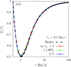
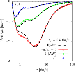
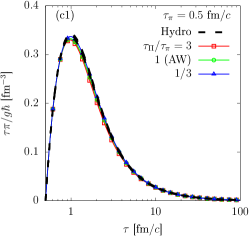
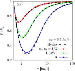
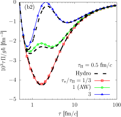
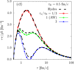
Figure 1: Time evolution of (a1,a2) $P_{l}/P_{\perp}$, (b1,b2), $\tau\Pi/g\hbar$, and (c1,c2) $\tau\pi/g\hbar$ in a $0+1$-dimensional Bjorken expansion of an ideal gas with vanishing chemical potential and rest mass $m_{0}=1\ {\rm GeV}/c^{2}$. In panels (a1)–(c1), $\tau_{\pi}=0.5\ {\rm fm}/c$ is fixed and $\tau_{\Pi}/\tau_{\pi}$ is changed via the Shakhov collision term. In panels (a2)–(c2), $\tau_{\Pi}=0.5\ {\rm fm}/c$ and $\tau_{\pi}/\tau_{\Pi}$ is varied. The value $\tau_{\Pi}/\tau_{\pi}=1$ corresponds to the AW model (green line), while $\tau_{\Pi}/\tau_{\pi}=3$ and $1/3$ are shown with red and blue lines, respectively. The dashed black lines are the solutions of second-order fluid dynamics in Eqs. (36,37).

5 Example I: Bjorken flow

We consider the $(0+1)$–dimensional boost-invariant Bjorken expansion [45] of a classical ($a\equiv 0$) ideal gas of massive particles. Enforcing $\mu\equiv\nabla^{\mu}\alpha=0$ leads to $f_{0{\mathbf{k}}}=\exp(-\beta E_{\mathbf{k}})$ and $\partial_{\mu}N^{\mu}\neq 0$, with vanishing diffusion current. This leaves only two independent transport coefficients: $\zeta$ and $\eta$. Now, replacing $\tau_{R}=\tau_{\Pi}$ and $J_{42}=(e+P)/\beta^{2}$ the Shakhov distribution (22) reduces to

$$f_{{\rm S}{\mathbf{k}}}=f_{0{\mathbf{k}}}\left[1+\frac{\beta^{2}k_{\langle\mu}k_{\nu\rangle}\pi^{\mu\nu}}{2(e+P)}\left(1-\frac{\tau_{\Pi}}{\tau_{\pi}}\right)\right].$$ (34)

In the $(\tau,x,y,\eta_{s})$ coordinates, with proper-time $\tau=\sqrt{t^{2}-z^{2}}$ and space-time rapidity $\eta_{s}={\rm artanh}(z/t)$, the energy-momentum tensor is diagonal, $T^{\mu\nu}={\rm diag}(e,P_{\perp},P_{\perp},\tau^{-2}P_{l})$. The transverse $P_{\perp}$ and longitudinal $P_{l}$ pressure components are related to the pressure $P$, the bulk pressure $\Pi$, and the shear-stress tensor component $\pi=\pi^{\eta_{s}}_{\eta_{s}}$ via

$$P_{\perp}=P+\Pi+\frac{\pi}{2},\quad P_{l}=P+\Pi-\pi.$$ (35)

In the Shakhov model, the time evolution of $P$, $\Pi$ and $\pi$ is obtained by directly solving the Boltzmann equation $k^{\mu}\partial_{\mu}f=C_{\rm S}[f]$, as described in the Supplementary Material [44].

For direct comparison to the kinetic model, we also compute the fluid-dynamical evolution, where the energy conservation equation $u_{\nu}\partial_{\mu}T^{\mu\nu}=0$ reduces to

$$\tau\frac{de}{d\tau}+e+P_{l}=0,$$ (36)

and it is closed by the following relaxation equations [37, 46]

$$\tau\frac{d\Pi}{d\tau}+\left(\frac{\delta_{\Pi\Pi}}{\tau_{\Pi}}+\frac{\tau}{\tau_{\Pi}}\right)\Pi-\frac{\lambda_{\Pi\pi}}{\tau_{\Pi}}\pi =-\frac{\zeta}{\tau_{\Pi}},$$ (37a)

$$\tau\frac{d\pi}{d\tau}+\left(\frac{\delta_{\pi\pi}}{\tau_{\pi}}+\frac{\tau_{\pi\pi}}{3\tau_{\pi}}+\frac{\tau}{\tau_{\pi}}\right)\pi-\frac{2\lambda_{\pi\Pi}}{3\tau_{\pi}}\Pi =\frac{4\eta}{3\tau_{\pi}},$$ (37b)

with the first-order transport coefficients given by

$$\zeta=\tau_{\Pi}\frac{m_{0}^{2}\beta}{3}\left(\frac{J_{31}}{J_{30}}J_{10}-J_{11}\right),\quad\eta=\tau_{\pi}\beta J_{32}.$$ (38)

The second-order transport coefficients $\delta_{\Pi\Pi}$, $\lambda_{\Pi\pi}$, $\delta_{\pi\pi}$, $\tau_{\pi\pi}$, and $\lambda_{\pi\Pi}$ are derived from the Shakhov collision term, as shown in the Supplementary Material [44].

In order to validate the kinetic Shakhov model, we performed two sets of simulations with particles of mass $m_{0}=1\ {\rm GeV}/c^{2}$. At initial time $\tau_{0}=0.5\ {\rm fm}/c$ and initial temperature $\beta_{0}^{-1}=0.5\ {\rm GeV}$, we set $f_{{\mathbf{k}}}(\tau_{0})=\exp(-\beta_{0}E_{\mathbf{k}})$. The results obtained using the AW model with $\tau_{\pi}=\tau_{\Pi}=\tau_{R}=0.5\ {\rm fm}/c$, leading to $4\pi\eta/s\simeq 2.6$ at the initial time, are used as reference. The solutions of the corresponding second-order fluid-dynamical equations (36)–(37) are shown in Fig. 1 with dashed black lines.

Panels (a1)–(c1) of Fig. 1 show the results where $\tau_{\pi}=0.5\ {\rm fm}/c$ is fixed, while $\tau_{\Pi}=\tau_{R}$ is varied. The red, green and blue lines with symbols correspond to the kinetic equation with $\tau_{\Pi}/\tau_{\pi}=3$, $1$ and $1/3$, respectively. Panels (a1) and (c1) show that the evolution of $P_{l}/P_{\perp}$ and $\pi$ remains independent of $\tau_{\Pi}$. Panel (b1) shows that the amplitude of $\Pi$ scales roughly with the ratio $\tau_{\Pi}/\tau_{\pi}$. Panels (a2)–(c2) depict the results for fixed $\tau_{\Pi}\equiv\tau_{R}=0.5\ {\rm fm}/c$ and variable $\tau_{\pi}$. During an initial period of time, (b2) indicates a non-linear dependence of $\Pi$ on $\tau_{\pi}$. However, at late times, all curves converge towards an asymptotic solution governed by the value of $\tau_{\Pi}$. Panels (a2) and (c2) display the expected dependence of $P_{l}/P_{\perp}$ and $\pi$ on $\tau_{\pi}$, with a larger dip and a slower approach to equilibrium, $P_{l}/P_{\perp}=1$ and $\pi=0$, for larger values of $\tau_{\pi}$. The small discrepancies observable in Fig. 1 between the kinetic and fluid-dynamical results are expected due to the large values of the relaxation times and their associated viscosities [46, 47, 48]. The results at smaller/larger viscosities are in better/worse agreement.

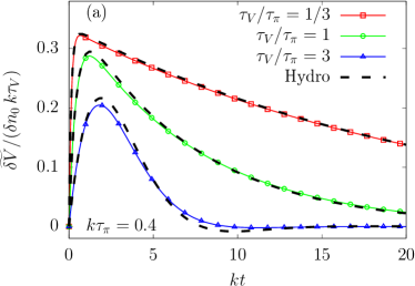
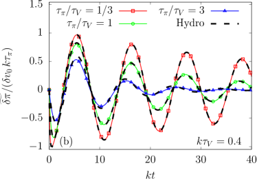
Figure 2: Time evolution of the amplitudes (a) $\widetilde{\delta V}/(\delta n_{0}k\tau_{V})$ for fixed $k\tau_{\pi}=0.4$ and variable $\tau_{V}/\tau_{\pi}$; and (b) $\widetilde{\delta\pi}/(\delta v_{0}k\tau_{\pi})$ for fixed $k\tau_{V}=0.4$ and variable $\tau_{\pi}/\tau_{V}$, in the context of the propagation of longitudinal waves of wave number $k=2\pi/L$ through an ultrarelativistic gas. The curves with $\tau_{V}=\tau_{\pi}$ correspond to the AW model. The dashed black lines are the solutions of second-order fluid-dynamics. The initial amplitudes were set to $\delta n_{0}/n_{0}=\delta v_{0}=10^{-3}$.

6 Example II: Longitudinal waves

We now consider sound waves propagating through an ultrarelativistic, classical ideal gas at rest, with temperature $\beta_{0}^{-1}=0.6\ {\rm GeV}$ and $\alpha_{0}=0$. Since $\zeta=0$ when $m_{0}=0$, we are left with only two transport coefficients: $\kappa$ and $\eta$. Setting $\tau_{\pi}=\tau_{R}$ and $\tau_{V}\neq\tau_{R}$ in Eq. (22) and using $J_{nq}=I_{nq}=P\beta^{2-n}(n+1)!/[2(2q+1)!!]$ leads to

$$f_{{\rm S}{\mathbf{k}}}=f_{0{\mathbf{k}}}\left[1+\frac{k_{\langle\mu\rangle}V^{\mu}}{P}(\beta E_{\mathbf{k}}-5)\left(1-\frac{\tau_{\pi}}{\tau_{V}}\right)\right],$$ (39)

where $f_{0{\mathbf{k}}}=e^{\alpha-\beta E_{\mathbf{k}}}$. At the initial time, the system is in equilibrium and the density $n=n_{0}+\delta n$ and velocity $u^{z}=\delta v$ are perturbed via $\delta n=\delta n_{0}\cos(kz)$ and $\delta v=\delta v_{0}\sin(kz)$, while the pressure is unperturbed, $P=P_{0}=n_{0}T_{0}$. Here, $k=2\pi/L$ and $L=6.4\ {\rm fm}$, while $\delta n_{0}/n_{0}=\delta v_{0}/c=10^{-3}$. We then track the time evolution of the amplitudes $\widetilde{\delta\pi}$ and $\widetilde{\delta V}$, computed as

$$\widetilde{\delta V}=\frac{2}{L}\int_{0}^{L}dz\,\delta V\,\cos(kz),\quad\widetilde{\delta\pi}=\frac{2}{L}\int_{0}^{L}dz\,\delta\pi\,\sin(kz),$$ (40)

where $\delta V=V^{z}$ and $\delta\pi\simeq\pi^{zz}$ correspond to the diffusion current and shear-stress tensor, respectively. For more details, see Sec. V of Ref. [42].

We now compare the numerical solution of the full Shakhov model described by Eqs. (12) and (39), obtained as described in the Supplementary Material [44], with the solution of the linearized second-order fluid dynamical equations, computed using the methods of Refs. [15, 42]. Panel (a) shows the ratio $\widetilde{\delta V}/(\delta n_{0}k\tau_{V})$ for three values of $\tau_{V}/\tau_{\pi}$, with $k\tau_{\pi}=0.4$ fixed, such that $4\pi\eta/s\simeq 3.11$. It can be seen that the amplitude of $\widetilde{\delta V}$ and the damping exponent scale almost linearly with $\tau_{V}$. Similarly, for the $\widetilde{\delta\pi}/(\delta v_{0}k\tau_{\pi})$ ratio shown in panel (b), we varied $\tau_{\pi}/\tau_{V}$ while keeping $k\tau_{V}=0.4$ fixed. This panel shows that the damping exponent of $\widetilde{\delta\pi}$ is proportional to $\tau_{\pi}$. Small discrepancies between the kinetic and fluid-dynamical results when $\tau_{V}/\tau_{\pi}=3$ in panel (a) or $\tau_{\pi}/\tau_{V}=3$ in panel (b) are due to the departure from the domain of applicability of second-order fluid dynamics [15].

7 Conclusion

In this paper, we introduced the relativistic Shakhov-type model as an extension of the Anderson-Witting RTA with momentum-independent relaxation time. This model introduces new and independently-adjustable first-order transport coefficients/relaxation times for the bulk viscous pressure, diffusion current, and shear-stress tensor. Although here our primary focus was on the first-order transport coefficients, the Shakhov model can be systematically extended [49] to control all transport coefficients of second-order fluid dynamics.

This more general kinetic equation makes it possible to study different values or parameterizations of the first-order transport coefficients in various phenomena such as the baryon diffusion or the effect of bulk and shear viscosities similarly as in the state of the art second-order fluid dynamical simulations. Therefore, the present work significantly extends the applicability of kinetic RTA models to describe systems relevant in high-energy heavy-ion collisions.

SUPPLEMENTARY
MATERIAL

This supplementary material is structured in three sections. Section SM-1 discusses the second-order transport coefficients from the Shakhov model. Section SM-2 presents the entropy production, while Section SM-3 summarizes the details of the numerical scheme used to solve the Shakhov model equation.

SM-1 Second-order transport coefficients of the relativistic Shakhov model

In this section we employ the method of moments of Refs. [35, 37] to derive the first- and second-order transport coefficients corresponding to the relativistic Shakhov model. These transport coefficients arise at first- and second-order with respect to the Knudsen number Kn, being the ratio of the particle mean free path and a characteristic macroscopic scale, and the inverse Reynolds number $\mathrm{Re}^{-1}$, being the ratio of an out-of-equilibrium and a local-equilibrium macroscopic field.

Irreducible moments and orthogonal basis.– The irreducible moments from Eq. (6) are expressed as [35],

$$\delta f_{\mathbf{k}}=f_{0\mathbf{k}}\tilde{f}_{0{\mathbf{k}}}\sum_{\ell=0}^{\infty}\sum_{n=0}^{N_{\ell}}\rho_{n}^{\mu_{1}\cdots\mu_{\ell}}k_{\left\langle\mu_{1}\right.}\cdots k_{\left.\mu_{\ell}\right\rangle}\mathcal{H}_{\mathbf{k}n}^{(\ell)},$$ (SM-1)

where $N_{\ell}\rightarrow\infty$ is an expansion order. The functions $\mathcal{H}^{(\ell)}_{{\mathbf{k}}n}$ are polynomials of order $N_{\ell}$ with respect to $E_{\mathbf{k}}$, defined in full generality in Eq. (29) of Ref. [35], and are constructed such that Eq. (6) is satisfied for $0\leq r\leq N_{\ell}$. We remark that, while Eq. (SM-1) employs an irreducible basis, the expansion does not account explicitly for the negative-order moments $\rho_{r}^{\mu_{1}\cdots\mu_{\ell}}$ with $r<0$, but these must be reconstructed from those with $0\leq r\leq N_{\ell}$ in a manner which becomes exact only in the limit $N_{\ell}\rightarrow\infty$. The simple structure of the RTA model allows to circumvent such construction in Eq. (SM-1) by employing a basis-free approach, as discussed in Ref. [42].

We note that the functions $\mathcal{H}^{(\ell)}_{{\mathbf{k}}n}$, related to the representation of $\delta f_{\mathbf{k}}$ are also useful in the context of the Shakhov model. However, for the Shakhov distribution, $N_{\ell}$ is not the expansion order of $\delta f_{\mathbf{k}}$, but the order of the $\mathcal{H}^{(\ell)}_{{\mathbf{k}}0}$ polynomials satisfying the constraints in Eq. (20), namely $N_{0}=2$, $N_{1}=1$, and $N_{2}=0$.

The Shakhov collision term from Eq. (12) is

$$C^{\mu_{1}\cdots\mu_{\ell}}_{r-1}=-\frac{1}{\tau_{R}}\rho^{\mu_{1}\cdots\mu_{\ell}}_{r}+\frac{1}{\tau_{R}}\rho^{\mu_{1}\cdots\mu_{\ell}}_{{\rm S},r},$$ (SM-2)

where the second term involves the irreducible moments of $\delta f_{{\rm S}{\mathbf{k}}}=f_{0{\mathbf{k}}}\tilde{f}_{0{\mathbf{k}}}\mathbb{S}_{\mathbf{k}}$ defined in Eq. (14). Now, using the Shakhov distribution from Eq. (22) leads to

$$\rho_{{\rm S},r}=-\frac{3\Pi}{m_{0}^{2}}\left(1-\frac{\tau_{R}}{\tau_{\Pi}}\right)\mathcal{F}^{(0)}_{-r,0},\quad\rho_{{\rm S},r}^{\mu}=V^{\mu}\left(1-\frac{\tau_{R}}{\tau_{V}}\right)\mathcal{F}^{(1)}_{-r,0},$$

$$\rho_{{\rm S},r}^{\mu\nu}=\pi^{\mu\nu}\left(1-\frac{\tau_{R}}{\tau_{\pi}}\right)\mathcal{F}^{(2)}_{-r,0},$$ (SM-3)

while the higher-rank moments are set to vanish, i.e., $\rho_{{\rm S},r}^{\mu_{1}\cdots\mu_{\ell}}=0$ with $\ell>2$. Now using Eq. (28) for polynomial orders $N_{0}=2$, $N_{1}=1$, and $N_{2}=0$, ensures that $\mathcal{F}^{(0)}_{0,0}=\mathcal{F}^{(1)}_{0,0}=\mathcal{F}^{(2)}_{0,0}=1$ and $\mathcal{F}^{(0)}_{-1,0}=\mathcal{F}^{(0)}_{-2,0}=\mathcal{F}^{(1)}_{-1,0}=0$.

The second-order transport coefficients also require the knowledge of various other moments $\rho^{\mu_{1}\cdots\mu_{\ell}}_{r\neq 0}$. Here we recall the first-order approximation to such irreducible moments in the so-called basis-free approach of Ref. [42]:

$$\rho_{r\neq 0}\simeq-\frac{3}{m_{0}^{2}}\mathcal{R}^{(0)}_{r0}\Pi,\quad\rho^{\mu}_{r\neq 0}\simeq\mathcal{R}^{(1)}_{r0}V^{\mu},\quad\rho^{\mu\nu}_{r\neq 0}\simeq\mathcal{R}^{(2)}_{r0}\pi^{\mu\nu},$$ (SM-4)

where

$$\mathcal{R}^{(0)}_{r0}=\frac{\zeta_{r}}{\zeta}\,,\quad\mathcal{R}^{(1)}_{r0}=\frac{\kappa_{r}}{\kappa}\,,\quad\mathcal{R}^{(2)}_{r0}=\frac{\eta_{r}}{\eta}\,.$$ (SM-5)

Now, substituting the expressions for the first-order transport coefficients from Eqs. (31) into Eq. (SM-5) gives

$$\mathcal{R}^{(\ell)}_{-r,0}=\frac{\tau_{R}}{\tau_{\rm S}^{(\ell)}}\frac{\alpha^{(\ell)}_{-r}}{\alpha^{(\ell)}_{0}}+\left(1-\frac{\tau_{R}}{\tau_{\rm S}^{(\ell)}}\right)\mathcal{F}^{(0)}_{r0}.$$ (SM-6)

Using these results, the relaxation times can be computed using Eqs. (38) of Ref. [54]:

$$\tau_{\Pi}=\sum_{r\neq 1,2}\tau^{(0)}_{0r}\mathcal{R}^{(0)}_{r0},\quad\tau_{V}=\sum_{r\neq 1}\tau^{(1)}_{0r}\mathcal{R}^{(1)}_{r0},\quad\tau_{\pi}=\sum_{r}\tau^{(2)}_{0r}\mathcal{R}^{(2)}_{r0}.$$ (SM-7)

Recalling the expression for $\tau^{(\ell)}_{nr}$ from Eqs. (29) together with Eq. (SM-6), the above definitions leads to $\tau_{\Pi}=\tau^{(0)}_{\rm S}$, $\tau_{V}=\tau^{(1)}_{\rm S}$, and $\tau_{\pi}=\tau^{(2)}_{\rm S}$, as expected.

As discussed in Ref. [42], the second-order transport coefficients involve only the coefficients $\mathcal{R}^{(\ell)}_{-1,0}$ and $\mathcal{R}^{(\ell)}_{-2,0}$. These coefficients also require the expressions for $\mathcal{F}^{(\ell)}_{r0}$ computed using the functions $\mathcal{H}^{(\ell)}_{{\mathbf{k}}0}$ in Eq. (23), as shown below:

$$\mathcal{F}^{(0)}_{r0}=\frac{J_{-r,0}G_{33}-J_{1-r,0}G_{23}+J_{2-r,0}G_{22}}{J_{00}G_{33}-J_{10}G_{23}+J_{20}G_{22}},$$

$$\mathcal{F}^{(1)}_{r0}=\frac{J_{2-r,1}J_{41}-J_{3-r,1}J_{31}}{J_{21}J_{41}-J_{31}^{2}},\quad\mathcal{F}^{(2)}_{r0}=\frac{J_{4-r,2}}{J_{42}}.$$ (SM-8)

Equations of motion.– The relaxation equations for $\Pi=-m^{2}_{0}\rho_{0}/3$, $V^{\mu}=\rho_{0}^{\mu}$, and $\pi^{\mu\nu}=\rho_{0}^{\mu\nu}$ are obtained by setting $n=0$ in Eqs. (30). Up to second order with respect to ${\rm Kn}$ and ${\rm Re}^{-1}$, these equations read, see Eqs. (88-93) in Ref. [42],

$$\tau_{\Pi}\dot{\Pi}+\Pi=-\zeta\theta-\ell_{\Pi V}\nabla_{\mu}V^{\mu}-\tau_{\Pi V}V_{\mu}\dot{u}^{\mu}-\delta_{\Pi\Pi}\Pi\theta$$

$$\hskip 30.0pt-\lambda_{\Pi V}V_{\mu}\nabla^{\mu}\alpha+\lambda_{\Pi\pi}\pi^{\mu\nu}\sigma_{\mu\nu},$$ (SM-9a)

$$\tau_{V}\dot{V}^{\langle\mu\rangle}+V^{\mu}=\kappa\nabla^{\mu}\alpha-\tau_{V}V_{\nu}\omega^{\nu\mu}-\delta_{VV}V^{\mu}\theta$$

$$\hskip 30.0pt-\ell_{V\Pi}\nabla^{\mu}\Pi+\ell_{V\pi}\Delta^{\mu\nu}\nabla_{\lambda}\pi^{\lambda}_{\nu}+\tau_{V\Pi}\Pi\dot{u}^{\mu}-\tau_{V\pi}\pi^{\mu\nu}\dot{u}_{\nu}$$

$$\hskip 30.0pt-\lambda_{VV}V_{\nu}\sigma^{\mu\nu}+\lambda_{V\Pi}\Pi\nabla^{\mu}\alpha-\lambda_{V\pi}\pi^{\mu\nu}\nabla_{\nu}\alpha,$$ (SM-9b)

$$\tau_{\pi}\dot{\pi}^{\langle\mu\nu\rangle}+\pi^{\mu\nu}=2\eta\sigma^{\mu\nu}+2\tau_{\pi}\pi_{\lambda}^{\langle\mu}\omega^{\nu\rangle\lambda}-\delta_{\pi\pi}\pi^{\mu\nu}\theta$$

$$\hskip 30.0pt-\tau_{\pi\pi}\pi^{\lambda\langle\mu}\sigma^{\nu\rangle}_{\lambda}+\lambda_{\pi\Pi}\Pi\sigma^{\mu\nu}-\tau_{\pi V}V^{\langle\nu}\dot{u}^{\mu\rangle}$$

$$\hskip 30.0pt+\ell_{\pi V}\nabla^{\langle\mu}V^{\nu\rangle}+\lambda_{\pi V}V^{\langle\mu}\nabla^{\nu\rangle}\alpha.$$ (SM-9c)

Shakhov model for the Bjorken flow.– In the case of the Bjorken expansion, we considered a massive ideal gas such that $\alpha^{(0)}_{r}$ is given by Eq. (10). The first-order transport coefficients $\zeta$ and $\eta$ are listed in Eqs. (38). The second-order transport coefficients appearing in Eq. (37) are listed here from Ref. [37]:

$$\delta_{\Pi\Pi} =\tau_{\Pi}\left(\frac{2}{3}+\frac{m_{0}^{2}}{3}\frac{J_{10}}{J_{30}}+\frac{m_{0}^{2}}{3}{\mathcal{R}}^{(0)}_{-2,0}\right),$$ (SM-10)

$$\lambda_{\Pi\pi} =\tau_{\Pi}\frac{m_{0}^{2}}{3}\left(\frac{J_{10}}{J_{30}}+{\mathcal{R}}^{(2)}_{-2,0}\right),\quad\delta_{\pi\pi}=\tau_{\pi}\left(\frac{4}{3}+\frac{m_{0}^{2}}{3}\mathcal{R}^{(2)}_{-2,0}\right),$$

$$\tau_{\pi\pi} =\tau_{\pi}\left(\frac{10}{7}+\frac{4m_{0}^{2}}{7}\mathcal{R}^{(2)}_{-2,0}\right),\quad\lambda_{\pi\Pi}=\tau_{\pi}\left(\frac{6}{5}+\frac{2m_{0}^{2}}{5}\mathcal{R}^{(0)}_{-2,0}\right).$$

Since the Shakhov distribution employed in Eq. (34) uses $\tau_{\Pi}=\tau_{R}$, the coefficients $\mathcal{R}^{(0)}_{-r,0}$ reduce to their corresponding values for the AW model, namely

$$\mathcal{R}^{(0)}_{-r,0}\equiv\frac{\alpha^{(0)}_{-r}}{\alpha^{(0)}_{0}}=\frac{J_{1-r,0}J_{31}-J_{1-r,1}J_{30}}{J_{10}J_{31}-J_{11}J_{30}},$$ (SM-11)

where Eq. (10) was employed to replace $\alpha^{(0)}_{r}$. On the other hand, $\mathcal{R}^{(2)}_{-r,0}$ becomes

$$\mathcal{R}^{(2)}_{-r,0}=\frac{\tau_{\Pi}}{\tau_{\pi}}\frac{J_{3-r,2}}{J_{32}}+\left(1-\frac{\tau_{\Pi}}{\tau_{\pi}}\right)\frac{J_{4-r,2}}{J_{42}},$$ (SM-12)

which in the limit of $\tau_{\Pi}=\tau_{\pi}$ recovers the analogous coefficient appearing in the AW model, $\alpha^{(2)}_{-r}/\alpha^{(2)}_{0}=J_{3-r,2}/J_{32}$. Therefore, the transport coefficients $\lambda_{\Pi\pi}$, $\delta_{\pi\pi}$, and $\tau_{\pi\pi}$ involving $\mathcal{R}^{(2)}_{-2,0}$ are modified with respect to their AW expressions, while $\delta_{\Pi\Pi}$ and $\lambda_{\pi\Pi}$ remain unchanged.

Shakhov model for longitudinal waves.– In the case of the longitudinal waves concerning an ultrarelativistic classical ideal gas, we have

$$J_{nq} \equiv I_{nq}=\frac{P\beta^{2-n}(n+1)!}{2(2q+1)!!}, P =\frac{ge^{\alpha}}{\pi^{2}\beta^{4}},$$

$$\alpha^{(1)}_{r} =\frac{P(r+2)!(1-r)}{24\beta^{r-1}}, \alpha^{(2)}_{r} =\frac{P(r+4)!}{30\beta^{r}}.$$ (SM-13)

The transport coefficients from Eq. (SM-9b) reduce to [42]:

$$\delta_{VV}=\tau_{V},\quad\ell_{V\pi}=\frac{\tau_{V}}{h}\!\left(1-h\mathcal{R}^{(2)}_{-1,0}\right),\quad\tau_{V\pi}=\frac{\tau_{V}}{h}\!\left(1-h\frac{\partial\mathcal{R}^{(2)}_{-1,0}}{\partial\ln\beta}\right),$$

$$\lambda_{VV}=\frac{3}{5}\tau_{V},\quad\lambda_{V\pi}=\tau_{V}\left(\frac{\partial\mathcal{R}^{(2)}_{-1,0}}{\partial\alpha}+\frac{1}{h}\frac{\partial\mathcal{R}^{(2)}_{-1,0}}{\partial\beta}\right),$$ (SM-14)

where $h=(e+P)/n$ is the enthalpy per particle. Noting that

$$\mathcal{F}^{(2)}_{10}=\frac{\beta}{5},\quad\mathcal{R}^{(2)}_{-1,0}=\frac{\beta}{4}\left(1+\frac{\tau_{R}-\tau_{\pi}}{5\tau_{\pi}}\right),$$ (SM-15)

the Shakhov model alters only the following coefficients:

$$\ell_{V\pi}\equiv\tau_{V\pi} =\frac{\beta}{20}\left(1-\frac{\tau_{R}}{\tau_{\pi}}\right)\tau_{V},$$ (SM-16a)

$$\lambda_{V\pi} =\frac{\beta}{16}\left(1+\frac{\tau_{R}-\tau_{\pi}}{5\tau_{\pi}}\right)\tau_{V}.$$ (SM-16b)

Similarly, the coefficients appearing in Eq. (SM-9c) are

$$\delta_{\pi\pi} =\frac{4}{3}\tau_{\pi}, \tau_{\pi\pi} =\frac{10}{7}\tau_{\pi}, \ell_{\pi V} =\tau_{\pi V}=\lambda_{\pi V}=0,$$ (SM-16c)

while $\kappa=\frac{\beta P}{12}\tau_{V}$ and $\eta=\frac{4P}{5}\tau_{\pi}$. The Shakhov collision term considered in Eq. (39) employs $\tau_{\pi}=\tau_{R}$, hence the dependence on $\tau_{\pi}$ disappears in Eqs. (SM-16) and all transport coefficients reduce to the AW ones (with $\tau_{R}$ replaced by $\tau_{V}$ or $\tau_{\pi}$, as appropriate), see for comparison Eqs. (168) and (169) in Ref. [42].

SM-2 Entropy production

We now discuss the thermodynamic consistency of the Shakhov model by considering the entropy production

$$\partial_{\mu}S^{\mu}=-\int dK\,C_{\rm S}[f]\ln(f_{\mathbf{k}}/\tilde{f}_{\mathbf{k}}),$$ (SM-17)

where $S^{\mu}=-\int dK\,k^{\mu}(f_{\mathbf{k}}\ln f_{\mathbf{k}}+a\tilde{f}_{\mathbf{k}}\ln\tilde{f}_{\mathbf{k}})$ is the entropy four-current. As originally pointed out by Shakhov [17], asserting the sign of $\partial_{\mu}S^{\mu}$ for arbitrary distributions $f_{\mathbf{k}}$ is difficult, but if the fluid is not far from equilibrium, quadratic terms in $\delta f_{\mathbf{k}}$ or $\delta f_{{\rm S}{\mathbf{k}}}$ can be neglected and the logarithm in Eq. (SM-17) can be approximated as:

$$\ln\frac{f_{\mathbf{k}}}{\tilde{f}_{\mathbf{k}}}=\ln\frac{f_{0{\mathbf{k}}}(1+\tilde{f}_{0{\mathbf{k}}}\phi_{\mathbf{k}})}{\tilde{f}_{0{\mathbf{k}}}(1-af_{0{\mathbf{k}}}\phi_{\mathbf{k}})}\simeq\ln\frac{f_{0{\mathbf{k}}}}{\tilde{f}_{0{\mathbf{k}}}}+\phi_{\mathbf{k}}+O(\phi_{\mathbf{k}}^{2}),$$ (SM-18)

where $\phi_{\mathbf{k}}=\delta f_{\mathbf{k}}/(f_{0{\mathbf{k}}}\tilde{f}_{0{\mathbf{k}}})$. Thus, Eq. (SM-17) becomes

$$\partial_{\mu}S^{\mu}\simeq\frac{1}{\tau_{R}}\int dKE_{\mathbf{k}}(\delta f_{\mathbf{k}}-\delta f_{{\rm S}{\mathbf{k}}})\ln\frac{f_{0{\mathbf{k}}}}{\tilde{f}_{0{\mathbf{k}}}}\\ +\frac{1}{\tau_{R}}\int dKE_{\mathbf{k}}\delta f_{\mathbf{k}}\left(\phi_{\mathbf{k}}-\mathbb{S}_{\mathbf{k}}\right),$$ (SM-19)

where on the second line, we have used the relation $(\delta f_{\mathbf{k}}-\delta f_{{\rm S}{\mathbf{k}}})\phi_{\mathbf{k}}=\delta f_{\mathbf{k}}(\phi_{\mathbf{k}}-\mathbb{S}_{\mathbf{k}})$ with $\mathbb{S}_{\mathbf{k}}=\delta f_{{\rm S}{\mathbf{k}}}/f_{0{\mathbf{k}}}\widetilde{f}_{0{\mathbf{k}}}$. Since $\ln(f_{0{\mathbf{k}}}/\tilde{f}_{0{\mathbf{k}}})=\alpha-\beta E_{\mathbf{k}}$, the first term on the right-hand side of the equation vanishes due to the matching conditions in Eq. (19). The second term can be estimated using Eq. (13), leading to

$$\phi_{\mathbf{k}}-\mathbb{S}_{\mathbf{k}}\simeq-\frac{\tau_{R}}{E_{\mathbf{k}}}k^{\mu}\partial_{\mu}(\alpha-\beta E_{\mathbf{k}}),$$ (SM-20)

and with Eq. (17) confirms the second law of thermodynamics,

$$\partial_{\mu}S^{\mu}\simeq\frac{\beta}{\zeta}\Pi^{2}-\frac{1}{\kappa}V_{\mu}V^{\mu}+\frac{\beta}{2\eta}\pi_{\mu\nu}\pi^{\mu\nu}\geq 0.$$ (SM-21)

SM-3 Numerical method for the Shakhov model

To solve the Shakhov kinetic model $k^{\mu}\partial_{\mu}f_{\mathbf{k}}=C_{\rm S}[f]$, we employ a discrete velocity method inspired by the Relativistic Lattice Boltzmann algorithm of Refs. [16, 55, 56, 57, 58]. We consider the rapidity-based moments of $f_{\mathbf{k}}$ introduced in Ref. [37], which eliminates two out of the three dimensions of the momentum space for the particular case of the $(1+1)$-dimensional longitudinal waves SM-3.1, and the $(0+1)$-dimensional boost invariant expansion SM-3.2, respectively.

SM-3.1 Longitudinal wave damping problem

In the application of Sec. 6, the fluid is homogeneous with respect to the $x$ and $y$ directions. Parameterizing the momentum space using $(m_{\perp},\varphi_{\perp},v^{z})$ as in Ref. [37],

$$\begin{pmatrix}k^{t}\\ k^{z}\end{pmatrix}=\frac{m_{\perp}}{\sqrt{1-v_{z}^{2}}}\begin{pmatrix}1\\ v^{z}\end{pmatrix},\quad\begin{pmatrix}k^{x}\\ k^{y}\end{pmatrix}=\sqrt{m_{\perp}^{2}-m_{0}^{2}}\begin{pmatrix}\cos\varphi_{\perp}\\ \sin\varphi_{\perp}\end{pmatrix},$$ (SM-22)

the Boltzmann equation with the Shakhov model for the collision term reduces to

$$\partial_{t}f_{\mathbf{k}}+v^{z}\partial_{z}f_{\mathbf{k}}=-\frac{u\cdot v}{\tau_{R}}(f_{\mathbf{k}}-f_{{\rm S}{\mathbf{k}}}),$$ (SM-23)

where $v^{\mu}=k^{\mu}/k^{t}$ and $u\cdot v=\gamma(1-\beta^{z}v^{z})$, with $\beta^{z}$ being the fluid three-velocity along the $z$ direction and $\gamma=1/\sqrt{1-\beta_{z}^{2}}$. Introducing the rapidity-based moments [37]

$$F_{n}=\frac{g}{(2\pi)^{3}}\int_{0}^{2\pi}d\varphi_{\perp}\int_{m_{0}}^{\infty}\frac{dm_{\perp}\,m_{\perp}^{n+1}}{(1-v_{z}^{2})^{(n+2)/2}}f_{\mathbf{k}},$$ (SM-24)

Eq. (SM-23) becomes

$$\partial_{t}F_{n}+v^{z}\partial_{z}F_{n}=-\frac{u\cdot v}{\tau_{R}}(F_{n}-F^{\rm S}_{n}).$$ (SM-25)

It can be shown [49] that the macroscopic quantities $N^{t}$, $N^{z}$, $T^{tt}$, $T^{tz}$ and $T^{zz}$ can be obtained from $F_{1}$ and $F_{2}$ via

$$\begin{pmatrix}N^{t}\\ N^{z}\end{pmatrix}=\int_{-1}^{1}dv^{z}\begin{pmatrix}1\\ v^{z}\end{pmatrix}F_{1},\quad\begin{pmatrix}T^{tt}\\ T^{tz}\\ T^{zz}\end{pmatrix}=\int_{-1}^{1}dv^{z}\begin{pmatrix}1\\ v^{z}\\ v_{z}^{2}\end{pmatrix}F_{2}.$$ (SM-26)

For the case of massless particles considered in Sec. 6, $T^{\mu}{}_{\mu}=0$, such that $T^{xx}=T^{yy}=T^{tt}-T^{zz}$. From the above, it is clear that the time evolution of both $N^{\mu}$ and $T^{\mu\nu}$ is fully determined by the functions $F_{1}$ and $F_{2}$. In order to solve Eq. (SM-25), the functions $F^{\rm S}_{n}$ must be obtained by integrating Eq. (39), yielding:

$$F^{\rm S}_{1}=\frac{n}{2(u\cdot v)^{3}}-\frac{3V(\beta^{z}-v^{z})}{2(u\cdot v)^{4}}\left(1-\frac{\tau_{\pi}}{\tau_{V}}\right),\quad F^{\rm S}_{2}=\frac{3P}{2(u\cdot v)^{4}}.$$ (SM-27)

The time discretization is performed using equal time steps $\delta t=10^{-3}\,{\rm fm}/c$ and the time stepping is performed using the third-order total variation diminishing (TVD) Runge-Kutta scheme [59, 60]. The spatial domain $[-L/2,L/2]$ is discretized using $S=100$ cells of size $\delta s=L/S$, centred on $z_{s}=(s-\frac{1}{2})\delta s-\frac{L}{2}$, $1\leq s\leq S$. The spatial derivative $v^{z}\partial_{z}F_{n}$ is approximated using finite differences:

$$\left(v_{z}\frac{\partial F_{n}}{\partial z}\right)_{s}=\frac{\mathbf{F}_{n;s+1/2}-\mathbf{F}_{n;s-1/2}}{\delta s},$$ (SM-28)

where $\mathbf{F}_{n;s+1/2}$ represents the flux at the interface between cells $s$ and $s+1$. For definiteness, we compute this flux using the upwind-biased fifth-order weighted essentially non-oscillatory (WENO-5) scheme introduced in Ref. [61, 62]. Finally, the $v^{z}$ momentum space coordinate is discretized via the Gauss-Legendre quadrature with $K=20$ points, such that $P_{K}(v^{z}_{j})=0$, with $1\leq j\leq K$ and $P_{K}(z)$ being the Legendre polynomial of order $K$. Then, integrals with respect to $v^{z}$ of a function $g(v^{z})$ are approximated via

$$\int_{-1}^{1}dv^{z}\,g(v^{z})\simeq\sum_{j=1}^{K}g_{j},\qquad g_{j}\equiv w_{j}g(v^{z}_{j}),$$ (SM-29)

with $w_{j}$ being the Gauss-Legendre quadrature weights [63].

SM-3.2 Algorithm for the Bjorken expansion

The algorithm for the Bjorken expansion is identical to that described in Ref. [37], hence we only recall the main method here. The spatial rapidity is $\eta_{s}={\rm artanh}(z/t)$, and the parametrization of the momentum space is as in Eq. (SM-22), with $(k^{t},k^{z})$ replaced by $(k^{\tau},\tau k^{\eta_{s}})$, where

$$k^{\tau}=\frac{1}{\tau}(tk^{t}-zk^{z}),\quad\tau k^{\eta_{s}}=\frac{1}{\tau}(tk^{z}-zk^{t}).$$ (SM-30)

Retaining the definition (SM-24) of the rapidity-based moments, the non-vanishing components of $T^{\mu\nu}={\rm diag}(e,P_{\perp},P_{\perp},\tau^{-2}P_{l})$ are given by [37]

$$\begin{pmatrix}e\\ P_{l}\end{pmatrix} =\int_{-1}^{1}dv^{z}\begin{pmatrix}1\\ v_{z}^{2}\end{pmatrix}F_{2}, P_{\perp} =\int_{-1}^{1}dv^{z}\left(\frac{1-v_{z}^{2}}{2}F_{2}+\frac{m_{0}^{2}}{2}F_{0}\right).$$ (SM-31)

The Boltzmann equation becomes

$$\partial_{\tau}F_{n}+\frac{1+(n-1)v_{z}^{2}}{\tau}F_{n}-\frac{1}{\tau}\frac{\partial[v^{z}(1-v_{z}^{2})F_{n}]}{\partial v^{z}}=-\frac{1}{\tau_{R}}(F_{n}-F^{\rm S}_{n}),$$ (SM-32)

where $F^{\rm S}_{n}$ can be obtained by integrating Eq. (34):

$$F^{\rm S}_{n} =F^{\rm eq}_{n}-\frac{\beta^{2}\pi(1-\frac{\tau_{\Pi}}{\tau_{\pi}})}{4(e+P)}\left[m_{0}^{2}F^{\rm eq}_{n}-(1-3v_{z}^{2})F^{\rm eq}_{n+2}\right],$$ (SM-33)

where $F_{n}^{\rm eq}=\frac{g}{4\pi^{2}}\Gamma(n+2,\zeta)/\beta^{n+2}$, $\Gamma(n,\zeta)=\int_{\zeta}^{\infty}dx\,x^{n-1}e^{-x}$ is the incomplete Gamma function and $\zeta=\beta m_{0}/\sqrt{1-v_{z}^{2}}$. Since $\pi=\frac{2}{3}(P_{\perp}-P_{l})$, the system is closed in terms of $F_{0}$ and $F_{2}$.

The time integration and $v^{z}$ discretization proceed as in the previous subsection, however now the time step $\delta\tau_{n}=\tau_{n+1}-\tau_{n}$ is determined adaptively via

$$\delta\tau_{n}={\rm min}(\alpha_{\tau}\tau_{n},\alpha_{R}\tau_{R}),$$ (SM-34)

with $\alpha_{\tau}=10^{-3}$ and $\alpha_{R}=1/2$. Furthermore, the derivative with respect to $v^{z}$ is performed by projecting $F_{n}$ onto the space of Legendre polynomials, as described in Ref. [56]. Considering the discretization with $K=20$ discrete velocities $1\leq j\leq K$, we have

$$\left\{\frac{\partial[v^{z}(1-v_{z}^{2})F_{n}]}{\partial v^{z}}\right\}_{j}=\sum_{j^{\prime}=1}^{K}\mathcal{K}_{j,j^{\prime}}F_{n;j^{\prime}},$$ (SM-35)

where the kernel $\mathcal{K}_{j,j^{\prime}}$ is given in Eq. (3.54) of Ref. [56].

References

• Anderson and Witting [1974a] J. L. Anderson and H. R. Witting. A relativistic relaxation-time for the Boltzmann equation. Physica, 74:466, 1974a. doi: 10.1016/0031-8914(74)90355-3.
• Anderson and Witting [1974b] J. L. Anderson and H. R. Witting. Relativistic quantum transport coefficients. Physica, 74:489, 1974b. doi: 10.1016/0031-8914(74)90356-5.
• Bhatnagar et al. [1954] P. L. Bhatnagar, E. P. Gross, and M. Krook. A model for collision processes in gases. I. Small amplitude processes in charged and neutral one-component systems. Phys. Rev., 94:511, 1954. doi: 10.1103/PhysRev.94.511.
• Florkowski et al. [2013] W. Florkowski, R. Ryblewski, and M. Strickland. Testing viscous and anisotropic hydrodynamics in an exactly solvable case. Phys. Rev. C, 88:024903, 2013. doi: 10.1103/PhysRevC.88.024903.
• Florkowski et al. [2014] W. Florkowski, E. Maksymiuk, R. Ryblewski, and M. Strickland. Exact solution of the (0+1)-dimensional Boltzmann equation for a massive gas. Phys. Rev. C, 89(5):054908, 2014. doi: 10.1103/PhysRevC.89.054908.
• Denicol et al. [2014a] G. S. Denicol, U. Heinz, M. Martinez, J. Noronha, and M. Strickland. New Exact Solution of the Relativistic Boltzmann Equation and its Hydrodynamic Limit. Phys. Rev. Lett., 113:202301, 2014a. doi: 10.1103/PhysRevLett.113.202301.
• Bazow et al. [2016] D. Bazow, G. S. Denicol, U. Heinz, M. Martinez, and J. Noronha. Analytic solution of the Boltzmann equation in an expanding system. Phys. Rev. Lett., 116(2):022301, 2016. doi: 10.1103/PhysRevLett.116.022301.
• Denicol and Noronha [2019] Gabriel S. Denicol and Jorge Noronha. Hydrodynamic attractor and the fate of perturbative expansions in Gubser flow. Phys. Rev. D, 99(11):116004, 2019. doi: 10.1103/PhysRevD.99.116004.
• McNelis et al. [2021] Mike McNelis, Dennis Bazow, and Ulrich Heinz. Anisotropic fluid dynamical simulations of heavy-ion collisions. Comput. Phys. Commun., 267:108077, 2021. doi: 10.1016/j.cpc.2021.108077.
• Kurkela and Zhu [2015] Aleksi Kurkela and Yan Zhu. Isotropization and hydrodynamization in weakly coupled heavy-ion collisions. Phys. Rev. Lett., 115(18):182301, 2015. doi: 10.1103/PhysRevLett.115.182301.
• Heller and Svensson [2018] Michal P. Heller and Viktor Svensson. How does relativistic kinetic theory remember about initial conditions? Phys. Rev. D, 98(5):054016, 2018. doi: 10.1103/PhysRevD.98.054016.
• Kurkela et al. [2020] A. Kurkela, S. F. Taghavi, U. A. Wiedemann, and B. Wu. Hydrodynamization in systems with detailed transverse profiles. Phys. Lett. B, 811:135901, 2020. doi: 10.1016/j.physletb.2020.135901.
• Schlichting and Teaney [2019] Soeren Schlichting and Derek Teaney. The First fm/c of Heavy-Ion Collisions. Ann. Rev. Nucl. Part. Sci., 69:447–476, 2019. doi: 10.1146/annurev-nucl-101918-023825.
• Berges et al. [2021] Jürgen Berges, Michal P. Heller, Aleksas Mazeliauskas, and Raju Venugopalan. QCD thermalization: Ab initio approaches and interdisciplinary connections. Rev. Mod. Phys., 93(3):035003, 2021. doi: 10.1103/RevModPhys.93.035003.
• Ambru\cbs [2018] V. E. Ambru\cbs. Transport coefficients in ultrarelativistic kinetic theory. Phys. Rev. C, 97:024914, 2018. doi: 10.1103/PhysRevC.97.024914.
• Ambru\cbs et al. [2022a] V. E. Ambru\cbs, L. Bazzanini, A. Gabbana, D. Simeoni, R. Tripiccione, and S. Succi. Fast kinetic simulator for relativistic matter. Nat. Comput. Sci., 2:641–654, 1 2022a. doi: 10.1038/s43588-022-00333-x.
• Shakhov [1968a] E. M. Shakhov. Generalization of the Krook kinetic relaxation equation. Fluid Dyn., 3:95–96, 1968a. doi: 10.1007/BF01029546.
• Shakhov [1968b] E. M. Shakhov. Approximate kinetic equations in rarefied gas theory. Fluid Dyn., 3:112–115, 1968b. doi: 10.1007/BF01016254.
• Sharipov and Seleznev [1998] F. Sharipov and V. Seleznev. Data on internal rarefied gas flows. J. Phys. Chem. Ref. Data, 27:657–706, 1998. doi: 10.1063/1.556019.
• Sharipov [2002] F. Sharipov. Application of the Cercignani–Lampis scattering kernel to calculations of rarefied gas flows. I. Plane flow between two parallel plates. Eur. J. Mech. B/Fluids, 21:113–123, 2002. doi: 10.1016/S0997-7546(01)01160-8.
• Graur and Polikarpov [2009] I. A. Graur and A. Ph. Polikarpov. Comparison of different kinetic models for the heat transfer problem. Heat Mass Transf., 46:237–244, 2009. doi: 10.1007/s00231-009-0558-x.
• Li et al. [2015] Z.-H. Li, A.-P. Peng, H.-X. Zhang, and J.-Y. Yang. Rarefied gas flow simulations using high-order gas-kinetic unified algorithms for Boltzmann model equations. Prog. Aerosp. Sci., 74:81–113, 2015. doi: 10.1016/j.paerosci.2014.12.002.
• Denicol et al. [2018] Gabriel S. Denicol, Charles Gale, Sangyong Jeon, Akihiko Monnai, Björn Schenke, and Chun Shen. Net baryon diffusion in fluid dynamic simulations of relativistic heavy-ion collisions. Phys. Rev. C, 98(3):034916, 2018. doi: 10.1103/PhysRevC.98.034916.
• Gardim and Ollitrault [2021] Fernando G. Gardim and Jean-Yves Ollitrault. Effective shear and bulk viscosities for anisotropic flow. Phys. Rev. C, 103(4):044907, 2021. doi: 10.1103/PhysRevC.103.044907.
• Hirvonen et al. [2022] H. Hirvonen, K. J. Eskola, and H. Niemi. Flow correlations from a hydrodynamics model with dynamical freeze-out and initial conditions based on perturbative QCD and saturation. Phys. Rev. C, 106(4):044913, 2022. doi: 10.1103/PhysRevC.106.044913.
• Dusling et al. [2010] Kevin Dusling, Guy D. Moore, and Derek Teaney. Radiative energy loss and v(2) spectra for viscous hydrodynamics. Phys. Rev. C, 81:034907, 2010. doi: 10.1103/PhysRevC.81.034907.
• Dusling and Schäfer [2012] Kevin Dusling and Thomas Schäfer. Bulk viscosity, particle spectra and flow in heavy-ion collisions. Phys. Rev. C, 85:044909, 2012. doi: 10.1103/PhysRevC.85.044909.
• Kurkela and Wiedemann [2019] Aleksi Kurkela and Urs Achim Wiedemann. Analytic structure of nonhydrodynamic modes in kinetic theory. Eur. Phys. J. C, 79(9):776, 2019. doi: 10.1140/epjc/s10052-019-7271-9.
• Rocha et al. [2021] Gabriel S. Rocha, Gabriel S. Denicol, and Jorge Noronha. Novel Relaxation Time Approximation to the Relativistic Boltzmann Equation. Phys. Rev. Lett., 127(4):042301, 2021. doi: 10.1103/PhysRevLett.127.042301.
• Rocha and Denicol [2021] G. S. Rocha and G. S. Denicol. Transient fluid dynamics with general matching conditions: A first study from the method of moments. Phys. Rev. D, 104:096016, 2021. doi: 10.1103/PhysRevD.104.096016.
• Rocha et al. [2022] Gabriel S. Rocha, Maurício N. Ferreira, Gabriel S. Denicol, and Jorge Noronha. Transport coefficients of quasiparticle models within a new relaxation time approximation of the Boltzmann equation. Phys. Rev. D, 106(3):036022, 2022. doi: 10.1103/PhysRevD.106.036022.
• Dash et al. [2022] Dipika Dash, Samapan Bhadury, Sunil Jaiswal, and Amaresh Jaiswal. Extended relaxation time approximation and relativistic dissipative hydrodynamics. Phys. Lett. B, 831:137202, 2022. doi: 10.1016/j.physletb.2022.137202.
• Jüttner [1911] F. Jüttner. Das Maxwellsche Gesetz der Geschwindigkeitsverteilung in der Relativtheorie. Ann. Phys., 339(5):856–882, 1911. doi: 10.1002/andp.19113390503.
• Cercignani and Kremer [2002] C. Cercignani and G. M. Kremer. The Relativistic Boltzmann Equation: Theory and Applications. Springer, 2002.
• Denicol et al. [2012a] G. S. Denicol, H. Niemi, E. Molnar, and D. H. Rischke. Derivation of transient relativistic fluid dynamics from the Boltzmann equation. Phys. Rev. D, 85:114047, 2012a. doi: 10.1103/PhysRevD.85.114047. [Erratum: Phys.Rev.D 91, 039902 (2015)].
• de Groot et al. [1980] S. R. de Groot, W. A. van Leeuwen, and C. G. van Weert. Relativistic kinetic theory: Principles and applications. North-Holland Publ. Comp, Amsterdam, 1980. ISBN 0444854533.
• Ambru\cbs et al. [2023] V. E. Ambru\cbs, E. Molnár, and D. H. Rischke. Relativistic second-order dissipative and anisotropic fluid dynamics in the relaxation-time approximation for an ideal gas of massive particles. 2023. arXiv:2311.00351.
• Pennisi and Ruggieri [2018] S. Pennisi and T. Ruggieri. A new BGK model for relativisitic kinetic theory of monatomic and polyatomic gases. J. Phys.: Conf. Series, 1035:012005, 2018. doi: 10.1088/1742-6596/1035/1/012005.
• Grad [1949] H. Grad. On the kinetic theory of rarefied gases. Commun. Pure Appl. Math., 2:331–407, 1949. doi: 10.1002/cpa.3160020403.
• Israel and Stewart [1979] W. Israel and J. M. Stewart. Transient relativistic thermodynamics and kinetic theory. Ann. Phys., 118:341–372, 1979. doi: 10.1016/0003-4916(79)90130-1.
• Denicol et al. [2012b] G. S. Denicol, E. Molnár, H. Niemi, and D. H. Rischke. Derivation of fluid dynamics from kinetic theory with the 14-moment approximation. Eur. Phys. J. A, 48:170, 2012b. doi: 10.1140/epja/i2012-12170-x.
• Ambru\cbs et al. [2022b] V. E. Ambru\cbs, E. Molnár, and D. H. Rischke. Transport coefficients of second-order relativistic fluid dynamics in the relaxation-time approximation. Phys. Rev. D, 106(7):076005, 2022b. doi: 10.1103/PhysRevD.106.076005.
• Wagner et al. [2023] D. Wagner, V. E. Ambru\cbs, and E. Molnár. Analytical structure of the binary collision integral and the ultrarelativistic limit of transport coefficients of an ideal gas. 2023. arXiv:2309.09335.
• [44] See Supplemental Material at [URL to be inserted by publisher] for additional information about the theory of second-order fluid dynamics and its transport coefficients; thermodynamic consistency and details about the numerical method. This material includes Refs. [54, 55, 56, 57, 58, 59, 60, 61, 62, 63].
• Bjorken [1983] J. D. Bjorken. Highly Relativistic Nucleus-Nucleus Collisions: The Central Rapidity Region. Phys. Rev. D, 27:140–151, 1983. doi: 10.1103/PhysRevD.27.140.
• Denicol et al. [2014b] Gabriel S. Denicol, Wojciech Florkowski, Radoslaw Ryblewski, and Michael Strickland. Shear-bulk coupling in nonconformal hydrodynamics. Phys. Rev. C, 90(4):044905, 2014b. doi: 10.1103/PhysRevC.90.044905.
• El et al. [2010] A. El, Z. Xu, and C. Greiner. Third-order relativistic dissipative hydrodynamics. Phys. Rev. C, 81:041901, 2010. doi: 10.1103/PhysRevC.81.041901.
• Bouras et al. [2009] I. Bouras, E. Molnar, H. Niemi, Z. Xu, A. El, O. Fochler, C. Greiner, and D. H. Rischke. Relativistic shock waves in viscous gluon matter. Phys. Rev. Lett., 103:032301, 2009. doi: 10.1103/PhysRevLett.103.032301.
• [49] V. E. Ambru\cbs and D. Wagner. High-order Shakhov-like extension of the relaxation time approximation in relativistic kinetic theory. in preparation.
• Victor E. Ambru\cbs [TBA] Victor E. Ambru\cbs. First-order Shakhov model for relativistic kinetic theory, TBA.
• Victor E. Ambru\cbs [Code Ocean, 2023] Victor E. Ambru\cbs. Non-conformal Bjorken flow: second-order viscous hydrodynamics, anisotropic hydrodynamics and RTA kinetic theory, Code Ocean, 2023. DOI: 10.24433/CO.1942625.v1.
• Amos [1983a] D E Amos. Computation of Bessel functions of complex argument and large order. 5 1983a. doi: 10.2172/5903937. URL https://www.osti.gov/biblio/5903937.
• Amos [1983b] D. E. Amos. Algorithm 609: A Portable FORTRAN Subroutine for the Bickley Functions Kin (x). ACM Trans. Math. Softw., 9(4):480–493, dec 1983b. ISSN 0098-3500. doi: 10.1145/356056.356064. URL https://doi.org/10.1145/356056.356064.
• Wagner et al. [2022] David Wagner, Andrea Palermo, and Victor E. Ambruş. Inverse-Reynolds-dominance approach to transient fluid dynamics. Phys. Rev. D, 106(1):016013, 2022. doi: 10.1103/PhysRevD.106.016013.
• Romatschke et al. [2011] P. Romatschke, M. Mendoza, and S. Succi. A fully relativistic lattice Boltzmann algorithm. Phys. Rev. C, 84:034903, 2011. doi: 10.1103/PhysRevC.84.034903.
• Ambru\cbs and Blaga [2018] V. E. Ambru\cbs and R. Blaga. High-order quadrature-based lattice Boltzmann models for the flow of ultrarelativistic rarefied gases. Phys. Rev. C, 98(3):035201, 2018. doi: 10.1103/PhysRevC.98.035201.
• Gabbana et al. [2017] A. Gabbana, M. Mendoza, S. Succi, and R. Tripiccione. Kinetic approach to relativistic dissipation. Phys. Rev. E, 96(2):023305, 2017. doi: 10.1103/PhysRevE.96.023305.
• Gabbana et al. [2020] A. Gabbana, D. Simeoni, S. Succi, and R. Tripiccione. Relativistic Lattice Boltzmann Methods: Theory and Applications. Phys. Rept., 863:1–63, 2020. doi: 10.1016/j.physrep.2020.03.004.
• Shu and Osher [1988] C.-W. Shu and S. Osher. Efficient implementation of essentially non-oscillatory shock-capturing schemes. J. Comput. Phys., 77:439–471, 1988. doi: 10.1016/0021-9991(88)90177-5.
• Gottlieb and Shu [1998] S. Gottlieb and C.-W. Shu. Total variation diminishing Runge-Kutta schemes. Math. Comp., 67:73–85, 1998. doi: 10.1090/S0025-5718-98-00913-2.
• Jiang and Shu [1996] G. S. Jiang and C. W. Shu. Efficient Implementation of Weighted ENO Schemes. J. Comput. Phys., 126:202–228, 1996. doi: 10.1006/jcph.1996.0130.
• Rezzolla and Zanotti [2013] L. Rezzolla and O. Zanotti. Relativistic Hydrodynamics. Oxford University Press, Oxford, United Kingdom, 2013.
• Hildebrand [1987] F. B. Hildebrand. Introduction to Numerical Analysis. Dover, New York, NY, 2nd edition, 1987.