Nonsmooth Projection-Free Optimization with Functional Constraints

Abstract

This paper presents a subgradient-based algorithm for constrained nonsmooth convex optimization that does not require projections onto the feasible set. While the well-established Frank-Wolfe algorithm and its variants already avoid projections, they are primarily designed for smooth objective functions. In contrast, our proposed algorithm can handle nonsmooth problems with general convex functional inequality constraints. It achieves an $\epsilon$-suboptimal solution in $\mathcal{O}(\epsilon^{-2})$ iterations, with each iteration requiring only a single (potentially inexact) Linear Minimization Oracle (LMO) call and a (possibly inexact) subgradient computation. This performance is consistent with existing lower bounds. Similar performance is observed when deterministic subgradients are replaced with stochastic subgradients. In the special case where there are no functional inequality constraints, our algorithm competes favorably with a recent nonsmooth projection-free method designed for constraint-free problems. Our approach utilizes a simple separation scheme in conjunction with a new Lagrange multiplier update rule.

MSC Classification]65K05, 65K10, 65K99, 90C25, 90C15, 90C25, 90C30.

1 Introduction

Set $\mathbb{V}$ to be a finite-dimensional real inner product space, such as $\mathbb{V}=\mathbb{R}^{d}$, for instance. Fix $m$ as a nonnegative integer. This paper considers the problem

Minimize: $$f(x)$$

Subject to: $$h_{i}(x)\leq 0\quad\forall i\in\{1,\ldots,m\}$$

$$x\in\mathcal{X}$$

where $f:\mathbb{V}\to\mathbb{R}$ and $h_{i}:\mathbb{V}\to\mathbb{R}$ for $i\in\{1,\ldots,m\}$ are convex functions; $\mathcal{X}\subseteq\mathbb{V}$ is a compact and convex set. Such convex optimization problems have applications in fields such as machine learning, statistics, and signal processing [1, 2, 3]. While powerful numerical methods like the interior-point method and Newton’s method are useful [4, 5], they can be computationally intensive for large problems with many dimensions (such as $\mathbb{V}=\mathbb{R}^{d}$ where $d$ is large). This has prompted interest in first-order methods for large-scale problems [6, 7].

Many first-order methods solve subproblems that involve projections onto the feasible set $\mathcal{X}$. This projection step can be computationally expensive in high dimensions [8, 9]. To avoid this, some first-order methods replace the projection with a linear minimization over the set $\mathcal{X}$ [10, 9, 11]. For a given $v\in\mathbb{V}$ the Linear Minimization Oracle (LMO) over the set $\mathcal{X}$ returns a point $x\in\mathcal{X}$ such that:

$$x\in\arg\min\{\left\langle v\,,\,x\right\rangle:x\in\mathcal{X}\}.$$

The vast majority of such projection-free methods treat smooth objective functions and/or do not have functional inequality constraints [12, 13, 14, 15, 16]. Our paper considers a simple black-box method for general (possibly nonsmooth) objective and constraint functions. For a given $\epsilon>0$, the method yields an approximate solution within $\mathcal{O}(\epsilon)$ of optimality with $\mathcal{O}(\epsilon^{-2})$ iterations, with each iteration requiring one (possibly inexact) subgradient calculation and one (possibly inexact) linear minimization over the set $\mathcal{X}$. This performance matches the existing lower bounds for the number of subgradient calculations in first-order methods, which may involve projections, and the number of linear minimizations for projection-free methods, as established in prior research [17, 18, 19, 5, 20].

1.1 Prior work

The Frank-Wolfe algorithm, introduced in [13], pioneered the replacement of the projection step with a linear minimization. Initially, this approach was developed for problems with polytope domains. The Frank-Wolfe algorithm is also known as the conditional gradient method [15]. Variants of Frank-Wolfe have found application in diverse fields, including structured support vector machines [21], robust matrix recovery [22, 23], approximate Carathéodory problems [24], and reinforcement learning [25, 26]. Besides their notable computational efficiency achieved through avoiding computationally expensive projection steps, Frank-Wolfe-style algorithms offer an additional advantage in terms of sparsity. This means that the algorithm iterates can be succinctly represented as convex combinations of several points located on the boundary of the relevant set. Such sparsity properties can be highly desirable in various practical applications [12, 27].

Most Frank-Wolfe-style algorithms are only designed for smooth objective functions. Some of these approaches handle functional inequality constraints by redefining the feasible set as the intersection of set $\mathcal{X}$ and the functional constraints, potentially eliminating the computational advantages of linear minimization over the feasible set by changing it. Extending these methods to cope with nonsmooth objective and constraint functions is far from straightforward. A simple two-dimensional example in [28] shows how convergence can fail when the basic Frank-Wolfe algorithm is used for nonsmooth problems (replacing gradients with subgradients).

Initial efforts to extend Frank-Wolfe to nonsmooth problems can be found in [29, 30, 31]. These methods require analytical preparations for the objective function and are applicable to specific function classes. They are distinct from black-box algorithms that work for general problems.

Another idea, initially introduced by [14] and later revisited by [16], involves smoothing the nonsmooth objective function using a Moreau envelope [32]. This approach demands access to a proximity operator associated with the objective function. While some nonsmooth functions have easily solvable proximity operators [33], many do not. In general, the worst-case complexity of a single proximal iteration can be the same as the complexity of solving the original optimization problem [34]. An alternative concept presented in [35] uses $\mathcal{O}(\epsilon^{-2})$ queries to a Fenchel-type oracle. However, the Fenchel-type oracle is only straightforward to implement for specific classes of nonsmooth functions.

Another approach, proposed by [17], utilizes random smoothing (for a general analysis of random smoothing, see [36]). This method demands $\mathcal{O}(\epsilon^{-2})$ queries to a LMO, which was proven to be optimal [17]. Unlike the previously mentioned methods, this algorithm only relies on access to a first-order oracle. However, it falls short in terms of the number of calls to the first-order oracle ($\mathcal{O}(\epsilon^{-4})$ compared to the optimal $\mathcal{O}(\epsilon^{-2})$ achieved by projected subgradient descent [18, 19]).

In an effort to adapt the Frank-Wolfe algorithm to an online setting, [37] successfully achieved a convergence rate of $\mathcal{O}(\epsilon^{-3})$ for both offline and stochastic optimization problems with nonsmooth objective function. This was accomplished with just one call to a LMO in each round.

In the context of projection-free methods for nonsmooth problems, the work [38] was the first to achieve optimal $\mathcal{O}(\epsilon^{-2})$ query complexity for both the LMO and the first-order oracle that obtains subgradients. This was made possible through the idea of approximating the Moreau envelope.

Our current paper introduces a different approach to achieve $\mathcal{O}(\epsilon^{-2})$ query complexity. In the special case of problems without functional inequality constraints, it competes favorably with the work [38]. Moreover, our algorithm distinguishes itself by its ability to handle functional inequality constraints, a feature not present in [38].

With respect to functional inequality constraints, prior work explores various techniques, including cooperative subgradients [39], level-set [40, 41], exact penalty and augmented Lagrangian methods [42, 43, 44, 45], and Lyapunov drift-plus-penalty [46, 47, 48, 49]. The Frank-Wolfe algorithm has been generalized for stochastic affine constraints in [50]. More recently, [51, 52, 53] have developed projection-free Frank-Wolfe approaches for problems with functional constraints. However, they assume smooth or structured nonsmooth objective functions.

1.1.1 Other projection-free

The predominant body of literature on projection-free methods, including the current papers, typically assumes the existence of a Linear Minimization Oracle (LMO) for the feasible set $\mathcal{X}$. However, recent alternative approaches in [54, 55, 56, 57, 58, 59, 60, 61, 62, 63, 64] utilize various techniques, such as separation Oracles, membership Oracles, Newton iterations, and radial dual transformations. It’s worth noting that some of these oracles can be implemented using others, as demonstrated, for instance, in [56]. Nevertheless, none of these approaches can be considered universally superior to others in terms of implementation efficiency.

1.2 Our contribution

This paper introduces a projection-free algorithm designed for general convex optimization problems, with both feasible set and functional constraints. Our approach has mathematical guarantees to work where both the objective and constraint functions are nonsmooth, relying on access to only possibly inexact subgradient oracles for these functions. While previous projection-free methods in the literature have engaged with similar optimization challenges, they have primarily not included functional constraints or have been limited to smoothable nonsmooth functions. To the best of our knowledge, our algorithm is the first to address this category of problems in a projection-free manner comprehensively.

Our algorithm achieves an optimal performance of $\mathcal{O}(\epsilon^{-2})$, notably even in scenarios where the LMO exhibits imprecision. This aspect is particularly crucial considering that for certain sets, the inexact LMO offers the computational advantage over projection onto those sets (for example, see [12]).

The derivation of our algorithm is notably distinct, as it more closely resembles subgradient-descent-type algorithms rather than those of the Frank-Wolfe-type. We start with a simple separation idea that enables each iteration to be separated into: (i) A linear minimization over the feasible set $\mathcal{X}$; (ii) A projection onto a much simpler set $\mathcal{Y}\subseteq\mathbb{V}$ (this includes using $\mathcal{Y}=\mathbb{V}$, for which the projection step is trivial). This separation sets the stage for a unique Lagrange multiplier update rule of the form

$$W_{i,t+1}=\max\left\{W_{i,t}+h_{i}(y_{t})+\left\langle h^{\prime}_{i}(y_{t})\,,\,y_{t+1}-y_{t}\right\rangle,\left[-h_{i}(y_{t+1})\right]_{+}\right\}.$$

Traditional Lagrange multiplier updates replace the right-hand-side with a maximum with $0$, rather than a maximum with $\left[-h_{i}(y_{t+1})\right]_{+}$ (see, for example, the classic update rule for the dual subgradient algorithm in [65, 66, 1]). Our update is inspired by a related update used in [67] for a different class of problems. However, the update in [67] takes a max with $-h_{i}(y_{t+1})$ rather than its positive part. Our approach has advantages in the projection-free scenario and may have applications in other settings.

1.3 Applications

The proposed algorithm may be useful in problems where constraints are linear, and the objective function is nonsmooth. For example, in network optimization, the constraints model channel capacity limits, which can be expressed as linear inequalities and equalities [68, 69]. The objective function, describing utility and fairness [70, 71], can be nonsmooth due to piecewise linearities and/or the usage of $\min\{\cdot\}$.

Our algorithm also has potential in Quantum State Tomography (QST), which is a nonsmooth and stochastic problem. Earlier Frank-Wolfe-type work for this problem has employed smoothing techniques [72], or has focused on solving the maximum likelihood variant of QST [73].

Robust Structural Risk Minimization is another class of problems that can benefit from our algorithm, mainly when sparsity is crucial. Our algorithm is well-equipped to handle the inherent stochastic characteristics of the problem and the nonsmooth nature of loss functions like the $l_{1}$-norm or the Hinge function, which are commonly utilized for robustness purposes [74, 75, 76, 77]. Furthermore, the algorithm is adaptable to complex scenarios such as Fused Lasso regression [78], enforcing additional desired structures through functional constraints.

1.4 Notation

The set of positive real numbers are denoted as $\mathbb{R}_{+}\subseteq\mathbb{R}$. Our underlying space for optimization is denoted as $\mathbb{V}$ and is assumed to be a finite-dimensional inner product space with a general inner product $\left\langle v\,,\,u\right\rangle$ and a Euclidean norm determined by the inner product, i.e., $\|\cdot\|=\sqrt{\left\langle\cdot\,,\,\cdot\right\rangle}$. Our examples consider $\mathbb{V}=\mathbb{R}^{d}$ with inner product given by the dot product $\left\langle v\,,\,u\right\rangle\coloneqq v^{\top}u$, and $\mathbb{V}=\mathbb{R}^{q\times p}$ (for matrices) with inner product $\left\langle v\,,\,u\right\rangle\coloneqq\operatorname{Tr}\left(v^{\top}u\right)$. The positive part of a real number $x$ is denoted $[x]_{+}\coloneqq\max\{0,x\}$ and is also applied element-wise for elements of $\mathbb{R}^{d}$. The subdifferential of a function $f$ at point $x$ is denoted by $\partial f(x)$, with $f^{\prime}(x)$ representing a particular (arbitrary) subgradient of $f$ at $x$.

2 Formulation and problem separation

For a finite dimensional inner product space $\mathbb{V}$ and a compact set $\mathcal{X}\subseteq\mathbb{V}$, the problem is

$$\text{Minimize: }f(x)$$ (P1)

$$\text{Subject to: }h_{i}(x)\leq 0\quad\forall i\in\{1,\ldots,m\};x\in\mathcal{X}$$

where $f:\mathbb{V}\to\mathbb{R}$ and $h_{i}:\mathbb{V}\to\mathbb{R}$ for $i\in\{1,\ldots,m\}$ are proper convex functions. Let $f^{*}$ represent the optimal objective value. Let $\mathcal{X}^{*}\subseteq\mathcal{X}$ be the set of optimal solutions. It is assumed that $\mathcal{X}^{*}$ is nonempty. It follows by compactness of $\mathcal{X}$ that $f^{*}$ is finite.

The primary goal is to find an $\epsilon$-suboptimal solution to Problem (P1). This can involve numerical steps that make use of oracles that return random vectors. The output of the algorithm is the construction of a random vector $\bar{x}\in\mathcal{X}$ such that

$$\mathbb{E}\{f(\bar{x})\}-f^{*}\leq\mathcal{O}(\epsilon),$$

and such that

$$\mathbb{E}\left\{\right\|\left[h(\bar{x})\right]_{+}\left\|{}_{2}\right\}\equiv\mathbb{E}\left\{\sqrt{\sum_{i=1}^{m}\left(\max\left\{0,\,h_{i}(\bar{x})\right\}\right)^{2}}\right\}\leq\mathcal{O}(\epsilon),$$

where $h(x)=(h_{1}(x),\ldots,h_{m}(x))^{\top}$ and $\|\cdot\|_{2}$ refers to the standard $l_{2}$-norm defined on vector space $\mathbb{R}^{m}$. When the oracles are deterministic the expectations can be removed.

Assumption 1.

The feasible set $\mathcal{X}$ is a compact convex subset of $\mathbb{V}$, and there is a known bound $D$ on the diameter of the set $\mathcal{X}$, such that

$$\max_{x,y}\left\{\|x-y\|:x,y\in\mathcal{X}\right\}\leq D.$$

Assumption 2.

There exists a vector (Lagrange multiplier) $\mu\in\mathbb{R}_{+}^{m}$ such that:

$$f^{*}\leq f(x)+\mu^{\top}h(x)\quad\forall x\in\mathcal{X}.$$ (1)

Assumption 3.

The algorithm has access to the following computation oracles:

1. Inexact Linear Minimization Oracle (In-LMO): For a given $v\in\mathbb{V}$, this oracle returns a random point $x\leftarrow\operatorname{In-LMO}_{\mathcal{X}}\{v\}$ such that $x\in\mathcal{X}$ and

   $$\mathbb{E}\left\{\left\langle x\,,\,v\right\rangle\right\}\leq\left\langle y\,,\,v\right\rangle+\delta\quad\forall y\in\mathcal{X}$$

   with a known error bound $\delta>0$.

2. Projection Oracle (PO): There is a closed convex set $\mathcal{Y}\subseteq\mathbb{V}$ such that $\mathcal{X}\subseteq\mathcal{Y}$. Given $v\in\mathbb{V}$, this oracle returns a point $\operatorname{PO}_{\mathcal{Y}}\{v\}\in\mathcal{Y}$ such that:

   $$\operatorname{PO}_{\mathcal{Y}}\{v\}\coloneqq\arg\min_{y\in\mathcal{Y}}\|v-y\|.$$ (2)

3. Stochastic Subgradient Oracle: Given $y\in\mathcal{Y}$, this oracle independently returns $m+1$ random vectors $s,g_{1},\ldots,g_{m}$ such that

   $$\mathbb{E}\{s\mid y\}\in\partial f(y),$$

   $$\mathbb{E}\{g_{i}\mid y\}\in\partial h_{i}(y)\quad\forall i\in\{1,\ldots,m\}.$$

   Assume there are known real-valued constants $L,G\geq 0$ and unknown real-valued constants $G_{1},\ldots,G_{m}\geq 0$ such that:

   $$\left\|g_{i}\right\|\leq G_{i}\quad\forall i\in\{1,\ldots,m\}$$

   $$\sum_{i=1}^{m}G_{i}^{2}\leq G^{2}$$

   $$\sqrt{\mathbb{E}\left\{\left\|s\right\|^{2}\mid y\right\}}\leq L$$

   so that the $g_{i}$ vectors are deterministically bounded while the $s$ vector is required only to have a finite second moment. It is worth noting that by the law of iterated expectation, we obtain: $\sqrt{\mathbb{E}\left\{\left\|s\right\|^{2}\right\}}\leq L$.

4. Function Value Oracle: This oracle takes a point $y\in\mathcal{Y}$ and provides the values $h_{i}(y)$ for $i\in\{1,\ldots,m\}$ as its output.

Definition 1.

Let $\mathbb{V}$ and $\mathbb{V}^{\prime}$ be two vector spaces endowed with their respective norms $\left\|\cdot\right\|$ and $\left\|\cdot\right\|^{\prime}$. A function $r:\mathcal{Y}\to\mathbb{V}^{\prime}$ is termed Lipschitz continuous over the set $\mathcal{Y}\subseteq\mathbb{V}$ with a Lipschitz constant $\zeta>0$ if it satisfies the condition that for every pair of points $x$ and $y$ in $\mathcal{Y}$, the following inequality holds:

$$\left\|r(x)-r(y)\right\|^{\prime}\leq\zeta\left\|x-y\right\|.$$

Lemma 1.

: If Assumption 3.iii is met, then the functions $f:\mathbb{V}\to\mathbb{R}$, $h:\mathbb{V}\to\mathbb{R}^{m}$, and $h_{i}:\mathbb{V}\to\mathbb{R}$ (for all $i\in\{1,\ldots,m\}$) demonstrate Lipschitz continuity over the set $\mathcal{Y}$ with Lipschitz constants not exceeding $L$, $G$, and $G_{i}$, respectively.

Proof.

: See Appendix A. ∎

2.1 Problem separation

Recall that $\mathcal{X}\subseteq\mathcal{Y}$. It is clear that Problem (P1) is equivalent to

Minimize: $$\quad f(y)$$ (P2)

Subject to: $$\quad h_{i}(y)\leq 0\quad\forall i\in\{1,\ldots,m\}$$

$$\quad y=x$$

$$\quad x\in\mathcal{X}\quad;y\in\mathcal{Y}.$$

Problem (P2) is said to have a Lagrange multiplier vector $(\mu,\lambda)$, where $\mu\in\mathbb{R}^{m}_{+}$ and $\lambda\in\mathbb{V}$, if

$$f^{*}\leq f(y)+\mu^{\top}h(y)+\left\langle\lambda\,,\,x-y\right\rangle\quad\forall x\in\mathcal{X},y\in\mathcal{Y}.$$ (3)

Note that the right-hand-side of the above inequality uses the general inner product in $\mathbb{V}$ for describing the contribution of the $\lambda$ multiplier. The next lemma shows that the new Problem (P2) has Lagrange multipliers whenever the original Problem (P1) does, and the new multipliers can be described in terms of the original. The key connection between the two problems arises by considering subgradients of the convex function $v:\mathbb{V}\to\mathbb{R}$ defined by

$$v(x)=f(x)+\mu^{\top}h(x)\quad\forall x\in\mathbb{V}.$$ (4)

where $\mu$ is a Lagrange multiplier of Problem (P1). Note that the real-valued convex functions $f,h_{i},v$ have domains equal to the entire space $\mathbb{V}$.

Lemma 2 (Lagrange Multipliers).

Suppose the original Problem (P1) has a Lagrange multiplier $\mu\in\mathbb{R}^{m}_{+}$ (so that Assumption 2 holds), and further assume Assumption 3.iii is satisfied. Fix $x^{*}\in\mathcal{X}^{*}$. Then there exists a $\lambda\in\mathbb{V}$ such that the pair $(\mu,\lambda)$ forms a Lagrange multiplier for Problem (P2), meaning that (3) holds, and additionally satisfies:

$$\|\lambda\|\leq L+\left\|\mu\right\|_{2}G.$$ (5)

Proof.

: Since $\mu$ is a Lagrange multiplier of the original Problem (P1), we have, by (1) and the definition of function $v$:

$$v(x)\geq f^{*}\quad\forall x\in\mathcal{X}.$$ (6)

Applying (6) to the point $x^{*}\in\mathcal{X}$ gives

$$f^{*} \leq v(x^{*})$$

$$\overset{\text{(a)}}{=}f(x^{*})+\mu^{\top}h(x^{*})$$

$$=f^{*}+\mu^{\top}h(x^{*})$$

$$\overset{\text{(b)}}{\leq}f^{*}$$

where (a) holds by definition of $v$ in (4); (b) holds because $\mu\geq 0$ and $h(x^{*})\leq 0$ (where these vector inequalities are taken entrywise). The above chain of inequalities simultaneously proves:

$$v(x^{*})=f^{*}$$ (7)

$$\mu^{\top}h(x^{*})=0$$ (8)

The equality (7) together with (6) implies that $x^{*}$ minimizes the convex function $v:\mathbb{V}\to\mathbb{R}$ over the restricted set of all $x\in\mathcal{X}$. Thus, Prop B.24f from [42] ensures there exists a subgradient $\lambda\in\partial v(x^{*})$ that satisfies:

$$\left\langle\lambda\,,\,x-x^{*}\right\rangle\geq 0\quad\forall x\in\mathcal{X}.$$ (9)

(The property (9) is not necessarily satisfied by all subgradients in $\partial v(x^{*})$). Fix $y\in\mathbb{V}$ and $x\in\mathcal{X}$. Since $\lambda\in\partial v(x^{*})$ we have, by the definition of a subgradient:

$$v(y)\geq v(x^{*})+\left\langle\lambda\,,\,y-x^{*}\right\rangle$$

Substituting the definition of $v$ in (4) into the above inequality gives

$$f(y)+\mu^{\top}h(y) \geq f(x^{*})+\mu^{\top}h(x^{*})+\left\langle\lambda\,,\,y-x^{*}\right\rangle$$

$$\overset{\text{(a)}}{=}f^{*}+\left\langle\lambda\,,\,y-x^{*}\right\rangle$$

$$=f^{*}+\left\langle\lambda\,,\,y-x\right\rangle+\left\langle\lambda\,,\,x-x^{*}\right\rangle$$

$$\overset{\text{(b)}}{\geq}f^{*}+\left\langle\lambda\,,\,y-x\right\rangle$$

where (a) holds by (8); (b) holds by (9). This holds for all $y\in\mathbb{V}$ and $x\in\mathcal{X}$. Since $\mathcal{Y}\subseteq\mathbb{V}$, it certainly holds for all $y\in\mathcal{Y}$ and $x\in\mathcal{X}$. This proves the desired Lagrange multiplier inequality (3).

This particular $\lambda\in\partial v(x^{*})$ has the form

$$\lambda=f^{\prime}(x^{*})+\sum_{i=1}^{m}\mu_{i}h_{i}^{\prime}(x^{*}).$$ (10)

for some particular subgradients in $\partial f(x^{*})$ and $\partial h_{i}(x^{*})$ for $i\in\{1,\ldots,m\}$. This follows by the fact that $v$ is a sum of convex functions and hence $\partial v(x^{*})$ is the Minkowski sum of the subdifferentials of those component functions (see, for example, Prop B.24b [42]).

Taking the Euclidean norm from both sides of (10) and using the triangle inequality (note $\mu_{i}\geq 0$), we obtain:

$$\|\lambda\|=\left\|f^{\prime}(x^{*})+\sum_{i=1}^{m}\mu_{i}h_{i}^{\prime}(x^{*})\right\|\leq\left\|f^{\prime}(x^{*})\right\|+\sum_{i=1}^{m}\mu_{i}\left\|h_{i}^{\prime}(x^{*})\right\|$$

Adding the Cauchy–Schwarz inequality, we get

$$\|\lambda\|\leq\left\|f^{\prime}(x^{*})\right\|+\left\|\mu_{i}\right\|_{2}\sqrt{\sum_{i=1}^{m}\left\|h_{i}^{\prime}(x^{*})\right\|^{2}}$$ (11)

Here we need to consider two cases:

1. If $x^{*}$ belongs to the interior of the set $\mathcal{Y}$, then Lipschitz continuity of $f$ and $h_{i}$ proved in Lemma 1 implies that (see, for example, part (ii) of Theorem 3.61 [6]):

   $$\sum_{i=1}^{m}\left\|h_{i}^{\prime}(x^{*})\right\|^{2} \leq G^{2}$$

   $$\left\|f^{\prime}(x^{*})\right\| \leq L$$

   which concludes the proof.

2. If $x^{*}$ does not belong to the interior of the set $\mathcal{Y}$, then we cannot directly use Lipschitz continuity to get a bound of the subgradients. The reason is that the Lipschitz continuity of a function over $\mathcal{Y}$ does not guarantee the boundedness of every subgradient by the Lipschitz constant. We employ the McShane-Whitney extension theorem [79] to overcome this. Part of this theorem demonstrates that if $r:\mathcal{Y}\to\mathbb{R}$ is a convex and $\zeta$-Lipschitz continuous function on the convex set $\mathcal{Y}$, then there exists an extended function $\tilde{r}:\mathbb{V}\to\mathbb{R}$ that satisfies the following:

   1. $r(x)=\tilde{r}(x)$ for all $x\in\mathcal{Y}$.

   2. For any $x\in\mathbb{V}$, all subgradients $s\in\partial\tilde{r}(x)$ have $\|s\|\leq\zeta$.

   By part ii.(a) of this theorem, our proof until (11) can be stated using the extended functions $\tilde{f}$ and $\tilde{h}$. Thus, we can conclude that there exists a $\lambda\in\partial(\tilde{f}+\mu^{\top}\tilde{h})(x^{*})$ such that the pair $(\mu,\lambda)$ forms a Lagrange multiplier for Problem (P2), and this particular $\lambda$ has the form

   $$\lambda=\tilde{f}^{\prime}(x^{*})+\sum_{i=1}^{m}\mu_{i}\tilde{h}_{i}^{\prime}(x^{*}),$$

   for some particular subgradients in $\partial\tilde{f}(x^{*})$ and $\partial\tilde{h}_{i}(x^{*})$ for $i\in\{1,\ldots,m\}$. Part ii.(b) of the theorem implies that the functions $\tilde{f}:\mathbb{V}\to\mathbb{R}$ and $\tilde{h}_{i}:\mathbb{V}\to\mathbb{R}$ (for all $i\in\{1,\ldots,m\}$) demonstrate Lipschitz continuity over the set $\mathbb{V}$, including the boundary of the set $\mathcal{X}$, with Lipschitz constants not exceeding $L$ and $G_{i}$, respectively. Thus,

   $$\sum_{i=1}^{m}\left\|\tilde{h}_{i}^{\prime}(x^{*})\right\|^{2} \leq G^{2},$$

   $$\left\|\tilde{f}^{\prime}(x^{*})\right\| \leq L,$$

   which concludes the proof.

∎

2.2 Algorithm intuition

The new Problem (P2) uses two decision variables $x\in\mathcal{X}$ and $y\in\mathcal{Y}$. This is useful precisely because of the Lagrange multiplier result (3). Our approach is as follows: First imagine that we know the Lagrange multipliers $\mu$ and $\lambda$. Suppose we seek to minimize the right-hand-side of (3) over all $x\in\mathcal{X}$ and $y\in\mathcal{Y}$. This separates into two subproblems:

• Chose $x\in\mathcal{X}$ to minimize the linear function $\left\langle\lambda\,,\,x\right\rangle$. This is done (in a possibly noisy way) by the oracle $\operatorname{In-LMO}_{\mathcal{X}}$.

• Choose $y\in\mathcal{Y}$ to minimize the possibly nonsmooth convex function $f(y)+\mu^{\top}h(y)-\left\langle\lambda\,,\,y\right\rangle$. This is done by using subgradients and projecting onto the set $\mathcal{Y}$ via the oracle $\mbox{PO}_{\mathcal{Y}}$. The set $\mathcal{Y}$ is chosen to be a set that contains $\mathcal{X}$. Further, $\mathcal{Y}$ is assumed to have a structure that is very simple so that projections onto $\mathcal{Y}$ are easy. For example, if $\mathcal{Y}$ is a box, or a fixed radius ball centered at the origin, or the entire space $\mathbb{V}$ itself, then projections are trivial. Since we avoid complicated projections onto the feasible set $\mathcal{X}$, our algorithm is “projection-free”.

Of course, the Lagrange multipliers $\mu$ and $\lambda$ are unknown. Therefore, our algorithm must use approximations of these multipliers that are updated as time goes on. Further, even if $\mu$ and $\lambda$ were known, minimizing the right-hand-side of (3) may not have a desirable result. That is because the right-hand-side of (3) may have many minimizers, not all of them satisfying the desired constraints. Therefore, our update rule is carefully designed to ensure convergence to a vector that satisfies the desired constraints.

3 The new algorithm

We call our algorithm Nonsmooth Projection-Free Optimization with Functional Constraints.

Algorithm 1 Nonsmooth Projection-Free Optimization with Functional Constraints (Nonsmooth PF-FC)

1:Parameters: $T$, $\eta,\alpha,\beta$. Initial point: $x_{1}\in\mathcal{X}$.

2:$y_{1}\leftarrow x_{1}$

3:$Q_{1}\leftarrow\mathbf{0}$

4:Obtain stoch subgradients at $y_{1}$: $s_{1},g_{1,1},\ldots,g_{m,1}$

5:$W_{1}\leftarrow\left[-h(y_{1})\right]_{+}$

6:for $1\leq t\leq T-1$ do

7:     $x_{t+1}\leftarrow\operatorname{In-LMO}_{\mathcal{X}}\{-Q_{t}\}$

8:      $p_{t}\leftarrow\eta Q_{t}+s_{t}+\beta\sum_{i=1}^{m}(W_{i,t}+h_{i}(y_{t}))g_{i,t}$

9:      $\tilde{y}_{t+1}\leftarrow{\displaystyle\frac{\left(\alpha+2G^{2}\beta\right)y_{t}+\eta x_{t+1}-p_{t}}{\alpha+2G^{2}\beta+\eta}}$

10:      $y_{t+1}\leftarrow\operatorname{PO}_{\mathcal{Y}}\{\tilde{y}_{t+1}\}$ $\triangleright$ Lines 7,8 and 9 are only separated for better readability.

11:     $Q_{t+1}\leftarrow Q_{t}+y_{t+1}-x_{t+1}$

12:     Obtain stoch subgradients at $y_{t+1}$: $s_{t+1},g_{1,t+1},\ldots,g_{m,t+1}$

13:     for $1\leq i\leq m$ do

14:         $W_{i,t+1}\leftarrow\max\left\{W_{i,t}+h_{i}(y_{t})+\left\langle g_{i,t}\,,\,y_{t+1}-y_{t}\right\rangle,\left[-h_{i}(y_{t+1})\right]_{+}\right\}$

15:     end for

16:end for

17:return $\bar{x}=\frac{1}{T}\sum_{t=1}^{T}x_{t}$

Our algorithm uses a parameter $T\in\{1,2,3,\ldots\}$ (which determines the number of iterations) and additional parameters $\eta>0$, $\alpha>0$, $\beta>0$. We focus on two specific parameter choices:

• Parameter Selection 1: Fix $\epsilon>0$ and define

  $$\eta=\epsilon,\quad\alpha=\beta=1/\epsilon,\quad T\geq 1/\epsilon^{2}$$ (ParSel.1)

• Parameter Selection 2: Fix $T\in\{1,2,3,...\}$ and define

  $$\alpha=\frac{L\sqrt{T}}{D},\quad\eta=\frac{L}{\sqrt{T\left(D^{2}+2\delta\right)}},\quad\beta=\frac{\sqrt{T}}{GD}$$ (ParSel.2)

The first parameter selection is useful when the values $D,L,\delta$ associated with the problem structure are unknown. The second is fine tuned with knowledge of these values.

Theorem 1 (Objective gap).

Given Assumption 1-3, for Algorithm 1 with any $T\in\{1,2,3,...\}$, $\eta>0$, $\alpha>0$, $\beta>0$, the expected gap in the objective function is bounded as follows:

$$\mathbb{E}\left\{f(\bar{x})\right\}-f(x^{*})\leq\frac{L^{2}}{2T\eta}+\eta\frac{D^{2}+2\delta}{2}+\frac{L^{2}}{2\alpha}+\frac{\alpha D^{2}}{2T}+\frac{G^{2}D^{2}\beta}{T}$$

In particular, under Parameter Selection (ParSel.1) we have

$$\mathbb{E}\left\{f(\bar{x})\right\}-f^{*}\leq\mathcal{O}(\epsilon)\quad\forall T\geq 1/\epsilon^{2},$$

while under Parameter Selection (ParSel.2) we have

$$\mathbb{E}\left\{f(\bar{x})\right\}-f^{*}\leq\left(L\sqrt{D^{2}+2\delta}+LD+GD\right)\frac{1}{\sqrt{T}}.$$

Theorem 2 (Constraint violation).

Given Assumption 1-3, Algorithm 1 under Parameter Selection (ParSel.1) yields

$$\mathbb{E}\left\{\|\left[h(\bar{x})\right]_{+}\|_{2}\right\}\leq\mathcal{O}(\epsilon)\quad\forall T\geq 1/\epsilon^{2},$$

while under Parameter Selection (ParSel.2) we have

$$\mathbb{E}\left\{\|\left[h(\bar{x})\right]_{+}\|_{2}\right\}\leq\frac{1}{\sqrt{T}}\sqrt{A_{0}+A_{1}\|\mu\|_{2}+A_{2}\|\mu\|_{2}^{2}}.$$

Here, $A_{1}$, $A_{2}$, and $A_{3}$ are constants depending on the problem’s constants (they are defined in the last part of the theorem’s proof). The variable $\mu$ represents the Lagrange multiplier from (1).

The proof of the first theorem is provided in this section. The proof of the second theorem is in Appendix A.1.

Remark 1.

When the number of iterations $T$ is on the order of $\mathcal{O}(\epsilon^{-2})$, the expected suboptimality $\mathbb{E}\left\{f(\bar{x})\right\}-f^{*}$ is bounded by $\mathcal{O}(\epsilon)$. This approach achieves an optimal solution in terms of the computational cost, measured by the number of calls to both the In-LMO and the (possibly stochastic) first-order oracle [17, 5, 19].

3.1 Lagrange multiplier update analysis

Line 11 of Algorithm 1 specifies that $Q_{t+1}=Q_{t}+y_{t+1}-x_{t+1}$. If we apply the $\|\cdot\|^{2}$ norm to both sides of this equation for all $t\in\{1,\ldots,T-1\}$, we obtain:

$$\left\langle Q_{t}\,,\,y_{t+1}-x_{t+1}\right\rangle+\frac{1}{2}\|y_{t+1}-x_{t+1}\|^{2}=\frac{1}{2}\|Q_{t+1}\|^{2}-\frac{1}{2}\|Q_{t}\|^{2}.$$ (12)

Furthermore, summing $Q_{t+1}=Q_{t}+y_{t+1}-x_{t+1}$ over all $t$ and using Line 3 which states $Q_{1}=0$, gives:

$$Q_{T}=\sum_{t=1}^{T}(y_{t}-x_{t})=T(\bar{y}-\bar{x}).$$ (13)

Here, similar to $\bar{x}$, we define $\bar{y}\coloneqq\frac{1}{T}\sum_{t=1}^{T}y_{t}$.

For simplicity, define $l_{i,t}(x)$ as the linearization of $h_{i}$ at the point $y_{t}$ obtained from the algorithm. This linearization uses the stochastic subgradient $g_{i,t}$:

$$l_{i,t}(x)\coloneqq h_{i}(y_{t})+\left\langle g_{i,t}\,,\,x-y_{t}\right\rangle.$$ (14)

Define $l_{t}(x)$ as a vector, where each element at index $i$ corresponds to $l_{i,t}(x)$.

Lemma 3.

: Under Algorithm 1 with any $T\in\{1,2,3,\ldots\}$, $\eta>0,\alpha>0,\beta>0$, we have for any $x^{*}\in\mathcal{X}^{*}$, $i\in\{1,\ldots,m\}$, and $t\in\{1,\ldots,T\}$

$$W_{i,t}\geq 0$$ (15)

$$W_{i,t}+h_{i}(y_{t})\geq 0$$ (16)

$$\mathbb{E}\left\{\left(W_{t}+h(y_{t})\right)^{\top}l_{t}(x^{*})\right\}\leq 0$$ (17)

Further, for all $t\in\{1,\ldots,T-1\}$ we have

$$\left(W_{t}+h(y_{t})\right)^{\top}l_{t}(y_{t+1})+\frac{G^{2}}{2}\left\|y_{t+1}-y_{t}\right\|^{2}\\ \geq\frac{\|W_{t+1}\|_{2}^{2}}{2}-\frac{\|W_{T}\|_{2}^{2}}{2}-\frac{\|\left[-h(y_{t+1})\right]_{+}\|_{2}^{2}}{2}+\frac{\left\|h(y_{t})\right\|_{2}^{2}}{2}.$$ (18)

Proof.

: Lines 5 at $t=1$ and 14 at $t\geq 2$ establish that $W_{i,t}\geq\max\left\{0,-h_{i}(y_{t})\right\}$, thereby confirming the validity of equations (15) and (16).

Using the definition of the function $l_{t}$ in equation (14) we have:

$$\left(W_{t}+h(y_{t})\right)^{\top}l_{t}(x^{*})=\sum_{i=1}^{m}\left(W_{i,t}+h_{i}(y_{t})\right)\left(h_{i}(y_{t})+\left\langle g_{i,t}\,,\,x^{*}-y_{t}\right\rangle\right).$$

Using the iterated expectation gives:

$$\mathbb{E}\left\{\sum_{i=1}^{m}\left(W_{i,t}+h_{i}(y_{t})\right)\left(h_{i}(y_{t})+\left\langle g_{i,t}\,,\,x^{*}-y_{t}\right\rangle\right)\right\}$$

$$= \mathbb{E}\left\{\sum_{i=1}^{m}\mathbb{E}\left\{W_{i,t}+h_{i}(y_{t})\mid y_{t}\right\}\left(h_{i}(y_{t})+\left\langle\mathbb{E}\left\{g_{i,t}\mid y_{t}\right\}\,,\,x^{*}-y_{t}\right\rangle\right)\right\}.$$

Assumption 3.iii implies $\mathbb{E}\left\{g_{i,t}\mid y_{t}\right\}\in\partial h_{i}(y_{t})$. Using equation (16) and convexity of the function $h_{i}$ we get:

$$\mathbb{E}\left\{W_{i,t}+h_{i}(y_{t})\mid y_{t}\right\}\left(h_{i}(y_{t})+\left\langle\mathbb{E}\left\{g_{i,t}\mid y_{t}\right\}\,,\,x^{*}-y_{t}\right\rangle\right)\\ \leq\mathbb{E}\left\{W_{i,t}+h_{i}(y_{t})\mid y_{t}\right\}h_{i}(x^{*})\leq 0.$$

The last part is by the inequality $h_{i}(x^{*})\leq 0$. This proves equation (17).

Applying the inequality $\left(\max\{a,b\}\right)^{2}\leq a^{2}+b^{2}$ to Line 14 gives

$$\frac{W_{i,t+1}^{2}}{2}\leq \frac{W_{i,t}^{2}}{2}+W_{i,t}\left(h_{i}(y_{t})+\left\langle g_{i,t}\,,\,y_{t+1}-y_{t}\right\rangle\right)$$

$$+\frac{1}{2}\left(h_{i}(y_{t})+\left\langle g_{i,t}\,,\,y_{t+1}-y_{t}\right\rangle\right)^{2}+\frac{\left[-h_{i}(y_{t+1})\right]^{2}_{+}}{2}$$

$$= \frac{W_{i,t}^{2}}{2}+W_{i,t}\left(h_{i}(y_{t})+\left\langle g_{i,t}\,,\,y_{t+1}-y_{t}\right\rangle\right)$$

$$+h_{i}(y_{t})\left(h_{i}(y_{t})+\left\langle g_{i,t}\,,\,y_{t+1}-y_{t}\right\rangle\right)$$

$$-\frac{\left(h_{i}(y_{t})\right)^{2}}{2}+\frac{1}{2}\left(\left\langle g_{i,t}\,,\,y_{t+1}-y_{t}\right\rangle\right)^{2}+\frac{\left[-h_{i}(y_{t+1})\right]^{2}_{+}}{2}$$

$$\leq \frac{W_{i,t}^{2}}{2}+\left(W_{i,t}+h_{i}(y_{t})\right)\left(h_{i}(y_{t})+\left\langle g_{i,t}\,,\,y_{t+1}-y_{t}\right\rangle\right)$$

$$+\frac{\|g_{i,t}\|^{2}}{2}\|y_{t+1}-y_{t}\|^{2}+\frac{\left[-h_{i}(y_{t+1})\right]^{2}_{+}}{2}-\frac{\left(h_{i}(y_{t})\right)^{2}}{2}.$$

By summing over the range $1\leq i\leq m$ and leveraging Assumption 3.iii, which implies $\sum_{i=1}^{m}\|g_{i,t}\|^{2}\leq G^{2}$, and using the vectorized notation (14), we get the proof of equation (18).

∎

3.2 Algorithm analysis

By definition of $s_{t}$ as a stochastic subgradient of $f$ at $y_{t}$ we have

$$\mathbb{E}\left\{\left\langle s_{t}\,,\,x^{*}-y_{t}\right\rangle\mid y_{t}\right\}\leq f(x^{*})-f(y_{t})$$

By iterated expectations we have

$$\mathbb{E}\left\{\left\langle s_{t}\,,\,x^{*}-y_{t}\right\rangle\right\}\leq f(x^{*})-\mathbb{E}\left\{f(y_{t})\right\}$$ (19)

Line 7 of Algorithm 1 gives $x_{t+1}\leftarrow\operatorname{In-LMO}_{\mathcal{X}}\{-Q_{t}\}$. Since $x^{*}\in\mathcal{X}$, Assumption 3.i ensures that $x_{t+1}$ satisfies

$$\mathbb{E}\{\left\langle x_{t+1}\,,\,-Q_{t}\right\rangle\mid Q_{t}\}\leq\left\langle x^{*}\,,\,-Q_{t}\right\rangle+\delta.$$

Taking expectations of both sides and rearranging gives

$$\mathbb{E}\left\{\left\langle Q_{t}\,,\,x^{*}-x_{t+1}\right\rangle\right\}\leq\delta.$$ (20)

Lemma 4.

: Lines 8, 9, and 10 of Algorithm 1 are equivalent to:

$$y_{t+1}=\arg\min_{y\in\mathcal{Y}}\Bigg{\{}\eta\left\langle Q_{t}\,,\,y-x_{t+1}\right\rangle+\left\langle s_{t}\,,\,y-y_{t}\right\rangle+\beta\left(W_{t}+h(y_{t})\right)^{\top}l_{t}(y)\\ +\frac{\eta}{2}\|y-x_{t+1}\|^{2}+\frac{\alpha+2G^{2}\beta}{2}\|y-y_{t}\|^{2}\Bigg{\}}.$$ (21)

Proof.

See Appendix A. ∎

Lemma 5.

[Pushback lemma] Let function $r:\mathbb{V}\to\mathbb{R}$ be convex function and let $\mathcal{Y}\subseteq\mathbb{V}$ be a convex set. Fix $\zeta>0$, $\tilde{x}\in\mathbb{V}$. Suppose there exists a point $y$ such that:

$$y=\arg\min_{x\in\mathcal{Y}}\left\{r(x)+\zeta\|x-\tilde{x}\|^{2}\right\}.$$

Then

$$r(y)+\zeta\|y-\tilde{x}\|^{2}\leq r(z)+\zeta\|z-\tilde{x}\|^{2}-\zeta\|z-y\|^{2}\quad\forall z\in\mathcal{Y}.$$

Proof.

: This lemma and its proof can be found in various forms in [80, 81, 82]. ∎

Proof of Theorem 1:.

Fix $t\in\{1,2,\ldots,T-1\}$. By definition of $y_{t+1}$ as the minimizer in (21) we have by the pushback lemma (and the fact $x^{*}\in\mathcal{Y}$):

$$\begin{split}&\eta\left\langle Q_{t}\,,\,y_{t+1}-x_{t+1}\right\rangle+\left\langle s_{t}\,,\,y_{t+1}-y_{t}\right\rangle+\beta\left(W_{t}+h(y_{t})\right)^{\top}l_{t}(y_{t+1})\\ &+\frac{\eta}{2}\|y_{t+1}-x_{t+1}\|^{2}+\frac{\alpha+2G^{2}\beta}{2}\|y_{t+1}-y_{t}\|^{2}\\ \leq&\eta\left\langle Q_{t}\,,\,x^{*}-x_{t+1}\right\rangle+\left\langle s_{t}\,,\,x^{*}-y_{t}\right\rangle+\beta\left(W_{t}+h(y_{t})\right)^{\top}l_{t}(x^{*})\\ &+\frac{\eta}{2}\|x^{*}-x_{t+1}\|^{2}+\frac{\alpha+2G^{2}\beta}{2}\left(\|x^{*}-y_{t}\|^{2}-\|x^{*}-y_{t+1}\|^{2}\right).\end{split}$$ (22)

Denote the right-hand-side and left-hand-side of the inequality above as $\textbf{RHS}_{t}$ and $\textbf{LHS}_{t}$, respectively.

By completing the square, we obtain:

$$\left\langle s_{t}\,,\,y_{t+1}-y_{t}\right\rangle+\frac{\alpha}{2}\|y_{t+1}-y_{t}\|^{2}\geq-\frac{\|s_{t}\|^{2}}{2\alpha}.$$

Substituting this inequality into the $\textbf{LHS}_{t}$ gives

$$\textbf{LHS}_{t}\geq \eta\left\langle Q_{t}\,,\,y_{t+1}-x_{t+1}\right\rangle+\beta\left(W_{t}+h(y_{t})\right)^{\top}l_{t}(y_{t+1})-\frac{\|s_{t}\|^{2}}{2\alpha}$$

$$+\frac{\eta}{2}\|y_{t+1}-x_{t+1}\|^{2}+\frac{2G^{2}\beta}{2}\|y_{t+1}-y_{t}\|^{2}$$

$$\geq \frac{\eta}{2}\|Q_{t+1}\|^{2}-\frac{\eta}{2}\|Q_{t}\|^{2}+\frac{G^{2}\beta}{2}\|y_{t+1}-y_{t}\|^{2}-\frac{\|s_{t}\|^{2}}{2\alpha}$$

$$+\frac{\beta}{2}\|W_{t+1}\|_{2}^{2}-\frac{\beta}{2}\|W_{T}\|_{2}^{2}-\frac{\beta}{2}\|\left[-h(y_{t+1})\right]_{+}\|_{2}^{2}+\frac{\beta}{2}\left\|h(y_{t})\right\|_{2}^{2}$$

where the last inequality uses equations (12), and (18). By taking expectations and summing over $t\in\{1,2,\ldots,T-1\}$, and using the inequality $\|\left[-x\right]_{+}\|_{2}\leq\left\|x\right\|_{2}$, we obtain:

$$\sum_{t=1}^{T-1}\mathbb{E}\left\{\textbf{LHS}_{t}\right\}\geq\frac{\eta}{2}\mathbb{E}\left\{\|Q_{T}\|^{2}-\|Q_{1}\|^{2}\right\}+\frac{G^{2}\beta}{2}\sum_{t=1}^{T-1}\mathbb{E}\left\{\|y_{t+1}-y_{t}\|^{2}\right\}\\ -\sum_{t=1}^{T-1}\frac{\mathbb{E}\left\{\|s_{t}\|^{2}\right\}}{2\alpha}+\frac{\beta}{2}\mathbb{E}\left\{\|W_{T}\|_{2}^{2}-\|W_{1}\|_{2}^{2}-\|\left[-h(y_{T})\right]_{+}\|_{2}^{2}+\left\|h(y_{1})\right\|_{2}^{2}\right\}$$ (23)

Lines 3, 5, and 14 of Algorithm 1 lead to the following implications, respectively:

$$Q_{1}=\textbf{0}$$

$$\|W_{1}\|_{2}=\|\left[-h(y_{1})\right]_{+}\|_{2}\leq\|h(y_{1})\|_{2}$$

$$\|W_{T}\|_{2}\geq\|\left[-h(y_{T})\right]_{+}\|_{2}$$

Utilizing the inequalities mentioned above and dropping the positive term $\|y_{t+1}-y_{t}\|^{2}$ (we will use $\|y_{t+1}-y_{t}\|^{2}$ when proving Theorem 2), (23) becomes:

$$\sum_{t=1}^{T-1}\mathbb{E}\left\{\textbf{LHS}_{t}\right\}\geq\frac{\eta}{2}\mathbb{E}\left\{\|Q_{T}\|^{2}\right\}-\sum_{t=1}^{T-1}\frac{\mathbb{E}\left\{\|s_{t}\|^{2}\right\}}{2\alpha}.$$ (24)

Now consider the $\textbf{RHS}_{t}$ term defined in (22). Given Assumption 1, we have $\|x^{*}-x_{t+1}\|\leq D$. Using this and taking the expectation yields:

$$\mathbb{E}\left\{\textbf{RHS}_{t}\right\}\leq\eta\mathbb{E}\left\{\left\langle Q_{t}\,,\,x^{*}-x_{t+1}\right\rangle\right\}+\mathbb{E}\left\{\left\langle s_{t}\,,\,x^{*}-y_{t}\right\rangle\right\}\\ +\beta\mathbb{E}\left\{\left(W_{t}+h(y_{t})\right)^{\top}l_{t}(x^{*})\right\}+\frac{\eta D^{2}}{2}+\frac{\alpha+2G^{2}\beta}{2}\mathbb{E}\left\{\|x^{*}-y_{t}\|^{2}-\|x^{*}-y_{t+1}\|^{2}\right\}$$

Using equation (17), which states that $\mathbb{E}\left\{\left(W_{t}+h(y_{t})\right)^{\top}l_{t}(x^{*})\right\}\leq 0$, and equation (20), which states that $\mathbb{E}\left\{\left\langle Q_{t}\,,\,x^{*}-x_{t+1}\right\rangle\right\}\leq\delta$, we can further simplify the expression as follows:

$$\mathbb{E}\left\{\textbf{RHS}_{t}\right\}\leq\eta\delta+\mathbb{E}\left\{\left\langle s_{t}\,,\,x^{*}-y_{t}\right\rangle\right\}\\ +\frac{\alpha+2G^{2}\beta}{2}\mathbb{E}\left\{\|x^{*}-y_{t}\|^{2}-\|x^{*}-y_{t+1}\|^{2}\right\}+\frac{\eta D^{2}}{2}.$$

Line 2 of the algorithm states $y_{1}=x_{1}\in\mathcal{X}$ thus Assumption 1 implies $\|x^{*}-y_{1}\|\leq D$. Using this and summing over $t\in\{1,2,\ldots,T-1\}$, we obtain:

$$\sum_{t=1}^{T-1}\mathbb{E}\left\{\textbf{RHS}_{t}\right\}\leq\sum_{t=1}^{T-1}\mathbb{E}\left\{\left\langle s_{t}\,,\,x^{*}-y_{t}\right\rangle\right\}-\frac{\alpha+2G^{2}\beta}{2}\mathbb{E}\left\{\|x^{*}-y_{T}\|^{2}\right\}\\ +\frac{\alpha+2G^{2}\beta}{2}D^{2}+T\eta\frac{D^{2}+2\delta}{2},$$ (25)

where in the last term we used $T-1\leq T$ to simplify it.

Substituting equations (24) and (25) into (22) and rearranging the terms, we obtain:

$$\begin{split}\sum_{t=1}^{T-1}\mathbb{E}\left\{\left\langle s_{t}\,,\,y_{t}-x^{*}\right\rangle\right\}\leq&-\frac{\eta}{2}\mathbb{E}\left\{\|Q_{T}\|^{2}\right\}-\frac{\alpha+2G^{2}\beta}{2}\mathbb{E}\left\{\|x^{*}-y_{T}\|^{2}\right\}\\ &+\frac{\alpha+2G^{2}\beta}{2}D^{2}+T\eta\frac{D^{2}+2\delta}{2}-\sum_{t=1}^{T-1}\frac{\mathbb{E}\left\{\|s_{t}\|^{2}\right\}}{2\alpha}\end{split}$$ (26)

Consider the following:

$$0\leq\frac{1}{2}\left\|\frac{s_{T}}{\sqrt{\alpha}}+\sqrt{\alpha}(x^{*}-y_{T})\right\|^{2}=\frac{\|s_{T}\|^{2}}{2\alpha}+\frac{\alpha}{2}\|x^{*}-y_{T}\|^{2}+\left\langle s_{T}\,,\,x^{*}-y_{T}\right\rangle$$

Taking expectation we can simply write

$$\mathbb{E}\left\{\left\langle s_{T}\,,\,y_{T}-x^{*}\right\rangle\right\}\leq\frac{\mathbb{E}\left\{\|s_{T}\|^{2}\right\}}{2\alpha}+\frac{\alpha}{2}\mathbb{E}\left\{\|x^{*}-y_{T}\|^{2}\right\}$$ (27)

Replacing (27) in (26) and dropping the negative term $-\frac{2G^{2}\beta}{2}\mathbb{E}\left\{\|x^{*}-y_{T}\|^{2}\right\}$, we get:

$$\begin{split}\sum_{t=1}^{T}\mathbb{E}\left\{\left\langle s_{t}\,,\,y_{t}-x^{*}\right\rangle\right\}\leq&-\frac{\eta}{2}\mathbb{E}\left\{\|Q_{T}\|^{2}\right\}+\sum_{t=1}^{T}\frac{\mathbb{E}\left\{\|s_{t}\|^{2}\right\}}{2\alpha}\\ &+\frac{\alpha+2G^{2}\beta}{2}D^{2}+T\eta\frac{D^{2}+2\delta}{2}\end{split}$$ (28)

Remember we defined $\bar{y}=\frac{1}{T}\sum_{t=1}^{T}y_{t}$. For the left-hand-side of the (28) we can write:

$$\sum_{t=1}^{T}\mathbb{E}\left\{\left\langle s_{t}\,,\,y_{t}-x^{*}\right\rangle\right\}\overset{\text{(a)}}{\geq} \sum_{t=1}^{T}\left(\mathbb{E}\left\{f(y_{t})\right\}-f(x^{*})\right)$$

$$\overset{\text{(b)}}{\geq} T\mathbb{E}\left\{f\left(\frac{1}{T}\sum_{t=1}^{T}y_{t}\right)\right\}-Tf(x^{*})$$

$$= T\mathbb{E}\left\{f(\bar{y})\right\}-Tf(x^{*})$$

$$\overset{\text{(c)}}{\geq} T\mathbb{E}\left\{f(\bar{x})-L\|\bar{y}-\bar{x}\|\right\}-Tf(x^{*})$$

where (a) holds by equation (19); (b) holds by Jensen’s inequality; and (c) relies on the Lipschitz continuity of $f$ as established in Lemma 1. Substituting this in equation (28) we get:

$$\begin{split}T\mathbb{E}\left\{f(\bar{x})\right\}-Tf(x^{*})\leq&TL\mathbb{E}\left\{\|\bar{y}-\bar{x}\|\right\}-\frac{\eta}{2}\mathbb{E}\left\{\|Q_{T}\|^{2}\right\}+\sum_{t=1}^{T}\frac{\mathbb{E}\left\{\|s_{t}\|^{2}\right\}}{2\alpha}\\ &+\frac{\alpha+2G^{2}\beta}{2}D^{2}+T\eta\frac{D^{2}+2\delta}{2}\end{split}$$ (29)

The equation (13) states $Q_{T}=T\left(\bar{y}-\bar{x}\right)$. Thus by completing the square we can write:

$$TL\mathbb{E}\left\{\|\bar{y}-\bar{x}\|\right\}-\frac{\eta}{2}\mathbb{E}\left\{\|Q_{T}\|^{2}\right\}=TL\mathbb{E}\left\{\|\bar{y}-\bar{x}\|\right\}-\frac{\eta}{2}\mathbb{E}\left\{T^{2}\|\bar{y}-\bar{x}\|^{2}\right\}\leq\frac{L^{2}}{2\eta}.$$

Finally, by employing the above inequality in (29) and dividing both sides by $T$, we obtain:

$$\mathbb{E}\left\{f(\bar{x})\right\}-f(x^{*})\leq\frac{L^{2}}{2T\eta}+\eta\frac{D^{2}+2\delta}{2}+\sum_{t=1}^{T}\frac{\mathbb{E}\left\{\|s_{t}\|^{2}\right\}}{2T\alpha}+\frac{\alpha D^{2}}{2T}+\frac{G^{2}D^{2}\beta}{T}$$

Using Assumption 3.iii to bound $\mathbb{E}\left\{\|s_{t}\|^{2}\right\}\leq L^{2}$ completes the proof.

∎

4 A Numerical Experiment: Robust Reduced Rank Regression with Nuclear Norm Relaxation

The problem of multi‐output regression [83], which is a special case of multi-task learning [84], can be defined as follows. Given a dataset consisting of $n$ samples, where each sample includes a response vector $y_{i}\in\mathbb{R}^{q}$ and a predictor vector $x_{i}\in\mathbb{R}^{p}$, we consider a multivariate linear regression model:

$$y=cx+e.$$

Here, we defined matrices $y=(y_{1},\ldots,y_{n})$ and $x=(x_{1},\ldots,x_{n})$. The $c$ is a $q\times p$ coefficient matrix, and $e=(e_{1},\ldots,e_{n})$ is a $q\times n$ matrix of independently and identically distributed random errors.

In traditional linear regression, it’s often assumed that the errors follow a Gaussian distribution, which works well when the data conforms to this assumption. However, in cases where the data contains outliers or exhibits heavy tails that deviate from the Gaussian distribution, this assumption does not hold.

To address this, we assume that the error matrix $e$ in our model follows a Laplace distribution, also known as the double-exponential distribution. The Laplace distribution assigns more weight to the tails of the distribution compared to the Gaussian distribution, making it better suited for modeling data with outliers and heavy tails [74, 75, 76].

Reduced Rank Regression, introduced by Anderson in 1951 [85], is a specific form of multi-output regression. It operates under the assumption that the rank of the coefficient matrix $c$ is small. In this approach, the relationship between multiple output variables and a set of input features is modeled using a lower-rank approximation. This allows us to capture underlying patterns in the data efficiently. However, the low-rank constraint doesn’t define a convex set. To make this constraint convex, we can employ nuclear norm regularization. The nuclear norm encourages low-rank solutions by penalizing the sum of the singular values of $c$ [86].

Thus, our optimization problem can be formulated as follows:

$$\text{ minimize }\frac{1}{n}\sum_{k=1}^{n}\|y_{i}-cx_{i}\|_{2}\text{ subject to }c\in\mathbb{R}^{q\times p},\|c\|_{*}\leq\gamma.$$ (30)

Here, $\|\cdot\|_{2}$ denotes the Euclidean norm of a column vector. The choice of the $\|\cdot\|_{2}$ loss function, as opposed to $\|\cdot\|_{2}^{2}$ which is common in regression, increases robustness against outliers. Intuitively, this is more robust as the loss grows linearly instead of quadratically when distancing from the true value [87, 88].

Numerical results: We generated synthetic data using the following configuration: $n=200$, $q=300$, $p=500$, and $\operatorname{rank}(c)=40$. Each element of the noise matrix, $\{e_{i,j}\}$, are i.i.d. samples of a Laplace distribution with parameters $\mu=0$ and $b=2$, and $\{x_{i,j}\}$ are i.i.d. samples of a standard normal distribution. We simulated four algorithms, with three of them utilizing full SVD computation:

• Our new Algorithm with exact LMO.

• P-MOLES from [89].

• Projected subgradient descent (PGD).

Additionally, we executed our algorithm with inexact LMO, which involves a stochastic calculation of the largest eigenvalue using the Lanczos algorithm [90, 91, 12], to assess the computational advantages and trade-offs.

Figures 1 and 2 illustrate the expected loss relative to noiseless data for a fixed $\gamma$ value of 350. Specifically, the x-axes of the respective figures represent the number of iterations and the computational time. The computational gain obtained by using inexact LMO is quite visible in Figure 2.

In Figure 3, we keep the number of iterations fixed at $T=300$. When $\gamma$ is very small, all four algorithms perform poorly. This is because the function class is too limited, and the models are overly simplified. As $\gamma$ becomes very large, the performance of all models starts to deteriorate, which can be attributed to the broad scope of the model class. However, the PGD algorithm underperforms in comparison to our projection-free algorithm and the P-MOLES algorithm. This can be explained by the fact that, as mentioned before, methods like Frank-Wolfe implicitly encourage sparsity in the results.

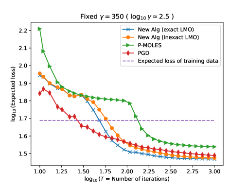
Figure 1: Expected loss as a function of the number of iterations for $\gamma=350$, compared to noiseless data.

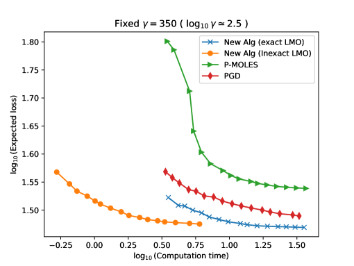
Figure 2: Computational time versus error for inexact LMO with $\gamma=350$, demonstrating the computational efficiency.

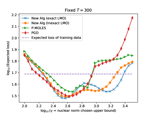
Figure 3: Performance of four algorithms at $T=300$ iterations. Performance dips for very small or large $\gamma$.

5 Conclusions and Open Problems

This paper tackles the problem of solving general convex optimization with functional constraints without projecting onto the feasible set. Previous studies on projection-free algorithms mainly focused on smooth problems and/or did not consider functional constraints. Our experiments and convergence theorems demonstrate that our algorithm performs comparably to projected stochastic subgradient descent methods, making it a viable alternative in scenarios where projection-free approaches are preferred.

An open problem is whether our algorithm can incorporate benefits from mirror descent [92, 93], an established method that substitutes the Euclidean norm in projected subgradient descent with Bregman divergence, leading to enhanced performance in specific contexts, such as when dealing with a probability simplex. Another question is whether, similar to projected subgradient descent, we can achieve an improved rate for nonsmooth, strongly convex optimization [94]. Another important area to explore is how our method works in online settings. This is especially relevant since projection-free online convex optimization is a highly discussed topic today [95, 58, 61, 57, 37, 62].

Additionally, it is worth investigating whether the subgradient can be computed on points within the feasible set $\mathcal{X}$, rather than using $y_{t}\in\mathcal{Y}$ that may lie outside of the set $\mathcal{X}$. Notably, our algorithm is not unique in utilizing subgradients outside the feasible set [59, 38, 89, 64, 63, 36, 96].

Declarations

Funding This research received partial support from the National Science Foundation (NSF), including NSF CCF 1718477 and NSF SpecEES 1824418 grants.

Code and data availability The data used in our simulation is synthetic. The codes and synthetically generated data are accessible at github.com/kamiarasgari.

Competing interests The authors declare that they have no competing interests relevant to the content of this article.

Appendix A Remaining proofs

Proof of Lemma 1.

Lipschitz continuity of $f$: Let $x,y\in\mathcal{Y}$. Consider stochastic subgradients $s_{x}$ of $f$ at $x$. This vector, as per Assumption 3.iii, satisfy the following conditions:

$$\mathbb{E}\{s_{x}\mid x\}\in\partial f(x),\quad\sqrt{\mathbb{E}\left\{\left\|s_{x}\right\|^{2}\mid x\right\}}\leq L,$$

Exploiting the convexity of $f$ and applying the Cauchy–Schwarz inequality, we arrive at:

$$f(x)-f(y)\leq\left\langle\mathbb{E}\{s_{x}\mid x\}\,,\,x-y\right\rangle\leq\left\|\mathbb{E}\{s_{x}\mid x\}\right\|\|x-y\|.$$

Using Jensen’s inequality for the norm function (which is convex) and the nonnegativity of the variance, we can further deduce:

$$\left\|\mathbb{E}\{s_{x}\mid x\}\right\|\leq\mathbb{E}\{\left\|s_{x}\right\|\mid x\}\leq\sqrt{\mathbb{E}\left\{\left\|s_{x}\right\|^{2}\mid x\right\}}\leq L$$

These implications lead to:

$$f(x)-f(y)\leq L\|x-y\|.$$

Similarly, considering a stochastic subgradient $s_{y}$ of $f$ at point $y$, we can deduce:

$$f(y)-f(x)\leq L\|x-y\|.$$

This concludes the proof of Lipschitz continuity for $f$.

Lipschitz continuity of $h_{i}$: Let $x,y\in\mathcal{Y}$. Consider stochastic subgradients $g_{x}$ of $h_{i}$ at $x$. This vector, as per Assumption 3.iii, satisfy the following conditions:

$$\mathbb{E}\{g_{x}\mid x\}\in\partial h_{i}(x),\quad\left\|g_{x}\right\|\leq G_{i},$$

Similar to the analysis of function $f$, by exploiting the convexity of $h_{i}$, applying the Cauchy–Schwarz inequality, and using Jensen’s inequality we arrive at:

$$h_{i}(x)-h_{i}(y)\leq\mathbb{E}\{\left\|g_{x}\right\|\mid x\}\|x-y\|\leq G_{i}\|x-y\|.$$

Similarly, considering a stochastic subgradient $g_{y}$ of $h_{i}$ at point $y$, we can deduce:

$$h_{i}(y)-h_{i}(x)\leq G_{i}\|x-y\|.$$

This concludes the proof of Lipschitz continuity for $h_{i}$.

Lipschitz continuity of $h$: Lipschitz continuity of $h_{i}$ implies:

$$(h_{i}(y)-h_{i}(x))^{2}\leq G_{i}^{2}\|x-y\|^{2}.$$

By summing over $i\in\{1,\ldots,m\}$ we get:

$$\left\|h(y)-h(x)\right\|^{2}_{2}\leq\sum_{i=1}^{m}G_{i}^{2}\|x-y\|^{2}\leq G^{2}\|x-y\|^{2}.$$

This concludes the proof of Lipschitz continuity for $h$. ∎

Proof of Lemma 4:.

We initiate our proof with Line 10, which states that $y_{t+1}=\operatorname{PO}_{\mathcal{Y}}\{\tilde{y}_{t+1}\}$. By applying the definition of projection from equation (2), we can express it as:

$$y_{t+1}=\arg\min_{y\in\mathcal{Y}}\{\|y-\tilde{y}_{t+1}\|\}=\arg\min_{y\in\mathcal{Y}}\{\|y-\tilde{y}_{t+1}\|^{2}\}.$$

Now, utilizing Line 9, we obtain:

$$\|y-\tilde{y}_{t+1}\|^{2}=\left\|y-\frac{\left(\alpha+2G^{2}\beta\right)y_{t}+\eta x_{t+1}-p_{t}}{\alpha+2G^{2}\beta+\eta}\right\|^{2}$$

Define $\Omega\coloneqq\alpha+2G^{2}\beta+\eta$. This allows us to further simplify it as:

$$y_{t+1}=\arg\min_{y\in\mathcal{Y}}\left\{\Omega\|y\|^{2}-2\left\langle\left(\alpha+2G^{2}\beta\right)y_{t}+\eta x_{t+1}\,,\,y\right\rangle+2\left\langle p_{t}\,,\,y\right\rangle\right\}$$

Continuing with the simplification and invoking Line 8, which defines the temporary variable $p_{t}$, we arrive at:

$$y_{t+1}= \arg\min_{y\in\mathcal{Y}}\Bigg{\{}\frac{\eta}{2}\|y-x_{t+1}\|^{2}+\frac{\alpha+2G^{2}\beta}{2}\|y-y_{t}\|^{2}$$

$$+\left\langle\eta Q_{t}\,,\,y\right\rangle+\left\langle s_{t}\,,\,y\right\rangle+\left\langle\beta\sum_{i=1}^{m}(W_{i,t}+h_{i}(y_{t}))g_{i,t}\,,\,y\right\rangle\Bigg{\}}$$

$$= \arg\min_{y\in\mathcal{Y}}\Bigg{\{}\frac{\eta}{2}\|y-x_{t+1}\|^{2}+\frac{\alpha+2G^{2}\beta}{2}\|y-y_{t}\|^{2}+\eta\left\langle Q_{t}\,,\,y-x_{t+1}\right\rangle$$

$$+\left\langle s_{t}\,,\,y-y_{t}\right\rangle+\beta\sum_{i=1}^{m}(W_{i,t}+h_{i}(y_{t}))\left(h_{i}(y_{t})+\left\langle g_{i,t}\,,\,y\right\rangle\right)\Bigg{\}}.$$

Finally, by utilizing the linearized function $l_{t}$ defined in equation (14), we conclude the proof. ∎

A.1 Proof of Theorem 2

Lemma 6.

: Line 14 implies the following inequality:

$$\|\left[h(\bar{x})\right]_{+}\|_{2}\leq\frac{\|W_{T}\|_{2}+\|\left[h(y_{T})\right]_{+}\|_{2}}{T}+\frac{G}{T}\sum_{t=1}^{T-1}\|y_{t+1}-y_{t}\|+G\|\bar{y}-\bar{x}\|.$$

Proof.

: Fix $i\in\{1,\ldots,m\}$. Line 14 of the algorithm implies:

$$W_{i,t+1}\geq W_{i,t}+h_{i}(y_{t})+\left\langle g_{i,t}\,,\,y_{t+1}-y_{t}\right\rangle$$

Using the Cauchy–Schwarz inequality we get:

$$W_{i,t+1}\geq W_{i,t}+h_{i}(y_{t})+\left\|g_{i,t}\right\|\|y_{t+1}-y_{t}\|$$

Summing over $t\in\{1,\ldots,T-1\}$ gives:

$$W_{i,T}\geq W_{i,1}+\sum_{t=1}^{T-1}h_{i}(y_{t})+\sum_{t=1}^{T-1}\left\|g_{i,t}\right\|\|y_{t+1}-y_{t}\|$$

Using the fact that $W_{i,1}\geq 0$ from Lemma 3, and adding $h_{i}(y_{T})$ to both sides, we get:

$$\sum_{t=1}^{T}h_{i}(y_{t})\leq W_{i,T}+h_{i}(y_{T})-\sum_{t=1}^{T-1}\left\|g_{i,t}\right\|\|y_{t+1}-y_{t}\|$$

Furthermore, by applying Jensen’s inequality we get:

$$h_{i}(\bar{y})\leq\frac{1}{T}\left(W_{i,T}+h_{i}(y_{T})+\sum_{t=1}^{T-1}\left\|g_{i,t}\right\|\|y_{t+1}-y_{t}\|\right)$$

Adding $h_{i}(\bar{x})-h_{i}(\bar{y})$ to both sides of the inequality we get

$$h_{i}(\bar{x})\leq\frac{1}{T}\left(W_{i,T}+h_{i}(y_{T})+\sum_{t=1}^{T-1}\left\|g_{i,t}\right\|\|y_{t+1}-y_{t}\|\right)+h_{i}(\bar{x})-h_{i}(\bar{y})$$

The positive part function $[\cdot]_{+}$ is nondecreasing. Therefore:

$$[h_{i}(\bar{x})]_{+}\leq\left[\frac{1}{T}\left(W_{i,T}+h_{i}(y_{T})+\sum_{t=1}^{T-1}\left\|g_{i,t}\right\|\|y_{t+1}-y_{t}\|\right)+h_{i}(\bar{x})-h_{i}(\bar{y})\right]_{+}$$

Lemma 3, states $W_{i,T}\geq 0$. Using the general property that for any two nonnegative real numbers $a$ and $b$, $[a+b]_{+}\leq[a]_{+}+[b]_{+}$, we obtain:

$$[h_{i}(\bar{x})]_{+}\leq\frac{W_{i,T}+\left[h_{i}(y_{T})\right]_{+}}{T}+\frac{1}{T}\sum_{t=1}^{T-1}\left\|g_{i,t}\right\|\|y_{t+1}-y_{t}\|+\left[h_{i}(\bar{x})-h_{i}(\bar{y})\right]_{+}$$ (31)

To continue the proof, consider the following inequality. Fix arbitrary vectors $a,b_{1},\ldots,b_{K}\in\mathbb{R}_{+}^{m}$. If vector $a$ is component-wise smaller than or equal to the vector $\sum_{k=1}^{K}b_{k}$, then we have $\|a\|_{2}\leq\left\|\sum_{k=1}^{K}b_{k}\right\|_{2}$. Utilizing the triangle inequality this gives: $\|a\|_{2}\leq\sum_{k=1}^{K}\left\|b_{k}\right\|_{2}$. Thus, considering the (31) as an inequality for $i$-th element of vectors belonging to $\mathbb{R}^{m}_{+}$, we can write:

$$\left\|[h(\bar{x})]_{+}\right\|_{2}\leq \frac{\left\|W_{T}\right\|_{2}+\left\|\left[h_{i}(y_{T})\right]_{+}\right\|_{2}}{T}+\frac{1}{T}\sum_{t=1}^{T-1}\sqrt{\sum_{i=1}^{m}\left\|g_{i,t}\right\|^{2}}\|y_{t+1}-y_{t}\|$$

$$+\left\|\left[h(\bar{x})-h(\bar{y})\right]_{+}\right\|_{2}$$

$$\overset{\text{(a)}}{\leq} \frac{\left\|W_{T}\right\|_{2}+\left\|\left[h_{i}(y_{T})\right]_{+}\right\|_{2}}{T}+\frac{G}{T}\sum_{t=1}^{T-1}\|y_{t+1}-y_{t}\|+\left\|\left[h(\bar{x})-h(\bar{y})\right]_{+}\right\|_{2}$$

$$\overset{\text{(b)}}{\leq} \frac{\left\|W_{T}\right\|_{2}+\left\|\left[h_{i}(y_{T})\right]_{+}\right\|_{2}}{T}+\frac{G}{T}\sum_{t=1}^{T-1}\|y_{t+1}-y_{t}\|+\left\|h(\bar{x})-h(\bar{y})\right\|_{2}$$

$$\overset{\text{(c)}}{\leq} \frac{\left\|W_{T}\right\|_{2}+\left\|\left[h_{i}(y_{T})\right]_{+}\right\|_{2}}{T}+\frac{G}{T}\sum_{t=1}^{T-1}\|y_{t+1}-y_{t}\|+G\|\bar{y}-\bar{x}\|$$

Here, (a) is by Assumption 3.iii; the simple fact that for any $a\in\mathbb{R}^{m}$, we have $\left\|[x]_{+}\right\|_{2}\leq\left\|x\right\|_{2}$ implies (b); and (c) in by Lemma 1. ∎

Proof of Theorem 2:.

The initial steps of this proof closely resemble those in the proof of Theorem 1. Just as we did in that proof, we will denote the right-hand-side and left-hand-side of (22) as $\textbf{RHS}_{t}$ and $\textbf{LHS}_{t}$, respectively. The previously derived equation (23) is demonstrated here:

$$\sum_{t=1}^{T-1}\mathbb{E}\left\{\textbf{LHS}_{t}\right\}\geq\frac{\eta}{2}\mathbb{E}\left\{\|Q_{T}\|^{2}-\|Q_{1}\|^{2}\right\}+\frac{G^{2}\beta}{2}\sum_{t=1}^{T-1}\mathbb{E}\left\{\|y_{t+1}-y_{t}\|^{2}\right\}\\ -\sum_{t=1}^{T-1}\frac{\mathbb{E}\left\{\|s_{t}\|^{2}\right\}}{2\alpha}+\frac{\beta}{2}\mathbb{E}\left\{\|W_{T}\|_{2}^{2}-\|W_{1}\|_{2}^{2}-\|\left[-h(y_{T})\right]_{+}\|_{2}^{2}+\left\|h(y_{1})\right\|_{2}^{2}\right\}$$

Lines 3 and 5 of the algorithm lead to the following implications, respectively:

$$Q_{1}=\textbf{0},$$

$$\|W_{1}\|_{2}=\|\left[-h(y_{1})\right]_{+}\|_{2}\leq\|h(y_{1})\|_{2}.$$

Utilizing the inequalities mentioned above, we obtain:

$$\begin{split}\sum_{t=1}^{T-1}\mathbb{E}\left\{\textbf{LHS}_{t}\right\}\geq&\frac{\eta}{2}\mathbb{E}\left\{\|Q_{T}\|^{2}\right\}+\frac{G^{2}\beta}{2}\sum_{t=1}^{T-1}\mathbb{E}\left\{\|y_{t+1}-y_{t}\|^{2}\right\}\\ &-\sum_{t=1}^{T-1}\frac{\mathbb{E}\left\{\|s_{t}\|^{2}\right\}}{2\alpha}+\frac{\beta}{2}\mathbb{E}\left\{\|W_{T}\|_{2}^{2}-\|\left[-h(y_{T})\right]_{+}\|_{2}^{2}\right\}\end{split}$$ (32)

Note that, unlike what we did in (24), we did not utilize the inequality $\|W_{T}\|_{2}\geq\|\left[-h(y_{T})\right]_{+}\|_{2}$ in (32).

For the $\textbf{RHS}_{t}$, we use the previously derived (25), which is demonstrated below:

$$\sum_{t=1}^{T-1}\mathbb{E}\left\{\textbf{RHS}_{t}\right\}\leq \sum_{t=1}^{T-1}\mathbb{E}\left\{\left\langle s_{t}\,,\,x^{*}-y_{t}\right\rangle\right\}-\frac{\alpha+2G^{2}\beta}{2}\mathbb{E}\left\{\|x^{*}-y_{T}\|^{2}\right\}$$

$$+\frac{\alpha+2G^{2}\beta}{2}D^{2}+T\eta\frac{D^{2}+2\delta}{2}.$$ (Eq.(25) copied)

Using (27) in the above equation we get:

$$\begin{split}\sum_{t=1}^{T-1}\mathbb{E}\left\{\textbf{RHS}_{t}\right\}\leq&\sum_{t=1}^{T}\mathbb{E}\left\{\left\langle s_{t}\,,\,x^{*}-y_{t}\right\rangle\right\}-G^{2}\beta\mathbb{E}\left\{\|x^{*}-y_{T}\|^{2}\right\}\\ &+\frac{\alpha+2G^{2}\beta}{2}D^{2}+T\eta\frac{D^{2}+2\delta}{2}+\frac{\mathbb{E}\left\{\|s_{T}\|^{2}\right\}}{2\alpha}.\end{split}$$ (33)

Consider the following derivation. Starting from equation (19), we obtain the following expression:

$$\begin{split}\sum_{t=1}^{T}\mathbb{E}\left\{\left\langle s_{t}\,,\,x^{*}-y_{t}\right\rangle\right\}\leq&\sum_{t=1}^{T}\mathbb{E}\left\{f(x^{*})-f(y_{t})\right\}\\ \text{(by Lemma~{}\ref{lem:Lagrange})}\leq&\sum_{t=1}^{T}\mathbb{E}\left\{\mu^{\top}h(y_{t})+\left\langle\lambda\,,\,x_{t}-y_{t}\right\rangle\right\}\\ \text{(by the definition of $\bar{x}$, $\bar{y}$)}=&\sum_{t=1}^{T}\mathbb{E}\left\{\mu^{\top}h(y_{t})\right\}+T\left\langle\lambda\,,\,\mathbb{E}\left\{\bar{x}-\bar{y}\right\}\right\rangle\end{split}$$ (34)

For any $i\in\{1,\ldots,m\}$, Line 14 of the algorithm implies:

$$\begin{split}h_{i}(y_{t})\leq&W_{i,t+1}-W_{i,t}-\left\langle g_{i,t}\,,\,y_{t+1}-y_{t}\right\rangle\\ \text{(by Cauchy-Schwarz)}\leq&W_{i,t+1}-W_{i,t}+\left\|g_{i,t}\right\|\left\|y_{t+1}-y_{t}\right\|\end{split}$$ (35)

Summing (35) over $t$ in the range $t\in\{1,\ldots,T-1\}$ yields:

$$\begin{split}\sum_{t=1}^{T-1}h_{i}(y_{t})\leq&\sum_{t=1}^{T-1}\left(W_{i,t+1}-W_{i,t}+\left\|g_{i,t}\right\|\left\|y_{t+1}-y_{t}\right\|\right)\\ =&W_{i,T}-W_{i,1}+\sum_{t=1}^{T-1}\left\|g_{i,t}\right\|\left\|y_{t+1}-y_{t}\right\|\\ \text{($W_{i,1}\geq 0$ by Lemma~{}\ref{lem:results from Alg})}\leq&W_{i,T}+\sum_{t=1}^{T-1}\left\|g_{i,t}\right\|\left\|y_{t+1}-y_{t}\right\|\end{split}$$ (36)

Multiplying both sides of (36) by $\mu_{i}\geq 0$ and summing over $i$ yields:

$$\sum_{i=1}^{m}\mu_{i}\sum_{t=1}^{T-1}h_{i}(y_{t})\leq \mu^{\top}W_{T}+\sum_{i=1}^{m}\mu_{i}\sum_{t=1}^{T-1}\left\|g_{i,t}\right\|\left\|y_{t+1}-y_{t}\right\|$$

$$= \mu^{\top}W_{T}+\sum_{t=1}^{T-1}\left(\sum_{i=1}^{m}\mu_{i}\left\|g_{i,t}\right\|\right)\left\|y_{t+1}-y_{t}\right\|$$

$$\text{(by Cauchy-Schwarz)}\leq \mu^{\top}W_{T}+\sum_{t=1}^{T-1}\left(\left\|\mu\right\|_{2}\sqrt{\sum_{i=1}^{m}\left\|g_{i,t}\right\|^{2}}\right)\left\|y_{t+1}-y_{t}\right\|$$

$$\text{(by Assumption~{}\ref{assum:SFO})}\leq \mu^{\top}W_{T}+\|\mu\|_{2}G\sum_{t=1}^{T-1}\|y_{t+1}-y_{t}\|$$

Replacing this inequality in (34) results in:

$$\begin{split}\sum_{t=1}^{T}\mathbb{E}\left\{\left\langle s_{t}\,,\,x^{*}-y_{t}\right\rangle\right\}\leq&\mathbb{E}\left\{\mu^{\top}h(y_{T})+\mu^{\top}W_{T}\right\}\\ &+G\|\mu\|_{2}\sum_{t=1}^{T-1}\mathbb{E}\left\{\|y_{t+1}-y_{t}\|\right\}+T\left\langle\lambda\,,\,\mathbb{E}\left\{\bar{x}-\bar{y}\right\}\right\rangle\end{split}$$ (37)

Substituting equations (32), (33), and (37) into (22) and rearranging the terms, we obtain:

$$\begin{split}&\frac{\eta}{2}\mathbb{E}\left\{\|Q_{T}\|^{2}\right\}-T\left\langle\lambda\,,\,\mathbb{E}\left\{\bar{x}-\bar{y}\right\}\right\rangle\\ &+\frac{G^{2}\beta}{2}\sum_{t=1}^{T-1}\mathbb{E}\left\{\|y_{t+1}-y_{t}\|^{2}\right\}-G\|\mu\|_{2}\sum_{t=1}^{T-1}\mathbb{E}\left\{\|y_{t+1}-y_{t}\|\right\}\\ &+\frac{\beta}{2}\mathbb{E}\left\{\|W_{T}\|_{2}^{2}-\|\left[-h(y_{T})\right]_{+}\|_{2}^{2}\right\}-\mathbb{E}\left\{\mu^{\top}h(y_{T})+\mu^{\top}W_{T}\right\}\\ \leq&\sum_{t=1}^{T}\frac{\mathbb{E}\left\{\|s_{t}\|^{2}\right\}}{2\alpha}-G^{2}\beta\mathbb{E}\left\{\|x^{*}-y_{T}\|^{2}\right\}\\ &+\frac{\alpha+2G^{2}\beta}{2}D^{2}+T\eta\frac{D^{2}+2\delta}{2}\end{split}$$ (38)

Consider the two terms in the above equation: $\frac{\beta}{2}\mathbb{E}\left\{-\|\left[-h(y_{T})\right]_{+}\|_{2}^{2}\right\}$ from the left-hand-side and $-G^{2}\beta\mathbb{E}\left\{\|x^{*}-y_{T}\|^{2}\right\}$ from the right-hand-side. To simplify both of these terms, we use the Lipschitz continuity of $h$ (see Lemma 1):

$$\left\|h(y_{T})-h(x^{*})\right\|_{2}\leq G\left\|x^{*}-y_{T}\right\|$$

By using reverse triangle inequality we get

$$\left\|h(y_{T})\right\|_{2}\leq\left\|h(x^{*})\right\|_{2}+G\left\|x^{*}-y_{T}\right\|$$

Using the simple fact that $(a+b)^{2}\leq 2a^{2}+2b^{2}$ we get:

$$\left\|h(y_{T})\right\|_{2}^{2}\leq 2\left\|h(x^{*})\right\|_{2}^{2}+2G^{2}\left\|x^{*}-y_{T}\right\|^{2}$$

To connect this result to $\|\left[-h(y_{T})\right]_{+}\|_{2}$, note that for any arbitrary vector $v\in\mathbb{R}^{m}$, the inequality $\|v\|_{2}^{2}=\|\left[-v\right]_{+}\|_{2}^{2}+\|\left[v\right]_{+}\|_{2}^{2}$ holds. Therefore, for $h(y_{T})\in\mathbb{R}^{m}$, we can write:

$$\|\left[-h(y_{T})\right]_{+}\|_{2}^{2}\leq 2\|h(x^{*})\|^{2}+2G^{2}\|x^{*}-y_{T}\|^{2}-\|\left[h(y_{T})\right]_{+}\|_{2}^{2}$$ (39)

Utilizing equation (39) within (38) and further simplifying by applying $Q_{T}=T(\bar{y}-\bar{x})$, and the inequality $\mathbb{E}\{\|s_{t}\|^{2}\}\leq L^{2}$, we obtain:

$$(\textbf{LHS}_{a}\coloneqq) \frac{T^{2}\eta}{2}\mathbb{E}\left\{\|\bar{y}-\bar{x}\|^{2}\right\}-T\left\langle\lambda\,,\,\mathbb{E}\left\{\bar{x}-\bar{y}\right\}\right\rangle$$

$$(\textbf{LHS}_{b}\coloneqq) +\frac{G^{2}\beta}{2}\sum_{t=1}^{T-1}\mathbb{E}\left\{\|y_{t+1}-y_{t}\|^{2}\right\}-G\|\mu\|_{2}\sum_{t=1}^{T-1}\mathbb{E}\left\{\|y_{t+1}-y_{t}\|\right\}$$

$$(\textbf{LHS}_{c}\coloneqq) +\frac{\beta}{2}\mathbb{E}\left\{\|W_{T}\|_{2}^{2}+\|\left[h(y_{T})\right]_{+}\|_{2}^{2}\right\}-\mathbb{E}\left\{\mu^{\top}h(y_{T})+\mu^{\top}W_{T}\right\}$$

$$\leq \beta\|h(x^{*})\|_{2}^{2}+\frac{TL^{2}}{2\alpha}+\frac{\alpha+2G^{2}\beta}{2}D^{2}+T\eta\frac{D^{2}+2\delta}{2}$$ (40)

Here, the left-hand-side is divided into three terms, each of which is simplified as follows:

$$\textbf{LHS}_{a}= \frac{T^{2}\eta}{2}\mathbb{E}\left\{\|\bar{y}-\bar{x}\|^{2}\right\}-T\left\langle\lambda\,,\,\mathbb{E}\left\{\bar{x}-\bar{y}\right\}\right\rangle$$

$$\overset{\text{(a)}}{\geq} \frac{T^{2}\eta}{2}\left(\mathbb{E}\left\{\|\bar{y}-\bar{x}\|\right\}\right)^{2}-T\|\lambda\|\mathbb{E}\left\{\|\bar{y}-\bar{x}\|\right\}$$

$$\overset{\text{(b)}}{=} \frac{1}{2}\left(T\sqrt{\eta}\mathbb{E}\left\{\|\bar{y}-\bar{x}\|\right\}-\frac{1}{\sqrt{\eta}}\|\lambda\|\right)^{2}-\frac{\|\lambda\|^{2}}{2\eta}$$

where (a) follows from the Cauchy–Schwarz and Jensen’s inequalities, and (b) is obtained by completing the square.

$$\textbf{LHS}_{b}= \frac{G^{2}\beta}{2}\sum_{t=1}^{T-1}\mathbb{E}\left\{\|y_{t+1}-y_{t}\|^{2}\right\}-G\|\mu\|_{2}\sum_{t=1}^{T-1}\mathbb{E}\left\{\|y_{t+1}-y_{t}\|\right\}$$

$$\overset{\text{(a)}}{\geq} \frac{G^{2}\beta}{2}(T-1)\left(\frac{1}{T-1}\sum_{t=1}^{T-1}\mathbb{E}\left\{\|y_{t+1}-y_{t}\|\right\}\right)^{2}$$

$$-G\|\mu\|_{2}\sum_{t=1}^{T-1}\mathbb{E}\left\{\|y_{t+1}-y_{t}\|\right\}$$

$$\overset{\text{(b)}}{=} \frac{1}{2}\left(\sqrt{\frac{G^{2}\beta}{T-1}}\sum_{t=1}^{T-1}\mathbb{E}\left\{\|y_{t+1}-y_{t}\|\right\}-\sqrt{\frac{T-1}{\beta}}\|\mu\|_{2}\right)^{2}-{\frac{T-1}{2\beta}}\|\mu\|_{2}^{2}$$

here, (a) is justified by Jensen’s inequality, and (b) is obtained by completing the square.

$$\textbf{LHS}_{c}= \frac{\beta}{2}\mathbb{E}\left\{\|W_{T}\|_{2}^{2}+\|\left[h(y_{T})\right]_{+}\|_{2}^{2}\right\}-\mathbb{E}\left\{\mu^{\top}h(y_{T})+\mu^{\top}W_{T}\right\}$$

$$\overset{\text{(a)}}{\geq} \frac{\beta}{4}\left(\mathbb{E}\left\{\|W_{T}\|_{2}+\|\left[h(y_{T})\right]_{+}\|_{2}\right\}\right)^{2}-\mathbb{E}\left\{\mu^{\top}h(y_{T})+\mu^{\top}W_{T}\right\}$$

$$\overset{\text{(b)}}{\geq} \frac{\beta}{4}\left(\mathbb{E}\left\{\|W_{T}\|_{2}+\|\left[h(y_{T})\right]_{+}\|_{2}\right\}\right)^{2}-\|\mu\|_{2}\mathbb{E}\left\{\|\left[h(y_{T})\right]_{+}\|_{2}+\|W_{T}\|_{2}\right\}$$

$$\overset{\text{(c)}}{=} \left(\frac{\sqrt{\beta}}{2}\mathbb{E}\left\{\|W_{T}\|_{2}+\|\left[h(y_{T})\right]_{+}\|_{2}\right\}-\frac{\|\mu\|_{2}}{\sqrt{\beta}}\right)^{2}-\frac{\|\mu\|^{2}_{2}}{\beta}$$

where (a) holds by Jensen’s inequality; (b) holds because of the the Cauchy–Schwarz inequality and the fact that $\mu^{\top}h(y_{T})\leq\mu^{\top}[h(y_{T})]_{+}$; and (c) is by completing the square.

By employing these three inequalities, the equation (40) can be rendered in a simplified form as follows:

$$\frac{1}{2}\left(T\sqrt{\eta}\mathbb{E}\left\{\|\bar{y}-\bar{x}\|\right\}-\frac{1}{\sqrt{\eta}}\|\lambda\|\right)^{2}$$

$$\frac{1}{2}\left(\sqrt{\frac{G^{2}\beta}{T-1}}\sum_{t=1}^{T-1}\mathbb{E}\left\{\|y_{t+1}-y_{t}\|\right\}-\sqrt{\frac{T-1}{\beta}}\|\mu\|_{2}\right)^{2}$$

$$+\left(\frac{\sqrt{\beta}}{2}\mathbb{E}\left\{\|W_{T}\|_{2}+\|\left[h(y_{T})\right]_{+}\|_{2}\right\}-\frac{\|\mu\|_{2}}{\sqrt{\beta}}\right)^{2}$$

$$\leq \underbrace{\beta\|h(x^{*})\|_{2}^{2}+G^{2}D^{2}\beta+{\frac{T+1}{2\beta}}\|\mu\|_{2}^{2}+\frac{TL^{2}}{2\alpha}+\frac{\alpha D^{2}}{2}+T\eta\frac{D^{2}+2\delta}{2}+\frac{\|\lambda\|^{2}}{2\eta}}_{\Gamma}$$ (41)

The equation above can be employed to individually bound each of the three left-hand-side terms with respect to the newly defined parameter $\Gamma$. This implies:

$$\frac{1}{2}\left(T\sqrt{\eta}\mathbb{E}\left\{\|\bar{y}-\bar{x}\|\right\}-\frac{1}{\sqrt{\eta}}\|\lambda\|\right)^{2}\leq \Gamma$$

$$\frac{1}{2}\left(\sqrt{\frac{G^{2}\beta}{T-1}}\sum_{t=1}^{T-1}\mathbb{E}\left\{\|y_{t+1}-y_{t}\|\right\}-\sqrt{\frac{T-1}{\beta}}\|\mu\|_{2}\right)^{2}\leq \Gamma$$

$$\left(\frac{\sqrt{\beta}}{2}\mathbb{E}\left\{\|W_{T}\|_{2}+\|\left[h(y_{T})\right]_{+}\|_{2}\right\}-\frac{\|\mu\|_{2}}{\sqrt{\beta}}\right)^{2}\leq \Gamma$$

Which become

$$\begin{split}\mathbb{E}\left\{\|\bar{y}-\bar{x}\|\right\}\leq&\sqrt{\frac{2}{T^{2}\eta}\Gamma}+\frac{\|\lambda\|}{T\eta}\\ \sum_{t=1}^{T-1}\mathbb{E}\left\{\|y_{t+1}-y_{t}\|\right\}\leq&\sqrt{\frac{2T}{G^{2}\beta}\Gamma}+\frac{T\|\mu\|_{2}}{G\beta}\\ \mathbb{E}\left\{\|W_{T}\|_{2}+\|\left[h(y_{T})\right]_{+}\|_{2}\right\}\leq&\sqrt{\frac{4}{\beta}\Gamma}+\frac{2\|\mu\|_{2}}{\beta}\end{split}$$ (42)

Substituting (42) in Lemma 6 yields:

$$\begin{split}\mathbb{E}\left\{\|\left[h(\bar{x})\right]_{+}\|_{2}\right\}\leq&\frac{G}{T}\left(\sqrt{\frac{2T}{G^{2}\beta}\Gamma}+\frac{T\|\mu\|_{2}}{{G\beta}}\right)\\ &+\frac{1}{T}\left(\sqrt{\frac{4}{\beta}\Gamma}+\frac{2\|\mu\|_{2}}{\beta}\right)\\ &+G\left(\sqrt{\frac{2}{T^{2}\eta}\Gamma}+\frac{\|\lambda\|}{T\eta}\right)\\ =&\sqrt{\frac{\Gamma}{T}}\left(\sqrt{\frac{2}{\beta}}+\sqrt{\frac{4}{T\beta}}+\sqrt{\frac{2G^{2}}{T\eta}}\right)\\ &+\frac{\|\mu\|_{2}}{\beta}+\frac{2\|\mu\|_{2}}{T\beta}+\frac{G\|\lambda\|}{T\eta},\end{split}$$ (43)

Parameter Selection 1 (ParSel.1): By substituting $\eta=\epsilon,\alpha=\beta=1/\epsilon,$ and $T\geq 1/\epsilon^{2}$ into (43) and utilizing the $\Gamma$ defined in (41), we obtain:

$$\frac{\Gamma}{T}\leq\mathcal{O}\left(\epsilon\right),$$

and thus

$$\mathbb{E}\left\{\|\left[h(\bar{x})\right]_{+}\|_{2}\right\}\leq\mathcal{O}\left(\epsilon\right).$$

Parameter Selection 2 (ParSel.2): To proceed, we must first simplify (43) further.

$$\begin{split}\mathbb{E}\left\{\|\left[h(\bar{x})\right]_{+}\|_{2}\right\}\overset{\text{(a)}}{\leq}&\sqrt{\frac{\Gamma}{T}}\left(\left(1+\sqrt{2}\right)\sqrt{\frac{2}{\beta}}+\sqrt{\frac{2G^{2}}{T\eta}}\right)+\frac{3\|\mu\|_{2}}{\beta}+\frac{G\|\lambda\|}{T\eta}\\ =&\sqrt{\frac{\Gamma}{T}\left(1+\sqrt{2}\right)^{2}\frac{2}{\beta}}+\sqrt{\frac{\Gamma}{T}\frac{2G^{2}}{T\eta}}+\sqrt{\frac{9\|\mu\|_{2}^{2}}{\beta^{2}}}+\sqrt{\frac{G^{2}\|\lambda\|^{2}}{T^{2}\eta^{2}}}\\ \overset{\text{(b)}}{\leq}&\sqrt{\frac{\Gamma}{T}\left(\frac{47}{\beta}+\frac{8G^{2}}{T\eta}\right)+\frac{36\|\mu\|_{2}^{2}}{\beta^{2}}+\frac{4G^{2}\|\lambda\|^{2}}{T^{2}\eta^{2}}}\\ \overset{\text{(c)}}{\leq}&\sqrt{\frac{\Gamma}{T}\left(\frac{47}{\beta}+\frac{8G^{2}}{T\eta}\right)+\frac{36\|\mu\|_{2}^{2}}{\beta^{2}}+\frac{4G^{2}\left(L+\left\|\mu\right\|_{2}G\right)^{2}}{T^{2}\eta^{2}}}\end{split}$$ (44)

here, for (a), we exploit the fact that $T\geq 1$; for (b), we apply Jensen’s inequality to the concave square root function; and finally, (c) follows from (5).

Simplifying the term $\sqrt{\frac{\Gamma}{T}}$ using the definition from (41) results in:

$$\begin{split}\frac{\Gamma}{T}=&\frac{\beta\|h(x^{*})\|_{2}^{2}}{T}+\frac{G^{2}D^{2}\beta}{T}+{\frac{T+1}{2\beta T}}\|\mu\|_{2}^{2}+\frac{L^{2}}{2\alpha}+\frac{\alpha D^{2}}{2T}+\eta\frac{D^{2}+2\delta}{2}+\frac{\|\lambda\|^{2}}{2T\eta}\\ \overset{\text{(a)}}{\leq}&\frac{\beta\|h(x^{*})\|_{2}^{2}}{T}+\frac{G^{2}D^{2}\beta}{T}+{\frac{\|\mu\|_{2}^{2}}{\beta}}+\frac{L^{2}}{2\alpha}+\frac{\alpha D^{2}}{2T}+\eta\frac{D^{2}+2\delta}{2}+\frac{\|\lambda\|^{2}}{2T\eta}\\ \overset{\text{(b)}}{\leq}&\frac{\beta\|h(x^{*})\|_{2}^{2}}{T}+\frac{G^{2}D^{2}\beta}{T}+{\frac{\|\mu\|_{2}^{2}}{\beta}}+\frac{L^{2}}{2\alpha}+\frac{\alpha D^{2}}{2T}+\eta\frac{D^{2}+2\delta}{2}+\frac{\left(L+\left\|\mu\right\|_{2}G\right)^{2}}{2T\eta}\end{split}$$ (45)

where (a) uses the fact that $T\geq 1$, and (b) is satisfied based on the inequality (5). Replacing $\alpha=\frac{L\sqrt{T}}{D}$, $\eta=\frac{L}{\sqrt{T\left(D^{2}+2\delta\right)}}$, and $\beta=\frac{\sqrt{T}}{GD}$ in (45) and (44) we get:

$$\frac{\Gamma}{T}\leq \frac{1}{\sqrt{T}}\left(LD+L\sqrt{D^{2}+2\delta}+GD+\frac{\|h(x^{*})\|_{2}^{2}}{GD}\right.$$

$$+\left.\left\|\mu\right\|_{2}G\sqrt{D^{2}+2\delta}+\left\|\mu\right\|_{2}^{2}\left(GD+\frac{G^{2}}{2L}\sqrt{D^{2}+2\delta}\right)\right).$$

and thus

$$\mathbb{E}\left\{\|\left[h(\bar{x})\right]_{+}\|_{2}\right\}\leq\frac{1}{\sqrt{T}}\sqrt{A_{0}+A_{1}\left\|\mu\right\|_{2}+A_{2}\|\mu\|_{2}^{2}}$$

where $A_{0}$, $A_{1}$ and $A_{2}$ are defined as follows:

$$A_{0}\coloneqq 47GLD^{2}+47GLD\sqrt{D^{2}+2\delta}+47G^{2}D^{2}+12G^{2}(D^{2}+2\delta)\\ +8G^{2}D\sqrt{D^{2}+2\delta}+8\frac{G^{3}}{L}D\sqrt{D^{2}+2\delta}+\left\|h(x^{*})\right\|_{2}^{2}\left(47+8\frac{G}{L}\frac{\sqrt{D^{2}+2\delta}}{D}\right)$$

$$A_{1}\coloneqq 16\frac{G^{3}}{L}(D^{2}+2\delta)+47G^{2}D\sqrt{D^{2}+2\delta}$$

$$A_{2}\coloneqq 55\frac{G^{3}}{L}D\sqrt{D^{2}+2\delta}+83G^{2}D^{2}+8\frac{G^{4}}{L^{2}}(D^{2}+2\delta)$$

∎

Remark 2.

If the functional constraints satisfy the assumption that for all $i\in\{1,\ldots,m\}$ there exists a point $z_{i}\in\mathcal{X}$ such that $h_{i}(z_{i})\geq 0$ (meaning that none of the functional inequalities are satisfied everywhere on the set $\mathcal{X}$), then we can write:

$$\|h(x^{*})\|_{2}\leq GD.$$

Proof.

Using Lemma 1 we have:

$$h_{i}(z)-h_{i}(x^{*})\leq G_{i}\|z_{i}-x^{*}\|.$$

Assumption 1 implies $\|z_{i}-x^{*}\|\leq D$, thus

$$h_{i}(z)-h_{i}(x^{*})\leq G_{i}D.$$

Using the fact that $h_{i}(x^{*})\leq 0$ and $h_{i}(z_{i})\geq 0$, we get

$$(h(x^{*}))^{2}\leq G_{i}^{2}D^{2}.$$

Finally, summing over $i=\{1,\ldots,m\}$ gives

$$\left\|h(x^{*})\right\|^{2}\leq\sum_{i=1}^{m}G_{i}^{2}D^{2}\leq G^{2}D^{2}$$

where we used Assumption 3.iii in the last step. ∎

References

• \bibcommenthead
• Boyd and Vandenberghe [2004] Boyd, S., Vandenberghe, L.: Convex Optimization. Cambridge University Press, Cambridge (2004). https://doi.org/10.1017/CBO9780511804441
• Palomar and Eldar [2009] Palomar, D.P., Eldar, Y.C.: Convex Optimization in Signal Processing and Communications. Cambridge University Press, Cambridge (2009). https://doi.org/10.1017/CBO9780511804458
• Sra et al. [2012] Sra, S., Nowozin, S., Wright, S.J.: Optimization for Machine Learning. The MIT Press, Cambridge (2012)
• Nesterov and Nemirovskii [1994] Nesterov, Y., Nemirovskii, A.: Interior-Point Polynomial Algorithms in Convex Programming. Society for Industrial and Applied Mathematics (SIAM), Philadelphia (1994). https://doi.org/10.1137/1.9781611970791
• Nesterov [2018] Nesterov, Y.: Lectures on Convex Optimization, 2nd ed. 2018. edn. Springer Optimization and Its Applications, 137. Springer, Cham (2018). https://doi.org/10.1007/978-3-319-91578-4
• Beck [2017] Beck, A.: First-order Methods in Optimization. Society for Industrial and Applied Mathematics (SIAM), Philadelphia (2017). https://doi.org/10.1137/1.9781611974997
• Lan [2020] Lan, G.: First-order and Stochastic Optimization Methods for Machine Learning vol. 1. Springer, Cham (2020). https://doi.org/10.1007/978-3-030-39568-1
• Perez et al. [2022] Perez, G., Ament, S., Gomes, C., Barlaud, M.: Efficient projection algorithms onto the weighted $l1$ ball. Artificial Intelligence 306, 103683 (2022)
• Combettes and Pokutta [2021] Combettes, C.W., Pokutta, S.: Complexity of linear minimization and projection on some sets. Operations Research Letters 49(4), 565–571 (2021) https://doi.org/10.1016/j.orl.2021.06.005
• Combettes [2021] Combettes, C.W.: Frank-Wolfe methods for optimization and machine learning. PhD thesis, Georgia Institute of Technology (2021)
• Juditsky and Nemirovski [2016] Juditsky, A., Nemirovski, A.: Solving variational inequalities with monotone operators on domains given by linear minimization oracles. Mathematical Programming 156(1-2), 221–256 (2016)
• Jaggi [2013] Jaggi, M.: Revisiting Frank-Wolfe: Projection-free sparse convex optimization. In: Dasgupta, S., McAllester, D. (eds.) Proceedings of the 30th International Conference on Machine Learning. Proceedings of Machine Learning Research, vol. 28, pp. 427–435. PMLR, Atlanta, Georgia, USA (2013)
• Frank and Wolfe [1956] Frank, M., Wolfe, P.: An algorithm for quadratic programming. Naval Research Logistics Quarterly 3(1-2), 95–110 (1956) https://doi.org/10.1002/nav.3800030109 https://onlinelibrary.wiley.com/doi/pdf/10.1002/nav.3800030109
• Argyriou et al. [2014] Argyriou, A., Signoretto, M., Suykens, J.: Hybrid Conditional Gradient - Smoothing Algorithms with Applications to Sparse and Low Rank Regularization (2014)
• Levitin and Polyak [1966] Levitin, E.S., Polyak, B.T.: Constrained minimization methods. USSR Computational Mathematics and Mathematical Physics 6(5), 1–50 (1966) https://doi.org/10.1016/0041-5553(66)90114-5
• Yurtsever et al. [2018] Yurtsever, A., Fercoq, O., Locatello, F., Cevher, V.: A Conditional Gradient Framework for Composite Convex Minimization with Applications to Semidefinite Programming (2018)
• Lan [2014] Lan, G.: The Complexity of Large-scale Convex Programming under a Linear Optimization Oracle (2014)
• Nemirovskij and Yudin [1983] Nemirovskij, A.S., Yudin, D.B.: Problem complexity and method efficiency in optimization (1983)
• Bubeck et al. [2015] Bubeck, S., et al.: Convex optimization: Algorithms and complexity. Foundations and Trends® in Machine Learning 8(3-4), 231–357 (2015)
• Nemirovski [1995] Nemirovski, A.: Information-based complexity of convex programming. Lecture notes 834 (1995)
• Lacoste-Julien et al. [2013] Lacoste-Julien, S., Jaggi, M., Schmidt, M., Pletscher, P.: Block-coordinate Frank-Wolfe optimization for structural SVMs. In: Dasgupta, S., McAllester, D. (eds.) Proceedings of the 30th International Conference on Machine Learning. Proceedings of Machine Learning Research, vol. 28, pp. 53–61. PMLR, Atlanta, Georgia, USA (2013)
• Jing et al. [2023] Jing, N., Fang, E.X., Tang, C.Y.: Robust matrix estimations meet frank–wolfe algorithm. Machine Learning, 1–38 (2023)
• Mu et al. [2016] Mu, C., Zhang, Y., Wright, J., Goldfarb, D.: Scalable robust matrix recovery: Frank–wolfe meets proximal methods. SIAM Journal on Scientific Computing 38(5), 3291–3317 (2016)
• Combettes and Pokutta [2023] Combettes, C.W., Pokutta, S.: Revisiting the approximate carathéodory problem via the frank-wolfe algorithm. Mathematical Programming 197(1), 191–214 (2023)
• Hazan et al. [2019] Hazan, E., Kakade, S.M., Singh, K., Soest, A.V.: Provably Efficient Maximum Entropy Exploration (2019)
• Lin et al. [2021] Lin, J.-L., Hung, W., Yang, S.-H., Hsieh, P.-C., Liu, X.: Escaping from Zero Gradient: Revisiting Action-Constrained Reinforcement Learning via Frank-Wolfe Policy Optimization (2021)
• Garber [2016] Garber, D.: Faster Projection-free Convex Optimization over the Spectrahedron (2016)
• Nesterov [2018] Nesterov, Y.: Complexity bounds for primal-dual methods minimizing the model of objective function. Mathematical Programming 171(1), 311–330 (2018) https://doi.org/10.1007/s10107-017-1188-6
• White [1993] White, D.J.: Extension of the frank-wolfe algorithm to concave nondifferentiable objective functions. Journal of Optimization Theory and Applications 78(2), 283–301 (1993) https://doi.org/10.1007/BF00939671
• Ravi et al. [2017] Ravi, S.N., Collins, M.D., Singh, V.: A Deterministic Nonsmooth Frank Wolfe Algorithm with Coreset Guarantees (2017)
• Cheung and Li [2018] Cheung, E., Li, Y.: Solving separable nonsmooth problems using frank-wolfe with uniform affine approximations. In: IJCAI, pp. 2035–2041 (2018)
• Moreau [1965] Moreau, J.J.: Proximité et dualité dans un espace hilbertien. Bulletin de la Société Mathématique de France 93, 273–299 (1965) https://doi.org/10.24033/bsmf.1625
• Nesterov [2005] Nesterov, Y.: Smooth minimization of non-smooth functions. Mathematical Programming 103(1), 127–152 (2005) https://doi.org/10.1007/s10107-004-0552-5
• Parikh and Boyd [2014] Parikh, N., Boyd, S.: Proximal algorithms. Foundations and Trends® in Optimization 1(3), 127–239 (2014) https://doi.org/10.1561/2400000003
• Yurtsever et al. [2015] Yurtsever, A., Tran Dinh, Q., Cevher, V.: A universal primal-dual convex optimization framework. Advances in Neural Information Processing Systems 28 (2015)
• Duchi et al. [2012] Duchi, J.C., Bartlett, P.L., Wainwright, M.J.: Randomized smoothing for stochastic optimization. SIAM Journal on Optimization 22(2), 674–701 (2012) https://doi.org/10.1137/110831659
• Hazan and Kale [2012] Hazan, E., Kale, S.: Projection-free online learning. In: Proceedings of the 29th International Coference on International Conference on Machine Learning. ICML’12, pp. 1843–1850. Omnipress, Madison, WI, USA (2012)
• Thekumparampil et al. [2020] Thekumparampil, K.K., Jain, P., Netrapalli, P., Oh, S.: Projection efficient subgradient method and optimal nonsmooth frank-wolfe method. Advances in Neural Information Processing Systems 33, 12211–12224 (2020)
• Polyak and Tret’yakov [1973] Polyak, V., Tret’yakov, N.: The method of penalty estimates for conditional extremum problems. USSR Computational Mathematics and Mathematical Physics 13(1), 42–58 (1973)
• Lemaréchal et al. [1995] Lemaréchal, C., Nemirovskii, A., Nesterov, Y.: New variants of bundle methods. Mathematical programming 69, 111–147 (1995)
• Lin et al. [2018] Lin, Q., Ma, R., Yang, T.: Level-set methods for finite-sum constrained convex optimization. In: International Conference on Machine Learning, pp. 3112–3121 (2018). PMLR
• Bertsekas [1999] Bertsekas, D.P.: Nonlinear Programming, 2nd edn. Athena Scientific, Raleigh (1999)
• Xu [2021] Xu, Y.: Iteration complexity of inexact augmented lagrangian methods for constrained convex programming. Mathematical Programming 185, 199–244 (2021)
• Neely and Yu [2019] Neely, M.J., Yu, H.: Lagrangian methods for o (1/t) convergence in constrained convex programs. Convex Optimization: Theory, Methods, and Applications, edited by Arto Ruud, Nova Publishers (2019)
• Lan and Monteiro [2016] Lan, G., Monteiro, R.D.: Iteration-complexity of first-order augmented lagrangian methods for convex programming. Mathematical Programming 155(1-2), 511–547 (2016)
• Wei et al. [2018] Wei, X., Yu, H., Ling, Q., Neely, M.J.: Solving Non-smooth Constrained Programs with Lower Complexity than $\mathcal{O}(1/\varepsilon)$: A Primal-Dual Homotopy Smoothing Approach (2018)
• Yu and Neely [2016] Yu, H., Neely, M.J.: A primal-dual type algorithm with the o(1/t) convergence rate for large scale constrained convex programs. In: 2016 IEEE 55th Conference on Decision and Control (CDC), pp. 1900–1905 (2016). https://doi.org/10.1109/CDC.2016.7798542
• Yu et al. [2017] Yu, H., Neely, M., Wei, X.: Online convex optimization with stochastic constraints. Advances in Neural Information Processing Systems 30 (2017)
• Neely and Yu [2017] Neely, M.J., Yu, H.: Online convex optimization with time-varying constraints. arXiv preprint arXiv:1702.04783 (2017)
• Wei and Neely [2018] Wei, X., Neely, M.J.: Primal-Dual Frank-Wolfe for Constrained Stochastic Programs with Convex and Non-convex Objectives (2018)
• Lan et al. [2021] Lan, G., Romeijn, E., Zhou, Z.: Conditional gradient methods for convex optimization with general affine and nonlinear constraints. SIAM Journal on Optimization 31(3), 2307–2339 (2021)
• Cheng et al. [2022] Cheng, Y., Lan, G., Romeijn, H.E.: Functional constrained optimization for risk aversion and sparsity control. arXiv preprint arXiv:2210.05108 (2022)
• Lee et al. [2023] Lee, D., Ho-Nguyen, N., Lee, D.: Projection-Free Online Convex Optimization with Stochastic Constraints (2023)
• Mahdavi et al. [2012] Mahdavi, M., Yang, T., Jin, R., Zhu, S., Yi, J.: Stochastic gradient descent with only one projection. Advances in neural information processing systems 25 (2012)
• Levy and Krause [2019] Levy, K., Krause, A.: Projection free online learning over smooth sets. In: The 22nd International Conference on Artificial Intelligence and Statistics, pp. 1458–1466 (2019). PMLR
• Lee et al. [2018] Lee, Y.T., Sidford, A., Vempala, S.S.: Efficient convex optimization with membership oracles. In: Conference On Learning Theory, pp. 1292–1294 (2018). PMLR
• Mhammedi [2022] Mhammedi, Z.: Efficient projection-free online convex optimization with membership oracle. In: Conference on Learning Theory, pp. 5314–5390 (2022). PMLR
• Garber and Kretzu [2022] Garber, D., Kretzu, B.: New projection-free algorithms for online convex optimization with adaptive regret guarantees. In: Conference on Learning Theory, pp. 2326–2359 (2022). PMLR
• Lu et al. [2023] Lu, Z., Brukhim, N., Gradu, P., Hazan, E.: Projection-free adaptive regret with membership oracles. In: International Conference on Algorithmic Learning Theory, pp. 1055–1073 (2023). PMLR
• Garber and Kretzu [2023] Garber, D., Kretzu, B.: New Projection-free Algorithms for Online Convex Optimization with Adaptive Regret Guarantees (2023)
• Gatmiry and Mhammedi [2023] Gatmiry, K., Mhammedi, Z.: Projection-Free Online Convex Optimization via Efficient Newton Iterations (2023)
• Garber and Kretzu [2023] Garber, D., Kretzu, B.: Projection-free online exp-concave optimization. arXiv preprint arXiv:2302.04859 (2023)
• Grimmer [2022] Grimmer, B.: Radial Duality Part II: Applications and Algorithms (2022)
• Grimmer [2023] Grimmer, B.: Radial Duality Part I: Foundations (2023)
• Bertsekas [2009] Bertsekas, D.: Convex Optimization Theory vol. 1. Athena Scientific, Raleigh (2009)
• Bertsekas [2015] Bertsekas, D.: Convex Optimization Algorithms. Athena Scientific, Raleigh (2015)
• Yu and Neely [2017] Yu, H., Neely, M.J.: A primal-dual parallel method with $\mathcal{O}(1/\epsilon)$ convergence for constrained composite convex programs. arXiv preprint arXiv:1708.00322 (2017)
• Kelly et al. [1998] Kelly, F.P., Maulloo, A.K., Tan, D.K.H.: Rate control for communication networks: shadow prices, proportional fairness and stability. Journal of the Operational Research society 49(3), 237–252 (1998)
• Bertsekas [1991] Bertsekas, D.P.: Linear Network Optimization: Algorithms and Codes. MIT press, Cambridge (1991)
• Bertsekas [1998] Bertsekas, D.P.: Network Optimization Continuous and Discrete Models. Athena Scientific, Raleigh (1998)
• Neely [2010] Neely, M.J.: Stochastic network optimization with application to communication and queueing systems. Synthesis Lectures on Communication Networks 3(1), 1–211 (2010)
• Hazan [2008] Hazan, E.: Sparse approximate solutions to semidefinite programs. In: Latin American Symposium on Theoretical Informatics, pp. 306–316 (2008). Springer
• Shinde et al. [2023] Shinde, N., Narayanan, V., Saunderson, J.: An inexact frank-wolfe algorithm for composite convex optimization involving a self-concordant function. arXiv preprint arXiv:2310.14482 (2023)
• Hampel et al. [2005] Hampel, F.R., Ronchetti, E.M., Rousseeuw, P.J., Stahel, W.A.: Robust statistics. Wiley series in probability and statistics (2005)
• Huber [1992] Huber, P.J.: In: Kotz, S., Johnson, N.L. (eds.) Robust Estimation of a Location Parameter, pp. 492–518. Springer, New York, NY (1992). https://doi.org/10.1007/978-1-4612-4380-9_35
• Lerasle [2019] Lerasle, M.: Selected topics on robust statistical learning theory. Lecture Notes (2019)
• Cortes and Vapnik [1995] Cortes, C., Vapnik, V.: Support-vector networks. Machine learning 20, 273–297 (1995)
• Hastie et al. [2015] Hastie, T., Tibshirani, R., Wainwright, M.: Statistical Learning with Sparsity: the Lasso and Generalizations. CRC press, Boca Raton, Florida (2015). https://doi.org/10.1201/b18401
• Petrakis [2020] Petrakis, I.: McShane-Whitney extensions in constructive analysis. Logical Methods in Computer Science Volume 16 Issue 1 (2020) https://doi.org/10.23638/LMCS-16(1:18)2020
• Chen and Teboulle [1993] Chen, G., Teboulle, M.: Convergence analysis of a proximal-like minimization algorithm using bregman functions. SIAM Journal on Optimization 3(3), 538–543 (1993)
• Nemirovski et al. [2009] Nemirovski, A., Juditsky, A., Lan, G., Shapiro, A.: Robust stochastic approximation approach to stochastic programming. SIAM Journal on Optimization 19(4), 1574–1609 (2009)
• Tseng [2008] Tseng, P.: On accelerated proximal gradient methods for convex-concave optimization. submitted to SIAM Journal on Optimization 2(3) (2008)
• Borchani et al. [2015] Borchani, H., Varando, G., Bielza, C., Larranaga, P.: A survey on multi-output regression. Wiley Interdisciplinary Reviews: Data Mining and Knowledge Discovery 5(5), 216–233 (2015)
• Zhang and Yang [2021] Zhang, Y., Yang, Q.: A survey on multi-task learning. IEEE Transactions on Knowledge and Data Engineering 34(12), 5586–5609 (2021)
• Anderson [1951] Anderson, T.W.: Estimating linear restrictions on regression coefficients for multivariate normal distributions. The Annals of Mathematical Statistics, 327–351 (1951)
• Chen et al. [2013] Chen, K., Dong, H., Chan, K.-S.: Reduced rank regression via adaptive nuclear norm penalization. Biometrika 100(4), 901–920 (2013)
• Ding et al. [2006] Ding, C., Zhou, D., He, X., Zha, H.: R 1-pca: rotational invariant l 1-norm principal component analysis for robust subspace factorization. In: Proceedings of the 23rd International Conference on Machine Learning, pp. 281–288 (2006)
• Ming et al. [2019] Ming, D., Ding, C., Nie, F.: A probabilistic derivation of lasso and l12-norm feature selections. In: Proceedings of the AAAI Conference on Artificial Intelligence, vol. 33, pp. 4586–4593 (2019)
• Thekumparampil [2020] Thekumparampil, K.K.: Optimal nonsmooth frank-wolfe method for stochastic regret minimization. (2020). https://api.semanticscholar.org/CorpusID:229347497
• Lanczos [1950] Lanczos, C.: An iteration method for the solution of the eigenvalue problem of linear differential and integral operators (1950)
• Kuczyński and Woźniakowski [1992] Kuczyński, J., Woźniakowski, H.: Estimating the largest eigenvalue by the power and lanczos algorithms with a random start. SIAM Journal on Matrix Analysis and Applications 13(4), 1094–1122 (1992) https://doi.org/10.1137/0613066 https://doi.org/10.1137/0613066
• Blair [1985] Blair, C.: Problem complexity and method efficiency in optimization (a. s. nemirovsky and d. b. yudin). SIAM Review 27(2), 264–265 (1985) https://doi.org/10.1137/1027074 https://doi.org/10.1137/1027074
• Beck and Teboulle [2003] Beck, A., Teboulle, M.: Mirror descent and nonlinear projected subgradient methods for convex optimization. Operations Research Letters 31(3), 167–175 (2003)
• Bach and Moulines [2013] Bach, F., Moulines, E.: Non-strongly-convex smooth stochastic approximation with convergence rate O(1/n) (2013)
• Hazan and Minasyan [2020] Hazan, E., Minasyan, E.: Faster projection-free online learning. In: Conference on Learning Theory, pp. 1877–1893 (2020). PMLR
• Tao et al. [2019] Tao, W., Pan, Z., Wu, G., Tao, Q.: The strength of nesterov's extrapolation in the individual convergence of nonsmooth optimization. IEEE Transactions on Neural Networks and Learning Systems, 1–12 (2019) https://doi.org/10.1109/tnnls.2019.2933452