Active Prompt Learning in Vision Language Models

Abstract

Pre-trained Vision Language Models (VLMs) have demonstrated notable progress in various zero-shot tasks, such as classification and retrieval. Despite their performance, because improving performance on new tasks requires task-specific knowledge, their adaptation is essential. While labels are needed for the adaptation, acquiring them is typically expensive. To overcome this challenge, active learning, a method of achieving a high performance by obtaining labels for a small number of samples from experts, has been studied. Active learning primarily focuses on selecting unlabeled samples for labeling and leveraging them to train models. In this study, we pose the question, “how can the pre-trained VLMs be adapted under the active learning framework?” In response to this inquiry, we observe that (1) simply applying a conventional active learning framework to pre-trained VLMs even may degrade performance compared to random selection because of the class imbalance in labeling candidates, and (2) the knowledge of VLMs can provide hints for achieving the balance before labeling. Based on these observations, we devise a novel active learning framework for VLMs, denoted as PCB. To assess the effectiveness of our approach, we conduct experiments on seven different real-world datasets, and the results demonstrate that PCB surpasses conventional active learning and random sampling methods.

1 Introduction

In the past, as emerging research in deep neural networks (DNNs) progressed, there was a substantial focus on studying specific types of datasets, including image/video (vision) [8, 1, 14], natural language [4, 51, 52], graph [59], table [54], and more. However, recent research has raised the question: “can we develop DNNs capable of understanding multiple types of datasets interactively?” Among various candidates for multi-modality models, vision language models (VLMs) [44, 29, 55, 30, 31] have garnered significant attention due to not only to their wide domain knowledge but also to their superior performance on various tasks.

Most of VLMs, for instance CLIP [44], comprises two encoders: image and text encoders. They have consistently shown impressive zero-shot performance across a wide range of tasks without fine-tuning. For example, CLIP is well-known for its remarkable zero-shot classification performance on various benchmarks, even if the model has not encountered the datasets previously. Despite these notable zero-shot performances, many researchers are focusing on developing adaptation methods for new target tasks because of necessity to make the model aware of the target tasks. Since updating all parameters can be computationally expensive, a key research focus lies in reducing the adaptation computing cost [21, 62, 63]. For example, CoOp [62] takes the approach of freezing both encoders and only allowing a small number of trainable parameters (with a size ranging from $4$ to $16$) to serve as prompts. This strategy has demonstrated substantial improvements in classification performance with only a small number of trainable parameters and a limited amount of data for each class.

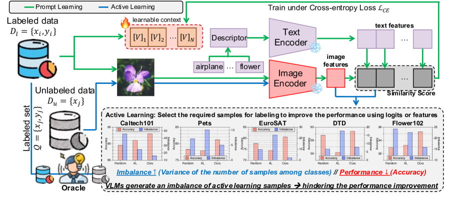
Figure 1: Key motivation and complete process behind active prompt learning. When we emply a traditional active learning framework for adapting prompt learning to a new target task, the active learning sampler incurs a significant imbalance (indicated by red bars). Thus, this imbalance results in an inability to enhance the ultimate performance (as indicated by blue bars). In this paper, we introduce a novel algorithm named PCB that rectifies this imbalance by harnessing the knowledge of VLMs, enabling effective utilization of the oracle.

Even though we can reduce the adpation cost, the barrier of high labeling costs still persists. To mitigate this inefficiency, there have been extensive studies in an area of active learning [49, 46]. The central objective of active learning is to select samples for labeling so that the model performance is significantly improved, and making a noticebale gap compared to random samples of the same quantity. These active learning methods can be roughly divided into two categories: (1) uncertainty-based sampling [10, 17, 23, 45, 16] and (2) diversity-based sampling [48, 41] which leverages feature embeddings from the image encoder. In a hybrid perspective, BADGE [2] was introduced by combining uncertainty and diversity through the use of $k$-means++ clustering within the gradient embedding space.

Under these two researches, our initial inquiry pertains to the determination of whether the implementation simply combining active learning with VLMs can effectively lead to enhanced classification performance. If it does not result in such improvement, what constitutes the critical incongruity in integrating these two methodologies? To address this question, we observe two phenomena: (1) naïvely applying active learning to VLMs does not consistently demonstrate improvements compared to random selection-based labeling (depicted as red bars in Figure 1); (2) this lack of improvement comes from the imbalanced class labels misled by an active learning framework (illustrated as blue bars in Figure 1). The imbalanced behavior of active learning algorithms is due to the imbalanced pre-trained knowledge of VLMs. We verify that pre-trained CLIP has different knowledge of each class by showing the class-wise accuracy (see Appendix A). Therefore, it is imperative to investigate how VLMs can effectively collaborate with active learning frameworks, particularly given that VLMs exacerbate the issue of class imbalance.

In this study, we introduce our approach, called PCB, which is designed to address the class imbalance issue and improve the classification performance of VLMs using only a limited amount of labeled data from experts. Our contributions are summarized as follows:

• This study represents the first exploration of synergistic approaches to active learning and VLMs, marking a novel contribution to the field. We establish that a straightforward combination of these two approaches does not consistently lead to an improvement, highlighting the need for enhacing active learning methods in this context.

• We delve into the underlying reasons for performance degradation of conventional active learning methods when combined with VLMs. Our investigation reveals that the selection of samples to be labeled by experts is imbalanced, thereby making VLMs biased.

• We introduce an algorithm named PCB, which harnesses the valuable pre-trained knowledge of VLMs to address the issue of class imbalance. This algorithm seamlessly integrates with conventional active learning techniques, resulting in a substantial enhancement of active prompt learning within VLMs.

2 Problem Formulation

2.1 Active Learning

The objective of active learning is to facilitate the learning of a multi-class classification model with $K$ classes while minimizing the labeling budget. The model undergoes an iterative training process through interactions with an oracle, who provides correct annotations. In each iteration, the model learns from an annotated dataset, denoted as $\mathcal{D}_{l}$$=\{(x_{i},y_{i})\}_{i=1}^{L}$, where $x_{i}\in\mathcal{X}$ is the input (e.g. images), and $y_{i}\in\{1,...,K\}$ is the corresponding label, and $L$ is the number of labeled samples. Upon sufficiently training the model with the given dataset $\mathcal{D}_{l}$, the active learning algorithm selects $N$ samples from the unlabeled dataset, $\mathcal{D}_{u}$. The oracle then provides the labels for these selected samples, and they are subsequently incorporated into the annotated dataset $\mathcal{D}_{l}$ for use in the training.

2.2 Vision Language Models and Prompt Learning

Vision language models (VLMs).  VLMs typically consist of two encoders: an image encoder and a text encoder. When presented with an image as an input, the image encoder transforms the image into an embedding vector. In the case of CLIP [44], one of the most representative VLMs, it employs the ResNet [14] and ViT [8] architectures as its image encoder. On the other hand, the objective of the text encoder is to map a sentence into an embedding vector with the same dimension as the output of the image encoder. CLIP employs the Transformer [53] architecture for its text encoder. The CLIP model is trained using an Image-Text constrastive loss to align the embeddings of image and text pairs, enabling it to learn meaningful associations between images and corresponding text descriptions.

Indeed, the classification process in the CLIP model relies on the similarity score between image and text pairs. Here is a summary of how the CLIP model performs classification. Given an image $x_{i}$, the embeddings for the image and text are formulated as

$$e_{\mathrm{img}}=\mathrm{CLIP_{img}}(x_{i}),\quad e_{\mathrm{txt}}^{k}=\mathrm{CLIP_{txt}}(T(\mathrm{CLS}_{k})).$$

Here, $T$ represents the text template (e.g. A photo of $\{\mathrm{CLS}_{k}\}$), and $\{\mathrm{CLS}_{k}\}$ denotes the class name of each class index $k\in\{1,2,...,K\}$. Using $e_{\mathrm{img}}$ and $e_{\mathrm{txt}}$, the prediction probability of each class $k$ is formulated as

$$\mathrm{P}(y=k|x)=\frac{\mathrm{exp}(\mathrm{cos}(e_{\mathrm{img}},e_{\mathrm{txt}}^{k})/\tau)}{\sum_{i=1}^{K}\mathrm{exp}(\mathrm{cos}(e_{\mathrm{img}},e_{\mathrm{txt}}^{i})/\tau)}$$

where $\tau$ represents a temperature parameter, and $\mathrm{cos(\cdot,\cdot)}$ is the cosine similarity.

Prompt learning (PL).  PL is an efficient adaptation method that allows partial parts of prompts to be trainable [63, 62, 21, 20, 34, 50, 19, 32, 61, 26, 12]. It improves performance by updating the following criteria. Suppose that the class name $\{\mathrm{CLS}\}$ is tokenized as $[\mathrm{CLS}]$, and the text template function $T$ generates tokens as follows:

$$T(\mathrm{CLS}_{k})=[V]_{1}[V]_{2}\ldots[V]_{M}[\mathrm{CLS}_{k}].$$

Here, $[V]_{i}$ represent trainable tokens, and $[\mathrm{CLS}_{k}]$ is a fixed token for each class name $\{\mathrm{CLS}_{k}\}$. Note that the position of trainable tokens can be changed, e.g. by placing them right after the class token; we simply notate it as the front case for simplification. These trainable parameters are trained using the cross-entropy loss function defined as

$$\mathcal{L}_{\text{CE}}(x_{i},y_{i})=-\sum_{k=1}^{K}\mathbbm{1}\{y_{i}=k\}\log P(y=k|x_{i}).$$

3 Method: PCB

As depicted in Figure 1, two key motivations can be derived: (1) the traditional approach to select unlabeled samples in active learning leads to an imbalance under pre-trained VLMs, and (2) achieving a balance is imperative for enhancing overall performance, but it is challenging with unlabeled data; it can rather cause deeper imbalance by using false knowledge. Building upon the insights from these findings, we recognize the significance of balancing in improving performance within the active prompt learning problem. To address this objective, we introduce a novel algorithm named PCB: Pseudo-Class Balance for Active Prompt Learning in VLMs. In the following section, we delve into a detailed explanation of the entire workflow encompassed by the proposed algorithm.

3.1 Pseudo-Class Balance for Active Prompt Learning in VLMs

Input: Labeled dataset $\mathcal{D}_{l}$, Pseudo-labeled dataset $\tilde{P}$, Budget $N$

Init: $\mathcal{Q}=\emptyset$ (Query set), $\tilde{\mathcal{D}}_{l}=\mathcal{D}_{l}$ (Estimated $\mathcal{D}_{l}$)

for $n=1,2,...,N$ do

       # Select class $k$, the smallest # of class samples in $\tilde{\mathcal{D}}_{l}$

       $k=\operatorname*{arg\,min}_{k\in\{1,...,K\}}|c_{k}|$

       where $c_{k}=\{(x_{i},y_{i})|y_{i}=k\,\text{and}\,(x_{i},y_{i})\in\tilde{\mathcal{D}}_{l}\}$

       # Select one sample pseudo-labeled as $k$ from $\tilde{P}$

       $(x_{j},\tilde{y}_{j})\in\tilde{P}$, where $\tilde{y}_{j}=k$

       # Update query set $\mathcal{Q}$ by adding the selected sample

       $\mathcal{Q}=\mathcal{Q}\cup[(x_{j})]$

       # Update estimated labeled set $\tilde{\mathcal{D}}_{l}$

       $\tilde{\mathcal{D}}_{l}=\tilde{\mathcal{D}}_{l}\cup[(x_{j},\tilde{y}_{j})]$

end for

Output: Query set $\mathcal{Q}$

Algorithm 1 Balance_sampler

Balance sampler.  To satisfy the class balance while selecting informative samples for improving ultimate performance, we propose the two-stage active learning method on VLMs. First, we select a subset of informative samples, $P\subset\mathcal{D}_{u}$ where the size of $P$ is $\gamma\times|\mathcal{D}_{u}|$. Here $\gamma\in[0,1]$ is the hyperparameter that controls how progressively allow the uncertain samples to be labeled. After selecting $P$, we pseudo-label the selected samples by using VLMs’ classification ability, i.e. $\tilde{P}=\{(x_{i},\tilde{y}_{i})\}_{i=1}^{\gamma|D_{u}|}$. Then, we build the query set $\mathcal{Q}$ by utilizing the balance sampler, as described in Algorithm 1, randomly selecting samples from $\tilde{P}$ so that the expected number of samples of each class is balanced.

1

Input: $\mathcal{D}_{l}$, $\mathcal{D}_{u}$, $R$, $N$, $\gamma$, $\mathcal{A}$, $\texttt{Oracle}(\cdot)$, $f$.

for $r=1,2,...,R$ do

       if $r=1$ then

             # Initial query set $\mathcal{Q}$

             $\mathcal{Q}=\texttt{random\_sample}(\mathcal{D}_{u},N)$

       end if

      else

             # Select informative subset $P$

             $P=\mathcal{A}(\mathcal{D}_{u},\gamma|\mathcal{D}_{u}|,f)$

             # Pseudo labeling

             $\tilde{P}=\{(x_{i},\tilde{y}_{i})|(x_{i},y_{i})\in\mathcal{D}_{u}\,\text{and}\,\tilde{y}_{i}=f(x_{i})\}$

             # Balance_sampler (Algorithm 1)

             $\mathcal{Q}=\texttt{Balance\_sampler}(\mathcal{D}_{u},\tilde{\mathcal{P}},N)$

       end if

      # Labeling by Oracle

       $\hat{\mathcal{Q}}=\{(x_{i},y_{i})|x_{i}\in\mathcal{Q}\,\text{and}\,y_{i}=\texttt{Oracle}(x_{i})\}$

       # Update both sets and train prompts (Section 3.2)

       $\mathcal{D}_{l}$ = $\mathcal{D}_{l}\cup\hat{\mathcal{Q}}$, $\mathcal{D}_{u}$ = $\mathcal{D}_{u}\backslash\mathcal{Q}$

       Train learnable prompts $[V]_{i}$ on $\mathcal{D}_{l}$

end for

Output: Final model $f$

Algorithm 2 PCB

Proposed method.  Based on the balancing module, we introduce a method called PCB, which is briefly outlined in Algorithm 2. This algorithm takes inputs as a labeled dataset $\mathcal{D}_{l}$, an unlabeled dataset $\mathcal{D}_{u}$, the number of active learning rounds $R$, a query budget $N$, a progressive hyperparameter $\gamma$, an active learning algorithm $\mathcal{A}$, an oracle labeler Oracle, and a VLM model $f$.

The initial round randomly selects a query set due to insufficient information about the target dataset. From the second round, an active learning algorithm builds an informative subset $P$ and assigns pseudo-labels to its samples. The Algorithm 1 then aims to create a balanced labeled dataset. After obtaining true labels for the query set $\mathcal{Q}$ from an oracle, the procedure proceeds to train the parameters $[V]_{i}$.

3.2 Description Augmentation

In order to improve the classification performance of VLM-based models, numerous studies have explored the integration of external knowledge, as demonstrated in previous research works [37, 42]. These studies have contributed to show how models (e.g. GPT-3 [4]) can help VLMs by generating visual description for each class. For instance, the authors of [37] introduced the following templates:

Q: What are useful features for distinguishing a {CLS} in a photo?

A: There are several useful visual features to tell there is a {CLS} in a photo:

where {CLS} indicates the class name. Here, note that we can obtain $\delta_{k}$ descriptions for class $k$, i.e. $\Delta_{k}=\{\mathrm{d}_{k}^{i}\}_{i=1}^{\delta_{k}}$, where $\mathrm{d}_{k}^{i}$ denote $i$-th description for class $k$.

By following the results of [37, 42], we adopt their prompts for training the model. In other words, we utilize the new text template function $T$ as follows:

Based on this new text template function, we can use two possible prediction probabilites.

(1) Average Similarity (AS):

$$\mathrm{P}(y=k|x)=\frac{1}{\delta_{k}}\sum_{i=1}^{\delta_{k}}\mathrm{P}(y=k|x,\mathrm{d}_{k}^{i}),$$

where

$$\mathrm{P}(y=k|x,\mathrm{d}_{k}^{i})=\frac{\mathrm{exp}(\mathrm{cos}(e_{\mathrm{img}},e_{\mathrm{txt}}^{k,i})/\tau)}{\sum_{i=1}^{K}\sum_{j=1}^{\delta_{k}}\mathrm{exp}(\mathrm{cos}(e_{\mathrm{img}},e_{\mathrm{txt}}^{k,i})/\tau)}.$$

(2) Average Embedding (AE):

$$\mathrm{P}(y=k|x)=\frac{\mathrm{exp}(\mathrm{cos}(e_{\mathrm{img}},e_{\mathrm{txt}}^{k})/\tau)}{\sum_{i=1}^{K}\mathrm{exp}(\mathrm{cos}(e_{\mathrm{img}},e_{\mathrm{txt}}^{i})/\tau)},$$

where

$$e_{\mathrm{txt}}^{k}=\frac{1}{\delta_{k}}\sum_{i=1}^{\delta_{k}}e_{\mathrm{txt}}^{k,i}.$$

Note that the primary distinction between two probability scores lies in their respective averaging timeframes. AS calcuates individual embeddings and then computes the average similarity, whereas AE first averages the embeddings and then assesses the similarity.

Final Accuracy ($\uparrow$) Method Flowers102 DTD Oxford Pets EuroSAT Caltech101 Stanford Cars Aircraft Avg Acc ($\uparrow$) CLIP (zero-shot) 66.7 44.5 87.0 49.4 87.9 59.4 21.2 59.44 Random 92.92$\pm$0.61 58.77$\pm$1.94 78.30$\pm$0.74 77.62$\pm$1.12 89.55$\pm$1.00 65.96$\pm$0.08 30.69$\pm$0.30 70.54 Entropy [16] 94.80$\pm$0.75 59.18$\pm$1.31 76.81$\pm$1.38 75.46$\pm$3.39 91.67$\pm$0.09 66.68$\pm$0.91 25.80$\pm$0.78 70.06 $~{}~{}+\mathrm{\texttt{PCB}}$ 96.16$\pm$0.45 59.73$\pm$1.96 80.44$\pm$1.24 80.80$\pm$2.88 92.41$\pm$0.50 67.18$\pm$0.28 26.78$\pm$0.87 71.93 $~{}~{}+\mathrm{\texttt{PCB}(\texttt{AE})}$ 96.33$\pm$0.06 60.07$\pm$1.69 80.87$\pm$0.60 81.72$\pm$0.53 93.14$\pm$0.51 66.42$\pm$0.86 27.09$\pm$0.13 72.23 $~{}~{}+\mathrm{\texttt{PCB}(\texttt{AS})}$ 96.94$\pm$0.19 59.50$\pm$1.99 80.94$\pm$1.05 80.75$\pm$1.15 93.48$\pm$0.26 68.93$\pm$0.86 27.58$\pm$0.43 72.59 Coreset [48] 88.65$\pm$0.68 50.39$\pm$0.54 76.70$\pm$0.52 68.09$\pm$1.54 88.78$\pm$0.49 61.75$\pm$0.60 24.32$\pm$0.45 65.53 $~{}~{}+\mathrm{\texttt{PCB}}$ 91.30$\pm$0.90 55.77$\pm$1.33 76.84$\pm$1.10 77.50$\pm$4.64 89.96$\pm$0.03 63.63$\pm$0.27 25.38$\pm$0.64 68.63 $~{}~{}+\mathrm{\texttt{PCB}(\texttt{AE})}$ 91.70$\pm$0.29 57.09$\pm$0.63 78.60$\pm$1.14 79.28$\pm$0.14 90.29$\pm$0.30 62.08$\pm$0.35 26.19$\pm$1.40 69.31 $~{}~{}+\mathrm{\texttt{PCB}(\texttt{AS})}$ 92.33$\pm$0.84 56.38$\pm$0.73 79.50$\pm$0.91 79.28$\pm$1.42 91.70$\pm$0.48 65.75$\pm$0.55 26.22$\pm$0.47 70.17 BADGE [2] 96.33$\pm$0.39 58.98$\pm$1.30 80.03$\pm$1.19 79.79$\pm$0.94 92.54$\pm$0.01 68.07$\pm$0.61 31.25$\pm$0.45 72.43 $~{}~{}+\mathrm{\texttt{PCB}}$ 96.12$\pm$0.12 60.28$\pm$0.75 80.22$\pm$1.69 81.98$\pm$0.81 92.21$\pm$0.92 68.50$\pm$0.26 31.35$\pm$0.21 72.95 $~{}~{}+\mathrm{\texttt{PCB}(\texttt{AE})}$ 96.35$\pm$0.27 61.92$\pm$1.60 81.93$\pm$0.88 80.70$\pm$3.67 92.52$\pm$0.32 67.70$\pm$0.84 31.80$\pm$0.08 73.27 $~{}~{}+\mathrm{\texttt{PCB}(\texttt{AS})}$ 96.71$\pm$0.29 62.33$\pm$1.06 83.16$\pm$0.18 81.50$\pm$1.11 93.85$\pm$0.37 70.70$\pm$0.79 32.27$\pm$0.66 74.36 Full data 97.9 74.7 89.3 94.5 94.4 80.8 43.4 82.14

Table 1: Final accuracy on seven downstream tasks with ViT-B/32 image encoder. Final Accuracy is the the accuracy after eight rounds, and Avg Acc is the average of final accuracies of seven datasets. AS and AE are the average score and the average embedding, respectively, as described in Section 3.2. Also, CLIP (zero-shot) is the accuracy of each task from pretrained CLIP as reported in [44], and Full data is the accuracy when exploiting the whole dataset while prompt learning. Please note that the bold type and underline type represent the best performance overall and within the same active learning, respectively.

4 Experiment

4.1 Implementation Details

Datasets.  For image classification in downstream tasks, we select seven openly available image classification datasets that have been previously utilized in the CLIP model [44], specifically EuroSAT [15], Oxford Pets [40], DTD [5], Caltech101 [9], Flowers102 [39], StanfordCars [25], and FGVC-Aircraft [35]. These benchmarks span diverse categories, encompassing classification tasks involving common objects, scenes, patterns, and fine-grained categories.

Training details.  Our active learning setup consists of eight rounds (i.e. $R$=8), and in each round, we select a subset whose size is the number of classes, i.e. $N$=$K$ . To serve as the backbone for our image encoder, we adopt ViT-B/32. The size of the context vectors $M$ is set to $16$, and they are initialized using a zero-mean Gaussian distribution with a standard deviation of $0.02$. Throughout the training process for all rounds, we employ the SGD optimizer with a learning rate $0.002$, which is decayed by the cosine annealing scheduler. We also set the maximum epoch as $200$. All methods are implemented with PyTorch 2.0.1 and executed on a single NVIDIA A5000 GPU.

Active learning methods.  To validate the effectiveness of PCB, we select three representative active learning methods: (1) Entropy [16] selects the most uncertain examples with the highest entropy value from logits in the prediction; (2) Coreset [48] queries the most diverse examples using embeddings from the model (i.e. image encoder); and (3) BADGE [2] considers both uncertainty and diversity by selecting the examples via $k$-means++ clustering in the gradient space. By adding PCB into those active learning methods, we study the synergy of active learning and PCB, and compare the results with random sampling (i.e. instead of active learning) and zero-shot CLIP. Furthermore, we show the results when using the descriptions presented in Section 3.2. To illustrate the room for performance enhancement, we also measure the performance when prompt learning the model with the whole dataset (see “Full data”).

Metrics.  To validate the effectiveness of our method, we use the final accuracy that indicates the accuracy at the last round. As in previous analysis about imbalance, we use the variance value of the number of samples among classes. Note that all experiments are conducted three times, and all the results are reported as averages.

4.2 Overall Results

Final Accuracy ($\uparrow$) Model Method Flowers102 DTD Oxford Pets EuroSAT Caltech101 Stanford Cars Aircraft Avg Acc ($\uparrow$) RN50 CLIP (zero-shot) 65.9 41.7 85.4 41.1 82.1 55.8 19.3 55.9 Random 92.06$\pm$0.54 56.62$\pm$0.97 74.65$\pm$0.50 79.10$\pm$2.31 84.11$\pm$0.75 61.34$\pm$0.57 29.15$\pm$0.32 68.18 BADGE [2] 95.56$\pm$0.54 58.35$\pm$1.20 75.06$\pm$0.50 80.94$\pm$0.55 89.67$\pm$0.30 63.96$\pm$0.53 28.12$\pm$1.03 70.24 $~{}~{}+\mathrm{\texttt{PCB}}$ 95.66$\pm$0.28 57.41$\pm$0.17 76.51$\pm$1.83 80.06$\pm$0.97 89.06$\pm$0.21 63.18$\pm$0.77 29.23$\pm$0.35 70.16 $~{}~{}+\mathrm{\texttt{PCB}(\texttt{AE})}$ 95.72$\pm$0.31 59.20$\pm$1.25 76.77$\pm$0.65 81.96$\pm$0.60 89.57$\pm$0.19 62.62$\pm$0.26 28.85$\pm$1.59 70.67 $~{}~{}+\mathrm{\texttt{PCB}(\texttt{AS})}$ 96.18$\pm$0.07 59.14$\pm$1.08 80.09$\pm$0.85 81.60$\pm$2.89 90.76$\pm$0.34 66.20$\pm$0.69 29.61$\pm$0.78 71.94 Full data 97.6 71.6 88.0 93.6 92.8 78.8 42.6 80.71 RN101 CLIP (zero-shot) 65.7 43.9 86.2 33.1 85.1 62.3 19.5 56.54 Random 92.87$\pm$0.43 58.29$\pm$1.24 79.08$\pm$1.39 77.21$\pm$4.13 87.55$\pm$0.75 70.02$\pm$0.36 32.76$\pm$0.29 71.11 BADGE [2] 96.26$\pm$0.07 59.93$\pm$1.25 80.77$\pm$1.31 78.23$\pm$2.22 91.35$\pm$0.32 71.43$\pm$0.97 32.56$\pm$0.64 72.93 $~{}~{}+\mathrm{\texttt{PCB}}$ 95.79$\pm$0.38 60.20$\pm$1.89 80.94$\pm$0.42 79.55$\pm$1.37 91.75$\pm$0.44 71.35$\pm$0.39 32.62$\pm$1.48 73.17 $~{}~{}+\mathrm{\texttt{PCB}(\texttt{AE})}$ 96.49$\pm$0.26 62.59$\pm$0.84 83.02$\pm$0.89 81.50$\pm$0.69 92.51$\pm$0.32 71.42$\pm$0.77 32.76$\pm$0.76 74.33 $~{}~{}+\mathrm{\texttt{PCB}(\texttt{AS})}$ 96.47$\pm$0.18 62.17$\pm$1.04 83.48$\pm$2.13 81.14$\pm$1.57 92.87$\pm$0.18 74.04$\pm$0.39 32.84$\pm$0.85 75.43 Full data 97.8 74.2 91.1 92.9 94.7 83.7 46.0 82.91 ViT-B/16 CLIP (zero-shot) 70.4 46.0 88.9 54.1 88.9 65.6 27.1 63.0 Random 94.98$\pm$0.06 62.63$\pm$1.81 84.36$\pm$1.34 81.14$\pm$1.83 90.95$\pm$0.85 73.62$\pm$0.30 38.88$\pm$0.25 75.22 BADGE [2] 97.97$\pm$0.41 62.84$\pm$2.17 85.54$\pm$1.30 82.22$\pm$1.94 93.77$\pm$0.51 76.55$\pm$0.78 39.64$\pm$0.14 76.93 $~{}~{}+\mathrm{\texttt{PCB}}$ 98.32$\pm$0.21 64.89$\pm$1.45 86.22$\pm$0.71 81.53$\pm$3.11 93.75$\pm$0.28 76.36$\pm$0.27 40.20$\pm$0.30 77.32 $~{}~{}+\mathrm{\texttt{PCB}(\texttt{AE})}$ 98.21$\pm$0.21 65.25$\pm$1.28 87.23$\pm$0.35 84.04$\pm$2.92 94.51$\pm$0.29 75.84$\pm$0.44 39.93$\pm$0.21 77.86 $~{}~{}+\mathrm{\texttt{PCB}(\texttt{AS})}$ 98.19$\pm$0.17 64.95$\pm$1.47 88.10$\pm$1.49 83.85$\pm$2.45 95.12$\pm$0.26 78.19$\pm$0.48 40.56$\pm$0.51 78.42 Full data 99.0 77.7 92.7 95.1 95.3 85.3 53.6 85.53

Table 2: Various architectures of image encoder. We report the performance on various types of architectures, such as ResNet-50/101 and ViT-B/16, under the BADGE active learning algorithm. The performance under Entropy and Coreset are described in Appendix E.

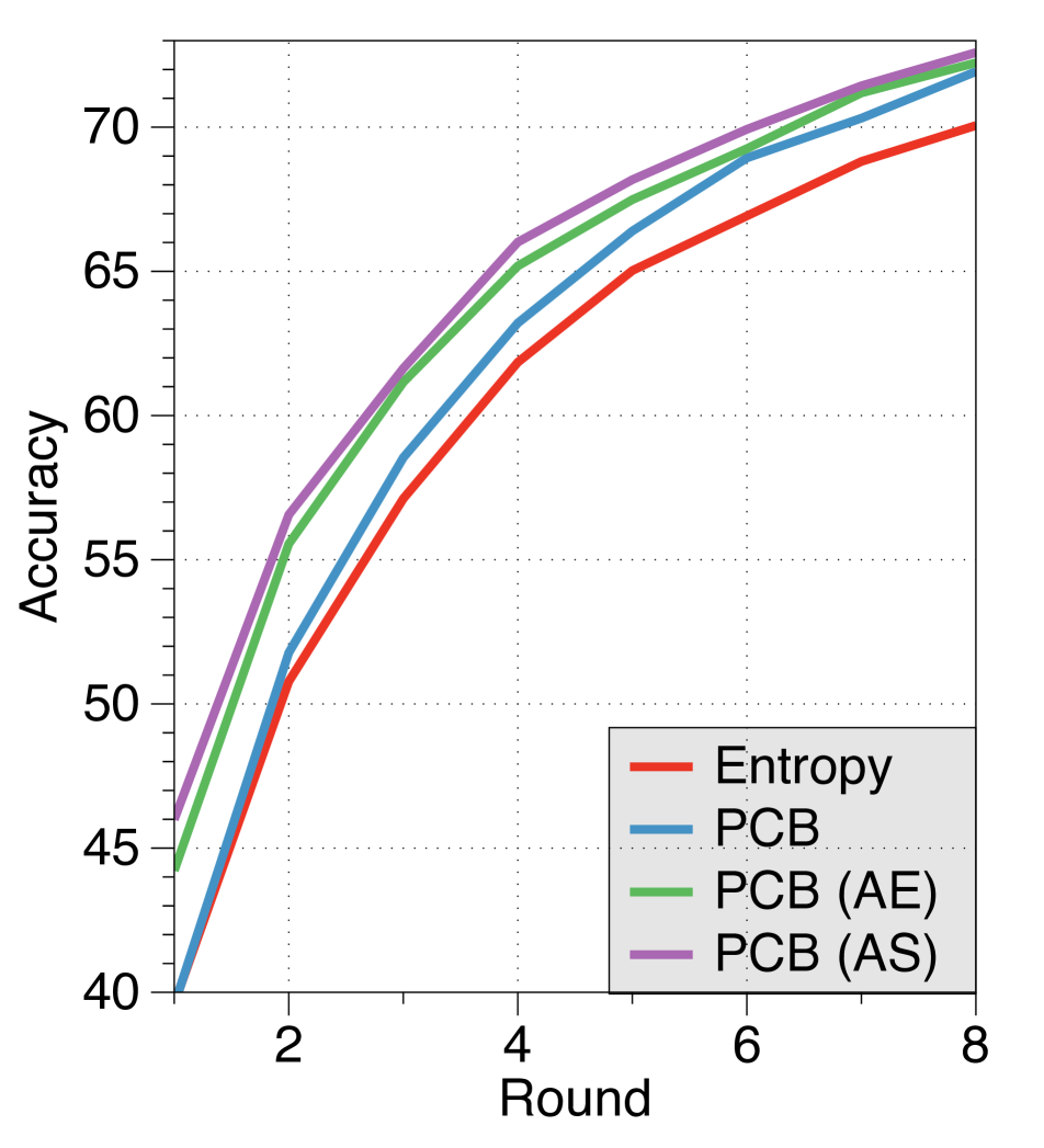
(a) Entropy

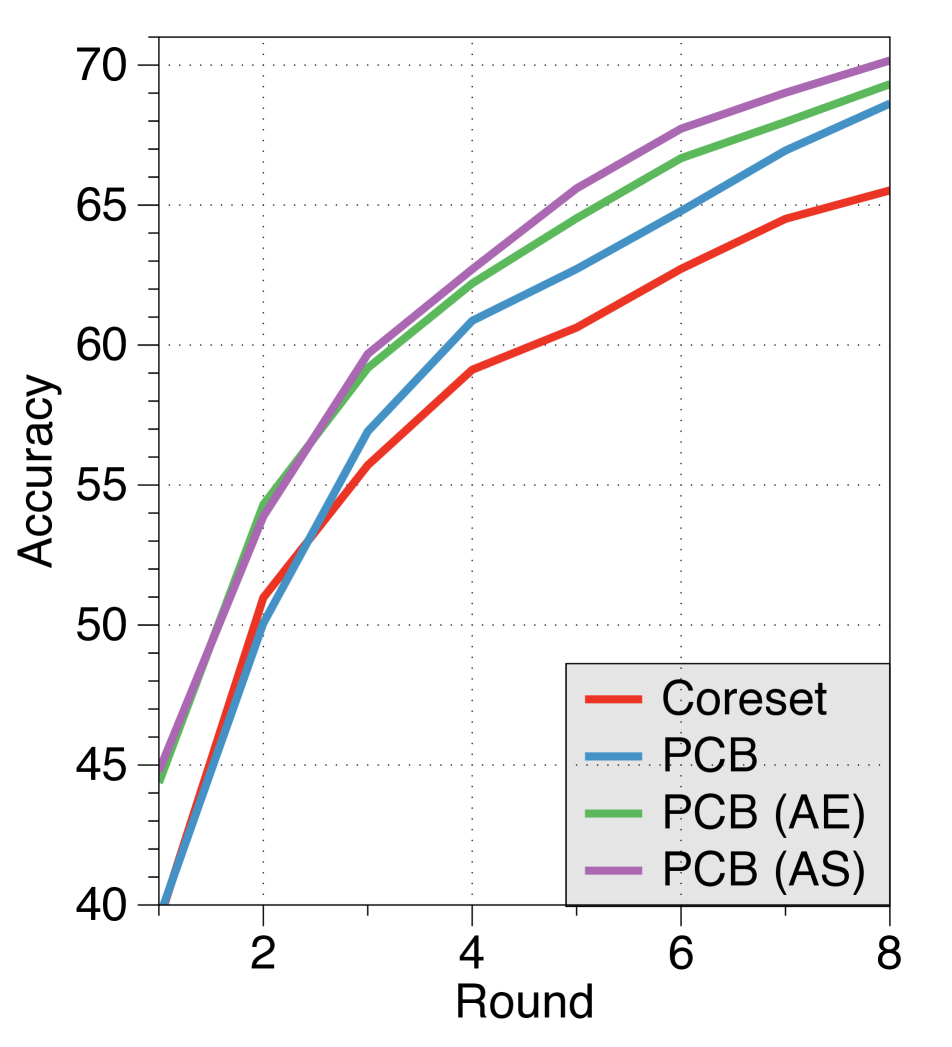
(b) Coreset

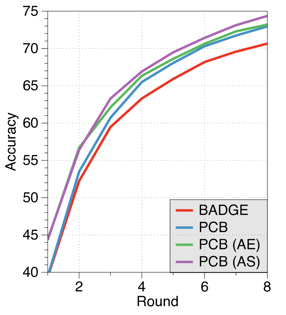
(c) BADGE

Figure 2: Learning curve. Average accuracy on downstream tasks with the ViT-B/32 image encoder for each round.

PCB improves performance.  We evaluate our methodology by integrating it with three active learning methods—Entropy, Coreset, and BADGE—and compare it with the Random approach and the pre-trained zero-shot CLIP model. As shown in Table 1, the proposed algorithm mostly improves performance in each case of its integration. For example, in the DTD dataset with the BADGE algorithm, applying PCB (AS) results in a $3.35\%$ improvement compared to the case without our algorithm. Furthermore, on average across datasets, leveraging our algorithm shows a performance improvement up to $4.64\%$. Additionally, across all active learning algorithms, PCB (AS) cases typically exhibit the highest accuracy.

Active learning can be poor than Random.  As shown in Table 1, active learning algorithms exhibit lower performance than the Random approach in some cases. For example, especially in EuroSAT and Aircraft, both Entropy and Coreset strategies perform worse than the Random approach, because these active learning algorithms select imbalanced datasets for labeling, leading to performance degradation. See Appendix A for the detailed evidences.

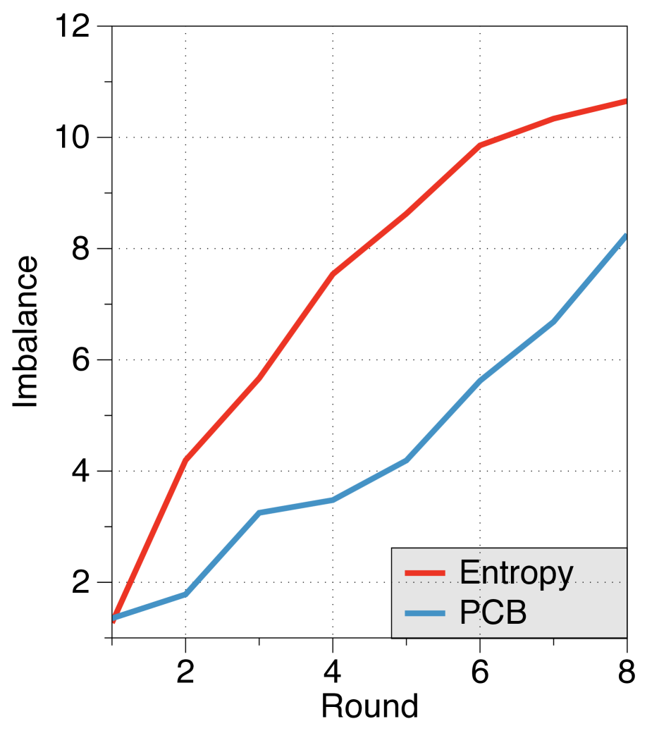
(a) Entropy

(b) Coreset

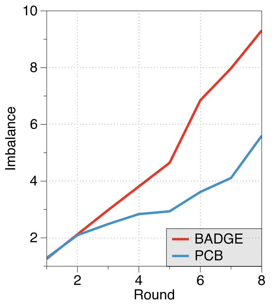
(c) BADGE

Figure 3: Imbalance curve. Average variance of the number of labeled samples for each class on downstream tasks with the ViT-B/32 image encoder for each round.

Learning curve.  Figure 2 illustrates the learning curve of the avearge accuracy among various datasets for each algorithm with or without the proposed algorithm. In all cases, applying PCB with AS shows the best performance. Furthermore, utilizing PCB improves the performance compared to the active learning algorithms without PCB. In particular, all figures represent that applying PCB demonstrates an increasing gap between with PCB and without PCB as the training progresses. It indicates that, based on our imbalance analysis described in Figure 3 and detailed in Appendix A, reducing the imbalance when constructing the query set $\mathcal{Q}$ is crucial in active prompt learning.

Additional analysis.  In the case of Oxford Pets, PCB exhibits lower performance than CLIP (zero-shot). This result is consistent with the results from the original CoOp paper [63]. To further analyze this phenomenon, we increase the number of samples (i.e. $N$) selected at each round by the active learning algorithm from $K$ to $16K$. When $N$=$4K$, PCB combined with BADGE outperforms zero-shot CLIP, and detailed results are described in Appendix D. We can conclude that the reason of performance degradation in Oxford Pets is due to the lack of samples involved in training.

4.3 Detailed Analyses

In this section, we answer the following questions: (1) other architectures of the image encoder in the CLIP family, (2) class imbalance analysis over different $\gamma$ values, (3) analysis on various prompt learning methods, and (4) hyperparameter sensitivity analysis.

Other types of image encoder.  We assess the efficacy of our method across various image encoder models, as described in Table 2. Given the superior performance of PCB coupled with BADGE, as evidenced in Table 1, our subsequent analysis in Table 2 is confined to this particular setup. Our method shows a similar trend across different encoder architectures, as supported by these observations: (1) the accuracy of zero-shot CLIP can be significantly enhanced with finetuning randomly sampled data, (2) the combination of BADGE with PCB yields better results than random sampling, and (3) description augmentation (i.e. AS and AE) noticeably enhances the accuracy. Regardless of the encoder used, the overall accuracy increases, with the difference between AS and AE decreasing as the model size grows.

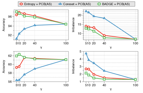
Figure 4: Accuracy and imbalance in terms of various $\gamma$ on Flowers102 (Upper) and DTD (Bottom).

Class imbalance analysis over different $\gamma$.   We also study the effectiveness of our method as $\gamma$ increases and summarize the results in terms of accuracy and imbalance in Figure 4. As shown in the figure, the accuracy increases as the imbalance decreases. In particular, Coreset+PCB (AS) has higher accuracy and lower imbalance as the $\gamma$ increases due to a larger number of unlabeled examples to balance classes. On the contrary, it is noteworthy that the accuracies of Entropy+PCB (AS) and BADGE+PCB (AS) do not tend to improve as $\gamma$ increases despite of more unlabeled samples for balancing. It indicates that getting informative (i.e. uncertain) data is very important to improve the accuracy after achieving a certain level of balance.

Moreover, we compare the accuracies and imbalances on two different datasets: Flowers102, which lacks class balance, and DTD, which exhibits class balance. As shown in Figure 4, the value of imbalance in Flowers102 is larger than that in DTD. More interestingly, in Flowers102, the imbalance value drops most dramatically in the range of 20%–40% of $\gamma$, whereas in DTD, the imbalance value drops most dramatically in the range of 10%–20% of $\gamma$. This indicates that achieving a class balance is obviously harder in an imbalanced dataset than in a balanced dataset.

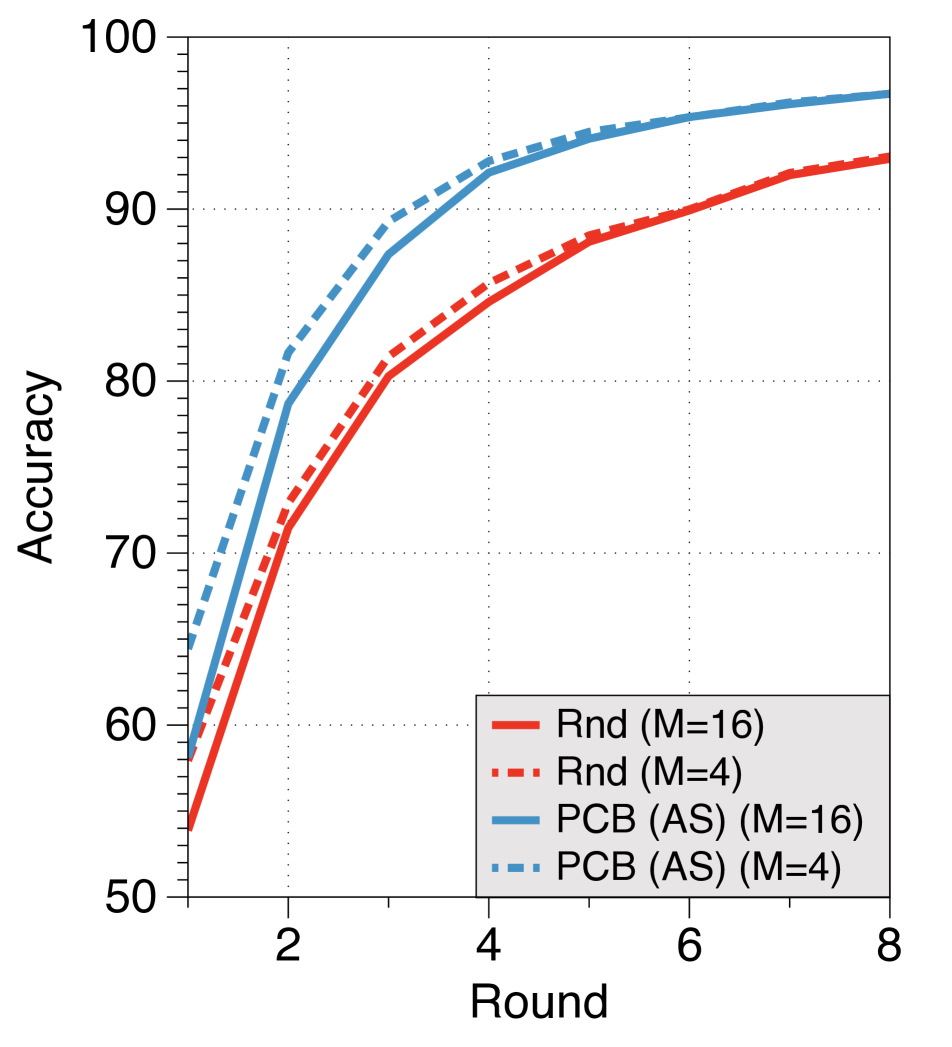
(a) Prompt Size $M$

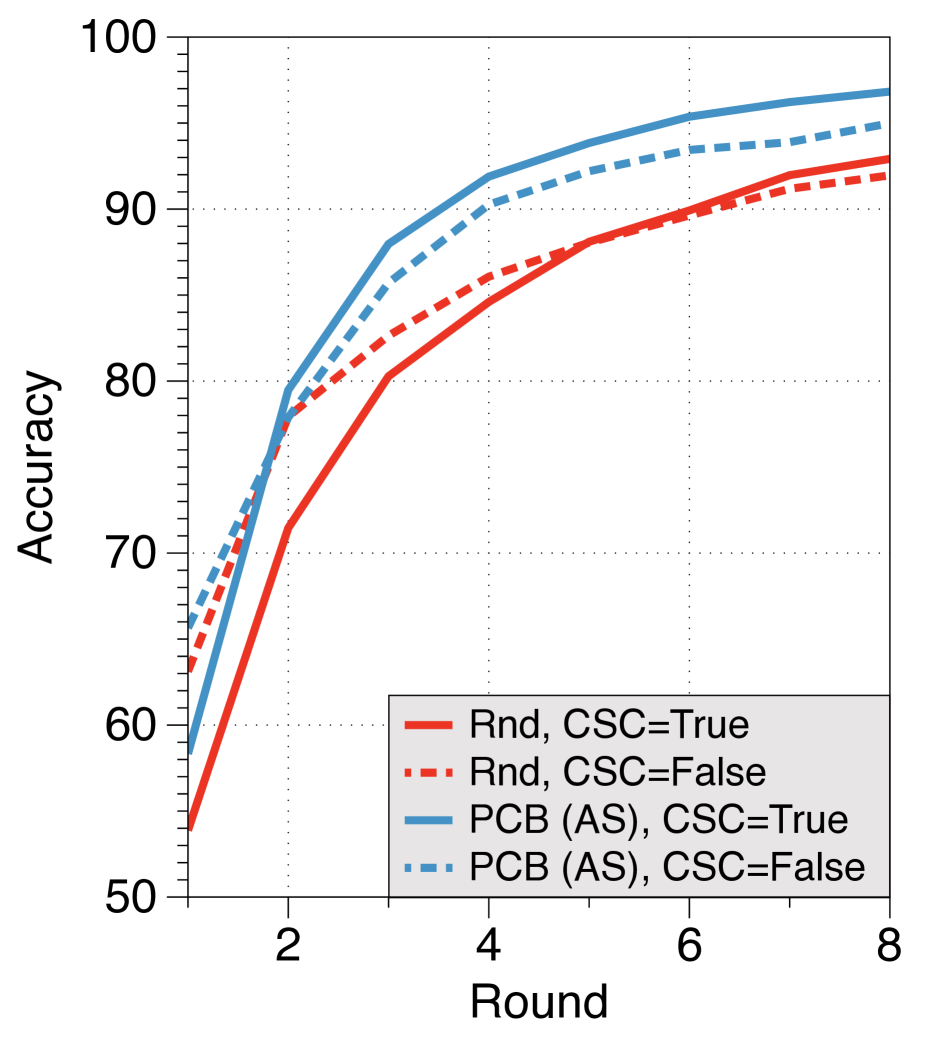
(b) CSC

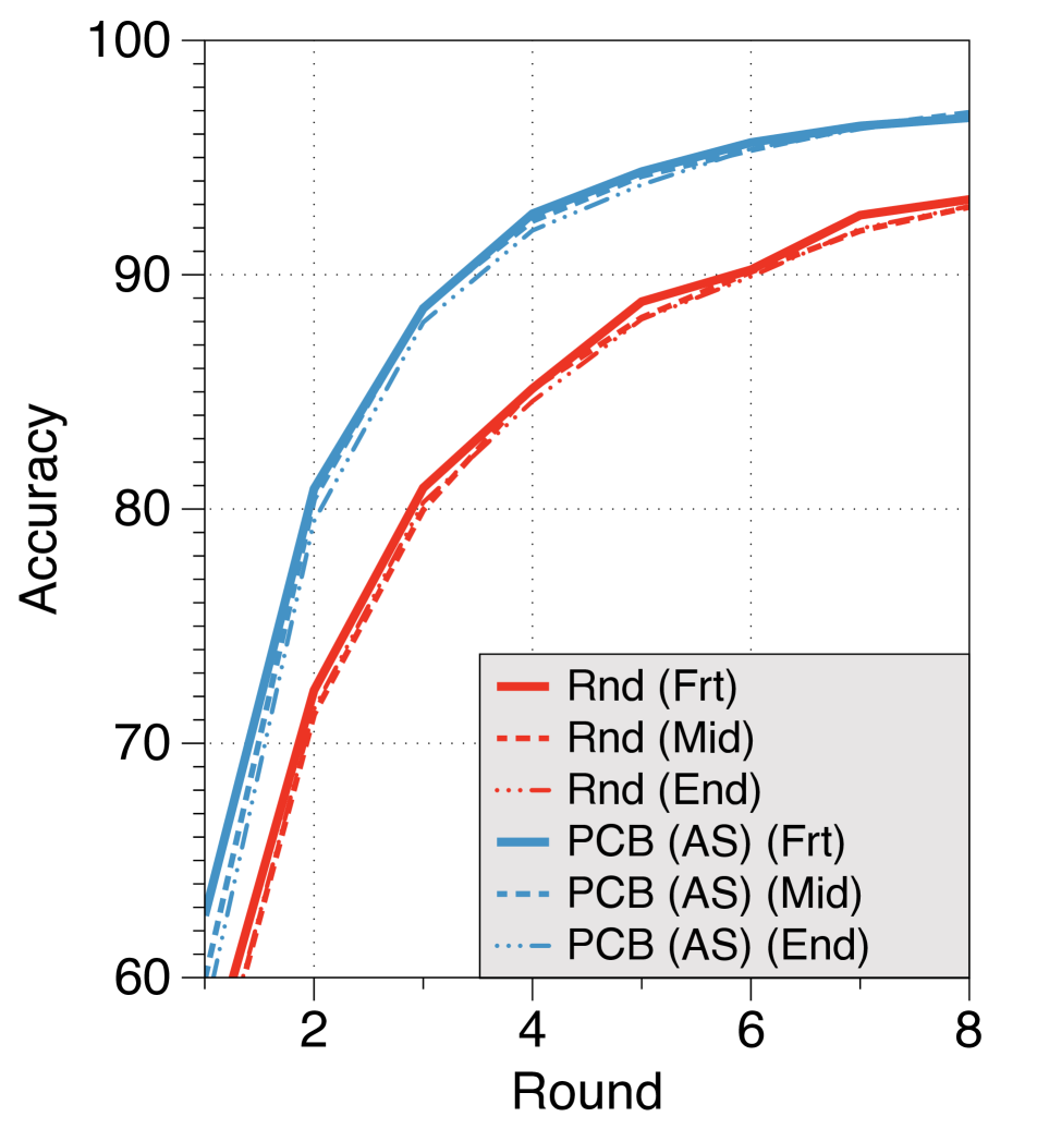
(c) Prompt Position

Figure 5: CoOp case analysis of BADGE on Flowers102.

Hyperparameter sensitivity.   We examine various variants of CoOp training methods, including different prompt sizes ($M$), cases where class-wise different tokens are not allowed (CSC=False), and variants in the position of trainable parameters (Front, Middle, and End).

In 5(a), it is observed that the accuracy with a small $M$ is higher than that with a large $M$, but this gap decreases as the rounds progress. Since the number of trainable parameters with a large $M$ is greater than that with a small $M$, the model with a large $M$ can be easily overfitted by a small labeled dataset at the initial round.

We analyze the performance gap when context vectors are shared for all classes (i.e. CSC=False) versus when different context vectors are used per class (i.e. CSC=True), and report the results in 5(b). The accuracy is shown to be initially higher when CSC=False, but it is beaten by CSC=True as the rounds progress. This phenomenon is attributed to the difference in the number of trainable parameters simlarly to 5(a).

Last, we measure the accuracy by changing the position of context vectors: Front (Frt), Middle (Mid), or End. As shown in 5(c), the accuracies with the Front position of context vectors are slightly better than those with the others over all rounds, but the gap is within the standard deviation. As such, it is hard to conclude that the position of context vectors affects the performance in active learning.

Visual Text Method $N$ PCB Entropy Coreset BADGE RN50 None LP 102 ✗ 79.78$\pm$1.01 70.66$\pm$1.16 81.23$\pm$0.40 FFT 102 ✗ 47.67$\pm$1.08 48.19$\pm$2.35 53.43$\pm$0.61 FFT 250 ✗ 77.48$\pm$3.45 78.91$\pm$0.77 79.51$\pm$0.32 Transformer CoCoOp [62] 102 ✗ 74.54$\pm$1.28 71.58$\pm$0.73 78.60$\pm$0.52 CoOp [63] 102 ✗ 94.74$\pm$0.40 85.61$\pm$1.36 95.56$\pm$0.54 Transformer CoCoOp [62] 102 $\mathcal{O}$ 76.18$\pm$1.55 72.74$\pm$1.29 80.06$\pm$1.53 CoOp [63] 102 $\mathcal{O}$ 95.89$\pm$0.32 91.34$\pm$1.00 95.66$\pm$0.28 ViT-B/32 None LP 102 ✗ 94.19$\pm$0.77 86.76$\pm$0.55 95.57$\pm$0.15 FFT 102 ✗ 37.01$\pm$1.69 35.90$\pm$1.26 43.14$\pm$0.89 FFT 250 ✗ 58.21$\pm$2.89 58.63$\pm$2.87 60.10$\pm$0.47 Transformer CoCoOp [62] 102 ✗ 76.41$\pm$1.29 73.54$\pm$0.68 78.94$\pm$0.36 MaPLe [21] 102 ✗ 84.72$\pm$2.56 80.98$\pm$0.80 87.86$\pm$1.84 CoOp [63] 102 ✗ 94.80$\pm$0.75 88.65$\pm$0.68 96.33$\pm$0.39 Transformer CoCoOp [62] 102 $\mathcal{O}$ 77.28$\pm$1.71 73.91$\pm$0.97 80.39$\pm$0.48 MaPLe [21] 102 $\mathcal{O}$ 87.60$\pm$1.93 82.51$\pm$0.22 88.14$\pm$0.73 CoOp [63] 102 $\mathcal{O}$ 96.16$\pm$0.45 91.30$\pm$0.90 96.12$\pm$0.12 ViT-B/16 Transformer CoCoOp [62] 102 ✗ 84.62$\pm$1.95 78.44$\pm$1.91 86.85$\pm$1.21 MaPLe [21] 102 ✗ 92.66$\pm$1.20 85.54$\pm$1.73 93.29$\pm$0.39 CoOp [63] 102 ✗ 97.32$\pm$0.23 92.22$\pm$2.03 97.97$\pm$0.41 Transformer CoCoOp [62] 102 $\mathcal{O}$ 85.61$\pm$1.63 80.44$\pm$0.56 87.41$\pm$1.42 MaPLe [21] 102 $\mathcal{O}$ 93.72$\pm$0.95 87.58$\pm$0.48 93.34$\pm$1.02 CoOp [63] 102 $\mathcal{O}$ 97.75$\pm$0.08 94.79$\pm$0.31 98.32$\pm$0.21

Table 3: Results of various training methods on Flowers102.

Various prompt learning methods.  There have been various types of prompt learning algorithms. Specifically, CoCoOp [62] and MaPLe [21] are popular among recent approaches, and they mainly focus on transferring to unseen novel classes. We evaluate the Flower102 performance of PCB and active learning algorithms on these other prompt learning algorithms, even though they do not mainly target the case where all classes are visible at the training pahse. Furthermore, we examine the performance of full fine-tuning (FFT), which tunes all parameters and place a linear classifier on top of the model, and linear probing (LP), which trains the linear layer to adapt to the new task.

First of all, without considering transferability, i.e. CoCoOp and MaPLe, CoOp shows better performance than LP and FFT. Also, we observe that the performance of CoCoOp and MaPLe is lower than that of CoOp. This observation aligns with the results reported in each paper, specifically concerning the base class performance, which pertains to the seen class during the training phase. Regardless of their performance superiority, when we compare the performance of ✗ and $\mathcal{O}$ indicating the setups without and with PCB, we find that PCB consistently improves performance. For instance, in the case of CoCoOp ViT-B/32, it enhances performance by $1.45\%$ point.

More precisely, we can conclude that FFT exhibits lower performance in a few-shot case. This phenomenon has also been reported in previous work [62], and we can attriute it to the few-shot training, as evidenced by the performance increase when we increase the number of samples from $102$ to $250$. However, it performs less effective than CoOp, indicating that prompt learning is superior to adaptation for new tasks in a few-shot perspective. Furthermore, PCB further enhances this improvement in an active learning setting.

5 Related Work

Vision language models (VLMs).  To comprehend the visual and language representations, multiple approaches have been explored [33, 6, 7, 43, 11, 56, 28]. In the stream of trials to understand both modalities at once, several years ago, CLIP [44] emerged, drawing significant attention due to its remarkable zero-shot performance across various tasks. In a similar vein, ALIGN [18] was introduced, employing a comparable training methodology but featuring distinct architectural and training dataset characteristics. Unlike CLIP, ALBEF [29] introduced multi-modal transformer operations applied to the outputs of two separate image and text encoders. BLIP [30] introduced a captioning module aimed at improving model performance by rectifying noisy captions. LiT [60] and BLIP-2 [31] enhanced training efficiency by freezing specific encoder parameters. The authors of FILIP [55] endeavored to enable the model to discern finer image details through a fine-grained, i.e. patch-level, matching training approach. Florence [58], on the other hand, sought to expand representations from various perspectives, such as image-to-video and so on.

Prompt learning in VLMs.  In the realm of natural language processing, there has been numerous works [50, 19, 32, 61, 26, 12, 21] aimed at enhancing the performance of language models through the optimization of prompts. The primary motivation behind these works lies in the huge size of models for fine-tuning, and it is also prevalent in the VLM area. Consequently, a considerable amount of research has been dedicated to prompt learning as a means to enhance classification accuracy. CoOp [63] is one of representative methods and has demonstrated that a minimal number of trainable parameters suffice to adapt to a given classification task. The authors of [34] introduced a methodology that leverages estimated weight distributions to assign weights aimed at minimizing classification errors.

Within this framework, several studies have aimed to enhance the generalization performance in prompt learning for VLMs [62, 57, 21, 22]. The primary task of these studies is to showcase a small number of classes and evaluate unseen ones. The same authors in [63] introduced CoCoOp [62], which incorporates a meta-network module to improve transferability. In the work presented in [57], the authors elucidated transferability in prompt learning from a VLM perspective. Moreover, MaPLe [21], a branch-aware hierarchical prompt method, was proposed where prompts for the image encoder are influenced by prompts for the text encoder. In PromptSRC [22], the authors highlight that previous prompt learning methods have overlooked the forgetting phenomenon during prompt training and propose an alignment-based self-regularization method to enhance transferability. It is noteworthy that this paper primarily focuses on active learning not for generalizability to new classes but for enhanced performance on the given task.

Description augmentation.  Recently, generating descriptions using large language models (LLMs) has gained popularity, owing to the significant improvements in the performance of VLMs. To generate descriptions for each specific class, we asked the questions based on the specific prompt template to the LLMs. A method was proposed by [37], where the scores obtained from different descriptions of the same class were averaged. In contrast, [42] proposed a method that utilized the averaged embeddings from multiple descriptions for each class.

Active learning.  Active learning [49, 46, 13, 38] aims to minimize human labeling costs by identifying informative data to maximize model performance. Most of the work has generally progressed along two trajectories: (1) uncertainty-based sampling and (2) diversity-based sampling. In uncertainty-based sampling, prediction probability-based sampling methods such as soft-max confidence [27], margin [47], and entropy [16] were simple yet effective. In addition, some methods performed multiple forward passes to achieve uncertainty. An intuitive approach was to receive the outputs from multiple experts [36, 24, 3]. Some methods [10, 17, 23] leveraged the Monte Carlo Dropout, which obtains the stochastic results from the same model using dropout layer. On the other hand, diversity-based sampling methods [48, 41] were introduced using either clustering or coreset selection protocols. The coreset method [48] identified sets of examples with the greatest coverage distance across all unlabeled data. More recently, hybrid methods leveraging both uncertainty and diversity have emerged. One such method, BADGE [2], employed $k$-means++ clustering within the gradient embedding space.

6 Conclusion

In this paper, we delve into the realm of active prompt learning within vision-language models (VLMs). Initially, we observe a misalignment between previous active learning algorithms and VLMs due to the inherent knowledge imbalance of VLMs. This imbalance consequently leads to a class imbalance of queried samples during the active learning process. To address this challenge, we introduce a novel algorithm named PCB which rectifies this imbalance by leveraging the knowledge embedded in VLMs before soliciting labels from the oracle labeler. Through extensive experiments across a range of real-world datasets, we demonstrate that our algorithm outperforms conventional active learning methods and surpasses the performance of random sampling. We believe that this framework opens up new avenues for research in the field of active learning within VLMs.

Acknowledgement.  This work was supported by Institute of Information & Communications Technology Planning & Evaluation (IITP) grant funded by the Korea government (MSIT) (No. 2020-0-00862, DB4DL: High-Usability and Performance In-Memory Distributed DBMS for Deep Learning and No. 2022-0-00157, Robust, Fair, Extensible Data-Centric Continual Learning).

 
-Supplementary Material-
Active Prompt Learning in Vision Language Models
 

This supplementray material presents additional analysis and explanation of our paper, “Active Prompt Learning in Vision Language Models”, that are not included in the main manuscript due to the page limitation. Appendix A analyses the reason why VLMs make imbalance during the active learning pipeline. Appendix B describes the detail experimental settings such as datsets and active learning baselines. Appendix C addresses the method details to generate the descriptions of each class. Since PCB indicates lower performance than zero-shot pretrained CLIP, we address this phenomenon in  Appendix D. Lastly,  Appendix E describes the additional results under not only BADGE active learning algorithm but also Entropy and Coreset algorithms with various architectures of an image encoder.

Flowers102 DTD Oxford Pets EuroSAT Caltech101 Stanford Cars Aircraft Method Acc Imbal Acc Imbal Acc Imbal Acc Imbal Acc Imbal Acc Imbal Acc Imbal CLIP (zero-shot) 66.7 - 44.5 - 87.0 - 49.4 - 87.9 - 59.4 - 21.2 - Random 92.92 24.31 58.77 6.77 78.30 7.17 77.62 9.50 89.55 48.52 65.96 8.09 30.69 6.02 Entropy [16] 94.80 20.54 59.18 6.64 76.81 7.31 75.46 10.87 91.67 15.03 66.68 10.69 25.80 17.11 $~{}~{}+\mathrm{\texttt{PCB}}$ 96.16 13.41 59.73 5.62 80.44 3.01 80.80 2.40 92.41 9.83 67.18 7.75 26.78 11.75 $~{}~{}+\mathrm{\texttt{PCB}(\texttt{AE})}$ 96.33 14.86 60.07 6.34 80.87 4.85 81.72 2.53 93.14 12.16 66.42 10.13 27.09 12.38 $~{}~{}+\mathrm{\texttt{PCB}(\texttt{AS})}$ 96.94 13.59 59.50 4.94 80.94 2.76 80.75 3.93 93.48 11.47 68.93 9.34 27.58 14.23 Coreset [48] 88.65 30.72 50.39 39.92 76.70 18.58 68.09 37.87 88.78 48.52 61.75 24.53 24.32 21.58 $~{}~{}+\mathrm{\texttt{PCB}}$ 91.30 21.24 55.77 15.50 76.84 8.74 77.50 2.07 89.96 22.08 63.63 13.44 25.38 14.27 $~{}~{}+\mathrm{\texttt{PCB}(\texttt{AE})}$ 91.70 21.59 57.09 16.34 78.60 8.97 79.28 1.00 90.29 20.33 62.08 14.38 26.19 14.27 $~{}~{}+\mathrm{\texttt{PCB}(\texttt{AS})}$ 92.33 21.50 56.38 14.98 79.50 9.86 79.28 1.13 91.70 22.11 65.75 12.51 26.22 13.74 BADGE [2] 96.33 17.89 58.98 5.90 80.03 5.71 79.79 5.47 92.54 13.19 68.07 5.77 31.25 6.87 $~{}~{}+\mathrm{\texttt{PCB}}$ 96.12 13.07 60.28 5.39 80.22 1.51 81.98 1.73 92.21 11.73 68.50 4.91 31.35 6.46 $~{}~{}+\mathrm{\texttt{PCB}(\texttt{AE})}$ 96.35 12.69 61.92 4.56 81.93 2.45 80.70 1.20 92.52 12.77 67.70 4.94 31.80 6.04 $~{}~{}+\mathrm{\texttt{PCB}(\texttt{AS})}$ 96.71 12.47 62.33 3.55 83.16 2.43 81.50 1.47 93.85 12.54 70.70 4.52 32.27 4.98 Full data 97.9 - 74.7 - 89.3 - 94.5 - 94.4 - 80.8 - 43.4 -

Table 4: Final accuracy and imbalance on seven downstream tasks with ViT-B/32 image encoder.

Appendix A Why Imbalane Occurs in VLMs

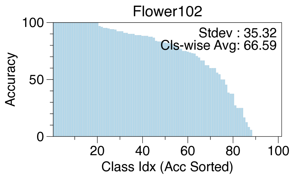
(a) Flower102

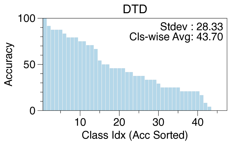
(b) DTD

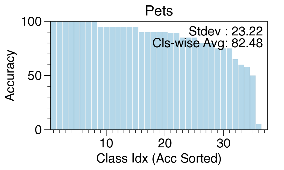
(c) Pets

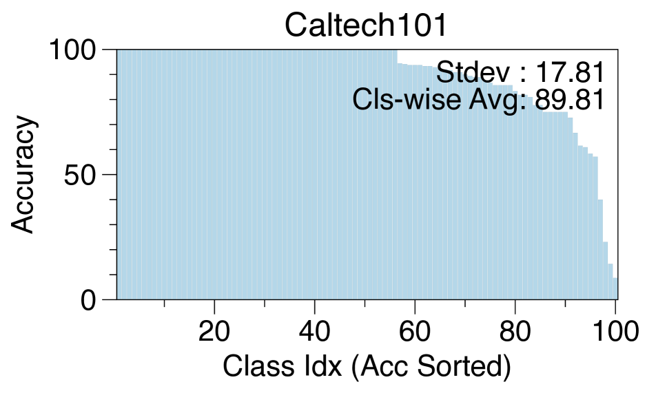
(d) Caltech101

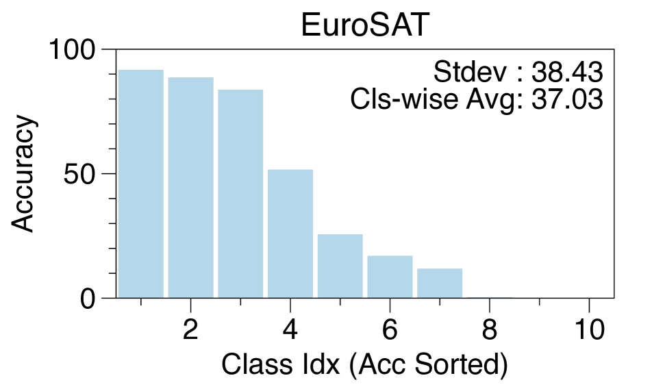
(e) EuroSAT

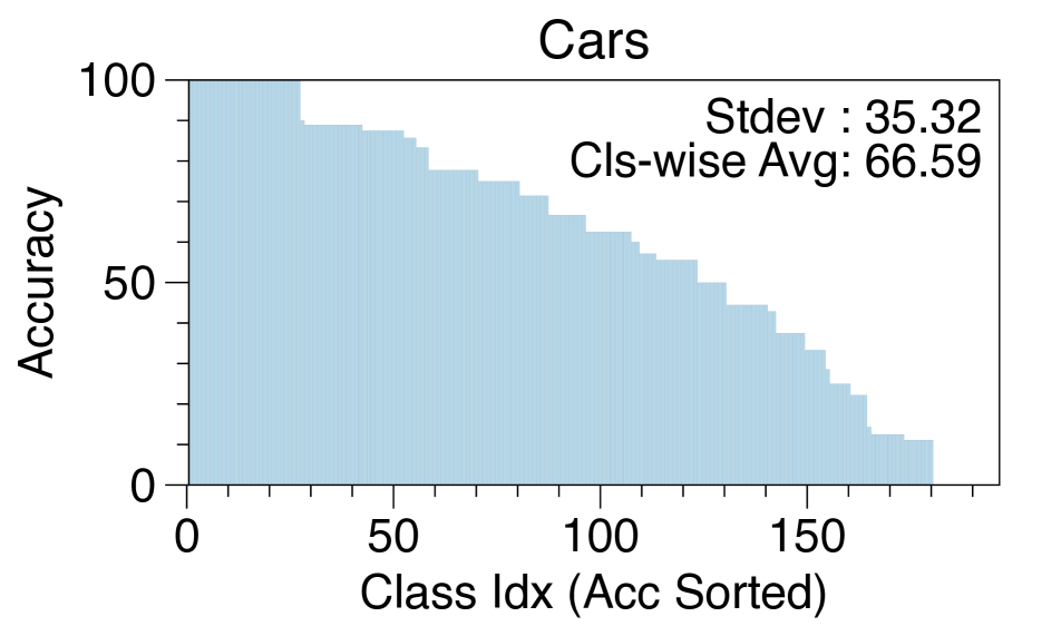
(f) Cars

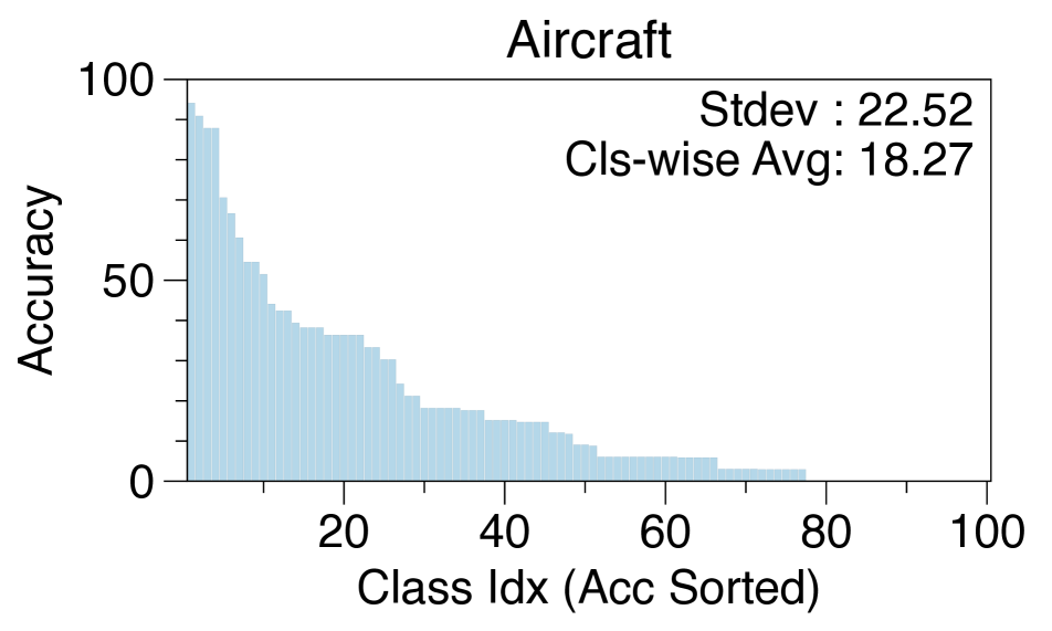
(g) Aircraft

Figure 6: Per class zero-shot accuracy from the pretrained CLIP with ViT-B/32 image encoder for each dataset.

Biased knowledge of pretrained CLIP.  Figure 6 indicates the zero-shot accuracy of each class when using pretrained CLIP for all the datasets. While pretrained CLIP has powerful knowledge for some classes, it has weakness for the other classes. For instance, in the case of Flowers102, pretrained CLIP has no knowledge in terms of stemless gentian by showing zero accuracy. On the contrary, it has perfect knowledge about moon orchid by indicating 100% point accuracy. As such, we can conclude that imbalanced knowledge of the pretrained CLIP causes imbalanced querying by active learning algorithms.

Imbalanced dataset degrades the performance.  Table 4 illustrates both accuracy and imbalance of labeled dataset after final round. For Oxford Pets, Stanford Cars, and FGVC aircraft datasets, where active learning algorithms can be poor than random sampling, the imbalances of Entropy and Coreset are higher than that of random sampling. It indicates that the large imbalance degrades the performance evenif they consist of uncertain or diversified data. As described in Section 4.3, Table 4 also shows that getting informative data enhances the accuracy after achieving a certain level of balance. For instance, despite the imbalance of BADGE being greater than that of Coreset paired with the PCB, the accuracy of the combination of Coreset and PCB is still lower than that of BADGE without PCB.

Appendix B Experimental Settings

Datasets.  We select seven openly available image classification datasets that have been previous utilized in the CLIP model. Here are the details of each dataset:

• Flowers102 [39] consists of 102 different categoris of flowers, each representing a distinct flower species. For example, it includes roses, sunflowers, daisies, and so on. The total number of 8,189 image and label pairs. Some categories have more images than the others, which means it is imbalanced as typical real-world datasets, at least 40 and at most 258 samples.

• DTD [5], abbreviated from Describable Texture Dataset, is designed for texture classification task. This dataset consists of 47 distinct classes, including categories like fabrics and natural materials. In total, DTD comprises 5,640 samples. Notably, when examining the performance reported in the CLIP [44], it becomes evdient that DTD poses a challenging problem for pre-trained CLIP models, as texture are not typical, easily recognizable objects.

• Oxford Pets [40] dataset consists of 37 different pet categories, including various dogs and cats. This dataset contains 7,400 samples. Especially, it has 4,978 dog images and 2,371 cat images. We utilize class labels even though the dataset has segmentation, i.e. RoI, and class both of them.

• EuroSAT [15] comprises 10 distinct classes that represent various land use and land cover categories. In total, this dataset includes 27,000 satelite images, with 2,700 images allocated to each of the 10 classes. Notably, each class contains an equal number of images, ensuring a balanced distribution within the dataset.

• Caltech101 [9] is composed of 101 unique object categories, each corresponding to a different type of object or scene. These categories encompass a wide range of objects, such as various animals, vehicles, and more. The dataset comprises a total of 9,000 images with varying numbers of images allocated to each category. Notably, Caltech-101 is considered a severely imbalanced dataset due to the uneven distribution of images across its categories.

• Stanford Cars [25] consists of a collection of 16,185 images categorized into 196 different classes, with each class typically representing a specific car make, model, and year, e.g. 2012 Tesla Model S, or 2012 BMW M3 Coupe.

• FGVC-Aircraft [35] encompasses a total of 10,200 images depicting various aircraft. This dataset is organized into 102 distinct classes, and each class corresponds to a specific aircraft model variant. Notably, there are 100 images available for each of these 102 different aircraft model variants. The class name in this dataset are composed of the make, model and specific variants such as Boeing 737-76J.

Active learning methods.  To validate the effectiveness of PCB, we select three representative active learning methods:

1. Entropy [16] selects the most uncertain examples with the highest entropy value from logits in the prediction. Specifically, selected query set $\mathcal{Q}$ with size $d$ is defined as follows:

   $$\mathcal{Q}=\operatorname*{arg\,max}_{Q\subset\mathcal{D}_{u},|Q|=d}\sum_{x_{i}\in Q}\mathcal{H}\left(f(x_{i})\right),$$

   where $\mathcal{H}(f(x))$ denotes entropy of softmax output $f(x)$.

2. Coreset [48] queries the most diverse examples using embeddings from the model (i.e. image encoder). More precisely, coreset is the problem that select the example that is the least relevant to the queried dataset. To solve it, the authors proposed $K$-Center-Greedy and Robust $K$-Center algorithms, and we choose the former one.

3. BADGE [2] considers both uncertainty and diversity by selecting the examples via $k$-means++ clustering in the gradient space. The gradient embeddings for all examples are defined as follows:

   $$g_{x}=\frac{\partial}{\partial\theta_{\mathrm{out}}}\mathcal{L}_{CE}(f(x;\theta_{t}),\hat{y}(x))$$ (1)

   where $\theta_{t}$ and $\theta_{\mathrm{out}}$ refer to parameters of the model and the final layer at round $t$, respectively. $\hat{y}(x)$ denotes the pseudo label.

By adding PCB into those active learning methods, we study the synergy of active learning and PCB, and compare the results with random sampling (i.e. instead of active learning) and zero-shot CLIP. Furthermore, we show the results when using the descriptions presented in Section 3.2. To illustrate the room for performance enhancement, we also measure the performance when prompt learning the model with the whole dataset (see “Full data”).

Appendix C Details for Generating Descriptions

As extending Section 3.2, we delve into generating description methods in details. In NLP community, few-shot learning is one of the popular prompt engineering skills for LLM that enhances the performance of whole tasks. It adds a few question and answer pairs, which consist of similar types of what we ask, into the prompt. To generate the best quality descriptions for each class, we also leverage two-shot learning to LLM. Here, we show the full prompt template to get the descriptions (Figure 7). Since the descriptions text files for DTD, EuroSAT, and Oxford Pets are included in [63], we utilize them. We obtain descriptions for the remaining datasets through the use of GPT-3, whenever feasible. However, there are instances, such as with fine-grained datasets like Cars, where it proves impossible to generate descriptions for certain classes. Take, for example, the class ’Audi V8 Sedan 1994’ within the Cars dataset. When prompted, GPT-3 fails to provide any description, whereas GPT-3.5-turbo produces the following output: [four-door sedan body style, Audi logo on the front grille, distinctive headlights and taillights, sleek and aerodynamic design, alloy wheels, side mirrors with integrated turn signals, V8 badge on the side or rear of the car, license plate with a specific state or country, specific color and trim options for the 1994 model year].

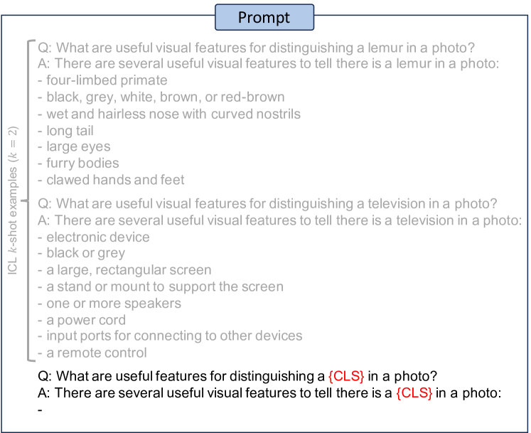
Figure 7: Prompt template applied two-shot learning for generating descriptions.

Appendix D Larger size of $N$ for Oxford Pets

Model Method $N$ RN50 RN101 ViT-B/32 ViT-B/16 CLIP (zero-shot) 0 85.4 86.2 87.0 88.9 Random 37 74.65$\pm$0.50 79.08$\pm$1.39 78.30$\pm$0.74 84.36$\pm$1.34 BADGE [2] 37 75.06$\pm$0.50 80.77$\pm$1.31 80.03$\pm$1.19 85.54$\pm$1.30 $~{}~{}+\mathrm{\texttt{PCB}}$ 37 76.51$\pm$1.83 80.94$\pm$0.42 80.22$\pm$1.69 86.22$\pm$0.71 $~{}~{}+\mathrm{\texttt{PCB}(\texttt{AE})}$ 37 76.77$\pm$0.65 83.02$\pm$0.89 81.93$\pm$0.88 87.23$\pm$0.35 $~{}~{}+\mathrm{\texttt{PCB}(\texttt{AS})}$ 37 80.09$\pm$0.85 83.48$\pm$2.13 83.16$\pm$0.18 88.10$\pm$1.49 BADGE [2] 148 86.48$\pm$0.12 89.10$\pm$0.16 88.28$\pm$0.33 91.74$\pm$0.23 $~{}~{}+\mathrm{\texttt{PCB}}$ 148 86.70$\pm$0.07 89.19$\pm$0.21 88.03$\pm$0.33 91.92$\pm$0.81 $~{}~{}+\mathrm{\texttt{PCB}(\texttt{AE})}$ 148 86.54$\pm$0.55 89.52$\pm$0.17 88.30$\pm$0.34 91.72$\pm$0.07 $~{}~{}+\mathrm{\texttt{PCB}(\texttt{AS})}$ 148 87.74$\pm$0.32 90.16$\pm$0.12 89.29$\pm$0.15 92.64$\pm$0.14 Full data - 88.0 91.1 89.3 92.7

Table 5: Ablation study as increasing query size $N$ on Oxford Pets. It shows that the small amount of training set is the crucial reason why finetuning methods underperforms zero-shot CLIP.

As shown in Table 1 and Table 2, zero-shot CLIP outperforms PCB combined with all the active learning algorithms in the case of Oxford Pets. Here, Table 5 shows that increasing query size $N$ enhances the performance. The performance when $N$ is 4 times of the number of classes (i.e. 148) surpasses the performance when $N$ is the number of classes (i.e. 37) with 4–7% points for all the architectures of an image encoder. Moreover, PCB (AS) combined with BADGE algorithm when $N$=148 almost reaches the performance when training with all the data (Full data). Through this phenomenon, setting appropriate query size $N$ is important to achieve the performance that we expect, and it should be determined by learning difficulty of the dataset.

Appendix E Additional Results

Table 2 indicates the performance on various types of architectures of an image encoder under BADGE active learning. To extend it, we conduct the experiment on various types of architectures under not only BADGE but also Entropy and Coreset active learning algorithms, and summarize the results in Table 6. Regardless of the architecture types of the image encoder, PCB combined with BADGE algorithm still has the best performance among the other baselines, but sometimes, PCB combined with Entropy algorithm beats combination of PCB and BADGE algorithm by a narrow margin. It indicates that subset $P$ sampled through the Entropy algorithm has many informative examples similar to $P$ sampled through the BADGE algorithm, where the size of $P$ is 10% of the whole dataset.

Final Accuracy ($\uparrow$) Model Method Flowers102 DTD Oxford Pets EuroSAT Caltech101 Stanford Cars Aircraft Avg Acc ($\uparrow$) RN50 CLIP (zero-shot) 65.9 41.7 85.4 41.1 82.1 55.8 19.3 55.9 Random 92.06$\pm$0.54 56.62$\pm$0.97 74.65$\pm$0.50 79.10$\pm$2.31 84.11$\pm$0.75 61.34$\pm$0.57 29.15$\pm$0.32 68.18 Entropy [16] 95.19$\pm$0.09 57.62$\pm$2.13 72.74$\pm$0.97 75.73$\pm$4.28 88.21$\pm$0.42 61.32$\pm$0.80 25.13$\pm$0.96 67.99 $~{}~{}+\mathrm{\texttt{PCB}}$ 95.30$\pm$0.59 56.44$\pm$0.39 75.49$\pm$0.45 81.69$\pm$1.63 88.78$\pm$0.43 62.02$\pm$0.17 25.75$\pm$0.35 69.35 $~{}~{}+\mathrm{\texttt{PCB}(\texttt{AE})}$ 95.75$\pm$0.23 59.02$\pm$0.59 76.59$\pm$0.12 81.77$\pm$1.51 89.41$\pm$0.53 61.05$\pm$0.99 26.44$\pm$0.81 70.00 $~{}~{}+\mathrm{\texttt{PCB}(\texttt{AS})}$ 96.17$\pm$0.27 59.34$\pm$1.09 78.59$\pm$1.41 83.26$\pm$0.35 90.49$\pm$0.02 63.52$\pm$0.31 26.46$\pm$0.99 71.12 Coreset [48] 85.02$\pm$1.51 48.74$\pm$1.00 69.87$\pm$2.36 70.02$\pm$4.16 83.34$\pm$1.33 57.93$\pm$0.56 25.38$\pm$0.62 62.90 $~{}~{}+\mathrm{\texttt{PCB}}$ 88.79$\pm$0.98 51.63$\pm$0.30 71.75$\pm$1.64 77.74$\pm$2.13 85.54$\pm$0.84 58.67$\pm$0.37 25.33$\pm$0.63 65.64 $~{}~{}+\mathrm{\texttt{PCB}(\texttt{AE})}$ 89.27$\pm$1.69 51.69$\pm$1.25 73.70$\pm$0.27 77.74$\pm$3.33 86.69$\pm$0.57 57.63$\pm$0.55 25.17$\pm$0.37 65.98 $~{}~{}+\mathrm{\texttt{PCB}(\texttt{AS})}$ 89.50$\pm$1.39 53.15$\pm$1.37 75.53$\pm$1.64 79.79$\pm$1.06 87.15$\pm$1.14 60.61$\pm$0.54 25.88$\pm$0.10 67.37 BADGE [2] 95.56$\pm$0.54 58.35$\pm$1.20 75.06$\pm$0.50 80.94$\pm$0.55 89.67$\pm$0.30 63.96$\pm$0.53 28.12$\pm$1.03 70.24 $~{}~{}+\mathrm{\texttt{PCB}}$ 95.66$\pm$0.28 57.41$\pm$0.17 76.51$\pm$1.83 80.06$\pm$0.97 89.06$\pm$0.21 63.18$\pm$0.77 29.23$\pm$0.35 70.16 $~{}~{}+\mathrm{\texttt{PCB}(\texttt{AE})}$ 95.72$\pm$0.31 59.20$\pm$1.25 76.77$\pm$0.65 81.96$\pm$0.60 89.57$\pm$0.19 62.62$\pm$0.26 28.85$\pm$1.59 70.67 $~{}~{}+\mathrm{\texttt{PCB}(\texttt{AS})}$ 96.18$\pm$0.07 59.14$\pm$1.08 80.09$\pm$0.85 81.60$\pm$2.89 90.76$\pm$0.34 66.20$\pm$0.69 29.61$\pm$0.78 71.94 Full data 97.6 71.6 88.0 93.6 92.8 78.8 42.6 80.71 RN101 CLIP (zero-shot) 65.7 43.9 86.2 33.1 85.1 62.3 19.5 56.54 Random 92.87$\pm$0.43 58.29$\pm$1.24 79.08$\pm$1.39 77.21$\pm$4.13 87.55$\pm$0.75 70.02$\pm$0.36 32.76$\pm$0.29 71.11 Entropy [16] 96.26$\pm$0.11 57.17$\pm$1.54 78.63$\pm$0.99 74.88$\pm$1.26 91.02$\pm$0.48 70.09$\pm$0.16 27.49$\pm$0.69 70.79 $~{}~{}+\mathrm{\texttt{PCB}}$ 96.26$\pm$0.25 58.81$\pm$1.39 80.14$\pm$1.27 79.91$\pm$2.06 91.62$\pm$0.30 70.87$\pm$0.45 28.11$\pm$0.38 72.25 $~{}~{}+\mathrm{\texttt{PCB}(\texttt{AE})}$ 96.47$\pm$0.39 59.81$\pm$1.34 82.65$\pm$0.99 81.23$\pm$1.26 92.16$\pm$0.90 70.14$\pm$0.56 27.96$\pm$1.63 72.92 $~{}~{}+\mathrm{\texttt{PCB}(\texttt{AS})}$ 96.49$\pm$0.17 60.70$\pm$1.09 83.64$\pm$1.02 82.43$\pm$1.35 92.86$\pm$0.20 73.62$\pm$0.67 28.68$\pm$0.83 74.06 Coreset [48] 87.90$\pm$0.92 52.23$\pm$1.76 74.02$\pm$1.81 66.62$\pm$0.54 87.23$\pm$1.18 65.83$\pm$0.43 26.37$\pm$0.42 65.74 $~{}~{}+\mathrm{\texttt{PCB}}$ 91.08$\pm$0.37 54.75$\pm$2.93 76.43$\pm$1.61 75.39$\pm$1.94 89.36$\pm$0.28 66.97$\pm$0.75 27.28$\pm$0.33 68.75 $~{}~{}+\mathrm{\texttt{PCB}(\texttt{AE})}$ 91.61$\pm$1.30 56.38$\pm$1.55 77.11$\pm$1.86 76.99$\pm$0.65 89.90$\pm$0.06 65.38$\pm$0.62 27.72$\pm$0.39 69.30 $~{}~{}+\mathrm{\texttt{PCB}(\texttt{AS})}$ 91.80$\pm$0.28 57.31$\pm$2.07 81.14$\pm$0.24 78.49$\pm$1.99 90.11$\pm$0.30 69.11$\pm$0.73 28.31$\pm$0.78 70.90 BADGE [2] 96.26$\pm$0.07 59.93$\pm$1.25 80.77$\pm$1.31 78.23$\pm$2.22 91.35$\pm$0.32 71.43$\pm$0.97 32.56$\pm$0.64 72.93 $~{}~{}+\mathrm{\texttt{PCB}}$ 95.79$\pm$0.38 60.20$\pm$1.89 80.94$\pm$0.42 79.55$\pm$1.37 91.75$\pm$0.44 71.35$\pm$0.39 32.62$\pm$1.48 73.17 $~{}~{}+\mathrm{\texttt{PCB}(\texttt{AE})}$ 96.49$\pm$0.26 62.59$\pm$0.84 83.02$\pm$0.89 81.50$\pm$0.69 92.51$\pm$0.32 71.42$\pm$0.77 32.76$\pm$0.76 74.33 $~{}~{}+\mathrm{\texttt{PCB}(\texttt{AS})}$ 96.47$\pm$0.18 62.17$\pm$1.04 83.48$\pm$2.13 81.14$\pm$1.57 92.87$\pm$0.18 74.04$\pm$0.39 32.84$\pm$0.85 75.43 Full data 97.8 74.2 91.1 92.9 94.7 83.7 46.0 82.91 ViT-B/16 CLIP (zero-shot) 70.4 46.0 88.9 54.1 88.9 65.6 27.1 63.0 Random 94.98$\pm$0.06 62.63$\pm$1.81 84.36$\pm$1.34 81.14$\pm$1.83 90.95$\pm$0.85 73.62$\pm$0.30 38.88$\pm$0.25 75.22 Entropy [16] 97.63$\pm$0.42 62.49$\pm$0.39 82.56$\pm$0.49 77.93$\pm$0.90 93.04$\pm$0.41 74.35$\pm$0.59 33.27$\pm$0.72 74.47 $~{}~{}+\mathrm{\texttt{PCB}}$ 97.75$\pm$0.08 64.93$\pm$1.02 84.89$\pm$0.59 83.48$\pm$1.37 94.23$\pm$0.23 75.68$\pm$0.26 36.03$\pm$0.43 76.71 $~{}~{}+\mathrm{\texttt{PCB}(\texttt{AE})}$ 98.06$\pm$0.35 64.36$\pm$0.47 87.08$\pm$0.90 83.55$\pm$1.95 94.56$\pm$0.34 75.15$\pm$0.55 35.60$\pm$1.58 76.91 $~{}~{}+\mathrm{\texttt{PCB}(\texttt{AS})}$ 98.48$\pm$0.14 63.81$\pm$1.24 88.03$\pm$0.60 85.92$\pm$0.85 94.89$\pm$0.28 77.58$\pm$0.43 35.84$\pm$1.71 77.79 Coreset [48] 92.12$\pm$1.45 56.07$\pm$0.90 82.17$\pm$1.82 72.17$\pm$2.72 90.66$\pm$0.45 70.12$\pm$0.83 33.28$\pm$0.45 70.94 $~{}~{}+\mathrm{\texttt{PCB}}$ 94.79$\pm$0.31 59.07$\pm$0.63 83.09$\pm$1.19 80.25$\pm$3.12 90.60$\pm$0.80 71.27$\pm$0.19 34.06$\pm$0.66 73.30 $~{}~{}+\mathrm{\texttt{PCB}(\texttt{AE})}$ 94.94$\pm$0.55 60.54$\pm$0.86 84.52$\pm$0.23 84.04$\pm$2.92 92.15$\pm$0.09 70.10$\pm$1.03 33.36$\pm$0.03 74.24 $~{}~{}+\mathrm{\texttt{PCB}(\texttt{AS})}$ 95.44$\pm$0.82 61.98$\pm$1.04 86.77$\pm$0.69 83.85$\pm$2.45 92.97$\pm$0.29 72.96$\pm$0.63 35.24$\pm$0.49 75.60 BADGE [2] 97.97$\pm$0.41 62.84$\pm$2.17 85.54$\pm$1.30 82.22$\pm$1.94 93.77$\pm$0.51 76.55$\pm$0.78 39.64$\pm$0.14 76.93 $~{}~{}+\mathrm{\texttt{PCB}}$ 98.32$\pm$0.21 64.89$\pm$1.45 86.22$\pm$0.71 81.53$\pm$3.11 93.75$\pm$0.28 76.36$\pm$0.27 40.20$\pm$0.30 77.32 $~{}~{}+\mathrm{\texttt{PCB}(\texttt{AE})}$ 98.21$\pm$0.21 65.25$\pm$1.28 87.23$\pm$0.35 84.04$\pm$2.92 94.51$\pm$0.29 75.84$\pm$0.44 39.93$\pm$0.21 77.86 $~{}~{}+\mathrm{\texttt{PCB}(\texttt{AS})}$ 98.19$\pm$0.17 64.95$\pm$1.47 88.10$\pm$1.49 83.85$\pm$2.45 95.12$\pm$0.26 78.19$\pm$0.48 40.56$\pm$0.51 78.42 Full data 99.0 77.7 92.7 95.1 95.3 85.3 53.6 85.53

Table 6: Various architectures of image encoder as an extension of Table 2. We include both all the conventional active learning algorithms and PCB combined with them in terms of various architectures of image encoder.

Appendix F Reproducibility Statement

Our intention is to make our source code publicly accessible on GitHub once it has been officially accepted. Prior to that, we privately submit for the purpose of this conference submission. For more information, please refer to the README.md file included in the compressed archive. The only excluded part in the submitted file is the dataset, as it is officially accessible and for the purpose of reducing file size.

References

- Arnab et al. [2021] Anurag Arnab, Mostafa Dehghani, Georg Heigold, Chen Sun, Mario Lučić, and Cordelia Schmid. Vivit: A video vision transformer. In Proceedings of the IEEE/CVF international conference on computer vision, pages 6836–6846, 2021.
- Ash et al. [2019] Jordan T Ash, Chicheng Zhang, Akshay Krishnamurthy, John Langford, and Alekh Agarwal. Deep batch active learning by diverse, uncertain gradient lower bounds. arXiv preprint arXiv:1906.03671, 2019.
- Beluch et al. [2018] William H Beluch, Tim Genewein, Andreas Nürnberger, and Jan M Köhler. The power of ensembles for active learning in image classification. In Proceedings of the IEEE conference on computer vision and pattern recognition, pages 9368–9377, 2018.
- Brown et al. [2020] Tom Brown, Benjamin Mann, Nick Ryder, Melanie Subbiah, Jared D Kaplan, Prafulla Dhariwal, Arvind Neelakantan, Pranav Shyam, Girish Sastry, Amanda Askell, et al. Language models are few-shot learners. Advances in neural information processing systems, 33:1877–1901, 2020.
- Cimpoi et al. [2014] Mircea Cimpoi, Subhransu Maji, Iasonas Kokkinos, Sammy Mohamed, and Andrea Vedaldi. Describing textures in the wild. In Proceedings of the IEEE conference on computer vision and pattern recognition, pages 3606–3613, 2014.
- Das et al. [2017] Abhishek Das, Satwik Kottur, Khushi Gupta, Avi Singh, Deshraj Yadav, José MF Moura, Devi Parikh, and Dhruv Batra. Visual dialog. In Proceedings of the IEEE conference on computer vision and pattern recognition, pages 326–335, 2017.
- De Vries et al. [2017] Harm De Vries, Florian Strub, Jérémie Mary, Hugo Larochelle, Olivier Pietquin, and Aaron C Courville. Modulating early visual processing by language. Advances in Neural Information Processing Systems, 30, 2017.
- Dosovitskiy et al. [2020] Alexey Dosovitskiy, Lucas Beyer, Alexander Kolesnikov, Dirk Weissenborn, Xiaohua Zhai, Thomas Unterthiner, Mostafa Dehghani, Matthias Minderer, Georg Heigold, Sylvain Gelly, et al. An image is worth 16x16 words: Transformers for image recognition at scale. arXiv preprint arXiv:2010.11929, 2020.
- Fei-Fei et al. [2004] Li Fei-Fei, Rob Fergus, and Pietro Perona. Learning generative visual models from few training examples: An incremental bayesian approach tested on 101 object categories. In 2004 conference on computer vision and pattern recognition workshop, pages 178–178. IEEE, 2004.
- Gal et al. [2017] Yarin Gal, Riashat Islam, and Zoubin Ghahramani. Deep bayesian active learning with image data. In International conference on machine learning, pages 1183–1192. PMLR, 2017.
- Gan et al. [2020] Zhe Gan, Yen-Chun Chen, Linjie Li, Chen Zhu, Yu Cheng, and Jingjing Liu. Large-scale adversarial training for vision-and-language representation learning. Advances in Neural Information Processing Systems, 33:6616–6628, 2020.
- Gao et al. [2020] Tianyu Gao, Adam Fisch, and Danqi Chen. Making pre-trained language models better few-shot learners. arXiv preprint arXiv:2012.15723, 2020.
- Geifman and El-Yaniv [2019] Yonatan Geifman and Ran El-Yaniv. Deep active learning with a neural architecture search. Advances in Neural Information Processing Systems, 32, 2019.
- He et al. [2016] Kaiming He, Xiangyu Zhang, Shaoqing Ren, and Jian Sun. Deep residual learning for image recognition. In Proceedings of the IEEE conference on computer vision and pattern recognition, pages 770–778, 2016.
- Helber et al. [2019] Patrick Helber, Benjamin Bischke, Andreas Dengel, and Damian Borth. Eurosat: A novel dataset and deep learning benchmark for land use and land cover classification. IEEE Journal of Selected Topics in Applied Earth Observations and Remote Sensing, 12(7):2217–2226, 2019.
- Holub et al. [2008] Alex Holub, Pietro Perona, and Michael C Burl. Entropy-based active learning for object recognition. In 2008 IEEE Computer Society Conference on Computer Vision and Pattern Recognition Workshops, pages 1–8. IEEE, 2008.
- Houlsby et al. [2011] Neil Houlsby, Ferenc Huszár, Zoubin Ghahramani, and Máté Lengyel. Bayesian active learning for classification and preference learning. arXiv preprint arXiv:1112.5745, 2011.
- Jia et al. [2021] Chao Jia, Yinfei Yang, Ye Xia, Yi-Ting Chen, Zarana Parekh, Hieu Pham, Quoc Le, Yun-Hsuan Sung, Zhen Li, and Tom Duerig. Scaling up visual and vision-language representation learning with noisy text supervision. In International conference on machine learning, pages 4904–4916. PMLR, 2021.
- Jiang et al. [2020] Zhengbao Jiang, Frank F Xu, Jun Araki, and Graham Neubig. How can we know what language models know? Transactions of the Association for Computational Linguistics, 8:423–438, 2020.
- Ju et al. [2022] Chen Ju, Tengda Han, Kunhao Zheng, Ya Zhang, and Weidi Xie. Prompting visual-language models for efficient video understanding. In European Conference on Computer Vision, pages 105–124. Springer, 2022.
- Khattak et al. [2023a] Muhammad Uzair Khattak, Hanoona Rasheed, Muhammad Maaz, Salman Khan, and Fahad Shahbaz Khan. Maple: Multi-modal prompt learning. In Proceedings of the IEEE/CVF Conference on Computer Vision and Pattern Recognition, pages 19113–19122, 2023a.
- Khattak et al. [2023b] Muhammad Uzair Khattak, Syed Talal Wasim, Muzammal Naseer, Salman Khan, Ming-Hsuan Yang, and Fahad Shahbaz Khan. Self-regulating prompts: Foundational model adaptation without forgetting. In Proceedings of the IEEE/CVF International Conference on Computer Vision, pages 15190–15200, 2023b.
- Kirsch et al. [2019] Andreas Kirsch, Joost Van Amersfoort, and Yarin Gal. Batchbald: Efficient and diverse batch acquisition for deep bayesian active learning. Advances in neural information processing systems, 32, 2019.
- Körner and Wrobel [2006] Christine Körner and Stefan Wrobel. Multi-class ensemble-based active learning. In European conference on machine learning, pages 687–694. Springer, 2006.
- Krause et al. [2013] Jonathan Krause, Michael Stark, Jia Deng, and Li Fei-Fei. 3d object representations for fine-grained categorization. In Proceedings of the IEEE international conference on computer vision workshops, pages 554–561, 2013.
- Lester et al. [2021] Brian Lester, Rami Al-Rfou, and Noah Constant. The power of scale for parameter-efficient prompt tuning. arXiv preprint arXiv:2104.08691, 2021.
- Lewis and Catlett [1994] David D Lewis and Jason Catlett. Heterogeneous uncertainty sampling for supervised learning. In Machine learning proceedings 1994, pages 148–156. Elsevier, 1994.
- Li et al. [2020] Gen Li, Nan Duan, Yuejian Fang, Ming Gong, and Daxin Jiang. Unicoder-vl: A universal encoder for vision and language by cross-modal pre-training. In Proceedings of the AAAI conference on artificial intelligence, pages 11336–11344, 2020.
- Li et al. [2021] Junnan Li, Ramprasaath Selvaraju, Akhilesh Gotmare, Shafiq Joty, Caiming Xiong, and Steven Chu Hong Hoi. Align before fuse: Vision and language representation learning with momentum distillation. Advances in neural information processing systems, 34:9694–9705, 2021.
- Li et al. [2022] Junnan Li, Dongxu Li, Caiming Xiong, and Steven Hoi. Blip: Bootstrapping language-image pre-training for unified vision-language understanding and generation. In International Conference on Machine Learning, pages 12888–12900. PMLR, 2022.
- Li et al. [2023] Junnan Li, Dongxu Li, Silvio Savarese, and Steven Hoi. Blip-2: Bootstrapping language-image pre-training with frozen image encoders and large language models. arXiv preprint arXiv:2301.12597, 2023.
- Li and Liang [2021] Xiang Lisa Li and Percy Liang. Prefix-tuning: Optimizing continuous prompts for generation. arXiv preprint arXiv:2101.00190, 2021.
- Lu et al. [2019] Jiasen Lu, Dhruv Batra, Devi Parikh, and Stefan Lee. Vilbert: Pretraining task-agnostic visiolinguistic representations for vision-and-language tasks. Advances in neural information processing systems, 32, 2019.
- Lu et al. [2022] Yuning Lu, Jianzhuang Liu, Yonggang Zhang, Yajing Liu, and Xinmei Tian. Prompt distribution learning. In Proceedings of the IEEE/CVF Conference on Computer Vision and Pattern Recognition, pages 5206–5215, 2022.
- Maji et al. [2013] Subhransu Maji, Esa Rahtu, Juho Kannala, Matthew Blaschko, and Andrea Vedaldi. Fine-grained visual classification of aircraft. arXiv preprint arXiv:1306.5151, 2013.
- Melville and Mooney [2004] Prem Melville and Raymond J Mooney. Diverse ensembles for active learning. In Proceedings of the twenty-first international conference on Machine learning, page 74, 2004.
- Menon and Vondrick [2023] Sachit Menon and Carl Vondrick. Visual classification via description from large language models. In The Eleventh International Conference on Learning Representations, 2023.
- Munjal et al. [2022] Prateek Munjal, Nasir Hayat, Munawar Hayat, Jamshid Sourati, and Shadab Khan. Towards robust and reproducible active learning using neural networks. In Proceedings of the IEEE/CVF Conference on Computer Vision and Pattern Recognition, pages 223–232, 2022.
- Nilsback and Zisserman [2008] Maria-Elena Nilsback and Andrew Zisserman. Automated flower classification over a large number of classes. In 2008 Sixth Indian conference on computer vision, graphics & image processing, pages 722–729. IEEE, 2008.
- Parkhi et al. [2012] Omkar M Parkhi, Andrea Vedaldi, Andrew Zisserman, and CV Jawahar. Cats and dogs. In 2012 IEEE conference on computer vision and pattern recognition, pages 3498–3505. IEEE, 2012.
- Parvaneh et al. [2022] Amin Parvaneh, Ehsan Abbasnejad, Damien Teney, Gholamreza Reza Haffari, Anton Van Den Hengel, and Javen Qinfeng Shi. Active learning by feature mixing. In Proceedings of the IEEE/CVF Conference on Computer Vision and Pattern Recognition, pages 12237–12246, 2022.
- Pratt et al. [2023] Sarah Pratt, Ian Covert, Rosanne Liu, and Ali Farhadi. What does a platypus look like? generating customized prompts for zero-shot image classification. In Proceedings of the IEEE/CVF International Conference on Computer Vision, pages 15691–15701, 2023.
- Qi et al. [2020] Di Qi, Lin Su, Jia Song, Edward Cui, Taroon Bharti, and Arun Sacheti. Imagebert: Cross-modal pre-training with large-scale weak-supervised image-text data. arXiv preprint arXiv:2001.07966, 2020.
- Radford et al. [2021] Alec Radford, Jong Wook Kim, Chris Hallacy, Aditya Ramesh, Gabriel Goh, Sandhini Agarwal, Girish Sastry, Amanda Askell, Pamela Mishkin, Jack Clark, et al. Learning transferable visual models from natural language supervision. In International conference on machine learning, pages 8748–8763. PMLR, 2021.
- Rakesh and Jain [2021] Vineeth Rakesh and Swayambhoo Jain. Efficacy of bayesian neural networks in active learning. In Proceedings of the IEEE/CVF Conference on Computer Vision and Pattern Recognition, pages 2601–2609, 2021.
- Ren et al. [2021] Pengzhen Ren, Yun Xiao, Xiaojun Chang, Po-Yao Huang, Zhihui Li, Brij B Gupta, Xiaojiang Chen, and Xin Wang. A survey of deep active learning. ACM computing surveys (CSUR), 54(9):1–40, 2021.
- Roth and Small [2006] Dan Roth and Kevin Small. Margin-based active learning for structured output spaces. In Machine Learning: ECML 2006: 17th European Conference on Machine Learning Berlin, Germany, September 18-22, 2006 Proceedings 17, pages 413–424. Springer, 2006.
- Sener and Savarese [2018] Ozan Sener and Silvio Savarese. Active learning for convolutional neural networks: A core-set approach. In International Conference on Learning Representations, 2018.
- Settles [2009] Burr Settles. Active learning literature survey. 2009.
- Shin et al. [2020] Taylor Shin, Yasaman Razeghi, Robert L Logan IV, Eric Wallace, and Sameer Singh. Autoprompt: Eliciting knowledge from language models with automatically generated prompts. arXiv preprint arXiv:2010.15980, 2020.
- Touvron et al. [2023a] Hugo Touvron, Thibaut Lavril, Gautier Izacard, Xavier Martinet, Marie-Anne Lachaux, Timothée Lacroix, Baptiste Rozière, Naman Goyal, Eric Hambro, Faisal Azhar, et al. Llama: Open and efficient foundation language models. arXiv preprint arXiv:2302.13971, 2023a.
- Touvron et al. [2023b] Hugo Touvron, Louis Martin, Kevin Stone, Peter Albert, Amjad Almahairi, Yasmine Babaei, Nikolay Bashlykov, Soumya Batra, Prajjwal Bhargava, Shruti Bhosale, et al. Llama 2: Open foundation and fine-tuned chat models. arXiv preprint arXiv:2307.09288, 2023b.
- Vaswani et al. [2017] Ashish Vaswani, Noam Shazeer, Niki Parmar, Jakob Uszkoreit, Llion Jones, Aidan N Gomez, Lukasz Kaiser, and Illia Polosukhin. Attention is all you need. Advances in neural information processing systems, 30, 2017.
- Yang et al. [2022] Jingfeng Yang, Aditya Gupta, Shyam Upadhyay, Luheng He, Rahul Goel, and Shachi Paul. Tableformer: Robust transformer modeling for table-text encoding. arXiv preprint arXiv:2203.00274, 2022.
- Yao et al. [2021] Lewei Yao, Runhui Huang, Lu Hou, Guansong Lu, Minzhe Niu, Hang Xu, Xiaodan Liang, Zhenguo Li, Xin Jiang, and Chunjing Xu. Filip: Fine-grained interactive language-image pre-training. arXiv preprint arXiv:2111.07783, 2021.
- Yu et al. [2021] Fei Yu, Jiji Tang, Weichong Yin, Yu Sun, Hao Tian, Hua Wu, and Haifeng Wang. Ernie-vil: Knowledge enhanced vision-language representations through scene graphs. In Proceedings of the AAAI Conference on Artificial Intelligence, pages 3208–3216, 2021.
- Yu et al. [2023] Tao Yu, Zhihe Lu, Xin Jin, Zhibo Chen, and Xinchao Wang. Task residual for tuning vision-language models. In Proceedings of the IEEE/CVF Conference on Computer Vision and Pattern Recognition, pages 10899–10909, 2023.
- Yuan et al. [2021] Lu Yuan, Dongdong Chen, Yi-Ling Chen, Noel Codella, Xiyang Dai, Jianfeng Gao, Houdong Hu, Xuedong Huang, Boxin Li, Chunyuan Li, et al. Florence: A new foundation model for computer vision. arXiv preprint arXiv:2111.11432, 2021.
- Yun et al. [2019] Seongjun Yun, Minbyul Jeong, Raehyun Kim, Jaewoo Kang, and Hyunwoo J Kim. Graph transformer networks. Advances in neural information processing systems, 32, 2019.
- Zhai et al. [2022] Xiaohua Zhai, Xiao Wang, Basil Mustafa, Andreas Steiner, Daniel Keysers, Alexander Kolesnikov, and Lucas Beyer. Lit: Zero-shot transfer with locked-image text tuning. In Proceedings of the IEEE/CVF Conference on Computer Vision and Pattern Recognition, pages 18123–18133, 2022.
- Zhong et al. [2021] Zexuan Zhong, Dan Friedman, and Danqi Chen. Factual probing is [mask]: Learning vs. learning to recall. arXiv preprint arXiv:2104.05240, 2021.
- Zhou et al. [2022a] Kaiyang Zhou, Jingkang Yang, Chen Change Loy, and Ziwei Liu. Conditional prompt learning for vision-language models. In Proceedings of the IEEE/CVF Conference on Computer Vision and Pattern Recognition, pages 16816–16825, 2022a.
- Zhou et al. [2022b] Kaiyang Zhou, Jingkang Yang, Chen Change Loy, and Ziwei Liu. Learning to prompt for vision-language models. International Journal of Computer Vision, 130(9):2337–2348, 2022b.