Total positivity and spectral theory for Toeplitz Hessenberg matrix ensembles

Abstract

In this paper we define and lay the groundwork for studying a novel matrix ensemble: totally positive Hessenberg Toeplitz operators, denoted TPHT. This is the intersection of two ensembles that have been significantly explored: totally positive Hessenberg matrices (TPH) and Hessenberg Toeplitz matrices (HT). TPHT has a rich linear algebraic and spectral structure that we describe. Along the way we find some previously unnoticed connections between certain Toeplitz normal forms for matrices and Lie theoretic interpretations. We also numerically study the spectral asymptotics of TPH matrices via the TPHT ensemble and use this to open a study of TPHT with random symbols.

15B05, 15B48, 15B52, 47B35, 60B15, 60B20

1 Introduction

This paper concerns a particular subclass of Hessenberg matrices and their spectral asymptotics. The $n\times n$ (lower) Hessenberg matrices, $\mathcal{H}$, in general take the form

$$\left(\begin{array}[]{ccccc}*&1&&&\\ &*&1&&\\ \vdots&\ddots&\ddots&\ddots&\\ \vdots&&\ddots&\ddots&1\\ &\dots&\dots&*&*\end{array}\right).$$

The first subclass we consider is the totally positive Hessenberg matrices (TPH). We follow a standard convention here by taking totally positive (TP) to mean that all minors are non-negative. (If we mean to say that all minors are positive we will refer to this as being strictly TP.) This enables us to characterize other sparsity patterns as being TP, such as lower triangular TP matrices.

Hessenberg matrices themselves have played an elemental role in many areas of linear and numerical linear algebra. For instance, every matrix is conjugate via a Householder reflector to a Hessenberg matrix, called its Hessenberg form. The Hessenberg form is preserved by the QR decomposition, and so is an essential component of many tools used to compute eigenvalues and eigenvectors, including the QR algorithm, Lanczos Iterations, and generalized minimal residual method (GMRES) [16, 17, 25, 26, 32]. Additionally, Hessenberg matrices are essential in Neville elimination, an alternative to Gaussian elimination to find an LU decomposition that iteratively zeros out each subdiagonal and so maintains an upper Hessenberg form that moves toward the final upper triangular factor [19].

More recently there has been a particular focus on the TPH ensembles we consider here. These bring to bear tools from other areas of mathematics such as network theory and dynamical systems theory. TPH ensembles have played a fundamental role in studying the analytical combinatorics of networks because they are generalizations of path-counting matrices [15]. Consequently, this class of matrices has natural coordinatizations stemming from Whitney-Loewner factorization (see Theorem 2.6). That in turn has applications to the dynamics of LU factorizations as well as to integrable Toda lattices and their generalizations. In particular this makes a connection to recent work on integrable systems theory and analytical combinatorics. In [14], we find simultaneous TPH realizations of the integrable Full Toda lattice [12] on different space-time scales. For discrete space-time we realize a novel combinatorial interpretation of the LU algorithm in terms of the dynamics of extended box-ball systems. In related work [18] Fukuda and others have made use of Full Toda lattices and formal connections to orthogonal polynomials to try to develop improved eigenvalue algorithms for totally positive Hessenberg (TPH) matrices. This appears to have potential connections to the rigorous analysis of bi-orthogonal polynomials developed in [13]. Other applications, by Demmel and Koev, concern high relative accuracy for eigenvalue calculations (see [7, 23]).

In another direction there has been a recent focus on a different class of matrices that is both Hessenberg and Toeplitz (HT) with many applications in linear algebra related for example to orthogonal polynomials, stochastic filters, time series analysis and difference approximations to initial-BVP problems for PDE [22].

In this paper we begin to analyze questions that lie naturally at the intersection of these two classes: totally positive Hessenberg Toeplitz matrices (TPHT). The key point for our work here is that each isospectral class of Hessenberg matrices contains a unique Toeplitz matrix. This allows us to bring forward and apply powerful tools from Toeplitz theory to investigate spectral questions for general TPH matrices. This ties into another more recent and principal motivation for this work which concerns the study of integrable systems evolving on spaces of random or rough data. That work seeks to gain insights into dynamics of more general conservative evolution equations in random environments (see [33] for a general survey). Past models have focused on the classical Toda whose phase space is tridiagonal Hessenberg matrices with independent random entries. The recent work in [14] suggests how these studies may be extended to general TPH ensembles with appropriate random entries. These motivations will be further described in Section 4, but our overall goal here is to take a step toward showing that such studies may be reduced to considering spectra of random TPHT class. Along the way we uncover some novel aspects of the linear algebra underlying this class.

The outline of this paper is as follows. In Section 2 we present the essential background for the two fundamental classes, HT and TPH, on which this work is based. In particular we review some of the relevant remarkable properties of TP matrices and illustrate their realization within the TPH ensemble. We then introduce the novel aspects of the intersection ensemble, TPHT, of TPH and HT. Along the way we describe results on HT normal forms for general Hessenberg matrices. We show that these normal forms are very naturally related to more general normal forms in Lie theory originally due to Kostant. We believe this is the first time this connection has been noticed and we make use of it in later sections as well as relating it to other natural normal forms (detailed in the Appendix). Finally we discuss connections of the HT normal form to LU factorization, providing also the explicit LU form for TPHT matrices in Theorem 2.9.

In Section 3 we review the Grenander-Szegő theory that provides the principal tool for understanding spectral asymptotics within TPH.

Section 4 motivates our numerical study of the spectral theory of TPH and how to access this through TPHT. The bulk of the section presents random realizations of the spectral asymptotics.

In Section 5, we describe a number of potential applications for our work. Finally, in Appendix A we detail the aforementioned interplay between various normal forms for the TPHT ensemble while Appendix B contains the detailed proof for Theorem 2.9.

2 Background and Motivation

2.1 Hessenberg-Toeplitz Normal Form

Toeplitz matrices are distinguished by having constant values along diagonals. More precisely, an $n\times n$ matrix $X$ is Toeplitz if there are $2n-1$ numbers, $x_{-n+1},\dots,x_{0},\dots,x_{n-1}$ such that the $(i,j)$ coefficient of $X$ is $x_{j-i}$ for $1\leq i,j\leq n$.

Mackey, Mackey and Petrovic derived the following elegant, constructive result in [27]. First recall that a nonderogatory matrix is defined as one all of whose eigenspaces are one-dimensional, meaning that each eigenvalue corresponds to one and only one Jordan block. Also let $M_{n}(\mathbb{R})$ denote the space of of $n\times n$ matrices over $\mathbb{R}$.

Theorem 2.1 ([27]).

Every nonderogatory element of $M_{n}(\mathbb{R})$ is similar to a unique Hessenberg-Toeplitz (HT) matrix. Alternatively, every nonderogatory isospectral class contains a unique HT matrix.

Since elements of the space of $n\times n$ Hessenberg matrices, denoted $\mathcal{H}_{n}$, are all nonderogatory (see Proposition 1f of [27]), one has the following:

Corollary 2.2.

Every isospectral class in $\mathcal{H}_{n}$ with respective (possibly repeated) eigenvalues $\Lambda=\{\lambda_{1},\dots\lambda_{n}\}$, and denoted $\mathcal{O}_{\Lambda}$, contains a unique Toeplitz matrix.

Remark 2.3.

This explicit result is an instance of a more general, but not constructive, Lie theoretic result due to Kostant [24]. In essence, this states that for the analogue of Hessenberg matrices in a semi-simple Lie algebra, there is a cross-section of the isospectral classes such that elements of a given isospectral class are conjugate to a unique element of the cross-section with the conjugation given by a unique lower unipotent matrix. In our case that cross-section is given by Toeplitz matrices. This is more precisely stated in Appendices A and B where other, constructive, normal forms of potential interest to us are also presented.

These results and their applications provide a strong motivation for our study of the HT class. The focus of this paper is to study aspects of a class with the further restriction of being totally positive, the TPHT class.

For later use we introduce here the notion of the symbol of a Toeplitz operator, $T$, which is the Taylor-Laurent series (or Fourier series) whose $k^{th}$ coefficient is taken to be the constant value along the $k^{th}$ diagonal of a bi-infinite Toeplitz matrix. In the application for this paper we will be concerned with symbols that correspond to polynomials of Hessenberg type, meaning of the form $\varphi(T)=t^{-1}(1+x_{1}t+\dots+x_{n}t^{n})$ (or trigonometric polynomials in the Fourier presentation). Toeplitz matrices are then formed by taking finite size truncations of the associated bi-infinite matrix. For more on the characterization of Toeplitz operators in the bi-infinite setting we refer the reader to the seminal paper of Aissen, Edrei, Schoenberg and Whitney [1]. See also remarks in the Conclusions.

2.2 Totally Positive Hessenberg matrices

TP matrices themselves have a rich structure, which is nicely described in Ando’s survey [2]. One of the most salient of these are spectral oscillation properties that generalize classical Perron-Frobenius results for positive matrices. More precisely one has

Theorem 2.4 ([2]).

If $A$ is an $n\times n$ strictly TP matrix then all its eigenvalues are real, distinct and positive. Let $\mathbf{u}_{k}$ denote the (real) eigenvector corresponding to the $k^{th}$ eigenvalue (in descending ordered), then $\mathbf{u}_{k}$ has exactly $k-1$ variations of sign. Moreover, the nodes of ${u}_{k}(t)$ and those of ${u}_{k+1}(t)$ are interlacing.

By a variation of sign here we mean consecutive entries in the eigenvector where the sign changes. For ${u}_{k}(t)$ we have the following general definition. For a vector $\mathbf{x}\in\mathbb{R}^{n}$ define the piece-wise linear function $x(t)$ for $1\leq t\leq n$ by

$$x(t)=(k+1-t)x_{k}+(t-k)x_{k+1}\quad\mbox{for}\,\,\,k\leq t\leq k+1.$$

The nodes of $x(t)$ are the roots of $x(t)=0$.

If $A$ is TP but not strictly so, then it is in the closure of strictly TP matrices (see Theorem 2.7 of [2]). In particular, if $A$ has full rank with distinct eigenvalues (which will be the case for the Hessenberg matrices we will consider) then the stated results of the theorem continue to hold but with the possibility that some zero crossings might coalesce at an intermediate node.

Definition 2.5.

We will denote the cases of $n\times n$ Toeplitz matrices with (factored) symbol $\varphi(T)=t^{-1}\prod_{j=1}^{m}(1+a_{j}t)^{m}$ by $({\textbf{a}_{m}},n)$. Let $\textbf{1}_{m}$ denote the vector in $\mathbb{R}^{m}$ whose components are all $1$. When $m=n$ we just write ${\textbf{a}_{n}}$ or $\textbf{1}_{n}$ for the associated Toeplitz matrix.

We illustrate all this in the following examples along with Figure 1 for the case of Toeplitz matrices with symbols $t^{-1}(1+t)^{5}$ and $t^{-1}(1+t)^{10}$, where we display the relevant information in two panels for $\textbf{1}_{5}$ and $\textbf{1}_{10}$, respectively. In the first case (3) shows the eigenvalues ordered by decreasing size. Then (4) displays the matrix of the associated eigenvectors in corresponding order. Finally Figure 1a shows the piece-wise linear interpolations of the eigenvectors, oriented vertically to the correspondence with the eigenvectors in (4). Bars are included in this figure to mark where the zero-crossings occur. A similar set of panels is shown for $\textbf{1}_{10}$ culminating in Figure 1b.

For the case of symbol $t^{-1}(1+t)^{5}$, whose coefficients would then align with the standard binomial coefficients, the matrix truncated to size $5$ is as follows.

(2) $$\textbf{1}_{5} =\begin{bmatrix}5&1&0&0&0\\ 10&5&1&0&0\\ 10&10&5&1&0\\ 5&10&10&5&1\\ 1&5&10&10&5\end{bmatrix}=V\Lambda V^{-1},$$

where $\Lambda$ and $V$ denote, respectively, the eigenvalue and eigenvector matrices, with approximate computed forms of

(3) $$\Lambda \approx\operatorname{diag}(11.0024,7.9317,4.3187,1.5285,0.2187),$$

(4) $$V \approx\begin{bmatrix}0.0047&-0.0065&0.0105&-0.0182&-0.0258\\ 0.0283&-0.0190&-0.0071&0.0632&0.1234\\ 0.1226&0.0091&-0.0999&-0.0373&-0.3319\\ 0.4061&0.2822&0.0347&-0.3203&0.6111\\ 0.9051&0.9591&0.9943&0.9443&-0.7075\end{bmatrix}$$

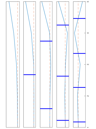
(a) $\textbf{1}_{5}$

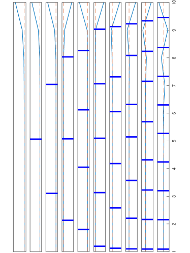
(b) $\textbf{1}_{10}$

Figure 1: Oscillating eigenvector interlacing zero maps for $n\times n$ matrix $\textbf{1}_{n}$, formed using $n=5,10$, ordered in decreasing associated eigenvalue size, with dotted red line indicating the standard $x$-axis and blue bars indicating associated zero crossings.

One may directly check that (2) is TP. To further illustrate the TP properties of the eigenvalues and eigenvectors of (2), we have that the (computed) eigenvalues are strictly positive while the associated (computed) eigenvector matrix illustrates the sign variation property of the theorem. In summary, the oscillatory properties we exemplify in this example include:

1. Perron-Frobenius theorem: There is an eigenvector for the largest eigenvalue with positive components. This is clearly seen in the leftmost displays of and Figures 1a and 1b as well as by the first column of (4).

2. Each successive eigenvector (with respect to the ordering of the eigenvalues from largest to smallest) introduces an additional sign change from the prior step. For instance in (4) one sees that the entries in the leftmost eigenvector are all positive; in the next eigenvector there is one sign change between the second and third entry; in the third eigenvector there are two sign changes, one between the first and second entries and another between the third and fourth entries; and so on. This is the variation of signs stated in the theorem.

3. The piecewise linear maps that connect the points $(j,v_{k,j})$ for successive eigenvectors $\mathbf{v}_{k}$ have interlacing zeros (nodes of the $v_{k}(t)$ described in the theorem.) This interlacing is clear from the interlacing of the consecutive bar configurations in Figures 1a and 1b.

It is natural to seek a characterization of TPH matrices along the lines of what was described for Toeplitz matrices. A step in that direction was carried out in [14], which approaches this in terms of LU factorization. This essentially follows from the Whitney-Loewner theorem [15] . The result is

Theorem 2.6 ([14]).

Let $\mathcal{B}$ denote the subvariety of $\mathcal{H}_{n}$ comprised of upper bidiagonal matrices of the form

$$\left[\begin{array}[]{cccc}*&1\\ &*&\ddots\\ &&\ddots&1\\ &&&*\end{array}\right]$$

and let $\mathcal{B}^{\geq 0}$ denote the submanifold in which all diagonal entries are positive. Then the subvariety, TPH, of totally positive Hessenberg matrices has the decomposition

(6) $$\mathcal{H}^{\geq 0}=(N_{-}^{\geq 0}\times\mathcal{B}^{\geq 0}~{})$$

where the superscript, $\{\geq 0\}$, denotes total positivity. ($N_{-}$ here denotes the space of $n\times n$ lower unipotent matrices.)

As is further discussed in [14], the LU decomposition described in the theorem can be iterated to define a dynamic process on $\mathcal{H}_{n}$. This is an isospectral process that can be used to approximate eigenvalues by iteratively computing the $A=A^{(0)}=LU$ factorization of an input matrix and then inverting the order of the factors for $A^{(1)}=UL=UA^{(0)}U^{-1}$; this is followed by iteratively computing the LU factorization of $A^{(i+1)}$ from input $A^{(i)}$. TP matrices have the additional property that each LU factor is itself TP while also the product of TP matrices is TP [2, 6]. So each intermediate matrix in the iterated LU algorithm is TP. Since the process is isospectral, the eigenvalues never change. The eigenvectors do change; however, they maintain the oscillatory properties, stated in Theorem 2.4, throughout. For example, Figures 2a and 2b show the oscillating eigenvector interlacing zero maps for the 10^th iterate of the LU map (denoted $\textbf{1}_{n}^{(10)}$) using $\textbf{1}_{n}$ for $n=5,10$ (cf. Figures 1a and 1b). In Appendix A an explicit expression for the eigenvectors is given in terms of normal forms (see Corollary A.10).

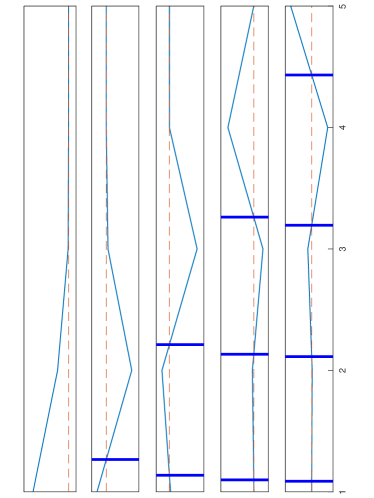
(a) $\textbf{1}_{5}^{(10)}$

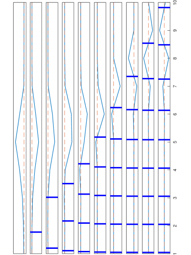
(b) $\textbf{1}_{10}^{(10)}$

Figure 2: Oscillating eigenvector interlacing zero maps for $n\times n$ matrix $\textbf{1}_{n}^{(10)}$, formed using $n=5,10$.

2.3 The Hessenberg-Toeplitz Normal form and Total Positivity

TPH matrices are, of course, a subclass of the general class of Hessenberg matrices and in particular they form a subclass within each isospectral class, $\mathcal{O}_{\Lambda}$, of Hessenberg matrices with fixed spectrum $\Lambda$. This raises the natural question of whether the unique Toeplitz matrix of Corollary 2.2 is TP, i.e. an element of TPHT. (Of course in these TP cases one should restrict attention to $\Lambda$ with all eigenvalues non-negative.)

The Hessenberg Toeplitz (HT) operators we consider are finite banded with symbols, as defined in Section 2.1, of the (factored) form

(7) $$\varphi(T)(z)=z^{-1}\prod_{\ell=1}^{n}(1+a_{\ell}z).$$

We note that this HT symbol amounts to an upward shift of the diagonals for operators corresponding to symbols that are polynomial and, therefore, whose associated bi-infinite matrix operator is lower triangular. Since the $a_{\ell}$ are non-negative in the TPHT case, it then follows (see Theorem 5.1) that the corresponding $n\times n$ truncations, $T_{n}$, of these TPHT operators have non-negative minors and so are TP. Hence, the $n\times n$ TPHT matrices depend on $n$ real, non-negative parameters, the $a_{\ell}$.

We then have the following key result.

Corollary 2.7.

TPHT is the closure of an open set within the class of HT matrices and therefore represents the closure of an open set of isospectral equivalence classes in $\mathcal{H}_{n}$.

The first statement follows because the class of HT $n\times n$ matrices is $n$-dimensional, as is TPHT. The rest of the statement follows from Corollary 2.2. By Kostant’s theorem (cf. Appendix A) the isospectral classes in $\mathcal{H}_{n}$ are conjugacy classes under the adjoint action of $N_{-}$ on $\mathcal{H}_{n}$. Hence, by Corollary 2.2, we have a 1:1 correspondence

$$\mathcal{H}_{n}/N_{-} \to HT$$

$$\mathcal{O}_{\Lambda} \mapsto T_{\Lambda}$$

defined by mapping the isospectral class to the unique HT matrix it contains, denoted by $T_{\Lambda}$. Since, by Corollary 2.2 this is 1:1 and TPHT is the closure of an open subset of HT, the latter statement of Corollary 2.7 follows.

So TPHT is a robust and natural class to study.

2.4 LU Factorization in the HT Ensemble

We pause here to discuss how one may identify the unique HT operator within a given isospectral class of $\mathcal{H}_{n}$. For this we can make use of the LU decomposition described in Theorem 2.6.

For convenience of notation, in the following definition and theorem, if $n\in\mathbb{N}$, denote by $[n]$ the set $\{1,2,\ldots,n\}$. If $n<1$, we shall take $[n]$ to be the empty set.

Definition 2.8.

Let $A$ be an $n\times n$ matrix and $S\subseteq\{1,2,\ldots,n\}$. If $S$ is non-empty, denote by $\tau_{S}^{\text{init}}(A)$ the minor for the associated sub-matrix of $A$ with columns given by the initial $|S|$ columns of $A$ and rows indexed by $S$:

$$\tau_{S}^{\text{init}}(A)=\det\left(A_{S,[|S|]}\right).$$

If $S$ is the empty set, we take this to be $1$.

Theorem 2.9.

Let $T$ be an $n\times n$ TPHT matrix in $\mathcal{H}^{\geq 0}$, defined in Theorem 2.6. Then $T$ has the LU decomposition $T=LU$ where

$$(L)_{ij} =\left\{\begin{array}[]{cc}0&i<j\\ \frac{\tau_{\{i\}\cup[j-1]}^{\text{init}}(T)}{\tau_{[j]}^{\text{init}}(T)}&i\geq j\end{array}\right.$$

$$(U)_{ij} =\left\{\begin{array}[]{cc}\frac{\tau_{[i]}^{\text{init}}(T)}{\tau_{[i-1]}^{\text{init}}(T)}&i=j\\ 1&j=i+1\\ 0&\text{otherwise.}\end{array}\right.$$

Proof 2.10 (Sketch of proof:).

We provide here just a sketch of the full proof which can be found in Appendix B. The key property used is the explicit form of LU decompositions in the class of Hessenberg matrices. Take the LU decomposition of an $(n+1)\times(n+1)$ Hessenberg matrix:

$$\left[\begin{array}[]{c|c}L_{n+1}^{(n)}&\mathbf{0}_{n}\\ \hline\cr\mathbf{p}^{T}&1\end{array}\right]\left[\begin{array}[]{c|c}U_{n+1}^{(n)}&\mathbf{q}\\ \hline\cr\mathbf{0}_{n}^{T}&r\end{array}\right]=\left[\begin{array}[]{c|c}L_{n+1}^{(n)}U_{n+1}^{(n)}&L_{n+1}^{(n)}\mathbf{q}\\ \hline\cr\mathbf{p}^{T}U_{n+1}^{(n)}&\mathbf{p}^{T}\mathbf{q}+r\end{array}\right],$$

where $L_{n+1}^{(n)}$ and $U_{n+1}^{(n)}$ are both $n\times n$. This then says that respective principal submatrices of the lower and upper matrices of a Hessenberg matrix then themselves constitute an LU decomposition of the corresponding principal submatrix of the Hessenberg matrix.
The proof we provide leverages this fact to prove Theorem 2.9 inductively, with the induction step amounting to solving for the unknowns $\mathbf{p}$, $\mathbf{q}$ and $r$. Solving for these unknowns and recognizing the resulting conditions for Theorem 2.9 to be true as cofactor expansions allows the proof to be completed.

In [14] an alternative parameterization of TPH matrices, due to Lusztig, is employed. This is given in terms of a further factorization of $L$ of the form

(8) $$L=(1+\alpha_{1}f_{h_{1}})\cdots(1+\alpha_{M}f_{h_{M}})$$

where $L\in N^{\geq 0}_{-}$, $M=\binom{n}{2}$, $h_{j}\in\{1,\dots,n\}$, $\alpha_{j}\in\mathbb{R}_{>0}$, 1 denotes the identity matrix and $f_{i}$ is the elementary lower matrix with 1 in the $(i+1,i)$ entry and zero elsewhere. The choice and ordering of the $h_{i}$ is determined by a rule described in [14]. In this way an element of TPH, with given eigenvalues, may be uniquely decomposed into a product of bidiagonal matrices. Thus the $\alpha_{j}$ provide an alternative parameterization of TPH. We will not make much mention of this parameterization in the present paper but illustrate here what this decomposition looks like in the case of a $3\times 3$ TPHT matrix, in terms of the coefficient parameters of the Toeplitz symbol.

Let $T$ be the following TPHT matrix

(12) $$T=\left[\begin{array}[]{ccc}a_{1}&1&0\\ a_{2}&a_{1}&1\\ a_{3}&a_{2}&a_{1}\end{array}\right].$$

First, decompose $T$ using Theorem 2.9:

(22) $$T=\left[\begin{array}[]{ccc}a_{1}&1&0\\ a_{2}&a_{1}&1\\ a_{3}&a_{2}&a_{1}\end{array}\right]=\left[\begin{array}[]{ccc}1&0&0\\ \frac{a_{2}}{a_{1}}&1&0\\ \frac{a_{3}}{a_{1}}&\frac{a_{1}a_{2}-a_{3}}{a_{1}^{2}-a_{2}}&1\end{array}\right]\left[\begin{array}[]{ccc}a_{1}&1&0\\ 0&\frac{a_{1}^{2}-a_{2}}{a_{1}}&1\\ 0&0&\frac{a_{1}^{3}-2a_{1}a_{2}-a_{3}}{a_{1}^{2}-a_{2}}\end{array}\right]=LU.$$

Now, we decompose the lower piece $L$ further:

(23) $$L=\left[\begin{array}[]{ccc}1&0&0\\ \frac{a_{2}}{a_{1}}-\frac{a_{1}a_{2}-a_{3}}{a_{1}^{2}-a_{2}}&1&0\\ 0&0&1\end{array}\right]\left[\begin{array}[]{ccc}1&0&0\\ 0&1&0\\ 0&\frac{a_{1}a_{2}-a_{3}}{a_{1}^{2}-a_{2}}&1\end{array}\right]\left[\begin{array}[]{ccc}1&0&0\\ \frac{a_{3}(a_{1}^{2}-a_{2})}{a_{1}(a_{1}a_{2}-a_{3})}&1&0\\ 0&0&1\end{array}\right].$$

In terms of determinants, and writing $\tau_{S}$ for $\tau_{S}^{\text{init}}(T)$, this decomposition takes the following form:

(33) $$T =\left[\begin{array}[]{ccc}1&0&0\\ \frac{\tau_{\{2\}}\tau_{\{1,2\}}-\tau_{\{1\}}\tau_{\{1,3\}}}{\tau_{\{1\}}\tau_{\{1,2\}}}&1&0\\ 0&0&1\end{array}\right]\left[\begin{array}[]{ccc}1&0&0\\ 0&1&0\\ 0&\frac{\tau_{\{1,3\}}}{\tau_{\{1,2\}}}&1\end{array}\right]\left[\begin{array}[]{ccc}1&0&0\\ \frac{\tau_{\{3\}}\tau_{\{1,2\}}}{\tau_{\{1\}}\tau_{\{1,3\}}}&1&0\\ 0&0&1\end{array}\right]$$

(37) $$\hskip 60.0pt\times\left[\begin{array}[]{ccc}\tau_{\{1\}}&1&0\\ 0&\frac{\tau_{\{1,2\}}}{\tau_{\{1\}}}&1\\ 0&0&\frac{\tau_{\{1,2,3\}}}{\tau_{\{1,2\}}}\end{array}\right].$$

For further information on this, we refer the reader to [14].

3 Grenander-Szegő Theorem

For the asymptotic spectral analysis of elements in TPHT we will use an application of the classical Grenander-Szegő theorem. First, recall the empirical spectral distribution (ESD) of a square matrix $A\in M_{n}(\mathbb{C})$ is given by

(38) $$\mu_{A}=\frac{1}{n}\sum_{k=1}^{n}\delta_{\lambda_{k}(A)}.$$

This denotes a probability measure that gives equal weight (with multiplicity) to all eigenvalues of $A$. If $A$ is a random matrix, then $\mu_{A}$ is a random probability measure. As established in [21]:

Theorem 3.1 ([21]).

Let $\varphi(t)$ be the symbol of a Toeplitz operator $T$ with $T_{n}=T_{n}(\varphi)$ being the $n\times n$ truncation of $T$ with eigenvalues $\lambda_{k}$. Then

(39) $$\lim_{n\to\infty}\frac{1}{n}\sum_{k=1}^{n}\left(\lambda_{k}(T_{n})\right)^{p}=\frac{1}{2\pi}\int_{0}^{2\pi}(\varphi(e^{i\theta}))^{p}d\theta.$$

For our purposes we will take $T$ to be an $(m+1)$-banded HT operator for which the symbol will be

$$\varphi(t)=t^{-1}(1+a_{1}t)\cdots(1+a_{m}t).$$

Then from Theorem 3.1, recast in terms of Cauchy’s integral formula, one has

(40) $$\lim_{n\to\infty}\frac{1}{n}\sum_{k=1}^{n}\left(\lambda_{k}(T_{n})\right)^{p} = \frac{1}{2\pi}\int_{0}^{2\pi}(\varphi(e^{i\theta}))^{p}d\theta$$

(41) $$= \oint_{\mathbb{S}^{1}}\varphi(z)^{p}\frac{dz}{z}$$

(42) $$= \oint_{\mathbb{S}^{1}}z^{-p}[(1+a_{1}z)\cdots(1+a_{m}z)]^{p}\frac{dz}{z}$$

(43) $$= [z^{p}]((1+a_{1}z)\cdots(1+a_{m}z))^{p}$$

(44) $$= [z^{p}]\left\{\left(\sum_{j=1}^{p}\binom{p}{j}z^{j}a_{1}^{j}\cdots\sum_{j=1}^{p}\binom{p}{j}z^{j}a_{m}^{j}\right)\right\}$$

(45) $$= \sum_{\sum i_{j}=p}\binom{p}{i_{1}}\cdots\binom{p}{i_{m}}a_{1}^{i_{1}}\cdots a_{m}^{i_{m}}$$

where $[z^{p}]$ denotes the coefficient of $z^{p}$ in the expression that follows.

Theorem 3.1 has an extension from matrix moments to any function $f(z)$ that is analytic on a neighborhood of the the convex hull of the essential spectrum of the associated bi-infinite Toeplitz matrix [5].

Theorem 3.2 ([5]).

For $f$ an entire function,

(46) $$\lim_{n\to\infty}\frac{1}{n}\sum_{k=1}^{n}f\left(\lambda_{k}(T_{n}(\varphi))\right)=\frac{1}{2\pi}\int_{0}^{2\pi}f(\varphi(e^{i\theta}))d\theta.$$

Using Theorem 3.2 one may study asymptotic limits of moment generating functions or characteristic functions. For instance, consider the discrete measure, from (38), given by

$$d\mu_{n}=\frac{1}{n}\sum_{j=1}^{n}\delta_{\lambda_{j}^{(n)}}(s).$$

Then the moment generating function of this measure is given by

$$\int e^{ts}d\mu_{n}=\frac{1}{n}\sum_{j=1}^{n}\exp\left[t\left(\lambda_{j}(T_{n})\right)\right],$$

which in the large $n$ limit approaches

$$F(t)=\frac{1}{2\pi i}\oint e^{t\varphi(z)}\frac{dz}{z}.$$

If $F(t)$ is in the domain of the inverse Laplace transform then one may use this to try to recover an asymptotic density for the sequence $d\mu_{n}$. We show how this goes for a special case in the next sub-section. But in general establishing that this transform exists may prove challenging. Nevertheless, in principal one may use the moment calculations of Theorem 3.1 to explicitly calculate Taylor series approximations of $F(t)$. In Section 4 we will study the form of these moments in a random setting. We now consider some explicit examples.

3.1 TPHT using $(\textbf{1}_{m},n)$

Recall the coefficients in the symbol are formed using the elementary symmetric polynomials for the input parameters. Using the vector of all 1s, $\textbf{1}_{m}$, it follows then the coefficients take the form $x_{k}(\textbf{1}_{m})=\binom{m}{k}$. Hence $T_{n}=(\textbf{1}_{m},n)$ has diagonals consisting of the binomial coefficients.

For $\widehat{\varphi}(k-1)=\binom{m}{k}$ for $k=0,\ldots,m$, then $T_{n}$ has associated symbol

$$\varphi(z)=z^{-1}\sum_{k=0}^{m}\binom{m}{k}z^{k}=z^{-1}(z+1)^{m}.$$

3.1.1 TPHT using $(\textbf{1}_{2},n)$

Let $m=2$. Then $T_{n}=(\textbf{1}_{2},n)$ is tridiagonal and Hermitian, and hence is positive definite. For example, taking $n=2,5$ yield the corresponding matrices

$$\begin{bmatrix}2&1\\ 1&2\end{bmatrix}\qquad\mbox{and}\qquad\begin{bmatrix}2&1&0&0&0\\ 1&2&1&0&0\\ 0&1&2&1&0\\ 0&0&1&2&1\\ 0&0&0&1&2\end{bmatrix}.$$

$T_{n}$ has associated symbol $\varphi(z)=z^{-1}(z+1)^{2}=2+z+z^{-1}$. On $\mathbb{S}^{1}$, $\varphi(z)=2+z+\bar{z}=2\cdot(1+\operatorname{Re}(z))$ is real-valued.

We next consider applications of Theorems 3.1 and 3.2 for this ensemble. For $f(z)=z$, then

$$2 =\frac{1}{n}\operatorname{Tr}T_{n}=\frac{1}{2\pi}\int_{0}^{2\pi}\varphi(e^{i\theta})\ d\theta=\frac{1}{2\pi}\int_{0}^{2\pi}2\cdot(1+\cos\theta)\ d\theta$$

holds for all $n$. For $f(z)=z^{p}$, then we have the asymptotic result

(47) $$\lim_{n\to\infty}\frac{1}{n}\sum_{j=1}^{n}\lambda_{j}(T_{n})^{p}=\frac{1}{2\pi}\int_{0}^{2\pi}f(\varphi(e^{i\theta}))\ d\theta=\binom{2p}{p}$$

from Theorem 3.1. To compare both sides in (47) for $p=3$, where $\binom{2p}{p}=20$, we compute explicit values for $n=10^{k}$ for $k=2,3,4$:

• For $n=100$, then $\frac{1}{n}\sum_{j=1}^{n}\lambda_{j}(T_{n})^{3}=19.88$

• For $n=1000$, then $\frac{1}{n}\sum_{j=1}^{n}\lambda_{j}(T_{n})^{3}=19.988$

• For $n=10,000$, then $\frac{1}{n}\sum_{j=1}^{n}\lambda_{j}(T_{n})^{3}=19.9988$

These trials suggest the convergence rate from Theorem 3.1 is $O(\frac{1}{n})$, which can easily be verified for this explicit case (e.g., $T_{n}^{3}$ has fixed diagonal except only for its first and last two entries).

A similar application then for Theorem 3.2 using the entire function $f(z)=e^{z}\in C(\mathbb{R})$ yields

$$\lim_{n\to\infty}\frac{1}{n}\sum_{j=1}^{n}f(\lambda_{j}(T_{n}))=\frac{1}{2\pi}\int_{0}^{2\pi}f(\varphi(e^{i\theta}))\ d\theta=e^{2}I_{0}(2)\approx 16.84398.$$

($I_{n}(z)$ is the modified Bessel function of the first kind.) Now comparing this to computed explicit values for $n=10^{k}$ for $k=2,3,4$:

• For $n=100$, then $\frac{1}{n}\sum_{j=1}^{n}f(\lambda_{j}(T_{n}))\approx 16.7344$

• For $n=1000$, then $\frac{1}{n}\sum_{j=1}^{n}f(\lambda_{j}(T_{n}))\approx 16.8330$

• For $n=10,000$, then $\frac{1}{n}\sum_{j=1}^{n}f(\lambda_{j}(T_{n}))\approx 16.8429$

These similarly suggest a fast convergence slower than the fixed $p^{th}$ moment case.

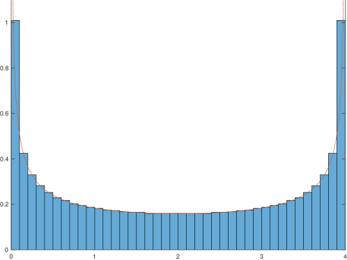
Figure 3: Histogram of (exact) eigenvalues of $(\textbf{1}_{2},n)$ for $n=4000$ mapped against $f(t)=(1/\pi)/\sqrt{t(4-t)}$ (in red).

From Theorem 3.2, we can fully realize the ESD of the $n=2$ case via the push-forward of the uniform map through the symbol, as seen in Figure 3. This is possible as a consequence of the corresponding weak limit asymptotic result from Theorem 3.2, since the Toeplitz operator in this case is Hermitian (and positive definite). For us this only applies when $m=2$ for $(\textbf{1}_{m},n)$, as seen starting for $m\geq 3$ then $(\textbf{1}_{m},n)$ is no longer Hermitian.

3.1.2 TPHT using $(\textbf{1}_{3},n)$

For fixed $m\geq 3$, then $T_{n}=(\textbf{1}_{m},n)$ has the associated symbol $\varphi(z)=z^{-1}(z+1)^{m}$ (which is not real-valued on $\mathbb{S}^{1}$) so that

$$\varphi(z)^{p}\cdot\frac{1}{z}=z^{-p-1}(z+1)^{mp}=\sum_{k=0}^{mp}\binom{mp}{k}z^{k-p-1}.$$

By (40),

(48) $$\lim_{n\to\infty}\frac{1}{n}\sum_{j=1}^{n}\lambda_{j}(T_{n})^{p}=\frac{1}{2\pi i}\int_{\mathbb{S}^{1}}\varphi(z)^{p}\ \frac{dz}{z}=\binom{mp}{p}.$$

For instance, for $m=p=3$, then $\binom{mp}{p}=84$. Comparing this to fixed computed values for again $n=10^{k}$ for $k=2,3,4$:

• For $n=100$, then $\frac{1}{n}\sum_{j=1}^{n}\lambda_{j}(T_{n})^{3}=83.4$

• For $n=1000$, then $\frac{1}{n}\sum_{j=1}^{n}\lambda_{j}(T_{n})^{3}=83.94$

• For $n=10,000$, then $\frac{1}{n}\sum_{j=1}^{n}\lambda_{j}(T_{n})^{3}=83.994$

Now for entire $f(z)=e^{z}$, then for $m=3$, applying Theorem 3.2 yields

(49) $$\frac{1}{2\pi}\int_{0}^{2\pi}f(\varphi(e^{i\theta}))\ d\theta =\sum_{k\geq 0}\frac{\binom{mk}{k}}{k!}\approx 169.249{=}\lim_{n\to\infty}\frac{1}{n}\sum_{j=1}^{n}f(\lambda_{j}(T_{n})).$$

This again similarly compares for computed values with fixed $n=10^{k}$ for $k=2,3,4$:

• For $n=100$, then $\frac{1}{n}\sum_{j=1}^{n}f(\lambda_{j}(T_{n}))\approx 166.85865$

• For $n=1000$, then $\frac{1}{n}\sum_{j=1}^{n}f(\lambda_{j}(T_{n}))\approx 169.01002$

• For $n=10,000$, then $\frac{1}{n}\sum_{j=1}^{n}f(\lambda_{j}(T_{n}))\approx 169.22516$

Remark 3.3.

A followup study might examine explicit properties for the associated limiting spectral measure associated with $(\textbf{1}_{m},n)$. This can include deriving a closed form for the limiting spectral measure, as realized through an associated Hypergeometric function for the associated Laplace transform along with deriving explicit convergence rates, which the preceding examples indicate to be $O(\frac{1}{n})$ for the fixed moment cases.

4 Spectral theory of TPH exemplified through TPHT

The results up to this point show that the spectrum of an element of TPHT coincides with that for all elements in the isospectral class $\mathcal{O}_{\Lambda}$ of TPH containing that Toeplitz element. Thus spectral results about a TPHT element hold for the full class $\mathcal{O}_{\Lambda}$ it represents. (We remind that while the eigenvalues are the same, the eigenvectors within this class change while still preserving the general oscillation properties described in Section 2.2.)

4.1 Numerics: Motivation

We will consider the asymptotic spectral properties of TPHT matrices with random symbols. The motivation for this comes from a number of directions. For the first of these we recall that in [8], Dumitriu and Edelman showed that the GOE($n$) random matrix ensemble ($n\times n$ symmetric matrices with independent normal entries modulo the symmetry) has a Householder tridiagonalization whose entries are independent with distributions

$$\alpha_{j}\sim\mathcal{N}(0,2)\qquad\mbox{and}\qquad\beta_{j}\sim\chi^{2}_{n-j},$$

where $\alpha_{j}$ are the diagonal entries of the tridiagonalization and the symmetric entries just above and below the diagonal are distributed as $\sqrt{\beta_{j}}$. They further showed that this induces, on the eigenvalues of $X\sim\operatorname{GOE}(n)$, a joint probability distribution of the form (up to a normalization)

(50) $$P(\lambda_{1},\dots,\lambda_{n})=\ \exp\left(-\frac{1}{4}\sum_{k=1}^{n}\lambda_{k}^{2}\right)\prod_{i<j}|\lambda_{j}-\lambda_{i}|.$$

It is a straightforward exercise to check that this distribution is the Radon-Nikodym derivative of the invariant measure associated to the Hamiltonian dynamics of the classical Toda Lattice. This observation has led to a growth of focus on the Toda lattice as a model for hydrodynamic limits of more general lattice systems (e.g., [30, 33]). The ensemble studied in this paper provides a basis for studying generalized hydrodynamics for the integrable full Toda lattice systems (cf. [14]).

In another direction, Freeman Dyson introduced a matrix model related to the GUE($n$) random matrix ensemble ($n\times n$ Hermitian matrices with independent complex normal entries, modulo the Hermitian symmetry) [9]. His generalization amounted to replacing the normal entries by Brownian motions. The resulting ensemble/process is nowadays referred to as Dyson Brownian motion (DBM) with principal interest being in the process it induces on eigenvalues. This is described by the following system of stochastic ODE’s.

(51) $$d\lambda_{k}(t)=dB_{k}+\sum_{j\neq k}\frac{1}{\lambda_{k}(t)-\lambda_{j}(t)}dt,\,\,\,\,k=1,\dots,n.$$

DBM has been intensively studied over the past few decades. If the eigenvalues are initially ordered as $\lambda_{1}>\cdots>\lambda_{n}$, then, with probability 1, this ordering will be maintained under the evolution. One celebrated result is that the distribution of the largest eigenvalue, $\lambda_{1}$, limits as $n\to\infty$ to the Tracy-Widom distribution, which is built from a particular solution of the Painlevé II equation [20]. A connection for all of this with Toda was found by O’Connell, who showed, effectively, that (51) also arises as the zero temperature limit of a Markovian stochastic process whose infinitesimal generator comes from the quantum Toda lattice [28]. The stochastic process considered by O’Connell is naturally expressed in terms of TPH matrices with random entries that are of log-normal type. For that reason we will consider here cases where the coefficients $a_{i}$ in the symbol $\varphi$ are independent, positive random variables. We will, in particular, consider the case where the $a_{i}$ are independent log-normal.

4.2 Numerics with log-normal symbol coefficients

We begin with the general case where the coefficients of the Toeplitz symbol, $a_{i}$, are independent random variables. For such random symbols, it is of interest to compute distributional properties for the associated $p$-part of the random symbol coefficients. As was seen in (40)-(45) this should correspond to the asymptotic limit for the $p^{th}$ moment of the ESD for the Toeplitz matrices associated to the random symbol. For example, the first moment computations for the $p$-part of the symbol $\varphi(t)$ has mean $\mu_{p}^{(m)}$ given by

$$\mu_{p}^{(m)} =\mathbb{E}\left(\sum_{\sum i_{j}=p}{p\choose i_{1}}\cdots{p\choose i_{m}}a_{1}^{i_{1}}\cdots a_{m}^{i_{m}}\right).=\sum_{\sum i_{j}=p}{p\choose i_{1}}\cdots{p\choose i_{m}}\mathbb{E}(a_{1}^{i_{1}})\cdots\mathbb{E}(a_{m}^{i_{m}})$$

As already mentioned, we will primarily specialize to the case where the $a_{i}$ are log-normal. Recall that a random variable $X$ is called log-normal if $\log X$ is normally distributed. The density function is

$$\frac{1}{x\sigma\sqrt{2\pi}}\exp{\frac{(\log x-\mu)^{2}}{2\sigma^{2}}}$$

where $\mu$ and $\sigma^{2}$ are the mean and variance of the underlying normal distribution.

We will restrict attention to the case where $\mu=0$ for all the random variables considered but the $\sigma$ may vary from one random variable to another. It follows that the terms, $a_{1}^{i_{1}}\cdots a_{m}^{i_{m}}$, in the summand in (45) are log-normal with underlying parameters $\mu=0$ and $\sigma^{2}=\sum_{j=1}^{m}i_{j}^{2}\sigma_{j}^{2}$ where $\sigma^{2}_{j}$ is the underlying variance of $a_{j}$; however, (45) is then a linear combination of (dependent) log-normals but is not itself log-normal.

More precisely, in the case where the $a_{i}$ are independent log-normals with underlying parameters $\mu=0$ and variance $\sigma_{i}^{2}$, one has

(52) $$\mu_{p}^{(m)} =\sum_{\sum i_{j}=p}{p\choose i_{1}}\cdots{p\choose i_{m}}\exp\left(\frac{i_{1}^{2}\sigma_{1}^{2}}{2}\right)\cdots\exp\left(\frac{i_{m}^{2}\sigma_{m}^{2}}{2}\right)$$

(53) $$=\sum_{\sum i_{j}=p}{p\choose i_{1}}\cdots{p\choose i_{m}}\exp\left(\frac{\sum_{j=1}^{m}i_{j}^{2}\sigma_{j}^{2}}{2}\right).$$

In the independent and identically distributed (iid) log-normal case, where all $\sigma_{i}=\sigma$ are equal, this reduces to

$$\mu_{p}^{(m)}=\sum_{\sum i_{j}=p}{p\choose i_{1}}\cdots{p\choose i_{m}}\exp\left(\frac{\sigma^{2}\sum_{j=1}^{m}i_{j}^{2}}{2}\right).$$

Using standard norm equivalence relations for $\sum_{j=1}^{m}i_{j}=p$, we have the inequalities

$$\frac{p^{2}}{m}=\frac{1}{m}\left(\sum_{j=1}^{m}i_{j}\right)^{2}\leq\sum_{j=1}^{m}i_{j}^{2}\leq\left(\sum_{j=1}^{m}i_{j}\right)^{2}=p^{2}$$

Using also the fact

(54) $$\binom{mp}{p}=\sum_{\sum i_{j}=p}{p\choose i_{1}}\cdots{p\choose i_{m}},$$

(this follows from a trivial combinatorial argument of counting the number of ways of placing $p$ balls into $mp$ bins in two ways) which gives the explicit expected $p^{th}$ part coefficient for the right hand side (RHS) of the ESD limit of $(\boldsymbol{1}_{m},n)$ (see (48)), we have

(55) $$\binom{mp}{p}\exp\left(\frac{\sigma^{2}p^{2}}{2m}\right)\leq\mu_{p}^{(m)}\leq\binom{mp}{p}\exp\left(\frac{\sigma^{2}p^{2}}{2}\right).$$

These comprise the upper and lower bounds found in Figures 4 to 7 using $\sigma=1$ (note the logarithmic scaling then skews the location of the mean relative to the median); the other (even lower) bound shown is the associated limiting spectral moment for $(\textbf{1}_{m},n)$ from (48) and (54), which appears to be a good estimator for the sample median.

Note the above lower bound could also be achieved using a Lagrange multiplier method to minimize the objective function $f(i_{1},\ldots,i_{m})=\sum_{j=1}^{m}i_{j}^{2}$ given the constraint $\sum_{j=1}^{m}i_{j}=p$. A similar computation now using different $\sigma_{1},\ldots,\sigma_{m}$ (so a new objective function $f(i_{1},\ldots,i_{m})=\sum_{j=1}^{m}i_{j}^{2}\sigma_{j}^{2}$) yields the lower bounds

(56) $$\binom{mp}{p}\exp\left(\frac{p^{2}}{2\sum_{j=1}^{m}1/\sigma_{j}^{2}}\right)\geq\binom{mp}{p}\exp\left(\frac{p^{2}\min_{i}\sigma_{i}^{2}}{2m}\right),$$

while a trivial upper bound holds with

(57) $$\binom{mp}{p}\exp\left(\frac{p^{2}\max_{i}\sigma_{i}^{2}}{2}\right).$$

(It is straightforward to also calculate the variance of these $p$-part random symbol coefficients, but we will not make use of that here.)

4.2.1 Numerical experiments

We now turn to the numerical simulation of the $p^{th}$ moments of the spectrum of $(\textbf{a}_{m},n)$ for large $n$ and where $\textbf{a}_{m}\in\mathbb{R}^{m}$ with iid standard log-normal components $a_{i}$. We match both the large $n$ matrix values from the left hand side (LHS) of Theorem 3.1 against the asymptotic distributions that are given by the RHS. We also sample the case where the $a_{i}$ are iid exponential distributions with unit mean. All experiments are run in MATLAB with double precision (i.e., machine precision using $\varepsilon_{\operatorname{machine}}=2^{-52}\approx 2.2\cdot 10^{-16}$).

For our experiments, we run 100,000 samples of both the LHS and RHS distributions associated with the $p^{th}$ random symbol coefficients for $(\textbf{a}_{m},n)$, where the vector $\textbf{a}_{m}$ are generated using built-in MATLAB functions to generate normal and exponential vectors (e.g., exp(randn(3,1)) is a standard log-normal vector in $\mathbb{R}^{3}$). To ease the following discussion, we focus our experiments on using only $m=3,10$ input parameters and moments $p=3,20$, as we feel these are representative of performance with other fixed combinations.

To sample the LHS matrix ensemble, we compute $\frac{1}{n}\operatorname{Tr}(A^{p})$ for iid $n\times n$ $A\sim(\textbf{a}_{m},n)$, where $A$ is formed using custom MATLAB code that generates a Toeplitz Hessenberg banded matrix whose input diagonals are the elementary symmetric polynomials associated with the random symbol vector $\mathbf{a}_{m}$. This follows since $\frac{1}{n}\operatorname{Tr}(A^{p})=\frac{1}{n}\sum_{k=1}^{n}\lambda_{k}(A)^{p}$. To simplify discussion, we fix $n=100$ for our experiments; empirically, the convergence in Theorem 3.1 is generally fast (cf. discussion below that compares LHS and RHS empirical cumulative distribution functions (CDFs) for $n=10$), so choosing $n=100$ is sufficient for comparisons.

For each sample of the RHS asymptotic $p^{th}$ moment, we form a $(p+1)\times(p+1)$ matrix that is generated by using the symbol generated with $a_{i}$ iid from a prescribed distribution but now interpreted as a matrix equation, replacing $t$ with $\epsilon^{T}=\sum_{i=1}^{p}\textbf{E}_{i,i+1}$, where now the $p^{th}$ part of the symbol then aligns with the $p^{th}$ lower diagonal. For example, we form $B=\prod_{i=1}^{n}(\textbf{I}+a_{i}\epsilon)\in M_{p+1}(\mathbb{R})$, and then store only $B_{p+1,1}$ for each sample.

Remark 4.1.

There is a choice on how to sample the right-hand side of Theorem 3.1 in comparison to the LHS. Forming $B$ as outlined above, one could simultaneously sample both the LHS and RHS samples using the same generated $a_{i}$ values, or each side can be sampled independently. Figures 4 to 7 choose independent samples for each side.

Figures 4 to 7 show the summary histogram output for the 100,000 samples on a logarithmic scale for each combination of $m=3,10$ (inputs), $p=5,20$ (moments) and $a_{i}$ iid (standard log-normal versus exponential with unit mean). For comparison for each model, the associated asymptotic $p^{th}$ moment for $(\textbf{1}_{m},n)$, i.e., $\binom{mp}{p}$, is shown with a vertical yellow line. Also included are both bounds from (55) (i.e., $\binom{mp}{p}\exp\left(\frac{p^{2}}{2m}\right)$ and $\binom{mp}{p}\exp\left(\frac{p^{2}}{2}\right)$), which contain the mean in the iid standard log-normal case; the upper bound is omitted in the $p=20$ cases.

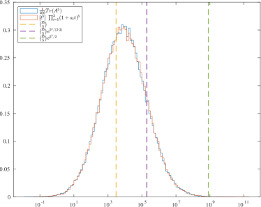
(a) Standard log-normal

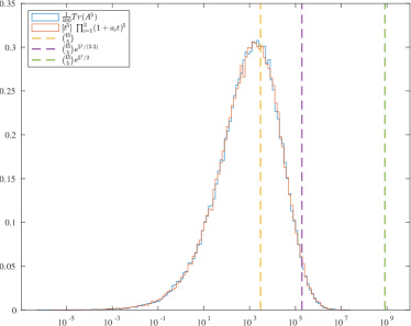
(b) Exponential

Figure 4: Computed $5^{th}$ moment for ESD for $A\sim(\textbf{a}_{3},100)$, where $\textbf{a}_{3}\in\mathbb{R}^{3}$ has iid (a) standard log-normal or (b) exponential with unit mean components, using 100,000 samples

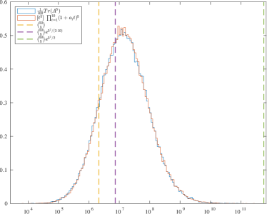
(a) Standard log-normal

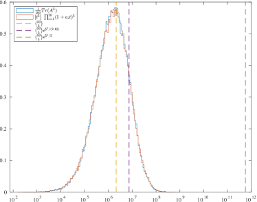
(b) Exponential

Figure 5: Computed $5^{th}$ moment for ESD for $A\sim(\textbf{a}_{10},100)$, where $\textbf{a}_{10}\in\mathbb{R}^{10}$ has iid (a) standard log-normal or (b) exponential with unit mean components, using 100,000 samples

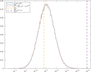
(a) Standard log-normal

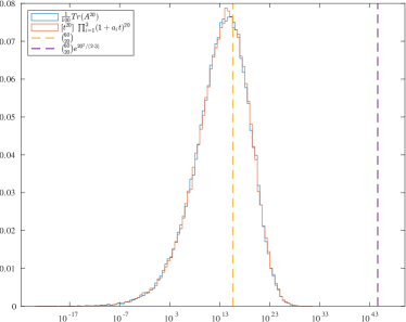
(b) Exponential

Figure 6: Computed $20^{th}$ moment for ESD for $A\sim(\textbf{a}_{3},100)$, where $\textbf{a}_{3}\in\mathbb{R}^{3}$ has iid (a) standard log-normal or (b) exponential with unit mean components, using 100,000 samples

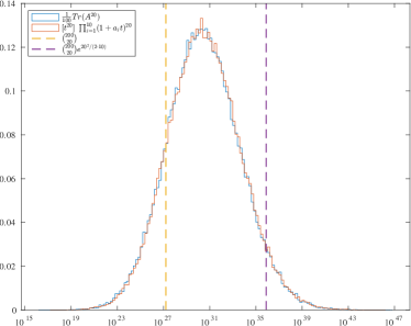
(a) Standard log-normal

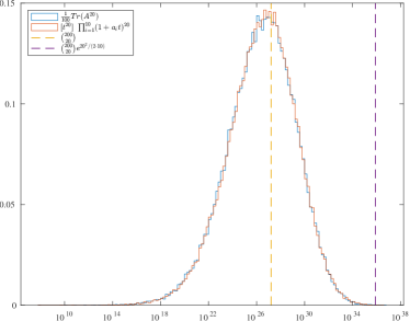
(b) Exponential

Figure 7: Computed $20^{th}$ moment for ESD for $A\sim(\textbf{a}_{10},100)$, where $(\textbf{a}_{10}\in\mathbb{R}^{10}$ has iid (a) standard log-normal or (b) exponential with unit mean components, using 100,000 samples

One quick take away for the standard log-normal maps from Figures 4, 5, 6, and 7 is the associated $p^{th}$ moments still exhibit log-normal behavior, as seen by a near normal curve using a logarithmic scaling. For comparison, the associated exponential maps show skewed behavior on the same scaling, which tend to also approach log-normal behavior for larger moments and number of input parameters (cf. Figure 7b). This suggests that even though no models are equal in distribution to a log-normal (even in the standard log-normal setup, then the associated $p^{th}$ moments are linear combinations of dependent log-normals), a universal behavior seems to limit toward a log-normal scheme. A followup study could focus on expanding these empirical findings.

For the $(\textbf{1}_{m},n)$ moment used for comparison in Figures 4, 5, 6, and 7, the $o(1)$ terms from the statement of Theorem 3.1 can be explicitly realized as $O(\frac{1}{n})$, as discussed previously. For example, for $A$ one of the $100\times 100$ matrices (out of $10^{5}$ total) used to generate the exponential LHS picture in Figure 4b, then $A^{3}$ has diagonal entries 1.1635 for indices 3 to 98, 1.1342 for indices 2 and 99, and 0.7202 for indices 1 and 100. Standard tools and nonparametric statistical tests can be used to compare the distributional properties for the LHS and RHS. For instance, the Kolmogorov-Smirnov (KS) distance between each empirical CDF (i.e., supnorm distance between both empirical CDFs) is a standard comparison tool for two distributions. For reference, we can consider 100,000 samples for each corresponding side of the $5^{th}$ moment with 3-inputs and $100\times 100$ matrices with iid standard log-normal entries using both potential sampling methods (cf. Remark 4.1). When comparing the LHS to the simultaneously sampled RHS random symbol, then the KS distance is 0.00185; when comparing the LHS to the independently sampled RHS random symbol (as in Figure 4a), then the KS distance is 0.00263. So these are very good matches already for $n=100$. If doing the same but now using only $10\times 10$ order matrices for the LHS, the match now has KS distances to the RHS simultaneous and independent sampling methods, respectively, of 0.01632 and 0.02062. This further justifies choosing $n=100$ for the above experiments, as $n=10$ already shows strong connections to the asymptotic picture.

4.3 Numerical Issues

Basak, Paquette and Zeitouni show that a small perturbed Toeplitz matrix has ESD that converges to the law of the symbol in probability [3]. This is exactly what we encounter using any computations in floating-point arithmetic of any fixed (non-exact) precision order. For example, this is what we see with Figures 8a and 8b when using the built-in eig function in MATLAB for $(\textbf{1}_{m},4000)$ for $m=3,8$ when using double precision, since the floating-point error matrix satisfies the hypotheses of their [3, Theorem 1]. With exact arithmetic, the eigenvalues of $T_{n}=(\textbf{1}_{m},n)$ are positive and distributed on the interval $[0,2^{m}]$; this follows since $T_{n}=(\textbf{1}_{m},n)$ has positive eigenvalues (it’s TP) that further satisfy

(58) $$\lambda_{\max}(T_{n})\leq\sigma_{\max}(T_{n})=\|T_{n}\|_{2}\leq\|T_{n}\|_{1}=\max_{j}\sum_{i}|(T_{n})_{ij}|=\sum_{j=0}^{m}\binom{m}{j}=2^{m}$$

(using the fact the $L^{1}$ induced matrix norm satisfies the max column sum property, while $T_{n}$ has binomial coefficients as its diagonal entries (cf. Section 3.1)).

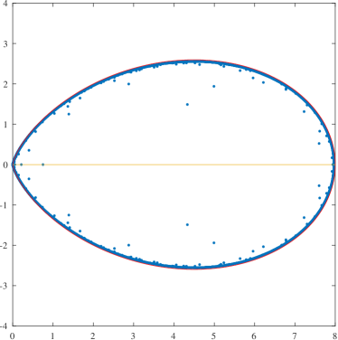
(a) $(\textbf{1}_{3},4000)$

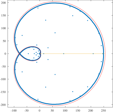
(b) $(\textbf{1}_{8},4000)$

Figure 8: Computed eigenvalues of $(\textbf{1}_{m},4000)$, mapped against $\varphi(e^{i\theta})$ for $\theta\in[0,2\pi)$ where $\varphi(z)=(1+z)^{m}/z$ is the (complex) symbol of the associated Toeplitz operator (in red) along with the interval $[0,2^{m}]$ (in yellow) for $m=3,8$.

Even though for our TPHT matrices we know the spectrum is real, the operator is not Hermitian for anything other than the tridiagonal case. Computations of TPHT spectra using default eig functions in MATLAB will similarly result in the accumulation of errors on the law of the symbol of the associated Toeplitz operator for $(\textbf{1}_{m},n)$ for sufficiently large $n$ when $m\geq 3$.

5 Conclusions and Further Directions

5.1 TPUT

As a point of comparison, there is an elegant characterization of TP, unipotent (bi-infinite) Toeplitz operators (TPUT) ultimately due to [1]. The result is

Theorem 5.1 ([1]).

The symbols of all lower unipotent Toeplitz operators that are TP have precisely the form

(59) $$\varphi(z)=1+x_{1}z+x_{2}z^{2}+\cdots=e^{\gamma z}\prod_{j\geq 1}\frac{1+a_{j}z}{1-b_{j}z}$$

where $a_{j},b_{j}$ are decreasing non-negative sequences in $\ell^{1}$ and $\gamma\geq 0$.

There is also a finite size analogue of Theorem 5.1 due to Rietsch [31], which states that the class of finite TPUT matrices is parameterized by polynomial symbols whose coefficients are quantum elementary symmetric polynomials as opposed to the ordinary symmetric polynomials of the bi-infinite case. Quantum elementary symmetric polynomials here are the coefficients of the characteristic polynomials of Hessenberg Jacobi matrices.

We note that by Theorem 2.6, the description of an element in $\mathcal{O}_{\Lambda}$ essentially reduces to a TP unipotent (TPU) element. Theorem 2.9 gives a precise characterization of the unique element of this class that is Toeplitz, when that element is TP. It will be of interest to study how these representative elements may be related to the TPUT results just mentioned.

5.2 Total Positivity of Additional LU dynamic Invariants

A remarkable property of TP matrices is that their Schur complements are also TP [2]. This has relevance for the complete integrability of the Full Kostant-Toda Lattice (cf. [12] and [10]). As explained in Section 2.2, this is a generalization of the well-known tridiagonal Toda lattice whose phase space is the entirety of the lower Hessenberg matrices. As is also mentioned in that section there is a discrete dynamics on this phase space, consistent with the Toda dynamics and which is equivalent to the dynamics of LU factorization [34]. The eigenvalues of a Hessenberg matrix are constants of motion. Additionally, the eigenvalues of certain of its Schur complements (known as Ritz values but also referred to as chops in the integrable systems literature [12]) are constants of motion in involution with the original eigenvalues. The results in this paper show that for the dynamics restricted to TPH, all of these eigenvalues are real with eigenvectors having the same oscillation properties as stated in Theorem 2.4.

5.3 Lusztig Parameters

In [14] a presentation of the just mentioned LU dynamics on TPH is presented in terms of the Lusztig parameters that were described in Section 2.4. One sees from this construction that a stochastic dynamics on TPH is natural to define by taking the Lusztig parameters to be independent log-normal random variables. (See Appendix B of [14].) The connection between this and the stochastic structure induced from the random symbols for TPHT discussed in the current paper will be taken up in future work.

5.4 Comparison to Symmetric Toeplitz Operators

It is interesting to compare our TPHT ensemble to Hermitian Toeplitz operators for which the Toeplitz matrix is symmetric. We saw an example of where the two coincide in section 3.1.1. As in that example the spectrum for Hermitian Toeplitz is always real (as for TPHT generally) but now the asymptotic density of the spectrum may be realized as the push-forward to $\mathbb{R}$ of Lebesgue measure on the circle under the symbol [4]. It is also the case that there is an analogue of the Full Kostant Toda lattice in which the phase space of Hessenberg matrices is replaced by real symmetric matrices. However in this symmetric case one does not have the same tight relation to Toeplitz matrices that was described in Section 2.1 and that underlies our spectral analysis of general TPH class. Nevertheless, the study of symmetric Toeplitz operators merits further investigation and will also be taken up elsewhere.

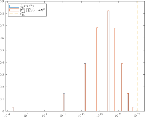
(a) Bernoulli

Figure 9: Computed $20^{th}$ moment for ESD for $A\sim(\textbf{a}_{10},100)$, where $\textbf{a}_{10}\in\mathbb{R}^{10}$ has iid Bernoulli($1/2$) components

5.5 Random Symbols for Discrete Distributions

Up to this point we have focused on random symbols associated to strictly positive continuous distributions. It is interesting to consider nonnegative discrete cases such as, for instance, $a_{i}\sim$ Bernoulli(q) iid. If we fix $m$ inputs, then $A\sim(\textbf{a}_{m},n)$, and $A$ is an TPHT matrix with $A=(\textbf{1}_{X},n)$ where $X\sim\operatorname{Binomial}(m,q)$. In this model, the $p^{th}$ moment $\mu_{p}^{(m)}$ can be determined by a calculation similar to that done for $(\textbf{1}_{m},n)$ in Section 3. So the symbol comprises a random variable that satisfies

(60) $$\mathbb{P}\left(\mu_{p}^{(m)}=\binom{pk}{p}\right)=\mathbb{P}(X=k)=\binom{m}{k}q^{k}(1-q)^{m-k}.$$

Hence, $\mu_{p}^{(m)}\sim\binom{pX}{p}$ for $X\sim\operatorname{Binomial}(m,q)$. Considering this setup, Figure 9 is a map using 100,000 samples of $(\textbf{a}_{10},100)$ for $a_{i}\sim\operatorname{Bernoulli}(\frac{1}{2})$ compared against the limiting law from Theorem 3.1. Note the $X=0$ case is excluded from the logarithmic scale histogram; of $100,000$ samples of ESD $20^{th}$ moments with input $\textbf{a}_{10}$, 100 resulted in $X=0$ compared to 979 that resulted in $X=1$ (the left-most bar in the histogram, since then $\binom{pX}{p}=\binom{p}{p}=1=10^{0}$). The upper bound for this model matches the limiting associated moment for $(\textbf{1}_{10},n)$ of $\binom{10p}{p}=\binom{200}{20}$, as shown by the dotted yellow line.

Appendix A Appendix: Normal Forms

There are several normal forms that play a role for the matrix ensembles considered in this paper. The first of these is the rational canonical normal form for general lower Hessenberg matrices: every Hessenberg matrix is conjugate to its companion matrix which is also of Hessenberg type. We will show that this conjugation is uniquely achieved by a specific lower unipotent matrix. The second normal form is a bidiagonal Hessenberg matrix which is also related to a given Hessenberg matrix by a unique lower unipotent matrix. Finally for the more restrictive TPHT class we give, in Appendix B, the proof of Theorem 2.9 which brings into play the Hessenberg-Toeplitz normal form.

A.1 Flag Manifolds: The Principal Embedding and the Companion Embedding

We recall the companion matrix for matrices with spectrum $\Lambda=(\lambda_{1},\ldots,\lambda_{n})$ :

(61) $$c_{\Lambda}=\left[\begin{array}[]{ccccc}0&1\\ &0&\ddots\\ &&\ddots&1\\ &&&0&1\\ -c_{0}&-c_{1}&\cdots&-c_{n-2}&-c_{n-1}\end{array}\right],$$

where $\prod\limits_{i=1}^{n}(x-\lambda_{i})=x^{n}+\sum_{i=0}^{n-1}c_{i}x^{i}$ is the characteristic polynomial for $\lambda$.

We also take $B_{+}$ to denote the group of invertible upper triangular matrices along with a distinguished principal nilpotent element,

$$\epsilon = \left(\begin{array}[]{ccccc}0&1&&&\\ &0&1&&\\ &&\ddots&\ddots&\\ &&&\ddots&1\\ &&&&0\end{array}\right).$$

In terms of this distinguished element we define

(63) $$\epsilon_{\Lambda}=\epsilon+\operatorname{diag}(\Lambda)=\left[\begin{array}[]{cccc}\lambda_{1}&1\\ &\lambda_{2}&\ddots\\ &&\ddots&1\\ &&&\lambda_{n}\end{array}\right].$$

In the work of [14, 29], the focus is on $\epsilon_{\Lambda}$, whereas the version used by [12] and [24] is $c_{\Lambda}$. The latter has the advantage of providing a unique representative that is independent of the choice of ordering on $\Lambda$.

We now recall a theorem essentially due to Kostant [24]:

Theorem A.1 ([12]).

For each $X\in\mathcal{O}_{\Lambda}$, there exists a unique lower unipotent $L\in N_{-}$, such that

(64) $$X=Lc_{\Lambda}L^{-1}.$$

The same statement holds (with a different $L\in N_{-}$) when $c_{\Lambda}$ is replaced by $\epsilon_{\Lambda}$ (with a specific ordering of $\Lambda$).

A key feature of this result is that $L$ is unique and so makes possible the following definition.

Definition A.2.

The companion embedding is the map $\kappa_{\Lambda}:\mathcal{O}_{\Lambda}\to{G}/B_{+}$ defined as follows: for $X\in\mathcal{O}_{\Lambda}$, if $X=Lc_{\Lambda}L^{-1}$, then

(65) $$\kappa_{\Lambda}(X)=L^{-1}\mod B_{+}.$$

Remark A.3.

An analogous embedding (described later in this section) can be performed using $\epsilon_{\Lambda}$ in place of $c_{\Lambda}$. We call this the principal embedding.

We now turn our attention to the $L$’s in both embeddings, finding explicit formulæ where possible and offering a means of translation between the two by expressing the relationship between the $L$’s corresponding to $\epsilon_{\Lambda}$ and to $c_{\Lambda}$.

Lemma A.4.

For each $n\in\mathbb{N}$, if $X$ is a tridiagonal $n\times n$ Hessenberg matrix, and for $1<k\leq n$,

$$\det(xI_{k-1}-X^{(k-1)})=x^{k-1}+\sum_{i=1}^{k-1}l_{ki}x^{i-1}$$

the $n\times n$ lower unipotent matrix $L=(l_{ij})_{i,j}$ defined by the above $n-1$ polynomials is the unique such matrix satisfying

$$L^{-1}XL=c_{X}$$

where $c_{X}$ is the companion matrix of $X$ (or $c_{\Lambda}$, where $\Lambda=\operatorname{Spec}(X)$), and where $X^{(k)}$ denotes the principal $k\times k$ submatrix of $X$.

Proof A.5.

We prove this by induction:
The base case of $n=1$ is trivial: $X=[a_{1}]$, $L=[1]$ and $c_{X}=[a_{1}]$ clearly satisfies $XL=Lc_{X}$.
Let us suppose the result holds for some $n\in\mathbb{N}$. To proceed, suppose $X$ is an $(n+1)\times(n+1)$ tridiagonal Hessenberg matrix. We make the key observation that if $L$ is the conjugating matrix for $X$, then $L^{(n)}$ is the conjugating matrix for $X^{(n)}$, which follows immediately from the definition of the $l_{ki}$’s. Thus, the induction hypothesis asserts

(66) $$X^{(n)}L^{(n)}=L^{(n)}c_{X^{(n)}}.$$

We impose a block structure on $X$:

$$X=\left[\begin{array}[]{c|c}X^{(n)}&\mathbf{e}_{n}\\ \hline\cr b_{n}\mathbf{e}_{n}^{T}&a_{n+1}\end{array}\right]$$

where $\mathbf{e}_{n}$ is the last column of the $n\times n$ identity matrix.

We impose the analogous block structure on $L$:

$$L=\left[\begin{array}[]{c|c}L^{(n)}&0\\ \hline\cr\mathbf{v}^{T}&1\end{array}\right]$$

where $\mathbf{v}=[l_{n+1,1}~{}l_{n+1,2}~{}\cdots~{}l_{n+1,n}]$.

Let $c=L^{-1}XL$ with block structure $c=\left[\begin{array}[]{c|c}A&\mathbf{p}\\ \hline\cr\mathbf{q}^{T}&r\end{array}\right]$. Since $XL=Lc$, one obtains the following equation from the top-left block:

(67) $$X^{(n)}L^{(n)}+\mathbf{e}_{n}\mathbf{v}^{T}=L^{(n)}A,$$

with $A$ an $n\times n$ matrix.

By the invertibility of $L^{(n)}$, there can be only one $A$ satisfying this equation.

Claim. $A=\epsilon_{n}$, where $\epsilon_{n}$ is the $n\times n$ matrix with $1$’s on the superdiagonal and zeroes elsewhere. This $\epsilon_{n}$ is not to be mistaken with $\epsilon_{\Lambda}$. If $d_{\Lambda}=\text{diag}(\lambda_{1},\ldots,\lambda_{n})$, then $\epsilon_{\Lambda}=d_{\Lambda}+\epsilon_{n}$.
Proof of Claim. Using the induction hypothesis, and plugging in $A=\epsilon_{n}$, Equation 67 becomes

(68) $$L^{(n)}c_{X^{(n)}}+\mathbf{e}_{n}\mathbf{v}^{T}=L^{(n)}\epsilon_{n},$$

or, equivalently,

(69) $$L^{(n)}(\epsilon_{n}-c_{X^{(n)}})=\mathbf{e}_{n}\mathbf{v}^{T}.$$

Evaluating both sides, one obtains

(70) $$\left[\begin{array}[]{cccc}0&0&\cdots&0\\ \vdots&&&\vdots\\ 0&0&\cdots&0\\ l_{n+1,1}&l_{n+1,2}&\cdots&l_{n+1,n}\end{array}\right]=\left[\begin{array}[]{cccc}0&0&\cdots&0\\ \vdots&&&\vdots\\ 0&0&\cdots&0\\ p_{0}&p_{1}&\cdots&p_{n-1}\end{array}\right]$$

where

$$\det(xI_{n}-X^{(n)})=x^{n}+\sum_{k=0}^{n-1}p_{k}x^{k}=x^{n}+\sum_{i=1}^{n}l_{n+1,i}x^{i-1}=x^{n}+\sum_{i=0}^{n-1}l_{n+1,i+1}x^{i}.$$

Hence, $p_{k}=l_{n+1,k+1}$ for $k=0,\ldots,n-1$. Thus, the ansatz of $A=\epsilon_{n}$ was consistent, which proves the claim. $\square$

Returning to (66), we turn our attention to the top-right block:

(71) $$\mathbf{e}_{n}=L^{(n)}\mathbf{p}.$$

Since $(L^{(n)})^{-1}$ is lower unipotent, $\mathbf{p}=(L^{(n)})^{-1}\mathbf{e}_{n}=\mathbf{e}_{n}$, since the $\mathbf{e}_{n}$ is also the last column of $(L^{(n)})^{-1}$.

One can conclude therefore that this matrix $c$, given by $L^{-1}XL$, is a companion matrix. Since $c$ is conjugate to $X$, and the characteristic polynomial is invariant under matrix conjugation, one must have that $c$ is indeed the companion matrix for $X$. This completes the induction step, proving the theorem.

This gives a means for computing $L^{-1}$ in the principal embedding.

Lemma A.6.

Let $X\in\mathcal{O}_{\Lambda}$, and let $L_{1}$ be defined as in Lemma A.4, and let $L_{2}$ be the lower unipotent matrix such that for $i>j$

(72) $$(L_{2})_{ij}=(-1)^{i+j}e_{j-i}(\lambda_{1},\ldots,\lambda_{i-1})$$

where $e_{j-1}$ is the $(j-i)$-th elementary symmetric polynomial

(73) $$e_{j-i}(\lambda_{1},\ldots,\lambda_{i-1})=\sum_{1\leq k_{1}<k_{2}<\cdots<k_{j-i}\leq n}\lambda_{k_{1}}\lambda_{k_{2}}\cdots\lambda_{k_{j-i}},$$

then $L=L_{2}L_{1}^{-1}$ satisfies $X=L^{-1}\epsilon_{\Lambda}L$.

Proof A.7.

This is a consequence of Lemma A.4. One has $X=L_{1}c_{\Lambda}L_{1}^{-1}$, and I claim that $c_{\Lambda}=L_{2}^{-1}\epsilon_{\Lambda}L_{2}$. Thus, $X=L_{1}L_{2}^{-1}\epsilon_{\Lambda}L_{2}L_{1}^{-1}$, and so $L=(L_{1}L_{2}^{-1})^{-1}=L_{2}L_{1}^{-1}$.

The claim itself is simply an application of Lemma A.4 since

(74) $$\tau_{k}(xI_{n}-\epsilon_{\Lambda})=x^{k}+\sum_{i=0}^{k-1}(-1)^{k+i}e_{k-i}(\lambda_{1},\ldots,\lambda_{k}).$$

When $\lambda_{i}\neq\lambda_{j}$ for all $i\neq j$, one can of course diagonalise any matrix in $\mathcal{O}_{\Lambda}$. The following result, which is an explicit form of Lemma 7 in [11], describes a diagonalisation of $\epsilon_{\Lambda}$.

Lemma A.8.

If $\lambda_{1},\ldots,\lambda_{n}$ are distinct, then one has $\epsilon_{\Lambda}=Ud_{\Lambda}U^{-1}$, where $U=(u_{ij})$ is the upper triangular matrix given by

$$u_{ij}=\prod_{k=1}^{i-1}(\lambda_{j}-\lambda_{k}),~{}~{}~{}1\leq i\leq j\leq n$$

and $d_{\Lambda}=\epsilon_{\Lambda}-\epsilon=\operatorname{diag}(\lambda_{1},\ldots,\lambda_{n})$.

Proof A.9.

The matrix $U$ is clearly invertible if and only if $\lambda_{i}\neq\lambda_{j}$ since

$$\det(U)=\prod_{i=1}^{n}\prod_{k=1}^{i-1}(\lambda_{i}-\lambda_{k})=\prod_{1\leq k<i\leq n}(\lambda_{i}-\lambda_{k}).$$

It just remains to show that $\epsilon_{\Lambda}U=Ud_{\Lambda}$. Let $u_{j}=(u_{ij})_{1\leq i\leq n}$ be the $j$-th column of $U$, then for $i<n$:

$$(\epsilon_{\Lambda}u_{j})_{i} =\sum_{k=1}^{n}(\epsilon_{\Lambda})_{ik}u_{kj}$$

$$=\lambda_{i}u_{ij}+u_{i+1,j}$$

$$=\lambda_{i}\prod_{k=1}^{i-1}(\lambda_{j}-\lambda_{k})+\prod_{k=1}^{i}(\lambda_{j}-\lambda_{k})$$

$$=(\lambda_{i}+\lambda_{j}-\lambda_{i})\prod_{k=1}^{i-1}(\lambda_{j}-\lambda_{k})$$

$$=\lambda_{j}\prod_{k=1}^{i-1}(\lambda_{j}-\lambda_{k})$$

$$=\lambda_{j}(u_{j})_{i}.$$

For $i=n$, we simply have

$$(\epsilon_{\Lambda}u_{j})_{n} =\lambda_{n}(u_{j})_{n}$$

$$=\left\{\begin{array}[]{cl}0&j<n\\ \lambda_{j}(u_{j})_{n}&j=n\end{array}\right.$$

$$=\lambda_{j}(u_{j})_{n}.$$

Thus, $\epsilon_{\Lambda}u_{j}=\lambda_{j}u_{j}$ for each $j$.

A final feature of these embeddings is that they provide a means of representing the eigenfunctions for Hessenberg matrices $X$ when the eigenvalues of $X$ are distinct.

Corollary A.10.

$$XL^{-1}U=L^{-1}Ud_{\Lambda}$$

where $L=L_{2}L_{1}^{-1}$ from Lemma A.6. In other words $L^{-1}U$ is the matrix of eigenfunctions for $X$ presented in LU-factorized form.

The proof is an immediate consequence of the previous two lemmas.

Appendix B Proof of Theorem 2.9

We recall the statement of the theorem and give its detailed proof.

Theorem 2.9. Let $T$ be an $n\times n$ TPHT matrix in $\mathcal{H}^{\geq 0}$, defined in Theorem 2.6. Then $T$ has the LU decomposition $T=LU$ where

$$(L)_{ij} =\left\{\begin{array}[]{cc}0&i<j\\ \frac{\tau_{\{i\}\cup[j-1]}^{\text{init}}(T)}{\tau_{[j]}^{\text{init}}(T)}&i\geq j\end{array}\right.$$

$$(U)_{ij} =\left\{\begin{array}[]{cc}\frac{\tau_{[i]}^{\text{init}}(T)}{\tau_{[i-1]}^{\text{init}}(T)}&i=j\\ 1&j=i+1\\ 0&\text{{otherwise.}}\end{array}\right.$$

Proof B.1.

We prove this by induction on $n$. To aid in the proof, for $n\in\mathbb{N}$, denote by $T_{n}$ the matrix given by

$$(T_{n})_{ij}=\left\{\begin{array}[]{cc}a_{i-j+1}&i\geq j\\ 1&j=i+1\\ 0&j>i+1\end{array}\right.=\left[\begin{array}[]{ccccc}a_{1}&1&0&\cdots&0\\ a_{2}&a_{1}&1&\ddots&\vdots\\ a_{3}&a_{2}&\ddots&\ddots&0\\ \vdots&\ddots&\ddots&\ddots&1\\ a_{n}&\cdots&a_{3}&a_{2}&a_{1}\end{array}\right].$$

If $n=1$, the theorem states that

$$T_{1}=[\,a_{1}\,]=[\,1\,]\,[\,\tau_{[1]}^{\text{init}}(T)\,]$$

which holds trivially. So, assume $n>1$. Now, observe that $T_{n}$ sits inside $T_{n+1}$ as its principal sub-matrix (top-left):

$$T_{n+1}=\left[\begin{array}[]{c|c}T_{n}&\mathbf{e}_{n}\\ \hline\cr[a_{n+1}~{}\cdots~{}a_{3}~{}a_{2}]&a_{1}\end{array}\right].$$

We assume that $T_{n}=L_{n}U_{n}$ where

$$(L_{n})_{ij} =\left\{\begin{array}[]{cc}0&i<j\\ \frac{\tau_{\{i\}\cup[j-1]}^{\text{init}}(T_{n})}{\tau_{[j]}^{\text{init}}(T_{n})}&i\geq j\end{array}\right.~{}~{}~{}=~{}~{}~{}~{}~{}\left\{\begin{array}[]{cc}0&i<j\\ \frac{\tau_{\{i\}\cup[j-1]}^{\text{init}}(T_{n+1})}{\tau_{[j]}^{\text{init}}(T_{n+1})}&i\geq j\end{array}\right.$$

$$(U_{n})_{ij} =\left\{\begin{array}[]{cc}\frac{\tau_{[i]}^{\text{init}}(T_{n})}{\tau_{[i-1]}^{\text{init}}(T_{n})}&i=j\\ 1&j=i+1\\ 0&\text{otherwise}\end{array}\right.~{}~{}~{}=~{}~{}~{}~{}~{}\left\{\begin{array}[]{cc}\frac{\tau_{[i]}^{\text{init}}(T_{n+1})}{\tau_{[i-1]}^{\text{init}}(T_{n+1})}&i=j\\ 1&j=i+1\\ 0&\text{otherwise}\end{array}\right..$$

Note the second equality in each line is due to $T_{n}$ sitting inside $T_{n+1}$ as its principal sub-matrix. Because of this, the rest of this proof shall write $\tau^{\text{init}}_{S}$ for $\tau^{\text{init}}_{S}(T_{n+1})$.
Now consider the LU decommposition of $T_{n+1}$ in $2\times 2$ block form with the principal $n\times n$ sub-matrix as a block:

$$T_{n+1}=L_{n+1}U_{n+1}=\left[\begin{array}[]{c|c}L_{n+1}^{(n)}&\mathbf{0}_{n}\\ \hline\cr\mathbf{p}^{T}&1\end{array}\right]\left[\begin{array}[]{c|c}U_{n+1}^{(n)}&\mathbf{q}\\ \hline\cr\mathbf{0}_{n}^{T}&r\end{array}\right]=\left[\begin{array}[]{c|c}L_{n+1}^{(n)}U_{n+1}^{(n)}&L_{n+1}^{(n)}\mathbf{q}\\ \hline\cr\mathbf{p}^{T}U_{n+1}^{(n)}&\mathbf{p}^{T}\mathbf{q}+r\end{array}\right]$$

where $A^{(n)}$ denotes the principal $n\times n$ sub-matrix.
By uniqueness of the LU decomposition, this implies that $L_{n+1}^{(n)}=L_{n}$ and $U_{n}=U_{n+1}^{(n)}$, which gives a nesting of LU decompositions for the sequence of matrices $(T_{n})_{n\in\mathbb{N}}$.
To see how the LU decomposition for $T_{n+1}$ relates to that of $T_{n}$, we need to solve the following for $\mathbf{p}$, $\mathbf{q}$ and $r$:

$$L_{n}\mathbf{q}=\mathbf{e}_{n},~{}~{}~{}~{}~{}\mathbf{p}^{T}U_{n}=[a_{n+1}~{}\cdots~{}a_{3}~{}a_{2}],~{}~{}~{}~{}~{}\mathbf{p}^{T}\mathbf{q}+r=a_{1}.$$

We immediately have $\mathbf{q}=L_{n}^{-1}\mathbf{e}_{n}=\mathbf{e}_{n}$ since $L_{n}$ and its inverse is lower unipotent.
We claim $\mathbf{p}^{T}=[p_{1}~{}p_{2}~{}\cdots~{}p_{n}]$ with $p_{j}=\frac{\tau^{\text{init}}_{\{n+1\}\cup[j-1]}}{\tau^{\text{init}}_{[j]}}$ satisfies $\mathbf{p}^{T}U_{n}=[a_{n+1}~{}\cdots~{}a_{3}~{}a_{2}]$. Let us multiply this out formally

$$(\mathbf{p}_{n}^{T}U_{n})_{1j} =\sum_{k=1}^{n}(\mathbf{p}_{n}^{T})_{1k}(U_{n})_{kj}$$

$$=\left\{\begin{array}[]{cc}\left(\frac{\tau^{\text{init}}_{\{n+1\}}}{\tau^{\text{init}}_{[1]}}\right)\tau^{\text{init}}_{[1]}&j=1\\ \frac{\tau^{\text{init}}_{\{n+1\}\cup[j-2]}}{\tau^{\text{init}}_{[j-1]}}\cdot 1+\frac{\tau^{\text{init}}_{\{n+1\}\cup[j-1]}}{\tau^{\text{init}}_{[j]}}\cdot\frac{\tau^{\text{init}}_{[j]}}{\tau^{\text{init}}_{[j-1]}}&1<j\leq n\end{array}\right.$$

$$=\left\{\begin{array}[]{cc}\tau^{\text{init}}_{\{n+1\}}&j=1\\ \frac{\tau^{\text{init}}_{\{n+1\}\cup[j-2]}+\tau^{\text{init}}_{\{n+1\}\cup[j-1]}}{\tau^{\text{init}}_{[j-1]}}&1<j\leq n\end{array}\right..$$

The first part satisfies $\tau^{\text{init}}_{\{n+1\}\cup[j-2]}=a_{n+1}$ simply because this is the minor determinant of the $1\times 1$ sub-matrix of $T_{n+1}$ in the last row of the first column.
It now remains to show that

$$\frac{\tau^{\text{init}}_{\{n+1\}\cup[j-2]}+\tau^{\text{init}}_{\{n+1\}\cup[j-1]}}{\tau^{\text{init}}_{[j-1]}}=a_{n+2-j},~{}~{}~{}~{}~{}\text{for}~{}~{}1<j\leq n.$$

But note that this is equivalent to

$$\tau^{\text{init}}_{\{n+1\}\cup[j-1]}=a_{n+2-j}\cdot\tau^{\text{init}}_{[j-1]}-\tau^{\text{init}}_{\{n+1\}\cup[j-2]}.$$

This is true because the left-hand side is given by

$$\tau^{\text{init}}_{\{n+1\}\cup[j-1]} =\det((T_{n+1})_{\{n+1\}\cup[j-1],[j]})$$

$$=\det\left[\begin{array}[]{ccccc}a_{1}&1&0&\cdots&0\\ a_{2}&a_{1}&\ddots&\ddots&\vdots\\ \vdots&\ddots&\ddots&\ddots&\vdots\\ a_{j-1}&\cdots&a_{2}&a_{1}&1\\ \hline\cr a_{n+1}&a_{n}&a_{n-1}&\cdots&a_{n+2-j}\end{array}\right]$$

so the desired equality is seen as the cofactor expansion down the last column in the above matrix.
Finally, we need to show that $\mathbf{p}^{T}\mathbf{q}+r=a_{1}$ implies $r=\frac{\tau^{\text{init}}_{[n+1]}}{\tau^{\text{init}}_{[n]}}$. Since we know $\mathbf{p}$ and $\mathbf{q}$, we can compute this directly:

$$r =a_{1}-\mathbf{p}^{T}\mathbf{q}$$

$$=a_{1}-\mathbf{p}^{T}\mathbf{e}_{n}$$

$$=a_{1}-p_{n}$$

$$=a_{1}-\frac{\tau^{\text{init}}_{\{n+1\}\cup[n-1]}}{\tau^{\text{init}}_{[n]}}$$

$$=\frac{a_{1}\cdot\tau^{\text{init}}_{[n]}-\tau^{\text{init}}_{\{n+1\}\cup[n-1]}}{\tau^{\text{init}}_{[n]}}$$

$$=\frac{\tau^{\text{init}}_{[n+1]}}{\tau^{\text{init}}_{[n]}}$$

where the last equation follows by considering the cofactor expansion down the last column of $T_{n+1}$.

References

- [1] M. Aissen, A. Edrei, I. J. Schoenberg, and A. Whitney, On the generating functions of totally positive sequences, Proceedings of the National Academy of Sciences - PNAS, 37 (1951), p. 303–307, https://doi.org/10.1073/pnas.37.5.303.
- [2] T. Ando, Totally positive matrices, Lin. Alg. and its Appl., 90 (1987), pp. 165–219, https://doi.org/10.1016/0024-3795(87)90313-2.
- [3] A. Basak, E. Paquette, and O. Zeitouni, Spectrum of random perturbations of Toeplitz matrices with finite symbols, Trans. Amer. Math. Soc., 373 (2020), pp. 4999–5023, https://doi.org/10.1090/tran/8040.
- [4] A. Böttcher and S. M. Grudsky, Spectral properties of banded Toeplitz matrices, SIAM, 2005.
- [5] A. Böttcher and B. Silbermann, Introduction to Large Truncated Toeplitz Matrices, Springer New York, New York, NY, 1 ed., 1998, https://doi.org/10.1007/978-1-4612-1426-7.
- [6] C. W. Cryer, Some properties of totally positive matrices, Lin. Alg. and its Appl., 15 (1976), pp. 1–25, https://doi.org/https://doi.org/10.1016/0024-3795(76)90076-8, https://www.sciencedirect.com/science/article/pii/0024379576900768.
- [7] J. Demmel and P. Koev, The accurate and efficient solution of a totally positive generalized Vandermonde linear system, SIAM J. Matrix Anal. Appl., 27 (2005), pp. 142–152, https://doi.org/10.1137/S0895479804440335.
- [8] I. Dumitriu and A. Edelman, Matrix models for beta ensembles, J. Math. Phys., 43 (2002), p. 5830–5847, https://doi.org/10.1063/1.1507823.
- [9] F. J. Dyson, A Brownian‐motion model for the eigenvalues of a random matrix, J. of Math. Phys., 3 (1962), p. 1191–1198, https://doi.org/10.1063/1.1703862.
- [10] N. M. Ercolani, The Poisson geometry of Plancherel formulas for triangular groups, Physica. D, 453 (2023), p. 133801, https://doi.org/10.1016/j.physd.2023.133801.
- [11] N. M. Ercolani, H. Flaschka, and L. Haine, Painlevé’ Balances and Dressing Transformations, Springer US, Boston, MA, 1991, p. 249–260, https://doi.org/10.1007/978-1-4899-1158-2_16.
- [12] N. M. Ercolani, H. Flaschka, and S. Singer, The Geometry of the Full Kostant-Toda Lattice, Birkhäuser Boston, Boston, MA, 1993, p. 181–225, https://doi.org/10.1007/978-1-4612-0315-5_9.
- [13] N. M. Ercolani and K. T.-R. McLaughlin, Asymptotics and integrable structures for biorthogonal polynomials associated to a random two-matrix model, Physica. D, 152 (2001), p. 232–268, https://doi.org/10.1016/S0167-2789(01)00173-7.
- [14] N. M. Ercolani and J. Ramalheira-Tsu, Lusztig factorization dynamics of the full Kostant–Toda lattices, Mathematical Physics, Analysis, and Geometry, 26 (2023), https://doi.org/10.1007/s11040-022-09444-3.
- [15] S. Fomin and A. Zelevinsky, Total positivity: Tests and parametrizations, Math Intelligencer, (2000), pp. 22–33, https://doi.org/10.1007/BF03024444.
- [16] J. Francis, The QR transformation, I, The Computer Journal, 4 (1961), pp. 265–271, https://doi.org/10.1093/comjnl/4.3.265.
- [17] J. Francis, The QR transformation, II, The Computer Journal, 4 (1962), pp. 265–271, https://doi.org/10.1093/comjnl/4.4.332.
- [18] A. Fukuda, E. Ishiwata, Y. Yamamoto, M. Iwasaki, and Y. Nakamura, Integrable discrete hungry systems and their related matrix eigenvalues, Annali di matematica pura ed applicata, 192 (2013), p. 423–445, https://doi.org/10.1007/s10231-011-0231-0.
- [19] M. Gasca and J. M. Peña, Chapter: Neville Elimination and Approximation Theory, In: Approximation Theory, Wavelets and Applications, Springer Netherlands, Dordrecht, 1995, pp. 131–151, https://doi.org/10.1007/978-94-015-8577-4_8z.
- [20] J. Gravner, C. A. Tracy, and H. Widom, Limit theorems for height fluctuations in a class of discrete space and time growth models, J. of Stat. Phys., 102 (2001), pp. 1085–1132, https://doi.org/10.1023/A:1004879725949, https://doi.org/10.1023/A:1004879725949.
- [21] U. Grenander, G. Szegő, and M. Kac, Toeplitz forms and their applications, Physics Today, 11 (1958), p. 38, https://doi.org/10.1063/1.3062237.
- [22] B. Gustafsson, H.-O. Kreiss, and A. Sundström, Stability theory of difference approximations for mixed initial boundary value problems. ii, Mathematics of Computation, 26 (1972), p. 649–686, https://doi.org/10.1090/S0025-5718-1972-0341888-3.
- [23] P. Koev, Accurate computations with totally nonnegative matrices, SIAM J. Matrix Anal. Appl., 29 (2007), pp. 731–751, https://doi.org/10.1137/04061903X.
- [24] B. Kostant, On Whittaker vectors and representation theory, Inventiones Mathematicae, 48 (1978), p. 101–184, https://doi.org/10.1007/BF01390249.
- [25] V. N. Kublanovskaya, On some algorithms for the solution of the complete eigenvalue problem, USSR Comp. Math. and Math. Phy., 1 (1961), pp. 265–271, https://doi.org/10.1016/0041-5553(63)90168-X.
- [26] C. Lanczos, An iteration method for the solution of the eigenvalue problem of linear differential and integral operators, J. of Research of the Nat. Bur. of Stand., 45 (2001), pp. 255–282, https://doi.org/10.6028/jres.045.026.
- [27] D. Mackey, N. Mackey, and S. Petrovic, Is every matrix similar to a Toeplitz matrix?, Lin. Alg. and its Appl., 297 (1999), pp. 87–105, https://doi.org/https://doi.org/10.1016/S0024-3795(99)00131-7, https://www.sciencedirect.com/science/article/pii/S0024379599001317.
- [28] N. O’Connell, Directed polymers and the quantum Toda lattice, The Ann. of Prob., 40 (2012), p. 437–458, https://doi.org/10.1214/10-AOP632. IMS-AOP-AOP632.
- [29] N. O’Connell, Geometric RSK and the Toda lattice, Illinois J. of Math., 57 (2013), https://doi.org/10.1215/ijm/1415023516.
- [30] J. A. Ramírez, B. Rider, and B. Virág, Beta ensembles, stochastic Airy spectrum, and a diffusion, J. of the AMS, 24 (2011), p. 919–944, https://doi.org/10.1090/S0894-0347-2011-00703-0.
- [31] K. Rietsch, Totally positive Toeplitz matrices and quantum cohomology of partial flag varieties, J. of the AMS, 16 (2003), p. 363–392, https://doi.org/10.1090/S0894-0347-02-00412-5.
- [32] Y. Saad and M. H. Schultz, GMRES: A generalized minimal residual algorithm for solving nonsymmetric linear systems, SIAM J. Sci. Stat. Comp., 7 (1986), pp. 856–869, https://doi.org/10.1137/0907058, https://arxiv.org/abs/https://doi.org/10.1137/0907058.
- [33] H. Spohn, Hydrodynamic equations for the Toda lattice, arXiv.org, (2021), https://doi.org/10.48550/arxiv.2101.06528.
- [34] W. Symes, Hamiltonian group actions and integrable systems, Physica D, 1 (1980), pp. 339–374, https://doi.org/https://doi.org/10.1016/0167-2789(80)90017-2, https://www.sciencedirect.com/science/article/pii/0167278980900172.