The Mixed Convex-Concave effect on the regularity of a Boltzmann solution

Abstract.

The geometric properties of domains are well-known to be crucial factors influencing the regularity of Boltzmann boundary problems. In the presence of non-convex physical boundaries, highly singular behaviors are investigated including the propagation of discontinuities [26] and Hölder regularity [30]. In this paper, we focus on studying the $C^{0,\frac{1}{4}-}$ Hölder regularity of the Boltzmann equation within concentric cylinders where both convex and concave features are present on the boundaries. Our findings extend the previous results of [30], which primarily addressed concavity while considering the exterior of convex objects.

1. Introduction

1.1. Background and Main results

The Boltzmann equation is a fundamental mathematical model for rarefied gases that accounts for collisions. It is expressed as a partial differential equation for the probability density function $F(t,x,v)\geq 0$, where $(t,x,v)$ represent time, space, and velocity, respectively. In terms of the probability density function $F(t,x,v)$, the Boltzmann equation is written as

$$\partial_{t}F+v\cdot\nabla_{x}F=Q(F,F),\ \ F(0,x,v)=F_{0}(x,v),$$ (1.1)

where $Q(F,F)$ is nonlinear quadratic collisional operator. The collision operator is written by

$$\begin{split}Q(F_{1},F_{2})&=\int_{\mathbb{R}^{3}}\int_{\mathbb{S}^{2}}B(v-u,\omega)[F_{1}(u^{\prime})F_{2}(v^{\prime})-F_{1}(u)F_{2}(v)]d\omega du\\ &:=Q_{\text{gain}}(F_{1},F_{2})-Q_{\text{loss}}(F_{1},F_{2}).\end{split}$$ (1.2)

(Here we abbreviate $(t,x)$ for notational convenience.) When two identical particle with velocities $u,v$ collide each other, we can describe post collisional velocities $u^{\prime}$ and $v^{\prime}$ as

$$u^{\prime}=u-((v-u)\cdot\omega)\omega,\quad\text{and}\quad v^{\prime}=v+((v-u)\cdot\omega)\omega$$

for $\omega\in\mathbb{S}^{2}$. We note that above expressions come from perfect elastic binary collision,

$$u+v=u^{\prime}+v^{\prime},\quad|u|^{2}+|v|^{2}=|u^{\prime}|^{2}+|v^{\prime}|^{2},$$

which means conservation of momentum and kinetic energy, respectively. Meanwhile, there are many mathematical models for collision kernel $B(v-u,\omega)$. In this paper, we consider hard sphere Boltzmann equation,

$$B(v-u,\omega)=|(v-u)\cdot\omega|.$$

We note that our result might be easily adapted to the Boltzmann equation with hard potential or Maxwellian molecule,

$$B(v-u,\omega)=|v-u|^{\gamma}b(\theta),\quad 0\leq\gamma<1,\quad 0\leq b(\theta)\leq C|\cos\theta|$$

for a general constant $C>0$.

Numerous articles have addressed the Boltzmann equation. In the seminal paper by Di Lion [8], the renormalization solution of the Boltzmann equation was investigated. For the global well-posedness of the Boltzmann equation and related models, Guo developed a high-order energy method in the vicinity of equilibrium, as detailed in [17, 19, 21]. In cases away from equilibrium, Desvillettes and Villani explored the convergence to equilibrium, assuming sufficiently smooth global solutions, as described in [7]. Additionally, we note the global well-posedness results presented in [16] concerning the non-cutoff Boltzmann equation.

Concerning general boundary condition problems, global well-posedness and regularity studies remained largely unknown until the work presented in [20]. We also refer [35, 25]. In this paper, an $L^{\infty}$ mild solution was proposed, and low regularity well-posedness was explored using a novel $L^{2}-L^{\infty}$ bootstrap argument. Subsequently, there has been widespread research on low regularity mild solution approaches. Collaborating with C. Kim, the second author in [28] extended the results of [20] from generalized analytic convex domains to general $C^{3}$ convex domains with specular boundary conditions. Moreover, the strong convexity assumptions on the boundary were relaxed to include some general non-convex domains in [29, 32].

For the non-cutoff Boltzmann equation, [1, 13] examined low regularity solutions in the presence of boundary conditions. It is also noteworthy to mention the large amplitude problem, where the small $L^{\infty}$ initial conditions in the aforementioned works were replaced with small $L^{p}$-type initial data, allowing for arbitrarily large $L^{\infty}$ amplitudes. For cases involving torus and whole space, refer to [10], and for boundary condition problems, see [12, 14]. Regarding the BGK equation, which is an essential relaxed model for the Boltzmann equation, recent research on large amplitude solutions can be found in [2].

The solutions presented in the aforementioned works are all considered to be low regularity mild solutions. It is widely believed that a solution to general Boltzmann boundary problems does not possess high-order regularity unless the boundary is flat. However, investigating the regularity of the Boltzmann solution in bounded domains is an extremely challenging research area.

In [23], Guo et al. examined the Boltzmann equation in a strictly convex domain with specular, bounce-back, and diffuse boundary conditions. They demonstrated that the first-order derivatives remain continuous away from the grazing set, where the backward-in-time linear trajectory tangentially intersects the boundary. In the context of non-convex domains, reference can be made to BV regularity results presented in [22] with diffuse reflection boundary conditions. In such cases, the convex geometry of the boundary plays a crucial role because the characteristics are differentiable within its domain.

In the context of the Boltzmann equation, the study of regularity in non-convex domains under specular reflection (billiard-like boundary conditions) had remained an open problem due to its challenging singularity issues associated with grazing collisions of trajectories (or billiard maps). However, in [30], Kim and Lee addressed the regularity of a Boltzmann solution in certain non-convex domains with specular reflection conditions. They established that a local-in-time solution outside a general convex object exhibits $C^{0,\frac{1}{2}-}_{x,v}$ regularity by investigating the averaging of grazing singularities in combination with the shift method.

The objective of our study in this paper is to investigate the regularity of a Boltzmann solution (1.1) within a cylindrical annulus domain under the specular reflection boundary condition. In the prior work [30], the domain considered was the outside of a convex obstacle, which, in geometrical terms, can be described as purely concave. Furthermore, when analyzing a billiard map in phase space, it is worth noting that at most one bounce can occur unless there is an external force.

In the context described above, the regularity result in [30] predominantly arises from the pure concavity of the domain. However, what happens when convexity is introduced into the domain? As demonstrated in [23, 33], convexity ensures the differentiability of the billiard map, but the billiard map’s escape behavior near the grazing regime is significantly slower compared to the concavity case. (It is important to mention that the rapid escape property of concavity is one of the key elements in [30].) Therefore, it becomes a natural and intriguing topic to investigate the regularity of a Boltzmann solution when a domain contains both convex and concave features.

For a general domain with both convexity and concavity, achieving precise derivative estimates appears to be a formidable task. Our chosen domain, ‘the concentric cylinder’, is a simple yet nontrivial domain of significance that encompasses both convex and concave elements. While the analysis of derivatives of the given billiard map may require substantial effort, we will leverage some valuable results from [23, 33] regarding characteristics to aid in our study.

First, we define concentric cylindrical annulus domain $\Omega$ and mild formulation of the Boltzmann equation as well as specular reflection boundary condition.

Definition 1.1 (cylindrical annulus domain).

We define a cylindrical annulus domain $\Omega$,

$$\Omega:=\{(\rho\cos\theta,\rho\sin\theta,z)|r<\rho<R,\;-\pi\leq\theta<\pi,\;-\infty<z<+\infty\},$$

for some positive constants $R,r\in\mathbb{R}^{+}$. For convenience, we assume that $R-r>1$, WLOG. Since the cross-section is circles, outward unit normal vector is defined by

$$n(x_{1},x_{2},x_{3})=\begin{cases}\frac{x_{p}}{|x|_{p}}\quad\text{for}\quad|x|_{p}=R,\\ -\frac{x_{p}}{|x|_{p}}\quad\text{for}\quad|x|_{p}=r.\end{cases}$$ (1.3)

Note that we have used $\langle v\rangle:=\sqrt{1+|v|^{2}},v_{p}:=(v_{1},v_{2},0),|v|_{p}:=|v_{p}|=\sqrt{v_{1}^{2}+v_{2}^{2}}$, $v_{ver}:=(0,0,v_{3})$, and

$$\hat{v}:=\begin{cases}\frac{v}{|v|},\quad v\neq 0,\\ \;0,\;\quad v=0\end{cases}$$

for $v=(v_{1},v_{2},v_{3})\in\mathbb{R}^{3}$.

We impose specular reflection boundary condition on the boundary $\partial\Omega$,

$$F(t,x,v)=F(t,x,R_{x}v)\ \textit{ for }x\in\partial\Omega,\ \textit{ where }\ R_{x}v=v-2(n(x)\cdot v)n(x).$$ (1.4)

Let us define global Maxwellian $\mu(v)=e^{-\frac{|v|^{2}}{2}}$. We will rewrite the Boltzmann equation (1.1) and the specular reflection boundary condition (1.4) in terms of $f(t,x,v)=F(t,x,v)/\sqrt{\mu}$. (1.1) and (1.4) are written as

$$\begin{split}&\partial_{t}f+v\cdot\nabla_{x}f=\Gamma(f,f):=\Gamma_{\text{gain}}(f,f)-\nu(f)f,\ \ f|_{t=0}=f_{0},\\ &f(t,x,v)=f(t,x,R_{x}v),\quad x\in\partial\Omega,\end{split}$$ (1.5)

where

$$\Gamma_{\text{gain}}(f_{1},f_{2}) :=\frac{1}{\sqrt{\mu}}Q_{\text{gain}}(\sqrt{\mu}f_{1},\sqrt{\mu}f_{2}),$$ (1.6)

$$\nu(f) :=\iint_{\mathbb{R}^{3}\times\mathbb{S}^{2}}|(v-u)\cdot\omega|\sqrt{\mu(u)}f(t,x,u)d\omega du.$$ (1.7)

Now, let us define mild solution of (1.5). We introduce characteristic $(X(s;t,x,v),V(s;t,x,v))$ which solves

$$\frac{d}{ds}(X(s;t,x,v),V(s;t,x,v))=(V(s;t,x,v),0),\ \ \ (X(s;t,x,v),V(s;t,x,v))|_{s=t}=(x,v).$$ (1.8)

Moreover, taking specular boundary condition (1.4) on $\partial\Omega$ into account, the explicit definition of $(X(s;t,x,v),V(s;t,x,v))$ will be given in Lemma 2.1 and Definition 2.2. Along the characteristic $(X(s;t,x,v),V(s;t,x,v))$, we define mild solution of (1.5) as the following,

$$\begin{split}f(t,x,v)&=e^{-\int^{t}_{0}\nu(f)(\tau,X(\tau;t,x,v),V(\tau;t,x,v))d\tau}f(0,X(0;t,x,v),V(0;t,x,v))\\ &\ \ +\int^{t}_{0}e^{-\int^{t}_{s}\nu(f)(\tau,X(\tau;t,x,v),V(\tau;t,x,v))d\tau}\Gamma_{\text{gain}}(f,f)(s,X(s;t,x,v),V(s;t,x,v))ds.\end{split}$$ (1.9)

We explain the Local in time existence of the mild solution (1.9) in Lemma 1.2.

Lemma 1.2 (Local existence).

Assume initial data $f_{0}$ satisfies $\|w_{0}(v)f_{0}\|_{\infty}:=\|e^{\vartheta_{0}|v|^{2}}f_{0}\|_{\infty}<\infty$ for $0<\vartheta_{0}<\frac{1}{4}$ and initial compatibility condition (1.4). Then there exists $T^{*}>0$ and a local in time unique solution $f(t,x,v)$ of (1.9) for $0\leq t\leq T^{*}$. Moreover, the solution satisfies

$$\sup_{0\leq s\leq T^{*}}\|w(v)f(s)\|_{\infty}:=\sup_{0\leq s\leq T^{*}}\|e^{\vartheta|v|^{2}}f(s)\|_{\infty}\lesssim\|e^{\vartheta_{0}|v|^{2}}f_{0}\|_{\infty},$$

for some $0<\vartheta<\vartheta_{0}$.

Proof.

We refer [23]. ∎

Before introducing the Main Theorem, we define weight $h(y_{p},v_{p})$

$$h(y_{p},v_{p})=\sqrt{1-|y|_{p}^{2}/R^{2}+(y_{p}\cdot\hat{v}_{p})^{2}/R^{2}}>0,$$ (1.10)

where $y\in\Omega,v\in\mathbb{R}^{3}$.

Theorem 1.3 (Main Therorem).

Suppose the domain $\Omega$ is given as in Definition 1.1. Assume initial data $f_{0}$ satisfies compatibility condition (1.4), $\|e^{\vartheta_{0}|v|^{2}}f_{0}\|_{\infty}<\infty$ for $0<\vartheta_{0}<\frac{1}{4}$, and

$$\sup_{\begin{subarray}{c}v\in\mathbb{R}^{3}\\ 0<|x-\bar{x}|\leq 1\end{subarray}}\langle v\rangle\frac{|f_{0}(x,v)-f_{0}(\bar{x},v)|}{|x-\bar{x}|^{2\beta}}+\sup_{\begin{subarray}{c}x\in\Omega\\ 0<|v-\bar{v}|\leq 1\end{subarray}}\langle v\rangle^{2}\frac{|f_{0}(x,v)-f_{0}(x,\bar{v})|}{|v-\bar{v}|^{2\beta}}<\infty,\quad\beta<\frac{1}{4}.$$ (1.11)

Then there exists $0<T\ll 1$ such that we have a unique mild solution $f(t,x,v)$ of (1.5) for $0\leq t\leq T$ with $\sup_{0\leq t\leq T}\|e^{\vartheta|v|^{2}}f(t)\|_{\infty}\lesssim\|e^{\vartheta_{0}|v|^{2}}f_{0}\|_{\infty}$ for some $0\leq\vartheta<\vartheta_{0}$. Moreover $f(t,x,v)$ is Hölder continuous in the following sense:

$$\begin{split}&\sup_{0\leq t\leq T}\sup_{\begin{subarray}{c}v\in\mathbb{R}^{3}\\ 0<|x-\bar{x}|\leq 1\end{subarray}}\Big{|}\text{max}\{h^{2\beta}(x_{p},v_{p}),h^{2\beta}(\bar{x}_{p},v_{p})\}\times\langle v_{p}\rangle^{-4\beta}e^{-\varpi\langle v\rangle^{2}t}\frac{|f(t,x,v)-f(t,\bar{x},v)|}{|x-\bar{x}|^{\beta}}\Big{|}\\ &\quad+\sup_{0\leq t\leq T}\sup_{\begin{subarray}{c}x\in\Omega\\ 0<|v-\bar{v}|\leq 1\end{subarray}}\Big{|}\text{min}\{h^{\beta}(x_{p},v_{p}),h^{\beta}(x_{p},\bar{v}_{p})\}\times|v|_{p}^{2\beta}\langle v_{p}\rangle^{-2\beta}e^{-\varpi\langle v\rangle^{2}t}\frac{|f(t,x,v)-f(t,x,\bar{v})|}{|v-\bar{v}|^{\beta}}\Big{|}\\ &\lesssim_{\beta}\|e^{\vartheta_{0}|v|^{2}}f_{0}\|_{\infty}\Big{[}\sup_{\begin{subarray}{c}v\in\mathbb{R}^{3}\\ 0<|x-\bar{x}|\leq 1\end{subarray}}\langle v\rangle\frac{|f_{0}(x,v)-f_{0}(\bar{x},v)|}{|x-\bar{x}|^{2\beta}}+\sup_{\begin{subarray}{c}x\in\Omega\\ 0<|v-\bar{v}|\leq 1\end{subarray}}\langle v\rangle^{2}\frac{|f_{0}(x,v)-f_{0}(x,\bar{v})|}{|v-\bar{v}|^{2\beta}}\Big{]}+\mathcal{P}_{3}(\|e^{\vartheta_{0}|v|^{2}}f_{0}\|_{\infty}),\end{split}$$ (1.12)

for some $\varpi\gg_{f_{0},\beta}1$, where $\mathcal{P}_{3}(s)=1+|s|+|s|^{2}+|s|^{3}$.

Remark 1.4.

We assume that the particle, located at position $x$ with velocity $v$, hits the outer circle at point P. Then $h(x_{p},v_{p})$ is the absolute value of the inner product between the unit normal vector at point P and the velocity $\hat{v}_{p}$. If the particle hits the inner circle at least once, it holds that $h(x_{p},v_{p})\geq\sqrt{1-(r/R)^{2}}$.

1.2. Preliminaries

Definition 1.5.

For $c>0$, we define

$$\begin{split}k_{c}(v,v+\zeta):=\frac{1}{|\zeta|}e^{-c|\zeta|^{2}-c\frac{||v|^{2}-|v+\zeta|^{2}|^{2}}{|\zeta|^{2}}},\end{split}$$

and

$$\mathbf{k}_{c}(v,\bar{v},\zeta):=k_{c}(v,v+\zeta)+k_{c}(\bar{v},\bar{v}+\zeta).\\$$

It holds that

$$k_{c}(v,v+\zeta)=k_{c}(R_{x}v,R_{x}v+R_{x}\zeta),\quad\mathbf{k}_{c}(v,\bar{v},\zeta)=\mathbf{k}_{c}(R_{x}v,R_{x}\bar{v},R_{x}\zeta),\quad x\in\partial\Omega.\\$$

The following lemma summarizes some estimates of $\Gamma_{\text{gain}}(f,f)(t,x,v)$ and $\nu(f)(t,x,v)$ known in [30].

Lemma 1.6.

Let $w(v)=e^{\vartheta|v|^{2}}$ for $0<\vartheta<\frac{1}{4}$ and $x,\bar{x}\in\Omega$, $v,\bar{v},\zeta\in\mathbb{R}^{3}$. For $|(x,v)-(\bar{x},\bar{v})|\leq 1$, we have the following estimates

$$\begin{split}\frac{|\Gamma_{\text{gain}}(f,f)(x,v)-\Gamma_{\text{gain}}(f,f)(x,\bar{v})|}{|v-\bar{v}|^{2\beta}}\lesssim&\ \|wf\|_{\infty}\int_{\mathbb{R}^{3}}\mathbf{k}_{c}(v,\bar{v},u)\frac{|f(x,v+u)-f(x,\bar{v}+u)|}{|v-\bar{v}|^{2\beta}}du\\ &+\|wf\|_{\infty}^{2}\min\{\langle v\rangle^{-1},\langle\bar{v}\rangle^{-1}\},\end{split}$$ (1.13)

$$\frac{|\Gamma_{\text{gain}}(f,f)(x,v)-\Gamma_{\text{gain}}(f,f)(\bar{x},v)|}{|x-\bar{x}|^{2\beta}}\lesssim\|wf\|_{\infty}\int_{\mathbb{R}^{3}}k_{c}(v,v+u)\frac{|f(x,v+u)-f(\bar{x},v+u)|}{|x-\bar{x}|^{2\beta}}du,$$ (1.14)

for some $c>0$, where $\Gamma_{\text{gain}}(f,f)$ in (1.6). We have

$$\begin{split}|\nu(f)(t,x,v)-\nu(f)(t,x,\bar{v})|&\lesssim|v-\bar{v}|\|f(t)\|_{\infty},\end{split}$$ (1.15)

and

$$|\nu(f)(t,x,v)-\nu(f)(t,\bar{x},v)|\lesssim\langle v\rangle\int_{\mathbb{R}^{3}}k_{c}(0,u)|f(t,x,u)-f(t,\bar{x},u)|du,\\$$ (1.16)

for some $c>0$, where $\nu(f)$ in (1.7). Moreover, $\Gamma_{\text{gain}}(f,f)$ and $\nu(f)$ satisfy the specular reflection boundary condition (1.4),

$$\Gamma_{\text{gain}}(f,f)(t,x,v)=\Gamma_{\text{gain}}(f,f)(t,x,R_{x}v),\quad\nu(f)(t,x,v)=\nu(f)(t,x,R_{x}v)$$ (1.17)

on $x\in\partial\Omega$.

Proof.

We refer Lemma 3.2, Lemma 3.3, and Lemma 3.5 of [30]. ∎

Lemma 1.7.

For $|\varpi s|<c$,

$$e^{-\varpi(1+|v|^{2})s}e^{\varpi(1+|v+\zeta|^{2})s}k_{c}(v,v+\zeta)\leq k_{\frac{c}{2}}(v,v+\zeta).$$ (1.18)

When $|v-\bar{v}|\leq 1$ and $\varpi s<(\sqrt{20}-4)\frac{c}{2}$,

$$e^{-\varpi(1+|\bar{v}|^{2})s+\varpi(1+|\bar{v}+\zeta|^{2})s}k_{c}(v,v+\zeta)\lesssim k_{\frac{c}{2}}(v,v+\zeta).$$ (1.19)

Moreover, from (1.18) and (1.19),

$$\begin{split}e^{-\varpi(1+|v|^{2})s+\varpi(1+|v+\zeta|^{2})s}\mathbf{k}_{c}(v,\bar{v},\zeta)&\lesssim\mathbf{k}_{\frac{c}{2}}(v,\bar{v},\zeta),\\ e^{-\varpi(1+|\bar{v}|^{2})s+\varpi(1+|\bar{v}+\zeta|^{2})s}\mathbf{k}_{c}(v,\bar{v},\zeta)&\lesssim\mathbf{k}_{\frac{c}{2}}(v,\bar{v},\zeta),\end{split}$$ (1.20)

hold when $|v-\bar{v}|\leq 1$ and $\varpi s<(\sqrt{20}-4)\frac{c}{2}$.

Proof.

We refer Lemma 3.4 of [30]. ∎

To define characteristic $(X(s;t,x,v),V(s;t,x,v))$ in a cylindrical annulus domain precisely, we define the following concepts.

Definition 1.8.

Given $(x,v)\in\Omega\times\mathbb{R}^{3}$, we define

$$t_{b}(x,v):=\sup\big{\{}s\geq 0:x-\tau v\in\Omega\ \ \text{for all}\ \tau\in(0,s)\big{\}},$$ (1.21)

$$t_{f}(x,v):=\sup\big{\{}s\geq 0:x+\tau v\in\Omega\ \ \text{for all}\ \tau\in(0,s)\big{\}},$$ (1.22)

$$t_{*}(x,v):=t_{b}(x,v)+t_{f}(x,v)\quad\text{and}\quad l(x,v):=|v|_{p}t_{*}(x,v).$$ (1.23)

We define

$$X_{0}(x,v):=x+t_{f}(x,v)v,\quad X_{1}(x,v):=x-t_{b}(x,v)v,$$ (1.24)

and

$$V_{0}(x,v):=v.$$ (1.25)

Definition 1.9.

We define

$$\begin{split}&(x,v)\in\text{$\mathcal{C}_{1}$}\quad\text{if}\quad|X_{0}(x,v)|_{p}=R,\;|X_{1}(x,v)|_{p}=r,\\ &(x,v)\in\text{$\mathcal{C}_{2}$}\quad\text{if}\quad|X_{0}(x,v)|_{p}=r,\;|X_{1}(x,v)|_{p}=R,\end{split}$$ (1.26)

and

$$(x,v)\in\text{$\mathcal{C}_{3}$}\quad\text{if}\quad|X_{0}(x,v)|_{p}=|X_{1}(x,v)|_{p}=R.$$ (1.27)

When $(x,v)\in\mathcal{C}_{1}$, we define

$$a(x,v)=\cos^{-1}(\widehat{X_{0}(x,v)_{p}}\cdot\hat{v}_{p})\in[0,\pi/2)\text{\quad and \quad}b(x,v)=\cos^{-1}(\widehat{X_{1}(x,v)_{p}}\cdot\hat{v}_{p})\in[0,\pi/2].$$ (1.28)

When $(x,v)\in\mathcal{C}_{2}$, we define

$$a(x,v)=\cos^{-1}(\widehat{-X_{1}(x,v)_{p}}\cdot\hat{v}_{p})\in[0,\pi/2)\text{\quad and \quad}b(x,v)=\cos^{-1}(\widehat{-X_{0}(x,v)_{p}}\cdot\hat{v}_{p})\in[0,\pi/2].$$ (1.29)

When $(x,v)\in\mathcal{C}_{3}$, we define

$$a(x,v)=\cos^{-1}(\widehat{X_{0}(x,v)_{p}}\cdot\hat{v}_{p})\in[0,\pi/2).$$ (1.30)

(See Figure 1). Also, we define

$$(x,v)\in\text{$\mathcal{G}$}\quad\text{if}\quad X_{1}(x,v)_{p}\;\bot\;v_{p}\quad\text{or}\quad X_{0}(x,v)_{p}\;\bot\;v_{p}.$$ (1.31)

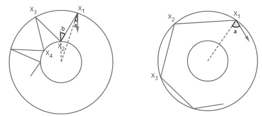
Figure 1. $\mathcal{C}_{2}$ and $\mathcal{C}_{3}$.

When considering the difference between two trajectories, we will divide the difference into singular part and nonsingular parts. In this step, we need to define shifted position and velocity, respectively.

Lemma 1.10.

Let $U:=\{(x_{1},x_{2})\in\mathbb{R}^{2}:r<x^{2}_{1}+x^{2}_{2}<R\}$. For given $p,q\in U$and $v\in\mathbb{R}^{2}$, we let

$$\tilde{p}=p+((q-p)\cdot\hat{v})\hat{v}\quad\text{and}\quad\tilde{q}=q+((p-q)\cdot\hat{v})\hat{v},$$

and assume that $|p-q|<R-r$. Then it holds that $\tilde{p}\in U$ or $\tilde{q}\in U$.

Proof.

Let $O_{r}:=\{(x_{1},x_{2})\in\mathbb{R}^{2}:x^{2}_{1}+x^{2}_{2}\leq r\}$ and $O^{c}_{R}:=\{(x_{1},x_{2})\in\mathbb{R}^{2}:x^{2}_{1}+x^{2}_{2}\geq R\}$. We fix $p,q\in U$. If $\tilde{p},\tilde{q}\in O_{r}$ or $\tilde{p},\tilde{q}\in O^{c}_{R}$, then $p\notin U$ or $q\notin U$. Moreover, if $\tilde{p}\in O^{c}_{R},\tilde{q}\in O_{r}$ or $\tilde{p}\in O_{r},\tilde{q}\in O^{c}_{R}$, then $|\tilde{p}-\tilde{q}|=|p-q|\geq R-r$. It is a contradiction, and we conclude $\tilde{p}\in U$ or $\tilde{q}\in U$.
∎

Definition 1.11.

We define shifted position $\tilde{x}(x,\bar{x},v)$ and velocity $\tilde{v}=\tilde{v}(v,\bar{v},\zeta),$ respectively.
(i) Fix $x,\bar{x}\in\Omega,v\in\mathbb{R}^{3}$, where $|x-\bar{x}|\leq 1$. Let us assume

$$x_{p}-\bar{x}_{p}\neq 0 v_{p}\neq 0 (x_{p}-\bar{x}_{p})\cdot v_{p}\neq\pm|x_{p}-\bar{x}_{p}||v|_{p}$$ is neither parallel nor anti-parallel to , i.e., .
(1.32)

In this case, we define shifted $\tilde{x}$ as

$$\tilde{x}_{p}=\tilde{x}(x,\bar{x},v)_{p}:=\bar{x}_{p}+\big{(}(x_{p}-\bar{x}_{p})\cdot\frac{v_{p}}{|v|_{p}}\big{)}\frac{v_{p}}{|v|_{p}},\quad\tilde{x}_{ver}=x_{ver}.$$ (1.33)

We define

$$\mathbf{x}(\tau)=\mathbf{x}(\tau;x,\bar{x},v):=(1-\tau){\tilde{x}}+\tau x,\quad\dot{\mathbf{x}}(\tau)=x_{p}-\tilde{x}_{p},$$ (1.34)

and $\mathbf{x}(0)=\tilde{x},\;\mathbf{x}(1)=x.$ If $\tilde{x}(x,\bar{x},v)$ is not in $\Omega$, we rename $x$ as $\bar{x}$, and $\bar{x}$ as $x$. Then there exists $\tilde{x}(x,\bar{x},v)\in\Omega$ by Lemma 1.10.
(ii) For fixed $v,\bar{v},\zeta$, let us assume

$$(v+\zeta)_{p}\neq 0 (\bar{v}+\zeta)_{p}\neq 0$$ is neither parallel nor anti-parallel to , (1.35)

i.e., $(v+\zeta)_{p}\cdot(\bar{v}+\zeta)_{p}\neq\pm|v+\zeta|_{p}||\bar{v}+\zeta|_{p}.$ In this case, we define shifted $\tilde{v}$ as

$$(\tilde{v}+\zeta)_{p}=(\tilde{v}(v,\bar{v},\zeta)+\zeta)_{p}:=|v+\zeta|_{p}\frac{(\bar{v}+\zeta)_{p}}{|\bar{v}+\zeta|_{p}},\quad(\tilde{v}+\zeta)_{ver}:=(v+\zeta)_{ver}.$$ (1.36)

We define

$$\mathbf{v}(\tau)=\mathbf{v}(\tau;x,v,\bar{v},\zeta):=|v+\zeta|_{p}R_{(v,\bar{v},\zeta)}\begin{bmatrix}\cos\Theta(\tau)\\ \sin\Theta(\tau)\\ 0\end{bmatrix}+(v+\zeta)_{ver},$$ (1.37)

$$\Theta(\tau):=\tau\theta,\quad\dot{\Theta}(\tau)=\dot{\Theta}:=\theta,$$

where $\theta=\cos^{-1}(\widehat{(v+\zeta)_{p}},\widehat{(\bar{v}+\zeta)_{p}})\in[0,2\pi)$ is the angle between $(v+\zeta)_{p}$ and $(\bar{v}+\zeta)_{p}$, and

$$R_{(v,\bar{v},\zeta)}:=\begin{bmatrix}&&\\ \widehat{(\bar{v}+\zeta)_{p}}&\widehat{(v+\zeta)_{p}}&\widehat{(\bar{v}+\zeta)_{p}}\times\widehat{(v+\zeta)_{p}}\\ &&\\ \end{bmatrix}\begin{bmatrix}1&\cos\theta&0\\ 0&\sin\theta&0\\ 0&0&1\end{bmatrix}^{-1},$$

at

$$\Theta(0)=0,\;\Theta(1)=\theta\quad\text{and}\quad\mathbf{v}(0)=\tilde{v}+\zeta,\;\mathbf{v}(1)=v+\zeta.$$

To define (1.33), we assume that $|x-\bar{x}|<R-r$, and this assumption is derived from Lemma 1.10. For convenience, we assume that $R-r>1$ in Definition 1.1.

Now, we consider $\tilde{x}\in\Omega$ and $v\in\mathbb{R}^{3}$ which satisfy $\tilde{x}(x,\tilde{x},v)=\tilde{x}$ and $\tilde{v}(v,\tilde{v},\zeta)=\tilde{v}$ in (1.33), (1.36) for given $x\in\Omega$ and $v,\zeta\in\mathbb{R}^{3}$. We define the sets A and B, which consist of elements $(x,\tilde{x},v)$, where $(\mathbf{x}(\tau),v)\in\mathcal{C}_{1}$ for all $\tau\in[0,1]$ and $(\mathbf{x}(\tau),v)\in\mathcal{C}_{2}$ for all $\tau\in[0,1]$, respectively. Here, A and B do not include all $(x,\tilde{x},v)\in\Omega\times\Omega\times\mathbb{R}^{3}$. Next, we define the important quantities $\mathfrak{S}_{sp}(\tau;x,\tilde{x},v)$ and $\mathfrak{S}_{vel}(\tau;x,v,\tilde{v},\zeta)$, which are used in section 3.

Definition 1.12.

For $\mathbf{x}(\tau)$ in (1.34), we define $A:=\{(x,\tilde{x},v):(\mathbf{x}(\tau),v)\in\mathcal{C}_{1}$ for all $\tau\in[0,1]\}$ and $B:=\{(x,\tilde{x},v):(\mathbf{x}(\tau),v)\in\mathcal{C}_{2}$ for all $\tau\in[0,1]$}. We recall (1.24), and define

$$\frac{1}{\mathfrak{S}^{1}_{sp}(\tau;x,\tilde{x},v)}:= \Big{|}\frac{X_{0}(\mathbf{x}(\tau),v)_{p}\cdot\frac{\dot{\mathbf{x}}(\tau)}{|\dot{\mathbf{x}}(\tau)|}}{X_{0}(\mathbf{x}(\tau),v)_{p}\cdot v}\Big{|}\mathbf{1}_{A}+\Big{|}\frac{X_{1}(\mathbf{x}(\tau),v)_{p}\cdot\frac{\dot{\mathbf{x}}(\tau)}{|\dot{\mathbf{x}}(\tau)|}}{X_{1}(\mathbf{x}(\tau),v)_{p}\cdot v}\Big{|}\mathbf{1}_{B},$$

$$\frac{1}{\mathfrak{S}^{2}_{sp}(\tau;x,\tilde{x},v)}:= \Big{|}\frac{X_{1}(\mathbf{x}(\tau),v)_{p}\cdot\frac{\dot{\mathbf{x}}(\tau)}{|\dot{\mathbf{x}}(\tau)|}}{X_{1}(\mathbf{x}(\tau),v)_{p}\cdot v}\Big{|}\mathbf{1}_{A}+\Big{|}\frac{X_{0}(\mathbf{x}(\tau),v)_{p}\cdot\frac{\dot{\mathbf{x}}(\tau)}{|\dot{\mathbf{x}}(\tau)|}}{X_{0}(\mathbf{x}(\tau),v)_{p}\cdot v}\Big{|}\mathbf{1}_{B},$$

and

$$\frac{1}{\mathfrak{S}_{sp}(\tau;x,\tilde{x},v)}:=\frac{1}{\mathfrak{S}^{1}_{sp}(\tau;x,\tilde{x},v)}+\frac{1}{\mathfrak{S}^{2}_{sp}(\tau;x,\tilde{x},v)}.$$

For $\mathbf{v}(\tau)$ in (1.37), we define $D:=\{(x,\tilde{x},v):(x,\mathbf{v}(\tau))\in\mathcal{C}_{1}$ for all $\tau\in[0,1]\}$ and $E:=\{(x,\tilde{x},v):(x,\mathbf{v}(\tau))\in\mathcal{C}_{2}$ for all $\tau\in[0,1]\}$. We recall (1.21), (1.22), and define

$$\frac{1}{\mathfrak{S}_{vel}^{1}(\tau;x,v,\tilde{v},\zeta)} :=t_{f}(x,\mathbf{v}(\tau))\Big{|}\frac{X_{0}(x,\mathbf{v}(\tau))_{p}\cdot\frac{\dot{\mathbf{v}}(\tau)}{|\dot{\mathbf{v}}(\tau)|}}{X_{0}(x,\mathbf{v}(\tau))_{p}\cdot\mathbf{v}(\tau)}\Big{|}\mathbf{1}_{D}+t_{b}(x,\mathbf{v}(\tau))\Big{|}\frac{X_{1}(x,\mathbf{v}(\tau))_{p}\cdot\frac{\dot{\mathbf{v}}(\tau)}{|\dot{\mathbf{v}}(\tau)|}}{X_{1}(x,\mathbf{v}(\tau))_{p}\cdot\mathbf{v}(\tau)}\Big{|}\mathbf{1}_{E},$$

$$\frac{1}{\mathfrak{S}_{vel}^{2}(\tau;x,v,\tilde{v},\zeta)} :=t_{b}(x,\mathbf{v}(\tau))\Big{|}\frac{X_{1}(x,\mathbf{v}(\tau))_{p}\cdot\frac{\dot{\mathbf{v}}(\tau)}{|\dot{\mathbf{v}}(\tau)|}}{X_{1}(x,\mathbf{v}(\tau))_{p}\cdot\mathbf{v}(\tau)}\Big{|}\mathbf{1}_{D}+t_{f}(x,\mathbf{v}(\tau))\Big{|}\frac{X_{0}(x,\mathbf{v}(\tau))_{p}\cdot\frac{\dot{\mathbf{v}}(\tau)}{|\dot{\mathbf{v}}(\tau)|}}{X_{0}(x,\mathbf{v}(\tau))_{p}\cdot\mathbf{v}(\tau)}\Big{|}\mathbf{1}_{E},$$

and

$$\frac{1}{\mathfrak{S}_{vel}(\tau;x,v,\tilde{v},\zeta)}:=\frac{1}{\mathfrak{S}_{vel}^{1}(\tau;x,v,\tilde{v},\zeta)}+\frac{1}{\mathfrak{S}_{vel}^{2}(\tau;x,v,\tilde{v},\zeta)}.$$

In section 5, we estimate the seminorms below, which are used in the proof of Theorem 1.3.

Definition 1.13 (seminorms).

Let $x,\bar{x}\in\Omega$ and $v,\bar{v},\zeta\in\mathbb{R}^{3}$. For $\varpi>0$, we define

$$\begin{split}\mathfrak{H}^{2\beta}_{sp}(s)&:=\sup_{\begin{subarray}{c}x\in{\Omega},\\ 0<|v-\bar{v}|\leq 1\end{subarray}}e^{-\varpi\langle v\rangle^{2}s}\int_{\zeta}k_{c}(v,v+\zeta)\frac{|f(s,x,v+\zeta)-f(s,\bar{x},v+\zeta)|}{|x-\bar{x}|^{2\beta}}d\zeta,\\ \end{split}$$

$$\begin{split}\mathfrak{H}^{2\beta}_{vel}(s)&:=\sup_{\begin{subarray}{c}v\in\mathbb{R}^{3},\\ 0<|x-\bar{x}|\leq 1\end{subarray}}e^{-\varpi\langle v\rangle^{2}s}\int_{\zeta}\mathbf{k}_{c}(v,\bar{v},\zeta)\frac{|f(s,x,v+\zeta)-f(s,x,\bar{v}+\zeta)|}{|v-\bar{v}|^{2\beta}}d\zeta,\\ \end{split}$$

where $\langle v\rangle:=\sqrt{1+|v|^{2}}$.

1.3. Scheme of Proof and Organization of the Paper

1.3.1. Nonlocal to local iteration scheme

We provide a brief overview of each section. We rewrite

$$\partial_{t}f+v\cdot\nabla_{x}f=\Gamma_{\text{gain}}(f,f)-\nu(f)f,\ \ f|_{t=0}=f_{0},\ \ f(t,x,v)|_{\partial\Omega}=f(t,x,R_{x}v).$$ (1.38)

and

$$\begin{split}f(t,x,v)&=e^{-\int^{t}_{0}\nu(f)(\tau,X(\tau;t,x,v),V(\tau;t,x,v))d\tau}f(0,X(0;t,x,v),V(0;t,x,v))\\ &\ \ +\int^{t}_{0}e^{-\int^{t}_{s}\nu(f)(\tau,X(\tau;t,x,v),V(\tau;t,x,v))d\tau}\Gamma_{\text{gain}}(f,f)(s,X(s;t,x,v),V(s;t,x,v))ds.\end{split}$$ (1.39)

Using (1.39) and a version of Carleman’s representation and a priori $L^{\infty}$-bound of $f$, we can derive the difference quotients for $\beta$,

$$\begin{split}&\frac{|f(t,x,v+\zeta)-f(t,\bar{x},\bar{v}+\zeta)|}{|(x,v)-(\bar{x},\bar{v})|^{\beta}}\\ &\lesssim\int_{0}^{t}\frac{|X(s)-\bar{X}(s)|^{2\beta}}{|(x,v)-(\bar{x},\bar{v})|^{\beta}}J_{x}[f(s)](V(s);X(s),\bar{X}(s))ds\\ &\quad+\int_{0}^{t}\frac{|V(s)-\bar{V}(s)|^{2\beta}}{|(x,v)-(\bar{x},\bar{v})|^{\beta}}J_{v}[f(s)](X(s);V(s),\bar{V}(s))ds+good\ terms\\ &\lesssim\sup_{s,v,x\neq\bar{x}}J_{x}[f(s)](v;x,\bar{x})\times\int_{0}^{t}\frac{|X(s)-\bar{X}(s)|^{2\beta}}{|(x,v)-(\bar{x},\bar{v})|^{\beta}}ds\\ &\quad+\sup_{s,x,v\neq\bar{v}}J_{v}[f(s)](x;v,\bar{v})\times\int_{0}^{t}\frac{|V(s)-\bar{V}(s)|^{2\beta}}{|(x,v)-(\bar{x},\bar{v})|^{\beta}}ds+good\ terms,\end{split}$$ (1.40)

where $\mathbf{J}$-seminorms are defined as

$$\begin{split}J_{x}[f(s)](V(s);X(s),\bar{X}(s))&:=\int_{|u|\lesssim 1}\frac{|f(s,X(s),u+V(s))-f(s,\bar{X}(s),u+V(s))|}{|X(s)-\bar{X}(s)|^{2\beta}}du,\\ J_{v}[f(s)](X(s);V(s),\bar{V}(s))&:=\int_{|u|\lesssim 1}\frac{|f(s,X(s),u+V(s))-f(s,X(s),u+\bar{V}(s))|}{|V(s)-\bar{V}(s)|^{2\beta}}du.\end{split}$$ (1.41)

Note that $X(s)=X(s;t,x,v+\zeta)$, $V(s)=V(s;t,x,v+\zeta)$, $\bar{X}(s)=\bar{X}(s;t,\bar{x},\bar{v}+\zeta)$, and $\bar{V}(s)=\bar{V}(s;t,\bar{x},\bar{v}+\zeta)$. From the Duhamel form of (1.39), we obtain the inequality about the $\mathbf{J}$-seminorms (1.41) as

$$\begin{split}J_{x}[f(s)](v;x,\bar{x})&\lesssim\ \int^{t}_{0}\int_{|\zeta|\leq 1}\frac{|X(s)-\bar{X}(s)|^{2\beta}}{|x-\bar{x}|^{2\beta}}d\zeta ds\times\sup_{s,v,x\neq\bar{x}}J_{x}[f(s)](v;x,\bar{x})\\ &\quad+\int^{t}_{0}\int_{|\zeta|\leq 1}\frac{|V(s)-\bar{V}(s)|^{2\beta}}{|x-\bar{x}|^{2\beta}}d\zeta ds\times\sup_{s,x,v\neq\bar{v}}J_{v}[f(s)](x;v,\bar{v})+good\ terms\\ &\lesssim\sup_{\begin{subarray}{c}v\in\mathbb{R}^{3}\\ 0<|x-\bar{x}|\leq 1\end{subarray}}\langle v\rangle\frac{|f_{0}(x,v)-f_{0}(\bar{x},v)|}{|x-\bar{x}|^{2\beta}}+\sup_{\begin{subarray}{c}x\in\bar{\Omega}\\ 0<|v-\bar{v}|\leq 1\end{subarray}}\langle v\rangle^{2}\frac{|f_{0}(x,v)-f_{0}(x,\bar{v})|}{|v-\bar{v}|^{2\beta}}+\|w_{0}f_{0}\|_{\infty}\\ &\quad+\frac{1}{\varpi}\Big{[}\sup_{s,v,x\neq\bar{x}}J_{x}[f(s)](v;x,\bar{x})+\sup_{s,x,v\neq\bar{v}}J_{v}[f(s)](x;v,\bar{v})\Big{]}\mathcal{P}_{3}(\|e^{\vartheta_{0}|v|^{2}}f_{0}\|_{\infty})\end{split}$$ (1.42)

for $0<\beta<1/4$, and we also have a similar expression for $J_{v}[f(s)](x;v,\bar{v})$. The key is to calculate the integral of the fractional trajectory in (1.42). Then we obtain the uniform bound of $J_{x}[f(s)](v;x,\bar{x})$ and $J_{v}[f(s)](x;v,\bar{v})$ for sufficiently large $\varpi\gg_{f_{0},\beta}1$. Next, we use (1.40) to bound the Hölder seminorm.

Now, we briefly outline each section. In section 1, we obtain the explicit formula $(X(s;t,x,v),V(s;t,x,v))$. To get the uniform bound of $J_{x}[f(s)](v;x,\bar{x})$ and $J_{v}[f(s)](x;v,\bar{v})$ from (1.42), we estimate

$$|(X,V)(s;t,x,v)-(X,V)(s;t,\bar{x},\bar{v})|/|(x,v)-(\bar{x},\bar{v})|$$

for $x,\bar{x}\in\Omega$, $v,\bar{v}\in\mathbb{R}^{3}$ in section 3,4, and we perform the integral estimate in section 5. Moreover, in section 6, we estimate

$$|(X,V)(s;t,x,v)-(X,V)(s;t,\bar{x},\bar{v})|/|(x,v)-(\bar{x},\bar{v})|^{1/2},$$

and refer to these results as $C^{0,\frac{1}{2}}_{x,v}$ estimates of trajectory. Lastly, we apply the uniform bound of $J_{x}[f(s)](v;x,\bar{x})$, $J_{v}[f(s)](x;v,\bar{v})$ and $C^{0,\frac{1}{2}}_{x,v}$ estimates of trajectory to (1.40), and prove the Theorem 1.3 in section 7.

1.3.2. The results of each section

We summarize the results for each section in more detail. The particle’s trajectory exhibits a repetitive pattern in the cylindrical annulus domain. Therefore, in section 2, we can formulate the trajectories satisfying the specular condition into three cases. We classify the case where the first backward in time bouncing point is on the inner circle as $\mathcal{C}_{1}$, and on the outer circle as $\mathcal{C}_{2}$. We also classify $\mathcal{C}_{3}$ as the situation where the particle exclusively hits the outer circle. (See Figure 1.) For the particle that has velocity $v$ at space $x$, $a(x,v)$ is the angle between the normal vector at the point of collision and the velocity when the particle hits the outer circle, and $b(x,v)$ is the angle when the particle hits the inner circle. We derive

$$\cos a(x,v)=\sqrt{1-|x|_{p}^{2}/R^{2}+(x_{p}\cdot\hat{v}_{p})^{2}/R^{2}}>0,$$ (1.43)

$$\cos b(x,v)=\sqrt{1-|x|_{p}^{2}/r^{2}+(x_{p}\cdot\hat{v}_{p})^{2}/r^{2}}\geq 0.$$

Also, $X(s;t,x,v)$ and $V(s;t,x,v)$ can be expressed in terms of $a(x,v)$ and $b(x,v)$. Let us denote grazing collision when a particle grazes an inner circle. In the case of grazing collisions, the trajectory can be expressed as either $\mathcal{C}_{1}$ or $\mathcal{C}_{2}$, and it can be also expressed as $\mathcal{C}_{3}$ in Remark 2.8.

In section 3, we consider a trajectory that belongs to $\mathcal{C}_{1}$ or $\mathcal{C}_{2}$. Given $x,\bar{x}\in\Omega$, $v,\bar{v}\in\mathbb{R}^{3}$, we assume that $(\mathbf{x}(\tau),v),(x,\mathbf{v}(\tau))\in\mathcal{C}_{1}$ for all $\tau\in[0,1]$ or $(\mathbf{x}(\tau),v),(x,\mathbf{v}(\tau))\in\mathcal{C}_{2}$ for all $\tau\in[0,1]$. Using the difference between trajectories, we obtain

$$\begin{split}|(X,V)(s;t,x,v)-(X,V)(s;t,\bar{x},v)|/|x-\bar{x}|\lesssim_{|v|}\int_{0}^{1}\frac{1}{\mathfrak{S}_{sp}(\tau;x,\tilde{x},v)}\;d\tau\end{split}$$ (1.44)

and

$$\begin{split}|(X,V)(s;t,x,v)-(X,V)(s;t,x,\bar{v})|/|v-\bar{v}|\lesssim_{|v|}\int_{0}^{1}\frac{1}{\mathfrak{S}_{vel}(\tau;x,v,\tilde{v},\zeta)}\;d\tau\end{split}$$ (1.45)

for $x,\bar{x}\in\Omega$, $v,\bar{v}\in\mathbb{R}^{3}$. We note that the above results are equivalent to the case where a particle hits once outside of a general convex domain. If $(x,v)\notin\mathcal{G}$, $(\tilde{x},v)\in\mathcal{G}$, we obtain

$$\int_{0}^{1}\frac{1}{\mathfrak{S}_{sp}(\tau;x,\tilde{x},v)}\;d\tau\lesssim_{|v|}\frac{1}{\cos b(x,v)}$$

by singularity averaging in Lemma 3.8. Also, if $(x,v+\zeta)\notin\mathcal{G}$, $(x,\tilde{v}+\zeta)\in\mathcal{G}$, we obtain

$$\int_{0}^{1}\frac{1}{\mathfrak{S}_{vel}(\tau;x,v,\tilde{v},\zeta)}\;d\tau\lesssim_{|v|}\frac{1}{\cos b(x,v+\zeta)}$$

by singularity averaging in Lemma 3.10.

In section 4, we consider $\mathcal{C}_{3}$ case. Given $x,\bar{x}\in\Omega$, $v,\bar{v}\in\mathbb{R}^{3}$, we assume that $(\mathbf{x}(\tau),v),(x,\mathbf{v}(\tau))\in\mathcal{C}_{3}$ for all $\tau\in[0,1]$. Then,

$$\begin{split}&|X(s;t,x,v)-X(s;t,\bar{x},v)|/|x-\bar{x}|\lesssim_{|v|}\text{max}\{\frac{1}{\cos a(x,v)},\frac{1}{\cos a(\bar{x},v)}\},\end{split}$$ (1.46)

$$\begin{split}&|V(s;t,x,v)-V(s;t,\bar{x},v)|/|x-\bar{x}|\lesssim_{|v|}\text{max}\{\frac{1}{\cos^{2}a(x,v)},\frac{1}{\cos^{2}a(\bar{x},v)}\},\end{split}$$ (1.47)

and

$$\begin{split}&|X(s;t,x,v)-X(s;t,x,\bar{v})|/|v-\bar{v}|\lesssim_{|v|}1,\end{split}$$ (1.48)

$$\begin{split}&|V(s;t,x,v)-V(s;t,x,\bar{v})|/|v-\bar{v}|\lesssim_{|v|}\text{max}\{\frac{1}{\cos a(x,v)},\frac{1}{\cos a(x,\bar{v})}\}\end{split}$$ (1.49)

for $x,\bar{x}\in\Omega$, $v,\bar{v}\in\mathbb{R}^{3}$. For convex only cases $\mathcal{C}_{3}$, we can adopt the sharp result of [33] to (1.46), (1.47), and (1.48). To get (1.49), we use the difference between trajectories.

In section 5, we get estimates for the differences $|(X,V)(s;t,x,v)-(X,V)(s;t,\bar{x},\bar{v})|/|(x,v)-(\bar{x},\bar{v})|$ for $x,\bar{x}\in\Omega$, $v,\bar{v}\in\mathbb{R}^{3}$ regardless of the cases $\mathcal{C}_{1,2,3}$. Next, we obtain

$$\int\frac{e^{-c|\zeta|^{2}}}{|\zeta|}\frac{\langle v+\zeta\rangle^{r}}{|\cos b(x,v+\zeta)|^{2\beta}}\mathbf{1}_{\{(x,v+\zeta)|{(x,v+\zeta)}\in\text{$\mathcal{C}_{1,2}$}\}}\;d\zeta\lesssim_{\beta}\langle v\rangle^{r+1}$$ (1.50)

for $0<\beta<1/2$ and

$$\int\frac{e^{-c|\zeta|^{2}}}{|\zeta|}\frac{\langle v+\zeta\rangle^{r}}{|\cos a(x,v+\zeta)|^{4\beta}}\mathbf{1}_{\{(x,v+\zeta)|{(x,v+\zeta)}\in\text{$\mathcal{C}_{3}$}\}}\;d\zeta\lesssim_{\beta}\langle v\rangle^{r+1}.$$ (1.51)

for $0<\beta<1/4$. The exact definitions of the $\mathbf{J}$-seminorms, $\mathfrak{H}_{sp,vel}^{2\beta}$ are defined in Definition 1.13, and we estimate the seminorms $\mathfrak{H}_{sp,vel}^{2\beta}$ for $0<\beta<1/4$ by using (1.50), (1.51). In particular, we should take the singular order of the RHS of (1.47) into account since it is the most singular order among all fraction estimates of characteristics. We note that the range of $\beta\in(0,\frac{1}{4})$ comes from the singular order of $\cos a(x,v)$ in (1.47).

In section 6, we consider optimal $C^{0,\frac{1}{2}}_{x,v}$ regularity of trajectories in the domain. Let fix $x,\bar{x}\in\Omega$, $v,\bar{v}\in\mathbb{R}^{3}$. For $(x,v),(\bar{x},v),(x,\bar{v})\in\mathcal{C}_{1}$ or $(x,v),(\bar{x},v),(x,\bar{v})\in\mathcal{C}_{2}$, we obtain

$$|(X,V)(s;t,x,v)-(X,V)(s;t,\bar{x},\bar{v})|/|(x,v)-(\bar{x},\bar{v})|^{1/2}\lesssim_{|v|}1.$$

For $(x,v),(\bar{x},v),(x,\bar{v})\in\mathcal{C}_{3}$, we obtain

$$\begin{split}&|(X,V)(s;t,x,v)-(X,V)(s;t,\bar{x},v)|/|x-\bar{x}|^{1/2}\lesssim_{|v|}\text{min}\{\frac{1}{\cos a(x,v)},\frac{1}{\cos a(\bar{x},v)}\}\end{split}$$ (1.52)

and

$$\begin{split}&|V(s;t,x,v)-V(s;t,x,\bar{v})|/|v-\bar{v}|^{1/2}\lesssim_{|v|}\text{max}\{\frac{1}{\cos^{1/2}a(x,v)},\frac{1}{\cos^{1/2}a(x,\bar{v})}\}.\end{split}$$ (1.53)

Therefore, if the order of $|(x,v)-(\bar{x},\bar{v})|$ is reduced by 1/2, then the order of singularity of (1.44), (1.45), and (1.47) decrease by 1, and (1.49) decreases by $1/2$. Moreover, the maximum value of cosines in (1.46), (1.47) is replaced by the minimum value of cosines.

In the last section 7, we prove (1.12) in Theorem 1.3 combining $C^{0,\frac{1}{2}}_{x,v}$ estimates of trajectory and $\mathfrak{H}_{sp,vel}^{2\beta}$ estimates. Due to the singularity of $C^{0,\frac{1}{2}}_{x,v}$ estimates of trajectory in (1.52), (1.53), there are the singularity of the form of $\cos b(x,v)$ on RHS of the inequality, (1.40). Since the singularity can be expressed by (1.43), the weight $h(y,w)$ in (1.10) is multiplied by the Hölder norm in (1.12).

2. Trajectory analysis

Lemma 2.1.

Suppose the domain is given as in Definition 1.1. For $(x,v)\in\Omega\times\mathbb{R}^{3}$ and $k\in\mathbb{N}\cup\{0\}$, we let

$$V_{k+1}(x,v)=V_{k}(x,v)-2(n(X_{k+1}(x,v))\cdot V_{k}(x,v))n(X_{k+1}(x,v)),$$ (2.1)

$$t_{b,k+1}(x,v)=t_{b}(X_{k+1}(x,v),V_{k+1}(x,v)),\quad t_{b,0}(x,v)=t_{b}(X_{0}(x,v),V_{0}(x,v))=t_{*}(x,v),$$

$$X_{k+2}(x,v)=X_{k+1}(x,v)-t_{b,k+1}(x,v)V_{k+1}(x,v),$$ (2.2)

where $t_{*}(x,v)$ is defined in (1.23). Then it holds that

$$t_{b,k+1}(x,v)=t_{*}(x,v),\quad|X_{2k}(x,v)|_{p}=|X_{0}(x,v)|_{p},\quad|X_{2k+1}(x,v)|_{p}=|X_{1}(x,v)|_{p},$$ (2.3)

and

$$\begin{split}&n(X_{2k}(x,v))\cdot V_{2k}(x,v)=n(X_{0}(x,v))\cdot V_{0}(x,v),\\ &n(X_{2k+1}(x,v))\cdot V_{2k+1}(x,v)=n(X_{1}(x,v))\cdot V_{1}(x,v).\end{split}$$ (2.4)

Proof.

Taking the inner product of $n(X_{k+1}(x,v))$ to (2.1),

$$X_{k+1}(x,v)_{p}\cdot V_{k+1}(x,v)=-X_{k+1}(x,v)_{p}\cdot V_{k}(x,v).$$ (2.5)

Using $\eqref{inner}$ and $|V_{k}(x,v)|_{p}=|V_{k+1}(x,v)|_{p}$, we get

$$|X_{k+1}(x,v)+\tau V_{k}(x,v)|_{p}^{2}=|X_{k+1}(x,v)-\tau V_{k+1}(x,v)|_{p}^{2}.$$ (2.6)

For $t_{b}(x,v)$ in (1.21),

$$t_{b,k+1}(x,v) =t_{b}{(X_{k+1}(x,v),V_{k+1}(x,v))}$$

$$=\sup\big{\{}s\geq 0:X_{k+1}(x,v)-\tau V_{k+1}(x,v)\in\Omega\ \ \text{for all}\ \tau\in(0,s)\big{\}}$$

$$=\sup\big{\{}s\geq 0:r<|X_{k+1}(x,v)-\tau V_{k+1}(x,v)|_{p}<R\ \ \text{for all}\ \tau\in(0,s)\big{\}}$$

$$=\sup\big{\{}s\geq 0:r<|X_{k+1}(x,v)+\tau V_{k}(x,v)|_{p}<R\ \ \text{for all}\ \tau\in(0,s)\big{\}}$$

$$=t_{b}(X_{k+1}(x,v),-V_{k}(x,v))=t_{b}(X_{k}(x,v),V_{k}(x,v))=t_{b,k}(x,v).$$

Then, $t_{b,k}(x,v)=t_{b,k-1}(x,v)\cdots=t_{b,0}(x,v)=t_{*}(x,v).$ From (2.2),

$$X_{k}(x,v)=X_{k+1}(x,v)+t_{*}(x,v)V_{k}(x,v), X_{k+2}(x,v)=X_{k+1}(x,v)-t_{*}(x,v)V_{k+1}(x,v),$$

and using (2.5), we get $|X_{k+2}(x,v)|_{p}=|X_{k}(x,v)|_{p}$ by computation. By using (2.5) and (2.2),

$$n(X_{k+2}(x,v))\cdot V_{k+2}(x,v) =-n(X_{k+2}(x,v))\cdot V_{k+1}(x,v)$$

$$=({-n(X_{k+1}(x,v))+t_{*}(x,v)V_{k+1}(x,v)_{p}})\cdot V_{k+1}(x,v)$$

$$=-n(X_{k+1}(x,v))\cdot V_{k+1}(x,v)+t_{*}(x,v)|v|_{p}^{2}$$

$$=n(X_{k}(x,v))\cdot V_{k}(x,v)+(t_{*}(x,v)-t_{*}(x,v))|v|_{p}^{2}$$

$$=n(X_{k}(x,v))\cdot V_{k}(x,v).$$

For $k\in\mathbb{N}\cup\{0\}$, we conclude

$$|X_{2k}(x,v)|_{p}=|X_{0}(x,v)|_{p},\quad|X_{2k+1}(x,v)|_{p}=|X_{1}(x,v)|_{p},$$

and

$$n(X_{2k}(x,v))\cdot V_{2k}(x,v)=n(X_{0}(x,v))\cdot V_{0}(x,v),$$

$$n(X_{2k+1}(x,v))\cdot V_{2k+1}(x,v)=n(X_{1}(x,v))\cdot V_{1}(x,v).$$

∎

Definition 2.2.

We define

$$m(s;t,x,v):=[(t-t_{b}(x,v)-s)/t_{*}(x,v)]+1\in\mathbb{N}\cup\{0\}$$ (2.7)

and

$$t_{k}(t,x,v):=t-t_{b}(x,v)-(k-1)t_{*}(x,v)$$ (2.8)

for $k\in[0,m(0;t,x,v)]$. We define

$$X(s;t,x,v):=X_{k}(x,v)-V_{k}(x,v)(t_{k}(t,x,v)-s),$$

$$V(s;t,x,v):=V_{k}(x,v),$$

where (2.1), (2.2), and $k=m(s;t,x,v)$.

Remark 2.3 (orientation).

Given $(x,v)\in\Omega\times\mathbb{R}^{3}$, let us $x=(|x|_{p}\cos\theta_{x},|x|_{p}\sin\theta_{x},x_{3}),$
$v=(|v|_{p}\cos\theta_{v},|v|_{p}\sin\theta_{v},v_{3})$ for $\theta_{x},\theta_{v}\in[-\pi,\pi]$. If $0<\theta_{x}-\theta_{v}<\pi$ in mod $2\pi$, then $X(s;t,x,v)$ moves clockwise. If $-\pi<\theta_{x}-\theta_{v}<0$ in mod $2\pi$, then $X(s;t,x,v)$ moves counter-clockwise. If $\theta_{x}-\theta_{v}=0$ or $\pi$, then $X(s;t,x,v)$ moves repeatedly between some two points. In this paper, we assume that $X(s;t,x,v)$ is concluded in both moving clockwise case and moving counter-clockwise case if $\theta_{x}-\theta_{v}=0$ or $\pi$.

Lemma 2.4.

Suppose that the domain is given as in Definition 1.1.
Let $x=(|x|_{p}\cos\theta_{x},|x|_{p}\sin\theta_{x},x_{3}),\;v=(|v|_{p}\cos\theta_{v},|v|_{p}\sin\theta_{v},v_{3})$ for $\theta_{x},\theta_{v}\in[-\pi,\pi]$, and assume that $0\leq\theta_{x}-\theta_{v}\leq\pi$ in mod $2\pi$.
(1) Assume $(x,v)\in\mathcal{C}_{1}$. Then,

$$\begin{split}&a(x,v)=\sin^{-1}\Big{(}\frac{|x|_{p}}{R}\sin(\theta_{x}-\theta_{v})\Big{)}\in[0,\pi/2),\\ &b(x,v)=\sin^{-1}\Big{(}\frac{|x|_{p}}{r}\sin(\theta_{x}-\theta_{v})\Big{)}\in[0,\pi/2],\end{split}$$ (2.9)

where $a(x,v),b(x,v)$ are in (1.28).
(2) Assume $(x,v)\in\mathcal{C}_{2}$. Then we have (2.9), where $a(x,v),b(x,v)$ are in (1.29).
(3)Assume $(x,v)\in\mathcal{C}_{3}$. Then we have (2.9), where $a(x,v)$ is in (1.30).

Proof.

We assume that $(x,v)\in\mathcal{C}_{1}$ with moving clockwise, and draw the points $X_{0}(x,v)_{p}$, $X_{1}(x,v)_{p}$, $x_{p}$, and $v_{p}$ in Figure 2. By sine law,

$$\frac{|x|_{p}}{\sin a(x,v)}=\frac{R}{\sin(\theta_{x}-\theta_{v})}\quad\text{and}\quad\frac{|x|_{p}}{\sin b(x,v)}=\frac{r}{\sin(\theta_{x}-\theta_{v})},$$ (2.10)

where $a(x,v),b(x,v)$ are in (1.28), and we get (2.9). Similarly, (2.9) is true when $(x,v)\in$ $\mathcal{C}_{2}$ or $\mathcal{C}_{3}$ with moving clockwise. Therefore, we also obtain

$$\begin{split}&\cos a(x,v)=\sqrt{1-|x|_{p}^{2}/R^{2}+(x_{p}\cdot\hat{v}_{p})^{2}/R^{2}}>0,\\ &\cos b(x,v)=\sqrt{1-|x|_{p}^{2}/r^{2}+(x_{p}\cdot\hat{v}_{p})^{2}/r^{2}}\geq 0\end{split}$$ (2.11)

from (2.9). ∎

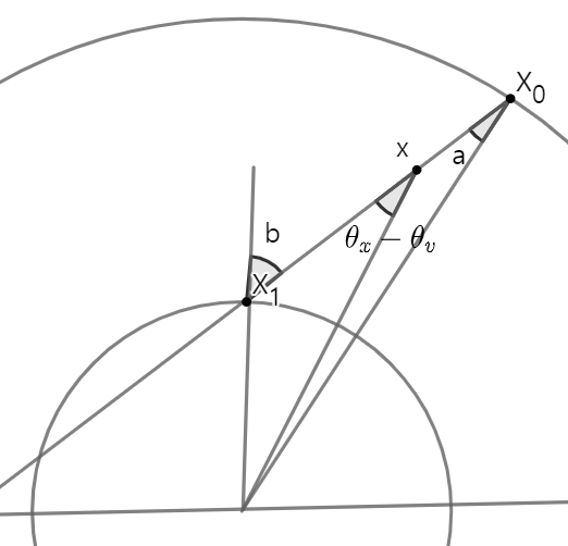
Figure 2. the relationship between angles.

Remark 2.5.

Let $x=(|x|_{p}\cos\theta_{x},|x|_{p}\sin\theta_{x},x_{3}),\;v=(|v|_{p}\cos\theta_{v},|v|_{p}\sin\theta_{v},v_{3})$ for $\theta_{x},\theta_{v}\in[-\pi,\pi]$, and assume that $-\pi\leq\theta_{x}-\theta_{v}\leq 0$ in mod $2\pi$. Then we have $a(x,v)=\sin^{-1}(-\frac{|x|_{p}}{R}\sin(\theta_{x}-\theta_{v}))$ and $b(x,v)=\sin^{-1}(-\frac{|x|_{p}}{r}\sin(\theta_{x}-\theta_{v}))$.

Lemma 2.6.

Suppose that the domain is given as in Definition 1.1.
Let $x=(|x|_{p}\cos\theta_{x},|x|_{p}\sin\theta_{x},x_{3}),\;v=(|v|_{p}\cos\theta_{v},|v|_{p}\sin\theta_{v},v_{3})$ for $\theta_{x},\theta_{v}\in[-\pi,\pi]$. We assume $0\leq\theta_{x}-\theta_{v}\leq\pi$ in mod $2\pi$.
(1) Assume $(x,v)\in\mathcal{C}_{1}$. For $k\in\mathbb{N}\cup\{0\}$,

$$X_{2k}(x,v)=(R\cos\theta_{X_{2k}}(x,v),R\sin\theta_{X_{2k}}(x,v),x_{3}-v_{3}(t_{b}(x,v)+(2k-1)t_{*}(x,v))),$$

$$X_{2k+1}(x,v)=(r\cos\theta_{X_{2k+1}}(x,v),r\sin\theta_{X_{2k+1}}(x,v),x_{3}-v_{3}(t_{b}(x,v)+2kt_{*}(x,v))),$$ (2.12)

where

$$\theta_{X_{k}}(x,v)=\theta_{v}+kb(x,v)-(k-1)a(x,v)$$

for $a(x,v),b(x,v)$ in (1.28).
(2) Assume $(x,v)\in\mathcal{C}_{2}$. For $k\in\mathbb{N}\cup\{0\}$,

$$\begin{split}&X_{2k}(x,v)=(r\cos\theta_{X_{2k}}(x,v),r\sin\theta_{X_{2k}}(x,v),x_{3}-v_{3}(t_{b}(x,v)+(2k-1)t_{*}(x,v))),\\ &X_{2k+1}(x,v)=(R\cos\theta_{X_{2k+1}}(x,v),R\sin\theta_{X_{2k+1}}(x,v),x_{3}-v_{3}(t_{b}(x,v)+2kt_{*}(x,v))),\end{split}$$ (2.13)

where

$$\theta_{X_{k}}(x,v)=\pi+\theta_{v}+(k-1)b(x,v)-ka(x,v)$$

for $a(x,v),b(x,v)$ in (1.29).
(3) Assume $(x,v)\in\mathcal{C}_{3}$. For $k\in\mathbb{N}\cup\{0\}$,

$$X_{k}(x,v)=(R\cos\theta_{X_{k}}(x,v),R\sin\theta_{X_{k}}(x,v),x_{3}-v_{3}(t_{b}(x,v)+(k-1)t_{*}(x,v))),$$ (2.14)

where

$$\theta_{X_{k}}(x,v)=k\pi+\theta_{v}+(1-2k)a(x,v)$$

for $a(x,v)$ in (1.30).

Proof.

For $k\in\mathbb{N}\cup\{0\}$, we write

$$\begin{split}&\quad\theta_{X_{k+1}}(x,v)-\theta_{X_{k}}(x,v)\\ &=\cos^{-1}(\widehat{X_{k+1}(x,v)_{p}}\cdot\widehat{V_{k}(x,v)_{p}})-\cos^{-1}(\widehat{X_{k}(x,v)_{p}}\cdot\widehat{V_{k}(x,v)_{p}})\\ &=\cos^{-1}(-\widehat{X_{k+1}(x,v)_{p}}\cdot\widehat{V_{k+1}(x,v)_{p}})-\cos^{-1}(\widehat{X_{k}(x,v)_{p}}\cdot\widehat{V_{k}(x,v)_{p}})\end{split}$$ (2.15)

by (2.5) and $\theta_{X_{k+1}}(x,v)-\theta_{X_{k}}(x,v)\in[0,\pi/2)$.
(1) Assume $(x,v)\in\mathcal{C}_{1}$. From (1.28),

$$a(x,v)=\cos^{-1}(n(X_{0}(x,v))\cdot\widehat{V_{0}(x,v)_{p}}),\quad$$

$$b(x,v)=\cos^{-1}(n(X_{1}(x,v))\cdot\widehat{V_{0}(x,v)_{p}})=\cos^{-1}(-n(X_{1}(x,v))\cdot\widehat{V_{1}(x,v)}_{p}).$$

From (2.15),

$$\theta_{X_{k+1}}(x,v)=\theta_{X_{k}}(x,v)+b(x,v)-a(x,v),$$

$$\theta_{X_{0}}(x,v)=\theta_{v}+a(x,v).$$

We obtain $\theta_{X_{k}}(x,v)=\theta_{v}+kb(x,v)-(k-1)a(x,v)$. By using the fact $V(s;t,x,v)_{ver}=(0,0,v_{3})$ for all s and (2.3), we also obtain (2.6).

(2) Assume $(x,v)\in\mathcal{C}_{2}$. Using (1.29) and $\theta_{X_{0}}(x,v)=\theta_{v}+\pi-b(x,v)$, we obtain (2.13).

(3) Assume $(x,v)\in\mathcal{C}_{3}$. From $|X_{0}(x,v)|_{p}=|X_{1}(x,v)|_{p}=R$ and (2.3), we have $|X_{k}(x,v)|_{p}=R$. Using (2.2),

$$|X_{k+2}(x,v)|_{p}^{2}=|X_{k+1}(x,v)|_{p}^{2}-2t_{*}(x,v)X_{k+1}(x,v)_{p}\cdot V_{k+1}(x,v)+t_{*}(x,v)|v|_{p}^{2}.$$

Therefore,

$$X_{k+1}(x,v)_{p}\cdot V_{k+1}(x,v)=t_{*}(x,v)|v|_{p}^{2}$$

and the value does not depend on $k$. By $n(X_{k}(x,v))\cdot V_{k}(x,v)=n(X_{1}(x,v))\cdot V_{1}(x,v)$,

$$\cos^{-1}(-\widehat{X_{1}(x,v)_{p}}\cdot\widehat{V_{1}(x,v)_{p}})=\cos^{-1}(-\widehat{X_{0}(x,v)_{p}}\cdot\widehat{V_{0}(x,v)_{p}})=\pi-a(x,v),$$

where a(x,v) is in (1.30). We also have $\theta_{X_{0}}(x,v)=\theta_{v}+a(x,v).$ Then we have (2.14) from (2.15). ∎

Lemma 2.7.

Let $x=(|x|_{p}\cos\theta_{x},|x|_{p}\sin\theta_{x},x_{3}),\;v=(|v|_{p}\cos\theta_{v},|v|_{p}\sin\theta_{v},v_{3})$ for $\theta_{x},\theta_{v}\in[-\pi,\pi]$, and assume $0\leq\theta_{x}-\theta_{v}\leq\pi$ in mod $2\pi$.
(1) Assume $(x,v)\in\mathcal{C}_{1}$. For $k\in\mathbb{N}\cup\{0\}$,

$$\begin{split}&V_{2k}(x,v)=(|v|_{p}\cos\theta_{V_{2k}}(x,v),|v|_{p}\sin\theta_{V_{2k}}(x,v),v_{3}),\\ &V_{2k+1}(x,v)=(|v|_{p}\cos\theta_{V_{2k+1}}(x,v),|v|_{p}\sin\theta_{V_{2k+1}}(x,v),v_{3}),\end{split}$$ (2.16)

where

$$\theta_{V_{2k}}(x,v)=\theta_{v}+2k(b(x,v)-a(x,v)),$$

$$\theta_{V_{2k+1}}(x,v)=\pi+\theta_{v}+(2k+2)b(x,v)-2ka(x,v)$$

for $a(x,v),b(x,v)$ in (1.28).
(2) Assume $(x,v)\in\mathcal{C}_{2}$. For $k\in\mathbb{N}\cup\{0\}$,

$$\begin{split}&V_{2k}(x,v)=(|v|_{p}\cos\theta_{V_{2k}}(x,v),|v|_{p}\sin\theta_{V_{2k}}(x,v),v_{3}),\\ &V_{2k+1}(x,v)=(|v|_{p}\cos\theta_{V_{2k+1}}(x,v),|v|_{p}\sin\theta_{V_{2k+1}}(x,v),v_{3}),\end{split}$$ (2.17)

where

$$\theta_{V_{2k}}(x,v)=\theta_{v}+2k(b(x,v)-a(x,v)),$$

$$\theta_{V_{2k+1}}(x,v)=\pi+\theta_{v}+2kb(x,v)-(2k+2)a(x,v)$$

for $a(x,v),b(x,v)$ are in (1.29).
(3) Assume $(x,v)\in\mathcal{C}_{3}$. For $k\in\mathbb{N}\cup\{0\}$,

$$V_{k}(x,v)=(|v|_{p}\cos\theta_{V_{k}}(x,v),|v|_{p}\sin\theta_{V_{k}}(x,v),v_{3}),$$ (2.18)

where

$$\theta_{V_{k}}(x,v)=k\pi+\theta_{v}-2ka(x,v)$$

for $a(x,v)$ is in (1.30).

Proof.

For $k\in\mathbb{N}\cup\{0\}$,

$$\begin{split}\theta_{V_{k}}(x,v)&=\theta_{X_{k+1}}(x,v)-\cos^{-1}(\widehat{X_{k+1}(x,v)_{p}}\cdot\widehat{V_{k}(x,v)_{p}})\\ &=\theta_{X_{k+1}}(x,v)-\cos^{-1}(-\widehat{X_{k+1}(x,v)_{p}}\cdot\widehat{V_{k+1}(x,v)_{p}})\\ &=\theta_{X_{k+1}}(x,v)-\pi+\cos^{-1}(\widehat{X_{k+1}(x,v)_{p}}\cdot\widehat{V_{k+1}(x,v)_{p}}).\end{split}$$ (2.19)

(1) From (2.19), we get

$$\theta_{V_{2k}}(x,v)=\theta_{X_{2k+1}}(x,v)-b(x,v)=\theta_{v}+2k(b(x,v)-a(x,v)),$$

$$\theta_{V_{2k+1}}(x,v)=\theta_{X_{2k+2}}(x,v)-\pi+a(x,v)=-\pi+\theta_{v}+(2k+2)b(x,v)-2ka(x,v)$$

by (1.28), (2.4), and (2.6). By similar as in (1), we get (2.17) and (2.18). ∎

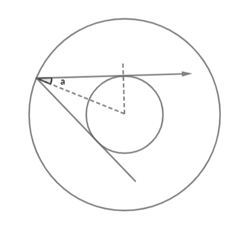
Figure 3. in the case of grazing.

Remark 2.8 (grazing).

Let $x=(|x|_{p}\cos\theta_{x},|x|_{p}\sin\theta_{x},x_{3}),\;v=(|v|_{p}\cos\theta_{v},|v|_{p}\sin\theta_{v},v_{3})$ for $\theta_{x},\theta_{v}\in[-\pi,\pi]$, and assume $0\leq\theta_{x}-\theta_{v}\leq\pi$ in mod $2\pi$. When $b(x,v)=\pi/2$ in (1.28), the trajectory can be expressed in two different ways.(See Figure 3.) One is

$$\begin{split}&X_{2k}(x,v)=(R\cos\theta_{X_{2k}}(x,v),R\sin\theta_{X_{2k}}(x,v),x_{3}-v_{3}(t_{b}(x,v)+(2k-1)t_{*}(x,v))),\\ &X_{2k+1}(x,v)=(r\cos\theta_{X_{2k+1}}(x,v),r\sin\theta_{X_{2k+1}}(x,v),x_{3}-v_{3}(t_{b}(x,v)+2kt_{*}(x,v))),\end{split}$$ (2.20)

where

$$\theta_{X_{k}}(x,v)=\theta_{v}+\frac{\pi}{2}k-(k-1)a(x,v)$$

and $a(x,v)=\sin^{-1}(r/R)\in[0,\pi/2]$. The other is

$$X_{k}(x,v)=(R\cos\theta_{X_{k}}(x,v),R\sin\theta_{X_{k}}(x,v),x_{3}-v_{3}(t_{b}(x,v)+(k-1)t_{*}(x,v))),$$ (2.21)

where

$$\theta_{X_{k}}(x,v)=k\pi+\theta_{v}+(1-2k)a(x,v)$$

and $a(x,v)=\sin^{-1}(r/R)\in[0,\pi/2]$. We can use one of the two ways depending on the situation. In this paper, we can express $(x,v)\in\mathcal{C}_{1}$ or $(x,v)\in\mathcal{C}_{3}$ when $b(x,v)=\pi/2$ in (1.28).

When $b(x,v)=\pi/2$ in (1.29),

$$\begin{split}&X_{2k}(x,v)=(r\cos\theta_{X_{2k}}(x,v),r\sin\theta_{X_{2k}}(x,v),x_{3}-v_{3}(t_{b}(x,v)+(2k-1)t_{*}(x,v))),\\ &X_{2k+1}(x,v)=(R\cos\theta_{X_{2k+1}}(x,v),R\sin\theta_{X_{2k+1}}(x,v),x_{3}-v_{3}(t_{b}(x,v)+2kt_{*}(x,v))),\end{split}$$ (2.22)

where

$$\theta_{X_{k}}(x,v)=\theta_{v}+\frac{\pi}{2}(k+1)-ka(x,v)$$

and $a(x,v)=\sin^{-1}(r/R)\in[0,\pi/2]$. Because $X(s;t,x,v)$ is also expressed by (2.21), we can write $(x,v)\in\mathcal{C}_{2}$ or $(x,v)\in\mathcal{C}_{3}$ when $b(x,v)=\pi/2$ in (1.29).

3. Difference quotients estimates and Singularity Averaging for $\mathcal{C}_{1}$ and $\mathcal{C}_{2}$

In section 3, we let $f:\overline{\Omega}\times\mathbb{R}^{3}\rightarrow\mathbb{R}_{+}\cup\{0\}$ be a function which satisfies specular reflection (1.4), where $\Omega$ is a domain as in Definition 1.1 and $w(v)=e^{\vartheta|v|^{2}}$ for some $0<\vartheta$. For $x,\bar{x}\in\Omega$, $v,\bar{v},\zeta\in\mathbb{R}^{3}$, we assume (1.32), and recall $\tilde{x}(x,\bar{x},v+\zeta)$ in (1.33). We also assume (1.35), and recall $\tilde{v}(v,\bar{v},\zeta)$ in (1.36).

3.1. Nonsingular parts of $\mathcal{C}_{1}$ and $\mathcal{C}_{2}$

Lemma 3.1.

Fix any point $t,s\in\mathbb{R}^{+}$, $v,\zeta\in\mathbb{R}^{3}$, $x,\bar{x}\in\Omega$. Suppose that $(\tilde{x},v+\zeta),(\bar{x},v+\zeta)\in\mathcal{C}_{1}$ or $(\tilde{x},v+\zeta),(\bar{x},v+\zeta)\in\mathcal{C}_{2}$. with moving clockwise. For $|x-\bar{x}|\leq 1$,

$$\begin{split}&|f(s,X(s;t,\tilde{x},v+\zeta),V(s;t,\tilde{x},v+\zeta))-f(s,X(s;t,\bar{x},v+\zeta),V(s;t,\bar{x},v+\zeta))|/|x-\bar{x}|^{\gamma}\\ &\lesssim\Big{[}\frac{e^{\varpi\langle v+\zeta\rangle^{2}s}}{\langle v+\zeta\rangle}\sup_{\begin{subarray}{c}v\in\mathbb{R}^{3}\\ 0<|x-\bar{x}|<1\end{subarray}}\Big{(}e^{-\varpi\langle v\rangle^{2}s}\langle v\rangle\frac{|f(s,x,v)-f(s,\bar{x},v)|}{|x-\bar{x}|^{\gamma}}\Big{)}+\frac{\|wf(s)\|_{\infty}}{w(v+\zeta)}\Big{]}\\ &\quad+|v+\zeta|_{p}^{\gamma}\times\Big{[}\frac{e^{\varpi\langle v+\zeta\rangle^{2}s}}{\langle v+\zeta\rangle^{2}}\sup_{\begin{subarray}{c}x\in\Omega\\ 0<|v-\bar{v}|<1\end{subarray}}\Big{(}e^{-\varpi\langle v\rangle^{2}s}\langle v\rangle^{2}\frac{|f(s,x,v)-f(s,x,\bar{v})|}{|v-\bar{v}|^{\gamma}}\Big{)}+\frac{\|wf(s)\|_{\infty}}{w(v+\zeta)}\Big{]}.\end{split}$$ (3.1)

Proof.

Denote $v:=v+\zeta$, $m:=m(s;t,\bar{x},v+\zeta)$, and $n:=m(s;t,\tilde{x},v+\zeta)$. Without loss of generality, we let $m\geq n$. First, assume that $m\geq n+2$. By definition of $m(s;t,x,v)$ in (2.7), $s\in[0,t]$ satisfies

$$t_{n+1}(t,\tilde{x},v)<s\leq t_{n}(t,\tilde{x},v)\quad\text{and}\quad t_{m+1}(t,\bar{x},v)<s\leq t_{m}(t,\bar{x},v),$$ (3.2)

where $t_{n}(t,x,v)$ is in (2.8). From (3.2),

$$t-t_{b}(\tilde{x},v)-nt_{*}(\tilde{x},v)=t_{n+1}(t,\tilde{x},v)<t_{m}(t,\bar{x},v)=t-t_{b}(\bar{x},v)-(m-1)t_{*}(\bar{x},v).$$

Using $t_{*}(\tilde{x},v)=t_{*}(\bar{x},v)$,

$$m-n-1<\frac{t_{b}(\tilde{x},v)-t_{b}(\bar{x},v)}{t_{*}(\tilde{x},v)}\leq 1,$$ (3.3)

and it is contradiction.

Next, we assume that $m=n\geq 1$. Then,

$$|V(s;t,\tilde{x},v)-V(s;t,\bar{x},v)|=|V_{m}(\tilde{x},v)-V_{m}(\bar{x},v)|=0.$$ (3.4)

Using $X_{m}(\tilde{x},v)_{p}=X_{m}(\bar{x},v)_{p}$ and $t_{*}(\tilde{x},v)=t_{*}(\bar{x},v)$,

$$\begin{split}&\quad|X(s;t,\tilde{x},v)-X(s;t,\bar{x},v)|\\ &\leq|V(s;t,\tilde{x},v)(t_{m}(t,\tilde{x},v)-t_{m}(t,\bar{x},v))|_{p}+|x_{3}-\bar{x}_{3}|\\ &\leq|v|_{p}|t_{b}(\tilde{x},v)-t_{b}(\bar{x},v)|+|x_{3}-\bar{x}_{3}|\lesssim|x-\bar{x}|.\end{split}$$ (3.5)

If $m=0$, we get $|V(s;t,\tilde{x},v)-V(s;t,\bar{x},v)|=0$ and $|X(s;t,\tilde{x},v)-X(s;t,\bar{x},v)|=|\tilde{x}-\bar{x}|$.

We assume that $m=n+1$. We define $X_{n+1}^{*}(\tilde{x},v)$ as

$$X_{n+1}^{*}(\tilde{x},v)_{p}:=X_{n+1}(\tilde{x},v)_{p}\quad\text{and}\quad X_{n+1}^{*}(\tilde{x},v)_{ver}:=X(s;t,\tilde{x},v)_{ver}.$$

Since the specular boundary condition in (1.4), we can split

$$\begin{split}&\quad|f(s,X(s;t,\tilde{x},v),V(s;t,\tilde{x},v))-f(s,X(s;t,\bar{x},v),V(s;t,\bar{x},v))|\\ &\leq|f(s,X(s;t,\tilde{x},v),V(s;t,\tilde{x},v))-f(s,X^{*}_{n+1}(\tilde{x},v),V_{n}(\tilde{x},v))|\\ &\quad+|f(s,X^{*}_{n+1}(\tilde{x},v),V_{n+1}(\tilde{x},v))-f(s,X(s;t,\bar{x},v),V(s;t,\bar{x},v))|.\end{split}$$ (3.6)

By (3.2),

$$\begin{split}|X(s;t,\tilde{x},v)-X^{*}_{n+1}(\tilde{x},v)|\leq|t_{n+1}(t,\bar{x},v)-t_{n+1}(t,\tilde{x},v)||v|_{p}\leq|x-\bar{x}|.\end{split}$$ (3.7)

By (3.5),

$$\begin{split}&\quad|X_{n+1}^{*}(\tilde{x},v)-X(s;t,\bar{x},v)|\\ &\leq|X_{n+1}(\tilde{x},v)-X_{n+1}(\bar{x},v)|_{p}+|X_{n+1}(\bar{x},v)-X(s;t,\bar{x},v)|_{p}+|x_{3}-\bar{x}_{3}|\\ &\leq|t_{n+1}(t,\bar{x},v)-t_{n+1}(t,\tilde{x},v)||v|_{p}+|x_{3}-\bar{x}_{3}|\\ &\leq|x-\bar{x}|.\end{split}$$ (3.8)

Therefore, we can construct (3.1) by applying (3.7) to the first term of (3.6) and applying (3.4), (3.8) to the second term of (3.6). ∎

Lemma 3.2.

Fix any point $t,s\in\mathbb{R}^{+}$, $v,\bar{v},\zeta\in\mathbb{R}^{3}$. Suppose that $(x,\tilde{v}+\zeta),(x,\bar{v}+\zeta)\in\mathcal{C}_{1}$ or $(x,\tilde{v}+\zeta),(x,\bar{v}+\zeta)\in\mathcal{C}_{2}$ with moving clockwise. Then,

$$\begin{split}&\quad|f(s,X(s;t,x,\tilde{v}+\zeta),V(s;t,x,\tilde{v}+\zeta))-f(s,X(s;t,x,\bar{v}+\zeta),V(s;t,x,\bar{v}+\zeta))|/|v-\bar{v}|^{\gamma}\\ &\lesssim\;(t-s)^{\gamma}\times\Big{[}\frac{e^{\varpi\langle v+\zeta\rangle^{2}s}}{\langle v+\zeta\rangle}\sup_{\begin{subarray}{c}v\in\mathbb{R}^{3}\\ 0<|x-\bar{x}|\leq 1\end{subarray}}\Big{(}e^{-\varpi\langle v\rangle^{2}s}\langle v\rangle\frac{|f(s,x,v)-f(s,\bar{x},v)|}{|x-\bar{x}|^{\gamma}}\Big{)}+\frac{\|wf(s)\|_{\infty}}{w(v+\zeta)}\Big{]}\\ &\quad+\Big{[}1+(t-s)\text{max}\{|v+\zeta|_{p},|\bar{v}+\zeta|_{p}\}\Big{]}^{\gamma}\\ &\quad\quad\times\Big{[}\frac{e^{\varpi\langle v+\zeta\rangle^{2}s}}{\langle v+\zeta\rangle^{2}}\sup_{\begin{subarray}{c}x\in\Omega\\ 0<|v-\bar{v}|\leq 1\end{subarray}}\Big{(}e^{-\varpi\langle v\rangle^{2}s}\langle v\rangle^{2}\frac{|f(s,x,v)-f(s,x,\bar{v})|}{|v-\bar{v}|^{\gamma}}\Big{)}+\frac{\|wf(s)\|_{\infty}}{w(v+\zeta)}\Big{]}.\end{split}$$ (3.9)

Proof.

Denote $\tilde{v}:=\tilde{v}+\zeta,\;\bar{v}:=\bar{v}+\zeta,\;m=m(s;t,x,\bar{v}+\zeta)$, and $n=m(s;t,x,\tilde{v}+\zeta)$. Without loss of generality, we let $m\geq n$. We first assume that $m\geq n+2$. By definition of $m(s;t,x,v)$ in (2.7), $m\in\mathbb{N}$ satisfies

$$m-1\leq\frac{t-s}{t_{*}(x,\bar{v})}=(t-s)\frac{|\bar{v}|_{p}}{l(x,\bar{v})}\lesssim|\bar{v}|_{p}(t-s),$$

where $t_{*}(x,v),l(x,v)$ are in (1.23), and $s\in[0,t]$ satisfies

$$t_{n+1}(t,x,\tilde{v})<s\leq t_{n}(t,x,\tilde{v})\quad\text{and}\quad t_{m+1}(t,x,\bar{v})<s\leq t_{m}(t,x,\bar{v}),$$ (3.10)

where $t_{n}(t,x,v)$ is in (2.8). From (3.10),

$$t-t_{b}(x,\tilde{v})-nt_{*}(x,\tilde{v})=t_{n+1}(t,x,\tilde{v})<t_{m}(t,x,\bar{v})=t-t_{b}(x,\bar{v})-(m-1)t_{*}(x,\bar{v})$$

and

$$(m-n-1)t_{*}(x,\tilde{v})\leq|t_{b}(x,\tilde{v})-t_{b}(x,\bar{v})|+(m-1)|t_{*}(x,\tilde{v})-t_{*}(x,\bar{v})|.$$

We have

$$t_{*}(x,\tilde{v})-t_{*}(x,\bar{v})=l(x,\tilde{v})\Big{(}\frac{1}{|\tilde{v}|_{p}}-\frac{1}{|\bar{v}|_{p}}\Big{)}$$ (3.11)

and

$$t_{b}(x,\tilde{v})-t_{b}(x,\bar{v})=|X_{1}(x,\tilde{v})-x|_{p}\Big{(}\frac{1}{|\tilde{v}|_{p}}-\frac{1}{|\bar{v}|_{p}}\Big{)}.$$ (3.12)

By $1/|\tilde{v}|_{p}\lesssim t_{*}(x,\tilde{v})$ and $m\leq 2(m-1)$,

$$m-n-1 \lesssim\frac{m}{t_{*}(x,\tilde{v})}\Big{|}\frac{1}{|\tilde{v}|_{p}}-\frac{1}{|\bar{v}|_{p}}\Big{|}\leq\frac{m}{t_{*}(x,\tilde{v})}\frac{|\tilde{v}-\bar{v}|}{|\tilde{v}|_{p}|\bar{v}|_{p}}\lesssim(t-s)|\tilde{v}-\bar{v}|.$$ (3.13)

Using (3.13), we conclude

$$|V(s;t,x,\tilde{v})-V(s;t,x,\bar{v})|\leq 2\text{max}\{|v|_{p},|\bar{v}|_{p}\}\cdot 1+|v_{3}-\bar{v}_{3}|\lesssim\Big{(}\text{max}\{|v|_{p},|\bar{v}|_{p}\}(t-s)+1\Big{)}|v-\bar{v}|$$

and

$$|X(s;t,x,\tilde{v})-X(s;t,x,\bar{v})|\leq 2R\cdot 1+(t-s)|v_{3}-\bar{v}_{3}|\lesssim(t-s)|v-\bar{v}|.$$

Next, we assume that $m=n\geq 1$. Since $V_{m}(x,\tilde{v})_{p}$ and $V_{m}(x,\bar{v})_{p}$ have the same direction,

$$\begin{split}|V(s;t,x,\tilde{v})-V(s;t,x,\bar{v})|&\leq|V_{m}(x,\tilde{v})-V_{m}(x,\bar{v})|_{p}+|v_{3}-\bar{v}_{3}|\\ &\leq||\tilde{v}|_{p}-|\bar{v}|_{p}|+|v_{3}-\bar{v}_{3}|\leq 2|v-\bar{v}|.\end{split}$$ (3.14)

Because $|v|_{p}|t_{b}(x,\tilde{v})-t_{b}(x,\bar{v})|\leq(t-s)|\tilde{v}-\bar{v}|$, $(m-1)|v|_{p}|t_{*}(x,\tilde{v})-t_{*}(x,\bar{v})|\leq(t-s)|\tilde{v}-\bar{v}|$ and $|t_{m}(x,\bar{v})-s|<t-s$,

$$\quad|X(s;t,x,\tilde{v})-X(s;t,x,\bar{v})|$$

$$\leq|v|_{p}(t_{m}(t,x,\bar{v})-t_{m}(t,x,\tilde{v})|+|V_{m}(x,\tilde{v})-V_{m}(x,\bar{v})|_{p}t_{m}(x,\bar{v})-s|+(t-s)|\tilde{v}-\bar{v}|$$

$$\leq|v|_{p}|t_{b}(x,\tilde{v})-t_{b}(x,\bar{v})|+(m-1)|v|_{p}|t_{*}(x,\tilde{v})-t_{*}(x,\bar{v})|+2(t-s)|\tilde{v}-\bar{v}|$$

$$\lesssim(t-s)|v-\bar{v}|.$$

If $m=0$, we can check $|V(s;t,x,\tilde{v})-V(s;t,x,\bar{v})|\leq|v-\bar{v}|$ and $|X(s;t,x,\tilde{v})-X(s;t,x,\bar{v})|=|x+\tilde{v}(s-t)-x-\bar{v}(s-t)|\leq(t-s)|v-\bar{v}|$.

Lastly, we assume that $m=n+1$. We define $X_{n+1}^{*}(x,\tilde{v})$ as

$$X_{n+1}^{*}(x,\tilde{v})_{p}:=X_{n+1}(x,\tilde{v})_{p}\quad\text{and}\quad X_{n+1}^{*}(x,\tilde{v})_{ver}:=X(s;t,x,\tilde{v})_{ver}.$$ (3.15)

Using specular boundary condition (1.4), we split

$$\begin{split}&|f(s,X(s;t,x,\tilde{v}),V(s;t,x,\tilde{v}))-f(s,X(s;t,x,\bar{v}),V(s;t,x,\bar{v}))|\\ &\leq|f(s,X(s;t,x,\tilde{v}),V(s;t,x,\tilde{v}))-f(s,X_{n+1}^{*}(x,\tilde{v}),V(s;t,x,\tilde{v}))|\\ &\quad+|f(s,X_{n+1}^{*}(x,\tilde{v}),V_{n+1}(x,\tilde{v}))-f(s,X(s;t,x,\bar{v}),V(s;t,x,\bar{v}))|.\end{split}$$ (3.16)

From (3.10) and $n\lesssim|\bar{v}|_{p}(t-s)$,

$$\begin{split}\quad|X(s;t,x,\tilde{v})-X_{n+1}^{*}(x,\tilde{v})|\leq|v|_{p}|t_{n+1}(t,x,\bar{v})-t_{n+1}(t,x,\tilde{v})|\lesssim(t-s)|v-\bar{v}|.\end{split}$$ (3.17)

Since $n\lesssim|v|_{p}(t-s)+1$,

$$\begin{split}&\quad|X_{n+1}^{*}(x,\tilde{v})-X(s;t,x,\bar{v})|\\ &\lesssim|\bar{v}|_{p}|t_{n+1}(t,x,\bar{v})-t_{n+1}(t,x,\tilde{v})|+(t-s)|v-\tilde{v}|\\ &\lesssim(t-s)|v-\tilde{v}|.\end{split}$$ (3.18)

Therefore, we can construct (3.9) by applying (3.17) to the first term of (3.16) and applying (3.14), (3.18) to the second term of (3.16). ∎

3.2. Singular parts of $\mathcal{C}_{1}$ and $\mathcal{C}_{2}$

Lemma 3.3.

Fix $x,\bar{x}\in\Omega$ and $v,\zeta\in\mathbb{R}^{3}$. Assume that $(\mathbf{x}(\tau),v+\zeta)\in\mathcal{C}_{1}$ with moving clockwise for all $\tau\in[0,1]$ or $(\mathbf{x}(\tau),v+\zeta)\in\mathcal{C}_{2}$ with moving clockwise for all $\tau\in[0,1]$. For $\tilde{x}(x,\bar{x},v+\zeta)$ and $|x-\bar{x}|\leq 1$,

$$|t_{b}(x,v+\zeta)-t_{b}(\tilde{x},v+\zeta)|\lesssim|x-\tilde{x}|\int_{0}^{1}\frac{1}{\mathfrak{S}_{sp}(\tau;x,\tilde{x},v+\zeta)}d\tau,$$ (3.19)

$$|t_{f}(x,v+\zeta)-t_{f}(\tilde{x},v+\zeta)|\lesssim|x-\tilde{x}|\int_{0}^{1}\frac{1}{\mathfrak{S}_{sp}(\tau;x,\tilde{x},v+\zeta)}d\tau,$$ (3.20)

and

$$|t_{*}(x,v+\zeta)-t_{*}(\tilde{x},v+\zeta)|\lesssim|x-\tilde{x}|\int_{0}^{1}\frac{1}{\mathfrak{S}_{sp}(\tau;x,\tilde{x},v+\zeta)}d\tau.$$ (3.21)

Fix $x\in\Omega$ and $v,\bar{v},\zeta\in\mathbb{R}^{3}$.

Assume that $(x,\mathbf{v}(\tau))\in\mathcal{C}_{1}$ with moving clockwise for all $\tau\in[0,1]$ or $(x,\mathbf{v}(\tau))\in\mathcal{C}_{2}$ with moving clockwise for all $\tau\in[0,1]$, where $\mathbf{v}(\tau)$ is (1.37). For $\tilde{v}(v,\bar{v},\zeta)$,

$$|t_{b}(x,v+\zeta)-t_{b}(x,\tilde{v}+\zeta)|\lesssim|v-\tilde{v}|\int_{0}^{1}\frac{1}{\mathfrak{S}_{vel}(\tau;x,v,\tilde{v},\zeta)}d\tau,$$ (3.22)

$$|t_{f}(x,v+\zeta)-t_{f}(x,\tilde{v}+\zeta)|\lesssim|v-\tilde{v}|\int_{0}^{1}\frac{1}{\mathfrak{S}_{vel}(\tau;x,v,\tilde{v},\zeta)}d\tau,$$ (3.23)

and

$$|t_{*}(x,v+\zeta)-t_{*}(x,\tilde{v}+\zeta)|\lesssim|v-\tilde{v}|\int_{0}^{1}\frac{1}{\mathfrak{S}_{vel}(\tau;x,v,\tilde{v},\zeta)}d\tau.$$ (3.24)

Proof.

Assume that $(\mathbf{x}(\tau),v+\zeta)\in\text{$\mathcal{C}_{1}$}$ with moving clockwise for all $\tau\in[0,1]$. We denote $\nabla_{x}:=(\frac{\partial}{\partial x_{1}},\frac{\partial}{\partial x_{2}},0)^{T}$, $v:=v+\zeta$, and $\xi(x):=|x|^{2}-r^{2}$. We have

$$\nabla_{x}(\xi(X_{1}(x,v)_{p})) =(\nabla_{x}(X_{1}(x,v)_{p}))^{T}(\nabla_{x}\xi)(X_{1}(x,v)_{p})$$

$$=(\nabla_{x}(x_{p}-t_{b}(x,v)v_{p}))^{T}(\nabla_{x}\xi)(X_{1}(x,v)_{p})$$

$$=2(\begin{bmatrix}1&0&0\\ 0&1&0\\ 0&0&0\end{bmatrix}-v(\nabla_{x}t_{b}(x,v))^{T})^{T}X_{1}(x,v)_{p},$$

Since $\xi(X_{1}(x,v)_{p})=0$, we have

$$\nabla_{x}t_{b}(x,v)=\frac{X_{1}(x,v)_{p}}{X_{1}(x,v)_{p}\cdot v}$$

and

$$|t_{b}(x,v)-t_{b}(\tilde{x},v)|\leq\int^{1}_{0}|\nabla_{x}t_{b}(\mathbf{x}(\tau),v)\cdot\dot{\mathbf{x}}(\tau)|d\tau\leq|x-\tilde{x}|\int_{0}^{1}\Big{|}\frac{X_{1}(\mathbf{x}(\tau),v)_{p}\cdot\frac{\hat{\mathbf{x}}}{|\hat{\mathbf{x}}|}}{X_{1}(\mathbf{x}(\tau),v)_{p}\cdot v}\Big{|}d\tau.$$

Similarly,

$$\nabla_{x}t_{f}(x,v)=-\frac{X_{0}(x,v)_{p}}{X_{0}(x,v)_{p}\cdot v}$$

and

$$|t_{f}(x,v)-t_{f}(\tilde{x},v)|\leq\int^{1}_{0}|\nabla_{x}t_{f}(\mathbf{x}(\tau),v)\cdot\dot{\mathbf{x}}(\tau)|d\tau\leq|x-\tilde{x}|\int_{0}^{1}\Big{|}\frac{X_{0}(\mathbf{x}(\tau),v)_{p}\cdot\frac{\hat{\mathbf{x}}}{|\hat{\mathbf{x}}|}}{X_{0}(\mathbf{x}(\tau),v)_{p}\cdot v}\Big{|}d\tau.$$

Assume that $(x,\mathbf{v}(\tau))\in$ $\mathcal{C}_{1}$ for all $\tau\in[0,1]$, and denote $v:=v+\zeta$ and $\tilde{v}:=\tilde{v}+\zeta$. We have

$$\nabla_{v}(\xi(X_{1}(x,v)_{p})) =(\nabla_{v}(X_{1}(x,v)_{p}))^{T}(\nabla_{x}\xi)(X_{1}(x,v)_{p})$$

$$=(\nabla_{v}(x_{p}-t_{b}(x,v)v_{p}))^{T}(\nabla_{x}\xi)(X_{1}(x,v)_{p})$$

$$=2(-v_{p}(\nabla_{v}t_{b}(x,v))^{T}-t_{b}(x,v)\begin{bmatrix}1&0&0\\ 0&1&0\\ 0&0&0\end{bmatrix})^{T}X_{1}(x,v)_{p}.$$

Since $\xi(X_{1}(x,v)_{p})=0$, we have

$$\nabla_{v}t_{b}(x,v)=-t_{b}(x,v)\nabla_{x}t_{b}(x,v)=-t_{b}(x,v)\frac{X_{1}(x,v)_{p}}{X_{1}(x,v)_{p}\cdot v}$$

and

$$|t_{b}(x,v)-t_{b}(x,\tilde{v})|\leq\int^{1}_{0}|\nabla_{v}t_{b}(x,\mathbf{v}(\tau))\cdot\dot{\mathbf{v}}(\tau)|d\tau\leq|v-\tilde{v}|\int_{0}^{1}t_{b}(x,\mathbf{v}(\tau))\Big{|}\frac{X_{1}(x,\mathbf{v}(\tau))_{p}\cdot\frac{\hat{\mathbf{v}}}{|\hat{\mathbf{v}}|}}{X_{1}(x,\mathbf{v}(\tau))_{p}\cdot v}\Big{|}d\tau.$$

Similarly,

$$\nabla_{v}t_{f}(x,v)=t_{f}(x,v)\nabla_{x}t_{f}(x,v)=-t_{f}(x,v)\frac{X_{0}(x,v)_{p}}{X_{0}(x,v)_{p}\cdot v}$$

and

$$|t_{f}(x,v)-t_{f}(x,\tilde{v})|\leq\int^{1}_{0}|\nabla_{v}t_{f}(x,\mathbf{v}(\tau))\cdot\dot{\mathbf{v}}(\tau)|d\tau\leq|v-\tilde{v}|\int_{0}^{1}t_{f}(x,\mathbf{v}(\tau))\Big{|}\frac{X_{0}(x,\mathbf{v}(\tau))_{p}\cdot\frac{\hat{\mathbf{v}}}{|\hat{\mathbf{v}}|}}{X_{0}(x,\mathbf{v}(\tau))_{p}\cdot v}\Big{|}d\tau.$$

If $(\mathbf{x}(\tau),v)$, $(x,\mathbf{v}(\tau))\in\text{$\mathcal{C}_{2}$}$ with moving clockwise for all $\tau\in[0,1]$, we can use same arguments as in $\mathcal{C}_{1}$ with moving clockwise. By $t_{*}(x,v)=t_{b}(x,v)+t_{f}(x,v)$, we obtain (3.21) and (3.24). ∎

Lemma 3.4.

Fix $x,\bar{x}\in\Omega$ and $v,\bar{v},\zeta\in\mathbb{R}^{3}$. Assume that $(\mathbf{x}(\tau),v+\zeta)\in\mathcal{C}_{1}$ with moving clockwise for all $\tau\in[0,1]$ or $(\mathbf{x}(\tau),v+\zeta)\in\mathcal{C}_{2}$ with moving clockwise for all $\tau\in[0,1]$. For $\tilde{x}(x,\bar{x},v+\zeta)$ and $|x-\bar{x}|\leq 1$,

$$|a(x,v+\zeta)-a(\tilde{x},v+\zeta)|/|x-\tilde{x}|\lesssim 1+|v+\zeta|_{p}\int_{0}^{1}\frac{1}{\mathfrak{S}^{1}_{sp}(\tau;x,\tilde{x},v+\zeta)}d\tau,$$ (3.25)

$$|b(x,v+\zeta)-b(\tilde{x},v+\zeta)|/|x-\tilde{x}|\lesssim 1+|v+\zeta|_{p}\int_{0}^{1}\frac{1}{\mathfrak{S}^{2}_{sp}(\tau;x,\tilde{x},v+\zeta)}d\tau,$$ (3.26)

where $a(x,v),b(x,v)$ are in (1.28) or (1.29). Assume that $(x,\mathbf{v}(\tau)))\in\mathcal{C}_{1}$ with moving clockwise for all $\tau\in[0,1]$ or $(x,\mathbf{v}(\tau)))\in\mathcal{C}_{2}$ with moving clockwise for all $\tau\in[0,1]$, where $\mathbf{v}(\tau)$ is in (1.37). For $\tilde{v}(v,\bar{v},\zeta)$,

$$|a(x,v+\zeta)-a(x,\tilde{v}+\zeta)|/|v-\tilde{v}|\lesssim\frac{1}{|v+\zeta|_{p}}+|v+\zeta|_{p}\int_{0}^{1}\frac{1}{\mathfrak{S}^{1}_{vel}(\tau;x,v,\tilde{v},\zeta)}d\tau,$$ (3.27)

$$|b(x,v+\zeta)-b(x,\tilde{v}+\zeta)|/|v-\tilde{v}|\lesssim\frac{1}{|v+\zeta|_{p}}+|v+\zeta|_{p}\int_{0}^{1}\frac{1}{\mathfrak{S}^{2}_{vel}(\tau;x,v,\tilde{v},\zeta)}d\tau.$$ (3.28)

Proof.

Assume that $(\mathbf{x}(\tau),v+\zeta)\in\text{$\mathcal{C}_{1}$}$ with moving clockwise for all $\tau\in[0,1]$, and denote $v:=v+\zeta$. From (1.28),

$$\begin{split}r|v|_{p}\cos b(x,v)&=X_{1}(x,v)_{p}\cdot v_{p}=(x_{p}-t_{b}(x,v)v_{p})\cdot v_{p}\end{split}$$ (3.29)

and

$$\begin{split}R|v|_{p}\cos a(x,v)&=X_{0}(x,v)_{p}\cdot v_{p}=(x_{p}+t_{f}(x,v)v_{p})\cdot v_{p}.\end{split}$$ (3.30)

Using (3.19) and (3.20),

$$r|v|_{p}|\cos b(x,v)-\cos b(\tilde{x},v)| \leq|v|_{p}^{2}|t_{b}(x,v)-t_{b}(\tilde{x},v)|\lesssim|v|_{p}^{2}|x-\tilde{x}|\int_{0}^{1}\Big{|}\frac{X_{1}(\mathbf{x}(\tau),v)_{p}\cdot\frac{\hat{\mathbf{x}}}{|\hat{\mathbf{x}}|}}{X_{1}(\mathbf{x}(\tau),v)_{p}\cdot v}\Big{|}d\tau$$

and

$$R|v|_{p}|\cos a(x,v)-\cos a(\tilde{x},v)| \leq|v|_{p}^{2}|t_{f}(x,v)-t_{f}(\tilde{x},v)|\lesssim|v|_{p}^{2}|x-\tilde{x}|\int_{0}^{1}\Big{|}\frac{X_{0}(\mathbf{x}(\tau),v)_{p}\cdot\frac{\hat{\mathbf{x}}}{|\hat{\mathbf{x}}|}}{X_{0}(\mathbf{x}(\tau),v)_{p}\cdot v}\Big{|}d\tau.$$

From (2.9),

$$\begin{split}\quad|\sin b(x,v)-\sin b(\tilde{x},v)|\lesssim|x-\tilde{x}|,\;|\sin a(x,v)-\sin a(\tilde{x},v)|\lesssim|x-\tilde{x}|.\end{split}$$ (3.31)

Because $b(x,v),b(\tilde{x},v)\in[0,\frac{\pi}{2}]$, we get

$$\begin{split}|b(x,v)-b(\tilde{x},v)|&\leq\frac{\pi}{2}|\sin(b(x,v)-b(\tilde{x},v))|\\ &\leq\frac{\pi}{2}|\sin b(x,v)-\sin b(\tilde{x},v)|+\frac{\pi}{2}|\cos b(x,v)-\cos b(\tilde{x},v)|\\ &\lesssim|x-\tilde{x}|+|v|_{p}|x-\tilde{x}|\int_{0}^{1}\Big{|}\frac{X_{1}(\mathbf{x}(\tau),v)_{p}\cdot\frac{\hat{\mathbf{x}}}{|\hat{\mathbf{x}}|}}{X_{1}(\mathbf{x}(\tau),v)_{p}\cdot v}\Big{|}d\tau,\end{split}$$ (3.32)

and (3.25). If $(\mathbf{x}(\tau),v)\in\text{$\mathcal{C}_{2}$}$ with moving clockwise for all $\tau\in[0,1]$, we can use same arguments as in $\mathcal{C}_{1}$.

Assume that $(x,\mathbf{v}(\tau))\in\text{$\mathcal{C}_{1}$}$ with moving clockwise for all $\tau\in[0,1]$, and denote $v:=v+\zeta$ and $\tilde{v}=\tilde{v}+\zeta$. Using (3.29) and (3.22),

$$r|v|_{p}|\cos b(x,v)-\cos b(x,\tilde{v})| \leq|x|_{p}|v_{p}-\tilde{v}_{p}|+|v|_{p}^{2}|t_{b}(x,v)-t_{b}(x,\tilde{v})|$$

$$\lesssim|v-\tilde{v}|\Big{(}1+|v|_{p}^{2}\int_{0}^{1}t_{b}(x,\mathbf{v}(\tau))\Big{|}\frac{X_{1}(x,\mathbf{v}(\tau))_{p}\cdot\frac{\hat{\mathbf{v}}}{|\hat{\mathbf{v}}|}}{X_{1}(x,\mathbf{v}(\tau))_{p}\cdot v}\Big{|}d\tau\Big{)}.$$

Using (3.30) and (3.23),

$$R|v|_{p}|\cos a(x,v)-\cos a(x,\tilde{v})| \leq|x|_{p}|v_{p}-\tilde{v}_{p}|+|v|_{p}^{2}|t_{f}(x,v)-t_{f}(x,\tilde{v})|$$

$$\lesssim|v-\tilde{v}|\Big{(}1+|v|_{p}^{2}\int_{0}^{1}t_{f}(x,\mathbf{v}(\tau))\Big{|}\frac{X_{0}(x,\mathbf{v}(\tau))_{p}\cdot\frac{\hat{\mathbf{v}}}{|\hat{\mathbf{v}}|}}{X_{0}(x,\mathbf{v}(\tau))_{p}\cdot v}\Big{|}d\tau\Big{)}.$$

From (2.9),

$$\begin{split}\quad|\sin b(x,v)-\sin b(x,\tilde{v})|\lesssim\frac{1}{|v|_{p}}|v-\tilde{v}|,\;|\sin a(x,v)-\sin a(x,\tilde{v})|\lesssim\frac{1}{|v|_{p}}|v-\tilde{v}|.\end{split}$$ (3.33)

Similar to (3.32), we get (3.27) and (3.28). ∎

Lemma 3.5.

Fix any point $t,s\in\mathbb{R}^{+}$, $v,\zeta\in\mathbb{R}^{3}$, $x,\bar{x}\in\Omega$. Assume that $(\mathbf{x}(\tau),v+\zeta)\in\mathcal{C}_{1}$ with moving clockwise for all $\tau\in[0,1]$ or $(\mathbf{x}(\tau),v+\zeta)\in\mathcal{C}_{2}$ with moving clockwise for all $\tau\in[0,1]$. For $|x-\bar{x}|\leq 1$,

$$\begin{split}&|f(s,X(s;t,x,v+\zeta),V(s;t,x,v+\zeta))-f(s,X(s;t,\tilde{x},v+\zeta),V(s;t,\tilde{x},v+\zeta))|/|x-\bar{x}|^{\gamma}\\ &\lesssim\Big{[}\Big{(}1+|v+\zeta|_{p}(t-s)\Big{)}+\Big{(}|v+\zeta|_{p}+|v+\zeta|_{p}^{2}(t-s)\Big{)}\int_{0}^{1}\frac{1}{\mathfrak{S}_{sp}(\tau;x,\tilde{x},v+\zeta)}d\tau\Big{]}^{\gamma}\\ &\quad\quad\times\Big{[}\frac{e^{\varpi\langle v+\zeta\rangle^{2}s}}{\langle v+\zeta\rangle}\sup_{\begin{subarray}{c}v\in\mathbb{R}^{3}\\ 0<|x-\bar{x}|\leq 1\end{subarray}}\Big{(}e^{-\varpi\langle v\rangle^{2}s}\langle v\rangle\frac{|f(s,x,v)-f(s,\bar{x},v)|}{|x-\bar{x}|^{\gamma}}\Big{)}+\frac{\|wf(s)\|_{\infty}}{w(v+\zeta)}\Big{]}\\ &\quad+\Big{[}\Big{(}|v+\zeta|_{p}+|v+\zeta|_{p}^{2}(t-s)\Big{)}+\Big{(}|v+\zeta|_{p}^{2}+|v+\zeta|_{p}^{3}(t-s)\Big{)}\int_{0}^{1}\frac{1}{\mathfrak{S}_{sp}(\tau;x,\tilde{x},v+\zeta)}d\tau\Big{]}^{\gamma}\\ &\quad\quad\times\Big{[}\frac{e^{\varpi\langle v+\zeta\rangle^{2}s}}{\langle v+\zeta\rangle^{2}}\sup_{\begin{subarray}{c}x\in\Omega\\ 0<|v-\bar{v}|\leq 1\end{subarray}}\Big{(}e^{-\varpi\langle v\rangle^{2}s}\langle v\rangle^{2}\frac{|f(s,x,v)-f(s,x,\bar{v})|}{|v-\bar{v}|^{\gamma}}\Big{)}+\frac{\|wf(s)\|_{\infty}}{w(v+\zeta)}\Big{]}.\end{split}$$ (3.34)

Proof.

We denote $v:=v+\zeta$, $m:=m(s;t,\tilde{x},v+\zeta)$ and $n:=m(s;t,x,v+\zeta)$. Without loss of generality, we let $m\geq n$. We first assume that $m\geq n+2$. By definition of $m(s;t,x,v)$ in (2.7), $s\in[0,t]$ satisfies

$$t_{n+1}(t,x,v)<s\leq t_{n}(t,x,v)\quad\text{and}\quad t_{m+1}(t,\tilde{x},v)<s\leq t_{m}(t,\tilde{x},v),$$ (3.35)

where $t_{n}(t,x,v)$ is in (2.8). From (3.35),

$$t-t_{b}(x,v)-nt_{*}(x,v)=t_{n+1}(t,x,v)<t_{m}(t,\tilde{x},v)=t-t_{b}(\tilde{x},v)-(m-1)t_{*}(\tilde{x},v).$$

Using (3.19) and (3.21),

$$(m-n-1)t_{*}(x,v) <|t_{b}(x,v)-t_{b}(\tilde{x},v)|+(m-1)|t_{*}(x,v)-t_{*}(\tilde{x},v)|$$

$$\lesssim m|x-\tilde{x}|\int_{0}^{1}\frac{1}{\mathfrak{S}_{sp}(\tau;x,\tilde{x},v+\zeta)}d\tau.$$

Then we have

$$(m-n-1)\lesssim(t-s)|v|_{p}^{2}|x-\tilde{x}|\int_{0}^{1}\frac{1}{\mathfrak{S}_{sp}(\tau;x,\tilde{x},v+\zeta)}d\tau$$ (3.36)

since $m\leq 2(m-1)\lesssim|v|_{p}(t-s)$ and $1/|v|_{p}\lesssim t_{*}(x,v)$. By (3.36),

$$|V(s;t,x,v)-V(s;t,\tilde{x},v)| \leq 2|v|_{p}\cdot 1\leq 2|v|_{p}(m-n-1)$$

$$\lesssim(t-s)|v|_{p}^{3}|x-\tilde{x}|\int_{0}^{1}\frac{1}{\mathfrak{S}_{sp}(\tau;x,\tilde{x},v+\zeta)}d\tau$$

and

$$|X(s;t,x,v)-X(s;t,\tilde{x},v)| \leq 2R\cdot 1\leq 2R(m-n-1)$$

$$\lesssim(t-s)|v|_{p}^{2}|x-\tilde{x}|\int_{0}^{1}\frac{1}{\mathfrak{S}_{sp}(\tau;x,\tilde{x},v+\zeta)}d\tau.$$

Next, we assume that $m=n\geq 1$ and $(\mathbf{x}(\tau),v)\in\mathcal{C}_{1}$ with moving clockwise for all $\tau\in[0,1]$. For $\tilde{x}(x,\bar{x},v)$, using (3.25), (3.26), and $m\lesssim|v|_{p}(t-s)+1$,

$$\quad|V(s;t,x,v)-V(s;t,\tilde{x},v)|=2|v|_{p}\Big{|}\sin\frac{1}{2}\Big{(}\theta_{V_{m}}(x,v)-\theta_{V_{m}}(\tilde{x},v)\Big{)}\Big{|}$$

$$\leq 2m|v|_{p}(|b(x,v)-b(\tilde{x},v)|+|a(x,v)-a(\tilde{x},v)|)$$

$$\lesssim|x-\tilde{x}|\Big{[}\Big{(}|v|_{p}+|v|_{p}^{2}(t-s)\Big{)}+\Big{(}|v|_{p}^{2}+|v|_{p}^{3}(t-s)\Big{)}\int_{0}^{1}\frac{1}{\mathfrak{S}_{sp}(\tau;x,\tilde{x},v+\zeta)}d\tau\Big{]},$$ (3.37)

where $V(s;t,x,v)$ is in (2.16). Similarly,

$$\quad|X_{m}(x,v)-X_{m}(\tilde{x},v)|_{p}$$

$$\lesssim|x-\tilde{x}|\Big{[}\Big{(}1+|v|_{p}(t-s)\Big{)}+\Big{(}|v|_{p}+|v|_{p}^{2}(t-s)|\Big{)}\int_{0}^{1}\frac{1}{\mathfrak{S}_{sp}(\tau;x,\tilde{x},v+\zeta)}d\tau\Big{]},$$ (3.38)

where $X(s;t,x,v)$ is in (2.6). Applying (3.37), (3.38) and $|t_{m}(t,\tilde{x},v)-s|\leq t_{*}(\tilde{x},v)\lesssim\frac{1}{|v|_{p}}$,

$$\quad|X(s;t,x,v)-X(s;t,\tilde{x},v)|$$

$$=|X_{m}(x,v)-V(s;t,x,v)(t_{m}(t,x,v)-s)-X_{m}(\tilde{x},v)+V(s;t,\tilde{x},v)(t_{m}(t,\tilde{x},v)-s)|_{p}$$

$$\leq|X_{m}(x,v)-X_{m}(\tilde{x},v)|_{p}+|V(s;t,x,v)-V(s;t,\tilde{x},v)|_{p}|t_{m}(t,\tilde{x},v)-s|$$

$$\quad+|v|_{p}|t_{m}(t,\tilde{x},v)-t_{m}(t,x,v)|$$

$$\lesssim|x-\tilde{x}|\Big{[}\Big{(}1+|v|_{p}(t-s)\Big{)}+\Big{(}|v|_{p}+|v|_{p}^{2}(t-s)\Big{)}\int_{0}^{1}\frac{1}{\mathfrak{S}_{sp}(\tau;x,\tilde{x},v+\zeta)}d\tau\Big{]}.$$ (3.39)

If $m=n=0$, it hold that $|X(s;t,x,v)-X(s;t,\tilde{x},v)|=|x-\tilde{x}|$ and $|V(s;t,x,v)-V(s;t,\tilde{x},v)|=0$. If $(\mathbf{x}(\tau),v)\in\text{$\mathcal{C}_{2}$}$ with moving clockwise, we can use same arguments as in $\mathcal{C}_{1}$.

We assume that $m=n+1$, and $(\mathbf{x}(\tau),v)\in\mathcal{C}_{1}$ with moving clockwise for all $\tau\in[0,1]$ or $\mathcal{C}_{2}$ with moving clockwise for all $\tau\in[0,1]$. We define $X_{n+1}^{*}(x,v)$ as

$$X_{n+1}^{*}(x,v)_{p}:=X_{n+1}(x,v)_{p},\quad\text{and}\quad X_{n+1}^{*}(x,v)_{ver}:=X(s;t,x,v)_{ver}.$$ (3.40)

Since the specular boundary condition in (1.4), we can split

$$\begin{split}&\quad|f(s,X(s;t,x,v),V(s;t,x,v))-f(s,X(s;t,\tilde{x},v),V(s;t,\tilde{x},v))|\\ &\lesssim|f(s,X(s;t,x,v),V(s;t,x,v))-f(s,X^{*}_{n+1}(x,v),V_{n}(x,v))|\\ &\quad+|f(s,X_{n+1}^{*}(x,v),V_{n+1}(x,v))-f(s,X(s;t,\tilde{x},v),V(s;t,\tilde{x},v))|.\end{split}$$ (3.41)

Using (3.35) and $n\lesssim|v|_{p}(t-s)+1$,

$$\begin{split}|X(s;t,x,v)-X^{*}_{n+1}(x,v)|&\leq|v|_{p}|t_{n+1}(t,x,v)-t_{n+1}(t,\tilde{x},v)|\\ &\lesssim|x-\tilde{x}|\Big{(}|v|_{p}+(t-s)|v|_{p}^{2}\Big{)}\int_{0}^{1}\frac{1}{\mathfrak{S}_{sp}(\tau;x,\tilde{x},v)}d\tau.\end{split}$$ (3.42)

Using (3.38),

$$\begin{split}&\quad|X_{n+1}^{*}(x,v)-X(s;t,\tilde{x},v)\\ &\leq|X_{n+1}(x,v)-X_{n+1}(\tilde{x},v)|_{p}+|v|_{p}|t_{n+1}(t,x,v)-t_{n+1}(t,\tilde{x},v)|\\ &\lesssim|x-\tilde{x}|\Big{[}\Big{(}1+|v|_{p}(t-s)\Big{)}+\Big{(}|v|_{p}+|v|_{p}^{2}(t-s)\Big{)}\int_{0}^{1}\frac{1}{\mathfrak{S}_{sp}(\tau;x,\tilde{x},v+\zeta)}d\tau\Big{]}.\end{split}$$ (3.43)

Therefore, we can construct (3.34) by applying (3.42) to the first term of (3.41) and applying (3.43), (3.37) to the second term of (3.41). ∎

Lemma 3.6.

Fix any point $t,s\in\mathbb{R}^{+}$, $v,\bar{v},\zeta\in\mathbb{R}^{3}$, $x\in\Omega$. Assume that $(x,\mathbf{v}(\tau))\in\mathcal{C}_{1}$ with moving clockwise for all $\tau\in[0,1]$ or $(x,\mathbf{v}(\tau))\in\mathcal{C}_{2}$ with moving clockwise for all $\tau\in[0,1]$, where $\mathbf{v}(\tau)$ is in (1.37). For $\tilde{v}(v,\bar{v},\zeta)$ in (1.36),

$$\begin{split}&|f(s,X(s;t,x,v+\zeta),V(s;t,x,v+\zeta))-f(s,X(s;t,x,\tilde{v}+\zeta),V(s;t,x,\tilde{v}+\zeta))|/|v-\bar{v}|^{\gamma}\\ &\lesssim\Big{[}\Big{(}\frac{1}{|v+\zeta|_{p}}+(t-s)\Big{)}+\Big{(}|v+\zeta|_{p}+|v+\zeta|_{p}^{2}(t-s)\Big{)}\int_{0}^{1}\frac{1}{\mathfrak{S}_{vel}(\tau;x,v,\tilde{v},\zeta)}d\tau\Big{]}^{\gamma}\\ &\quad\quad\times\Big{[}\frac{e^{\varpi\langle v+\zeta\rangle^{2}s}}{\langle v+\zeta\rangle}\sup_{\begin{subarray}{c}v\in\mathbb{R}^{3}\\ 0<|x-\bar{x}|\leq 1\end{subarray}}\Big{(}e^{-\varpi\langle v\rangle^{2}s}\langle v\rangle\frac{|f(s,x,v)-f(s,\bar{x},v)|}{|x-\bar{x}|^{\gamma}}\Big{)}+\frac{\|wf(s)\|_{\infty}}{w(v+\zeta)}\Big{]}\\ &\quad+\Big{[}\Big{(}1+|v+\zeta|_{p}(t-s)\Big{)}+\Big{(}|v+\zeta|_{p}^{2}+|v+\zeta|_{p}^{3}(t-s)\Big{)}\int_{0}^{1}\frac{1}{\mathfrak{S}_{vel}(\tau;x,v,\tilde{v},\zeta)}d\tau\Big{]}^{\gamma}\\ &\quad\quad\times\Big{[}\frac{e^{\varpi\langle v+\zeta\rangle^{2}s}}{\langle v+\zeta\rangle^{2}}\sup_{\begin{subarray}{c}x\in\Omega\\ 0<|v-\bar{v}|\leq 1\end{subarray}}\Big{(}e^{-\varpi\langle v\rangle^{2}s}\langle v\rangle^{2}\frac{|f(s,x,v)-f(s,x,\bar{v})|}{|v-\bar{v}|^{\gamma}}\Big{)}+\frac{\|wf(s)\|_{\infty}}{w(v+\zeta)}\Big{]}.\end{split}$$ (3.44)

Proof.

We denote $v:=v+\zeta,\;\tilde{v}:=\tilde{v}+\zeta,\;m:=m(s;t,x,\tilde{v}+\zeta)$ and $n:=m(s;t,x,v+\zeta)$. Without loss of generality, we let $m\geq n$. We first assume that $m\geq n+2$. Using same arguments as in (3.36),

$$(m-n-1)\lesssim(t-s)|v|_{p}^{2}|v-\tilde{v}|\int_{0}^{1}\frac{1}{\mathfrak{S}_{vel}(\tau;x,v,\tilde{v},\zeta)}d\tau.$$ (3.45)

By (3.45),

$$|V(s;t,x,v)-V(s;t,x,\tilde{v})| \leq 2|v|_{p}\cdot 1\leq 2|v|_{p}(m-n-1)$$

$$\lesssim(t-s)|v|_{p}^{3}|v-\tilde{v}|\int_{0}^{1}\frac{1}{\mathfrak{S}_{vel}(\tau;x,v,\tilde{v},\zeta)}d\tau$$

and

$$|X(s;t,x,v)-X(s;t,x,\tilde{v})| \leq 2R\cdot 1\leq 2R(m-n-1)$$

$$\lesssim(t-s)|v-\tilde{v}||v|_{p}^{2}\int_{0}^{1}\frac{1}{\mathfrak{S}_{vel}(\tau;x,v,\tilde{v},\zeta)}d\tau.$$

Next, we assume $m=n\geq 1$ and $(x,\mathbf{v}(\tau))\in\mathcal{C}_{1}$ with moving clockwise for all $\tau\in[0,1]$. Using (3.27), (3.28) and $m\lesssim|v|_{p}(t-s)+1$,

$$\begin{split}&\quad|V(s;t,x,v)-V(s;t,x,\tilde{v})|=2|v|_{p}\Big{|}\sin\frac{1}{2}\Big{(}\theta_{V_{m}}(x,v)-\theta_{V_{m}}(x,\tilde{v})\Big{)}\Big{|}\\ &\leq|v-\tilde{v}|_{p}+2m|v|_{p}(|b(x,v)-b(x,\tilde{v})|+|a(x,v)-a(x,\tilde{v})|)\\ &\lesssim|v-\tilde{v}|\Big{[}\Big{(}1+|v|_{p}(t-s)\Big{)}+\Big{(}|v|_{p}^{2}+|v|_{p}^{3}(t-s)\Big{)}\int_{0}^{1}\frac{1}{\mathfrak{S}_{vel}(\tau;x,v,\tilde{v},\zeta)}d\tau\Big{]},\end{split}$$ (3.46)

where $V(s;t,x,v)$ is in (2.16). Similarly,

$$|X_{m}(x,v)-X_{m}(x,\tilde{v})|_{p}$$

$$\leq|v-\tilde{v}|\Big{[}\Big{(}\frac{1}{|v|_{p}}+(t-s)\Big{)}+\Big{(}|v|_{p}+(t-s)|v|_{p}^{2}\Big{)}\int_{0}^{1}\frac{1}{\mathfrak{S}_{vel}(\tau;x,v,\tilde{v},\zeta)}d\tau\Big{]},$$ (3.47)

where $X(s;t,x,v)$ is (2.16). Applying (3.46), (3.47) and $|t_{m}(t,x,\tilde{v})-s|\leq t_{*}(x,\tilde{v})\lesssim\frac{1}{|v|_{p}}$,

$$\quad|X(s;t,x,v)-X(s;t,x,\tilde{v})|$$

$$\lesssim|X_{m}(x,v)-X_{m}(x,\tilde{v})|_{p}+|V(s;t,x,v)-V(s;t,x,\tilde{v})|_{p}|t_{m}(t,x,\tilde{v})-s|$$

$$\quad+|v|_{p}|t_{m}(t,x,\tilde{v})-t_{m}(t,x,v)|$$

$$\lesssim|v-\tilde{v}|\Big{[}\Big{(}\frac{1}{|v|_{p}}+(t-s)\Big{)}+\Big{(}|v|_{p}+|v|_{p}^{2}(t-s)\Big{)}\int_{0}^{1}\frac{1}{\mathfrak{S}_{vel}(\tau;x,v,\tilde{v},\zeta)}d\tau\Big{]}.$$

If $m=n=0$, it holds that $|X(s;t,x,v)-X(s;t,x,\tilde{v})|=(t-s)|v-\tilde{v}|$ and $|V(s;t,x,v)-V(s;t,x,\tilde{v})|=|v-\tilde{v}|$. If $(x,\mathbf{v}(\tau))\in\text{$\mathcal{C}_{2}$}$ with moving clockwise, we can use same arguments as in $\mathcal{C}_{1}$.

We assume that $m=n+1$ and $(x,\mathbf{v}(\tau))\in\mathcal{C}_{1}$ with moving clockwise for all $\tau\in[0,1]$ or $(x,\mathbf{v}(\tau))\in\mathcal{C}_{2}$ with moving clockwise for all $\tau\in[0,1]$. By definition of $m(s;t,x,v)$ in (2.7), $s\in[0,t]$ satisfies

$$t_{n+1}(t,x,v)<s\leq t_{n}(t,x,v)\quad\text{and}\quad t_{n+2}(t,x,\tilde{v})<s\leq t_{n+1}(t,x,\tilde{v}),$$ (3.48)

where $t_{n}(t,x,v)$ is in (2.8). Since the specular boundary condition in (1.4), we can split

$$\begin{split}&\quad|f(s,X(s;t,x,v),V(s;t,x,v))-f(s,X(s;t,x,\tilde{v}),V(s;t,x,\tilde{v}))|\\ &\leq|f(s,X(s;t,x,v),V(s;t,x,v))-f(s,X^{*}_{n+1}(x,v),V_{n}(x,v))|\\ &\quad+|f(s,X^{*}_{n+1}(x,v),V_{n+1}(x,v))-f(s,X(s;t,x,\tilde{v}),V(s;t,x,\tilde{v}))|,\end{split}$$ (3.49)

where $X^{*}_{n+1}(x,v)$ is in (3.40). Using (3.48) and $n\lesssim|v|_{p}(t-s)+1$,

$$\begin{split}&\quad|X(s;t,x,v)-X^{*}_{n+1}(x,v)|\\ &\leq|v|_{p}|t_{n+1}(t,x,v)-t_{n+1}(t,\tilde{x},v)|\\ &\lesssim|v-\tilde{v}|\Big{(}|v|_{p}+(t-s)|v|_{p}^{2}\Big{)}\int_{0}^{1}\frac{1}{\mathfrak{S}_{vel}(\tau;x,v,\tilde{v},\zeta)}d\tau.\end{split}$$ (3.50)

Using (3.47),

$$\begin{split}&\quad|X_{n+1}^{*}(x,v)-X(s;t,x,\tilde{v})|\\ &\leq|X_{n+1}(x,v)-X_{n+1}(x,\tilde{v})+V(s;t,x,\tilde{v})(t_{n+1}(t,x,\tilde{v})-s)|_{p}\\ &\lesssim|v-\tilde{v}|\Big{[}\Big{(}\frac{1}{|v|_{p}}+(t-s)\Big{)}+\Big{(}|v|_{p}+(t-s)|v|_{p}^{2}\Big{)}\int_{0}^{1}\frac{1}{\mathfrak{S}_{vel}(\tau;x,v,\tilde{v},\zeta)}d\tau\Big{]}.\end{split}$$ (3.51)

Therefore, we can construct (3.44) by applying (3.50) to the first term of (3.49) and applying (3.51), (3.46) to the second term of (3.49). ∎

3.3. Averaging Specular Singularity

Definition 3.7.

Assume that the domain is given as in Definition 1.1. Fix $x,\bar{x}\in\Omega$ and $v\in\mathbb{R}^{3}$. When $(\mathbf{x}(\tau),v)\in\text{$\mathcal{C}_{1}$}$ with moving clockwise for all $\tau\in[0,1]$, we define $\tau_{+}(x,\bar{x},v),\tau_{0}(x,\bar{x},v)$ as

$$\begin{split}&\hat{v}_{p}\cdot n(X_{1}(\mathbf{x}(\tau_{+}),v))=0,\quad\tau_{+}=\tau_{+}(x,\bar{x},v),\\ &\hat{v}_{p}\cdot n(X_{1}(\mathbf{x}(\tau_{0}),v))=-1,\quad\tau_{0}=\tau_{0}(x,\bar{x},v)\end{split}$$ (3.52)

for $\mathbf{x}(\tau)$ in (1.34).(See Figure 4).

When $(\mathbf{x}(\tau),v)\in\text{$\mathcal{C}_{2}$}$ with moving clockwise for all $\tau\in[0,1]$, we define $\tau_{+}(x,\bar{x},v),\tau_{0}(x,\bar{x},v)$ as

$$\begin{split}&\hat{v}_{p}\cdot n(X_{0}(\mathbf{x}(\tau_{+}),v))=0,\quad\tau_{+}=\tau_{+}(x,\bar{x},v),\\ &\hat{v}_{p}\cdot n(X_{0}(\mathbf{x}(\tau_{0}),v))=1,\quad\tau_{0}=\tau_{0}(x,\bar{x},v).\end{split}$$ (3.53)

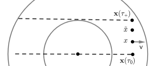
Figure 4. $\mathbf{x}(\tau_{+})$ and $\mathbf{x}(\tau_{0})$ for given $v$.

Lemma 3.8.

Assume that domain is given as in Definition 1.1. Fix $x,\bar{x}\in\Omega$, where $|x-\bar{x}|\leq 1$ and $v,\zeta\in\mathbb{R}^{3}$. We recall $\mathbf{x}(\tau)$ in (1.34). Assume $\tau_{*}\in[\text{min}\{\tau_{0},\tau_{+}\},\text{max}\{\tau_{0},\tau_{+}\}]$ and $(\mathbf{x}(\tau),v)\in\text{$\mathcal{C}_{1}$}$ with moving clockwise for $\tau\in[0,1]$ or $(\mathbf{x}(\tau),v)\in\text{$\mathcal{C}_{2}$}$ with moving clockwise for $\tau\in[0,1]$. Then we have

$$\Big{|}\int^{\tau_{+}}_{\tau_{*}}\frac{1}{\mathfrak{S}_{sp}(\tau;x,\tilde{x},v)}d\tau\Big{|}\lesssim\Big{(}\frac{1}{|v|_{p}}+\frac{1}{|v|_{p}\cos b(\mathbf{x}(\tau_{*}),v)}\Big{)}|\tau_{+}-\tau_{*}|,$$ (3.54)

where $\mathfrak{S}_{sp}(\tau;x,\tilde{x},v)$ is in Definition 1.12, and $b(x,v)$ is in (1.28) or (1.29).

Proof.

Assume $\tau_{*}\in[\text{min}\{\tau_{0},\tau_{+}\},\text{max}\{\tau_{0},\tau_{+}\}]$ and $(\mathbf{x}(\tau),v)\in\text{$\mathcal{C}_{1}$}$ with moving clockwise for $\tau\in[0,1]$. From (2.10),

$$0\leq\sin a(x,v)=\frac{r}{R}\sin b(x,v)\leq\frac{r}{R}$$ (3.55)

where $a(x,v),b(x,v)\in[0,\pi/2]$ are in (1.28). We have

$$\Big{|}\frac{X_{0}(\mathbf{x}(\tau),v)_{p}\cdot\frac{\dot{\mathbf{x}}(\tau)}{|\dot{\mathbf{x}}(\tau)|}}{X_{0}(\mathbf{x}(\tau),v)_{p}\cdot v}\Big{|}=\frac{\sin a(\mathbf{x}(\tau),v)}{|v|_{p}\cos a(\mathbf{x}(\tau),v)}\leq\frac{r}{|v|_{p}\sqrt{R^{2}-r^{2}}}\lesssim\frac{1}{|v|_{p}}.$$ (3.56)

Let $v=(v_{1},0,v_{3})$ and $v_{1}>0$ without loss of generality and $\mathbf{x}(\tau)_{p}=(|\mathbf{x}(\tau)|_{p}\cos\Theta(\tau),|\mathbf{x}(\tau)|_{p}\sin\Theta(\tau),0)=(\mathbf{x}(\tau)_{1},\mathbf{x}(\tau)_{2},0)$. From (2.9), we have

$$\sin b(\mathbf{x}(\tau),v)=\frac{|\mathbf{x}(\tau)|_{p}}{r}\sin(\Theta(\tau)-0)=\frac{\mathbf{x}(\tau)_{2}}{r}.$$

Then,

$$|X_{1}(\mathbf{x}(\tau),v)_{p}\cdot v|=r|v|_{p}\cos b(\mathbf{x}(\tau),v)=|v|_{p}\sqrt{r^{2}-\mathbf{x}(\tau)^{2}_{2}}$$

and since $v_{p}\;\bot\;\dot{\mathbf{x}}(\tau)$,

$$\Big{|}X_{1}(\mathbf{x}(\tau),v)_{p}\cdot\frac{\dot{\mathbf{x}}(\tau)}{|\dot{\mathbf{x}}(\tau)|}\Big{|}=r\sin b(\mathbf{x}(\tau),v)=\mathbf{x}(\tau)_{2}.$$

Recall $\mathbf{x}(\tau)_{2}=(1-\tau)\tilde{x}_{2}+\tau x_{2}$ for $\tilde{x}=(\tilde{x}_{1},\tilde{x}_{2},\tilde{x}_{3}),x=(x_{1},x_{2},x_{3})$ as in (1.34). If we perform change of variables, then we obtain

$$\Big{|}\int^{\tau_{+}}_{\tau_{*}}\frac{X_{1}(\mathbf{x}(\tau),v)_{p}\cdot\frac{\dot{\mathbf{x}}(\tau)}{|\dot{\mathbf{x}}(\tau)|}}{X_{1}(\mathbf{x}(\tau),v)_{p}\cdot v}d\tau\Big{|} =\Big{|}\int^{\tau_{+}}_{\tau_{*}}\frac{\mathbf{x}(\tau)_{2}}{|v|_{p}\sqrt{r^{2}-\mathbf{x}(\tau)^{2}_{2}}}d\tau\Big{|}$$

$$=\frac{1}{|v|_{p}|x_{2}-\tilde{x}_{2}|}\Big{|}\int^{\mathbf{x}(\tau_{+})}_{\mathbf{x}(\tau_{*})}\frac{t}{\sqrt{r^{2}-t^{2}}}dt\Big{|}$$

$$=\frac{1}{|v|_{p}|x_{2}-\tilde{x}_{2}|}|0-\sqrt{r^{2}-\mathbf{x}(\tau_{*})^{2}_{2}}|$$

$$=\frac{r}{|v|_{p}|x_{2}-\tilde{x}_{2}|}\cos b(\mathbf{x}(\tau_{*}),v)$$

since $\cos b(\mathbf{x}(\tau_{+}),v)=\sqrt{r^{2}-\mathbf{x}(\tau_{+})^{2}_{2}}/r=0$. From $\mathbf{x}(\tau_{*})_{2}-\mathbf{x}(\tau_{+})_{2}=(\tau_{+}-\tau_{*})(\tilde{x}_{2}-x_{2})$, we have

$$\frac{1}{\tilde{x}_{2}-x_{2}}=\frac{\tau_{+}-\tau_{*}}{\mathbf{x}(\tau_{*})_{2}-\mathbf{x}(\tau_{+})_{2}}=\frac{\tau_{+}-\tau_{*}}{r(\sin b(\mathbf{x}(\tau_{*}),v)-\sin b(\mathbf{x}(\tau_{+}),v))}=\frac{\tau_{+}-\tau_{*}}{r(\sin b(\mathbf{x}(\tau_{*}),v)-1)}.$$

Therefore, we obtain

$$\begin{split}\Big{|}\int^{\tau_{+}}_{\tau_{*}}\frac{X_{1}(\mathbf{x}(\tau),v)_{p}\cdot\frac{\dot{\mathbf{x}}(\tau)}{|\dot{\mathbf{x}}(\tau)|}}{X_{1}(\mathbf{x}(\tau),v)_{p}\cdot v}d\tau\Big{|}&\lesssim\frac{1}{|v_{p}|}\frac{\cos b(\mathbf{x}(\tau_{*}),v)}{1-\sin b(\mathbf{x}(\tau_{*}),v)}|\tau_{+}-\tau_{*}|\\ &=\frac{1+\sin b(\mathbf{x}(\tau_{*}),v)}{|v|_{p}\cos b(\mathbf{x}(\tau_{*}),v)}|\tau_{+}-\tau_{*}|\\ &\lesssim\frac{1}{|v|_{p}\cos b(\mathbf{x}(\tau_{*}),v)}|\tau_{+}-\tau_{*}|.\end{split}$$ (3.57)

From (3.56) and (3.57), we conclude

$$\Big{|}\int^{\tau_{+}}_{\tau_{*}}\frac{1}{\mathfrak{S}_{sp}(\tau;x,\tilde{x},v)}d\tau\Big{|} =\Big{|}\int^{\tau_{+}}_{\tau_{*}}\frac{1}{\mathfrak{S}_{sp}^{1}(\tau;x,\tilde{x},v)}d\tau+\int^{\tau_{+}}_{\tau_{*}}\frac{1}{\mathfrak{S}_{sp}^{2}(\tau;x,\tilde{x},v)}d\tau\Big{|}$$

$$\leq\Big{|}\int^{\tau_{+}}_{\tau_{*}}\frac{X_{0}(\mathbf{x}(\tau),v)_{p}\cdot\frac{\dot{\mathbf{x}}(\tau)}{|\dot{\mathbf{x}}(\tau)|}}{X_{0}(\mathbf{x}(\tau),v)_{p}\cdot v}d\tau\Big{|}+\Big{|}\int^{\tau_{+}}_{\tau_{*}}\frac{X_{1}(\mathbf{x}(\tau),v)_{p}\cdot\frac{\dot{\mathbf{x}}(\tau)}{|\dot{\mathbf{x}}(\tau)|}}{X_{1}(\mathbf{x}(\tau),v)_{p}\cdot v}d\tau\Big{|}$$

$$\lesssim\Big{(}\frac{1}{|v|_{p}}+\frac{1}{|v|_{p}\cos b(\mathbf{x}(\tau_{*}),v)}\Big{)}|\tau_{+}-\tau_{*}|,$$

where $b(x,v)$ is in (1.28). If $(\mathbf{x}(\tau),v)\in\mathcal{C}_{2}$ with moving clockwise for $\tau\in[0,1]$, we can use same arguments as in $\mathcal{C}_{1}$. ∎

Definition 3.9.

Suppose the domain is given as in Definition 1.1. Fix $x\in\Omega,v,\bar{v},\zeta\in\mathbb{R}^{3}$. We recall $\mathbf{v}(\tau)$ in (1.37). When $X(s;t,x,\mathbf{v}(\tau))$ with moving clockwise for all $\tau\in[0,1]$, we define $\tau_{+}(x,v,\bar{v},\zeta)$ and $\tau_{0+}(x,v,\bar{v},\zeta)$ as

$$\begin{split}&\widehat{\mathbf{v}(\tau_{+})}\cdot n(X_{1}(x,\mathbf{v}(\tau_{+})))=0,\quad\tau_{+}=\tau_{+}(x,v,\bar{v},\zeta),\\ &\widehat{\mathbf{v}(\tau_{0+})}\cdot n(X_{1}(x,\mathbf{v}(\tau_{0+})))=-1,\quad\tau_{0+}=\tau_{0+}(x,v,\bar{v},\zeta),\end{split}$$ (3.58)

where $(x,\mathbf{v}(\tau_{+})),(x,\mathbf{v}(\tau_{0+}))\in\text{$\mathcal{C}_{1}$}$.(See the left side of the Figure 5).

We define $\tau_{-}(x,v,\bar{v},\zeta)$ and $\tau_{0-}(x,v,\bar{v},\zeta)$ as

$$\begin{split}&\widehat{\mathbf{v}(\tau_{-})}\cdot n(X_{0}(x,\mathbf{v}(\tau_{-})))=0,\quad\tau_{-}=\tau_{-}(x,v,\bar{v},\zeta),\\ &\widehat{\mathbf{v}(\tau_{0-})}\cdot n(X_{0}(x,\mathbf{v}(\tau_{0-})))=1,\quad\tau_{0-}=\tau_{0-}(x,v,\bar{v},\zeta),\end{split}$$ (3.59)

where $(x,\mathbf{v}(\tau_{-})),(x,\mathbf{v}(\tau_{0-}))\in\text{$\mathcal{C}_{2}$}$.(See the right side of the Figure 5).

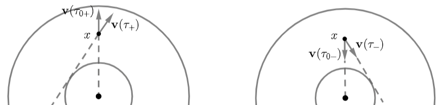
Figure 5. $\mathbf{v}(\tau_{+}),\mathbf{v}(\tau_{0+}),\mathbf{v}(\tau_{-})$ and $\mathbf{v}(\tau_{0-})$ for given $x$.

Lemma 3.10.

Suppose the domain is given as in Definition 1.1. Fix any $x\in\Omega,v,\bar{v},\zeta\in\mathbb{R}^{3}$. We recall $\mathbf{v}(\tau)$ in (1.37).
(i) Assume $\tau_{*}\in[\text{min}\{\tau_{0+},\tau_{+}\},\text{max}\{\tau_{0+},\tau_{+}\}]$ and $(x,\mathbf{v}(\tau))\in\text{$\mathcal{C}_{1}$}$ with moving clockwise. Then we have

$$\Big{|}\int^{\tau_{+}}_{\tau_{*}}\frac{1}{\mathfrak{S}_{vel}(\tau;x,v,\tilde{v},\zeta)}d\tau\Big{|}\lesssim\Big{(}\frac{1}{|v+\zeta|^{2}_{p}}+\frac{1}{\cos b(x,\mathbf{v}(\tau_{*}))}\frac{1}{|v+\zeta|^{2}_{p}}\Big{)}|\tau_{+}-\tau_{*}|,$$ (3.60)

where $\mathfrak{S}_{vel}(\tau;x,v,\tilde{v},\zeta)$ is in Definition 1.12, and $b(x,v)$ is in (1.28).

(ii) Assume $\tau_{*}\in[\text{min}\{\tau_{0-},\tau_{-}\},\text{max}\{\tau_{0-},\tau_{-}\}]$ and $(x,\mathbf{v}(\tau))\in\text{$\mathcal{C}_{2}$}$ with moving clockwise. Then we have

$$\Big{|}\int^{\tau_{-}}_{\tau_{*}}\frac{1}{\mathfrak{S}_{vel}(\tau;x,v,\tilde{v},\zeta)}d\tau\Big{|}\lesssim\Big{(}\frac{1}{|v+\zeta|^{2}_{p}}+\frac{1}{\cos b(x,\mathbf{v}(\tau_{*}))}\frac{1}{|v+\zeta|^{2}_{p}}\Big{)}|\tau_{-}-\tau_{*}|,$$ (3.61)

where $b(x,v)$ is in (1.29).

Proof.

(i) Using (3.55),

$$\begin{split}t_{f}(x,\mathbf{v}(\tau))\Big{|}\frac{X_{0}(x,\mathbf{v}(\tau))_{p}\cdot\frac{\dot{\mathbf{v}}(\tau)}{|\dot{\mathbf{v}}(\tau)|}}{X_{0}(x,\mathbf{v}(\tau))_{p}\cdot\mathbf{v}(\tau)}\Big{|}&\leq t_{*}(x,\mathbf{v}(\tau))\frac{1}{|\mathbf{v}(\tau)|_{p}\cos a(x,\mathbf{v}(\tau))}\\ &\lesssim\frac{1}{|v+\zeta|^{2}_{p}}\frac{1}{\sqrt{1-(r/R)^{2}}}\lesssim\frac{1}{|v+\zeta|^{2}_{p}}\end{split}$$ (3.62)

since $t_{f}(x,\mathbf{v}(\tau))\leq t_{*}(x,\mathbf{v}(\tau))\lesssim 1/|v+\zeta|_{p}$. Now, we let $x=(0,x_{2},x_{3})$ and $x_{2}>0$ without loss of generality and

$$(\tilde{v}+\zeta)_{p}=(|v+\zeta|_{p}\cos\theta(\tilde{v}),|v+\zeta|_{p}\sin\theta(\tilde{v}),0),$$

$$(v+\zeta)_{p}=(|v+\zeta|_{p}\cos\theta(v),|v+\zeta|_{p}\sin\theta(v),0).$$

Let us $\Theta(0)=\theta(\tilde{v})$ and $\Theta(1)=\theta(v)$. We redefine $\mathbf{v}(\tau)_{p}=(|v+\zeta|_{p}\cos\Theta(\tau),|v+\zeta|_{p}\sin\Theta(\tau),0)$ for $\Theta(\tau)=(\Theta(1)-\Theta(0))\tau+\Theta(0)$ for convenience. From (2.9), we have

$$\sin b(x,\mathbf{v}(\tau))=\frac{|x|_{p}}{r}\sin(\frac{\pi}{2}-\Theta(\tau))=\frac{|x|_{p}}{r}\cos\Theta(\tau).$$

Then,

$$|X_{1}(x,\mathbf{v}(\tau))_{p}\cdot\mathbf{v}(\tau)|=r|v+\zeta|_{p}\cos b(x,\mathbf{v}(\tau))=|v+\zeta|_{p}\sqrt{r^{2}-|x|^{2}_{p}\cos^{2}\Theta(\tau)}$$

and since $\mathbf{v}(\tau)_{p}\;\bot\;\dot{\mathbf{v}}(\tau)$,

$$\Big{|}X_{1}(x,\mathbf{v}(\tau))_{p}\cdot\frac{\dot{\mathbf{v}}(\tau)}{|\dot{\mathbf{v}}(\tau)|}\Big{|}=r\sin b(x,\mathbf{v}(\tau))=|x|_{p}\cos\Theta(\tau).$$

From (3.58) and Figure 5, we have

$$\sin\Theta(\tau_{+})=\frac{\sqrt{|x|^{2}_{p}-r^{2}}}{|x|_{p}},\quad\sin\Theta(\tau_{0+})=1.$$

It holds that

$$\frac{\sqrt{|x|^{2}_{p}-r^{2}}}{|x|_{p}}\leq\sin\Theta(\tau)\leq 1$$ (3.63)

since $\tau$ is in between $\tau_{+}$ and $\tau_{0+}$. Also, we have

$$t_{b}(x,\mathbf{v}(\tau))\leq t_{b}(x,\mathbf{v}(\tau_{+}))\leq\frac{\sqrt{|x|^{2}_{p}-r^{2}}}{|v+\zeta|_{p}}$$ (3.64)

since $\tau$ is in between $\tau_{+}$ and $\tau_{0+}$. The Jacobian determinant is obtained by

$$\Big{|}\frac{d\tau}{dt}\Big{|}=\frac{1}{|x|_{p}\sin\Theta(\tau)}\frac{1}{|\Theta(1)-\Theta(0)|}\in(0,\infty),$$

where $t=|x|_{p}\cos\Theta(\tau)$. If we perform change of variables, then we obtain

$$\begin{split}&\Big{|}\int^{\tau_{+}}_{\tau_{*}}t_{b}(x,\mathbf{v}(\tau))\frac{X_{1}(x,\mathbf{v}(\tau))_{p}\cdot\frac{\dot{\mathbf{v}}(\tau)}{|\dot{\mathbf{v}}(\tau)|}}{X_{1}(x,\mathbf{v}(\tau))_{p}\cdot\mathbf{v}(\tau)}d\tau\Big{|}\\ &=\frac{1}{|v+\zeta|_{p}|\Theta(1)-\Theta(0)|}\Big{|}\int^{|x|_{p}\cos\Theta(\tau_{+})}_{|x|_{p}\cos\Theta(\tau_{*})}t_{b}(x,\mathbf{v}(\tau))\frac{1}{\sin\Theta(\tau)}\frac{t}{\sqrt{r^{2}-t^{2}}}dt\Big{|}.\end{split}$$ (3.65)

By (3.63) and (3.64), we obtain

$$\eqref{est:g:temp} \leq\frac{|x|_{p}}{|v+\zeta|^{2}_{p}|\Theta(1)-\Theta(0)|}\int^{|x|_{p}\cos\Theta(\tau_{+})}_{|x|_{p}\cos\Theta(\tau_{*})}\frac{t}{\sqrt{r^{2}-t^{2}}}dt\Big{|}$$

$$\leq\frac{|x|_{p}}{|v+\zeta|^{2}_{p}|\Theta(1)-\Theta(0)|}|0-\sqrt{r^{2}-|x|^{2}_{o}\cos^{2}\Theta(\tau_{*})}|$$

$$=\frac{|x|_{p}}{|v+\zeta|^{2}_{p}|\Theta(1)-\Theta(0)|}\cos b(x,\mathbf{v}(\tau_{*}))$$

since $\cos\Theta(\tau_{+})=r/|x|_{p}$. It holds that

$$\Theta(\tau_{*})-\Theta(\tau_{+})=(\Theta(1)-\Theta(0))(\tau_{*}-\tau_{+})$$

and

$$|\Theta(\tau_{*})-\Theta(\tau_{+})| \geq|\cos\Theta(\tau_{*})-\cos\Theta(\tau_{+})|=\Big{|}\frac{r}{|x|_{p}}\sin b(x,\mathbf{v}(\tau_{*}))-\frac{r}{|x|_{p}}\Big{|}$$

$$\geq\frac{r}{|x|_{p}}|\sin b(x,\mathbf{v}(\tau_{*}))-1|.$$

Therefore, we obtain

$$\begin{split}&\Big{|}\int^{\tau_{+}}_{\tau_{*}}t_{b}(x,\mathbf{v}(\tau))\frac{X_{1}(x,\mathbf{v}(\tau))_{p}\cdot\frac{\dot{\mathbf{v}}(\tau)}{|\dot{\mathbf{v}}(\tau)|}}{X_{1}(x,\mathbf{v}(\tau))_{p}\cdot\mathbf{v}(\tau)}d\tau\Big{|}\\ &\lesssim\frac{1}{|v+\zeta|_{p}^{2}}\frac{\cos b(x,\mathbf{v}(\tau_{*}))}{1-\sin b(x,\mathbf{v}(\tau_{*})}|\tau_{+}-\tau_{*}|\lesssim\frac{1}{|v+\zeta|_{p}^{2}}\frac{1}{\cos b(x,\mathbf{v}(\tau_{*})}|\tau_{+}-\tau_{*}|.\end{split}$$ (3.66)

Using (3.62) and (3.66), we conclude

$$\quad\Big{|}\int^{\tau_{+}}_{\tau_{*}}\frac{1}{\mathfrak{S}_{vel}(\tau;x,v,\tilde{v},\zeta)}d\tau\Big{|}$$

$$=\Big{|}\int^{\tau_{+}}_{\tau_{*}}\frac{1}{\mathfrak{S}_{vel}^{1}(\tau;x,v,\tilde{v},\zeta)}d\tau+\int^{\tau_{+}}_{\tau_{*}}\frac{1}{\mathfrak{S}_{vel}^{2}(\tau;x,v,\tilde{v},\zeta)}d\tau\Big{|}$$

$$\leq\Big{|}\int^{\tau_{+}}_{\tau_{*}}t_{f}(x,\mathbf{v}(\tau))\frac{X_{0}(x,\mathbf{v}(\tau))_{p}\cdot\frac{\dot{\mathbf{v}}(\tau)}{|\dot{\mathbf{v}}(\tau)|}}{X_{0}(x,\mathbf{v}(\tau))_{p}\cdot\mathbf{v}(\tau)}d\tau\Big{|}+\Big{|}\int^{\tau_{+}}_{\tau_{*}}t_{b}(x,\mathbf{v}(\tau))\frac{X_{1}(x,\mathbf{v}(\tau))_{p}\cdot\frac{\dot{\mathbf{v}}(\tau)}{|\dot{\mathbf{v}}(\tau)|}}{X_{1}(x,\mathbf{v}(\tau))_{p}\cdot\mathbf{v}(\tau)}d\tau\Big{|}$$

$$\lesssim\Big{(}\frac{1}{|v+\zeta|^{2}_{p}}+\frac{1}{\cos b(x,\mathbf{v}(\tau_{*}))}\frac{1}{|v+\zeta|^{2}_{p}}\Big{)}|\tau_{+}-\tau_{*}|,$$

where $b(x,v)$ is in (1.28). If $(x,\mathbf{v}(\tau))\in\mathcal{C}_{2}$ with moving clockwise, we can use same arguments as in $\mathcal{C}_{1}$. ∎

4. Difference quotients estimates for $\mathcal{C}_{3}$

In section 4, we let $f:\overline{\Omega}\times\mathbb{R}^{3}\rightarrow\mathbb{R}_{+}\cup\{0\}$ be a function which satisfies specular reflection (1.4), where $\Omega$ is a domain as in Definition 1.1 and $w(v)=e^{\vartheta|v|^{2}}$ for some $0<\vartheta$. For $x,\bar{x}\in\Omega$, $v,\bar{v},\zeta\in\mathbb{R}^{3}$, we assume (1.32), and recall $\tilde{x}(x,\bar{x},v+\zeta)$ in (1.33). We also assume (1.35), and recall $\tilde{v}(v,\bar{v},\zeta)$ in (1.36).

4.1. Nonsingular part of $\mathcal{C}_{3}$

Lemma 4.1.

Fix any point $t,s\in\mathbb{R}^{+}$, $v,\zeta\in\mathbb{R}^{3}$, $x,\bar{x}\in\Omega$. Assume that $(\tilde{x},v+\zeta),(\bar{x},v+\zeta)\in\mathcal{C}_{3}$ with moving clockwise. For $|x-\bar{x}|\leq 1$,

$$\begin{split}&|f(s,X(s;t,\tilde{x},v+\zeta),V(s;t,\tilde{x},v+\zeta))-f(s,X(s;t,\bar{x},v+\zeta),V(s;t,\bar{x},v+\zeta))|/|x-\bar{x}|^{\gamma}\\ \lesssim\;&\Big{[}\frac{e^{\varpi\langle v+\zeta\rangle^{2}s}}{\langle v+\zeta\rangle}\sup_{\begin{subarray}{c}v\in\mathbb{R}^{3}\\ 0<|x-\bar{x}|\leq 1\end{subarray}}\Big{(}e^{-\varpi\langle v\rangle^{2}s}\langle v\rangle\frac{|f(s,x,v)-f(s,\bar{x},v)|}{|x-\bar{x}|^{\gamma}}\Big{)}+\frac{\|wf(s)\|_{\infty}}{w(v+\zeta)}\Big{]}\\ &+|v+\zeta|_{p}^{\gamma}\times\Big{[}\frac{e^{\varpi\langle v+\zeta\rangle^{2}s}}{\langle v+\zeta\rangle^{2}}\sup_{\begin{subarray}{c}x\in\Omega\\ 0<|v-\bar{v}|\leq 1\end{subarray}}\Big{(}e^{-\varpi\langle v\rangle^{2}s}\langle v\rangle^{2}\frac{|f(s,x,v)-f(s,x,\bar{v})|}{|v-\bar{v}|^{\gamma}}\Big{)}+\frac{\|wf(s)\|_{\infty}}{w(v+\zeta)}\Big{]}.\end{split}$$ (4.1)

Proof.

The proof is the same as in Lemma 3.1. ∎

Lemma 4.2.

Fix any point $t,s\in\mathbb{R}^{+}$, $x,\bar{x}\in\Omega$, and $v,\bar{v},\zeta\in\mathbb{R}^{3}$. Assume that $(x,\tilde{v}+\zeta),(x,\bar{v}+\zeta)\in\mathcal{C}_{3}$ with moving clockwise. For $\tilde{v}(v,\bar{v},\zeta)$,

$$\begin{split}&\quad|f(s,X(s;t,x,\tilde{v}+\zeta),V(s;t,x,\tilde{v}+\zeta))-f(s,X(s;t,x,\bar{v}+\zeta),V(s;t,x,\bar{v}+\zeta))|/|v-\bar{v}|^{\gamma}\\ &\lesssim\;\Big{[}(t-s)+\text{max}\{|v+\zeta|_{p}^{-1},|\bar{v}+\zeta|_{p}^{-1}\}\Big{]}^{\gamma}\\ &\quad\quad\times\Big{[}\frac{e^{\varpi\langle v+\zeta\rangle^{2}s}}{\langle v+\zeta\rangle}\sup_{\begin{subarray}{c}v\in\mathbb{R}^{3}\\ 0<|x-\bar{x}|\leq 1\end{subarray}}\Big{(}e^{-\varpi\langle v\rangle^{2}s}\langle v\rangle\frac{|f(s,x,v)-f(s,\bar{x},v)|}{|x-\bar{x}|^{\gamma}}\Big{)}+\frac{\|wf(s)\|_{\infty}}{w(v+\zeta)}\Big{]}\\ &\quad+\Big{[}1+(t-s)\text{max}\{|v+\zeta|_{p},|\bar{v}+\zeta|_{p}\}\Big{]}^{\gamma}\\ &\quad\quad\times\Big{[}\frac{e^{\varpi\langle v+\zeta\rangle^{2}s}}{\langle v+\zeta\rangle^{2}}\sup_{\begin{subarray}{c}x\in\Omega\\ 0<|v-\bar{v}|\leq 1\end{subarray}}\Big{(}e^{-\varpi\langle v\rangle^{2}s}\langle v\rangle^{2}\frac{|f(s,x,v)-f(s,x,\bar{v})|}{|v-\bar{v}|^{\gamma}}\Big{)}+\frac{\|wf(s)\|_{\infty}}{w(v+\zeta)}\Big{]}.\end{split}$$ (4.2)

Proof.

We denote $\tilde{v}:=\tilde{v}+\zeta$, $\bar{v}:=\bar{v}+\zeta$, $m(s;t,x,\bar{v}):=m$ and $m(s;t,x,\tilde{v}):=n$. Without loss of generality, we let $m\geq n$. Since $\tilde{v}_{p}$ and $\bar{v}_{p}$ have the same direction,

$$a(x,\tilde{v})=a(x,\bar{v}),\quad l(x,\tilde{v})=l(x,\bar{v})=2R\cos a(x,\tilde{v}),$$

where $a(x,v)$ is in (1.30), and $l(x,v)$ is in (1.23). We have

$$\begin{split}&|t_{b}(x,\tilde{v})-t_{b}(x,\bar{v})|=|X_{1}(x,\tilde{v})-x|_{p}\Big{|}\frac{1}{|\tilde{v}|_{p}}-\frac{1}{|\bar{v}|_{p}}\Big{|}\lesssim\frac{|v-\bar{v}|}{|\bar{v}|_{p}|\tilde{v}|_{p}},\\ &|t_{*}(x,\tilde{v})-t_{*}(x,\bar{v})|=|2R\cos a(x,\tilde{v})|\Big{|}\frac{1}{|\tilde{v}|_{p}}-\frac{1}{|\bar{v}|_{p}}\Big{|}\lesssim\cos a(x,\tilde{v})\frac{|v-\bar{v}|}{|\bar{v}|_{p}|\tilde{v}|_{p}}.\end{split}$$ (4.3)

By definition of $m(s;t,x,v)$ in (2.7), $m,n\in\mathbb{N}\cup\{0\}$ satisfy

$$\begin{split}&m-1\leq\frac{t-s-t_{b}(x,\bar{v})}{t_{*}(x,\bar{v})}=(t-s-t_{b}(x,\bar{v}))\frac{|\bar{v}|_{p}}{l(x,\bar{v})}\leq\frac{|\bar{v}|_{p}(t-s-t_{b}(x,\bar{v}))}{2R\cos a(x,\tilde{v})},\\ &n>\frac{t-s-t_{b}(x,\tilde{v})}{t_{*}(x,\tilde{v})}=(t-s-t_{b}(x,\tilde{v}))\frac{|\tilde{v}|_{p}}{l(x,\tilde{v})}\geq\frac{|\tilde{v}|_{p}(t-s-t_{b}(x,\tilde{v}))}{2R\cos a(x,\tilde{v})}\end{split}$$ (4.4)

since $\cos a(x,\bar{v}),\cos a(x,\tilde{v})>0$, and $s\in[0,t]$ satisfies

$$t_{n+1}(t,x,\tilde{v})<s\leq t_{n}(t,x,\tilde{v})\quad\text{and}\quad t_{m+1}(t,x,\bar{v})<s\leq t_{m}(t,x,\bar{v}),$$ (4.5)

where $t_{n}(t,x,v)$ is in (2.8). From (2.14) and (2.18),

$$\theta_{X_{m}}(x,\bar{v})-\theta_{X_{n}}(x,\tilde{v})=\theta_{V_{m}}(x,\bar{v})-\theta_{V_{n}}(x,\tilde{v})=(m-n)(\pi-2a(x,\tilde{v})).$$

We have

$$\quad|V(s;t,x,\bar{v})-V(s;t,x,\tilde{v})|\leq|\tilde{v}|_{p}|\sin\Big{(}(m-n)(\pi/2-a(x,\tilde{v}))\Big{)}|+|\tilde{v}-\bar{v}|$$ (4.6)

and

$$\quad|X(s;t,x,\bar{v})-X(s;t,x,\tilde{v})|$$

$$\leq|X_{m}(x,\bar{v})-X_{n}(x,\tilde{v})|_{p}+|V_{m}(x,\bar{v})-V_{n}(x,\tilde{v})|_{p}|t_{n}(t,x,\tilde{v})-s|+|\bar{v}|_{p}|t_{n}(t,x,\tilde{v})-t_{m}(t,x,\bar{v})|$$

$$\quad+|\tilde{v}_{3}-\bar{v}_{3}|(t-s)$$

$$\lesssim|\sin\Big{(}(m-n)(\pi/2-a(x,\tilde{v}))\Big{)}|+|\bar{v}|_{p}|t_{b}(x,\tilde{v})-t_{b}(x,\bar{v})|$$

$$\quad+|\bar{v}|_{p}|(n-1)(t_{*}(x,\tilde{v})-t_{*}(x,\bar{v}))|+(m-n)|\bar{v}|_{p}t_{*}(x,\bar{v})+|v-\bar{v}|\Big{(}(t-s)+\frac{1}{|\tilde{v}|_{p}}\Big{)}$$ (4.7)

since $|t_{n}(t,x,\tilde{v})-s|\leq t_{*}(x,\tilde{v})\lesssim\frac{1}{|\tilde{v}|_{p}}$.

We first assume that $m\geq n+2$. Applying (4.3) and (4.4),

$$(m-n)(\pi/2-a(x,\tilde{v}))\leq 2(m-n-1)(\pi/2-a(x,\tilde{v}))\leq|v-\bar{v}|\Big{(}(t-s)+\frac{1}{|\bar{v}|_{p}}\Big{)}$$ (4.8)

since $\cos a(x,\tilde{v})\geq\frac{2}{\pi}\Big{(}\frac{\pi}{2}-a(x,\tilde{v})\Big{)}$. Similarly,

$$(m-n)t_{*}(x,\bar{v})|\bar{v}|_{p}\leq|v-\bar{v}|\Big{(}(t-s)+\frac{1}{|\bar{v}|_{p}}\Big{)}$$ (4.9)

by using $t_{*}(x,\bar{v})=2R\cos a(x,\tilde{v})/|\bar{v}|_{p}$. Applying (4.8) to (4.6),

$$\quad|V(s;t,x,\bar{v})-V(s;t,x,\tilde{v})|\leq|v-\bar{v}|\Big{(}\text{max}\{|\bar{v}|_{p},|\tilde{v}|_{p}\}(t-s)+1\Big{)}.$$

Applying (4.8) and (4.9) to (4.1),

$$|X(s;t,x,\bar{v})-X(s;t,x,\tilde{v})|\lesssim|v-\tilde{v}|\Big{(}(t-s)+\text{max}\{\frac{1}{|v|_{p}},\frac{1}{|\bar{v}|_{p}}\}\Big{)}.$$

Next, we assume $m=n$. From (4.6) and (4.1),

$$\begin{split}&\quad|V(s;t,x,\bar{v})-V(s;t,x,\tilde{v})|\leq|v-\bar{v}|\\ &\quad|X(s;t,x,\bar{v})-X(s;t,x,\tilde{v})|\leq|v-\bar{v}|\Big{(}(t-s)+\text{max}\{\frac{1}{|v|_{p}},\frac{1}{|\bar{v}|_{p}}\}\Big{)}.\end{split}$$ (4.10)

We assume that $m=n+1$. Recall (3.16),

$$|f(s,X(s;t,x,\tilde{v}),V(s;t,x,\tilde{v}))-f(s,X(s;t,x,\bar{v}),V(s;t,x,\bar{v}))|$$

$$\leq|f(s,X(s;t,x,\tilde{v}),V(s;t,x,\tilde{v}))-f(s,X_{n+1}^{*}(x,\tilde{v}),V(s;t,x,\tilde{v}))|$$

$$\quad+|f(s,X_{n+1}^{*}(x,\tilde{v}),V_{n+1}(x,\tilde{v}))-f(s,X(s;t,x,\bar{v}),V(s;t,x,\bar{v}))|,$$

where $X_{n+1}^{*}(x,\tilde{v})$ is in (3.15). Similar to (3.17) and (3.18),

$$|X(s;t,x,\tilde{v})-X_{n+1}^{*}(x,\tilde{v})|\leq|v-\bar{v}|\Big{(}(t-s)+\text{max}\{\frac{1}{|v|_{p}},\frac{1}{|\bar{v}|_{p}}\}\Big{)}$$ (4.11)

and

$$\begin{split}|X_{n+1}^{*}(x,\tilde{v})-X(s;t,x,\bar{v})|\lesssim|v-\bar{v}|\Big{(}(t-s)+\text{max}\{\frac{1}{|v|_{p}},\frac{1}{|\bar{v}|_{p}}\}\Big{)}.\end{split}$$ (4.12)

Therefore, we can construct (4.2) by (4.10), (4.11), and (4.12). ∎

4.2. Singular part of $\mathcal{C}_{3}$

Ko and Lee obtained $\nabla_{x}X(0;t;x,v),\nabla_{x}V(0;t,x,v)$, $\nabla_{v}X(0;t,x,v)$, and $\nabla_{v}V(0;t,x,v)$ in a disk with the specular reflection boundary condition in [33]. Before starting this section, we recall Lemma 5.4 of [33].

Lemma 4.3.

Let $(t,x,v)\in\mathbb{R}^{+}\times O\times\mathbb{R}^{2}$, where $O=\{x\in\mathbb{R}^{2}:|x|=1\}$. We assume that $n(x_{\mathbf{b}})\cdot v\neq 0$, where $n(x_{\mathbf{b}})$ is outward unit normal vector at $x_{\mathbf{b}}=x-t_{\mathbf{b}}v\in\partial O$. Then we have estimates of derivatives for the characteristics $X(0;t,x,v)$ and $V(0;t,x,v)$

$$|\nabla_{x}X(0,t,x,v)|\lesssim\frac{|v|}{|v\cdot n(x_{\mathbf{b}})|}(1+|v|t),$$

$$|\nabla_{v}X(0,t,x,v)|\lesssim\frac{1}{|v|}(1+|v|t),$$

$$|\nabla_{x}V(0,t,x,v)|\lesssim\frac{|v|^{3}}{|v\cdot n(x_{\mathbf{b}})|^{2}}(1+|v|t),$$

$$|\nabla_{v}V(0,t,x,v)|\lesssim\frac{|v|}{|v\cdot n(x_{\mathbf{b}})|}(1+|v|t).$$

Proof.

We refer Lemma 5.4 of [33]. ∎

Figure 6. When $v$ is fixed, the possible location of $x$.

Lemma 4.4.

Fix any point $t,s\in\mathbb{R}^{+}$, $v\in\mathbb{R}^{3}$, $x,\bar{x}\in\Omega$. Assume that $(\mathbf{x}(\tau),v)\in\mathcal{C}_{3}$ with moving clockwise for all $\tau\in[0,1]$. For $|x-\bar{x}|\leq 1$,

$$\begin{split}|X(s;t,x,v)-X(s;t,\tilde{x},v)|\lesssim\text{max}\{\frac{1}{\cos a(x,v)},\frac{1}{\cos a(\tilde{x},v)}\}(1+|v|_{p}(t-s))|x-\bar{x}|,\\ |V(s;t,x,v)-V(s;t,\tilde{x},v)|\lesssim\text{max}\{\frac{1}{\cos^{2}a(x,v)},\frac{1}{\cos^{2}a(\tilde{x},v)}\}(|v|_{p}+|v|_{p}^{2}(t-s))|x-\bar{x}|,\end{split}$$ (4.13)

where $a(x,v)$ is in (1.30).

Proof.

For $v=(|v|_{p}\cos\theta_{v},|v|_{p}\sin\theta_{v},v_{3})$, we assume $\theta_{v}=0$ without loss of generality. Then we have $v=(v_{1},0,v_{3})$. From Lemma 4.3,

$$|\nabla_{x_{1},x_{2}}X(s;t,x_{p},v_{p})|\lesssim\frac{|v|_{p}}{|v_{p}\cdot n({x}_{p,b})|}(1+|v|_{p}(t-s))$$

and

$$|\nabla_{x_{1},x_{2}}V(s;t,x_{p},v_{p})|\lesssim\frac{|v|_{p}^{3}}{|v_{p}\cdot n(x_{p,b})|^{2}}(1+|v|_{p}(t-s)),$$

where $n(x_{p,b})$ is outward unit normal vector at $x_{p,b}=x_{p}-t_{b}v_{p}\in\partial\Omega$. In this paper,

$$v_{p}\cdot n(x_{p,b})=v_{p}\cdot n(X_{1}(x_{p},v_{p}))=v_{p}\cdot X_{1}(x,v)_{p}=-|v|_{p}\cos a(x,v).$$

Since $X(s;t,x,v)_{ver}=(0,0,x_{3}-(t-s)v_{3})$ and $V(s;t,x,v)=v_{3}$ for $x=(x_{1},x_{2},x_{3}),v=(v_{1},v_{2},v_{3})$,

$$\nabla_{x_{3}}X(s;t,x,v)=1\text{\quad and \quad}\nabla_{x_{3}}V(s;t,x,v)=0.$$

From (2.9), we have $\sin a(\mathbf{x}(\tau),v)=\mathbf{x}(\tau)\cdot(0,1,0)$. Thus, by Figure 6,

$$\max_{\tau}\{\frac{1}{\cos a(\mathbf{x}(\tau),v)}\}=\text{max}\{\frac{1}{\cos a(x,v)},\frac{1}{\cos a(\tilde{x},v)}\}$$

and

$$\max_{\tau}\{\frac{1}{\cos^{2}a(\mathbf{x}(\tau),v)}\}=\text{max}\{\frac{1}{\cos^{2}a(x,v)},\frac{1}{\cos^{2}a(\tilde{x},v)}\}.$$

Therefore,

$$|X(s;t,x,v)-X(s;t,\tilde{x},v)|$$

$$\leq\int^{1}_{0}|\nabla_{x}X(s;t,\mathbf{x}(\tau),v)\dot{\mathbf{x}}|d\tau$$

$$\lesssim|x-\tilde{x}|\times\text{max}\{\frac{1}{\cos a(x,v)},\frac{1}{\cos a(\tilde{x},v)}\}(1+|v|_{p}(t-s))$$

and

$$|V(s;t,x,v)-V(s;t,\tilde{x},v)|$$

$$\leq\int^{1}_{0}|\nabla_{x}V(s;t,\mathbf{x}(\tau),v)\dot{\mathbf{x}}|d\tau$$

$$\lesssim|x-\tilde{x}|\times\text{max}\{\frac{1}{\cos^{2}a(x,v)},\frac{1}{\cos^{2}a(\tilde{x},v)}\}(|v|_{p}+|v|_{p}^{2}(t-s)).$$

∎

Lemma 4.5.

Assume that $\Omega$ is a domain as in Definition 1.1. Fix $x\in\Omega$ and $v,\bar{v},\zeta\in\mathbb{R}^{3}$. Assume that $(x,v+\zeta),(x,\tilde{v}+\zeta)\in\mathcal{C}_{3}$ with moving clockwise, and $x_{p}\cdot v$ and $x_{p}\cdot\tilde{v}$ have the same sign. For $\tilde{v}(v,\bar{v},\zeta)$,

$$\begin{split}&|t_{b}(x,v+\zeta)-t_{b}(x,\tilde{v}+\zeta)|\lesssim\frac{1}{|v+\zeta|^{2}_{p}}|v-\tilde{v}|,\\ &|t_{f}(x,v+\zeta)-t_{f}(x,\tilde{v}+\zeta)|\lesssim\frac{1}{|v+\zeta|^{2}_{p}}|v-\tilde{v}|,\\ &|t_{*}(x,v+\zeta)-t_{*}(x,\tilde{v}+\zeta)|\lesssim\frac{1}{|v+\zeta|^{2}_{p}}|v-\tilde{v}|,\\ \end{split}$$ (4.14)

and

$$\begin{split}&|\cos a(x,v+\zeta)-\cos a(x,\tilde{v}+\zeta)|\lesssim\frac{1}{|v+\zeta|_{p}}|v-\tilde{v}|,\\ &|a(x,v+\zeta)-a(x,\tilde{v}+\zeta)|\lesssim|v+\zeta|^{-1}_{p}\frac{1}{|v+\zeta|_{p}}|v-\tilde{v}|,\end{split}$$ (4.15)

where $a(x,v)$ is in (1.30).

Proof.

Since $|X_{0}(x,v)|_{p}=|(x_{1}+t_{f}(x,v)v_{1},x_{2}+t_{f}(x,v)v_{2},0)|=R$,

$$|v|_{p}^{2}t_{f}(x,v)=-(x_{p}\cdot v_{p})+\sqrt{(x_{p}\cdot v_{p})^{2}+|v|_{p}^{2}(R^{2}-|x|_{p}^{2})}.$$ (4.16)

It holds that

$$\begin{split}&\quad|v|_{p}^{2}|t_{f}(x,v)-t_{f}(x,\tilde{v})|\\ &\leq|(v_{p}-\tilde{v}_{p})\cdot x_{p}|+|\sqrt{(x_{p}\cdot v_{p})^{2}+|v|_{p}^{2}(R^{2}-|x|_{p}^{2})}-\sqrt{(x_{p}\cdot\tilde{v}_{p})^{2}+|\tilde{v}|_{p}^{2}(R^{2}-|x|_{p}^{2})}|\\ &\leq|(v_{p}-\tilde{v}_{p})\cdot x_{p}|+|\sqrt{(x_{p}\cdot v_{p})^{2}}-\sqrt{(x_{p}\cdot\tilde{v}_{p})^{2}}|\lesssim|v-\tilde{v}|.\end{split}$$ (4.17)

From (3.30) and (3.33), we obtain (4.15). ∎

Lemma 4.6.

Fix any point $t,s\in\mathbb{R}^{+}$, $v,\zeta\in\mathbb{R}^{3}$, $x,\bar{x}\in\Omega$. Assume that $(x,\mathbf{v}(\tau))\in\mathcal{C}_{3}$ with moving clockwise for all $\tau\in[0,1]$. For $\tilde{v}(v,\bar{v},\zeta)$,

$$\begin{split}&|f(s,X(s;t,x,v+\zeta),V(s;t,x,v+\zeta))-f(s,X(s;t,x,\tilde{v}+\zeta),V(s;t,x,\tilde{v}+\zeta))|/|v-\bar{v}|^{\gamma}\\ &\lesssim\Big{[}\Big{(}\frac{1}{|v+\zeta|_{p}}+(t-s)\Big{)}\Big{]}^{\gamma}\\ &\quad\quad\times\Big{[}\frac{e^{\varpi\langle v+\zeta\rangle^{2}s}}{\langle v+\zeta\rangle}\sup_{\begin{subarray}{c}v\in\mathbb{R}^{3}\\ 0<|x-\bar{x}|\leq 1\end{subarray}}\Big{(}e^{-\varpi\langle v\rangle^{2}s}\langle v\rangle\frac{|f(s,x,v)-f(s,\bar{x},v)|}{|x-\bar{x}|^{\gamma}}\Big{)}+\frac{\|wf(s)\|_{\infty}}{w(v+\zeta)}\Big{]}\\ &\quad+\Big{[}\Big{(}1+|v+\zeta|_{p}(t-s)\Big{)}\times\text{max}\{\frac{1}{\cos a(x,v+\zeta)},\frac{1}{\cos a(x,\tilde{v}+\zeta)}\}\Big{]}^{\gamma}\\ &\quad\quad\times\Big{[}\frac{e^{\varpi\langle v+\zeta\rangle^{2}s}}{\langle v+\zeta\rangle^{2}}\sup_{\begin{subarray}{c}x\in\Omega\\ 0<|v-\bar{v}|\leq 1\end{subarray}}\Big{(}e^{-\varpi\langle v\rangle^{2}s}\langle v\rangle^{2}\frac{|f(s,x,v)-f(s,x,\bar{v})|}{|v-\bar{v}|^{\gamma}}\Big{)}+\frac{\|wf(s)\|_{\infty}}{w(v+\zeta)}\Big{]},\end{split}$$ (4.18)

where $a(x,v)$ is in (1.30).

Proof.

We denote $v:=v+\zeta,\;\tilde{v}:=\tilde{v}+\zeta,\;m:=m(s;t,x,\tilde{v}+\zeta)$ and $n:=m(s;t,x,v+\zeta)$. We first assume that $x_{p}\cdot v$ and $x_{p}\cdot\tilde{v}$ have the same sign. By definition of $m(s;t,x,v)$ in (2.7), $m,n\in\mathbb{N}\cup\{0\}$ satisfy

$$\begin{split}&m-1\leq\frac{t-s-t_{b}(x,\tilde{v})}{t_{*}(x,\tilde{v})}=(t-s-t_{b}(x,\tilde{v}))\frac{|v|_{p}}{l(x,\tilde{v})}\leq\frac{|v|_{p}(t-s-t_{b}(x,\tilde{v}))}{2R\cos a(x,\tilde{v})},\\ &n>\frac{t-s-t_{b}(x,v)}{t_{*}(x,v)}=(t-s-t_{b}(x,v))\frac{|v|_{p}}{l(x,v)}\geq\frac{|v|_{p}(t-s-t_{b}(x,v))}{2R\cos a(x,v)}\end{split}$$ (4.19)

since $\cos a(x,v),\cos a(x,\tilde{v})>0$, and $s\in[0,t]$ satisfies

$$t_{n+1}(t,x,v)<s\leq t_{n}(t,x,v)\quad\text{and}\quad t_{m+1}(t,x,\tilde{v})<s\leq t_{m}(t,x,\tilde{v}).$$ (4.20)

From (2.18),

$$\begin{split}&\quad|V(s;t,x,\tilde{v})-V(s;t,x,v)|=2|v|_{p}\Big{|}\sin\frac{1}{2}(\theta_{V_{m}}(x,\tilde{v})-\theta_{V_{n}}(x,v))\Big{|}\\ &\leq|v-\tilde{v}|+2|v|_{p}|(m-n)(\pi/2-a(x,\tilde{v}))|+2|v|_{p}|n(a(x,v)-a(x,\tilde{v}))|.\end{split}$$ (4.21)

From (2.14),

$$\theta_{X_{m}}(x,\tilde{v})-\theta_{X_{n}}(x,v)=\theta_{V_{m}}(x,\tilde{v})-\theta_{V_{n}}(x,v)+a(x,\tilde{v})-a(x,v).$$ (4.22)

We have

$$\begin{split}&\quad|X(s;t,x,\tilde{v})-X(s;t,x,v)|\\ &\leq 2|V_{m}(x,\tilde{v})-V_{n}(x,v)|_{p}|v|_{p}^{-1}+|v|_{p}|t_{n}(t,x,v)-t_{m}(t,x,\tilde{v})|+|a(x,v)-a(x,\tilde{v})|\\ &\leq 2|V_{m}(x,\tilde{v})-V_{n}(x,v)|_{p}|v|_{p}^{-1}+|v|_{p}|t_{b}(x,\tilde{v})-t_{b}(x,v)|\\ &\quad+|v|_{p}|(n-1)(t_{*}(x,\tilde{v})-t_{*}(x,v))|+(m-n)|v|_{p}t_{*}(x,\tilde{v})+|a(x,v)-a(x,\tilde{v})|.\end{split}$$ (4.23)

We assume that $m\geq n+2$. From (4.14), (4.15), and (4.19),

$$n|a(x,\tilde{v})-a(x,v)|\lesssim|v-\tilde{v}|(t-s+\frac{1}{|v|_{p}})\frac{1}{\cos a(x,v)}$$ (4.24)

and

$$|v|_{p}|(n-1)(t_{*}(x,\tilde{v})-t_{*}(x,v))|\lesssim|v-\tilde{v}|(t-s+\frac{1}{|v|_{p}})\frac{1}{\cos a(x,v)}.$$ (4.25)

From (4.19),

$$\begin{split}&(m-n)(\pi/2-a(x,\tilde{v}))\leq(m-n-1)(\pi/2-a(x,\tilde{v}))\\ &\lesssim|v|_{p}(t-s)\frac{|\cos a(x,v)-\cos a(x,\tilde{v})|}{\cos a(x,v)}+|v|_{p}|t_{b}(x,v)-t_{b}(x,\tilde{v})|\\ &\lesssim|v-\tilde{v}|(t-s+\frac{1}{|v|_{p}})\frac{1}{\cos a(x,v)}\end{split}$$ (4.26)

since $\cos a(x,\tilde{v})\geq\frac{2}{\pi}\Big{(}\frac{\pi}{2}-a(x,\tilde{v})\Big{)}$ and

$$\quad(m-n)t_{*}(x,\tilde{v})|v|_{p}\lesssim|v-\tilde{v}|(t-s+\frac{1}{|v|_{p}})\frac{1}{\cos a(x,v)}$$ (4.27)

since $t_{*}(x,\tilde{v})=2R\cos a(x,\tilde{v})/|v|_{p}$. Applying (4.24), (4.26) to (4.21),

$$\quad|V(s;t,x,\tilde{v})-V(s;t,x,v)|\lesssim|v-\tilde{v}|(1+|v|_{p}(t-s))\frac{1}{\cos a(x,v)}.$$ (4.28)

Applying (4.25), (4.27), and (4.28) to (4.23),

$$\quad|X(s;t,x,\tilde{v})-X(s;t,x,v)|\lesssim|v-\tilde{v}|(\frac{1}{|v|_{p}}+(t-s))\frac{1}{\cos a(x,v)}.$$

Next, we assume $m=n$. From (4.21) and (4.23),

$$\quad|V(s;t,x,\tilde{v})-V(s;t,x,v)|\lesssim|v-\tilde{v}|(1+|v|_{p}(t-s))\frac{1}{\cos a(x,v)}$$ (4.29)

and

$$\quad|X(s;t,x,\tilde{v})-X(s;t,x,v)| \lesssim|v-\tilde{v}|(\frac{1}{|v|_{p}}+(t-s))\frac{1}{\cos a(x,v)}.$$ (4.30)

Lastly we assume that $m=n+1$. We recall (3.49),

$$\begin{split}&\quad|f(s,X(s;t,x,v),V(s;t,x,v))-f(s,X(s;t,x,\tilde{v}),V(s;t,x,\tilde{v}))|\\ &\leq|f(s,X(s;t,x,v),V(s;t,x,v))-f(s,X^{*}_{n+1}(x,v),V_{n}(x,v))|\\ &\quad+|f(s,X^{*}_{n+1}(x,v),V_{n+1}(x,v))-f(s,X(s;t,x,\tilde{v}),V(s;t,x,\tilde{v}))|,\end{split}$$ (4.31)

where $X^{*}_{n+1}(x,v)$ is in (3.40). From (4.20), we have $|s-t_{n+1}(x,v)|\leq|t_{n+1}(x,\tilde{v})-t_{n+1}(x,v)|$ and

$$\begin{split}&\quad|X(s;t,x,v)-X^{*}_{n+1}(x,v)|\\ &\leq|v|_{p}|t_{n+1}(t,x,v)-t_{n+1}(t,x,\tilde{v})|\\ &\lesssim|v-\tilde{v}|(\frac{1}{|v|_{p}}+(t-s))\frac{1}{\cos a(x,v)}.\end{split}$$ (4.32)

Using (4.19), (4.22), and (4.29),

$$\begin{split}&\quad|X^{*}_{n+1}(x,v)-X(s;t,x,\tilde{v})|\\ &\leq|X^{*}_{n+1}(x,v)-X_{n+1}(x,\tilde{v})|_{p}+|v|_{p}|t_{n+1}(t,x,v)-t_{n+1}(t,x,\tilde{v})|\\ &\leq|v|_{p}^{-1}|V_{n+1}(x,v)-V_{n+1}(x,\tilde{v})|_{p}+|a(x,v)-a(x,\tilde{v})|+|v|_{p}|t_{n+1}(t,x,v)-t_{n+1}(t,x,\tilde{v})|\\ &\lesssim|v-\tilde{v}|(\frac{1}{|v|_{p}}+(t-s))\frac{1}{\cos a(x,v)}.\end{split}$$ (4.33)

Therefore, we can apply (4.29), (4.32), (4.33) to (4.31). If we use

$$\begin{split}&\quad|V(s;t,x,\tilde{v})-V(s;t,x,v)|=|V_{m}(x,\tilde{v})-V_{n}(x,v)|_{p}\\ &\leq|v-\tilde{v}|+2|v|_{p}|(m-n)(\pi/2-a(x,v))|+2|v|_{p}|m(a(x,v)-a(x,\tilde{v}))|\end{split}$$

instead of (4.21) and

$$\begin{split}&\quad|X(s;t,x,\tilde{v})-X(s;t,x,v)|\\ &\leq 2|V_{m}(x,\tilde{v})-V_{n}(x,v)|_{p}|v|_{p}^{-1}+|v|_{p}|t_{b}(x,\tilde{v})-t_{b}(x,v)|\\ &\quad+|v|_{p}|(m-1)(t_{*}(x,\tilde{v})-t_{*}(x,v))|+(m-n)|v|_{p}t_{*}(x,v)+|a(x,v)-a(x,\tilde{v})|\end{split}$$

instead of (4.23), then we can replace $1/\cos a(x,v)$ by $1/\cos a(x,\tilde{v})$ in the above results. Therefore, we conclude

$$\begin{split}&|V(s;t,x,v)-V(s;t,x,\tilde{v})|\\ &\lesssim|v-\tilde{v}|(1+|v|_{p}(t-s))\times\text{min}\{\frac{1}{\cos a(x,v)},\frac{1}{\cos a(x,\tilde{v})}\}.\end{split}$$ (4.34)

Figure 7. When $(x,v)\in\mathcal{C}_{3}$, the possible direction of velocity, $v$.

Now, we assume that $x_{p}\cdot v$ and $x_{p}\cdot\tilde{v}$ have different signs. Then, there exists $\tau^{*}\in[0,1]$ such that $x_{p}\cdot\mathbf{v}(\tau^{*})=0$. (See Figure 7). From (2.9), we have $\sin a(x,\mathbf{v}(\tau))=\frac{|x|_{p}}{R}\cos\theta_{\mathbf{v}(\tau)}$ , where $\mathbf{v}(\tau)=(|v|_{p}\cos\theta_{\mathbf{v}(\tau)},|v|_{p}\sin\theta_{\mathbf{v}(\tau)},v_{3})$. Thus,

$$\text{max}\{\frac{1}{\cos a(x,v)},\frac{1}{\cos a(x,\tilde{v})}\}\leq\frac{1}{\cos a(x,\mathbf{v}(\tau^{*}))}.$$

Using (4.34),

$$\begin{split}&|V(s;t,x,v)-V(s;t,x,\tilde{v})|\\ &\leq|V(s;t,x,v)-V(s;t,x,\mathbf{v}(\tau^{*})|+|V(s;t,x,\tau^{*})-V(s;t,x,\tilde{v})\\ &\lesssim|v-\tilde{v}|(1+|v|_{p}(t-s))\\ &\quad\times\Big{[}\text{min}\{\frac{1}{\cos a(x,v)},\frac{1}{\cos a(x,\mathbf{v}(\tau_{*}))}\}+\text{min}\{\frac{1}{\cos a(x,\tilde{v})},\frac{1}{\cos a(x,\mathbf{v}(\tau_{*}))}\}\Big{]}\\ &\lesssim|v-\tilde{v}|(1+|v|_{p}(t-s))\times\text{max}\{\frac{1}{\cos a(x,v)},\frac{1}{\cos a(x,\tilde{v})}\}.\end{split}$$ (4.35)

From Lemma 4.3,

$$|\nabla_{v_{1},v_{2}}X(s;t,x_{p},v_{p})|\lesssim\frac{1}{|v|_{p}}(1+|v|_{p}(t-s)).$$

Since $|\nabla_{v_{3}}X(s;t,x,v)|=t-s$,

$$\begin{split}&|X(s;t,x,v)-X(s;t,x,\tilde{v})|\\ &\leq\int^{1}_{0}|\nabla_{v}X(s;t,\mathbf{v}(\tau),v)\dot{\mathbf{v}}|d\tau\lesssim|v-\tilde{v}|\frac{1}{|v|_{p}}(1+|v|_{p}(t-s)).\end{split}$$ (4.36)

From (4.34), (4.35), and (4.36), we construct (4.18).

∎

5. $\mathfrak{H}^{2\beta}_{sp,vel}$ estimates

In section 5, we let $f:\overline{\Omega}\times\mathbb{R}^{3}\rightarrow\mathbb{R}_{+}\cup\{0\}$ be a function which satisfies specular reflection (1.4), where $\Omega$ is a domain as in Definition 1.1 and $w(v)=e^{\vartheta|v|^{2}}$ for some $0<\vartheta$. For $x,\bar{x}\in\Omega$, $v,\bar{v},\zeta\in\mathbb{R}^{3}$, we assume (1.32), and recall $\tilde{x}(x,\bar{x},v+\zeta)$ in (1.33). We also assume (1.35), and recall $\tilde{v}(v,\bar{v},\zeta)$ in (1.36).

5.1. Difference quotients estimates of all cases

Fix any $t\in\mathbb{R}^{+}$, $x,\bar{x}\in\Omega$ and $v,\bar{v},\zeta\in\mathbb{R}^{3}$. We split

$$|f(s,X(s;t,x,v+\zeta),V(s;t,x,v+\zeta))-f(s,X(s;t,\bar{x},\bar{v}+\zeta),V(s;t,\bar{x},\bar{v}+\zeta))|$$ (5.1)

$$\leq|f(s,X(s;t,x,v+\zeta),V(s;t,x,v+\zeta))-f(s,X(s;t,\tilde{x},v+\zeta),V(s;t,\tilde{x},v+\zeta))|$$ (5.2)

$$\quad+|f(s,X(s;t,\tilde{x},v+\zeta),V(s;t,\tilde{x},v+\zeta))-f(s,X(s;t,\bar{x},v+\zeta),V(s;t,\bar{x},v+\zeta))|$$ (5.3)

$$\quad+|f(s,X(s;t,\bar{x},v+\zeta),V(s;t,\bar{x},v+\zeta))-f(s,X(s;t,\bar{x},\tilde{v}+\zeta),V(s;t,\bar{x},\tilde{v}+\zeta))|$$ (5.4)

$$\quad+|f(s,X(s;t,\bar{x},\tilde{v}+\zeta),V(s;t,\bar{x},\tilde{v}+\zeta))-f(s,X(s;t,\bar{x},\bar{v}+\zeta),V(s;t,\bar{x},\bar{v}+\zeta))|,$$ (5.5)

and estimate each (5.2)–(5.5). If $v_{p}=0$, then we have

$$|(X,V)(s;t,x,v)-(X,V)(s;t,\bar{x},\bar{v})|\leq|x-\bar{x}|+(t-s)|v-\bar{v}|.$$

So, we only consider the case that $v_{p}\neq 0$ in the proof of Lemma 5.1, Lemma 5.2, Lemma 5.3, and Lemma 5.4.

Figure 8. $A_{1},A_{2},A_{3}$ and $A_{4}$ for given $v$.

Lemma 5.1.

Fix any point $t,s\in\mathbb{R}^{+}$, $v,\zeta\in\mathbb{R}^{3}$, $x,\bar{x}\in\Omega$. For $\tilde{x}(x,\bar{x},v+\zeta)$ and $|x-\bar{x}|\leq 1$,

$$\begin{split}\frac{\eqref{split2}}{|x-\bar{x}|^{2\beta}}&\lesssim\Big{[}\Big{(}1+|v+\zeta|_{p}(t-s)\Big{)}\mathcal{S}_{sp}(\bar{x},v+\zeta)\Big{]}^{2\beta}\\ &\quad\quad\times\Big{[}\frac{e^{\varpi\langle v+\zeta\rangle^{2}s}}{\langle v+\zeta\rangle}\sup_{\begin{subarray}{c}v\in\mathbb{R}^{3}\\ 0<|x-\bar{x}|\leq 1\end{subarray}}\Big{(}e^{-\varpi\langle v\rangle^{2}s}\langle v\rangle\frac{|f(s,x,v)-f(s,\bar{x},v)|}{|x-\bar{x}|^{2\beta}}\Big{)}+\frac{\|wf(s)\|_{\infty}}{w(v+\zeta)}\Big{]}\\ &\quad+\Big{[}\Big{(}|v+\zeta|_{p}+|v+\zeta|_{p}^{2}(t-s)\Big{)}\mathcal{S}_{sp}(\bar{x},v+\zeta)\Big{]}^{2\beta}\\ &\quad\quad\times\Big{[}\frac{e^{\varpi\langle v+\zeta\rangle^{2}s}}{\langle v+\zeta\rangle^{2}}\sup_{\begin{subarray}{c}x\in\Omega\\ 0<|v-\bar{v}|\leq 1\end{subarray}}\Big{(}e^{-\varpi\langle v\rangle^{2}s}\langle v\rangle^{2}\frac{|f(s,x,v)-f(s,x,\bar{v})|}{|v-\bar{v}|^{2\beta}}\Big{)}+\frac{\|wf(s)\|_{\infty}}{w(v+\zeta)}\Big{]},\end{split}$$ (5.6)

where $\mathcal{S}_{sp}(\bar{x},v+\zeta)$ is defined as

$$\begin{split}\mathcal{S}_{sp}(\bar{x},v+\zeta)&=\frac{1}{\cos b(\bar{x},v+\zeta)}\mathbf{1}_{\{(\bar{x},v+\zeta)\in\text{$\mathcal{C}_{1}$}\}}+\frac{1}{\cos b(\bar{x},v+\zeta)}\mathbf{1}_{\{(\bar{x},v+\zeta)\in\text{$\mathcal{C}_{2}$}\}}\end{split}$$ (5.7)

Proof.

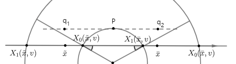
Figure 9. $(\bar{x},v)\in\mathcal{C}_{1}$ and $(\tilde{x},v)\in\mathcal{C}_{2}$.

Let us $v+\zeta=(v_{1},v_{2},v_{3})$. We assume $\zeta=0$ and $v_{2}=0$ without loss of generality, and it is expressed by $v+\zeta=v=(v_{1},0,v_{3})$. For $y:=(y_{1},y_{2},y_{3})$, we classify $y\in A_{1}$ if $R\geq y_{2}>r$, $\bar{x}\in A_{2}$ if $r\geq y_{2}\geq 0$, $\bar{x}\in A_{3}$ if $0>y_{2}\geq-r$, and $y\in A_{4}$ if $-r>y_{2}\geq-R$. (See a Figure 8.)

First, we assume that $\tilde{x},\bar{x}\in A_{1}$. Then we have $(\tilde{x},v),(\bar{x},v)\in\text{$\mathcal{C}_{3}$}$ with moving clockwise, and we get (4.1). Similarly, if $\tilde{x},\bar{x}\in A_{4}$, then $X(s;t,\tilde{x},v)$ and $X(s;t,\bar{x},v)$ are moving counter-clockwise by Remark 2.3. We can reflect $\tilde{x}$, $\bar{x}$ about $x$-axis, then $x,\bar{x}$ belong to $A_{1}$.

Next, assume that $\tilde{x},\bar{x}\in A_{2}$. If $(\tilde{x},v),(\bar{x},v)\in\mathcal{C}_{1}$ or $(\tilde{x},v),(\bar{x},v)\in\mathcal{C}_{2}$, then we have (3.1). We assume that $(\tilde{x},v)\in\text{$\mathcal{C}_{1}$},(\bar{x},v)\in\text{$\mathcal{C}_{2}$}$ with moving clockwise or $(\tilde{x},v)\in\text{$\mathcal{C}_{2}$},(\bar{x},v)\in\text{$\mathcal{C}_{1}$}$ with moving clockwise. (See Figure 9). Let us $p=(0,r,0)+\tilde{x}_{ver}$, $q_{1}=\tilde{x}(\tilde{x}(x,\bar{x},v),p,v)$, and $q_{2}=\tilde{x}(\bar{x},p,v)$. We split

$$\eqref{split2} \leq|f(s,X(s;t,\tilde{x},v),V(s;t,\tilde{x},v))-f(s,X(s;t,q_{1},v),V(s;t,q_{1},v))|$$ (5.8)

$$\quad+|f(s,X(s;t,q_{1},v),V(s;t,q_{1},v))-f(s,X(s;t,p,v),V(s;t,p,v))|$$ (5.9)

$$\quad+|f(s,X(s;t,p,v),V(s;t,p,v))-f(s,X(s;t,q_{2},v),V(s;t,q_{2},v))|$$ (5.10)

$$\quad+|f(s,X(s;t,q_{2},v),V(s;t,q_{2},v))-f(s,X(s;t,\bar{x},v),V(s;t,\bar{x},v))|$$ (5.11)

We apply Lemma 3.1 to (5.9) and (5.10). We apply Lemma 3.5 and Lemma 3.8 to (5.8), (5.11). Because $\cos b(\bar{x},v)=\cos b(\tilde{x},v)$, we obtain (5.6). For $\tilde{x},\bar{x}\in A_{3}$, we also conclude (5.6) since $A_{3}$ and $A_{2}$ are $x$-axial symmetry. ∎

Figure 10. $B_{1},B_{2},B_{3},B_{4}$ and $B_{5}$ for given $v$.

Lemma 5.2.

Fix any point $t,s\in\mathbb{R}^{+}$, $v,\zeta\in\mathbb{R}^{3}$, $x,\bar{x}\in\Omega$. For $\tilde{x}(x,\bar{x},v+\zeta)$ and $|x-\bar{x}|\leq 1$,

$$\begin{split}\frac{\eqref{split1}}{|x-\bar{x}|^{2\beta}}&\lesssim\Big{[}\Big{(}1+|v+\zeta|_{p}(t-s)\Big{)}\mathcal{T}_{sp,1}(x,\tilde{x},v+\zeta)\Big{]}^{2\beta}\\ &\quad\quad\times\Big{[}\frac{e^{\varpi\langle v+\zeta\rangle^{2}s}}{\langle v+\zeta\rangle}\sup_{\begin{subarray}{c}v\in\mathbb{R}^{3}\\ 0<|x-\bar{x}|\leq 1\end{subarray}}\Big{(}e^{-\varpi\langle v\rangle^{2}s}\langle v\rangle\frac{|f(s,x,v)-f(s,\bar{x},v)|}{|x-\bar{x}|^{2\beta}}\Big{)}+\frac{\|wf(s)\|_{\infty}}{w(v+\zeta)}\Big{]}\\ &\quad+\Big{[}\Big{(}|v+\zeta|_{p}+|v+\zeta|_{p}^{2}(t-s)\Big{)}\mathcal{T}_{sp,2}(x,\tilde{x},v+\zeta)\Big{]}^{2\beta}\\ &\quad\quad\times\Big{[}\frac{e^{\varpi\langle v+\zeta\rangle^{2}s}}{\langle v+\zeta\rangle^{2}}\sup_{\begin{subarray}{c}x\in\Omega\\ 0<|v-\bar{v}|\leq 1\end{subarray}}\Big{(}e^{-\varpi\langle v\rangle^{2}s}\langle v\rangle^{2}\frac{|f(s,x,v)-f(s,x,\bar{v})|}{|v-\bar{v}|^{2\beta}}\Big{)}+\frac{\|wf(s)\|_{\infty}}{w(v+\zeta)}\Big{]},\end{split}$$ (5.12)

where $\mathcal{T}_{sp,1}(x,\tilde{x},v+\zeta)$ and $\mathcal{T}_{sp,2}(x,\tilde{x},v+\zeta)$ are defined as

$$\begin{split}\mathcal{T}_{sp,1}(x,\tilde{x},v+\zeta)&=\frac{1}{\cos b(x,v+\zeta)}\mathbf{1}_{\{(x,v+\zeta)\in\text{$\mathcal{C}_{1}$}\}}+\frac{1}{\cos b(x,v+\zeta)}\mathbf{1}_{\{{(x,v+\zeta)}\in\text{$\mathcal{C}_{2}$}\}}\\ &\quad+\frac{1}{\cos b(\tilde{x},v+\zeta)}\mathbf{1}_{\{{(\tilde{x},v+\zeta)}\in\text{$\mathcal{C}_{1}$}\}}+\frac{1}{\cos b(\tilde{x},v+\zeta)}\mathbf{1}_{\{{(\tilde{x},v+\zeta)}\in\text{$\mathcal{C}_{2}$}\}}\\ &\quad+\frac{1}{\cos a(x,v+\zeta)}\mathbf{1}_{\{{(x,v+\zeta)}\in\text{$\mathcal{C}_{3}$}\}}+\frac{1}{\cos a(\tilde{x},v+\zeta)}\mathbf{1}_{\{{(\tilde{x},v+\zeta)}\in\text{$\mathcal{C}_{3}$}\}}\end{split}$$ (5.13)

and

$$\begin{split}\mathcal{T}_{sp,2}(x,\tilde{x},v+\zeta)&=\frac{1}{\cos b(x,v+\zeta)}\mathbf{1}_{\{(x,v+\zeta)\in\text{$\mathcal{C}_{1}$}\}}+\frac{1}{\cos b(x,v+\zeta)}\mathbf{1}_{\{{(x,v+\zeta)}\in\text{$\mathcal{C}_{2}$}\}}\\ &\quad+\frac{1}{\cos b(\tilde{x},v+\zeta)}\mathbf{1}_{\{{(\tilde{x},v+\zeta)}\in\text{$\mathcal{C}_{1}$}\}}+\frac{1}{\cos b(\tilde{x},v+\zeta)}\mathbf{1}_{\{{(\tilde{x},v+\zeta)}\in\text{$\mathcal{C}_{2}$}\}}\\ &\quad+\frac{1}{\cos^{2}a(x,v+\zeta)}\mathbf{1}_{\{{(x,v+\zeta)}\in\text{$\mathcal{C}_{3}$}\}}+\frac{1}{\cos^{2}a(\tilde{x},v+\zeta)}\mathbf{1}_{\{{(\tilde{x},v+\zeta)}\in\text{$\mathcal{C}_{3}$}\}}.\end{split}$$ (5.14)

Here, $b(x,v)$ is in (1.28) or (1.29), and $a(x,v)$ is in (1.30).

Proof.

Let us $v+\zeta=(|v|_{p}\cos\theta_{v},|v|_{p}\sin\theta_{v},v_{3})$. We assume $\zeta=0$ and $\theta_{v}=0$ without loss of generality, and it is expressed by $v+\zeta=v=(v_{1},0,v_{3})$. For given $z=(z_{1},z_{2},z_{3})=(|z|_{p}\cos\theta_{z},|z|_{p}\sin\theta_{z},z_{3})$, we obtain

$$\sin b(z,v)=\frac{|z|_{p}}{r}\sin(\theta_{z}-\theta_{v})=\frac{|z|_{p}}{r}\sin\theta_{z}=\frac{|z_{2}|}{r},\quad b(z,v)\in[0,\pi/2],$$ (5.15)

where $(z,v)\in\mathcal{C}_{1}$ or $\mathcal{C}_{2}$ with moving clockwise by using (2.9). If $(z,v)\in\mathcal{C}_{1}$ or $\mathcal{C}_{2}$ with moving clockwise$(r\geq z_{2}\geq 0)$, then $b(z,v)$ is proportional to $z_{2}$. Similarly,

$$\sin a(z,v)=\frac{|z|_{p}}{R}\sin(\theta_{z}-\theta_{v})=\frac{|z|_{p}}{R}\sin\theta_{z}=\frac{|z_{2}|}{R},\quad a(z,v)\in[0,\pi/2),$$ (5.16)

where $(z,v)\in\mathcal{C}_{3}$ with moving clockwise. Thus if $(z,v)\in\mathcal{C}_{3}$ with moving clockwise$(R\geq z_{2}\geq r)$, then $a(z,v)$ is proportional to $z_{2}$. For $y:=(y_{1},y_{2},y_{3})$, we classify $y\in B_{1}$ if $-r>y_{1}\geq-R$, $y\in B_{2}$ if $0>y_{1}\geq-r$, $y\in B_{3}$ if $y_{1}=0$, $y\in B_{4}$ if $r\geq y_{1}>0$, and $y\in B_{5}$ if $R\geq y_{1}>r$. (See Figure 10.)

Now, let us $x:=(x_{1},x_{2},x_{3})$ and $\tilde{x}:=(\tilde{x}_{1},\tilde{x}_{2},\tilde{x}_{3})$. We split into three cases :
Case 1 First, assume that $x,\tilde{x}\in B_{1}$. If $R\geq x_{2},\tilde{x}_{2}\geq r$, then $(x,v),(\tilde{x},v)\in\text{$\mathcal{C}_{3}$}$ with moving clockwise and we get (5.12) by (4.13). If $R\geq x_{2}\geq r$ and $r\geq\tilde{x}_{2}\geq 0$, then there is $\tau_{+}(x,\bar{x},v)\in[0,1]$ in (3.53). The $(\mathbf{x}(\tau),v)\in\text{$\mathcal{C}_{2}$}$ with moving clockwise for $0\leq\tau\leq\tau_{+}$, and $(\mathbf{x}(\tau),v)\in\text{$\mathcal{C}_{3}$}$ with moving clockwise for $\tau_{+}\leq\tau\leq 1$. We split

$$\quad|f(s,X(s;t,x,v),V(s;t,x,v))-f(s,X(s;t,\tilde{x},v),V(s;t,\tilde{x},v))|$$

$$\leq|f(s,X(s;t,\tilde{x},v),V(s;t,\tilde{x},v))-f(s,X(s;t,\mathbf{x}(\tau_{+}),v),V(s;t,\mathbf{x}(\tau_{+}),v))|$$ (5.17)

$$\quad+|f(s,X(s;t,\mathbf{x}(\tau_{+}),v),V(s;t,\mathbf{x}(\tau_{+}),v))-f(s,X(s;t,x,v),V(s;t,x,v))|.$$ (5.18)

Using (3.54),

$$\Big{|}\int^{\tau_{+}}_{0}\frac{1}{\mathfrak{S}_{sp}(\tau;x,\tilde{x},v)}d\tau\Big{|} \lesssim\Big{(}\frac{1}{|v|_{p}}+\frac{1}{|v|_{p}\cos b(\tilde{x},v)}\Big{)}|\tau_{+}|.$$ (5.19)

From $\sin a(\mathbf{x}(\tau_{+}),v)=r/R$,

$$\text{max}\{\frac{1}{\cos^{2}a(\mathbf{x}(\tau_{+}),v)},\frac{1}{\cos^{2}a(x,v)}\}\lesssim\frac{1}{\cos^{2}a(x,v)},$$ (5.20)

where $a(x,v)$ is in (1.30). We apply (3.34), (5.19) to (5.17), and (4.13),(5.20) to (5.18).
If $r\geq x_{2},\tilde{x}_{2}\geq 0$, then $(\mathbf{x}(\tau),v)\in\text{$\mathcal{C}_{2}$}$ with moving clockwise for $0\leq\tau\leq 1$. From (5.15) and (3.55),

$$\frac{\mathbf{1}_{0\leq\tau\leq 1}}{\mathfrak{S}_{sp}(\tau;x,\tilde{x},v)}\leq\frac{1}{|v|_{p}}\frac{\mathbf{1}_{0\leq\tau\leq 1}}{\cos b(\mathbf{x}(\tau),v)}+\frac{1}{|v|_{p}}\frac{\mathbf{1}_{0\leq\tau\leq 1}}{\cos a(\mathbf{x}(\tau),v)}\lesssim\frac{1}{|v|_{p}}\Big{(}\text{max}\{\frac{1}{\cos b(x,v)},\frac{1}{\cos b(\tilde{x},v)}\}+1\Big{)},$$ (5.21)

where $a(x,v),b(x,v)$ is in (1.29). Using (5.21) and (3.34), we have (5.12).
If $r\geq x_{2}\geq 0$, $0>\tilde{x}_{2}\geq-r$, then there is $\tau_{0}(x,\bar{x},v)\in[0,1]$ in (3.53). The $(\mathbf{x}(\tau),v)\in\text{$\mathcal{C}_{2}$}$ with moving clockwise for $\tau_{0}\leq\tau\leq 1$ and $(\mathbf{x}(\tau),v)\in\text{$\mathcal{C}_{2}$}$ with counter-moving clockwise for $0\leq\tau\leq\tau_{0}$. We split,

$$\quad|f(s,X(s;t,x,v),V(s;t,x,v))-f(s,X(s;t,\tilde{x},v),V(s;t,\tilde{x},v))|$$

$$\leq|f(s,X(s;t,x,v),V(s;t,x,v))-f(s,X(s;t,\mathbf{x}(\tau_{0}),v),V(s;t,\mathbf{x}(\tau_{0}),v))|$$ (5.22)

$$\quad+|f(s,X(s;t,\mathbf{x}(\tau_{0}),v),V(s;t,\mathbf{x}(\tau_{0}),v))-f(s,X(s;t,\tilde{x},v),V(s;t,\tilde{x},v))|.$$ (5.23)

Using (3.55), (5.15), and $\cos b(\mathbf{x}(\tau_{0}),v)=1$,

$$\frac{\mathbf{1}_{\tau_{0}\leq\tau\leq 1}}{\mathfrak{S}_{sp}(\tau;x,\tilde{x},v)}\lesssim\frac{1}{|v|_{p}}\Big{(}\frac{1}{\cos b(x,v)}+1\Big{)},$$ (5.24)

and

$$\frac{\mathbf{1}_{0\leq\tau\leq\tau_{0}}}{\mathfrak{S}_{sp}(\tau;x,\tilde{x},v)}\lesssim\frac{1}{|v|_{p}}\Big{(}\frac{1}{\cos b(\tilde{x},v)}+1\Big{)},$$ (5.25)

where $b(x,v)$ is in (1.29). For $\tau_{0}\leq\tau\leq 1$, we apply (3.34), (5.24) to (5.22). For $0\leq\tau\leq\tau_{0}$, we apply (3.34), (5.25) to (5.23) after reflecting $X(s;t,\mathbf{x}(\tau),v)$ about x-axis.
If $R\geq x_{2}\geq r$, $0>\tilde{x}_{2}\geq-r$, then there is $\tau_{0}(x,\bar{x},v),\tau_{+}(x,\bar{x},v)\in[0,1]$ in (3.53). The $(\mathbf{x}(\tau),v)\in\text{$\mathcal{C}_{2}$}$ with counter-moving clockwise for $0\leq\tau\leq\tau_{0}$, and $(\mathbf{x}(\tau),v)\in\text{$\mathcal{C}_{2}$}$ with moving clockwise for $\tau_{0}\leq\tau\leq\tau_{+}$, and $(\mathbf{x}(\tau),v)\in\text{$\mathcal{C}_{3}$}$ with moving clockwise for $\tau_{+}\leq\tau\leq 1$. We split,

$$\quad|f(s,X(s;t,x,v),V(s;t,x,v))-f(s,X(s;t,\tilde{x},v),V(s;t,\tilde{x},v))|$$

$$\leq|f(s,X(s;t,x,v),V(s;t,x,v))-f(s,X(s;t,\mathbf{x}(\tau_{+}),v),V(s;t,\mathbf{x}(\tau_{+}),v))|$$ (5.26)

$$\quad+|f(s,X(s;t,\mathbf{x}(\tau_{+}),v),V(s;t,\mathbf{x}(\tau_{+}),v))-f(s,X(s;t,\mathbf{x}(\tau_{0}),v),V(s;t,\mathbf{x}(\tau_{0}),v))|.$$ (5.27)

$$\quad+|f(s,X(s;t,\mathbf{x}(\tau_{0}),v),V(s;t,\mathbf{x}(\tau_{0}),v))-f(s,X(s;t,\tilde{x},v),V(s;t,\tilde{x},v))|.$$ (5.28)

We apply (5.20), (4.18) to (5.26). Using (3.54) and $\cos b(\mathbf{x}(\tau_{0}),v)=1$,

$$\Big{|}\int^{\tau_{+}}_{\tau_{0}}\frac{1}{\mathfrak{S}_{sp}(\tau;x,\tilde{x},v)}d\tau\Big{|} \lesssim\Big{(}\frac{1}{|v|_{p}}+\frac{1}{|v|_{p}\cos b(\mathbf{x}(\tau_{0}),v)}\Big{)}|\tau_{+}-\tau_{0}|\lesssim\frac{1}{|v|_{p}}$$ (5.29)

and we apply (5.29), (3.34) to (5.27). After reflecting $X(s;t,\mathbf{x}(\tau),v)$ for $0\leq\tau\leq\tau_{0}$, we apply (5.25), (3.34) to (5.28).
If $R\geq x_{2}\geq r$, $-r\geq\tilde{x}_{2}\geq-R$, then there is $\tau_{0}(x,\bar{x},v)\in[0,1]$ in (3.53). The $X(s;t,\mathbf{x}(\tau),v)$ moves with counter-clockwise for $0\leq\tau\leq\tau_{0}$. After reflecting $X(s;t,\mathbf{x}(\tau),v)$ about x-axis, we use same arguments to (5.26), (5.27). The $X(s;t,\mathbf{x}(\tau),v)$ moves with clockwise for $\tau_{0}\leq\tau\leq 1$, and we use (5.26),(5.27) directly.

Case 2 Second, we assume $x,\tilde{x}\in B_{2}$. If $R\geq x_{2},\tilde{x}_{2}\geq r$ or $R\geq x_{2}\geq r,r\geq\tilde{x}_{2}\geq 0$ or $r\geq x_{2},\tilde{x}_{2}\geq 0$, then we can use same arguments to $x,\tilde{x}\in B_{1}$. Next, we assume that $r\geq x_{2}\geq 0$, $0\geq\tilde{x}_{2}\geq-r$ or $R\geq x_{2}\geq r$, $0\geq\tilde{x}_{2}\geq-r$ or $R\geq x_{2}\geq r$, $-r\geq\tilde{x}_{2}\geq-R$. Define

$$p(x,v)=x\mathbf{1}_{0\leq x_{2}\leq r}+\mathbf{x}(\tau_{+})\mathbf{1}_{r<x_{2}\leq R}=(p_{1}(x,v),p_{2}(x,v),p_{3}(x,v)),$$

$$q(\tilde{x},v)=\tilde{x}\mathbf{1}_{-r\leq\tilde{x}_{2}\leq 0}+\mathbf{x}(\tau_{-})\mathbf{1}_{-R<\tilde{x}_{2}\leq-r}=(q_{1}(\tilde{x},v),q_{2}(\tilde{x},v),q_{3}(\tilde{x},v)).$$

Here, $\tau_{+}(x,\bar{x},v)$ is in (3.53), and $\tau_{-}(x,\bar{x},v)$ satisfies $\hat{v}_{p}\cdot n(X_{0}(\mathbf{x}(\tau_{-}),v))=0$. There is $\alpha_{*}\in\mathbb{R}^{+}$ such that $-r>p_{1}(x,v)-\alpha_{*}v_{1}>-R$, $-r>q_{1}(\tilde{x},v)-\alpha_{*}v_{1}>-R$, and $|\alpha_{*}v_{1}|\leq|x-\tilde{x}|$. Let us

$$p_{*}(x,v)=(p_{1}(x,v)-\alpha_{*}v_{1},v_{2},v_{3})\text{ \;and \;}q_{*}(\tilde{x},v)=(q_{1}(\tilde{x},v)-\alpha_{*}v_{1},v_{2},v_{3}).$$

Then we have

$$b(p(x,v),v)=b(p_{*}(x,v),v)\text{ \;and \;}b(q(\tilde{x},v),v)=b(q_{*}(\tilde{x},v),v),$$

where $b(x,v)$ in (1.29). We can split

$$\quad|f(s,X(s;t,x,v),V(s;t,x,v))-f(s,X(s;t,\tilde{x},v),V(s;t,\tilde{x},v))|$$

$$\leq|f(s,X(s;t,x,v),V(s;t,x,v))-f(s,X(s;t,p(x,v),v),V(s;t,p(x,v),v))|$$ (5.30)

$$\quad+|f(s,X(s;t,p(x,v),v),V(s;t,p(x,v),v))-f(s,X(s;t,p_{*}(x,v),v),V(s;t,p_{*}(x,v),v))|$$ (5.31)

$$\quad+|f(s,X(s;t,p_{*}(x,v),v),V(s;t,p_{*}(x,v),v))-f(s,X(s;t,q_{*}(\tilde{x},v),v),V(s;t,q_{*}(\tilde{x},v),v))|$$ (5.32)

$$\quad+|f(s,X(s;t,q_{*}(\tilde{x},v),v),V(s;t,q_{*}(\tilde{x},v),v))-f(s,X(s;t,q(\tilde{x},v),v),V(s;t,q(\tilde{x},v),v))|$$ (5.33)

$$\quad+|f(s,X(s;t,q(\tilde{x},v),v),V(s;t,q(\tilde{x},v),v))-f(s,X(s;t,\tilde{x},v),V(s;t,\tilde{x},v))|.$$ (5.34)

We apply (4.13), (5.20) to (5.30), (5.34), and (3.1) to (5.31), (5.33). Because $p_{*}(x,v),q_{*}(\tilde{x},v)\in B_{1}$, we obtain (5.12).

Case 3 Lastly, we assume $x,\tilde{x}\in B_{3}$. If $R\geq x_{2},\tilde{x}_{2}\geq r$, then $(x,v),(\tilde{x},v)\in\text{$\mathcal{C}_{3}$}$ with moving clockwise, and it is same as $x,\tilde{x}\in B_{1}$. If $-r\geq x_{2},\tilde{x}_{2}\geq-R$, then we reflect $X(s;t,x,v)$ and $X(s;t,\tilde{x},v)$ about $x$-axis. If $R\geq x_{2}\geq r$, $-r\geq x_{2}\geq-R$, we use same same arguments when $x_{2},\tilde{x}_{2}\in B_{2}$. Lastly, assume $x,\tilde{x}\in B_{4}$ or $x,\tilde{x}\in B_{5}$. Then we consider $\mathcal{C}_{1}$ instead of $\mathcal{C}_{2}$ in above, and omit details. Therefore, we conclude (5.12) for any $x,\bar{x}\in\Omega$ when $v\in\mathbb{R}^{3}$ is fixed. ∎

Lemma 5.3.

Fix any point $t,s\in\mathbb{R}^{+}$, $v,\bar{v},\zeta\in\mathbb{R}^{3}$, $\bar{x}\in\Omega$. For $\tilde{v}(v,\bar{v},\zeta)$,

$$\begin{split}\frac{\eqref{split4}}{|v-\bar{v}|^{2\beta}}&\lesssim\Big{[}(t-s)+\text{max}\{\frac{1}{|v+\zeta|_{p}},\frac{1}{|\bar{v}+\zeta|_{p}}\}\Big{]}^{2\beta}\\ &\quad\quad\times\Big{[}\frac{e^{\varpi\langle v+\zeta\rangle^{2}s}}{\langle v+\zeta\rangle}\sup_{\begin{subarray}{c}v\in\mathbb{R}^{3}\\ 0<|x-\bar{x}|\leq 1\end{subarray}}\Big{(}e^{-\varpi\langle v\rangle^{2}s}\langle v\rangle\frac{|f(s,x,v)-f(s,\bar{x},v)|}{|x-\bar{x}|^{2\beta}}\Big{)}+\frac{\|wf(s)\|_{\infty}}{w(v+\zeta)}\Big{]}\\ &\quad+\Big{[}1+(t-s)\text{max}\{|v+\zeta|_{p},|\bar{v}+\zeta|_{p}\}\Big{]}^{2\beta}\\ &\quad\quad\times\Big{[}\frac{e^{\varpi\langle v+\zeta\rangle^{2}s}}{\langle v+\zeta\rangle^{2}}\sup_{\begin{subarray}{c}x\in\Omega\\ 0<|v-\bar{v}|\leq 1\end{subarray}}\Big{(}e^{-\varpi\langle v\rangle^{2}s}\langle v\rangle^{2}\frac{|f(s,x,v)-f(s,x,\bar{v})|}{|v-\bar{v}|^{2\beta}}\Big{)}+\frac{\|wf(s)\|_{\infty}}{w(v+\zeta)}\Big{]}.\end{split}$$ (5.35)

Proof.

Because $(\bar{x},\tilde{v}+\zeta),(\bar{x},\bar{v}+\zeta)\in\text{$\mathcal{C}_{1}$}$ or $(\bar{x},\tilde{v}+\zeta),(\bar{x},\bar{v}+\zeta)\in\text{$\mathcal{C}_{2}$}$ or $(\bar{x},\tilde{v}+\zeta),(\bar{x},\bar{v}+\zeta)\in\text{$\mathcal{C}_{3}$}$, we obtain (5.35) from Lemma 3.2 and Lemma 4.2. ∎

Lemma 5.4.

Fix any point $t,s\in\mathbb{R}^{+}$, $v,\bar{v},\zeta\in\mathbb{R}^{3}$, $\bar{x}\in\Omega$. For $\tilde{v}(v,\bar{v},\zeta)$,

$$\begin{split}\frac{\eqref{split3}}{|v-\bar{v}|^{2\beta}}&\lesssim\Big{[}\Big{(}\frac{1}{|v+\zeta|_{p}}+(t-s)\Big{)}\Big{]}^{2\beta}\\ &\quad\quad\times\Big{[}\frac{e^{\varpi\langle v+\zeta\rangle^{2}s}}{\langle v+\zeta\rangle}\sup_{\begin{subarray}{c}v\in\mathbb{R}^{3}\\ 0<|x-\bar{x}|\leq 1\end{subarray}}\Big{(}e^{-\varpi\langle v\rangle^{2}s}\langle v\rangle\frac{|f(s,x,v)-f(s,\bar{x},v)|}{|x-\bar{x}|^{2\beta}}\Big{)}+\frac{\|wf(s)\|_{\infty}}{w(v+\zeta)}\Big{]}\\ &\quad+\Big{[}\Big{(}1+|v+\zeta|_{p}(t-s)\Big{)}\mathcal{T}_{vel}(\bar{x},v,\tilde{v},\zeta)\Big{]}^{2\beta}\\ &\quad\quad\times\Big{[}\frac{e^{\varpi\langle v+\zeta\rangle^{2}s}}{\langle v+\zeta\rangle^{2}}\sup_{\begin{subarray}{c}x\in\Omega\\ 0<|v-\bar{v}|\leq 1\end{subarray}}\Big{(}e^{-\varpi\langle v\rangle^{2}s}\langle v\rangle^{2}\frac{|f(s,x,v)-f(s,x,\bar{v})|}{|v-\bar{v}|^{2\beta}}\Big{)}+\frac{\|wf(s)\|_{\infty}}{w(v+\zeta)}\Big{]},\end{split}$$ (5.36)

where $\mathcal{T}_{vel}(\bar{x},v,\tilde{v},\zeta)$ is defined as

$$\begin{split}\mathcal{T}_{vel}(\bar{x},v,\tilde{v},\zeta)&=\frac{1}{\cos b(\bar{x},v+\zeta)}\mathbf{1}_{\{{(\bar{x},v+\zeta)}\in\text{$\mathcal{C}_{1}$}\}}+\frac{1}{\cos b(\bar{x},v+\zeta)}\mathbf{1}_{\{{(\bar{x},v+\zeta)}\in\text{$\mathcal{C}_{2}$}\}}\\ &\quad+\frac{1}{\cos b(\bar{x},\tilde{v}+\zeta)}\mathbf{1}_{\{{(\bar{x},\tilde{v}+\zeta)}\in\text{$\mathcal{C}_{1}$}\}}+\frac{1}{\cos b(\bar{x},\tilde{v}+\zeta)}\mathbf{1}_{\{{(\bar{x},\tilde{v}+\zeta)}\in\text{$\mathcal{C}_{2}$}\}}\\ &\quad+\frac{1}{\cos a(\bar{x},v+\zeta)}\mathbf{1}_{\{{(\bar{x},v+\zeta)}\in\text{$\mathcal{C}_{3}$}\}}+\frac{1}{\cos a(\bar{x},\tilde{v}+\zeta)}\mathbf{1}_{\{{(\bar{x},\tilde{v}+\zeta)}\in\text{$\mathcal{C}_{3}$}\}}.\end{split}$$ (5.37)

Here, $b(x,v)$ is in (1.28) or (1.29), and $a(x,v)$ is in (1.30).

Proof.

Let $\bar{x}=(x_{1},x_{2},x_{3})=(|x|_{p}\cos\theta_{x},|x|_{p}\sin\theta_{x},x_{3})$. We assume $x_{1}=0$ and $x_{2}>0$ without loss of generality. For $w=(|w|_{p}\cos\theta_{w},|w|_{p}\sin\theta_{w},w_{3})$, we recall (2.9)

$$\sin b(\bar{x},w)=\frac{|x|_{p}}{r}\sin(\theta_{x}-\theta_{w})=\frac{|x|_{p}}{r}\cos\theta_{w}.$$ (5.38)

Let $\theta_{*}=\sin^{-1}(r/x_{2})\in[0,\pi/2]$. For $w=(|w|_{p}\cos\theta_{w},|w|_{p}\sin\theta_{w},w_{3})$, we classify $w\in D_{1}$ if $-\pi/2\leq\theta_{w}\leq-\pi/2+\theta_{*}$, and $w\in D_{2}$ if $-\pi/2+\theta_{*}\leq\theta_{w}\leq\pi/2-\theta_{*}$, and $w\in D_{3}$ if $\pi/2-\theta_{*}\leq\theta_{w}\leq\pi/2$, and $w\in D_{4}$ if $\pi/2\leq\theta_{w}\leq\pi/2+\theta_{*}$, and $w\in D_{5}$ if $\pi/2+\theta_{*}\leq\theta_{w}\leq\pi$ or $-\pi\leq\theta_{w}\leq-\pi/2-\theta_{*}$, and $w\in D_{6}$ if $-\pi/2-\theta_{*}\leq\theta_{w}\leq-\pi/2$. (See Figure 11.) Then $(\bar{x},w)\in\text{$\mathcal{C}_{2}$}$ with moving clockwise if $w\in D_{1}$, and $(\bar{x},w)\in\text{$\mathcal{C}_{3}$}$ with moving clockwise if $w\in D_{2}$, and $(\bar{x},w)\in\text{$\mathcal{C}_{1}$}$ with moving clockwise if $w\in D_{3}$, and $(\bar{x},w)\in\text{$\mathcal{C}_{1}$}$ with moving counter-clockwise if $w\in D_{4}$, and $(\bar{x},w)\in\text{$\mathcal{C}_{3}$}$ with moving counter-clockwise if $w\in D_{5}$, and $(\bar{x},w)\in\text{$\mathcal{C}_{2}$}$ with moving counter-clockwise if $w\in D_{6}$.

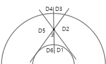
Figure 11. $D_{1},D_{2},D_{3},D_{4},D_{5}$ and $D_{6}$ for given $\bar{x}$.

Let $v+\zeta=(|v|_{p}\cos\theta_{v},|v|_{p}\sin\theta_{v},v_{3})$ and $\tilde{v}+\zeta=(|v|_{p}\cos\theta_{\tilde{v}},|v|_{p}\sin\theta_{\tilde{v}},v_{3})$ for $\theta_{v},\theta_{\tilde{v}}\in[-\pi,\pi]$, and assume $x_{2}\neq r$. Now, we split into four cases :

Case 1 First, assume that both $v+\zeta,\;\tilde{v}+\zeta\in D_{1}$. Then $(\bar{x},\mathbf{v}(\tau))\in\mathcal{C}_{2}$ with moving clockwise for $0\leq\tau\leq 1$. For $\mathbf{v}(\tau),\Theta(\tau)$ in (1.37), we have

$$-\frac{\pi}{2}\leq\text{min}\{\theta_{v},\theta_{\tilde{v}}\}\leq\Theta(\tau)\leq\text{max}\{\theta_{v},\theta_{\tilde{v}}\}\leq-\frac{\pi}{2}+\theta_{*}$$

and

$$\text{max}_{0\leq\tau\leq 1}\cos\Theta(\tau)=\text{max}\{\cos\theta_{v},\cos\theta_{\tilde{v}}\}.$$ (5.39)

Applying (5.39) to (5.38),

$$\text{max}_{0\leq\tau\leq 1}\sin b(\bar{x},\mathbf{v}(\tau))=\text{max}\{\sin b(\bar{x},v+\zeta),\sin b(\bar{x},\tilde{v}+\zeta)\}$$

and

$$\text{max}_{0\leq\tau\leq 1}\{\frac{1}{\cos b(\bar{x},\mathbf{v}(\tau))}\}=\text{max}\{\frac{1}{\cos b(\bar{x},v+\zeta)},\frac{1}{\cos b(\bar{x},\tilde{v}+\zeta)}\}$$

since $b(x,v)\in[0,\pi/2]$. By (3.55) and $t_{*}(\bar{x},v)\lesssim 1/|v|_{p}$,

$$\begin{split}\frac{\mathbf{1}_{0\leq\tau\leq 1}}{\mathfrak{S}_{vel}(\tau;\bar{x},v,\tilde{v},\zeta)}&\leq\frac{t_{b}(\bar{x},\mathbf{v}(\tau))\mathbf{1}_{0\leq\tau\leq 1}}{|v+\zeta|_{p}\cos a(\bar{x},\mathbf{v}(\tau))}+\frac{t_{f}(\bar{x},\mathbf{v}(\tau))\mathbf{1}_{0\leq\tau\leq 1}}{|v+\zeta|_{p}\cos b(\bar{x},\mathbf{v}(\tau))}\\ &\lesssim\frac{1}{|v+\zeta|^{2}_{p}}\Big{(}1+\text{max}\{\frac{1}{\cos b(\bar{x},v+\zeta)},\frac{1}{\cos b(\bar{x},\tilde{v}+\zeta)}\}\Big{)}.\end{split}$$ (5.40)

Here, $a(x,v),b(x,v)$ are in (1.29). We apply (5.40) to (3.44), and get (5.36). We can use same arguments when $v+\zeta,\;\tilde{v}+\zeta$ are located in $D_{3}$. Next, assume that both $v+\zeta,\;\tilde{v}+\zeta\in D_{2}$. Then $(\bar{x},v+\zeta),(\bar{x},\tilde{v}+\zeta)\in\mathcal{C}_{3}$ with moving clockwise, and we get (5.36) from (4.18) directly. If both $v+\zeta,\tilde{v}+\zeta\in D_{4}$ or $v+\zeta,\tilde{v}+\zeta\in D_{5}$ or $v+\zeta,\tilde{v}+\zeta\in D_{6}$, then we reflect $v+\zeta,\;\tilde{v}+\zeta$ about y-axis.

Case 2 Second, we assume that $\tilde{v}+\zeta\in D_{1}$, and $v+\zeta\in D_{2}$. Then there is $\tau_{-}(\bar{x},v,\bar{v},\zeta)\in[0,1]$ in (3.59). The $(\bar{x},\mathbf{v}(\tau))\in\mathcal{C}_{2}$ with moving clockwise for $0\leq\tau\leq\tau_{-}$, and $(\bar{x},\mathbf{v}(\tau))\in\mathcal{C}_{3}$ with moving clockwise for $\tau_{-}\leq\tau\leq 1$. We can split

$$\quad|f(s,X(s;t,\bar{x},\tilde{v}+\zeta),V(s;t,\bar{x},\tilde{v}+\zeta))-f(s,X(s;t,\bar{x},v+\zeta),V(s;t,\bar{x},v+\zeta))|$$

$$\leq|f(s,X(s;t,\bar{x},\tilde{v}+\zeta),V(s;t,\bar{x},\tilde{v}+\zeta))-f(s,X(s;t,\bar{x},\mathbf{v}(\tau_{-})),V(s;t,\bar{x},\mathbf{v}(\tau_{-})))|$$ (5.41)

$$\quad+|f(s,X(s;t,\bar{x},\mathbf{v}(\tau_{-})),V(s;t,\bar{x},\mathbf{v}(\tau_{-})))-f(s,X(s;t,\bar{x},v+\zeta),V(s;t,\bar{x},v+\zeta))|.$$ (5.42)

Because $\cos a(\bar{x},\mathbf{v}(\tau_{-}))=\sqrt{1-(r/R)^{2}}$ for $a(x,v)$ in (1.30),

$$\text{max}\{{\frac{1}{\cos a(\bar{x},\mathbf{v}(\tau_{-}))},\frac{1}{\cos a(\bar{x},v+\zeta)}}\}\lesssim\frac{1}{\cos a(\bar{x},v+\zeta)}.$$ (5.43)

We apply (3.44),(3.61) to (5.41), and (4.18), (5.43) to (5.42). Then we get (5.36). If $\tilde{v}+\zeta\in{D_{5}}$ and $v+\zeta\in{D_{6}}$, then we reflect $v+\zeta,\;\tilde{v}+\zeta$ about y-axis. If $\tilde{v}+\zeta\in D_{2},v+\zeta\in D_{3}$ or $\tilde{v}+\zeta\in D_{5},v+\zeta\in D_{4}$, we consider $\mathcal{C}_{1}$ instead of $\mathcal{C}_{2}$ in above.
Assume that $\tilde{v}+\zeta\in D_{6}$ and $v+\zeta\in D_{1}$. Then there is $\tau_{0-}(\bar{x},v,\bar{v},\zeta)\in[0,1]$ in (3.59). The $(\bar{x},\mathbf{v}(\tau))\in\text{$\mathcal{C}_{2}$}$ with moving counter-clockwise for $0\leq\tau\leq\tau_{0-}$, and $(\bar{x},\mathbf{v}(\tau))\in\text{$\mathcal{C}_{2}$}$ with moving clockwise for $\tau_{0-}\leq\tau\leq 1$. We split

$$\quad|f(s,X(s;t,\bar{x},\tilde{v}+\zeta),V(s;t,\bar{x},\tilde{v}+\zeta))-f(s,X(s;t,\bar{x},v+\zeta),V(s;t,\bar{x},v+\zeta))|$$

$$\leq|f(s,X(s;t,\bar{x},\tilde{v}+\zeta),V(s;t,\bar{x},\tilde{v}+\zeta))-f(s,X(s;t,\bar{x},\mathbf{v}(\tau_{0-})),V(s;t,\bar{x},\mathbf{v}(\tau_{0-})))|$$ (5.44)

$$\quad+|f(s,X(s;t,\bar{x},\mathbf{v}(\tau_{0-})),V(s;t,\bar{x},\mathbf{v}(\tau_{0-})))-f(s,X(s;t,\bar{x},v+\zeta),V(s;t,\bar{x},v+\zeta))|.$$ (5.45)

For $\tau_{0-}\leq\tau\leq 1$,

$$-\pi/2\leq\Theta(\tau)\leq\theta_{v}\leq-\pi/2+\theta_{*}$$

and

$$\text{max}_{\tau_{0-}\leq\tau\leq 1}\cos\Theta(\tau)=\cos\theta_{v}.$$

By (5.38),

$$\text{max}_{\tau_{0-}\leq\tau\leq 1}\sin b(\bar{x},\mathbf{v}(\tau))=\sin b(\bar{x},v+\zeta)$$

and

$$\text{max}_{\tau_{0-}\leq\tau\leq 1}\frac{1}{\cos b(\bar{x},\mathbf{v}(\tau))}=\frac{1}{\cos b(\bar{x},v+\zeta)}$$

since $b(x,v)\in[0,\pi/2]$. By (3.55) and $t_{*}(\bar{x},v)\lesssim 1/|v|_{p}$,

$$\frac{\mathbf{1}_{\tau_{0-}\leq\tau\leq 1}}{\mathfrak{S}_{vel}(\tau;\bar{x},v,\tilde{v},\zeta)} \leq\frac{t_{b}(\bar{x},\mathbf{v}(\tau))\mathbf{1}_{\tau_{0-}\leq\tau\leq 1}}{|v+\zeta|_{p}\cos a(\bar{x},\mathbf{v}(\tau))}+\frac{t_{f}(\bar{x},\mathbf{v}(\tau))\mathbf{1}_{\tau_{0-}\leq\tau\leq 1}}{|v+\zeta|_{p}\cos b(\bar{x},\mathbf{v}(\tau))}$$

$$\lesssim\frac{1}{|v+\zeta|^{2}_{p}}(1+\frac{1}{\cos b(\bar{x},v+\zeta)}).$$ (5.46)

We reflect $X(s;t,\bar{x},\mathbf{v}(\tau))$ about y-axis for $0\leq\tau\leq\tau_{0-}$. Then similar to (5.1),

$$\frac{\mathbf{1}_{0\leq\tau\leq\tau_{0-}}}{\mathfrak{S}_{vel}(\tau;\bar{x},v,\tilde{v},\zeta)} \leq\frac{t_{b}(\bar{x},\mathbf{v}(\tau))\mathbf{1}_{0\leq\tau\leq\tau_{0-}}}{|v+\zeta|_{p}\cos a(\bar{x},\mathbf{v}(\tau))}+\frac{t_{f}(\bar{x},\mathbf{v}(\tau))\mathbf{1}_{0\leq\tau\leq\tau_{0-}}}{|v+\zeta|_{p}\cos b(\bar{x},\mathbf{v}(\tau))}$$

$$\lesssim\frac{1}{|v+\zeta|^{2}_{p}}\Big{(}1+\frac{1}{\cos b(\bar{x},\tilde{v}+\zeta)}\Big{)}.$$ (5.47)

We apply (3.44), (5.1) to (5.44) and (3.44), (5.1) to (5.45). Then we get (5.36). If $\tilde{v}+\zeta\in D_{3}$ and $v+\zeta\in D_{4}$, we can use same arguments above.

Case 3 Assume $\tilde{v}+\zeta\in D_{1}$ and $v+\zeta\in D_{3}$. There are $\tau_{-}(\bar{x},v,\bar{v},\zeta)\in[0,1]$ in (3.59) and $\tau_{+}(\bar{x},v,\bar{v},\zeta)\in[0,1]$ in (3.58), and it holds that $0\leq\tau_{-}(\bar{x},v,\bar{v},\zeta)\leq\tau_{+}(\bar{x},v,\bar{v},\zeta)\leq 1$. The $(\bar{x},\mathbf{v}(\tau))\in\text{$\mathcal{C}_{2}$}$ with moving clockwise for $0\leq\tau\leq\tau_{-}$, and $(\bar{x},\mathbf{v}(\tau))\in\text{$\mathcal{C}_{3}$}$ with moving clockwise for $\tau_{-}\leq\tau\leq\tau_{+}$, and $(\bar{x},\mathbf{v}(\tau))\in\text{$\mathcal{C}_{1}$}$ with moving clockwise for $\tau_{+}\leq\tau\leq 1$. We split

$$\quad|f(s,X(s;t,\bar{x},\tilde{v}+\zeta),V(s;t,\bar{x},\tilde{v}+\zeta))-f(s,X(s;t,\bar{x},v+\zeta),V(s;t,\bar{x},v+\zeta))|$$

$$\leq|f(s,X(s;t,\bar{x},\tilde{v}+\zeta),V(s;t,\bar{x},\tilde{v}+\zeta))-f(s,X(s;t,\bar{x},\mathbf{v}(\tau_{-})),V(s;t,\bar{x},\mathbf{v}(\tau_{-})))|$$ (5.48)

$$\quad+|f(s,X(s;t,\bar{x},\mathbf{v}(\tau_{-})),V(s;t,\bar{x},\mathbf{v}(\tau_{-})))-f(s,X(s;t,\bar{x},\mathbf{v}(\tau_{+})),V(s;t,\bar{x},\mathbf{v}(\tau_{+})))|$$ (5.49)

$$\quad+|f(s,X(s;t,\bar{x},\mathbf{v}(\tau_{+})),V(s;t,\bar{x},\mathbf{v}(\tau_{+})))-f(s,X(s;t,\bar{x},v+\zeta),V(s;t,\bar{x},v+\zeta))|.$$ (5.50)

From (3.61),

$$\Big{|}\int^{\tau_{-}}_{0}\frac{1}{\mathfrak{S}_{vel}(\tau;\bar{x},v,\tilde{v},\zeta)}d\tau\Big{|}\lesssim\Big{(}\frac{1}{|v+\zeta|^{2}_{p}}+\frac{1}{\cos b(\bar{x},\tilde{v}+\zeta)}\frac{1}{|v+\zeta|^{2}_{p}}\Big{)}|\tau_{-}|,$$ (5.51)

where $b(x,v)$ is in (1.29). From (3.60),

$$\Big{|}\int^{1}_{\tau_{+}}\frac{1}{\mathfrak{S}_{vel}(\tau;\bar{x},v,\tilde{v},\zeta)}d\tau\Big{|}\lesssim\Big{(}\frac{1}{|v+\zeta|^{2}_{p}}+\frac{1}{\cos b(\bar{x},v+\zeta))}\frac{1}{|v+\zeta|^{2}_{p}}\Big{)}|1-\tau_{+}|,$$ (5.52)

where $b(x,v)$ is in (1.28). Because $\sin(\bar{x},\mathbf{v}(\tau_{-}))=\sin(\bar{x},\mathbf{v}(\tau_{+}))=r/R$,

$$\text{max}\{\frac{1}{\cos^{2}a(\bar{x},\mathbf{v}(\tau_{-}))},\frac{1}{\cos^{2}a(\bar{x},\mathbf{v}(\tau_{+}))}\}\lesssim 1,$$ (5.53)

where $a(x,v)$ is in (1.30). We apply (3.44), (5.51) to (5.48) and (4.18), (5.53) to (5.49). We also apply (3.44), (5.52) to (5.50), and we get (5.36). If $\tilde{v}+\zeta\in{D_{4}}$ and $v+\zeta\in{D_{6}}$, then we reflect $v+\zeta,\;\tilde{v}+\zeta$ about y-axis. If $\tilde{v}+\zeta\in D_{2}$ and $v+\zeta\in D_{4}$, there are $\tau_{+}(\bar{x},v,\bar{v},\zeta)$ and $\tau_{0+}(\bar{x},v,\bar{v},\zeta)\in[0,1]$ in (3.58) for $0\leq\tau_{+}(\bar{x},v,\bar{v},\zeta)\leq\tau_{0+}(\bar{x},v,\bar{v},\zeta)\leq 1$. The $(\bar{x},\mathbf{v}(\tau))\in\text{$\mathcal{C}_{3}$}$ with moving clockwise for $0\leq\tau\leq\tau_{+}$, $(\bar{x},\mathbf{v}(\tau))\in\text{$\mathcal{C}_{1}$}$ with moving clockwise for $\tau_{+}\leq\tau\leq\tau_{0+}$ and $(x,\mathbf{v}(\tau))\in\text{$\mathcal{C}_{1}$}$ with counter-moving clockwise for $\tau_{0+}\leq\tau\leq 1$. We split

$$\quad|f(s,X(s;t,\bar{x},\tilde{v}+\zeta),V(s;t,\bar{x},\tilde{v}+\zeta))-f(s,X(s;t,\bar{x},v+\zeta),V(s;t,\bar{x},v+\zeta))|$$

$$\leq|f(s,X(s;t,\bar{x},\tilde{v}+\zeta),V(s;t,\bar{x},\tilde{v}+\zeta))-f(s,X(s;t,\bar{x},\mathbf{v}(\tau_{+})),V(s;t,\bar{x},\mathbf{v}(\tau_{+})))|$$ (5.54)

$$\quad+|f(s,X(s;t,\bar{x},\mathbf{v}(\tau_{+})),V(s;t,\bar{x},\mathbf{v}(\tau_{+})))-f(s,X(s;t,\bar{x},\mathbf{v}(\tau_{0+})),V(s;t,\bar{x},\mathbf{v}(\tau_{0+})))|$$ (5.55)

$$\quad+|f(s,X(s;t,\bar{x},\mathbf{v}(\tau_{0+})),V(s;t,\bar{x},\mathbf{v}(\tau_{0+})))-f(s,X(s;t,\bar{x},v+\zeta),V(s;t,\bar{x},v+\zeta))|.$$ (5.56)

From $\sin a(\bar{x},\mathbf{v}(\tau_{+}))=r/R$,

$$\text{max}\{\frac{1}{\cos a(\bar{x},\mathbf{v}(\tau_{+}))},\frac{1}{\cos a(\bar{x},\tilde{v}+\zeta)}\}\lesssim\frac{1}{\cos a(\bar{x},\tilde{v}+\zeta)},$$ (5.57)

where $a(x,v)$ is in (1.30). Using $\cos(\bar{x},\mathbf{v}(\tau_{0+}))=1$ and (3.60),

$$\begin{split}\Big{|}\int^{\tau_{0+}}_{\tau_{+}}\frac{1}{\mathfrak{S}_{vel}(\tau;x,v,\tilde{v},\zeta)}d\tau\Big{|}&\lesssim\Big{(}\frac{1}{|v+\zeta|^{2}_{p}}+\frac{1}{\cos b(x,\mathbf{v}(\tau_{0+}))}\frac{1}{|v+\zeta|^{2}_{p}}\Big{)}|\tau_{0+}-\tau_{+}|\lesssim\frac{1}{|v+\zeta|^{2}_{p}},\end{split}$$ (5.58)

where $b(x,v)$ is in (1.28). After reflecting $X(s;t,\bar{x},\mathbf{v}(\tau))$ about y-axis for $\tau_{0+}\leq\tau\leq 1$, we use (3.55) and (5.38). Then we get

$$\frac{\mathbf{1}_{\tau_{0+}\leq\tau\leq 1}}{\mathfrak{S}_{vel}(\tau;\bar{x},v,\tilde{v},\zeta)} \leq\frac{t_{b}(\bar{x},\mathbf{v}(\tau))\mathbf{1}_{\tau_{0+}\leq\tau\leq 1}}{|v+\zeta|_{p}\cos a(\bar{x},\mathbf{v}(\tau))}+\frac{t_{f}(\bar{x},\mathbf{v}(\tau))\mathbf{1}_{\tau_{0+}\leq\tau\leq 1}}{|v+\zeta|_{p}\cos b(\bar{x},\mathbf{v}(\tau))}$$

$$\lesssim\frac{1}{|v+\zeta|^{2}_{p}}\Big{(}1+\frac{1}{\cos b(\bar{x},v+\zeta)}\Big{)}.$$ (5.59)

We apply (5.57), (4.2) to (5.54) and (5.58), (3.44) to (5.55). We also apply (5.1), (3.44) to (5.56), and we get (5.36). If $\tilde{v}+\zeta\in{D_{3}}$ and $v+\zeta\in{D_{5}}$, then we reflect $v+\zeta,\;\tilde{v}+\zeta$ about y-axis. If $\tilde{v}+\zeta\in D_{2},v+\zeta\in D_{6}$, we consider $\mathcal{C}_{1}$ instead of $\mathcal{C}_{2}$ in above. If $\tilde{v}+\zeta\in{D_{5}}$ and $v+\zeta\in{D_{1}}$, then we reflect $v+\zeta,\;\tilde{v}+\zeta$ about y-axis.

Case 4 Lastly, assume that $\tilde{v}+\zeta\in D_{1}$ and $v+\zeta\in D_{4}$. There are $\tau_{-}(\bar{x},v,\bar{v},\zeta)\in[0,1]$ in (3.59) and $\tau_{+}(\bar{x},v,\bar{v},\zeta),\tau_{0+}(\bar{x},v,\bar{v},\zeta)\in[0,1]$ in (3.58) for $0\leq\tau_{-}(\bar{x},v,\bar{v},\zeta)\leq\tau_{+}(\bar{x},v,\bar{v},\zeta)\leq\tau_{0+}(\bar{x},v,\bar{v},\zeta)\leq 1$. The $(\bar{x},\mathbf{v}(\tau))\in\text{$\mathcal{C}_{2}$}$ with moving clockwise for $0\leq\tau\leq\tau_{-}$, $(\bar{x},\mathbf{v}(\tau))\in\text{$\mathcal{C}_{3}$}$ with moving clockwise for $\tau_{-}\leq\tau\leq\tau_{+}$, $(x,\mathbf{v}(\tau))\in\text{$\mathcal{C}_{1}$}$ with moving clockwise for $\tau_{+}\leq\tau\leq\tau_{0+}$ and $(x,\mathbf{v}(\tau))\in\text{$\mathcal{C}_{1}$}$ with moving counter-clockwise for $\tau_{0+}\leq\tau\leq 1$. We split

$$\quad|f(s,X(s;t,\bar{x},\tilde{v}+\zeta),V(s;t,\bar{x},\tilde{v}+\zeta))-f(s,X(s;t,\bar{x},v+\zeta),V(s;t,\bar{x},v+\zeta))|$$

$$\leq|f(s,X(s;t,\bar{x},\tilde{v}+\zeta),V(s;t,\bar{x},\tilde{v}+\zeta))-f(s,X(s;t,\bar{x},\mathbf{v}(\tau_{-})),V(s;t,\bar{x},\mathbf{v}(\tau_{-})))|$$ (5.60)

$$\quad+|f(s,X(s;t,\bar{x},\mathbf{v}(\tau_{-})),V(s;t,\bar{x},\mathbf{v}(\tau_{-})))-f(s,X(s;t,\bar{x},\mathbf{v}(\tau_{+})),V(s;t,\bar{x},\mathbf{v}(\tau_{+})))|$$ (5.61)

$$\quad+|f(s,X(s;t,\bar{x},\mathbf{v}(\tau_{+})),V(s;t,\bar{x},\mathbf{v}(\tau_{+})))-f(s,X(s;t,\bar{x},\mathbf{v}(\tau_{0+})),V(s;t,\bar{x},\mathbf{v}(\tau_{0+})))|$$ (5.62)

$$\quad+|f(s,X(s;t,\bar{x},\mathbf{v}(\tau_{0+})),V(s;t,\bar{x},\mathbf{v}(\tau_{0+})))-f(s,X(s;t,\bar{x},v+\zeta),V(s;t,\bar{x},v+\zeta))|.$$ (5.63)

We apply (3.9), (5.51) to (5.60) and (4.2), (5.53) to (5.61). We also apply (3.9), (5.58) to (5.62) and (3.9), (5.1) to (5.63). Then we get (5.36). If $\tilde{v}+\zeta\in{D_{6}}$ and $v+\zeta\in{D_{3}}$, then we reflect $v+\zeta,\;\tilde{v}+\zeta$ about y-axis. If $\tilde{v}+\zeta\in D_{2}$ and $v+\zeta\in D_{5}$, there are $\tau_{+}(\bar{x},v,\bar{v},\zeta)$ and $\tau_{0+}(\bar{x},v,\bar{v},\zeta)\in[0,1]$ in (3.58) for $0\leq\tau_{+}(\bar{x},v,\bar{v},\zeta)\leq\tau_{0+}(\bar{x},v,\bar{v},\zeta)\leq 1$. The $(\bar{x},\mathbf{v}(\tau))\in\text{$\mathcal{C}_{3}$}$ with moving clockwise for $0\leq\tau\leq\tau_{+}$ and $(\bar{x},\mathbf{v}(\tau))\in\text{$\mathcal{C}_{1}$}$ with moving clockwise for $\tau_{+}\leq\tau\leq\tau_{0+}$. We split

$$\quad|f(s,X(s;t,\bar{x},\tilde{v}+\zeta),V(s;t,\bar{x},\tilde{v}+\zeta))-f(s,X(s;t,\bar{x},v+\zeta),V(s;t,\bar{x},v+\zeta))|$$

$$\leq|f(s,X(s;t,\bar{x},\tilde{v}+\zeta),V(s;t,\bar{x},\tilde{v}+\zeta))-f(s,X(s;t,\bar{x},\mathbf{v}(\tau_{+})),V(s;t,\bar{x},\mathbf{v}(\tau_{+})))|$$ (5.64)

$$\quad+|f(s,X(s;t,\bar{x},\mathbf{v}(\tau_{+})),V(s;t,\bar{x},\mathbf{v}(\tau_{+})))-f(s,X(s;t,\bar{x},\mathbf{v}(\tau_{0+})),V(s;t,\bar{x},\mathbf{v}(\tau_{0+})))|$$ (5.65)

$$\quad+|f(s,X(s;t,\bar{x},\mathbf{v}(\tau_{0+})),V(s;t,\bar{x},\mathbf{v}(\tau_{0+})))-f(s,X(s;t,\bar{x},v+\zeta),V(s;t,\bar{x},v+\zeta))|.$$ (5.66)

We apply (4.18), (5.57) to (5.64) and (3.44), (5.58) to (5.65). After reflecting $X(s;t,\bar{v},\mathbf{v}(\tau))$ about y-axis for $\tau_{0+}\leq\tau\leq 1$, we use same arguments above. Therefore, we conclude (5.36) for any $v+\zeta,\bar{v}+\zeta\in\mathbb{R}^{3}$ when $\bar{x}\in\Omega$ is fixed. ∎

5.2. Integrability

Lemma 5.5.

Suppose the domain is given as in Definition 1.1. For $x\in\Omega$, $v,\zeta\in\mathbb{R}^{3},\;c>0$ and $0<\beta<1/2$,

$$\int\frac{e^{-c|\zeta|^{2}}}{|\zeta|}\frac{\langle v+\zeta\rangle^{r}}{|\cos b(x,v+\zeta)|^{2\beta}}\mathbf{1}_{\{{(x,v+\zeta)}\in\text{$\mathcal{C}_{1,2}$}\}}\;d\zeta\lesssim_{\beta}\langle v\rangle^{r+1}$$ (5.67)

and

$$\int\frac{e^{-c|\zeta|^{2}}}{|\zeta|}\frac{\langle v+\zeta\rangle^{r}}{|\cos b(x,v+\zeta)|^{2\beta}}\frac{1}{|v+\zeta|_{p}^{2\beta}}\mathbf{1}_{\{{(x,v+\zeta)}\in\text{$\mathcal{C}_{1,2}$}\}}\;d\zeta\lesssim_{\beta}\langle v\rangle^{r+1-2\beta},$$ (5.68)

where $b(x,v)$ is in (1.28) or (1.29).

Proof.

We let $\zeta=(\zeta_{1},\zeta_{2},\zeta_{3})=(|\zeta|_{p}\cos\theta_{\zeta},|\zeta|_{p}\sin\theta_{\zeta},\zeta_{3})$ for $\theta_{\zeta}\in[0,2\pi]$, and assume that $(x,v+\zeta)\in\text{$\mathcal{C}_{1}$}$. It holds that

$$\int\frac{e^{-c|\zeta|^{2}}}{|\zeta|}\frac{\langle v+\zeta\rangle^{r}}{|\cos b(x,v+\zeta)|^{2\beta}}\frac{1}{|v+\zeta|_{p}^{2\beta}}\mathbf{1}_{\{{(x,v+\zeta)}\in\text{$\mathcal{C}_{1}$}\}}\;d\zeta$$ (5.69)

$$\lesssim\int\frac{e^{-c|\zeta|_{p}^{2}}}{|\zeta|_{p}}\frac{(\langle(v+\zeta)_{p}\rangle^{r}+\langle v\rangle^{r})}{|\cos b(x,v+\zeta)|^{2\beta}}\frac{1}{|v+\zeta|_{p}^{2\beta}}\mathbf{1}_{\{{(x,v+\zeta)}\in\text{$\mathcal{C}_{1}$}\}}\;d\zeta_{1}d\zeta_{2}\int|\zeta_{3}|^{r}e^{-c|\zeta_{3}|^{2}}d\zeta_{3}$$

$$\lesssim\int\frac{e^{-c|v-\zeta|_{p}^{2}}}{|v-\zeta|_{p}}\frac{(\langle\zeta_{p}\rangle^{r}+\langle v\rangle^{r})}{|\cos b(x,\zeta_{p})|^{2\beta}}\frac{1}{|\zeta|_{p}^{2\beta}}\mathbf{1}_{\{{(x,\zeta_{p})}\in\text{$\mathcal{C}_{1}$}\}}\;d\zeta_{1}d\zeta_{2}.$$ (5.70)

For convenience, we let $X_{1}(x,\zeta_{p})_{p}=(a,b,0)$ for $a^{2}+b^{2}=r$. From (2.11), we obtain

$$\cos b(x,\zeta_{p}) =\cos b(X_{1}(x,\zeta_{p}),\zeta_{p})$$

$$=\sqrt{1-\frac{|X_{1}(x,\zeta_{p})|_{p}^{2}}{r^{2}}+\frac{(X_{1}(x,\zeta_{p})_{p}\cdot\hat{\zeta}_{p})^{2}}{r^{2}}}$$

$$=\sqrt{1-1+\frac{(a\cos\theta_{\zeta}+b\sin\theta_{\zeta})^{2}}{r^{2}}}$$

$$\lesssim|\cos\theta_{\zeta}|+|\sin\theta_{\zeta}|.$$

Then, we have

$$\eqref{int_C1} \lesssim\int\frac{e^{-c|v-\zeta|_{p}^{2}}}{|v-\zeta|_{p}}\frac{(\langle\zeta_{p}\rangle^{r}+\langle v\rangle^{r})}{|\zeta|_{p}^{2\beta-1}}\;d|\zeta_{p}|\int\Big{(}\frac{1}{|\sin\theta_{\zeta}|^{2\beta}}+\frac{1}{|\cos\theta_{\zeta}|^{2\beta}}\Big{)}d\theta_{\zeta}\lesssim\langle v\rangle^{r+1-2\beta}$$

for $\beta<1/2$. Replacing $r$ by $r+2\beta$ in (5.69), we obtain

$$\int\frac{e^{-c|\zeta|^{2}}}{|\zeta|}\frac{\langle v+\zeta\rangle^{r}}{|\cos b(x,v+\zeta)|^{2\beta}}\mathbf{1}_{\{{(x,v+\zeta)}\in\text{$\mathcal{C}_{1}$}\}}\;d\zeta$$

$$=\int\frac{e^{-c|\zeta|^{2}}}{|\zeta|}\frac{|v+\zeta|_{p}^{2\beta}\langle v+\zeta\rangle^{r}}{|\cos b(x,v+\zeta)\cdot(v+\zeta)|^{2\beta}}\mathbf{1}_{\{{(x,v+\zeta)}\in\text{$\mathcal{C}_{1}$}\}}\;d\zeta$$

$$\leq\int\frac{e^{-c|\zeta|^{2}}}{|\zeta|}\frac{\langle v+\zeta\rangle^{r+2\beta}}{|\cos b(x,v+\zeta)|^{2\beta}}\mathbf{1}_{\{{(x,v+\zeta)}\in\text{$\mathcal{C}_{1}$}\}}\;d\zeta\lesssim_{\beta}\langle v\rangle^{r+1}$$

for $0<\beta<1/2$. If ${(x,v+\zeta)}\in\text{$\mathcal{C}_{2}$}$, we can use the same arguments, and omit details.

∎

Lemma 5.6.

Suppose the domain is given as in Definition 1.1. For $x\in\Omega$, $v,\zeta\in\mathbb{R}^{3},\;c>0$, and $0<\beta<1/4$,

$$\int\frac{e^{-c|\zeta|^{2}}}{|\zeta|}\frac{\langle v+\zeta\rangle^{r}}{|\cos a(x,v+\zeta)|^{4\beta}}\mathbf{1}_{\{{(x,v+\zeta)}\in\text{$\mathcal{C}_{3}$}\}}\;d\zeta\lesssim_{\beta}\langle v\rangle^{r+1}.$$ (5.71)

For $0<\beta<1/2$,

$$\int\frac{e^{-c|\zeta|^{2}}}{|\zeta|}\frac{\langle v+\zeta\rangle^{r}}{|\cos a(x,v+\zeta)|^{2\beta}}\frac{1}{|v+\zeta|_{p}^{2\beta}}\mathbf{1}_{\{{(x,v+\zeta)}\in\text{$\mathcal{C}_{3}$}\}}\;d\zeta\lesssim_{\beta}\langle v\rangle^{r+1-2\beta},$$ (5.72)

where $a(x,v)$ in (1.30).

Proof.

We assume that $(x,v+\zeta)\in\text{$\mathcal{C}_{3}$}$. For $x=(|x|_{p}\cos\theta_{x},|x|_{p}\sin\theta_{x},x_{3})$, we let $\theta_{x}=\pi/2$ without loss of generality. Then we have $x=(0,|x|_{p},x_{3})$. Let $\zeta:=|\zeta|(\sin\theta_{\zeta}\cos\varphi_{\zeta},\sin\theta_{\zeta}\sin\varphi_{\zeta},\cos\theta_{\zeta})=(|\zeta|_{p}\cos\lambda_{\zeta},|\zeta|_{p}\sin\lambda_{\zeta},\zeta_{3})$ for $\theta_{\zeta}\in[0,\pi]$ and $\varphi_{\zeta},\lambda_{\zeta}\in[0,2\pi]$. From (2.9), we have

$$\sin^{2}a(x,\zeta)=\frac{|x|_{p}^{2}}{R^{2}}\sin^{2}(\theta_{x}-\lambda_{\zeta})\leq\sin^{2}(\theta_{x}-\lambda_{\zeta})=\cos^{2}\lambda_{\zeta}$$

and

$$\cos^{2}a(x,\zeta)\geq\sin^{2}\lambda_{\zeta}=\Big{(}\frac{|\zeta|}{|\zeta|_{p}}\sin\theta_{\zeta}\sin\varphi_{\zeta}\Big{)}^{2},$$

where $a(x,v)$ is in (1.30). Then we have

$$\int\frac{e^{-c|\zeta|^{2}}}{|\zeta|}\frac{\langle v+\zeta\rangle^{r}}{|\cos a(x,v+\zeta)|^{2\beta}}\frac{1}{|v+\zeta|_{p}^{2\beta}}\mathbf{1}_{\{{(x,v+\zeta)}\in\text{$\mathcal{C}_{3}$}\}}\;d\zeta$$

$$\leq\int_{\zeta\in\mathbb{R}^{3}}\frac{e^{-c|v-\zeta|^{2}}}{|v-\zeta|}\frac{\langle\zeta\rangle^{r}}{|\cos a(x,\zeta)|^{2\beta}}\frac{1}{|\zeta|_{p}^{2\beta}}\;d\zeta$$

$$\leq\int_{\zeta\in\mathbb{R}^{3}}\frac{e^{-c|v-\zeta|^{2}}}{|v-\zeta|}\frac{\langle\zeta\rangle^{r}}{|\sin\theta_{\zeta}\sin\varphi_{\zeta}|^{2\beta}}\frac{1}{|\zeta|^{2\beta}}\;d\zeta.$$ (5.73)

Let $v=|v|(\sin\theta_{v}\cos\varphi_{v},\sin\theta_{v}\sin\varphi_{v},\cos\theta_{v})$ for $\theta_{v}\in[0,\pi],\varphi_{v}\in[0,2\pi]$. We have

$$\begin{split}|v-\zeta|_{\varphi_{v}}&:=\sqrt{|v|^{2}+|\zeta|^{2}-2|v||\zeta|\cos(\theta_{\zeta}-\theta_{v})}\leq|v-\zeta|,\end{split}$$ (5.74)

where $|v-\zeta|_{\varphi_{v}}$ is 2D distance in a fixed $\varphi_{v}$ plane, when $v$ and $\zeta$ have coordinate $(\theta_{v},\varphi_{v})$ and $(\theta_{\zeta},\varphi_{v})$, respectively. We treat $v$ and $\zeta$ as like 2D vectors in fixed $\varphi_{v}$ plane. Making a change of variable,

$$d\zeta=|\zeta|^{2}\sin\theta_{\zeta}\;d|\zeta|d\theta_{\zeta}d\varphi_{\zeta}=|\zeta|\sin\theta_{\zeta}d\varphi_{\zeta}\times|\zeta|d|\zeta|d\theta_{\zeta}=|\zeta|\sin\theta_{\zeta}d\varphi_{\zeta}\;dA.$$ (5.75)

Applying (5.74) and (5.75) to (5.73),

$$\eqref{int:case3:temp} \leq\int\frac{1}{\sin^{2\beta}\varphi_{\zeta}}d\varphi_{\zeta}\int\frac{e^{-c|v-\zeta|_{\varphi_{v}}^{2}}}{|v-\zeta|_{\varphi_{v}}}\langle\zeta\rangle^{r}\sin^{1-2\beta}\theta_{\zeta}\frac{1}{|\zeta|^{2\beta-1}}dA$$

$$\lesssim_{\beta}\langle v\rangle^{r+1-2\beta}$$

for $0<\beta<1/2$. Similarly,

$$\int\frac{e^{-c|\zeta|^{2}}}{|\zeta|}\frac{\langle v+\zeta\rangle^{r}}{|\cos a(x,v+\zeta)|^{4\beta}}\mathbf{1}_{\{{(x,v+\zeta)\}}\in\text{$\mathcal{C}_{3}$}}\;d\zeta$$

$$\leq\int\frac{1}{\sin^{4\beta}\varphi_{\zeta}}d\varphi_{\zeta}\int\frac{e^{-c|v-\zeta|_{\varphi_{v}}^{2}}}{|v-\zeta|_{\varphi_{v}}}\langle\zeta\rangle^{r}\sin^{1-4\beta}\theta_{\zeta}\frac{|\zeta|^{2\beta}_{p}}{|\zeta|^{2\beta-1}}dA$$

$$\leq\int\frac{1}{\sin^{4\beta}\varphi_{\zeta}}d\varphi_{\zeta}\int\frac{e^{-c|v-\zeta|_{\varphi_{v}}^{2}}}{|v-\zeta|_{\varphi_{v}}}\langle\zeta\rangle^{r}\sin^{1-4\beta}\theta_{\zeta}|\zeta|dA\lesssim_{\beta}\langle v\rangle^{r+1}$$

for $0<\beta<1/4$. ∎

Corollary 5.7.

Let $x,\bar{x}\in\Omega$ and $v,\bar{v},\zeta\in\mathbb{R}^{3}$. Recall $k_{c}(v,v+\zeta)$, $\mathbf{k}_{c}(v,\bar{v},\zeta)$ in Definition 1.5. For $0<\beta<1/4$, we have

$$\int_{\zeta}k_{c}(v,v+\zeta)\langle v+\zeta\rangle^{r}\mathcal{T}^{2\beta}_{sp,2}(x,\tilde{x},v+\zeta)d\zeta \lesssim_{\beta}\langle v\rangle^{r+1}.$$

For $0<\beta<1/2$, we have

$$\int_{\zeta}k_{c}(v,v+\zeta)\langle v+\zeta\rangle^{r}\mathcal{S}^{2\beta}_{sp}(\bar{x},v+\zeta)d\zeta \lesssim_{\beta}\langle v\rangle^{r+1},$$

$$\int_{\zeta}k_{c}(v,v+\zeta)\langle v+\zeta\rangle^{r}\mathcal{T}^{2\beta}_{sp,1}(x,\tilde{x},v+\zeta)d\zeta \lesssim_{\beta}\langle v\rangle^{r+1},$$

and

$$\int_{\zeta}\mathbf{k}_{c}(v,\bar{v},\zeta)\frac{\langle v+\zeta\rangle^{r}}{|v+\zeta|_{p}^{2\beta}}\mathcal{T}^{2\beta}_{vel}(\bar{x},v,\tilde{v},\zeta)d\zeta \lesssim_{\beta}\langle v\rangle^{r+1-2\beta}.$$

Proof.

We apply Lemma 5.5 and Lemma 5.6. ∎

5.3. Uniform estimates for $\mathfrak{H}^{2\beta}_{sp,vel}$

Fix $t>0,\;x,\bar{x}\in\Omega$ and $v,\bar{v},\zeta\in\mathbb{R}^{3}$. Since, $|e^{-a}-e^{-b}|\leq|a-b|$ for $a\geq b\geq 0$, we obtain the following inequality from (1.9),

$$|f(t,x,v+\zeta)-f(t,\bar{x},v+\zeta)|$$ (5.76)

$$\leq|f(0,X(0),V(0))-f(0,{X}^{*}(0),{V}^{*}(0))|$$ (5.77)

$$\quad+\int^{t}_{0}|\Gamma_{\text{gain}}(f,f)(s,X(s),V(s))-\Gamma_{\text{gain}}(f,f)(s,{X}^{*}(s),{V}^{*}(s))|ds$$ (5.78)

$$\quad+\|w_{0}f_{0}\|_{\infty}\frac{1}{w_{0}(\bar{v}+\zeta)}\int_{0}^{t}|\nu(f)(s,X(s),V(s))-\nu(f)(s,{X}^{*}(s),{V}^{*}(s))|ds$$ (5.79)

$$\quad+t\sup_{0\leq s\leq t}\|wf(s)\|^{2}_{\infty}\frac{1}{\sqrt{w(\bar{v}+\zeta)}}\int_{0}^{t}|\nu(f)(s,X(s),V(s))-\nu(f)(s,{X}^{*}(s),{V}^{*}(s))|ds,$$ (5.80)

where

$$X(s):=X(s;t,x,v+\zeta),\quad V(s):=V(s;t,x,v+\zeta),\quad{X}^{*}(s):=X(s;t,\bar{x},v+\zeta),\quad{V}^{*}(s):=V(s;t,\bar{x},v+\zeta).$$

Similarly, we obtain

$$|f(t,\bar{x},v+\zeta)-f(t,\bar{x},\bar{v}+\zeta)|$$ (5.81)

$$\leq|f(0,{X}^{*}(0),{V}^{*}(0))-f(0,\bar{X}(0),\bar{V}(0))|$$ (5.82)

$$\quad+\int^{t}_{0}|\Gamma_{\text{gain}}(f,f)(s,{X}^{*}(s),{V}^{*}(s))-\Gamma_{\text{gain}}(f,f)(s,\bar{X}(s),\bar{V}(s))|ds$$ (5.83)

$$\quad+\|w_{0}f_{0}\|_{\infty}\frac{1}{w_{0}(\bar{v}+\zeta)}\int_{0}^{t}|\nu(f)(s,{X}^{*}(s),{V}^{*}(s))-\nu(f)(s,\bar{X}(s),\bar{V}(s))|ds$$ (5.84)

$$\quad+t\sup_{0\leq s\leq t}\|wf(s)\|^{2}_{\infty}\frac{1}{\sqrt{w(\bar{v}+\zeta)}}\int_{0}^{t}|\nu(f)(s,{X}^{*}(s),{V}^{*}(s))-\nu(f)(s,\bar{X}(s),\bar{V}(s))|ds,$$ (5.85)

where

$$\bar{X}(s):={X}(s;t,\bar{x},\bar{v}+\zeta),\quad\bar{V}(s):={V}(s;t,\bar{x},\bar{v}+\zeta).$$

Next, we recall (1.13) in below.

Definition 5.8 (seminorms).

Let $x,\bar{x}\in\Omega$ and $v,\bar{v},\zeta\in\mathbb{R}^{3}$. For $\varpi>0$, we define

$$\begin{split}\mathfrak{H}^{2\beta}_{sp}(s)&:=\sup_{\begin{subarray}{c}x\in{\Omega},\\ 0<|v-\bar{v}|\leq 1\end{subarray}}e^{-\varpi\langle v\rangle^{2}s}\int_{\zeta}k_{c}(v,v+\zeta)\frac{|f(s,x,v+\zeta)-f(s,\bar{x},v+\zeta)|}{|x-\bar{x}|^{2\beta}}d\zeta,\\ \end{split}$$

$$\begin{split}\mathfrak{H}^{2\beta}_{vel}(s)&:=\sup_{\begin{subarray}{c}v\in\mathbb{R}^{3},\\ 0<|x-\bar{x}|\leq 1\end{subarray}}e^{-\varpi\langle v\rangle^{2}s}\int_{\zeta}\mathbf{k}_{c}(v,\bar{v},\zeta)\frac{|f(s,x,v+\zeta)-f(s,x,\bar{v}+\zeta)|}{|v-\bar{v}|^{2\beta}}d\zeta,\\ \end{split}$$

where $\langle v\rangle:=\sqrt{1+|v|^{2}}$.

Now, we estimate the seminorms in Definition 5.8. We apply Lemma 5.1 to Lemma 5.4 in section 5.1 and Corollary 5.7 in section 5.2.

Proposition 5.9.

Suppose the domain is given as in Definition 1.1. For $x,\bar{x}\in\Omega$, $\zeta\in\mathbb{R}^{3}$ and $0<|(x,v)-(\bar{x},\bar{v})|\leq 1$, there exists $\varpi\gg_{f_{0},\beta}1$ such that

$$\begin{split}&\big{[}\sup_{0\leq s\leq T}\mathfrak{H}_{sp}^{2\beta}(s)+\sup_{0\leq s\leq T}\mathfrak{H}_{vel}^{2\beta}(s)\big{]}\\ &\lesssim_{\beta}\sup_{\begin{subarray}{c}v\in\mathbb{R}^{3}\\ 0<|x-\bar{x}|\leq 1\end{subarray}}\langle v\rangle\frac{|f_{0}(x,v)-f_{0}(\bar{x},v)|}{|x-\bar{x}|^{2\beta}}+\sup_{\begin{subarray}{c}x\in\bar{\Omega}\\ 0<|v-\bar{v}|\leq 1\end{subarray}}\langle v\rangle^{2}\frac{|f_{0}(x,v)-f_{0}(x,\bar{v})|}{|v-\bar{v}|^{2\beta}}+\|w_{0}f_{0}\|_{\infty}\end{split}$$ (5.86)

for sufficiently small $T>0$ such that $\varpi T\ll 1$ and $0<\beta<1/4$.

Proof.

First, we estimate $\mathfrak{H}_{sp}^{2\beta}(s)$. For (5.77), we replace $s=0$ in (5.2) and (5.3). After we apply Lemma 5.2 and Lemma 5.3, we use Corollary 5.7. For $0<\beta<1/4$, it holds that

$$\begin{split}&e^{-\varpi\langle v\rangle^{2}t}\int_{\mathbb{R}_{\zeta}^{3}}k_{c}(v,v+\zeta)\frac{|\eqref{bbasic f-f1}|}{|x-\bar{x}|^{2\beta}}d\zeta\\ &\lesssim e^{-\varpi\langle v\rangle^{2}t}\int_{\mathbb{R}_{\zeta}^{3}}k_{c}(v,v+\zeta)\Big{[}(1+|v+\zeta|t)\Big{(}\mathcal{T}_{sp,1}(x,\tilde{x},v+\zeta)+\mathcal{S}_{sp}(\bar{x},v+\zeta)\Big{)}\Big{]}^{2\beta}\\ &\quad\quad\times\Big{[}\frac{1}{\langle v+\zeta\rangle}\sup_{\begin{subarray}{c}v\in\mathbb{R}^{3}\\ 0<|x-\bar{x}|\leq 1\end{subarray}}\langle v\rangle\frac{|f_{0}(x,v)-f_{0}(\bar{x},v)|}{|x-\bar{x}|^{2\beta}}+\frac{1}{w_{0}(v+\zeta)}\|w_{0}f_{0}\|_{\infty}\Big{]}d\zeta\\ &\quad+e^{-\varpi\langle v\rangle^{2}t}\int_{\mathbb{R}_{\zeta}^{3}}k_{c}(v,v+\zeta)\Big{[}(|v+\zeta|+|v+\zeta|^{2}t)\Big{(}\mathcal{T}_{sp,2}(x,\tilde{x},v+\zeta)+\mathcal{S}_{sp}(\bar{x},v+\zeta)\Big{)}\Big{]}^{2\beta}\\ &\quad\quad\times\Big{[}\frac{1}{\langle v+\zeta\rangle^{2}}\sup_{\begin{subarray}{c}x\in\Omega\\ 0<|v-\bar{v}|\leq 1\end{subarray}}\langle v\rangle^{2}\frac{|f_{0}(x,v)-f_{0}(x,\bar{v})|}{|v-\bar{v}|^{2\beta}}+\frac{1}{w_{0}(v+\zeta)}\|w_{0}f_{0}\|_{\infty}\Big{]}d\zeta\\ &\lesssim_{\beta}\sup_{\begin{subarray}{c}v\in\mathbb{R}^{3}\\ 0<|x-\bar{x}|\leq 1\end{subarray}}\langle v\rangle\frac{|f_{0}(x,v)-f_{0}(\bar{x},v)|}{|x-\bar{x}|^{2\beta}}+\sup_{\begin{subarray}{c}x\in\Omega\\ 0<|v-\bar{v}|\leq 1\end{subarray}}\langle v\rangle^{2}\frac{|f_{0}(x,v)-f_{0}(x,\bar{v})|}{|v-\bar{v}|^{2\beta}}+\|w_{0}f_{0}\|_{\infty}.\end{split}$$ (5.87)

To estimate the difference of $\Gamma_{\text{gain}}(f,f)(s,{X}(s),{V}(s))$ in (5.78), we use (1.13), (1.14) in Lemma 1.6. Similar as (5.87), we apply Lemma 5.2,Lemma 5.3, and Corollary 5.7. For $0<\beta<1/4$, it holds that

$$\begin{split}&e^{-\varpi\langle v\rangle^{2}t}\int_{\mathbb{R}_{\zeta}^{3}}k_{c}(v,v+\zeta)\frac{|\eqref{bbasic f-f2}|}{|x-\bar{x}|^{2\beta}}d\zeta\\ &\lesssim\int_{0}^{t}e^{-\varpi\langle v\rangle^{2}(t-s)}\int_{\mathbb{R}_{\zeta}^{3}}k_{\frac{c}{2}}(v,v+\zeta)\Big{[}(1+|v+\zeta|t)\Big{(}\mathcal{T}_{sp,1}(x,\tilde{x},v+\zeta)+\mathcal{S}_{sp}(\bar{x},v+\zeta)\Big{)}\Big{]}^{2\beta}\\ &\quad\quad\times\Big{[}\Big{(}\|wf(s)\|_{\infty}\sup_{\begin{subarray}{c}v\in\mathbb{R}^{3}\\ 0<|x-\bar{x}|\leq 1\end{subarray}}e^{-\varpi\langle v\rangle^{2}s}\int_{\mathbb{R}^{3}_{u}}k_{c}(v,v+u)\frac{|f(s,x,v+u)-f(s,\bar{x},v+u)|}{|x-\bar{x}|^{2\beta}}du\Big{)}\\ &\quad\quad\quad\quad+\frac{\langle v+\zeta\rangle}{w(v+\zeta)}\|wf(s)\|_{\infty}\Big{]}d\zeta ds\\ &\quad+\int_{0}^{t}e^{-\varpi\langle v\rangle^{2}(t-s)}\int_{\mathbb{R}_{\zeta}^{3}}k_{\frac{c}{2}}(v,v+\zeta)\Big{[}(|v+\zeta|+|v+\zeta|^{2}t)\Big{(}\mathcal{T}_{sp,2}(x,\tilde{x},v+\zeta)+\mathcal{S}_{sp}(\bar{x},v+\zeta)\Big{)}\Big{]}^{2\beta}\\ &\quad\quad\times\Big{[}\Big{(}\|wf(s)\|_{\infty}\sup_{\begin{subarray}{c}x\in\Omega\\ 0<|v-\bar{v}|\leq 1\end{subarray}}e^{-\varpi\langle v\rangle^{2}s}\int_{\mathbb{R}_{\zeta}^{3}}\mathbf{k}_{c}(v,\bar{v},u)\frac{|f(s,x,v+u)-f(s,x,\bar{v}+u)|}{|v-\bar{v}|^{2\beta}}du\Big{)}\\ &\quad\quad\quad\quad+\big{(}\frac{1}{\langle v+\zeta\rangle}+\frac{\langle v+\zeta\rangle}{w(v+\zeta)}\big{)}\|wf(s)\|^{2}_{\infty}\Big{]}d\zeta ds\\ &\lesssim_{\beta}\frac{1}{\varpi}\big{[}\sup_{0\leq s\leq T}\mathfrak{H}_{sp}^{2\beta}(s)+\sup_{0\leq s\leq T}\mathfrak{H}_{vel}^{2\beta}(s)\big{]}\mathcal{P}_{2}(\|w_{0}f_{0}\|_{\infty}),\end{split}$$

where $\mathcal{P}_{2}(s)=|s|+|s|^{2}$. To estimate the difference of $\nu(f)(s,X(s),V(s))$, we use (1.15), (1.14) in Lemma 1.6. Then, we obtain

$$\begin{split}&e^{-\varpi\langle v\rangle^{2}t}\int_{\mathbb{R}_{\zeta}^{3}}k_{c}(v,v+\zeta)\frac{|\eqref{bbasic f-f3}|}{|x-\bar{x}|^{2\beta}}d\zeta\lesssim_{\beta}\frac{1}{\varpi}\big{[}\sup_{0\leq s\leq T}\mathfrak{H}_{sp}^{2\beta}(s)+\sup_{0\leq s\leq T}\mathfrak{H}_{vel}^{2\beta}(s)\big{]}\mathcal{P}_{3}(\|w_{0}f_{0}\|_{\infty})\end{split}$$

and

$$\begin{split}&e^{-\varpi\langle v\rangle^{2}t}\int_{\mathbb{R}_{\zeta}^{3}}k_{c}(v,v+\zeta)\frac{|\eqref{bbasic f-f3}|}{|x-\bar{x}|^{2\beta}}d\zeta\lesssim_{\beta}\frac{1}{\varpi}\big{[}\sup_{0\leq s\leq T}\mathfrak{H}_{sp}^{2\beta}(s)+\sup_{0\leq s\leq T}\mathfrak{H}_{vel}^{2\beta}(s)\big{]}\mathcal{P}_{3}(\|w_{0}f_{0}\|_{\infty}),\end{split}$$

where $\mathcal{P}_{3}(s)=|s|+|s|^{2}+|s|^{3}$. Therefore, we conclude

$$\begin{split}\sup_{0\leq s\leq T}\mathfrak{H}_{sp}^{2\beta}(s)&\lesssim_{\beta}\sup_{\begin{subarray}{c}v\in\mathbb{R}^{3}\\ |x-\bar{x}|\leq 1\end{subarray}}\langle v\rangle\frac{|f_{0}(x,v)-f_{0}(\bar{x},v)|}{|x-\bar{x}|^{2\beta}}+\sup_{\begin{subarray}{c}x\in\Omega\\ |v-\bar{v}|\leq 1\end{subarray}}\langle v\rangle^{2}\frac{|f_{0}(x,v)-f_{0}(x,\bar{v})|}{|v-\bar{v}|^{2\beta}}+\|w_{0}f_{0}\|_{\infty}\\ &\quad+\frac{1}{\varpi}\big{[}\sup_{0\leq s\leq T}\mathfrak{H}_{sp}^{2\beta}(s)+\sup_{0\leq s\leq T}\mathfrak{H}_{vel}^{2\beta}(s)\big{]}\mathcal{P}_{3}(\|w_{0}f_{0}\|_{\infty}),\end{split}$$

for some $\varpi\gg_{f_{0},\beta}1$ and $T\leq T^{*}$, where $T^{*}$ is local existence time in Lemma 1.2. We apply Lemma 5.3, 5.4, and Corollary 5.7 to (5.82)-(5.85). Then, we also obtain

$$\begin{split}\sup_{0\leq s\leq T}\mathfrak{H}_{vel}^{2\beta}(s)&\lesssim_{\beta}\sup_{\begin{subarray}{c}v\in\mathbb{R}^{3}\\ |x-\bar{x}|\leq 1\end{subarray}}\langle v\rangle\frac{|f_{0}(x,v)-f_{0}(\bar{x},v)|}{|x-\bar{x}|^{2\beta}}+\sup_{\begin{subarray}{c}x\in\Omega\\ |v-\bar{v}|\leq 1\end{subarray}}\langle v\rangle^{2}\frac{|f_{0}(x,v)-f_{0}(x,\bar{v})|}{|v-\bar{v}|^{2\beta}}+\|w_{0}f_{0}\|_{\infty}\\ &\quad+\frac{1}{\varpi}\big{[}\sup_{0\leq s\leq T}\mathfrak{H}_{sp}^{2\beta}(s)+\sup_{0\leq s\leq T}\mathfrak{H}_{vel}^{2\beta}(s)\big{]}\mathcal{P}_{3}(\|w_{0}f_{0}\|_{\infty}).\end{split}$$

Lastly, we choose sufficiently large $\varpi\gg_{f_{0},\beta}1$. ∎

6. $C^{0,\frac{1}{2}}_{x,v}$ estimates of trajectory

In section 6, we let $f:\overline{\Omega}\times\mathbb{R}^{3}\rightarrow\mathbb{R}_{+}\cup\{0\}$ be a function which satisfies specular reflection (1.4), where $\Omega$ is a domain as in Definition 1.1 and $w(v)=e^{\vartheta|v|^{2}}$ for some $0<\vartheta$. For $x,\bar{x}\in\Omega$, $v,\bar{v},\zeta\in\mathbb{R}^{3}$, we assume (1.32), and recall $\tilde{x}(x,\bar{x},v+\zeta)$ in (1.33). We also assume (1.35), and recall $\tilde{v}(v,\bar{v},\zeta)$ in (1.36).

6.1. $C^{0,\frac{1}{2}}_{x,v}$ estimates of trajectory for $\mathcal{C}_{1}$ and $\mathcal{C}_{2}$

Lemma 6.1.

Assume that the domain is given as in Definition 1.1. Fix $x,\bar{x}\in\Omega$ and $v,\bar{v},\zeta\in\mathbb{R}^{3}$. Assume that $(x,v+\zeta),(\tilde{x},v+\zeta)\in\mathcal{C}_{1}$ or $\mathcal{C}_{2}$ with moving clockwise. For $|x-\tilde{x}|\leq 1$,

$$\begin{split}&|t_{b}(x,v+\zeta)-t_{b}(\tilde{x},v+\zeta)|\lesssim\frac{1}{|v+\zeta|_{p}}|x-\tilde{x}|^{1/2},\\ &|t_{f}(x,v+\zeta)-t_{f}(\tilde{x},v+\zeta)|\lesssim\frac{1}{|v+\zeta|_{p}}|x-\tilde{x}|^{1/2},\\ &|t_{*}(x,v+\zeta)-t_{*}(\tilde{x},v+\zeta)|\lesssim\frac{1}{|v+\zeta|_{p}}|x-\tilde{x}|^{1/2},\end{split}$$ (6.1)

$$\begin{split}&|\cos a(x,v+\zeta)-\cos a(\tilde{x},v+\zeta)|\lesssim|x-\tilde{x}|^{1/2},\\ &|a(x,v+\zeta)-a(\tilde{x},v+\zeta)|\lesssim|x-\tilde{x}|^{1/2},\end{split}$$ (6.2)

and

$$\begin{split}&|\cos b(x,v+\zeta)-\cos b(\tilde{x},v+\zeta)|\lesssim|x-\tilde{x}|^{1/2},\\ &|b(x,v+\zeta)-b(\tilde{x},v+\zeta)|\lesssim|x-\tilde{x}|^{1/2},\end{split}$$ (6.3)

where $a(x,v),b(x,v)$ are in (1.28) or (1.29). Assume that $(x,v+\zeta),(x,\tilde{v}+\zeta)\in\mathcal{C}_{1}$ or $\mathcal{C}_{2}$ with moving clockwise. For $|v-\tilde{v}|\leq 1$,

$$\begin{split}&|t_{b}(x,v+\zeta)-t_{b}(x,\tilde{v}+\zeta)|\lesssim\frac{1}{|v+\zeta|^{2}_{p}}(1+|v+\zeta|^{1/2}_{p})|v-\tilde{v}|^{1/2},\\ &|t_{f}(x,v+\zeta)-t_{f}(x,\tilde{v}+\zeta)|\lesssim\frac{1}{|v+\zeta|^{2}_{p}}(1+|v+\zeta|^{1/2}_{p})|v-\tilde{v}|^{1/2},\\ &|t_{*}(x,v+\zeta)-t_{*}(x,\tilde{v}+\zeta)|\lesssim\frac{1}{|v+\zeta|^{2}_{p}}(1+|v+\zeta|^{1/2}_{p})|v-\tilde{v}|^{1/2},\end{split}$$ (6.4)

$$\begin{split}&|\cos a(x,v+\zeta)-\cos a(x,\tilde{v}+\zeta)|\lesssim\frac{1}{|v+\zeta|_{p}}|v-\tilde{v}|^{1/2},\\ &|a(x,v+\zeta)-a(x,\tilde{v}+\zeta)|\lesssim\frac{1}{|v+\zeta|_{p}}|v-\tilde{v}|^{1/2},\end{split}$$ (6.5)

and

$$\begin{split}&|\cos b(x,v+\zeta)-\cos b(x,\tilde{v}+\zeta)|\lesssim|v+\zeta|^{-1}_{p}(1+|v+\zeta|^{1/2}_{p})|v-\tilde{v}|^{1/2},\\ &|b(x,v+\zeta)-b(x,\tilde{v}+\zeta)|\lesssim|v+\zeta|^{-1}_{p}(1+|v+\zeta|^{1/2}_{p})|v-\tilde{v}|^{1/2}.\end{split}$$ (6.6)

Proof.

We denote $v:=v+\zeta=(v_{1},v_{2},v_{3})$ and $x=(x_{1},x_{2},x_{3})$. We assume that $(x,v),(\tilde{x},v)\in\mathcal{C}_{1}$ with moving clockwise. Because $|X_{1}(x,v)|_{p}=|(x_{1}-t_{b}(x,v)v_{1},x_{2}-t_{b}(x,v)v_{2},0)|=r$,

$$(x_{1}-t_{b}(x,v)v_{1})^{2}+(x_{2}-t_{b}(x,v)v_{2})^{2}=r^{2}$$

and

$$|v|_{p}^{2}t_{b}(x,v)=(x_{p}\cdot v_{p})-\sqrt{(x_{p}\cdot v_{p})^{2}-|v|_{p}^{2}(|x|_{p}^{2}-r^{2})}.$$ (6.7)

From (6.7),

$$\begin{split}&\quad|v|_{p}^{2}|t_{b}(x,v)-t_{b}(\tilde{x},v)|\\ &\leq|\sqrt{(x_{p}\cdot v_{p})^{2}-|v|_{p}^{2}(|x|_{p}^{2}-r^{2})}-\sqrt{(\tilde{x}_{p}\cdot v_{p})^{2}-|v|_{p}^{2}(|\tilde{x}|_{p}^{2}-r^{2})}|\\ &\leq|(x_{p}\cdot v_{p})^{2}-(\tilde{x}_{p}\cdot v_{p})^{2}-|v|_{p}^{2}(|x|_{p}^{2}-r^{2}-|\tilde{x}|_{p}^{2}+r^{2})|^{1/2}\\ &\lesssim|v|_{p}|x-\tilde{x}|^{1/2},\end{split}$$ (6.8)

since $(x_{p}-\tilde{x}_{p})\cdot v_{p}=0$. Because

$$|v|_{p}^{2}t_{f}(x,v)=-(x_{p}\cdot v_{p})+\sqrt{(x_{p}\cdot v_{p})^{2}+|v|_{p}^{2}(R^{2}-|x|_{p}^{2})},$$

we obtain

$$\begin{split}|v|_{p}^{2}|t_{f}(x,v)-t_{f}(\tilde{x},v)|\lesssim|v|_{p}|x-\tilde{x}|^{1/2}\end{split}$$ (6.9)

by using similar argument to (6.8). Using (3.29),

$$r|v|_{p}|\cos b(x,v)-\cos b(\tilde{x},v)| \leq|v|_{p}^{2}|t_{b}(x,v)-t_{b}(\tilde{x},v)|\lesssim|v|_{p}|x-\tilde{x}|^{1/2}$$

Using (3.31),

$$|b(x,v)-b(\tilde{x},v)|\leq\frac{\pi}{2}|\cos b(x,v)-\cos b(\tilde{x},v)|+\frac{\pi}{2}|\sin b(x,v)-\sin b(\tilde{x},v)|\lesssim|x-\tilde{x}|^{1/2}.$$ (6.10)

By using same arguments to $b(x,v)$, we get (6.2). From (6.7),

$$\quad|v|_{p}^{2}|t_{b}(x,v)-t_{b}(x,\tilde{v})|$$

$$\leq|(v_{p}-\tilde{v}_{p})\cdot x_{p}|+|\sqrt{(x_{p}\cdot v_{p})^{2}-|v|_{p}^{2}(|x|_{p}^{2}-r^{2})}-\sqrt{(x_{p}\cdot\tilde{v}_{p})^{2}-|v|_{p}^{2}(|x|_{p}^{2}-r^{2})}|$$

$$\leq|(v_{p}-\tilde{v}_{p})\cdot x_{p}|+|(x_{p}\cdot v_{p})^{2}-(x_{p}\cdot\tilde{v}_{p})^{2}|^{1/2}$$

$$\lesssim|v-\tilde{v}|^{1/2}(1+|v|_{p}^{1/2}).$$

Because $t_{f}(x,v)$ satisfies (4.16),

$$\begin{split}&\quad|v|_{p}^{2}|t_{f}(x,v)-t_{f}(x,\tilde{v})|\\ &\leq|(v_{p}-\tilde{v}_{p})\cdot x_{p}|+|\sqrt{(x_{p}\cdot v_{p})^{2}+|v|_{p}^{2}(R^{2}-|x|_{p}^{2})}-\sqrt{(x_{p}\cdot\tilde{v}_{p})^{2}+|\tilde{v}|_{p}^{2}(R^{2}-|x|_{p}^{2})}|\\ &\leq|(v_{p}-\tilde{v}_{p})\cdot x_{p}|+|(x_{p}\cdot v_{p})^{2}-(x_{p}\cdot\tilde{v}_{p})^{2}|^{1/2}\lesssim|v-\tilde{v}|^{1/2}.\end{split}$$ (6.11)

Using (3.29),

$$r|v|_{p}|\cos b(x,v)-\cos b(x,\tilde{v})| \leq|x|_{p}|v_{p}-\tilde{v}_{p}|+|v|_{p}^{2}|t_{b}(x,v)-t_{b}(x,\tilde{v})|$$

$$\lesssim|v-\tilde{v}|^{1/2}(1+|v|_{p}^{1/2}).$$

Using (3.33),

$$|b(x,v)-b(x,\tilde{v})| \leq\frac{\pi}{2}|\cos b(x,v)-\cos b(x,\tilde{v})|+\frac{\pi}{2}|\sin b(x,v)-\sin b(x,\tilde{v})|$$

$$\lesssim\frac{1}{|v|_{p}}|v-\tilde{v}|^{1/2}(1+|v|_{p}^{1/2}).$$

Because $a(x,v)$ in $\mathcal{C}_{1}$ satisfies (3.30), we can use same arguments to $b(x,v)$. ∎

Lemma 6.2.

Fix any point $t,s\in\mathbb{R}^{+}$, $v,\zeta\in\mathbb{R}^{3}$, $x,\bar{x}\in\Omega$. Assume that $(x,v+\zeta),(\tilde{x},v+\zeta)\in\mathcal{C}_{1}$ or $\mathcal{C}_{2}$ with moving clockwise. For $\tilde{x}(x,\bar{x},v)$ in (1.33) and $|x-\tilde{x}|\leq 1$,

$$\begin{split}&\quad|f(s,X(s;t,x,v+\zeta),V(s;t,x,v+\zeta))-f(s,X(s;t,\tilde{x},v+\zeta),V(s;t,\tilde{x},v+\zeta))|/|x-\bar{x}|^{\gamma}\\ &\lesssim\;\Big{[}1+|v+\zeta|_{p}(t-s)\Big{]}^{2\gamma}\times\Big{[}\frac{e^{\varpi\langle v+\zeta\rangle^{2}s}}{\langle v+\zeta\rangle}\sup_{\begin{subarray}{c}v\in\mathbb{R}^{3}\\ 0<|x-\bar{x}|\leq 1\end{subarray}}\Big{(}e^{-\varpi\langle v\rangle^{2}s}\langle v\rangle\frac{|f(s,x,v)-f(s,\bar{x},v)|}{|x-\bar{x}|^{2\gamma}}\Big{)}+\frac{\|wf(s)\|_{\infty}}{w(v+\zeta)}\Big{]}\\ &\quad+\Big{[}|v+\zeta|_{p}+|v+\zeta|^{2}_{p}(t-s)\Big{]}^{2\gamma}\times\Big{[}\frac{e^{\varpi\langle v+\zeta\rangle^{2}s}}{\langle v+\zeta\rangle^{2}}\sup_{\begin{subarray}{c}x\in\Omega\\ 0<|v-\bar{v}|\leq 1\end{subarray}}\Big{(}e^{-\varpi\langle v\rangle^{2}s}\langle v\rangle^{2}\frac{|f(s,x,v)-f(s,x,\bar{v})|}{|v-\bar{v}|^{2\gamma}}\Big{)}+\frac{\|wf(s)\|_{\infty}}{w(v+\zeta)}\Big{]}.\end{split}$$ (6.12)

Proof.

In the proof of Lemma 3.5, we apply difference estimates of $t_{b}(x,v),t_{f}(x,v),t_{*}(x,v)$ in Lemma 3.3 and $a(x,v),b(x,v)$ in Lemma 3.4. Here, we follow the proof of Lemma 3.5, but we apply difference estimates in Lemma 6.1, not in Lemma 3.3 and Lemma 3.4. ∎

Lemma 6.3.

Fix any point $t,s\in\mathbb{R}^{+}$, $v,\bar{v},\zeta\in\mathbb{R}^{3}$, $x\in\Omega$. Assume $(x,v+\zeta),(x,\tilde{v}+\zeta)\in\mathcal{C}_{1}$ or $\mathcal{C}_{2}$ with moving clockwise and (1.35). For $\tilde{v}(v,\bar{v},\zeta)$ in (1.36) and $|v-\tilde{v}|\leq 1$,

$$\begin{split}&\quad|f(s,X(s;t,x,v+\zeta),V(s;t,x,v+\zeta))-f(s,X(s;t,x,\tilde{v}+\zeta),V(s;t,x,\tilde{v}+\zeta))|/|v-\bar{v}|^{\gamma}\\ &\lesssim\Big{[}\frac{1}{|v+\zeta|_{p}}+(t-s)\Big{]}^{2\gamma}\times\Big{[}\frac{e^{\varpi\langle v+\zeta\rangle^{2}s}}{\langle v+\zeta\rangle}\sup_{\begin{subarray}{c}v\in\mathbb{R}^{3}\\ 0<|x-\bar{x}|\leq 1\end{subarray}}\Big{(}e^{-\varpi\langle v\rangle^{2}s}\langle v\rangle\frac{|f(s,x,v)-f(s,\bar{x},v)|}{|x-\bar{x}|^{2\gamma}}\Big{)}+\frac{\|wf(s)\|_{\infty}}{w(v+\zeta)}\Big{]}\\ &\quad+\Big{[}1+|v+\zeta|_{p}(t-s)\Big{]}^{2\gamma}\times\Big{[}\frac{e^{\varpi\langle v+\zeta\rangle^{2}s}}{\langle v+\zeta\rangle^{2}}\sup_{\begin{subarray}{c}x\in\Omega\\ 0<|v-\bar{v}|\leq 1\end{subarray}}\Big{(}e^{-\varpi\langle v\rangle^{2}s}\langle v\rangle^{2}\frac{|f(s,x,v)-f(s,x,\bar{v})|}{|v-\bar{v}|^{2\gamma}}\Big{)}+\frac{\|wf(s)\|_{\infty}}{w(v+\zeta)}\Big{]}.\end{split}$$ (6.13)

Proof.

We follow the proof of Lemma 3.6, but we apply difference estimates in Lemma 6.1, not in Lemma 3.3 and Lemma 3.4. ∎

6.2. $C^{0,\frac{1}{2}}_{x,v}$ estimates of trajectory for $\mathcal{C}_{3}$

Lemma 6.4.

Assume that $\Omega$ is a domain as in Definition 1.1. Fix any point $t,s\in\mathbb{R}^{+}$, $v,\zeta\in\mathbb{R}^{3}$, $x,\bar{x}\in\Omega$. Assume that $(x,v+\zeta),(\tilde{x},v+\zeta)\in\mathcal{C}_{3}$ with moving clockwise. For $|x-\tilde{x}|\leq 1$,

$$\begin{split}&|t_{b}(x,v+\zeta)-t_{b}(\tilde{x},v+\zeta)|\lesssim\frac{1}{|v+\zeta|_{p}}|x-\tilde{x}|^{1/2},\\ &|t_{f}(x,v+\zeta)-t_{f}(\tilde{x},v+\zeta)|\lesssim\frac{1}{|v+\zeta|_{p}}|x-\tilde{x}|^{1/2},\\ &|t_{*}(x,v+\zeta)-t_{*}(\tilde{x},v+\zeta)|\lesssim\frac{1}{|v+\zeta|_{p}}|x-\tilde{x}|^{1/2},\end{split}$$ (6.14)

and

$$\begin{split}&|\cos a(x,v+\zeta)-\cos a(\tilde{x},v+\zeta)|\lesssim|x-\tilde{x}|^{1/2},\\ &|a(x,v+\zeta)-a(\tilde{x},v+\zeta)|\lesssim|x-\tilde{x}|^{1/2},\end{split}$$ (6.15)

where $a(x,v)$ is in (1.30).

Proof.

Denote $v:=v+\zeta$. It holds that

$$|v|_{p}^{2}t_{b}(x,v)=(x_{p}\cdot v_{p})-\sqrt{(x_{p}\cdot v_{p})^{2}-|v|_{p}^{2}(|x|_{p}^{2}-R^{2})}$$ (6.16)

and (4.16). Using same argument to (6.8), we have (6.14). Using (3.30), we have

$$|v|_{p}|\cos a(x,v)-\cos a(\tilde{x},v)|=|v|_{p}^{2}|t_{f}(x,v)-t_{f}(\tilde{x},v)|\lesssim|v|_{p}|x-\tilde{x}|^{1/2}.$$

Using (3.31), we have

$$|a(x,v)-a(\tilde{x},v)|\leq\frac{\pi}{2}|\cos a(x,v)-\cos a(\tilde{x},v)|+\frac{\pi}{2}|\sin a(x,v)-\sin a(\tilde{x},v)|\lesssim|x-\tilde{x}|^{1/2}.$$

∎

Lemma 6.5.

Fix any point $t,s\in\mathbb{R}^{+}$, $v,\zeta\in\mathbb{R}^{3}$, $x,\bar{x}\in\Omega$. Assume that $(x,v+\zeta),(\tilde{x},v+\zeta)\in\mathcal{C}_{3}$ with moving clockwise. For $|x-\tilde{x}|\leq 1$,

$$\begin{split}&|f(s,X(s;t,x,v+\zeta),V(s;t,x,v+\zeta))-f(s,X(s;t,\tilde{x},v+\zeta),V(s;t,\tilde{x},v+\zeta))|/|x-\bar{x}|^{\gamma}\\ &\lesssim\Big{[}\Big{(}1+|v+\zeta|_{p}(t-s)\Big{)}\times\text{min}\{\frac{1}{\cos a(x,v+\zeta)},\frac{1}{\cos a(\tilde{x},v+\zeta)}\}\Big{]}^{2\gamma}\\ &\quad\quad\times\Big{[}\frac{e^{\varpi\langle v+\zeta\rangle^{2}s}}{\langle v+\zeta\rangle}\sup_{\begin{subarray}{c}v\in\mathbb{R}^{3}\\ 0<|x-\bar{x}|\leq 1\end{subarray}}\Big{(}e^{-\varpi\langle v\rangle^{2}s}\langle v\rangle\frac{|f(s,x,v)-f(s,\bar{x},v)|}{|x-\bar{x}|^{2\gamma}}\Big{)}+\frac{\|wf(s)\|_{\infty}}{w(v+\zeta)}\Big{]}\\ &\quad+\Big{[}\Big{(}|v+\zeta|_{p}+|v+\zeta|_{p}^{2}(t-s)\Big{)}\times\text{min}\{\frac{1}{\cos a(x,v+\zeta)},\frac{1}{\cos a(\tilde{x},v+\zeta)}\}\Big{]}^{2\gamma}\\ &\quad\quad\times\Big{[}\frac{e^{\varpi\langle v+\zeta\rangle^{2}s}}{\langle v+\zeta\rangle^{2}}\sup_{\begin{subarray}{c}x\in\Omega\\ 0<|v-\bar{v}|\leq 1\end{subarray}}\Big{(}e^{-\varpi\langle v\rangle^{2}s}\langle v\rangle^{2}\frac{|f(s,x,v)-f(s,x,\bar{v})|}{|v-\bar{v}|^{2\gamma}}\Big{)}+\frac{\|wf(s)\|_{\infty}}{w(v+\zeta)}\Big{]},\end{split}$$ (6.17)

where $a(x,v)$ is in (1.30).

Proof.

We denote $v:=v+\zeta$, $m(s;t,\tilde{x},v+\zeta):=m$, and $m(s;t,x,v+\zeta):=n$. Without loss of generality, we let $m\geq n$. By definition of $m(s;t,x,v)$ in (2.7), $m,n\in\mathbb{N}\cup\{0\}$ satisfy

$$\begin{split}&m-1\leq\frac{t-s-t_{b}(\tilde{x},v)}{t_{*}(\tilde{x},v)}=(t-s-t_{b}(\tilde{x},v))\frac{|v|_{p}}{l(\tilde{x},v)}\leq\frac{|v|_{p}(t-s-t_{b}(\tilde{x},v))}{2R\cos a(\tilde{x},v)},\\ &n>\frac{t-s-t_{b}(x,v)}{t_{*}(x,v)}=(t-s-t_{b}(x,v))\frac{|v|_{p}}{l(x,v)}\geq\frac{|v|_{p}(t-s-t_{b}(x,v))}{2R\cos a(x,v)}\end{split}$$ (6.18)

since $\cos a(x,v),\cos a(\tilde{x},v)>0$, and $s\in[0,t]$ satisfies

$$t_{n+1}(t,x,v)<s\leq t_{n}(t,x,v)\quad\text{and}\quad t_{m+1}(t,\tilde{x},v)<s\leq t_{m}(t,\tilde{x},v).$$ (6.19)

From (2.18),

$$\begin{split}&\quad|V(s;t,\tilde{x},v)-V(s;t,x,v)|=2|v|_{p}\Big{|}\sin\frac{1}{2}(\theta_{V_{m}}(\tilde{x},v)-\theta_{V_{n}}(x,v))\Big{|}\\ &\leq 2|v|_{p}|(m-n)(\pi/2-a(\tilde{x},v))|+2|v|_{p}|n(a(\tilde{x},v)-a(x,v))|.\end{split}$$ (6.20)

From (2.14),

$$\theta_{X_{m}}(\tilde{x},v)-\theta_{X_{n}}(x,v)=\theta_{V_{m}}(\tilde{x},v)-\theta_{V_{n}}(x,v)+a(\tilde{x},v)-a(x,v).$$ (6.21)

We have

$$\begin{split}&\quad|X(s;t,\tilde{x},v)-X(s;t,x,v)|\\ &\leq|X_{m}(\tilde{x},v)-X_{n}(x,v)|_{p}+|V_{m}(\tilde{x},v)-V_{n}(x,v)|_{p}|t_{n}(t,x,v)-s|+|v|_{p}|t_{n}(t,x,v)-t_{m}(t,\tilde{x},v)|\\ &\leq 2|V_{m}(\tilde{x},v)-V_{n}(x,v)|_{p}\frac{1}{|v|_{p}}+|v|_{p}|t_{b}(\tilde{x},v)-t_{b}(x,v)|+|v|_{p}|(n-1)(t_{*}(\tilde{x},v)-t_{*}(x,v))|\\ &\quad+(m-n)|v|_{p}t_{*}(\tilde{x},v)+|a(x,v)-a(\tilde{x},v)|\end{split}$$ (6.22)

since $|t_{n}(t,x,v)-s|\leq t_{*}(x,v)\lesssim|v|_{p}^{-1}$. From (6.18),

$$n|a(x,v)-a(\tilde{x},v)|\lesssim|x-\tilde{x}|^{1/2}(|v|_{p}(t-s)+1)\frac{1}{\cos a(x,v)}$$ (6.23)

and

$$|v|_{p}|(n-1)(t_{*}(\tilde{x},v)-t_{*}(x,v))|\lesssim|x-\tilde{x}|^{1/2}|v|_{p}(t-s)\frac{1}{\cos a(x,v)}.$$ (6.24)

We assume that $m\geq n+2$. Using (6.18),

$$\begin{split}&\quad(m-n)(\pi/2-a(\tilde{x},v))\leq 2(m-n-1)(\pi/2-a(\tilde{x},v))\\ &\lesssim|v|_{p}(t-s)\frac{|\cos a(\tilde{x},v)-\cos a(x,v)|}{\cos a(x,v)}+|v|_{p}|t_{b}(\tilde{x},v)-t_{b}(x,v)|\\ &\lesssim|x-\tilde{x}|^{1/2}(|v|_{p}(t-s)+1)\frac{1}{\cos a(x,v)}\end{split}$$ (6.25)

since $\cos a(\tilde{x},v)\geq\frac{2}{\pi}\Big{(}\frac{\pi}{2}-a(\tilde{x},v)\Big{)}$. Similarly,

$$\quad(m-n)t_{*}(\tilde{x},v)|v|_{p}\leq|x-\tilde{x}|^{1/2}(|v|_{p}(t-s)+1)\frac{1}{\cos a(x,v)}$$ (6.26)

by using $t_{*}(\tilde{x},v)=2R\cos a(\tilde{x},v)/|v|_{p}$. Applying (6.23), (6.25) to (6.20),

$$\quad|V(s;t,\tilde{x},v)-V(s;t,x,v)|\lesssim|x-\tilde{x}|^{1/2}(|v|_{p}+|v|_{p}^{2}(t-s))\frac{1}{\cos a(x,v)}.$$ (6.27)

Applying (6.24),(6.26), and (6.27) to (6.22),

$$\quad|X(s;t,\tilde{x},v)-X(s;t,x,v)|\lesssim|x-\tilde{x}|^{1/2}(1+|v|_{p}(t-s))\frac{1}{\cos a(x,v)}.$$

Next, we assume $m=n$. From (6.20) and (6.22),

$$\quad|V(s;t,\tilde{x},v)-V(s;t,x,v)|\lesssim|x-\tilde{x}|^{1/2}(|v|_{p}+|v|^{2}_{p}(t-s))\frac{1}{\cos a(x,v)}$$ (6.28)

and

$$|X(s;t,\tilde{x},v)-X(s;t,x,v)|\lesssim|x-\tilde{x}|^{1/2}(1+|v|_{p}(t-s))\frac{1}{\cos a(x,v)}.$$ (6.29)

Lastly we assume $m=n+1$. We recall (3.41),

$$\begin{split}&\quad|f(s,X(s;t,x,v),V(s;t,x,v))-f(s,X(s;t,\tilde{x},v),V(s;t,\tilde{x},v))|\\ &\leq|f(s,X(s;t,x,v),V(s;t,x,v))-f(s,X^{*}_{n+1}(x,v),V_{n}(x,v))|\\ &\quad+|f(s,X_{n+1}^{*}(x,v),V_{n+1}(x,v))-f(s,X(s;t,\tilde{x},v),V(s;t,\tilde{x},v))|,\end{split}$$ (6.30)

where $X_{n+1}^{*}(x,v)$ is in (3.40). From (6.19), we get $|s-t_{n+1}(t,x,v)|\leq|t_{n+1}(t,\tilde{x},v)-t_{n+1}(t,x,v)|$ and

$$\quad|X(s;t,x,v)-X^{*}_{n+1}(x,v)|$$

$$\leq|v|_{p}|t_{n+1}(t,\tilde{x},v)-t_{n+1}(t,x,v)|$$

$$\lesssim|x-\tilde{x}|^{1/2}(1+|v|_{p}(t-s))\frac{1}{\cos a(x,v)}.$$ (6.31)

Using (6.18), (6.21), and (6.28),

$$\begin{split}&\quad|X^{*}_{n+1}(x,v)-X(s;t,\tilde{x},v)|\\ &\leq|X^{*}_{n+1}(x,v)-X_{n+1}(\tilde{x},v)|_{p}+|v|_{p}|t_{n+1}(t,x,v)-t_{n+1}(t,\tilde{x},v)|\\ &\leq|v|_{p}^{-1}|V_{n+1}(x,v)-V_{n+1}(\tilde{x},v)|_{p}+|a(x,v)-a(\tilde{x},v)|+|v|_{p}|t_{n+1}(t,x,v)-t_{n+1}(t,\tilde{x},v)|\\ &\lesssim|x-\tilde{x}|^{1/2}(1+|v|_{p}(t-s))\frac{1}{\cos a(x,v)}.\end{split}$$ (6.32)

Therefore, we apply (6.28), (6.2), and (6.32) to (6.30). If we use

$$\begin{split}&\quad|V(s;t,\tilde{x},v)-V(s;t,x,v)|=|V_{m}(\tilde{x},v)-V_{n}(x,v)|_{p}\\ &\leq 2|v|_{p}|(m-n)(\pi/2-a(x,v))|+2|v|_{p}|m(a(\tilde{x},v)-a(x,v))|\end{split}$$

instead of (6.20), and

$$\begin{split}&\quad|X(s;t,\tilde{x},v)-X(s;t,x,v)|\\ &\leq 2|V_{m}(\tilde{x},v)-V_{n}(x,v)|_{p}|v|_{p}^{-1}+|v|_{p}|t_{b}(\tilde{x},v)-t_{b}(x,v)|+|v|_{p}|(m-1)(t_{*}(\tilde{x},v)-t_{*}(x,v))|\\ &\quad+(m-n)|v|_{p}t_{*}(x,v)+|a(x,v)-a(\tilde{x},v)|\end{split}$$

instead of (6.22), then we can replace $1/\cos a(x,v)$ by $1/\cos a(\tilde{x},v)$ in the above results. ∎

Lemma 6.6.

Assume that $\Omega$ is a domain as in Definition 1.1. Fix $x\in\Omega$ and $v,\bar{v},\zeta\in\mathbb{R}^{3}$. Assume that $(x,v+\zeta),(x,\tilde{v}+\zeta)\in\mathcal{C}_{3}$ with moving clockwise, and $x_{p}\cdot v$ and $x_{p}\cdot\tilde{v}$ have the same sign. For $|v-\tilde{v}|\leq 1$,

$$\begin{split}&|t_{b}(x,v+\zeta)-t_{b}(x,\tilde{v}+\zeta)|\lesssim\text{max}\{\sqrt{\cos a(x,v+\zeta)},\sqrt{\cos a(x,\tilde{v}+\zeta)}\}\frac{1}{|v+\zeta|^{2}_{p}}|v-\tilde{v}|^{1/2},\\ &|t_{f}(x,v+\zeta)-t_{f}(x,\tilde{v}+\zeta)|\lesssim\text{max}\{\sqrt{\cos a(x,v+\zeta)},\sqrt{\cos a(x,\tilde{v}+\zeta)}\}\frac{1}{|v+\zeta|^{2}_{p}}|v-\tilde{v}|^{1/2},\\ &|t_{*}(x,v+\zeta)-t_{*}(x,\tilde{v}+\zeta)|\lesssim\text{max}\{\sqrt{\cos a(x,v+\zeta)},\sqrt{\cos a(x,\tilde{v}+\zeta)}\}\frac{1}{|v+\zeta|^{2}_{p}}|v-\tilde{v}|^{1/2},\end{split}$$ (6.33)

and

$$\begin{split}&|\cos a(x,v+\zeta)-\cos a(x,\tilde{v}+\zeta)|\lesssim\text{max}\{\sqrt{\cos a(x,v+\zeta)},\sqrt{\cos a(x,\tilde{v}+\zeta)}\}\frac{1}{|v+\zeta|_{p}}|v-\tilde{v}|^{1/2},\\ &|a(x,v+\zeta)-a(x,\tilde{v}+\zeta)\lesssim\text{max}\{\sqrt{\cos a(x,v+\zeta)},\sqrt{\cos a(x,\tilde{v}+\zeta)}\}\frac{1}{|v+\zeta|_{p}}|v-\tilde{v}|^{1/2},\end{split}$$ (6.34)

where $a(x,v)$ is in (1.30).

Proof.

Denote $v:=v+\zeta$ and $\tilde{v}:=\tilde{v}+\zeta$. Using (4.15), we obtain

$$\begin{split}|\cos a(x,v)-\cos a(x,\tilde{v})|&\lesssim\sqrt{2}\;\text{max}\{\sqrt{\cos a(x,v)},\sqrt{\cos a(x,\tilde{v})}\}|\cos a(x,v)-\cos a(x,\tilde{v})|^{1/2}\\ &\lesssim\sqrt{2}\;\text{max}\{\sqrt{\cos a(x,v)},\sqrt{\cos a(x,\tilde{v})}\}\frac{1}{|v+\zeta|_{p}}|v-\tilde{v}|^{1/2}.\end{split}$$ (6.35)

Since $a(x,v),a(x,\tilde{v})\in[0,\pi/2)$, we have

$$\begin{split}|a(x,v)-a(x,\tilde{v})|&\leq|\pi/2-a(x,v)|+|\pi/2-a(x,\tilde{v})|\\ &\leq\sin(\pi/2-a(x,v))+\sin(\pi/2-a(x,\tilde{v}))\\ &\leq 2\;\text{max}\{\cos a(x,v),\cos a(x,\tilde{v})\}.\end{split}$$ (6.36)

Using (4.15) and (6.36), we obtain

$$|a(x,v)-a(x,\bar{v})| \leq\sqrt{2}\;\text{max}\{\sqrt{\cos a(x,v)},\sqrt{\cos a(x,\tilde{v})}\}|a(x,v)-a(x,\tilde{v})|^{1/2}$$

$$\leq\sqrt{2}\;\text{max}\{\sqrt{\cos a(x,v)},\sqrt{\cos a(x,\tilde{v})}\}\frac{1}{|v+\zeta|_{p}}|v-\tilde{v}|^{1/2}.$$

Using (3.30) and (6.35), we also obtain (6.33), and omit details. ∎

Lemma 6.7.

Fix any point $t,s\in\mathbb{R}^{+}$, $v,\zeta\in\mathbb{R}^{3}$, $x,\bar{x}\in\Omega$. Assume that $(x,\mathbf{v}(\tau))\in\mathcal{C}_{3}$ with moving clockwise for all $\tau\in[0,1]$. For $|v-\tilde{v}|\leq 1$,

$$\begin{split}&|f(s,X(s;t,x,v+\zeta),V(s;t,x,v+\zeta))-f(s,X(s;t,x,\tilde{v}+\zeta),V(s;t,x,\tilde{v}+\zeta))|/|v-\bar{v}|^{\gamma}\\ &\lesssim\Big{[}\Big{(}\frac{1}{|v+\zeta|_{p}}_{p}+(t-s)\Big{)}\Big{]}^{2\gamma}\\ &\quad\quad\times\Big{[}\frac{e^{\varpi\langle v+\zeta\rangle^{2}s}}{\langle v+\zeta\rangle}\sup_{\begin{subarray}{c}v\in\mathbb{R}^{3}\\ 0<|x-\bar{x}|\leq 1\end{subarray}}\Big{(}e^{-\varpi\langle v\rangle^{2}s}\langle v\rangle\frac{|f(s,x,v)-f(s,\bar{x},v)|}{|x-\bar{x}|^{2\gamma}}\Big{)}+\frac{\|wf(s)\|_{\infty}}{w(v+\zeta)}\Big{]}\\ &\quad+\Big{[}\Big{(}1+|v+\zeta|_{p}(t-s)\Big{)}\times\text{max}\{\frac{1}{\cos^{1/2}a(x,v+\zeta)},\frac{1}{\cos^{1/2}a(x,\tilde{v}+\zeta)}\}\Big{]}^{2\gamma}\\ &\quad\quad\times\Big{[}\frac{e^{\varpi\langle v+\zeta\rangle^{2}s}}{\langle v+\zeta\rangle^{2}}\sup_{\begin{subarray}{c}x\in\Omega\\ 0<|v-\bar{v}|\leq 1\end{subarray}}\Big{(}e^{-\varpi\langle v\rangle^{2}s}\langle v\rangle^{2}\frac{|f(s,x,v)-f(s,x,\bar{v})|}{|v-\bar{v}|^{2\gamma}}\Big{)}+\frac{\|wf(s)\|_{\infty}}{w(v+\zeta)}\Big{]},\end{split}$$ (6.37)

where $a(x,v)$ is in (1.30).

Proof.

In the proof of Lemma 4.6, we apply difference estimates of $t_{b}(x,v),t_{f}(x,v),t_{*}(x,v)$ and $a(x,v)$ in Lemma 4.5. Here, we follow the proof of Lemma 4.6, but we apply difference estimates in Lemma 6.6, not in Lemma 4.5. ∎

6.3. $C^{0,\frac{1}{2}}_{x,v}$ estimates of trajectory for all cases

Lemma 6.8.

Fix any point $t,s\in\mathbb{R}^{+}$, $v,\zeta\in\mathbb{R}^{3}$, $x,\bar{x}\in\Omega$. For $\tilde{x}(x,\bar{x},v+\zeta)$ and $|x-\bar{x}|\leq 1$,

$$\begin{split}\frac{\eqref{split1}+\eqref{split2}}{|x-\bar{x}|^{\beta}}&\lesssim\Big{[}\Big{(}1+|v+\zeta|_{p}(t-s)\Big{)}\times\mathcal{H}_{sp}(x,\tilde{x},v+\zeta)\Big{]}^{2\beta}\\ &\quad\quad\times\Big{[}\frac{e^{\varpi\langle v+\zeta\rangle^{2}s}}{\langle v+\zeta\rangle}\sup_{\begin{subarray}{c}v\in\mathbb{R}^{3}\\ 0<|x-\bar{x}|\leq 1\end{subarray}}\Big{(}e^{-\varpi\langle v\rangle^{2}s}\langle v\rangle\frac{|f(s,x,v)-f(s,\bar{x},v)|}{|x-\bar{x}|^{2\beta}}\Big{)}+\frac{\|wf(s)\|_{\infty}}{w(v+\zeta)}\Big{]}\\ &\quad+\Big{[}\Big{(}|v+\zeta|_{p}+|v+\zeta|_{p}^{2}(t-s)\Big{)}\times\mathcal{H}_{sp}(x,\tilde{x},v+\zeta)\Big{]}^{2\beta}\\ &\quad\quad\times\Big{[}\frac{e^{\varpi\langle v+\zeta\rangle^{2}s}}{\langle v+\zeta\rangle^{2}}\sup_{\begin{subarray}{c}x\in\Omega\\ 0<|v-\bar{v}|\leq 1\end{subarray}}\Big{(}e^{-\varpi\langle v\rangle^{2}s}\langle v\rangle^{2}\frac{|f(s,x,v)-f(s,x,\bar{v})|}{|v-\bar{v}|^{2\beta}}\Big{)}+\frac{\|wf(s)\|_{\infty}}{w(v+\zeta)}\Big{]},\end{split}$$ (6.38)

where $\mathcal{H}_{sp}(x,\tilde{x},v+\zeta)$ is defined as

$$\mathcal{H}_{sp}(x,\tilde{x},v+\zeta)=\text{min}\{\frac{1}{\cos a(x,v+\zeta)}\mathbf{1}_{\{{(x,v+\zeta)}\in\text{$\mathcal{C}_{3}$}\}},\frac{1}{\cos a(\tilde{x},v+\zeta)}\mathbf{1}_{\{{(\tilde{x},v+\zeta)}\in\text{$\mathcal{C}_{3}$}\}}\}.$$ (6.39)

Here, $a(x,v)$ is in (1.30).

Proof.

In the proof of Lemma 5.1 and Lemma 5.2, we apply difference estimates of singular parts of $\mathcal{C}_{1.2}$ in Lemma 3.5 and $\mathcal{C}_{3}$ in Lemma 4.4. We follow the proof of Lemma 5.1 and Lemma 5.2, but we apply difference estimates of singular parts of $\mathcal{C}_{1.2}$ in Lemma 6.2 and $\mathcal{C}_{3}$ in Lemma 6.5, not in Lemma 3.5 and Lemma 4.4. ∎

Lemma 6.9.

Fix any point $t,s\in\mathbb{R}^{+}$, $v,\bar{v},\zeta\in\mathbb{R}^{3}$, $\bar{x}\in\Omega$. For $\tilde{v}(v,\bar{v},\zeta)$ and $|v-\bar{v}|\leq 1$,

$$\begin{split}\frac{\eqref{split3}}{|v-\bar{v}|^{\beta}}&\lesssim\Big{[}\Big{(}\frac{1}{|v+\zeta|_{p}}+(t-s)\Big{)}\Big{]}^{2\beta}\\ &\quad\quad\times\Big{[}\frac{e^{\varpi\langle v+\zeta\rangle^{2}s}}{\langle v+\zeta\rangle}\sup_{\begin{subarray}{c}v\in\mathbb{R}^{3}\\ 0<|x-\bar{x}|\leq 1\end{subarray}}\Big{(}e^{-\varpi\langle v\rangle^{2}s}\langle v\rangle\frac{|f(s,x,v)-f(s,\bar{x},v)|}{|x-\bar{x}|^{2\beta}}\Big{)}+\frac{\|wf(s)\|_{\infty}}{w(v+\zeta)}\Big{]}\\ &\quad+\Big{[}\Big{(}1+|v+\zeta|_{p}(t-s)\Big{)}\times\mathcal{H}_{vel}(\bar{x},v,\tilde{v},\zeta)\Big{]}^{2\beta}\\ &\quad\quad\times\Big{[}\frac{e^{\varpi\langle v+\zeta\rangle^{2}s}}{\langle v+\zeta\rangle^{2}}\sup_{\begin{subarray}{c}x\in\Omega\\ 0<|v-\bar{v}|\leq 1\end{subarray}}\Big{(}e^{-\varpi\langle v\rangle^{2}s}\langle v\rangle^{2}\frac{|f(s,x,v)-f(s,x,\bar{v})|}{|v-\bar{v}|^{2\beta}}\Big{)}+\frac{\|wf(s)\|_{\infty}}{w(v+\zeta)}\Big{]},\end{split}$$ (6.40)

where $\mathcal{H}_{vel}(\bar{x},v,\tilde{v},\zeta)$ is defined as

$$\mathcal{H}_{vel}(\bar{x},v,\tilde{v},\zeta)=\text{max}\{\frac{1}{\cos^{1/2}a(\bar{x},v+\zeta)}\mathbf{1}_{\{{(\bar{x},v+\zeta)}\in\text{$\mathcal{C}_{3}$}\}},\frac{1}{\cos^{1/2}a(\bar{x},\tilde{v}+\zeta)}\mathbf{1}_{\{{(\bar{x},\tilde{v}+\zeta)}\in\text{$\mathcal{C}_{3}$}\}}\}.$$ (6.41)

Here, $a(x,v)$ is in (1.30).

Proof.

In the proof of Lemma 5.4, we apply difference estimates of singular parts of $\mathcal{C}_{1.2}$ in Lemma 3.6 and $\mathcal{C}_{3}$ in Lemma 4.6. We follow the proof of Lemma 5.4, but we apply difference estimates of singular parts of $\mathcal{C}_{1.2}$ in Lemma 6.3 and $\mathcal{C}_{3}$ in Lemma 6.7, not in Lemma 3.6 and Lemma 4.6. ∎

7. Hölder regularity

Proof of Theorem 1.3.

Fix $t>0,\;x,\bar{x}\in\Omega$ and $v,\bar{v},\zeta\in\mathbb{R}^{3}$. We rewrite

$$|f(t,x,v+\zeta)-f(t,\bar{x},v+\zeta)|$$ (7.1)

$$\leq|f(0,X(0),V(0))-f(0,{X}^{*}(0),{V}^{*}(0))|$$ (7.2)

$$\quad+\int^{t}_{0}|\Gamma_{\text{gain}}(f,f)(s,X(s),V(s))-\Gamma_{\text{gain}}(f,f)(s,{X}^{*}(s),{V}^{*}(s))|ds$$ (7.3)

$$\quad+\|w_{0}f_{0}\|_{\infty}\frac{1}{w_{0}(\bar{v}+\zeta)}\int_{0}^{t}|\nu(f)(s,X(s),V(s))-\nu(f)(s,{X}^{*}(s),{V}^{*}(s))|ds$$ (7.4)

$$\quad+t\sup_{0\leq s\leq t}\|wf(s)\|^{2}_{\infty}\frac{1}{\sqrt{w(\bar{v}+\zeta)}}\int_{0}^{t}|\nu(f)(s,X(s),V(s))-\nu(f)(s,{X}^{*}(s),{V}^{*}(s))|ds,$$ (7.5)

where

$$X(s):=X(s;t,x,v+\zeta),\quad V(s):=V(s;t,x,v+\zeta),\quad{X}^{*}(s):=X(s;t,\bar{x},v+\zeta),\quad{V}^{*}(s):=V(s;t,\bar{x},v+\zeta).$$

Similarly, we obtain

$$|f(t,\bar{x},v+\zeta)-f(t,\bar{x},\bar{v}+\zeta)|$$ (7.6)

$$\leq|f(0,{X}^{*}(0),{V}^{*}(0))-f(0,\bar{X}(0),\bar{V}(0))|$$ (7.7)

$$\quad+\int^{t}_{0}|\Gamma_{\text{gain}}(f,f)(s,{X}^{*}(s),{V}^{*}(s))-\Gamma_{\text{gain}}(f,f)(s,\bar{X}(s),\bar{V}(s))|ds$$ (7.8)

$$\quad+\|w_{0}f_{0}\|_{\infty}\frac{1}{w_{0}(\bar{v}+\zeta)}\int_{0}^{t}|\nu(f)(s,{X}^{*}(s),{V}^{*}(s))-\nu(f)(s,\bar{X}(s),\bar{V}(s))|ds$$ (7.9)

$$\quad+t\sup_{0\leq s\leq t}\|wf(s)\|^{2}_{\infty}\frac{1}{\sqrt{w(\bar{v}+\zeta)}}\int_{0}^{t}|\nu(f)(s,{X}^{*}(s),{V}^{*}(s))-\nu(f)(s,\bar{X}(s),\bar{V}(s))|ds,$$ (7.10)

where

$$\bar{X}(s):={X}(s;t,\bar{x},\bar{v}+\zeta),\quad\bar{V}(s):={V}(s;t,\bar{x},\bar{v}+\zeta).$$

Let $|x-\bar{x}|\leq 1$ and $t<1$. Assume that (1.32), and recall $\tilde{x}(x,\bar{x},v+\zeta)$ in (1.33). We apply Lemma 5.1 and Lemma 6.8. From (5.2) and (5.3),

$$\begin{split}\frac{\eqref{basic f-f1}}{|x-\bar{x}|^{\beta}}&\lesssim\Big{[}\langle(v+\zeta)_{p}\rangle\times\mathcal{H}_{sp}(x,\tilde{x},v+\zeta)\Big{]}^{2\beta}\\ &\quad\quad\times\Big{[}\frac{1}{\langle v+\zeta\rangle}\sup_{\begin{subarray}{c}v\in\mathbb{R}^{3}\\ 0<|x-\bar{x}|\leq 1\end{subarray}}\langle v\rangle\frac{|f_{0}(x,v)-f_{0}(\bar{x},v)|}{|x-\bar{x}|^{2\beta}}+\frac{1}{w_{0}(v+\zeta)}\|w_{0}f_{0}\|_{\infty}\Big{]}\\ &\quad+\Big{[}\langle(v+\zeta)_{p}\rangle^{2}\times\mathcal{H}_{sp}(x,\tilde{x},v+\zeta)\Big{]}^{2\beta}\\ &\quad\quad\times\Big{[}\frac{1}{\langle v+\zeta\rangle^{2}}\sup_{\begin{subarray}{c}x\in\Omega\\ 0<|v-\bar{v}|\leq 1\end{subarray}}\langle v\rangle^{2}\frac{|f_{0}(x,v)-f_{0}(x,\bar{v})|}{|v-\bar{v}|^{2\beta}}+\frac{1}{w_{0}(v+\zeta)}\|w_{0}f_{0}\|_{\infty}\Big{]}\\ &\lesssim\Big{[}\text{min}\{\frac{1}{\cos a(x,v+\zeta)},\frac{1}{\cos a(\bar{x},v+\zeta)}\}\Big{]}^{2\beta}\\ &\quad\times\Big{[}\sup_{\begin{subarray}{c}v\in\mathbb{R}^{3}\\ 0<|x-\bar{x}|\leq 1\end{subarray}}\langle v\rangle\frac{|f_{0}(x,v)-f_{0}(\bar{x},v)|}{|x-\bar{x}|^{2\beta}}+\sup_{\begin{subarray}{c}x\in\Omega\\ 0<|v-\bar{v}|\leq 1\end{subarray}}\langle v\rangle^{2}\frac{|f_{0}(x,v)-f_{0}(x,\bar{v})|}{|v-\bar{v}|^{2\beta}}+\|w_{0}f_{0}\|_{\infty}\Big{]},\end{split}$$ (7.11)

where $\mathcal{H}_{sp}(x,\tilde{x},v+\zeta)$ is in (6.39).

Let $|v-\bar{v}|\leq 1$ and $t<1$. We assume that (1.35), and recall $\tilde{v}$ in (1.36). We apply Lemma 5.3 and Lemma 6.9. From (5.4) and (5.5),

$$\begin{split}\frac{\eqref{v:basic f-f1}}{|v-\bar{v}|^{\beta}}&\lesssim\Big{[}\Big{(}|v+\zeta|^{-1}_{p}+(t-s)\Big{)}\Big{]}^{2\beta}\\ &\quad\quad\times\Big{[}\frac{1}{\langle v+\zeta\rangle}\sup_{\begin{subarray}{c}v\in\mathbb{R}^{3}\\ 0<|x-\bar{x}|\leq 1\end{subarray}}\langle v\rangle\frac{|f_{0}(x,v)-f_{0}(\bar{x},v)|}{|x-\bar{x}|^{2\beta}}+\frac{1}{w_{0}(v+\zeta)}\|w_{0}f_{0}\|_{\infty}\Big{]}\\ &\quad+\Big{[}\langle(v+\zeta)_{p}\rangle\times\mathcal{H}_{vel}(\bar{x},v,\tilde{v},\zeta)\Big{]}^{2\beta}\\ &\quad\quad\times\Big{[}\frac{1}{\langle v+\zeta\rangle^{2}}\sup_{\begin{subarray}{c}x\in\Omega\\ 0<|v-\bar{v}|\leq 1\end{subarray}}\langle v\rangle^{2}\frac{|f_{0}(x,v)-f_{0}(x,\bar{v})|}{|v-\bar{v}|^{2\beta}}+\frac{1}{w_{0}(v+\zeta)}\|w_{0}f_{0}\|_{\infty}\Big{]}\\ &\lesssim\Big{[}\text{max}\{\frac{1}{\cos^{1/2}a(\bar{x},v+\zeta)},\frac{1}{\cos^{1/2}a(\bar{x},\bar{v}+\zeta)}\}\Big{]}^{2\beta}|v+\zeta|_{p}^{-2\beta}\\ &\quad\times\Big{[}\sup_{\begin{subarray}{c}v\in\mathbb{R}^{3}\\ 0<|x-\bar{x}|\leq 1\end{subarray}}\langle v\rangle\frac{|f_{0}(x,v)-f_{0}(\bar{x},v)|}{|x-\bar{x}|^{2\beta}}+\sup_{\begin{subarray}{c}x\in\Omega\\ 0<|v-\bar{v}|\leq 1\end{subarray}}\langle v\rangle^{2}\frac{|f_{0}(x,v)-f_{0}(x,\bar{v})|}{|v-\bar{v}|^{2\beta}}+\|w_{0}f_{0}\|_{\infty}\Big{]},\end{split}$$ (7.12)

where $\mathcal{H}_{vel}(\bar{x},v,\tilde{v}+\zeta)$ is in (6.41). Using (1.13), (1.14), and (1.17) in Lemma 1.6,

$$\begin{split}\frac{\eqref{basic f-f2}}{|x-\bar{x}|^{\beta}}&\lesssim\int_{0}^{t}\Big{[}\langle(v+\zeta)_{p}\rangle\times\mathcal{H}_{sp}(x,\tilde{x},v+\zeta)\Big{]}^{2\beta}e^{\varpi\langle v+\zeta\rangle^{2}s}\\ &\quad\quad\times\Big{[}\Big{(}\|wf(s)\|_{\infty}\sup_{\begin{subarray}{c}v\in\mathbb{R}^{3}\\ 0<|x-\bar{x}|\leq 1\end{subarray}}e^{-\varpi\langle v\rangle^{2}s}\int_{\mathbb{R}^{3}_{u}}k_{c}(v,v+u)\frac{|f(s,x,v+u)-f(s,\bar{x},v+u)|}{|x-\bar{x}|^{2\beta}}du\Big{)}\\ &\quad\quad\quad\quad+\frac{\langle v+\zeta\rangle}{w(v+\zeta)}\|wf(s)\|^{2}_{\infty}\Big{]}ds\\ &\quad+\int_{0}^{t}\Big{[}\langle(v+\zeta)_{p}\rangle^{2}\times\mathcal{H}_{sp}(x,\tilde{x},v+\zeta)\Big{]}^{2\beta}e^{\varpi\langle v+\zeta\rangle^{2}s}\\ &\quad\quad\times\Big{[}\Big{(}\|wf(s)\|_{\infty}\sup_{\begin{subarray}{c}x\in\Omega\\ 0<|v-\bar{v}|\leq 1\end{subarray}}e^{-\varpi\langle v\rangle^{2}s}\int_{\mathbb{R}_{\zeta}^{3}}\mathbf{k}_{c}(v,\bar{v},u)\frac{|f(s,x,v+u)-f(s,x,\bar{v}+u)|}{|v-\bar{v}|^{2\beta}}\Big{)}\\ &\quad\quad\quad\quad+\big{(}\frac{1}{\langle v+\zeta\rangle}+\frac{\langle v+\zeta\rangle}{w(v+\zeta)}\big{)}\|wf(s)\|^{2}_{\infty}\Big{]}ds\\ &\lesssim\Big{[}\text{min}\{\frac{1}{\cos a(x,v+\zeta)},\frac{1}{\cos a(\bar{x},v+\zeta)}\}\Big{]}^{2\beta}\\ &\quad\times\langle(v+\zeta)_{p}\rangle^{4\beta}e^{\varpi\langle v+\zeta\rangle^{2}t}\Big{\{}\|w_{0}f_{0}\|_{\infty}\big{[}\sup_{0\leq s\leq T}\mathfrak{H}_{sp}^{2\beta}(s)+\sup_{0\leq s\leq T}\mathfrak{H}_{vel}^{2\beta}(s)\big{]}+\|w_{0}f_{0}\|_{\infty}^{2}\Big{\}}\end{split}$$ (7.13)

and

$$\begin{split}\frac{\eqref{v:basic f-f2}}{|v-\bar{v}|^{\beta}}&\lesssim\Big{[}\text{max}\{\frac{1}{\cos^{1/2}a(\bar{x},v+\zeta)},\frac{1}{\cos^{1/2}a(\bar{x},\bar{v}+\zeta)}\}\Big{]}^{2\beta}\\ &\quad\times\frac{1}{|v+\zeta|^{2\beta}_{p}}\langle(v+\zeta)_{p}\rangle^{2\beta}e^{\varpi\langle v+\zeta\rangle^{2}t}\Big{\{}\|w_{0}f_{0}\|_{\infty}\big{[}\sup_{0\leq s\leq T}\mathfrak{H}_{sp}^{2\beta}(s)+\sup_{0\leq s\leq T}\mathfrak{H}_{vel}^{2\beta}(s)\big{]}+\|w_{0}f_{0}\|_{\infty}^{2}\Big{\}},\end{split}$$ (7.14)

where $a(x,v)$ is in (2.9). Using (1.15), (1.16), and (1.17) in Lemma 1.6,

$$\begin{split}\frac{\eqref{basic f-f3}}{|x-\bar{x}|^{\beta}}&\lesssim\Big{[}\text{min}\{\frac{1}{\cos a(x,v+\zeta)},\frac{1}{\cos a(\bar{x},v+\zeta)}\}\Big{]}^{2\beta}\\ &\quad\times\langle(v+\zeta)_{p}\rangle^{4\beta}e^{\varpi\langle v+\zeta\rangle^{2}t}\Big{\{}\|w_{0}f_{0}\|_{\infty}\big{[}\sup_{0\leq s\leq T}\mathfrak{H}_{sp}^{2\beta}(s)+\sup_{0\leq s\leq T}\mathfrak{H}_{vel}^{2\beta}(s)\big{]}+\|w_{0}f_{0}\|^{2}_{\infty}\Big{\}}\end{split}$$ (7.15)

and

$$\begin{split}\frac{\eqref{v:basic f-f3}}{|v-\bar{v}|^{\beta}}&\lesssim\Big{[}\text{max}\{\frac{1}{\cos^{1/2}a(\bar{x},v+\zeta)},\frac{1}{\cos^{1/2}a(\bar{x},\bar{v}+\zeta)}\}\Big{]}^{2\beta}\\ &\quad\times\frac{1}{|v+\zeta|^{2\beta}_{p}}\langle(v+\zeta)_{p}\rangle^{2\beta}e^{\varpi\langle v+\zeta\rangle^{2}t}\Big{\{}\|w_{0}f_{0}\|_{\infty}\big{[}\sup_{0\leq s\leq T}\mathfrak{H}_{sp}^{2\beta}(s)+\sup_{0\leq s\leq T}\mathfrak{H}_{vel}^{2\beta}(s)\big{]}+\|w_{0}f_{0}\|^{2}_{\infty}\Big{\}}.\end{split}$$ (7.16)

Also, we obtain

$$\begin{split}\frac{\eqref{basic f-f4}}{|x-\bar{x}|^{\beta}}&\lesssim\Big{[}\text{min}\{\frac{1}{\cos a(x,v+\zeta)},\frac{1}{\cos a(\bar{x},v+\zeta)}\}\Big{]}^{2\beta}\\ &\quad\times\langle(v+\zeta)_{p}\rangle^{4\beta}e^{\varpi\langle v+\zeta\rangle^{2}t}\Big{\{}\|w_{0}f_{0}\|^{2}_{\infty}\big{[}\sup_{0\leq s\leq T}\mathfrak{H}_{sp}^{2\beta}(s)+\sup_{0\leq s\leq T}\mathfrak{H}_{vel}^{2\beta}(s)\big{]}+\|w_{0}f_{0}\|^{3}_{\infty}\Big{\}}\end{split}$$ (7.17)

and

$$\begin{split}\frac{\eqref{v:basic f-f4}}{|v-\bar{v}|^{\beta}}&\lesssim\Big{[}\text{max}\{\frac{1}{\cos^{1/2}a(\bar{x},v+\zeta)},\frac{1}{\cos^{1/2}a(\bar{x},\bar{v}+\zeta)}\}\Big{]}^{2\beta}\\ &\quad\times\frac{1}{|v+\zeta|^{2\beta}_{p}}\langle(v+\zeta)_{p}\rangle^{2\beta}e^{\varpi\langle v+\zeta\rangle^{2}t}\Big{\{}\|w_{0}f_{0}\|^{2}_{\infty}\big{[}\sup_{0\leq s\leq T}\mathfrak{H}_{sp}^{2\beta}(s)+\sup_{0\leq s\leq T}\mathfrak{H}_{vel}^{2\beta}(s)\big{]}+\|w_{0}f_{0}\|^{3}_{\infty}\Big{\}}.\end{split}$$ (7.18)

From (7.11), (7.13), (7.15), (7.17), and Proposition 5.9,

$$\begin{split}&\text{max}\{\ \cos a(x,v+\zeta),\cos a(\bar{x},v+\zeta)\}^{2\beta}\times\frac{1}{\langle(v+\zeta)_{p}\rangle^{4\beta}}e^{-\varpi\langle v+\zeta\rangle^{2}t}\frac{|f(t,x,v+\zeta)-f(t,\bar{x},v+\zeta)|}{|x-\bar{x}|^{\beta}}\\ &\lesssim\|w_{0}f_{0}\|^{2}_{\infty}\big{[}\sup_{0\leq s\leq T}\mathfrak{H}_{sp}^{2\beta}(s)+\sup_{0\leq s\leq T}\mathfrak{H}_{vel}^{2\beta}(s)\big{]}+\mathcal{P}_{3}(\|w_{0}f_{0}\|_{\infty})\\ &\lesssim\|w_{0}f_{0}\|^{2}_{\infty}\Big{[}\sup_{\begin{subarray}{c}v\in\mathbb{R}^{3}\\ 0<|x-\bar{x}|\leq 1\end{subarray}}\langle v\rangle\frac{|f_{0}(x,v)-f_{0}(\bar{x},v)|}{|x-\bar{x}|^{2\beta}}+\sup_{\begin{subarray}{c}x\in\Omega\\ 0<|v-\bar{v}|\leq 1\end{subarray}}\langle v\rangle^{2}\frac{|f_{0}(x,v)-f_{0}(x,\bar{v})|}{|v-\bar{v}|^{2\beta}}\Big{]}+\mathcal{P}_{3}(\|w_{0}f_{0}\|_{\infty}),\end{split}$$ (7.19)

where $P_{3}(s)=|s|+|s|^{2}+|s|^{3}$ and $0<\beta<1/4$.

From (7.12), (7.14), (7.16), (7.18), and Proposition 5.9,

$$\begin{split}&\text{min}\{\ \cos^{1/2}a(\bar{x},v+\zeta),\cos^{1/2}a(\bar{x},\bar{v}+\zeta)\}^{2\beta}\times|v+\zeta|^{2\beta}_{p}\frac{1}{\langle(v+\zeta)_{p}\rangle^{2\beta}}e^{-\varpi\langle v+\zeta\rangle^{2}t}\frac{|f(t,\bar{x},v+\zeta)-f(t,\bar{x},\bar{v}+\zeta)|}{|v-\bar{v}|^{\beta}}\\ &\lesssim\|w_{0}f_{0}\|^{2}_{\infty}\big{[}\sup_{0\leq s\leq T}\mathfrak{H}_{sp}^{2\beta}(s)+\sup_{0\leq s\leq T}\mathfrak{H}_{vel}^{2\beta}(s)\big{]}+\mathcal{P}_{3}(\|w_{0}f_{0}\|_{\infty})\\ &\lesssim\|w_{0}f_{0}\|^{2}_{\infty}\Big{[}\sup_{\begin{subarray}{c}v\in\mathbb{R}^{3}\\ 0<|x-\bar{x}|\leq 1\end{subarray}}\langle v\rangle\frac{|f_{0}(x,v)-f_{0}(\bar{x},v)|}{|x-\bar{x}|^{2\beta}}+\sup_{\begin{subarray}{c}x\in\Omega\\ 0<|v-\bar{v}|\leq 1\end{subarray}}\langle v\rangle^{2}\frac{|f_{0}(x,v)-f_{0}(x,\bar{v})|}{|v-\bar{v}|^{2\beta}}\Big{]}+\mathcal{P}_{3}(\|w_{0}f_{0}\|_{\infty}),\end{split}$$ (7.20)

where $P_{3}(s)=|s|+|s|^{2}+|s|^{3}$ and $0<\beta<1/4$. From (2.9),

$$\cos a(x,v)=\sqrt{1-|x|_{p}^{2}/R^{2}+(x_{p}\cdot\hat{v}_{p})^{2}/R^{2}}>0$$ (7.21)

for any $x\in\Omega,v\in\mathbb{R}^{3}$. Therefore, we conclude (1.12) by (7.19) and (7.20).

If (1.32) or (1.35) does not hold, we let $x=\tilde{x}$ or $v+\zeta=\tilde{v}+\zeta$, and do not consider the singularity part of space or velocity. Therefore, we obtain (1.12) more easily. ∎

8. Acknowledgements

GA and DL are supported by the National Research Foundation of Korea(NRF) grant funded by the Korea government(MSIT)(No. NRF-2019R1C1C1010915 and No. RS-2023-00212304).

[3] [6] [5] [4] [7] [8] [9] [10] [11] [12] [14] [15] [18] [19] [20] [24] [26] [27] [31] [34] [36] [22].

References

- [1] R. Alonso, Y. Morimoto, W. Sun, and T. Yang. De Giorgi Argument for Weighted Solutions to the Non-cutoff Boltzmann Equation. Journal of Statistical Physics, 190(2):38, 2023.
- [2] G.-C. Bae, G. Ko, D. Lee, and S.-B. Yun. Large amplitude problem of BGK model: Relaxation to quadratic nonlinearity. Preprint, arXiv:2301.09857, 2023.
- [3] Y. Cao, C. Kim, and D. Lee. Global strong solutions of the Vlasov–Poisson–Boltzmann system in bounded domains. Archive for Rational Mechanics and Analysis, 233(3):1027–1130, 2019.
- [4] C. Cercignani, R. Illner, and M. Pulvirenti. The mathematical theory of dilute gases, volume 106. Springer Science & Business Media, 2013.
- [5] H. Chen and C. Kim. Regularity of Stationary Boltzmann equation in Convex Domains. Archive for Rational Mechanics and Analysis, 244(3):1099–1222, 2022.
- [6] H. Chen, C. Kim, and Q. Li. Local Well-Posedness of Vlasov–Poisson–Boltzmann Equation with Generalized Diffuse Boundary Condition. Journal of Statistical Physics, 179(2):535–631, 2020.
- [7] L. Desvillettes and C. Villani. On the trend to global equilibrium for spatially inhomogeneous kinetic systems: the Boltzmann equation. Inventiones mathematicae, 159(2):245–316, 2005.
- [8] R. J. DiPerna and P.-L. Lions. On the Cauchy problem for Boltzmann equations: global existence and weak stability. Annals of Mathematics, pages 321–366, 1989.
- [9] M. P. Do Carmo. Differential geometry of curves and surfaces: revised and updated second edition. Courier Dover Publications, 2016.
- [10] R. Duan, F. Huang, Y. Wang, and T. Yang. Global well-posedness of the Boltzmann equation with large amplitude initial data. Archive for Rational Mechanics and Analysis, 225:375–424, 2017.
- [11] R. Duan, F. Huang, Y. Wang, and Z. Zhang. Effects of soft interaction and non-isothermal boundary upon long-time dynamics of rarefied gas. Archive for Rational Mechanics and Analysis, 234(2):925–1006, 2019.
- [12] R. Duan, G. Ko, and D. Lee. The Boltzmann equation with large-amplitude initial data and specular reflection boundary condition. Preprint, arXiv:2011.01503, 2020.
- [13] R. Duan, S. Liu, S. Sakamoto, and R. M. Strain. Global Mild Solutions of the Landau and Non-Cutoff Boltzmann equations. Communications on Pure and Applied Mathematics, 74(5):932–1020, 2021.
- [14] R. Duan and Y. Wang. The Boltzmann equation with large-amplitude initial data in bounded domains. Advances in Mathematics, 343:36–109, 2019.
- [15] R. T. Glassey. The Cauchy problem in kinetic theory. SIAM, 1996.
- [16] P. Gressman and R. Strain. Global classical solutions of the Boltzmann equation without angular cut-off. Journal of the American Mathematical Society, 24(3):771–847, 2011.
- [17] Y. Guo. The Vlasov-Poisson-Boltzmann system near Maxwellians. Communications on Pure and Applied Mathematics: A Journal Issued by the Courant Institute of Mathematical Sciences, 55(9):1104–1135, 2002.
- [18] Y. Guo. Classical Solutions to the Boltzmann Equation for Molecules with an Angular Cutoff. Archive for rational mechanics and analysis, 169:305–353, 2003.
- [19] Y. Guo. The Vlasov-Maxwell-Boltzmann system near Maxwellians. Inventiones mathematicae, 153(3):593–630, 2003.
- [20] Y. Guo. Decay and Continuity of the Boltzmann Equation in Bounded Domains. Archive for rational mechanics and analysis, 197:713–809, 2010.
- [21] Y. Guo. The Vlasov-Poisson-Landau system in a periodic box. Journal of the American Mathematical Society, 25(3):759–812, 2012.
- [22] Y. Guo, C. Kim, D. Tonon, and A. Trescases. BV-Regularity of the Boltzmann Equation in Non-convex Domains. Archive for Rational Mechanics and Analysis, 220:1045–1093, 2016.
- [23] Y. Guo, C. Kim, D. Tonon, and A. Trescases. Regularity of the Boltzmann Equation in Convex Domains. Invent. Math., 207(1):115–290, 2017.
- [24] C. Imbert and L. Silvestre. Global regularity estimates for the Boltzmann equation without cut-off. Journal of the American Mathematical Society, 35(3):625–703, 2022.
- [25] S. Kaniel and M. Shinbrot. The Boltzmann equation: I. Uniqueness and local existence. Communications in Mathematical Physics, 58(1):65–84, 1978.
- [26] C. Kim. Formation and propagation of discontinuity for Boltzmann equation in non-convex domains. Communications in mathematical physics, 308:641–701, 2011.
- [27] C. Kim. Boltzmann equation with a large external field. Comm. PDE, 39(8):1393–1423, 2014.
- [28] C. Kim and D. Lee. The Boltzmann equation with specular boundary condition in convex domains. Comm. Pure Appl. Math., 71(3):411–504, 2018.
- [29] C. Kim and D. Lee. Decay of the Boltzmann equation with the specular boundary condition in non-convex cylindrical domains. Arch. Ration. Mech. Anal., 230(1):49–123, 2018.
- [30] C. Kim and D. Lee. Hölder regularity of the Boltzmann equation past an obstacle. Comm. Pure Appl. Math., https://doi.org/10.1002/cpa.22167 (online first), 2023.
- [31] C. Kim and S.-B. Yun. The Boltzmann equation near a rotational local maxwellian. SIAM Journal on mathematical Analysis, 44(4):2560–2598, 2012.
- [32] G. Ko, C. Kim, and D. Lee. Dynamical Billiard and a long-time behavior of the Boltzmann equation in general 3D toroidal domains. Preprint, arXiv:2304.04530, 2023.
- [33] G. Ko and D. Lee. On solution of the free-transport equation in a disk. Kinet. Relat. Models, 16(3):311–372, 2023.
- [34] G. Ko, D. Lee, and K. Park. The large amplitude solution of the Boltzmann equation with soft potential. Journal of Differential Equations, 307:297–347, 2022.
- [35] S. Mischler. On the Initial Boundary Value Problem for the Vlasov-Poisson-Boltzmann System. Communications in Mathematical Physics, 210(2):447–466, 2000.
- [36] Y. Shizuta and K. Asano. Global solutions of the Boltzmann equation in a bounded convex domain. Proc. Japan Acad. 53A, 3-5, 1977.