Coulomb Branch Amplitudes from a Deformed Amplituhedron Geometry

Abstract

The Amplituhedron provides, via geometric means, the all-loop integrand of scattering amplitudes in maximally supersymmetric Yang-Mills theory. Unfortunately, dimensional regularization, used conventionally for integration, breaks the beautiful geometric picture. This motivates us to propose a ‘deformed’ Amplituhedron. Focusing on the four-particle amplitude, we introduce two deformation parameters, which can be interpreted as particle masses. We provide evidence that the mass pattern corresponds to a specific choice of vacuum expectation values on the Coulomb branch. The deformed amplitude is infrared finite, making the answer well-defined in four dimensions. Leveraging four-dimensional integration techniques based on differential equations, we compute the amplitude up to two loops. In the limit where the deformation parameters are taken to zero, we recover the known Bern-Dixon-Smirnov amplitude. In the limit where only one deformation parameter is taken to zero, we find a connection to the angle-dependent cusp anomalous dimension.

I Introduction

Yang-Mills theory has been the foundation of the Standard Model of Particle Physics for over five decades, describing the fundamental interactions of elementary particles. Despite its importance, the theory remains incompletely understood, and making precision predictions for comparison with experiment is notoriously difficult. However, the study of scattering amplitudes has revealed many surprising properties, hidden symmetries and new conceptual approaches that hint at a different formulation of Yang-Mills theory, where Lagrangians and Feynman diagrams do not play a central role.

In the ’t Hooft limit of a large number of colors, only planar Feynman diagrams contribute. The latter may be seen as approximating a two-dimensional surface, hinting at a geometric formulation of the theory. The maximally supersymmetric Yang-Mills theory (sYM) is an ideal testing ground for such novel ideas. In the AdS/CFT correspondence, this picture is made more concrete: the scattering amplitudes at strong coupling are described by the volume of certain minimal surfaces Alday and Maldacena (2007).

How does such a geometric picture emerge from perturbation theory? The Amplituhedron Arkani-Hamed and Trnka (2014a); Arkani-Hamed et al. (2018) provides a novel geometric framework for defining the all-loop integrand of the planar sYM amplitudes. The latter is obtained as the canonical differential form on a certain geometric space, defined by a set of inequalities that involve the particle kinematics. Important work by mathematicians and physicists has been devoted to understanding, in detail, the geometry of the space Karp and Williams (2019); Karp et al. (2020); Lukowski et al. (2020); Parisi et al. (2021); Even-Zohar et al. (2021); Blot and Li (2022), Arkani-Hamed and Trnka (2014b); Franco et al. (2015); Arkani-Hamed et al. (2015, 2019); Herrmann et al. (2021); Dian et al. (2022); Herrmann and Trnka (2022); Arkani-Hamed et al. (2022); Damgaard et al. (2019); Ferro and Lukowski (2023); He et al. (2023).

We expect that this improved understanding of the geometric origin of the integrand will be important for determining the final answer after integrating over Minkowski space. Unfortunately, the fact that massless particles have infrared divergences requires the use of a regulator. The standard method, dimensional regularization, breaks the beautiful geometric picture. This motivates us to propose a ‘deformed’ Amplituhedron. Focusing on the four-particle amplitude, in this paper we introduce certain shifts in the kinematics. The latter are somewhat reminiscent of, but different from, BCFW shifts Britto et al. (2005). As a result, we obtain a deformed amplitude that depends on two deformation parameters and that is well-defined in four dimensions. In a nutshell, the input is the four-particle scattering kinematics; after working out the form and performing the integrations, the output is a finite amplitude, at a given loop order. Our formula exactly matches certain Coulomb branch amplitudes.

II Four-point Deformed Amplituhedron

The definition of the four-point Amplituhedron geometry consists of two components: four external momentum twistors $Z_{1}$, $Z_{2}$, $Z_{3}$, $Z_{4}$ and $L$ lines $\{(AB)_{i}\}$. The former satisfy the positivity condition $\langle 1234\rangle\equiv\det(Z_{1}Z_{2}Z_{3}Z_{4}){>}0$, and can be considered as fixed points in the momentum twistor space. The Amplituhedron is then a configuration of lines $\{(AB)_{i}\}$ satisfying the following inequalities:

$$\begin{split}&\langle(AB)_{i}12\rangle{>}0,\,\langle(AB)_{i}23\rangle{>}0,\,\langle(AB)_{i}34\rangle{>}0,\,\\ &\langle(AB)_{i}14\rangle{>}0\,,\langle(AB)_{i}13\rangle{<}0,\,\langle(AB)_{i}24\rangle{<}0\,,\end{split}$$ (1)

with the last two inequalities following from the sign flip condition Arkani-Hamed et al. (2018). Additional positivity conditions are imposed between each pair of lines $(AB)_{i}$ and $(AB)_{j}$,

$$\langle(AB)_{i}(AB)_{j}\rangle>0\,.$$ (2)

The external momentum twistors form four lines $X_{1}\equiv Z_{1}Z_{2}$, $X_{2}\equiv Z_{2}Z_{3}$, $X_{3}\equiv Z_{3}Z_{4}$, $X_{4}\equiv Z_{1}Z_{4}$, which correspond to massless propagators, by virtue of $\langle X_{i}X_{i}\rangle=0$. Adjacent pairs of lines intersect,

$$\langle X_{1}X_{2}\rangle=\langle X_{2}X_{3}\rangle=\langle X_{3}X_{4}\rangle=\langle X_{4}X_{1}\rangle=0\,,$$ (3)

To obtain the deformed Amplituhedron, one shifts the external kinematics $X_{i}\rightarrow\widehat{X}_{i}$. This is done while preserving (3) but allowing $\langle\widehat{X}_{i}\widehat{X}_{i}\rangle\neq 0$. We define

$$\widehat{X}_{1}=X_{1}-\rho X_{3},\quad\widehat{X}_{3}=X_{3}-\tilde{\rho}X_{1}\,,$$ (4)

$$\widehat{X}_{2}=X_{2}-\eta X_{4},\quad\widehat{X}_{4}=X_{4}-\tilde{\eta}X_{2}\,.$$ (5)

We now replace ${X}_{i}\to\widehat{X}_{i}$ in the first four inequalities of (1). Other inequalities remain unchanged. Using the following parametrization of the $(AB)_{i}$ lines,

$$Z_{A_{i}}=Z_{1}+x_{i}Z_{2}-y_{i}Z_{4},\quad Z_{B_{i}}=Z_{3}+z_{i}Z_{2}+w_{i}Z_{4}\,,$$ (6)

the original conditions (1), imply $x_{i},y_{i},z_{i},w_{i}>0$, while instead in the shifted case we have (cf. Fig. 1),

$$y_{i}>\rho z_{i}>0,\quad\,\,z_{i}>\tilde{\rho}y_{i}>0\,,$$ (7)

$$w_{i}>\eta x_{i}>0,\quad x_{i}>\tilde{\eta}w_{i}>0\,,$$ (8)

where we further impose conditions on shift parameters $\rho,\tilde{\rho},\eta,\tilde{\eta}>0$, such that $\rho\tilde{\rho}<1$ and $\eta\tilde{\eta}<1$.

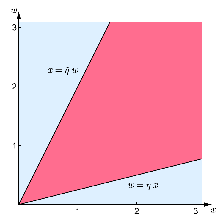
Figure 1: Illustration of the undeformed Amplituhedron geometry (first quadrant, in light blue), for $\eta=\tilde{\eta}=0$, and of the deformed geometry (wedge, in red) for $\eta=\frac{1}{4}$, $\tilde{\eta}=\frac{1}{2}$.

The boundary structure of the deformed Amplituhedron happens to be much simpler than of the original space. Thanks to the deformation parameters, all collinear configurations are removed as boundaries. As a consequence, the number of boundaries of the highest codimension (leading singularities) is only two rather than six: only the configurations with $(AB)_{i}=13$ and $(AB)_{i}=24$ remain, while all other soft-collinear configurations $(AB)_{i}=k\,k{+}1$ are not present. At one-loop, the undeformed Amplituhedron is a positive Grassmannian $G_{+}(2,4)$ with a number of boundaries of various co-dimensions, $(4,10,12,6)$, and Euler characteristic $\chi=+1$. For example, the codimension-two boundaries correspond to four double cuts $\langle AB12\rangle{=}\langle AB23\rangle{=}0$ (and cyclic), each having two solutions – either $AB$ passing $Z_{2}$ or being in the plane $(Z_{1}Z_{2}Z_{3})$, and two double cuts $\langle AB12\rangle{=}\langle AB34\rangle{=}0$ and $\langle AB23\rangle{=}\langle AB14\rangle{=}0$, totaling 10 codimension-two boundaries. In the deformed case any double cut, $\langle AB\hat{X}_{i}\rangle=\langle AB\hat{X}_{j}\rangle=0$, has only one solution, hence we have only six codimension-two boundaries. The number of boundaries of various co-dimensions is now $(4,6,4,2)$, which demonstrates the simplicity of the geometry. The Euler characteristic is again $\chi=+1$.

III Two-loop integrand

At two-loops, the geometric space is more involved and the direct triangulation, though possible, is more difficult. Therefore here we determine the form by making the following ansatz,

$$\Omega^{(2)}=\frac{d\mu_{AB}d\mu_{CD}\cdot{\cal N}(AB,CD,Z_{i},\rho,\tilde{\rho},\eta,\tilde{\eta})}{\bigg{\{}\begin{array}[]{c}\langle AB\hat{X}_{1}\rangle\langle AB\hat{X}_{2}\rangle\langle AB\hat{X}_{3}\rangle\langle AB\hat{X}_{4}\rangle\langle ABCD\rangle\\ \langle CD\hat{X}_{1}\rangle\langle CD\hat{X}_{2}\rangle\langle CD\hat{X}_{3}\rangle\langle CD\hat{X}_{4}\rangle\end{array}\bigg{\}}}\,,$$ (9)

which is based on the known denominator structure and impose consistency conditions on the numerator. One of these conditions is the absence of “non-planar” cuts, which violate the $\langle ABCD\rangle>0$ condition. For example, we can cut following propagators,

$$\langle AB\hat{X}_{1}\rangle=\langle AB\hat{X}_{2}\rangle=\langle CD\hat{X}_{1}\rangle=\langle CD\hat{X}_{2}\rangle=0\,,$$ (10)

which fixes $y_{1}=\rho z_{1}$, $y_{2}=\rho z_{2}$, $w_{1}=\eta x_{1}$, $w_{2}=\eta x_{2}$. Then evaluating $\langle ABCD\rangle$ in this parametrization gives

$$\langle ABCD\rangle=-\rho(z_{1}-z_{2})^{2}-\eta(x_{1}-x_{2})^{2}\,.$$ (11)

This expression is manifestly negative, which is in tension with the $\langle ABCD\rangle>0$ condition. Hence this cut is unphysical and the numerator must vanish when evaluated on it. Imposing all such conditions the ansatz reduces to the sum of deformed double-box integrals (in analogy with the non-deformed case),

$$\Omega^{(a)}_{\rm db} =-\frac{d\mu_{AB}d\mu_{CD}\cdot\langle\hat{X}_{1}\hat{X}_{3}\rangle^{2}\langle\hat{X}_{2}\hat{X}_{4}\rangle}{\bigg{\{}\begin{array}[]{c}\langle AB\hat{X}_{1}\rangle\langle AB\hat{X}_{2}\rangle\langle AB\hat{X}_{3}\rangle\langle ABCD\rangle\\ \langle CD\hat{X}_{3}\rangle\langle CD\hat{X}_{4}\rangle\langle CD\hat{X}_{1}\rangle\end{array}\bigg{\}}},$$ (14)

$$\Omega^{(b)}_{\rm db} =-\frac{d\mu_{AB}d\mu_{CD}\cdot\langle\hat{X}_{1}\hat{X}_{3}\rangle\langle\hat{X}_{2}\hat{X}_{4}\rangle^{2}}{\bigg{\{}\begin{array}[]{c}\langle AB\hat{X}_{2}\rangle\langle AB\hat{X}_{3}\rangle\langle AB\hat{X}_{4}\rangle\langle ABCD\rangle\\ \langle CD\hat{X}_{4}\rangle\langle CD\hat{X}_{1}\rangle\langle CD\hat{X}_{2}\rangle\end{array}\bigg{\}}}.$$ (17)

and $\Omega^{(2)}$ is a symmetrized sum in $AB\leftrightarrow CD$,

$$\Omega^{(2)}=n^{(2a)}\Omega^{(a)}_{\rm db}+n^{(2b)}\Omega^{(b)}_{\rm db}+(AB\leftrightarrow CD)$$ (18)

Unlike in the massless case there is no cancellation of spurious cuts between $\Omega^{(a)}_{\rm db}$ and $\Omega^{(b)}_{\rm db}$, and their coefficients $n^{(2a)}$ and $n^{(2b)}$ are unrelated.

IV Amplitudes from Deformed Amplituhedron

The Amplituhedron defines the planar $L$-loop integrand $\Omega^{(L)}$ at all orders in perturbation theory. More concretely, working with the amplitude, normalized by its tree-level contribution, we have

$$M=1+g^{2}M^{(1)}+g^{4}M^{(2)}+{\cal{O}}(g^{6})\,,$$ (19)

with $g^{2}=g_{\rm YM}^{2}N_{c}/(16\pi^{2})$, and

$$M^{(L)}=\int\Omega^{(L)}\,.$$ (20)

The $L$-loop integrand $\Omega^{(L)}$ is the form with logarithmic singularities on the boundaries of the deformed Amplituhedron space.

The one-loop form associated to the deformed Amplituhedron is found to be

$$\Omega^{(1)}=-n^{(1)}\frac{d\mu_{AB}\langle\hat{X}_{1}\hat{X}_{3}\rangle\langle\hat{X}_{2}\hat{X}_{4}\rangle}{\langle AB\hat{X}_{1}\rangle\langle AB\hat{X}_{2}\rangle\langle AB\hat{X}_{3}\rangle\langle AB\hat{X}_{4}\rangle}\,,$$ (21)

where $d\mu_{AB}=\langle ABd^{2}A\rangle\langle ABd^{2}B\rangle$ is measure in momentum twistor space, normalized such that Arkani-Hamed et al. (2012)

$$\int\frac{d\mu_{AB}}{\langle ABQ\rangle^{4}}=\frac{1}{\Gamma(4)}\frac{1}{\left(\frac{1}{2}\langle QQ\rangle\right)^{2}}\,.$$ (22)

The normalization $n^{(1)}$ is not determined by the Amplituhedron, and it is related to the value of the leading singularity – in the undeformed case the latter is equal to 1. Note that in general, $n^{(1)}$ is a function of the deformation parameters $\rho,\tilde{\rho},\eta,\tilde{\eta}$.

Thanks to dual conformal symmetry, the integrated amplitude $M$ depends on two invariants only, which are

$$u=\frac{\langle\hat{X}_{1}\hat{X}_{3}\rangle^{2}}{\hat{X}_{1}^{2}\hat{X}_{3}^{2}}\,,\qquad v=\frac{\langle\hat{X}_{2}\hat{X}_{4}\rangle^{2}}{\hat{X}_{2}^{2}\hat{X}_{4}^{2}}\,,$$ (23)

which in terms of deformation parameters are given by $(1+\rho\tilde{\rho})^{2}/(4\rho\tilde{\rho})$ and $(1+\eta\tilde{\eta})^{2}/(4\eta\tilde{\eta})$, respectively.

V Comparison to Coulomb-branch amplitudes

Figure 2: One-loop box integral in the deformed Amplituhedron kinematics. The on-shell conditions read $p_{i}^{2}=m_{i}^{2}+m_{i+1}^{2}$, with $m_{5}\equiv m_{1}$.

Interestingly, our deformation leads to massive particles, without the need of introducing an infinity twistor. Translating the kinematics of the deformed Amplituhedron from momentum twistor space to ordinary momentum space, we find that the amplitude corresponds to scattering of particles, as shown in Figure 2. The masses are simple functions of the deformation parameters, and vanish when the latter are sent to zero. The dual conformal invariants are related to the kinematics as follows,

$$u=\frac{(-s+m_{1}^{2}+m_{3}^{2})^{2}}{4m_{1}^{2}m_{3}^{2}}\,,\quad v=\frac{(-t+m_{2}^{2}+m_{4}^{2})^{2}}{4m_{2}^{2}m_{4}^{2}}\,,$$ (24)

where $s=(p_{1}+p_{2})^{2}$, $t=(p_{2}+p_{3})^{2}$. Thanks to the masses, the amplitude is infrared finite. This finiteness property is built into our geometric setup: it can be seen as a consequence of the absence of collinear and soft-collinear regions in the boundary structure of the deformed Amplituhedron.

Our setup is reminiscent of the AdS-inspired Coulomb branch amplitudes Alday et al. (2010); Correa et al. (2012a), where one considers a Higgs mechanism $U(4+N)\to U(4)\times U(N)$. This is done by choosing vacuum expectation values in the $U(4)$ part as follows,

$$\langle{\Phi}\rangle=\frac{1}{g}{\rm diag}(m_{1}\vec{n}_{1},m_{2}\vec{n}_{2},m_{3}\vec{n}_{3},m_{4}\vec{n}_{4})\,,$$ (25)

where $\vec{n}_{i}$ are $SO(6)$ vectors. In Alday et al. (2010), all $\vec{n}_{i}$ were chosen to be equal, which lead to a certain mass configuration. Instead, we find that we can match the mass configuration above by choosing $\vec{n}_{1}=-\vec{n}_{3}$, $\vec{n}_{2}=-\vec{n}_{4}$, with $\vec{n}_{1}\cdot\vec{n}_{2}=0$. We conjecture that the deformed Amplituhedron describes these Coulomb branch amplitudes. If this conjecture is true, then we can use unitarity of the Coulomb branch amplitudes to determine the relative coefficients of the positive geometries. Indeed, performing a one-loop computation as in Appendix B of Alday et al. (2010), we find that $n^{(1)}=1$, and likewise one may fix $n^{(2a)}=n^{(2b)}=1$ from generalized unitarity.

VI Integrated one- and two-loop amplitudes

For carrying out the integration, we find it convenient to parametrize the kinematics as follows,

$$\rho=\tilde{\rho}=-x\,,\quad\eta=\tilde{\eta}=-y\,.$$ (26)

with $0<x<1,0<y<1$. This corresponds to a subset of the Euclidean kinematic region, where the answer is real-valued . Note that this is different from the Amplituhedron region. The cross-ratios of eq. (23) then take the form

$$u=\frac{1}{4}\left(x+\frac{1}{x}\right)^{2}\,,\qquad v=\frac{1}{4}\left(y+\frac{1}{y}\right)^{2}\,.$$ (27)

Starting from eqs. (20) and (21), one may obtain a parameter integral representation for $M^{(1)}$ by introducing Feynman parameters, and then using the basic identity (22), with the result

$$M^{(1)}(x,y) =-{\frac{(1-x)(1-y)}{(1+x)(1+y)}}\int_{0}^{\infty}\frac{d^{4}\alpha}{GL(1)}\times$$ (28)

$$\frac{(1-x^{2})\,(1-y^{2})}{[(\alpha_{1}x+\alpha_{3})(\alpha_{1}+\alpha_{3}x)+(\alpha_{2}y+\alpha_{4})(\alpha_{2}+\alpha_{4}y)]^{2}}\,.$$

Carrying out the integration yields a surprisingly simple answer,

$$M^{(1)}(x,y)=-2{\frac{(1-x)(1-y)}{(1+x)(1+y)}}\log(x)\log(y)\,.$$ (29)

At two loops, we have

$$M^{(2)}(x,y)=I_{\rm db}(x,y)+I_{\rm db}(y,x)\,,$$ (30)

where

$$I_{\rm db}(x,y)=\int\Omega^{(a)}_{\rm db}\,,\qquad I_{\rm db}(y,x)=\int\Omega^{(b)}_{\rm db}\,.$$ (31)

Leveraging four-dimensional differential equation techniques Caron-Huot and Henn (2014) we find that, remarkably, the answer for the double box can be written in just a few lines,

$$I_{\rm db}(x,y)= {\frac{(1-x)^{2}(1-y)}{(1+x)^{2}(1+y)}}\Big{[}J_{3}(x^{2})\log(y^{2})$$

$$-Q(y^{2})+\frac{1}{2}Q\left(\frac{y^{2}}{x^{2}}\right)+\frac{1}{2}Q(x^{2}y^{2})\Big{]}\,,$$ (32)

with

$$Q(z) =3\text{Li}_{4}(z)-3\log(z)\text{Li}_{3}(z)+\frac{3}{2}\log^{2}(z)\text{Li}_{2}(z)$$

$$+\frac{1}{2}\log^{3}(z)\log(1-z)+\frac{3\pi^{4}}{10}+\frac{\pi^{2}}{4}\log^{2}\left(z\right)$$

$$+\frac{3}{16}\log^{4}\left(z\right)+\log^{2}\left(z\right){\rm Li}_{2}(1-z)+4\pi^{2}{\rm Li}_{2}\left(-\sqrt{z}\right)$$

$$-\log\left(z\right){\rm Li}_{3}\left(1-\frac{1}{z}\right)-\log\left(z\right){\rm Li}_{3}\left(1-{z}\right)\,,$$ (33)

and

$$\begin{split}J_{3}(z)&=\frac{1}{4}\log^{3}\left(z\right)+\log\left(z\right){\rm Li}_{2}\left(1-{z}\right)\\ &-2{\rm Li}_{3}\left(1-{z}\right)-2{\rm Li}_{3}\left(1-\frac{1}{z}\right)\,.\end{split}$$ (34)

$Q$ and $J_{3}$ are real-valued for positive arguments. As in the famous result for the six-gluon two-loop remainder function in sYM Goncharov et al. (2010), only classical polylogarithms are needed. In contrast, the two-loop four-particle amplitude in the (slightly different) Coulomb-branch setup of Alday et al. (2010) is more complicated Caron-Huot and Henn (2014) .

We also note that the amplitude up to two loops has the following ten-letter symbol alphabet,

$$\begin{split}{\cal A}=&\{x,1\pm x,y,1\pm y,x\pm y,1\pm xy\}\,.\end{split}$$ (35)

It is interesting to study the behavior of $M$ near singular kinematic configurations, i.e. where one or more terms in eq. (35) vanish. We now present exact formulas for the leading behavior in two such limits.

VII Exact results in kinematic limits

High-energy limit. This corresponds to $s,t\to\infty$, or equivalently, $x,y\to 0$, keeping $x/y=t/s$ fixed. This limit where the deformation parameters are taken to zero allows us to connect to the massless, infrared-divergent amplitude. We conjecture that the following exact formula holds in the high-energy limit,

$$\begin{split}\log M\stackrel{{\scriptstyle x,y\to 0}}{{=}}&-\frac{1}{2}\Gamma_{\rm cusp}(g)\log x\log y\\ &+\Gamma_{\rm collinear}(g)\left(\log x+\log y\right)+{C}(g)\,,\end{split}$$ (36)

which is analogous to formulas in dimensional regularization Bern et al. (2005); Drummond et al. (2010) and on the Coulomb branch Alday et al. (2010). Here $\Gamma_{\rm cusp}=4g^{2}-8\zeta_{2}g^{4}+{\cal O}(g^{6})$ is the light-like cusp anomalous dimension, which is famously known from integrability Beisert et al. (2007). Comparing to our perturbative results, we find that (36) holds with the collinear anomalous dimension $\Gamma_{\rm collinear}(g)=-4\zeta_{3}g^{4}+{\cal O}(g^{6})$ and ${C}(g)=-3/10\pi^{4}g^{4}+{\cal O}(g^{6})$. The latter two are both regularization-scheme dependent Henn et al. (2011).

Regge limit $t\to\infty$. This corresponds to $y\to 0$, keeping $x$ fixed. Thanks to dual conformal symmetry, this may be equivalently viewed as the small mass $m_{1}\to 0$ limit. Therefore we expect this limit to be governed by eikonal physics Henn et al. (2010), and in particular by the anomalous dimension of a cusped Wilson loop, which to two loops is given by Drukker and Forini (2011)

$$\Gamma_{\rm cusp}(\phi,\theta;g)= g^{2}\xi(-2\log x)+$$ (37)

$$+g^{4}\Bigg{\{}\xi\frac{4}{3}\log x\left(\pi^{2}+\log^{2}x\right)+\xi^{2}\Bigg{[}4\text{Li}_{3}\left(x^{2}\right)$$

$$-4\text{Li}_{2}\left(x^{2}\right)\log(x)-\frac{4}{3}\log^{3}(x)-\frac{2}{3}\pi^{2}\log(x)-4\zeta_{3}\Bigg{]}\Bigg{\}}\,.$$

Here the Euclidean cusp angle $\phi$ is related to $x$ via $x=e^{i\phi}$, and the second parameter $\theta$ parametrizes the Wilson loop’s coupling to scalars, via the combination

$$\xi=\frac{\cos\theta-\cos\phi}{i\sin\phi}=\frac{1+x^{2}-2x\cos\theta}{1-x^{2}}\,.$$ (38)

The choice of SO(6) vectors we made below eq. (25) suggests that here $\theta=0$, which implies $\xi=(1-x)/(1+x)$. Indeed, we find that the leading terms in the Regge limit are given by

$$M(x=e^{i\phi},y)\stackrel{{\scriptstyle y\to 0}}{{=}} r(\phi,0;g)\,y^{\Gamma_{{\rm cusp}}(\phi;0;g)}+{\cal O}({y^{0}})\,,$$ (39)

where $r(\phi,0;g)$ being the finite part in the Regge limit. It is interesting to note that by making a more general choice of $SO(6)$ vectors in eq. (25), such that $\vec{n}_{1}\cdot\vec{n}_{3}=-\cos\theta$, we can match the full $\xi$ dependence.

VIII Summary and Outlook

We generalized the four-particle Amplituhedron geometry of planar sYM such that the amplitude $M(x,y)$ is infrared finite and depends on two dual conformal parameters $x,y$. The finiteness is due to massive propagators. The mass configuration is different from the Coulomb branch setup of Alday et al. (2010), but we found that a slightly different pattern of vacuum expectation values matches our geometric setup. It remains to be proven that the deformed Amplituhedron not only matches the kinematics, but gives exactly those Coulomb branch amplitudes.

In the original Amplituhedron, fixing the integrand involved the assumption of normalizing the canonical forms to have unit (constant) leading singularities on certain boundaries. Instead, the Coulomb branch amplitudes in general have kinematic-dependent leading singularities. This means that a generalization is needed of how we think about canonical forms. In this Letter, we fixed those normalizations by comparing against generalized cuts of Coulomb branch amplitudes. One may ask – are there other ways of fixing the answer that do not refer to field theory at all?

Given the two-loop integrand obtained in this way, we computed the analytic result for $M(x,y)$ up to two loops, and conjectured exact formulas both in the high-energy as well as the Regge limit. Given the relatively simple symbol alphabet that we uncovered, it may be possible to bootstrap higher-loop results, given sufficient physical input from limiting configurations and analytic properties (for a review see Caron-Huot et al. (2020)).

We expect that the new setup will lead to substantial progress in making the connection between geometry and the integrated functions, benefiting from recent work in mathematics Even-Zohar et al. (2021). This could lead to a geometry-based differential equations method, with broader applications.

Our novel starting point also gives completely new ways of studying physical limits, and to potentially obtain exact results. Thanks to the simpler geometric configurations in the limit, obtaining the canonical form and integrating it should be easier. One particularly interesting example is the $\phi\to 0$ limit of the angle-dependent cusp anomalous dimension, whose first term $\Gamma_{\rm cusp}(\phi,\theta=0;g)=-\phi^{2}B(g)+{\cal O}(\phi^{4})$ is the exactly-known Bremsstrahlung function Correa et al. (2012b).

References

- Alday and Maldacena (2007) L. F. Alday and J. M. Maldacena, JHEP 06, 064 (2007), arXiv:0705.0303 [hep-th] .
- Arkani-Hamed and Trnka (2014a) N. Arkani-Hamed and J. Trnka, JHEP 10, 030 (2014a), arXiv:1312.2007 [hep-th] .
- Arkani-Hamed et al. (2018) N. Arkani-Hamed, H. Thomas, and J. Trnka, JHEP 01, 016 (2018), arXiv:1704.05069 [hep-th] .
- Karp and Williams (2019) S. N. Karp and L. K. Williams, Int. Math. Res. Not. 5, 1401 (2019), arXiv:1608.08288 [math.CO] .
- Karp et al. (2020) S. N. Karp, L. K. Williams, and Y. X. Zhang, Ann. Inst. H. Poincare D Comb. Phys. Interact. 7, 303 (2020), arXiv:1708.09525 [math.CO] .
- Lukowski et al. (2020) T. Lukowski, M. Parisi, and L. K. Williams, (2020), arXiv:2002.06164 [math.CO] .
- Parisi et al. (2021) M. Parisi, M. Sherman-Bennett, and L. Williams, (2021), arXiv:2104.08254 [math.CO] .
- Even-Zohar et al. (2021) C. Even-Zohar, T. Lakrec, and R. J. Tessler, (2021), arXiv:2112.02703 [math-ph] .
- Blot and Li (2022) X. Blot and J.-R. Li, (2022), arXiv:2206.03435 [math.CO] .
- Arkani-Hamed and Trnka (2014b) N. Arkani-Hamed and J. Trnka, JHEP 12, 182 (2014b), arXiv:1312.7878 [hep-th] .
- Franco et al. (2015) S. Franco, D. Galloni, A. Mariotti, and J. Trnka, JHEP 03, 128 (2015), arXiv:1408.3410 [hep-th] .
- Arkani-Hamed et al. (2015) N. Arkani-Hamed, A. Hodges, and J. Trnka, JHEP 08, 030 (2015), arXiv:1412.8478 [hep-th] .
- Arkani-Hamed et al. (2019) N. Arkani-Hamed, C. Langer, A. Yelleshpur Srikant, and J. Trnka, Phys. Rev. Lett. 122, 051601 (2019), arXiv:1810.08208 [hep-th] .
- Herrmann et al. (2021) E. Herrmann, C. Langer, J. Trnka, and M. Zheng, JHEP 01, 035 (2021), arXiv:2009.05607 [hep-th] .
- Dian et al. (2022) G. Dian, P. Heslop, and A. Stewart, (2022), arXiv:2207.12464 [hep-th] .
- Herrmann and Trnka (2022) E. Herrmann and J. Trnka, J. Phys. A 55, 443008 (2022), arXiv:2203.13018 [hep-th] .
- Arkani-Hamed et al. (2022) N. Arkani-Hamed, J. Henn, and J. Trnka, JHEP 03, 108 (2022), arXiv:2112.06956 [hep-th] .
- Damgaard et al. (2019) D. Damgaard, L. Ferro, T. Lukowski, and M. Parisi, JHEP 08, 042 (2019), arXiv:1905.04216 [hep-th] .
- Ferro and Lukowski (2023) L. Ferro and T. Lukowski, JHEP 05, 183 (2023), arXiv:2210.01127 [hep-th] .
- He et al. (2023) S. He, Y.-t. Huang, and C.-K. Kuo, (2023), arXiv:2306.00951 [hep-th] .
- Britto et al. (2005) R. Britto, F. Cachazo, B. Feng, and E. Witten, Phys. Rev. Lett. 94, 181602 (2005), arXiv:hep-th/0501052 .
- Arkani-Hamed et al. (2012) N. Arkani-Hamed, J. L. Bourjaily, F. Cachazo, and J. Trnka, JHEP 06, 125 (2012), arXiv:1012.6032 [hep-th] .
- Alday et al. (2010) L. F. Alday, J. M. Henn, J. Plefka, and T. Schuster, JHEP 01, 077 (2010), arXiv:0908.0684 [hep-th] .
- Correa et al. (2012a) D. Correa, J. Henn, J. Maldacena, and A. Sever, JHEP 05, 098 (2012a), arXiv:1203.1019 [hep-th] .
- Note (1) We note that it is also possible to switch on further angles, such that and .
- Note (2) Note that although the cross-ratios are seemingly independent e.g. under , this transformation requires analytic continuation. See e.g. Duplancic, Nizic, Eur.Phys.J.C 24 (2002) for a related discussion.
- Caron-Huot and Henn (2014) S. Caron-Huot and J. M. Henn, JHEP 06, 114 (2014), arXiv:1404.2922 [hep-th] .
- Goncharov et al. (2010) A. B. Goncharov, M. Spradlin, C. Vergu, and A. Volovich, Phys. Rev. Lett. 105, 151605 (2010), arXiv:1006.5703 [hep-th] .
- Bern et al. (2005) Z. Bern, L. J. Dixon, and V. A. Smirnov, Phys. Rev. D 72, 085001 (2005), arXiv:hep-th/0505205 .
- Drummond et al. (2010) J. M. Drummond, J. Henn, G. P. Korchemsky, and E. Sokatchev, Nucl. Phys. B 826, 337 (2010), arXiv:0712.1223 [hep-th] .
- Beisert et al. (2007) N. Beisert, B. Eden, and M. Staudacher, J. Stat. Mech. 0701, P01021 (2007), arXiv:hep-th/0610251 .
- Henn et al. (2011) J. M. Henn, S. Moch, and S. G. Naculich, JHEP 12, 024 (2011), arXiv:1109.5057 [hep-th] .
- Henn et al. (2010) J. M. Henn, S. G. Naculich, H. J. Schnitzer, and M. Spradlin, JHEP 04, 038 (2010), arXiv:1001.1358 [hep-th] .
- Drukker and Forini (2011) N. Drukker and V. Forini, JHEP 06, 131 (2011), arXiv:1105.5144 [hep-th] .
- Caron-Huot et al. (2020) S. Caron-Huot, L. J. Dixon, J. M. Drummond, F. Dulat, J. Foster, O. Gürdoğan, M. von Hippel, A. J. McLeod, and G. Papathanasiou, PoS CORFU2019, 003 (2020), arXiv:2005.06735 [hep-th] .
- Correa et al. (2012b) D. Correa, J. Henn, J. Maldacena, and A. Sever, JHEP 06, 048 (2012b), arXiv:1202.4455 [hep-th] .