Hamiltonian Forging of a Thermofield Double

Abstract

We address the variational preparation of Gibbs states as the ground state of a suitably engineered Hamiltonian acting on the doubled Hilbert space. The construction is exact for quadratic fermionic Hamiltonians and gives excellent approximations up to fairly high quartic deformations. We provide a variational circuit whose optimization returns the unitary diagonalizing operator, thus giving access to the whole spectrum. The problem naturally implements the entanglement forging ansatz, allowing the computation of Thermofield Doubles with a higher number of qubits than in competing frameworks.

State preparation is of central importance in quantum computation, and it cannot be disentangled from the algorithmic prescription of a quantum task. When dealing with circuits that simulate quantum thermal processes, both at and out of equilibrium, the initial state that one needs to prepare is, typically, the Gibbs state, whose purification is the Thermofield Double (TFD) state. The preparation of the TFD state is potentially as hard a task as that of finding the ground state of a generic Hamiltonian [1, 2]. Such initial state has emerged as a valuable tool to study thermal behavior of quantum systems [3, 4, 5, 6]. It is also relevant for the simulation of gravity duals to black holes and wormholes [7, 8].

Variational quantum algorithms have become a practical method to prepare quantum states across different domains in quantum simulation. In relation to the present context, a number of works have proposed to generate the TFD state by minimizing the Helmholtz free energy [9, 10, 11]. Here different works differ mainly in the variational ansatz. All of them, however, face the difficulty of having to compute the von Neumann entropy on the fly, and some ideas have been proposed to accomplish this task [12, 13, 14].

In this letter, we also address the preparation of the TFD state by variational quantum computation but, instead of the free energy, we will minimize the energy of an ad hoc designed Hamiltonian. The idea is inspired by the similar mechanism proposed and studied in [15, 16, 17] although we will be working in the opposite weakly coupled limit that perturbs around the free fermion case.

Variational optimizations are hindered by the trainability of the variational ansatz selected. We propose one that is naturally adapted to the structure of the TFD. It is amenable to a protocol known as Entanglement Forging (EF)[18], a rather simplified version of the circuit cutting/knitting technique which allows addressing the preparation of the TFD for $2N$ qubits while running quantum circuits of width $N$.

As an extra benefit, by design, the minimization of the variational circuit yields precisely the unitary matrix that diagonalizes the Hamiltonian of the theory. This feature, which can also be found in [14], provides access to the whole spectrum and provides an alternative to standard deflationary approaches [19], which are based on iteratively adding penalty terms associated to rank-1 projectors.

This letter is structured as follows. First we introduce the main idea and exemplify its performance on a generic fermionic model. In the next section we present the variational forging ansatz used to actually prepare the TFD state on a quantum computer. Finally we show the results and conclude with comments.

I TFD States as Ground States

Given a Hamiltonian $H$, the associated Gibbs state, $\rho=e^{-\beta H}/Z$, characterizes equilibrium in the canonical ensemble at temperature $T=1/\beta$. The purification of this state, known as the Thermofield Double, requires the duplication of the number of degrees of freedom of the system [20]. We will focus on purifications of the following form

$$|\hbox{TFD}(\beta)\rangle=\sum_{n}e^{-\beta E_{n}}|E_{n}\rangle\otimes|E^{*}_{n}\rangle$$ (1)

where $|E^{*}_{n}\rangle$ stands for the complex conjugate basis. The promise is that there exists a certain Hamiltonian, $H_{tot}(\beta)$, in the enlarged Hilbert space, whose ground state $|\hbox{GS}(\beta)\rangle$ is, with high overlap, the sought-after TFD

$$|\langle\hbox{GS}(\beta)|\hbox{TFD}(\beta)\rangle|\approx 1\,.$$

Concrete expressions for $H_{tot}$ have been proposed in the literature, and they range from exact but impracticable [16], to simple but approximate [16, 15, 17]. In the second case, the proposed Hamiltonians have the generic structure $H_{tot}(\beta)=H_{L}+H_{R}+H_{LR}(\beta)$, where $H_{L}=H\otimes I$, $H_{R}=I\otimes H^{*}$ and, therefore, it only remains to say what is $H_{LR}$. A very general prescription is that $H_{LR}$ is a Hamiltonian whose ground state exhibits maximal entanglement, hence equal to the infinite temperature $|\hbox{TFD}(\beta\to 0)\rangle$. At the opposite end, i.e. at low temperature, $H_{LR}(\beta\to\infty)$ should vanish, making the overlap maximal with the ground state of $H_{L}+H_{R}$, hence equal to the zero temperature $|\hbox{TFD}(\beta\to\infty)\rangle=|E_{0}\rangle\otimes|E^{*}_{0}\rangle$.

Outside these limits, $H_{LR}(\beta)$ should be carefully readjusted so as to keep the overlap $|\langle\hbox{GS}(\beta)|\hbox{TFD}(\beta)\rangle|$ as close to 1 as possible. In the cited references, no controlled scheme is offered by means of which one can obtain an estimation of the departure from maximal fidelity. In the next section, we seek for such a protocol by starting from an exact answer valid for the case of free fermions. The introduction of an interaction degrades this maximal fidelity in a continuous way. We provide a set of rules to still find an excellent answer.

I.1 Fermionic models

We start by looking at fermionic systems and assume to work in a quasi-particle basis in which the free (quadratic) piece has been brought to its diagonal form. Hence, the general case can be written as follows

$$H = \sum_{i}\omega_{i}a^{\dagger}_{i}a_{i}+\sum_{ijkl}U_{ijkl}a_{i}^{\dagger}a_{j}^{\dagger}a_{k}a_{l}+...$$ (2)

$$= H_{2}+H_{4}+...$$

with $\omega_{i}\in{\mathbb{R}}$ nonzero real numbers. To start with, consider the free-fermion limit $H=H_{2}$. To find the TFD as a ground state, we double the Hilbert space and enlarge accordingly the set of operators $a_{i}\to a_{i}^{L}=a_{i}\otimes I,a_{i}^{R}=I\otimes a_{i}$. In this free-fermion limit, an exact solution for

$$H_{tot}(\beta)=H_{L}+H_{R}+H_{LR}$$ (3)

exists, and is given by

$$H_{L} = \sum_{i}\omega_{i}a^{L\dagger}_{i}a^{L}_{i}\leavevmode\nobreak\ \leavevmode\nobreak\ ,\leavevmode\nobreak\ \leavevmode\nobreak\ H_{R}=\sum_{i}\omega_{i}a^{R\dagger}_{i}a^{R}_{i}\leavevmode\nobreak\ \leavevmode\nobreak\ ,$$ (4)

$$H_{LR} = \sum_{i}\mu_{i}(\beta)(a^{L}_{i}a^{R}_{i}-a^{L\dagger}_{i}a^{R\dagger}_{i}),$$

with

$$\mu_{i}(\beta)=\frac{\omega_{i}}{2\sinh\beta\omega_{i}/2}\,.$$ (5)

A proof of this statement can be found in the Supplemental Material. The overlap $|\langle\hbox{GS}(\beta)|\hbox{TFD}(\beta)\rangle|=1$ is maximal, for all values of $\beta$.

A four-fermion interaction like $H_{4}$ in (2) makes the situation depart from the free exact case. The question now is twofold: a) how should we modify the $H_{LR}$ Hamiltonian so as to maintain the overlap as close to one as possible? b) how large can $H_{4}$ be made in order to stay globally within some tolerance, say, $|\langle\hbox{GS}(\beta)|\hbox{TFD}(\beta)\rangle|\geq 0.99$.

For the first question, a minimal answer would be to stick to the same structure as in (3) and (4), and only modify the set of numbers $\omega_{i}\to\tilde{\omega}_{i}=\omega_{i}+\delta\omega_{i}$ which are then plugged into (5) to construct the improved LR interaction. The shifts $\delta\omega_{i}$ should be readable from the structure of the perturbing Hamiltonian $H_{4}$. An educated guess is to extract them from a mean-field calculation.

In regard to the second question, the construction now is no longer exact and we expect the overlap to drop below 1 for intermediate values of $\beta$. The answer needs a case-by-case analysis. We illustrate it with an example in the next sections.

I.2 Numerical test: the Hubbard spinless chain

To get an insight into the answer to the previous questions, a numerical analysis is in order. We will consider a popular benchmark model, the Hubbard 1D chain. Since we are not interested in magnetization phenomena, we will consider a simplified version with spinless fermions on N sites:

$$H=\sum_{i=1}^{N}\epsilon_{0}a^{\dagger}_{i}a_{i}-t\left(\sum_{i=1}^{N}a^{\dagger}_{i}a_{i+1}+h.c\right)+U\sum_{i=1}^{N}a_{i}^{\dagger}a_{i}a_{i+1}^{\dagger}a_{i+1}\,.$$ (6)

Quadratic terms encode the on-site potential and nearest-neighbor interactions. They are weighted by a chemical potential $\epsilon_{0}$ and hopping amplitude $t$, respectively. The quartic terms introduce nearest neighbor repulsion parametrized by a constant $U$. To bring this Hamiltonian into the form (2), the change of basis needed is just a simple Fourier transform (assuming periodic boundary conditions), after which

$$H=\sum_{k}\omega_{k}a^{\dagger}_{k}a_{k}+\frac{U}{N}\sum_{k,p,q}e^{-i\frac{2\pi}{N}q}\;a^{\dagger}_{k+q}a_{k}a^{\dagger}_{p-q}a_{p}\,,$$ (7)

where $\omega_{k}=\epsilon_{0}-2t\cos(2\pi k/N)$, with $k=0,..,N-1$. The interaction term proportional to $U$ is non-local in momentum. It gives rise now to scattering events between two incoming electrons with momentum $k$ and $p$ that exchange momentum $q$. As previously discussed, the model with only $H_{2}$ is exactly solvable. Adding $H_{4}$ makes the overlap $|\langle\hbox{GS}(\beta)|\hbox{TFD}(\beta)\rangle|$ decrease if this quartic interaction introduces a significant contribution that competes with the diagonal $H_{2}$. In this example, such contributions arise from scattering terms with net momentum exchange zero, i.e., $q=0$ and $k+q=p$. The non-interacting energies $\omega_{k}$ are not the best candidates to estimate $H_{LR}$ and generate a TFD with optimal overlap with the GS (see Supplementary Material).

As advertised previously, an educated guess to improve the efficacy of the interaction Hamiltonian $H_{LR}$ involves shifting the non-interacting $\omega_{k}\to\tilde{\omega}_{k}=\omega_{k}+\delta\omega_{k}$ appropriately. A natural candidate for $\delta\omega_{k}$ comes from the diagonal mean-field contribution of $H_{4}$ [23, 24], for which $\delta\omega_{k}=2U\rho-2U\alpha\cos{(2\pi k/N)}$. Here, $\rho=\frac{1}{N}\sum_{k^{\prime}}\langle a_{k^{\prime}}^{\dagger}a_{k^{\prime}}\rangle$ is the mean-field value of the density and $\alpha=\frac{1}{N}\sum_{k^{\prime}}\cos{(2\pi k^{\prime}/N)}\langle a_{k^{\prime}}^{\dagger}a_{k^{\prime}}\rangle$ is a contribution that depends on the occupancy level configuration. With this, we find excellent overlaps in the final ground state with the exact TFD. In figure 1, we plot the value of the overlap $|\langle\hbox{GS}(\beta)|\hbox{TFD}(\beta)\rangle|$ for different values of the coupling strength ratio, $U/t$, for a Hubbard ring of $N=6$ sites. In all the temperature range, the overlap remains $\sim 1$.

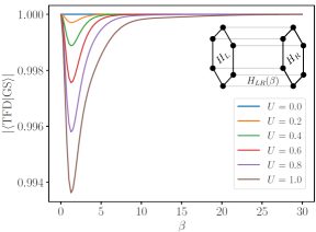
Figure 1: $\left|\langle\hbox{TFD}(\beta)|GS(\beta)\rangle\right|$ for the Hubbard model in frequency space ($t=1$, $\epsilon_{0}=0$, $2N=12$) for different values of $U$. For every $U$, mean-field energies $\tilde{\omega}_{k}(\epsilon_{0},t,U)$ were estimated numerically by minimizing the free energy. The figure shows how the prescription for $H_{LR}$ leads to TFDs with high overlaps with the GS of $H_{tot}$.

In summary, we have provided a scheme in which, with controllable accuracy, the problem of finding the TFD state of a certain Hamiltonian $H$ can be traded for an energy minimization problem in an auxiliary LR coupled system.

II Forging a Thermofield Double

The Entanglement Forging protocol [18] is specifically designed to deal with the variational evaluation of the ground state energy in naturally bi-partitioned problems such as the TFD. Define, on the $2n$-qubit Hilbert space ${\cal H}={\cal H}_{L}\otimes{\cal H}_{R}$, a general variational state written in the Schmidt form, $|\Psi\rangle=\left(U(\theta)\otimes V(\phi)\right)\sum_{i}\lambda_{i}|b_{i}\rangle\otimes|b_{i}\rangle$, where $|b_{i}\rangle$ stand for the elements of the computational basis and $\lambda$, $\theta$ and $\phi$ are sets of variational parameters. Writing $|\Psi\rangle$ in this form allows to compute any two-side cost function $\langle\Psi|O_{L}\otimes O_{R}|\Psi\rangle$ as a linear combination of one-side expectation values. Nevertheless, the number of variational parameters is very large, already $2^{n}$ just to account for the Schmidt coefficients $\lambda_{i}$.

The bipartite nature of the TFD and its specific form, allows to use a Schmidt ansatz in order to minimize (3). If after an optimization the optimized ansatz $|\Psi_{opt}\rangle$ is equal to the TFD, the Schmidt coefficients must encode the Boltzmann distribution $\lambda_{i}\to\lambda^{opt}_{i}=e^{-\beta E_{i}/2}/Z$. Moreover, $U(\theta_{opt})$ has to be exactly the matrix that rotates the computational basis into the energy eigenbasis $|E_{i}\rangle=U(\theta_{opt})|b_{i}\rangle$, such that $H|E_{i}\rangle=E_{i}|E_{i}\rangle$. Let us, therefore, put forward the following TFD-inspired variational ansatz

$$|\Psi(\theta)\rangle=\sum_{i}\frac{e^{-\beta\tilde{E}_{i}(\theta)/2}}{Z(\beta,\theta)}|f_{i}(\theta)\rangle\otimes|f^{*}_{i}(\theta)\rangle$$ (8)

with $|f_{i}(\theta)\rangle=U(\theta)|b_{i}\rangle,|f^{*}_{i}(\theta)\rangle=U^{*}(\theta)|b_{i}\rangle$, the energy estimators $\tilde{E}_{i}(\theta)=\langle f_{i}(\theta)|H|f_{i}(\theta)\rangle$, and the normalization factor $Z(\beta,\theta)=\sum_{k}e^{-\beta\tilde{E}_{k}(\theta)}$. Notice the reduction in the number of parameters that replaces the Schmidt coefficients $\lambda_{i}$ in favor of $e^{-\beta\tilde{E}_{i}(\theta)}/Z(\theta)$. The evaluation of the expectation value of any operator $O_{L}\otimes O_{R}$ becomes a weighted sum involving only $n$-qubit matrix elements

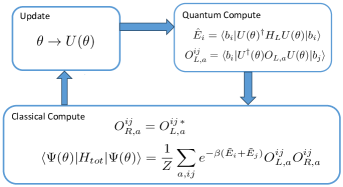
Figure 2: For a Hamiltonian of the form $H_{tot}=H_{L}+H_{R}+H_{LR}=\sum_{a}O_{L,a}\otimes O_{R,a}$ only one sided expectation values need to be evaluated quantumly. The classical part composes and minimizes the global energy cost function $\langle H_{tot}\rangle$

$$\begin{split}\langle\Psi(\theta)|O_{L}\otimes O_{R}&|\Psi(\theta)\rangle_{\beta}=\sum_{i,j}\frac{e^{-\beta(\tilde{E}_{i}(\theta)+\tilde{E}_{j}(\theta))/2}}{Z(\beta,\theta)}\\ &\times\langle f_{i}(\theta)|O_{L}|f_{j}(\theta)\rangle\langle f^{*}_{i}(\phi)|O_{R}|f^{*}_{j}(\phi)\rangle.\end{split}$$ (9)

Given that the cost function is $\langle\Psi(\theta)|H_{tot}|\Psi(\theta)\rangle_{\beta}$ with $H_{tot}=\sum_{a}O_{L,a}\otimes O_{R,a}$, it is clear that, at each round, everything is set in place and the workflow is consistent (see Figure 2). Notice that $\beta$ is not a variational parameter, as it is fixed by $H_{tot}(\beta)$. Finally, the exponentially decaying nature of the Boltzmann coefficients $\lambda_{i}$ allows to truncate the sum in the low-temperature regime $\beta\gg 1$.

Once the minimization is completed, one gets the circuit $U(\theta_{opt})$ that diagonalizes $H$ and its energies $E_{i}$. Importantly, outside the case of free fermions, it is not guaranteed that the full Hamiltonian $H_{tot}$ is perfectly minimized. The reason is that $|\hbox{GS}(\mu)\rangle$ may not be reached as the minimization occurs within the ansatz (8) that only spans TFD-like states. However, it is natural to expect that the optimization will attract the variational state $|\Psi(\theta)\rangle$ to the closest TFD-like state to $|\hbox{GS}\rangle$. Provided that $|\langle\hbox{GS}(\beta)|\hbox{TFD}(\beta)\rangle|\approx 1$, then, $|\langle\Psi(\theta_{opt},\beta)|\hbox{TFD}(\beta)\rangle|\approx 1$. In the remaining part of this letter, we will provide numerical evidence supporting this expectation.

It it is worth noting that this protocol does not prepare the $|\hbox{TFD}\rangle$ as a state but only allows to compute expectation values in it. This is, in principle, enough to compute thermal expectation values. It is possible to recover the $|\hbox{TFD}\rangle$ but it requires to implement the circuit $U_{\lambda}|0\rangle=\sum_{i}\lambda^{opt}_{i}|b_{i}\rangle$. This is a probability loading problem that can be addressed either exactly or variationally following standard techniques [25, 26].

III Simulations and Results

Selecting an adequate variational ansatz for the circuit that generates $U(\theta)$ is necessary in order to forge the TFD as the ground state of $H_{tot}$ [18]. As any other variational algorithm, it can suffer from trainability issues such as local minima or barren plateaus. Moreover, it also has to be expressive enough for the ansatz to approximate as a unitary change of basis onto the eigenstate basis.

With these caveats in mind, we opt for a Hamiltonian Variational Ansatz (HVA) [27, 28] from which we can generate the vectors $|f_{i}({\theta})\rangle=U(\theta)|b_{i}\rangle=\prod_{l}^{\mathcal{L}}\left(\prod_{s}e^{-i\theta_{s,l}h_{s}}\right)|b_{i}\rangle$, directly from the elements of the computational basis, which are the eigenstates of $H_{2}$ in the momentum space. The product is over sets $H_{L}=\sum_{s}h_{s}$, where each set $h_{s}$ is made of commuting operators, while $[h_{s},h_{s}^{\prime}]\neq 0$. By construction, in our case $h_{0}$ is the Jordan-Wigner transformation of $H_{2}$. The index $l$ iterates over the number of layers $\mathcal{L}$.

In Figure 3, the results of the optimizations using scipy’s BFGS optimizer and $\mathcal{L}=1$ for the Hamiltonian given in (7) with parameters $t=1$, $\epsilon_{0}=0$, $U=1$, are evaluated using overlaps and the resulting spectrum as figures of merit. In this model, for the overlaps, we find $\lvert\langle\Psi_{opt}|\hbox{TFD}\rangle\rvert\geq\lvert\langle\hbox{GS}|\hbox{TFD}\rangle\rvert$, which can be interpreted as $|\Psi_{opt}\rangle$ being geometrically located between $|\hbox{GS}\rangle$ and $|\hbox{TFD}\rangle$. Additionally, we compare the exact spectrum $E_{n}$ and the one obtained variationally $\tilde{E}_{n}(\theta_{opt})$ at $\beta=1.26$. We see that they match almost perfectly for $N=4$ and in the low energy tail of $N=6$. Even in this strongly coupled limit ($U=t$), the overlaps after the optimization do not drop below $0.99$, which corroborates the robustness of this protocol.

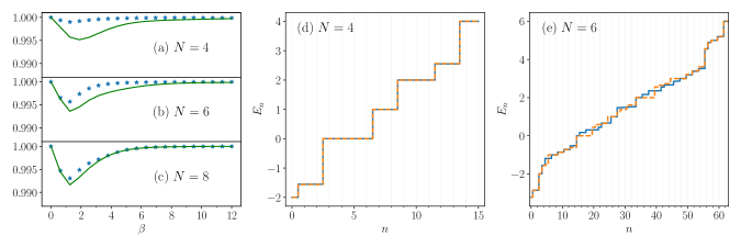
Figure 3: Simulation results for the Hubbard model in frequency space with $t=1$, $\epsilon=0$, $U=1$. (a), (b), (c) Comparison between overlaps, $\lvert\langle\Psi_{opt}|\hbox{TFD}\rangle\rvert$ (blue stars) and $\lvert\langle\hbox{GS}|\hbox{TFD}\rangle\rvert$ (green line) at $N=4,6,8$. The overlaps still remain high in the strongly coupling ($U/t=1$), even after the optimization. (d), (f) Spectrum obtained via exact diagonalization (blue line) and variationally at $\beta=1.26$ (orange line). The variational protocol reproduces the lower energy part of the spectrum almost perfectly. The intermediate part is only matched approximately. This correlates with the fact that the overlap between $|\psi_{opt}\rangle$ and the TFD is not maximal.

IV Conclusions

We have proposed a Hamiltonian variational construction of a TFD. Alongside, it provides access to the full spectrum of eigenvalues and eigenvectors of a given Hamiltonian. The clue is the design of an interaction Hamiltonian whose global ground state is very close to the TFD. The range of applicability is not universal, and restricts to systems that can be mapped onto fermionic Hamiltonians, which are not far from free ones (it would be interesting to leverage this statement with some interaction distance [29]). The variational ansatz is naturally adapted to the use of entanglement forging techniques, thereby allowing to halve the number of qubits of the quantum circuit involved.

V Acknowledgements

We would like to thank Diego Porras, Sebastián V. Romero and Luca Tagliacozzo for interesting discussions.

The work of J.SS. and J.M. was supported by Xunta de Galicia (Centro Singular de Investigacion de Galicia accreditation 2019-2022) and by the Spanish Research State Agency under grant PID2020-114157GB-I00, and by the European Union FEDER. The work of J.S. was supported by MICIN through the European Union NextGenerationEU recovery plan (PRTR-C17.I1), and by the Galician Regional Government through the “Planes Complementarios de I+D+I con las Comunidades Autónomas” in Quantum Communication. D.F. was supported by Axencia Galega de Innovación through the Grant Agreement “Despregamento dunha infraestructura baseada en tecnoloxías cuánticas da información que permita impulsar a I+D+I en Galicia” within the program FEDER Galicia 2014-2020. Simulations in this work were performed using the Finisterrae III Supercomputer, funded by the project CESGA-01 FINISTERRAE III. D.H.M. acknowledges financial support from CEA’s Science Impulse Program.

Supplemental Material:
Hamiltonian Forging of a Thermofield Double

Appendix S1 Quadratic Hamiltonian

Any free fermion Hamiltonian is quadratic in the fermion operators, and can be brought to a diagonal form

$$H=\sum_{k=1}^{n}\omega_{k}a^{\dagger}_{k}a_{k}$$

where $\omega_{k}$ are real quantities which we will assume positive without loss of generality. In this case the ground state $|0\rangle$ of $H$ is given by the Fock vacuum $a_{k}|0\rangle=0$.

Following [20], in order to build the TFD state we double the Hilbert space $a_{k}\to a_{k}^{L},a_{k}^{R}$, and define

$$G_{F}(\beta)=i\sum_{k=1}^{n}\theta_{k}(\beta,\omega_{k})(a^{L}_{k}a^{R}_{k}+a^{L\dagger}_{k}a^{R\dagger}_{k})$$

where $\theta_{k}=\arctan e^{-\beta\omega_{k}}$. Now we can define the rotated ground state

$$|0(\beta)\rangle\leavevmode\nobreak\ =e^{-iG_{F}(\beta)}=\prod_{k=1}^{n}(u_{k}+v_{k}a^{L\dagger}_{k}a^{R\dagger}_{k})|0\rangle\,,$$ (S1)

with

$$u_{k}=\cos\theta_{k}=\frac{1}{\sqrt{1+e^{-\beta\omega_{k}}}}\leavevmode\nobreak\ \leavevmode\nobreak\ \leavevmode\nobreak\ \leavevmode\nobreak\ \leavevmode\nobreak\ ,\leavevmode\nobreak\ \leavevmode\nobreak\ \leavevmode\nobreak\ \leavevmode\nobreak\ \leavevmode\nobreak\ v_{k}=\sin\theta_{k}=\frac{e^{-\beta\omega_{k}/2}}{\sqrt{1+e^{-\beta\omega_{k}}}}\,.$$

An explicit expansion of (S1) shows that, indeed, $|0(\beta)\rangle$ is a thermofield double at $T=\beta^{-1}$

$$|0(\beta)\rangle=\frac{1}{\sqrt{Z}}\left(1+\sum_{k}e^{-\beta\omega_{k}/2}a_{k}^{L\dagger}a_{k}^{R\dagger}-\sum_{k\neq l}e^{-\beta(\omega_{k}+\omega_{l})/2}a_{k}^{L\dagger}a_{l}^{L\dagger}a_{k}^{R\dagger}a_{l}^{R\dagger}+...\right)|0\rangle$$ (S2)

Consider now the Bogoliubov-transformed Fock operators

$$\tilde{a}^{L}_{k}(\beta) = e^{-iG_{F}}a^{L}_{k}e^{iG_{F}}=u_{k}(\beta)a^{L}_{k}-v_{k}(\beta)a^{R\dagger}_{k}$$

$$\tilde{a}^{R}_{k}(\beta) = e^{-iG_{F}}a^{R}_{k}e^{iG_{F}}=u_{k}(\beta)a^{R}_{k}+v_{k}(\beta)a^{L\dagger}_{L}\,.$$

With them, we can define the $(2n+1)$-parameter family of deformed Hamiltonians

$$\tilde{H}(\beta,L,R)=e^{-iG_{F}(\beta)}He^{iG_{F}(\beta)}=\sum_{i}\left(L_{i}\,\tilde{a}_{i}^{L\dagger}(\beta)\tilde{a}_{i}^{L}(\beta)+R_{i}\,\tilde{a}_{i}^{R\dagger}(\beta)\tilde{a}^{R}_{i}(\beta)\right)\,.$$

From the construction it follows that, for any choice of $L_{i},R_{i}$, the rotated Fock vacuum $|0(\beta)\rangle$ in (S2) is the ground state of the rotated Hamiltonian, $\tilde{H}(\beta,L,R)$. Inserting the explicit form of the transformed oscillators we get

$$\tilde{H}(\beta;L,R) = \sum_{i}\left[\rule{0.0pt}{14.22636pt}(L_{i}\,u_{i}^{2}-R_{i}v_{i}^{2})\,a_{i}^{L\dagger}a_{i}^{L}+(-L_{i}\,v^{2}_{i}+R_{i}u^{2}_{i})\,a_{i}^{R\dagger}a_{i}^{R}\right.$$

$$\left.+(L_{i}\,+R_{i})v_{i}u_{i}\,(a_{i}^{L}a_{i}^{R}+\,a_{i}^{R\dagger}a_{i}^{L\dagger})+\sum_{i}(L_{i}+R_{i})v^{2}_{i}\right]\,.$$ (S3)

Cases of particular interest are the following ones

• $L_{i}=-R_{i}=\omega_{i}$. Any reference to $\beta$ disappears and we obtain

  $$\tilde{H} = \sum_{i=1}^{n}\omega_{i}(a_{i}^{L\dagger}a_{i}^{L}-a_{i}^{R\dagger}a_{i}^{R})=H_{L}-H_{R}$$ (S4)

• $L_{i}=R_{i}=\displaystyle\frac{\omega_{i}}{(u_{i})^{2}-(v_{i})^{2}}$

  $$\tilde{H}(\beta) = \sum_{i}\left[\omega_{i}(a_{i}^{L\dagger}a_{i}^{L}+a_{i}^{R\dagger}a_{i}^{R})+2\mu_{i}(\beta)\,(a_{i}^{L}a_{i}^{R}+a_{i}^{R\dagger}a_{i}^{L\dagger})+2C_{i}(\beta)\right]$$ (S5)

  where the dependence upon $\beta$ appears only in the mixed term coupling and zero point energy

  $$\mu_{i}(\beta)=\frac{v_{i}u_{i}\omega_{i}}{u_{i}^{2}-v_{i}^{2}}\leavevmode\nobreak\ \leavevmode\nobreak\ \leavevmode\nobreak\ \leavevmode\nobreak\ ,\leavevmode\nobreak\ \leavevmode\nobreak\ \leavevmode\nobreak\ \leavevmode\nobreak\ C_{i}(\beta)=\frac{\omega_{i}v_{i}^{2}}{u_{i}^{2}-v_{i}^{2}}$$

  $\bullet$ A third possibility makes connection with the entanglement cloning Hamiltonian [22]. Take for this

  $$L_{i}=\frac{u_{i}^{2}}{u_{i}^{2}-v_{i}^{2}}\omega_{i}\leavevmode\nobreak\ \leavevmode\nobreak\ \leavevmode\nobreak\ \leavevmode\nobreak\ ,\leavevmode\nobreak\ \leavevmode\nobreak\ \leavevmode\nobreak\ \leavevmode\nobreak\ R_{i}=\frac{v_{i}^{2}}{u_{i}^{2}-v_{i}^{2}}\omega_{i}$$

  and a straightforward computation gives

  $$\tilde{H}(\beta)=\sum_{i}\left[\omega_{i}a_{i}^{L\dagger}a_{i}^{L}+\mu_{i}(\beta)(a_{i}^{L}a_{i}^{R}+a_{i}^{R\dagger}a_{i}^{L\dagger})+C_{i}(\beta)\right]$$ (S6)

This proves that, indeed, the Thermofield Double is the exact ground state of a continuous family of Hamiltonians (S3), of which we show three particular cases, (S4) (S5) and (S6), which are very simply related to the original Hamiltonian.

Appendix S2 Mean-Field Approximation

As we have shown, in the non-interacting case

$$H_{L}=\sum_{i}\omega_{i}a_{i}^{\dagger}a_{i}$$ (S7)

the Thermofield Double is the ground state of $H_{tot}(\beta)=H_{L}+H_{R}+H_{LR}(\beta)$ when the coupling Hamiltonian between $H_{L}$ and $H_{R}$ is given by

$$H_{LR}(\beta)=\sum_{i}\mu_{i}(\beta)(a_{i}^{L}a_{i}^{R}-a_{i}^{\dagger L}a_{i}^{\dagger R})$$ (S8)

and the weights $\mu_{i}(\beta)=\frac{\omega_{i}}{2\sinh{\beta\omega_{i}/2}}$. However, relevant problems in physics usually involve complex Hamiltonians with quartic and higher-order terms

$$H_{L}=\sum_{i}\omega_{i}a^{\dagger}_{i}a_{i}+\sum_{ijkl}U_{ijkl}a^{\dagger}_{i}a^{\dagger}_{j}a_{k}a_{l}+...$$ (S9)

for which our prescription can provide accurate approximations.

S2.0.1 Spinless 1D Hubbard model

To demonstrate this, we consider a 1D spinless version of the Hubbard model

$$H_{L}=\sum_{i}\epsilon_{0}a^{\dagger}_{i}a_{i}-t\sum_{i}(a^{\dagger}_{i}a_{i+1}+a^{\dagger}_{i}a_{i-1})+U\sum_{i}a^{\dagger}_{i}a_{i}a^{\dagger}_{i+1}a_{i+1}$$ (S10)

that can be written in the same form as (S9) by assuming periodic boundary conditions and performing a Fourier transformation. This is done by substituting the creation/annihilation operators

$$a_{i}^{\dagger}=\frac{1}{\sqrt{N}}\sum_{k}e^{-ikr_{i}}a^{\dagger}_{k},\qquad\qquad a_{i}=\frac{1}{\sqrt{N}}\sum_{k}e^{ikr_{i}}a_{k}\,,$$ (S11)

which leaves the previous Hamiltonian (S10) as

$$H_{L}=\sum_{k}\omega_{k}a_{k}^{\dagger}a_{k}+\frac{U}{N}\sum_{k,p,q}e^{-i\frac{2\pi}{N}q}a_{k+q}^{\dagger}a_{k}a^{\dagger}_{p-q}a_{p}\,,$$ (S12)

where $\omega_{k}=\epsilon_{0}-2t\cos{\left(\frac{2\pi}{N}k\right)}$ with $k=0,1,2..,N-1$. As we proved, for $U=0$, the overlap between the TFD and the ground state of $H_{tot}$ is one for every $\beta$. For $U\neq 0$, two situations can take place. First, the interaction does not modify the non-interacting energies $\omega_{k}$, i.e., its corresponding matrix is completely off-diagonal (Figure S1a). Then, the overlap between the TFD and the GS will depart from 1 in a controllable way as we increase $U$. Second, interactions modify the diagonal part, and hence, the energies $\omega_{k}$ could not be good candidates to estimate $H_{LR}$. That is the case of (S12) for $q=0$ and $k+q=p$. In this situation, overlaps could be worse even in a weak coupling regime, as we see in Figure S1b. To address this, it is necessary to estimate the contribution of $U$ in the non-interacting energies $\omega_{k}$.

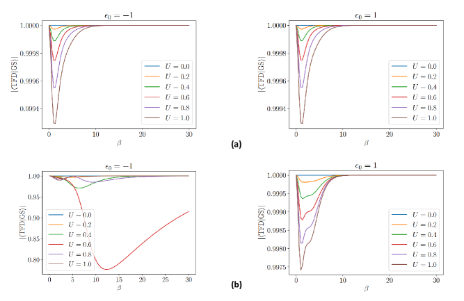
Figure S1: Overlap between the TFD and the GS for the 1D spinless Hubbard model for $\epsilon_{0}=\{-1,1\}$ considering (a) only off-diagonal contributions in the second term of (6), and (b) the full Hamiltonian. The latter case allows interactions to modify the diagonal part, making the non-interacting energies $\omega_{k}$ inefficient in some cases to achieve a good estimation of the weights in $H_{LR}$. In contrast, in (a), the shortened Hubbard term does not modify the $\omega_{k}$, and we can control the deviation from the exact case ($U=0$) through the ratio between $U$ and the hopping constant $t$. Plots show the overlaps for two coupled $N=4$ chains using $t=1$ and varying $U$.

The most natural way is to perform a mean-field approximation in the Hubbard Hamiltonian. That is, treating correlations with the other particles as a mean density and transforming the Hamiltonian into a quadratic one with average densities. The essence of this approximation relies on the fact that density operators $a_{k}^{\dagger}a_{k^{\prime}}$ deviate in a small quantity from their average values $\langle a_{k}^{\dagger}a_{k^{\prime}}\rangle$. Therefore, it is adequate in our case, where we are not interested in strong perturbations to the free fermion regime. It is important to note that we are not using the mean-field approximation to simplify our problem but to estimate correctly the energies, $\omega_{k}(\epsilon_{0},t)\rightarrow\tilde{\omega}_{k}(\epsilon_{0},t,U)=\omega_{k}+\delta\omega_{k}$, from which we generate $H_{LR}$.

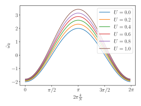
Figure S2: Mean-field energies $\tilde{\omega}_{k}$ (S15) for different values of $U$ and $N=100$.

The mean-field approximation of (S12) gives the following Hamiltonian [23]

$$\begin{split}H^{MF}=\sum_{k}\omega_{k}a_{k}^{\dagger}a_{k}&+\frac{U}{N}\sum_{k,p,q}e^{-i\frac{2\pi}{N}q}a_{k+q}^{\dagger}a_{k}\langle a_{p-q}^{\dagger}a_{p}\rangle+\frac{U}{N}\sum_{k,p,q}e^{-i\frac{2\pi}{N}q}a_{p-q}^{\dagger}a_{p}\langle a_{k+q}^{\dagger}a_{k}\rangle\\ &-\frac{U}{N}\sum_{k,p,q}e^{-i\frac{2\pi}{N}q}\langle a_{k+q}^{\dagger}a_{p}\rangle a_{p-q}^{\dagger}a_{k}-\frac{U}{N}\sum_{k,p,q}e^{-i\frac{2\pi}{N}q}\langle a_{p-q}^{\dagger}a_{k}\rangle a_{k+q}^{\dagger}a_{p}\\ &-\frac{U}{N}\sum_{k,p,q}e^{-i\frac{2\pi}{N}q}\langle a_{k+q}^{\dagger}a_{k}\rangle\langle a_{p-q}^{\dagger}a_{p}\rangle+\frac{U}{N}\sum_{k,p,q}e^{-i\frac{2\pi}{N}q}\langle a_{k+q}^{\dagger}a_{p}\rangle\langle a_{p-q}^{\dagger}a_{k}\rangle\end{split}$$ (S13)

Assuming translational invariance, the average densities can be written as $\langle c^{\dagger}_{k}c_{k}^{\prime}\rangle=\delta_{k.k^{\prime}}\langle n_{k}\rangle$[23]. The odd terms in $q$ cancel in the sums, and the mean-field Hamiltonian turns out to be

$$\begin{split}H^{MF}=\sum_{k}\omega_{k}a_{k}^{\dagger}a_{k}&+\frac{2U}{N}\sum_{k}a_{k}^{\dagger}a_{k}\sum_{p}\langle n_{p}\rangle-\frac{2U}{N}\sum_{k}\cos{\left(\frac{2\pi}{N}k\right)}a_{k}^{\dagger}a_{k}\sum_{p}\cos{\left(\frac{2\pi}{N}p\right)}\langle n_{p}\rangle\\ &-\frac{U}{N}\sum_{k}\langle n_{k}\rangle\sum_{p}\langle n_{p}\rangle+\frac{U}{N}\left(\sum_{k}\cos{\left(\frac{2\pi}{N}k\right)}\langle n_{k}\rangle\right)^{2}\end{split}$$ (S14)

from where the modified energies can be read off

$$\tilde{\omega}_{k}=\omega_{k}+2U\rho-\frac{2U}{N}\cos{\left(\frac{2\pi}{N}k\right)}\sum_{p}\cos{\left(\frac{2\pi}{N}p\right)}\langle n_{p}\rangle$$ (S15)

being $\rho=\frac{N_{e}}{N}=\frac{1}{N}\sum_{p}\langle n_{p}\rangle$ the density of particles. Two equivalent routes can be applied to solve this problem i) determining energies and densities self-consistently $\sum_{k}\langle n_{k}\rangle=\sum_{k}\theta(\mu-\tilde{\omega}_{k})$ or ii) minimizing the free energy with respect to the average densities [23]. In our case, we choose to minimize the energy numerically by finding the optimal configuration [24]. That is, we run over $N_{e}$, filling the $N_{e}$-lowest energy levels, and we identify the lowest energy configuration. Once obtained the modified energies $\tilde{\omega}_{k}$ (Figure S2) we recompute the overlaps , which show, in general, a substantial improvement regarding the case of using the non-interacting energies $\omega_{k}$. Figure S3 shows the numerical results for the previous cases. Finally, note that the overlaps are not invariant under $\epsilon_{0}\rightarrow-\epsilon_{0}$. The reason lies in the density deviations, which depend on $U,t,$ and $\epsilon_{0}$ in different ways. Therefore, the same applies to the limits of what we can consider a weak coupling regime.

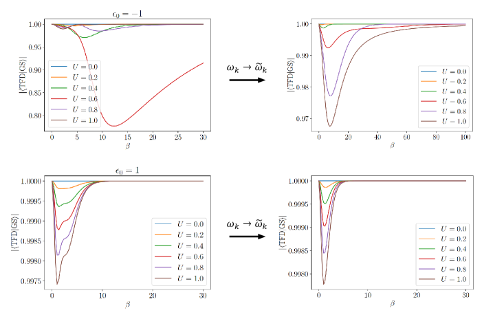
Figure S3: Overlap for the 1D spinless Hubbard model ($\epsilon_{0}=\{-1,1\}$, $t=1$, $2N=8$) using (a) the non-interacting energies $\omega_{k}=\epsilon_{0}-2t\cos{\left(\frac{2\pi}{N}k\right)}$, and (b) their corrected values $\tilde{\omega}_{k}$ within the mean-field approximation.

References

- Watrous [2008] J. Watrous, arXiv preprint arXiv:0804.3401 (2008).
- Aharonov et al. [2013] D. Aharonov, I. Arad, and T. Vidick, Acm sigact news 44, 47 (2013).
- de Vega and Banuls [2015] I. de Vega and M.-C. Banuls, Physical Review A 92, 052116 (2015).
- De Vega and Alonso [2017] I. De Vega and D. Alonso, Reviews of Modern Physics 89, 015001 (2017).
- Tamascelli et al. [2019] D. Tamascelli, A. Smirne, J. Lim, S. F. Huelga, and M. B. Plenio, Physical review letters 123, 090402 (2019).
- Nüßeler et al. [2020] A. Nüßeler, I. Dhand, S. F. Huelga, and M. B. Plenio, Physical Review B 101, 155134 (2020).
- Brown et al. [2023] A. R. Brown, H. Gharibyan, S. Leichenauer, H. W. Lin, S. Nezami, G. Salton, L. Susskind, B. Swingle, and M. Walter, PRX Quantum 4, 010320 (2023), arXiv:1911.06314 [quant-ph] .
- Bhattacharyya et al. [2022] A. Bhattacharyya, L. K. Joshi, and B. Sundar, Eur. Phys. J. C 82, 458 (2022), arXiv:2111.11945 [hep-th] .
- Wu and Hsieh [2019] J. Wu and T. H. Hsieh, Physical review letters 123, 220502 (2019).
- Chowdhury et al. [2020] A. N. Chowdhury, G. H. Low, and N. Wiebe, arXiv preprint arXiv:2002.00055 (2020).
- Sagastizabal et al. [2021] R. Sagastizabal, S. P. Premaratne, B. A. Klaver, M. A. Rol, V. Negîrneac, M. S. Moreira, X. Zou, S. Johri, N. Muthusubramanian, M. Beekman, C. Zachariadis, V. P. Ostroukh, N. Haider, A. Bruno, A. Y. Matsuura, and L. DiCarlo, npj Quantum Information 7, 130 (2021), arXiv:2012.03895 [quant-ph] .
- Wang et al. [2021] Y. Wang, G. Li, and X. Wang, Physical Review Applied 16, 054035 (2021).
- Foldager et al. [2022] J. Foldager, A. Pesah, and L. K. Hansen, Sci. Rep. 12, 3862 (2022), arXiv:2111.03935 [quant-ph] .
- Consiglio et al. [2023] M. Consiglio, J. Settino, A. Giordano, C. Mastroianni, F. Plastina, S. Lorenzo, S. Maniscalco, J. Goold, and T. J. Apollaro, arXiv preprint arXiv:2303.11276 (2023).
- Maldacena and Qi [2018] J. Maldacena and X.-L. Qi, Eternal traversable wormhole (2018), arXiv:1804.00491 .
- Cottrell et al. [2019] W. Cottrell, B. Freivogel, D. M. Hofman, and S. F. Lokhande, Journal of High Energy Physics 2019, 10.1007/jhep02(2019)058 (2019).
- Alet et al. [2021] F. Alet, M. Hanada, A. Jevicki, and C. Peng, Journal of High Energy Physics 2021, 10.1007/jhep02(2021)034 (2021).
- Eddins et al. [2022] A. Eddins, M. Motta, T. P. Gujarati, S. Bravyi, A. Mezzacapo, C. Hadfield, and S. Sheldon, PRX Quantum 3, 010309 (2022).
- Higgott et al. [2019] O. Higgott, D. Wang, and S. Brierley, Quantum 3, 156 (2019).
- Takahashi and Umezawa [1996] Y. Takahashi and H. Umezawa, Int. J. Mod. Phys. B 10, 1755 (1996).
- Surace and Tagliacozzo [2022] J. Surace and L. Tagliacozzo, SciPost Phys. Lect. Notes 54, 1 (2022), arXiv:2111.08343 [quant-ph] .
- Hsieh [2016] T. H. Hsieh, Physical Review B 94, 10.1103/physrevb.94.161112 (2016).
- Bruus and Flensberg [2004] H. Bruus and K. Flensberg, Many-Body Quantum Theory in Condensed Matter Physics: An Introduction, Oxford Graduate Texts (OUP Oxford, 2004).
- Pavarini et al. [2016] E. Pavarini, E. Koch, J. van den Brink, and G. Sawatzky, eds., Quantum Materials: Experiments and Theory, Schriften des Forschungszentrums Jülich. Reihe modeling and simulation, Vol. 6 (Forschungszentrum Jülich GmbH Zentralbibliothek, Verlag, Jülich, 2016) p. 420 S.
- Grover and Rudolph [2002] L. Grover and T. Rudolph, arXiv preprint quant-ph/0208112 (2002).
- Marin-Sanchez et al. [2023] G. Marin-Sanchez, J. Gonzalez-Conde, and M. Sanz, Physical Review Research 5, 033114 (2023).
- Wecker et al. [2015] D. Wecker, M. B. Hastings, and M. Troyer, Phys. Rev. A 92, 042303 (2015).
- Wiersema et al. [2020] R. Wiersema, C. Zhou, Y. de Sereville, J. F. Carrasquilla, Y. B. Kim, and H. Yuen, PRX Quantum 1, 020319 (2020).
- Pachos and Papic [2018] J. Pachos and Z. Papic, SciPost Physics Lecture Notes 10.21468/scipostphyslectnotes.4 (2018).