Worldsheet Formalism for Decoupling Limits in String Theory

Abstract

We study the bosonic sector of a decoupling limit of type IIA superstring theory, where a background Ramond-Ramond one-form is fined tuned to its critical value, such that it cancels the associated background D0-brane tension. The light excitations in this critical limit are D0-branes, whose dynamics are described by Banks-Fischler-Shenker-Susskind (BFSS) Matrix theory that corresponds to M-theory in the Discrete Light-Cone Quantization (DLCQ). We develop the worldsheet formalism for the fundamental string in the same critical limit of type IIA superstring theory. We show that the fundamental string has a nonrelativistic worldsheet, whose topology is described by nodal Riemann spheres as in ambitwistor string theory. We study the T-duality transformations of this string sigma model and provide a worldsheet derivation for the recently revived and expanded duality web that unifies a zoo of decoupling limits in type II superstring theories. By matching the string worldsheet actions, we demonstrate how some of these decoupling limits are related to tensionless (and ambitwistor) string theory, Carrollian string theory, and the Spin Matrix limits of the AdS/CFT correspondence.

1 Introduction and Summary of Main Results

Different vacua in string theory are supposed to be unified by a single M-theory in eleven-dimensions. From the ten-dimensional string theoretical perspective, the extra eleventh dimension corresponds to a large string coupling. The nature of M-theory, which is essentially nonperturbative string theory, still remains mysterious. In certain decoupling limits of string theory where we zoom in on a self-consistent corner such that some states become inaccessible, significant simplification may take place. Such simplifications sometimes allow us to probe nonperturbative aspects of string theory. The classification of such decoupling limits also help us map out different corners in M-theory, which may eventually be assembled into a bigger picture, while being agnostic to what the fundamental principles are.

The studies of various decoupling limits in string/M-theory have been fruitful during the past decades. For example, the renowned AdS/CFT correspondence Maldacena:1997re arises from decoupling the $\mathcal{N}=4$ super Yang-Mills (SYM) theory from IIB supergravity in the string picture and decoupling the near-horizon AdS geometry from the bulk IIB supergravity modes in the $p$-brane picture. This is closely related to the field-theoretical limits of string/M-theory that lead to different effective field theories, including supergravities in the target space, Dirac-Born-Infeld gauge actions on D$p$-branes, and Aharony-Bergman-Jafferis-Maldacena (ABJM) superconformal field theory on M2-branes Aharony:2008ug . Another remarkable decoupling limit that is more relevant to the theme of this paper is the Discrete Light Cone Quantization (DLCQ) of M-theory, i.e. M-theory in spacetime with a lightlike compactification, which is usually achieved by taking a subtle infinite momentum limit along a spacelike circle Susskind:1997cw ; Seiberg:1997ad ; Sen:1997we . In the DLCQ, all light modes except the Kaluza-Klein particle states in the lightlike compactificaion are decoupled, and the theory is described by Banks-Fischler-Shenker-Susskind (BFSS) Matrix quantum mechanics deWit:1988wri ; Banks:1996vh . From the type IIA superstring perspective, the Kaluza-Klein particle states correspond to D0-brane bound states. In the original BFSS paper Banks:1996vh , it is conjectured that BFSS Matrix theory at the large $N$ limit may describe the full nonperturbative M-theory, where $N$ is the size of the matrix. In this large $N$ limit, the Matrix quantum mechanics becomes strongly coupled.

In udlstmt , a duality web surrounding DLCQ M-theory is studied. It is shown that this duality web connects to a zoo of previously studied as well as many new decoupling limits in both type II superstring theory and M-theory. These limits arise from introducing a background brane (or bound branes) with infinite tension, which is canceled by a single (or multiple) $B$-field or Ramond-Ramond (RR) gauge potential that is fine-tuned to its critical value, such that all light excitations except the critical brane states survive. A classic example is BFSS Matrix theory, which can be obtained by starting with type IIA superstring theory with a background D0-brane that is taken to be critical, i.e. the background D0-brane tension is set to infinity and it is canceled by a fine-tuned background RR 1-form (see also Section 2.2). The only remained light excitations are bound D0-brane states described by BFSS Matrix theory. This decoupling limit of type IIA superstring theory is referred to as Matrix 0-brane Theory (M0T) in udlstmt and corresponds to DLCQ M-theory. The target space geometry in M0T is non-Lorentzian, where the conventional Lorentzian boost symmetry being replaced with the Galilean boost symmetry.

In this paper, we develop a worldsheet formalism for the fundamental string in M0T and then study its T-duality transformations. We will focus on the bosonic sector. Unlike the fundamental string in perturbative type IIA superstring theory, the M0T string does not admit any worldsheet wave equations. For this reason, the M0T string is called non-vibrating string in Batlle:2016iel , where the Nambu-Goto and phase space formulations are studied as part of a formal classification of nonrelativistic limits of the string. The fact that the M0T string lacks vibrating modes is not surprising, as the dynamics of M0T is supposed to be captured by the light D0-branes and BFSS Matrix theory instead Banks:1996vh . One may thus question why the fundamental string is of any practical use for us to understand the dynamics of M0T at all. On the contrary, we will show that the M0T string provides a useful tool for mapping out novel decoupling limits of type II string theories via T-duality transformations. We will also show that the worldsheet formalism of the M0T string is closely related to ambitwistor string theory Mason:2013sva ; Geyer:2022cey , where it is possible to compute stringy amplitudes that have localized moduli space and that correspond to particle scatterings.

We will start with a concrete derivation of the M0T string worldsheet action (41) by performing a double dimensional reduction of the M2-brane in DLCQ M-theory, i.e. we compactify the M2-brane by wrapping it around the target space lightlike circle. We will then derive the Polyakov formulation of the M0T string and show that its worldsheet is non-Riemannian. The worldsheet topology of the M0T string is described by the nodal Riemann sphere, which is formed by identifying different pairs of points on a two-sphere. This is reminiscent of the case with a chiral worldsheet, where it is shown that the pairs of nodes on the Riemann sphere correspond to the loops of Feynman diagrams in a quantum field theory (QFT). It has been indicated in that this is more than a coincidence, as ambitwistor string theory is naturally connected to M0T. We will demonstrate this connection explicitly in Section 3.2.2 from the worldsheet perspective. The same worldsheet structure also applies to other corners of type II superstring theories that are connected to M0T via T-duality.

Starting from the M0T string action, we will map out different T-duality transformations of string sigma models and provide a worldsheet derivation for a major part of the duality web of decoupling limits in type II superstring theories that has been outlined in udlstmt , where a road map that schematically depicts the connections between different corners can be found. We highlight the T-dual relations to different decoupling limits in the following list:

1. Matrix theories (Section 3.1 and Fig. 4): We have already explained that BFSS Matrix theory live on the bound D0-brane states in M0T. T-dualizing the M0T string along spatial isometries leads to the fundamental string (96) in the so-called Matrix $p$-brane theory (M$p$T). It is shown in udlstmt that the bound D$p$-branes are the light excitations in M$p$T and they are described by different Matrix gauge theories (also see related discussions in Gopakumar:2000ep ; Harmark:2000ff ; Gomis:2000bd ; Danielsson:2000gi ). In particular, Matrix string theory Dijkgraaf:1997vv is associated with the bound D1-branes in M1T.

2. Tensionless string theory (Section 3.2.1 and Fig. 5): T-dualizing the M0T string along a timelike isometry  leads to the fundamental string (130) in M(-1)T. We show that the M(-1)T string coincides with the Isberg-Lindström-Sundborg-Theodoris (ILST) tensionless limit of the fundamental string in Lindstrom:1990qb ; Isberg:1993av . In M(-1)T, BFSS Matrix theory is T-dualized to Ishibashi-Kawai-Kitazawa-Tsuchiya (IKKT) Matrix theory, which lives on a stack of D(-1)-instantons Ishibashi:1996xs . The target space geometry in M$p$T is non-Lorentzian and is described by generalized Newton-Cartan geometry, which admits Galilei-type instead of Lorentz boost symmetry.

3. Carrollian string theory (Section 3.2.3 and Fig. 5): T-dualizing the M(-1)T string along spatial isometries leads to the fundamental string action (151) that realizes a Carroll-type boost symmetry in the target space, which is described by a generalized Carrollian geometry as in Bergshoeff:2023rkk . These string actions generalize the Carrollian strings in Cardona:2016ytk and connect this previous work to the duality web of decoupling limits. In contrast to Galilean geometry, where the time is absolute but the space transforms into time under the Galilean boost, the space in Carrollian geometry is absolute but the time transforms into space under the Carrollian boost. While Galilean geometry arises from the infinite speed of light limit of Lorentzian geometry, Carrollian geometry arises from the opposite zero speed of light limit levy1965nouvelle ; sen1966analogue ; Duval:2014uoa ; Bergshoeff:2017btm . Such Carrollian strings reside in M$p$T with $p\leq-2$ , whose dynamics is supposedly encoded by Matrix theories on S(pacelike)-branes Hull:1998vg ; Gutperle:2002ai that are T-dual to IKKT Matrix theory. This relation to S-branes, which are localized in time, implies that a Carrollian field theory that live on certain D-branes in M$p$T with $p\leq-2$ might only be defined nonperturbatively. Further studies along these lines may shed light on the pathology in the perturbative quantization of Carrollian field theories Figueroa-OFarrill:2023qty ; deBoer:2023fnj , which may eventually help us understand celestial holography (see e.g. Pasterski:2021raf for a review), in view of its close relation Donnay:2022aba to Carrollian holography.

4. Spin Matrix theory (Section 4.5 and Fig. 7): In M$p$T with $p\neq 0$ , there exists a relativistic sector of the target space where at least one spatial direction is on the same footing as the time. It is therefore possible to form a second DLCQ in M$p$T with $p\neq 0$ . We will show that T-dualizing DLCQ M($p$ +1)T (or M(-$p$ -1)) string action with $p\geq 0$ along the lightlike isometry gives rise to the fundamental string (196) in multicritical Matrix $p$-brane theory (MM$p$T), where the lightlike isometry in M$p$T is mapped to a spacelike (timelike) isometry in MM$p$T. It is shown in udlstmt that MM$p$T arises from a multicritical field limit, where both the background $B$-field and RR $(p+1)$-form are fine-tuned to their critical values, such that they cancel the fundamental string and D$p$-brane tensions in a background bound F1-D$p$ configuration (see also longpaper ). See Section 4 for further details. We will show explicitly in Section 4.5 that the worldsheet action in MM0T matches the string action associated with a Spin Matrix limit of the AdS/CFT correspondence Harmark:2017rpg ; Harmark:2018cdl ; Harmark:2020vll ; Bidussi:2023rfs . In the boundary $\mathcal{N}=4$ SYM, such limit corresponds to a near-BPS limit that leads to a quantum mechanical integrable system called Spin Matrix theories Harmark:2014mpa .

5. Ambitwistor string theory (Section 3.2.2 and Fig. 5; Section 4.6 and Fig. 5): Classically, ambitwistor string theory Mason:2013sva arises from a singular gauge choice in tensionless string theory Casali:2016atr ; Siegel:2015axg . Quantum mechanically, this suggests that one zoom in an unconventional twisted vacuum where creation and annihilation operators are flipped Casali:2016atr ; Bagchi:2020fpr . The quantum amplitudes in ambitwistor string theory reproduce the Cachazo-He-Yuan (CHY) formulae Cachazo:2013hca ; Cachazo:2013iea , which compute field-theoretical amplitudes in the form of string loops. The particle kinematics is encoded by the scattering equations that localize the moduli space of the associated string amplitudes to a set of discrete points (see e.g. Geyer:2015bja for such localizations at loop orders). In the duality map of decoupling limits, the ambitwistor string theory is connected to the M(-1)T string, whose dynamics should be captured by IKKT Matrix theory udlstmt . See more in Section 3.2.2. We will further demonstrate in Section 4.6 that the MM0T string in the ambitwistor string gauge naturally leads to the DLCQ version of the scattering equation, which is potentially useful for constructing CHY formulae for Galilei-invariant field theories.

See udlstmt for a road map that summarizes how the above corners are connected in the duality web. A study from the target space perspective that is complementary to the worldsheet treatment in this paper will appear in longpaper , where the dilaton and RR fields are more accessible. Moreover, connections to Matrix theories, M-theory uplifts and their U-duality relations will also be elaborated therein.

The paper is organized as follows. In Section 2, we start with reviewing the essential ingredients of BFSS Matrix theory in Section 2.1 and then construct the fundamental M0T string action by reducing the M2-brane along a lightlike circle in Section 2.2. We derive the Polyakov formulation of the M0T string in Section 2.3 and show that its worldsheet is non-Riemannian. We then argue that the worldsheet topology is described by nodal Riemann spheres in Section 2.4 and study the symmetries and gauge fixing of the M0T string in Section 2.5. In Section 3, we perform spacelike and timelike T-dualities of the M0T string and provide a worldsheet derivation of the duality web connected to the first DLCQ of M-theory. This duality web connects to Matrix theories, tensionless (and ambitwistor) string theory, and Carrollian string theory as in udlstmt . In Section 4, we consider the lightlike T-duality transformation of M$p$T, which leads to the corners of type II superstring theories in multiple critical background fields udlstmt . We show how MM0T among these corners is related to the Spin Matrix limit of the AdS/CFT correspondence. In Section 5, we provide outlooks for a larger duality web that also involves S-dualities, which have been summarized in udlstmt and will be studied in more detail in longpaper . In appendix A, we present some mathematical detail regarding the worldsheet topology.

2 From Matrix Theory to Fundamental String

In this section, we revisit the corner of type IIA string theory corresponding to M-theory compactified over a lightlike circle. This theory arises from the decoupling limit of IIA where the background RR 1-form is fined tuned to be its critical value and cancels the associated infinite background D0-brane tension, and is referred to as Matrix 1-brane Theory (M1T) in udlstmt . The light states in M1T are D0-branes that are described by BFSS Matrix theory, which we will briefly review. We develop the worldsheet formalism for the fundamental string in M1T and study its target space and worldsheet symmetry. While the target space geometry is non-Lorentzian and is described by Newton-Cartan geometry that covariantizes Newtonian physics, the worldsheet is non-Riemannian, with its topology described by nodal spheres.

2.1 Review of BFSS Matrix Theory

We start with a brief review of BFFS Matrix theory and refer the readers to Taylor:2001vb for further details and references. Historically, Matrix theory arises from the attempt of quantizing the supermembrane in M-theory deWit:1988wri , which is described by a three-dimensional sigma model that maps the supermembrane to eleven-dimensional target spacetime Bergshoeff:1987cm . We denote the membrane worldvolume coordinates by $\sigma^{\alpha}=(\tau,\,\sigma^{1},\,\sigma^{2})$ and denote the target space coordinates by $X^{\text{M}}$ , $\text{M}=0\,,1\,,\cdots\,,10$ . This sigma model is power-counting nonrenormalizable. The Hamiltonian formalism of the membrane simplifies in the light-cone gauge, where we identify the spacetime light-cone direction $X^{-}=\bigl{(}X^{0}-X^{1}\bigr{)}/\sqrt{2}$ with the worldvolume time $\tau$ . However, even under the light-cone gauge condition, the equations of motion from varying the embedding coordinates $X^{\text{M}}$ are still nonlinear, which is different from the situation in string theory and makes the membrane theory difficult to solve. This difficulty from quantizing the supermembrane motivated Goldstone Goldstone:1982 and Hoppe hoppe1987phd to discretize the membrane surface by using a “matrix regularization,” where functions on the membrane surface are regularized to be $N\times N$ matrices. It was later shown in deWit:1988wri that the quantized supermembrane in the matrix regularization is described by the Hamiltonian baake1985fierz ; flume1985quantum ; Claudson:1984th ,

$$H=\frac{1}{2\,g^{2}}\,\text{tr}\Bigl{(}\partial_{\tau}X^{i}\,\partial_{\tau}X^{i}-\tfrac{1}{2}\,\bigl{[}X^{i},\,X^{j}\bigr{]}\,\bigl{[}X^{i},\,X^{j}\bigr{]}+\psi^{\intercal}\,\gamma^{i}\,\bigl{[}X^{i},\,\psi\bigr{]}\Bigr{)}\,,$$ (1)

where $X^{i}$ , $i=2\,,\cdots\,,10$ are $N\times N$ matrices, $\psi$ is a 16-component Matrix-valued spinor of SO$(9)$ , and $\gamma^{i}$ are the SO$(9)$ Dirac matrices in the 16-dimensional representation. The Hamiltonian (1) describes an $\mathcal{N}=16$ supersymmetric quantum mechanical theory with matrix degrees of freedom, which is referred to as the Banks-Fischler-Shenker-Susskind (BFSS) Matrix theory. However, BFFS Matrix theory does not describe a single first-quantized membrane, which is prone to creating long thin spikes at a cost of negligible energy and is thus unstable deWit:1988xki . Instead, the action (1) describes a “second-quantized” theory with a continuous spectrum. This important multi-particle interpretation was pioneered in Banks:1996vh . Heuristically, this is because the continuous large $N$ limit of the discretized membrane surface in the matrix regularization does not necessarily lead to a single membrane anymore.

There is a rather significant connection between BFSS Matrix theory and the low-energy description of the bound state of $N$ D0-branes in type IIA superstring theory Townsend:1995af . The action (1) is identical to the dimensional reduction of ten-dimensional SYM theory to (0+1)-dimensions Witten:1995im . The ten-dimensional SYM arises from a zero Regge slope (field theory) limit of a stack of $N$ D9-branes in type IIA superstring theory. On the other hand, the dimensional reduction is equivalent to performing T-duality transformations along all the spatial directions of the stack of D9-branes, which gives rise to a bound state of $N$ D0-branes. Therefore, in the T-dual frame of the zero-Regge slope limit of the D9-branes, the bound state of D0-branes is described by the nonrelativistic quantum mechanical system.

Based on the above observations, it is argued in Susskind:1997cw ; Seiberg:1997ad ; Sen:1997we that the Matrix theory (1) at finite $N$ describes M-theory in spacetime with a lightlike compactification, where $N$ is the Kaluza-Klein (KK) momentum number in the lightlike circle. Such KK modes in the M-theory circle correspond to the bound D0-brane states in type IIA superstring theory. Compactifying M-theory over a lightlike circle is what we refer to as the Discrete Light Cone Quantization (DLCQ) of M-theory. In the large $N$ limit, the lightlike circle decompactifies and DLCQ M-theory is related to M-theory in the infinite momentum frame, whose dynamics was famously conjectured to be described by the large $N$ limit of the BFSS Matrix theory (1) Banks:1996vh .

2.2 Critical Ramond-Ramond One-Form Limit

Now, we formulate explicitly the decoupling limit of type IIA superstring theory under which BFSS Matrix theory arises. In this decoupling limit, a background 1-form RR potential is fined tuned to be critical and cancels the background D0-brane tension. We will first derive the fundamental string and D2-brane action from compactifying a single M2-brane in eleven-dimensional spacetime over a lightlike circle, i.e. DLCQ M-theory.  We will then derive the appropriate critical RR 1-form limit of the associated string and brane objects in the IIA theory, such that the dimensionally reduced actions are reproduced. This limiting procedure matches the ones considered in Gopakumar:2000ep ; Harmark:2000ff ; Gomis:2000bd ; Danielsson:2000gi ; udlstmt . The connection between DLCQ M-theory and BFSS Matrix theory guarantees that the latter arises from the same critical limit when applied to a stack of D0-branes in the IIA theory. We refer the readers to longpaper for an explicit derivation of BFSS Matrix theory from directly applying the limit to D0-branes. We will focus on the bosonic sector but with arbitrary background fields.

$\bullet$ M2-brane in the DLCQ. We start with M-theory in the eleven-dimensional target space $\mathcal{M}_{11}$ with a lightlike isometry, and consider a single M2-brane coupled to the M-theory metric and three-form gauge background field. Define the worldvolume coordinates on the M2-brane manifold $\Sigma_{3}$ to be $\sigma^{\alpha}$ , $\alpha=0\,,1\,,2$ , and define the embedding coordinates that map $\Sigma_{3}$ to $\mathcal{M}_{11}$ to be $X^{\text{M}}$ , $\text{M}=0\,,1\,,\cdots\,,10$ . Furthermore, in the coordinate system adapted to the lightlike isometry $\theta$ , the spacetime coordinates are $x^{M}=(x^{\mu},\Theta)$ , with $\mu=0\,,1\,,\cdots\,,9$ . Define the first fundamental form on $\mathcal{M}_{11}$ to be

$$ds^{2}_{11}=2\,\mathbb{G}_{\mu\Theta}\,dx^{\mu}\,d\Theta+\mathbb{G}_{\mu\nu}\,dx^{\mu}\,dx^{\nu}\,.$$ (2)

Note that $\mathbb{G}_{\Theta\Theta}=0$ because $\Theta$ is the lightlike direction. The classical M2-brane action is given by the three-dimensional worldvolume action Bergshoeff:1987cm ,

$$S_{\text{M2}}=-T_{\text{M2}}\int d^{3}\sigma\,\sqrt{-\det\Bigl{(}\partial_{\alpha}X^{\text{M}}_{\phantom{\dagger}}\,\partial_{\beta}X^{\text{N}}_{\phantom{\dagger}}\,\mathbb{G}_{\text{MN}}\Bigr{)}}+T_{\text{M2}}\int\mathbb{C}^{(3)}\,,$$ (3)

where $\mathbb{C}^{(3)}$ is the three-form gauge potential being pulled back from $\mathcal{M}_{11}$ to $\Sigma_{3}$ . Define the frame field $\mathbb{E}_{\text{M}}{}^{\mathbb{A}}$ via $\mathbb{G}_{\text{MN}}=\mathbb{E}_{\text{M}}{}^{\mathbb{A}}\,\mathbb{E}_{\text{N}}{}^{\mathbb{B}}\,\eta_{\mathbb{A}\mathbb{B}}$ , $\mathbb{A}=0\,,1\,,\cdots\,,10$ , and define the associated lightlike components to be

$$\mathbb{E}^{+}=\frac{1}{\sqrt{2}}\,\bigl{(}\mathbb{E}^{0}+\mathbb{E}^{10}\bigr{)}\,,\qquad\mathbb{E}^{-}=\frac{1}{\sqrt{2}}\,\bigl{(}\mathbb{E}^{0}-\mathbb{E}^{10}\bigr{)}\,.$$ (4)

The lightlike Kaluza-Klein reduction ansatze are

$$\mathbb{E}_{\Theta}{}^{+} =0\,, \mathbb{E}_{\Theta}{}^{-} =e^{2\Phi/3}\,, \mathbb{E}_{\Theta}{}^{A^{\prime}} =0\,,$$ (5a)

$$\mathbb{E}_{\mu}{}^{+} =e^{-\Phi/3}\,\tau_{\mu}{}^{0}\,, \mathbb{E}_{\mu}{}^{-} =e^{2\Phi/3}\,C_{\mu}\,, \mathbb{E}_{\mu}{}^{A^{\prime}} =e^{-\Phi/3}\,E_{\mu}{}^{A^{\prime}},$$ (5b)

where $\tau_{\mu}{}^{0}$ and $E_{\mu}{}^{A^{\prime}}$, $A^{\prime}=1\,,\cdots\,,9$ are vielbein fields in the resulting type IIA superstring theory and $C^{(1)}=C_{\mu}\,dx^{\mu}$ is the RR 1-form. Moreover, $\mathbb{C}_{\mu\nu\rho}=C_{\mu\nu\rho}$ and $\mathbb{C}_{\mu\nu\Theta}=-B_{\mu\nu}$ are the associated RR three-form and $B$-field, respectively. In terms of the adapted coordinates and of the metric in Eq. (2), we find that the action (3) becomes

$$\begin{split}S_{\text{M2}}=&-T_{\text{M2}}\int d^{3}\sigma\,e^{-\Phi}\,\sqrt{-\det\Bigl{[}-e^{\Phi}\,\bigl{(}\tau_{\alpha}{}^{0}\,D_{\!\beta}\Theta+\tau_{\beta}{}^{0}\,D_{\!\alpha}\Theta\bigr{)}+E_{\alpha\beta}\Bigr{]}}\\[4.0pt] &+T_{\text{M2}}\int\Bigl{(}C^{(3)}-B\wedge\Theta^{(1)}\Bigr{)}\,,\end{split}$$ (6)

where $E_{\mu\nu}=E_{\mu}{}^{A^{\prime}}\,E_{\nu}{}^{A^{\prime}}$, $D_{\!\alpha}\Theta=\partial_{\alpha}\Theta+C_{\alpha}$ and $\Theta^{(1)}=d\Theta$ . We have introduced the pullbacks with $\mathcal{T}_{\alpha}=\partial_{\alpha}X^{\mu}\,\mathcal{T}_{\mu}$ for any tensor $\mathcal{T}_{\mu}$ .

$\bullet$ Double dimensional reduction. Next, we perform different dimensional reductions of the M2-brane action (6) to probe the physical contents of the associated string theory in ten-dimensions. First, we consider a double dimensional reduction of Eq. (6), where the M2-brane is wrapped over the lightlike M-theory circle. This amounts to identify $\Theta=\sigma^{2}$ and to require that the background fields together with the embedding coordinates $x^{\mu}$ be independent of $\Theta$ . We find the following fundamental string action:

$$S_{\text{F1}}=-T\int d^{2}\sigma\,\sqrt{-\mathcal{M}}-T\int B\,,\qquad\mathcal{M}=\det\begin{pmatrix}0&\,\,\tau_{\beta}{}^{0}\\[4.0pt] \tau_{\alpha}{}^{0}&\,\,E_{\alpha\beta}\end{pmatrix},\,\,\alpha=0\,,1\,.$$ (7)

The action (7) describes the fundamental string in a non-Lorentzian target space geometry, encoded by the time vielbein field $\tau_{\mu}$ and spatial vielbein field $E_{\mu}{}^{A^{\prime}}$, $A^{\prime}=1,\cdots,9$ , which are related via a Galilean boost transformation parametrized by the boost velocity $\Lambda^{A^{\prime}}$,

$$\delta_{\text{G}}\tau^{0}=0\,,\qquad\delta_{\text{G}}E^{A^{\prime}}=\Lambda^{A^{\prime}}\,\tau^{0}\,.$$ (8)

Note that Eq. (7) is manifestly invariant under the Galilean boost (8). The vielbein fields $\tau^{0}$ and $E^{A^{\prime}}$ describe Newton-Cartan geometry that geometrizes Newtonian gravity. The target space has an absolute time direction defined by $\tau^{0}$ and an SO(9) rotation symmetry in the spatial slice. In flat target sapce with $\tau_{\mu}{}^{0}=\delta_{\mu}^{0}$ and $E_{\mu}{}^{A^{\prime}}=\delta_{\mu}^{A^{\prime}}$, the action (7) reduces to the non-vibrating string studied in Batlle:2016iel .

$\bullet$ Direct dimensional reduction. We will show momentarily that the fundamental string described by Eq. (9) lives in the critical RR 1-form limit of type IIA superstring theory, where $C^{(1)}$ becomes critical udlstmt . However, the input from the fundamental string action (7) is not sufficient for us to access the RR sector. In order to probe the RR sector, we now consider a direct dimensional reduction of the M2-brane action (6). Following the strategy in Townsend:1996xj , we dualize $\Theta$ in Eq. (6) and find the following D2-brane action:

$$S_{\text{D2}} =-\frac{T_{\text{D2}}}{2}\int d^{3}\sigma\,\frac{\det\mathcal{M}+\widetilde{\mathcal{F}}^{\alpha}\,E_{\alpha\beta}\,\widetilde{\mathcal{F}}^{\beta}}{e^{\varphi}\,\text{tr}\Bigl{(}\widetilde{\mathcal{F}}^{\gamma}_{\phantom{\dagger}}\,\tau_{\gamma}{}^{0}\Bigr{)}}+T_{\text{D2}}\int\Bigl{(}C^{(3)}+C^{(1)}\wedge\mathcal{F}\Bigr{)}\,,$$ (9)

where $\mathcal{F}=B+F$ , with $F=dA$ the $U(1)$ gauge field strength, and $\widetilde{\mathcal{F}}^{\alpha}=\frac{1}{2}\,\epsilon^{\alpha\beta\gamma}\mathcal{F}_{\beta\gamma}$ . We have chosen $\text{tr}\bigl{(}\widetilde{\mathcal{F}}{}^{\alpha}\,\tau_{\alpha}{}^{0}\bigr{)}<0$ . The action (9) describes a single D2-brane in Newton-Cartan geometry. This D2-brane action may appear to be exotic, but it will become manifest after we derive the prescriptions for implementing the critical RR 1-form limit in the IIA theory. We will come back to comment on this brane action (9) at the end of this subsection.

$\bullet$ Critical RR 1-form limit. Now, we are ready to construct the appropriate decoupling limit by requiring that Eqs. (7) and (9) arise from an $\omega\rightarrow\infty$ limit of the fundamental string and D2-brane action, respectively, in type IIA superstring theory, whose background fields we denote using a hatted notation,

$$\hat{S}_{\text{F1}} =-T\int d^{2}\sigma\,\sqrt{-\det\hat{G}_{\alpha\beta}}-T\int\hat{B}\,,$$ (10a)

$$\hat{S}_{\text{D2}} =-T_{\text{D2}}\int d^{3}\sigma\,e^{-\hat{\Phi}}\sqrt{-\det\Bigl{(}\hat{G}_{\alpha\beta}+\hat{\mathcal{F}}_{\alpha\beta}\Bigr{)}}+T_{\text{D2}}\int\Bigl{(}\hat{C}^{(3)}+\hat{C}^{(1)}\wedge\hat{\mathcal{F}}\Bigr{)}.$$ (10b)

Consider the ansatze relating the ingredients in Eqs. (10) to Eqs. (7) and (9) below:

$$\hat{G}_{\mu\nu}=-\omega\,\tau_{\mu}{}^{0}\,\tau_{\nu}{}^{0}+\omega^{\sigma_{\!\text{\scalebox{0.8}{$E$}}}}E_{\mu\nu}\,,\qquad\hat{\mathcal{F}}=\omega^{\sigma_{\!\text{\scalebox{0.8}{$\mathcal{F}$}}}}\mathcal{F}\,,\qquad\hat{\Phi}=\Phi+\sigma_{\!\text{\scalebox{0.8}{$\Phi$}}}\ln\omega\,.$$ (11)

Without loss of generality, we fixed the exponent of $\omega$ in front of the $\tau_{\mu}{}^{0}$ term in $\hat{G}_{\mu\nu}$ to be unit. Requiring that Eq. (10) give Eqs. (7) and (9) at $\omega\rightarrow\infty$ uniquely imposes $(\sigma_{\text{\scalebox{0.8}{$E$}}}\,,\sigma_{\text{\scalebox{0.8}{$\mathcal{F}$}}}\,,\sigma_{\text{\scalebox{0.8}{$\Phi$}}})=(-1\,,0\,,-3/2)$ and

$$\hat{G}_{\mu\nu} =-\omega\,\tau_{\mu}{}^{0}\,\tau_{\nu}{}^{0}+\omega^{-1}\,E_{\mu\nu}\,,\qquad\hat{\Phi}=\Phi-\frac{3}{2}\ln\omega\,,$$ (12a)

$$\hat{C}^{(1)} =\omega^{2}\,e^{-\Phi}\,\tau^{0}+C^{(1)}\,,\qquad\quad\hat{C}^{(3)}=C^{(3)}\,,\qquad\hat{B}=B\,.$$ (12b)

These prespecriptions match udlstmt . Also see Gopakumar:2000ep for the same prescription in flat target space. Recall that we had to require $\text{tr}\bigl{(}\widetilde{\mathcal{F}}^{\alpha}_{\phantom{\dagger}}\,\tau_{\alpha}{}^{0}\bigr{)}<0$ for the divergences in $\omega$ to be canceled in the D2-brane action. This choice of branch is associated with the choice of the sign in front of the $\omega$ divergence in $\hat{C}^{(1)}$ in Eq. (12b), which is reminiscent of the IIB case in the critical $B$-field limit in Bergshoeff:2022iss . It is also expected that $\hat{C}^{(q)}=C^{(q)}$ for $q\neq 1$ ; see longpaper for a rigorous derivation for these prescriptions including Eq. (12). Reparametrizing the (bosonic) background fields in type IIA superstring theory as in Eq. (12), sending $\omega$ to infinity defines the desired critical RR 1-form limit.

Applying this limit to the nonabelian Dirac-Born-Infeld action describing a stack of relativistic D0-branes in type IIA superstring theory reproduces BFSS Matrix theory (1), confirming its correspondence to DLCQ M-theory. We briefly review how this works udlstmt ; longpaper . Consider the nonabelian effective action Myers:1999ps of a stack of $N$ coinciding relativistic D0-branes,

$$S_{\text{D0}}=-\frac{T_{1}}{2}\int d^{p+1}\sigma\,e^{-\Phi}\,\text{tr}\sqrt{\Bigl{(}-\partial_{\tau}X^{\mu}_{\phantom{\dagger}}\,\partial_{\tau}X_{\mu}\Bigr{)}\,\det\Bigl{(}\delta^{i}_{j}+i\,\bigl{[}X^{i},\,X_{j}\bigr{]}\Bigr{)}}\,.$$ (13)

which is supplemented with the appropriate Chern-Simons terms that contain various RR potentials. Here, $X^{i}$ are scalars in the adjoint representation of $U(N)$ . We require that $\Phi$ is constant and take static gauge $X^{0}=\tau$ . Plugging Eq. (12) into the D0-brane action (13) and including the $\omega^{2}$ piece from the RR 1-form in the Chern-Simons term, we recover the bosonic part of BFSS Matrix theory (1) in the $\omega\rightarrow\infty$ limit. In view of this connection to Matrix theory, the critical RR 1-form limit of type IIA superstring theory is referred to as Matrix 0-brane Theory (M0T) in udlstmt .

$\bullet$ Non-Commutative Yang-Mills on D2-branes. We now return to the physics of the D2-brane action (9), which turns out to be T-dual to four-dimensional Non-Commutative Yang-Mills (NCYM) Gopakumar:2000na . In fact, the gauge theory on the a stack of $N$ M0T D2-brane is three-dimensional NCYM, such that the two spatial directions on the D2-brane do not commute with each other. We demonstrate this for a single M0T D2-brane below. In flat target space and in static gauge with $\tau_{\alpha}{}^{0}=\delta_{\alpha}^{0}$ and $E_{\alpha\beta}=\text{diag}(0\,,1\,,1)$ , the vacuum expectation value of $\text{tr}\bigl{(}\widetilde{\mathcal{F}}^{\alpha}_{\phantom{\dagger}}\,\tau_{\alpha}{}^{0}\bigr{)}$ that appears as a denominator in Eq. (9) is $B_{12}$ , where the gauge mode $A_{\mu}$ is treated as a fluctuation over a $B$-field background. This $B_{12}$ has to be nonzero for the action (9) to be well defined and acts as the source of spatial noncommutativity on the D2-brane. This noncommutative behavior can be made manifest by applying the Seiberg-Witten map Seiberg:1999vs to transform the closed string data to the effective background fields seen by the open strings. In particular, the open-string background field measuring the noncommutativity between the D2-brane worldvolume coordinates in type IIA superstring theory is

$$\hat{\Theta}^{\alpha\beta}=-\Bigl{[}\bigl{(}\hat{G}+\hat{B}\bigr{)}^{-1}\hat{B}\,\bigl{(}\hat{G}+\hat{B}\bigr{)}^{-1}\Bigr{]}^{\alpha\beta}.$$ (14)

Plug Eq. (12) into Eq. (14), with

$$\hat{G}=\begin{pmatrix}-\omega&\,\,\,\,0&\,\,0\\[4.0pt] 0&\,\,\,\,\omega^{-1}&\,\,0\\[4.0pt] 0&\,\,\,\,0&\,\,\omega^{-1}\end{pmatrix}\,,\qquad\hat{B}=\begin{pmatrix}\,0&\,\,\,\,0&\,\,0\\[4.0pt] \,0&\,\,\,\,0&\,\,B_{12}\\[4.0pt] \,0&\,\,\,\,-B_{12}&\,\,0\end{pmatrix},$$ (15)

the $\omega\rightarrow\infty$ limit gives

$$\hat{\Theta}^{\alpha\beta}=B_{12}^{-1}\begin{pmatrix}\,0&\,\,0&\,\,0\,\\[2.0pt] \,0&\,\,0&\,\,1\,\\[2.0pt] \,0&\,\,-1&\,\,0\,\end{pmatrix},$$ (16)

which implies $[\sigma^{1},\,\sigma^{2}]\sim B_{12}^{-1}$ , i.e., the Kalb-Ramond field $B_{12}$ controls the noncommutativity between the spatial directions on the D2-brane. The open string coupling $\hat{g}_{\text{o}}$ is given by

$$\hat{g}^{2}_{\text{o}}=e^{\hat{\Phi}}\,\sqrt{\frac{\det\bigl{(}\hat{G}_{\alpha\beta}+\hat{B}_{\alpha\beta}\bigr{)}}{\det\hat{G}_{\gamma\delta}}}=\omega^{-1/2}\,g_{\text{o}}^{2}+O(\omega^{-5/2})\,,\qquad g_{\text{o}}^{2}=e^{\Phi}\,|B_{12}|\,,$$ (17)

which shows that, in the $\omega\rightarrow\infty$ limit, the effective gauge coupling $g_{\text{o}}$ in NCYM is controlled by the vacuum expectation value of $e^{\Phi/2}\sqrt{|B_{12}|}$ .

2.3 Fundamental String in Matrix 0-Brane Theory

We now turn our attention to the fundamental string action (7). In Matrix 0-brane Theory (M0T), the light excitations are bound states of nonrelativistic D0-branes instead of the fundamental string in perturbative string theory. The D0-brane dynamics is described by BFSS Matrix theory. However, as we have seen in Section 2.2, the M0T D2-branes also carry nontrivial NCYM dynamics in the presence of a nonzero magnetic $B$-field on the worldvolume. It is interesting to study the fundamental string in M0T for a different reason. As we will see later in Section 2.5, the M0T fundamental string does not vibrate; nevertheless, as we will demonstrate through the rest of the paper, the worldsheet formalism of the M0T string provides a useful worldsheet tool for mapping out different decoupling limits by classifying T-duality transformations of the M0T fundamental string sigma models.

$\bullet$ Nambu-Goto action. We start with a derivation of the M0T string action (7) by explicitly performing the critical RR 1-form of the string action (10a) in type IIA superstring theory. Plugging Eq. (12) into Eq. (10a), we find

$$\hat{S}_{\text{F1}}=-T\int d^{2}\sigma\,\sqrt{-\omega^{-2}\,\det\Bigl{(}E_{\alpha\beta}-\omega^{2}\,\tau_{\alpha}{}^{0}\,\tau_{\beta}{}^{0}\Bigr{)}}-T\int B\,,$$ (18)

Note the following identity of block matrices:

$$\det\begin{pmatrix}M_{1}&\,\,M_{2}\\[4.0pt] M_{3}&\,\,M_{4}\end{pmatrix}=\Bigl{(}\det M_{1}\Bigr{)}\,\det\Bigl{(}M_{4}-M_{3}\,M_{1}^{-1}\,M_{2}\Bigr{)}\,.$$ (19)

Assume that $M_{1}\!=\!\omega^{-2}$, $M_{2}^{\intercal}\!=\!M_{3}\!=\!\bigl{(}\tau_{\alpha}{}^{0}\bigr{)}$ , and $M_{4}\!=\!\bigl{(}E_{\alpha\beta}\bigr{)}$ , we find that Eq. (18) becomes

$$\hat{S}_{\text{F1}}=-T\int d^{2}\sigma\,\sqrt{-\det\begin{pmatrix}\omega^{-2}&\,\,\tau_{\beta}{}^{0}\\[4.0pt] \tau_{\alpha}{}^{0}&\,\,E_{\alpha\beta}\end{pmatrix}}-T\int B\,.$$ (20)

In the $\omega\rightarrow\infty$ limit, we find that Eq. (20) reduces to the M0T string action (7).

$\bullet$ Phase space action. Before we construct the Polyakov action that is equivalent to the Nambu-Goto action (7), it is instructive to first consider the phase space formulation. For simplicity, we set the $B$-field to zero in the following derivation. In terms of the worldsheet coordinates $\sigma^{\alpha}=(\tau,\sigma)$ , the phase space action is

$$S_{\text{p.s.}}=\int d^{2}\sigma\,\biggl{\{}P_{\mu}\,\partial_{\tau}X^{\mu}-\frac{\chi}{2\,T}\Bigl{[}P_{\mu}\,E^{\mu\nu}\,P_{\nu}-T^{2}\,\bigl{(}\partial_{\sigma}X^{\mu}\,\tau_{\mu}{}^{0}\bigr{)}^{2}\Bigr{]}-\rho\,P_{\mu}\,\partial_{\sigma}X^{\mu}\biggr{\}}\,,$$ (21)

which generalizes the result in Batlle:2016iel to curved background fields. Here, $P_{\mu}$ is the conjugate momentum associated with the generalized coordinates $X^{\mu}$. Moreover, $E^{\mu\nu}=E^{\mu}{}_{A^{\prime}}\,E^{\nu}{}_{\!A^{\prime}}$ , with the inverse vielbein fields $E^{\mu}{}_{\!A^{\prime}}$ (and $\tau^{\mu}{}_{0}$) defined via the orthogonality conditions,

$$\tau^{\mu}_{0}\,\tau_{\mu}{}^{0} =1\,, \tau_{\mu}{}^{0}\,\tau^{\nu}_{0}+E_{\mu}{}^{A^{\prime}}\,E^{\nu}_{A^{\prime}} =\delta_{\mu}^{\nu}\,,$$ (22a)

$$E^{\mu}_{\!A^{\prime}}\,E_{\mu}{}^{B^{\prime}} =\delta_{A^{\prime}}^{B^{\prime}}\,, \tau^{\mu}_{0}\,E_{\mu}{}^{A^{\prime}}=E^{\mu}_{\!A^{\prime}}\,\tau_{\mu}{}^{0} =0\,.$$ (22b)

The Lagrange multipliers $\chi$ and $\rho$ impose the Hamiltonian constraints. Integrating out $P_{\mu}$ , $\rho$ , and $\chi$ in Eq. (21) gives back the Nambu-Goto action (7).

We now discuss how to obtain (21) from taking the critical RR 1-form limit of the phase space action of the conventional string,

$$\hat{S}_{\text{p.s.}}=\int d^{2}\sigma\,\biggl{[}P_{\mu}\,\partial_{\tau}X^{\mu}-\frac{\hat{\chi}}{2\,T}\Bigl{(}P_{\mu}\,P_{\nu}\,\hat{G}^{\mu\nu}+T^{2}\,\hat{G}\,\hat{G}^{\tau\tau}\Bigr{)}-\hat{\rho}\,P_{\mu}\,\partial_{\sigma}X^{\mu}\biggr{]},$$ (23)

where $\hat{G}^{\tau\tau}$ is a component of the inverse $\hat{G}^{\alpha\beta}$ of the pullback $\hat{G}_{\alpha\beta}$ . Integrating out $P_{\mu}$ , $\hat{\rho}$ , and $\hat{\chi}$ in Eq. (23) gives back the Nambu-Goto action (10a). Using the reparametrization of $\hat{G}_{\mu\nu}$ in Eq. (12a), and requiring that Eq. (21) arise from the $\omega\rightarrow\infty$ limit of Eq. (23), we derive the following prescription for $\hat{\chi}$ and $\hat{\rho}$ :

$$\hat{\chi}=\omega^{-1}\,\chi+O\bigl{(}\omega^{-3}\bigr{)}\,,\qquad\hat{\rho}=\rho+O\bigl{(}\omega^{-2}\bigr{)}\,.$$ (24)

These relations between the Lagrange multipliers imposing the Hamiltonian constraints in the phase space action will play an important role for us to understand the M0T string worldsheet geometry, which becomes nonrelativistic.

$\bullet$ Nonrelativistic worldsheet. To pass from the phase space action (23) to its Polyakov action for the conventional string, we introduce the worldsheet zweibein field $\hat{e}_{\alpha}{}^{a}$ , $a=0\,,1$ and write

$$\hat{\chi}=\frac{\hat{e}}{\hat{h}_{\sigma\sigma}}\,,\qquad\hat{\rho}=\frac{\hat{h}_{\tau\sigma}}{\hat{h}_{\sigma\sigma}}\,,\qquad\hat{e}=\det\bigl{(}\hat{e}_{\alpha}{}^{a}\bigr{)}\,,\qquad\hat{h}_{\alpha\beta}=e_{\alpha}{}^{a}\,e_{\beta}{}^{b}\,\eta_{ab}\,.$$ (25)

Integrating out $P_{\mu}$ in Eq. (23) yields the standard Polyakov action,

$$\hat{S}_{\text{P}}=-\frac{T}{2}\int d^{2}\sigma\,\sqrt{-\hat{h}}\,\hat{h}^{\alpha\beta}\,\partial_{\alpha}X^{\mu}\,\partial_{\beta}X^{\nu}\,\hat{G}_{\mu\nu}-T\int\hat{B}\,,$$ (26)

with the worldsheet metric $\hat{h}_{\alpha\beta}$ . Here, we have reintroduced the $B$-field dependence. In order to achieve the rescaling in Eq. (24), we adopt the following reparametrizations:

$$\hat{e}_{\alpha}{}^{0}=\Omega\,\omega^{z}\,e_{\alpha}{}^{0}\,,\qquad\hat{e}_{\alpha}{}^{1}=\Omega\,e_{\alpha}{}^{1}\,,$$ (27)

where $\Omega$ is a conformal factor that we set to one and the exponent $z$ is to be determined. Matching Eq. (25) with Eq. (24), we find $|z|=1$ , in which cases the worldsheet metric becomes singular in the $\omega\rightarrow\infty$ limit and the resulting worldsheet geometry does not admit any metric description and is therefore nonrelativistic. Instead, the worldsheet geometry is only appropriately described by the vielbein fields $e_{\alpha}{}^{0}$ and $e_{\alpha}{}^{1}$ . We discuss both the $z=\pm 1$ cases below:

1. Galilean Worldsheet. When $z=1$ , we have

   $$\chi=\frac{e}{\bigl{(}e_{\sigma}{}^{0}\bigr{)}^{2}}\,,\qquad\rho=\frac{e_{\tau}{}^{0}}{e_{\sigma}{}^{0}}\,,\qquad e=\det e_{\alpha}{}^{a}\,,$$ (28)

   and

   $$\hat{h}_{\alpha\beta}=-\omega^{2}\,e_{\alpha}{}^{0}\,e_{\beta}{}^{0}+e_{\alpha}{}^{1}\,e_{\beta}{}^{1}\,.$$ (29)

   The worldsheet becomes Galilean in the $\omega\rightarrow\infty$ limit, with the vielbein fields related via the Galilean boost,

   $$\delta_{\text{g}}e^{0}=0\,,\qquad\delta_{\text{g}}e^{1}=v\,e^{0}\,,$$ (30)

   which arises from the $\omega\rightarrow\infty$ limit of the Lorentz boost. The Levi-Civita symbol $\epsilon_{ab}$ is defined via $\epsilon_{01}=1$ and the indices are raised (or lowered) by a Minkowski metric. Define $t=e^{0}$ and $x=e^{1}$, we bring the infinitesimal Galilean boost transformation (30) to the finite form as $t\rightarrow t$ and $x\rightarrow x+v\,t$ , which of course comes from sending the speed of light $c$ to infinity in the Lorentz boost

   $$t\rightarrow\frac{t+\frac{v}{c^{2}}\,x}{\sqrt{1-\frac{v^{2}}{c^{2}}}}\,,\qquad x\rightarrow\frac{x+v\,t}{\sqrt{1-\frac{v^{2}}{c^{2}}}}\,.$$ (31)

2. Carrollian Worldsheet. When $z=-1$ , we have

   $$\chi=\frac{e}{\bigl{(}e_{\sigma}{}^{1}\bigr{)}^{2}}\,,\qquad\rho=\frac{e_{\tau}{}^{1}}{e_{\sigma}{}^{1}}\,,$$ (32)

   and

   $$\hat{h}_{\alpha\beta}=-\omega^{-2}\,e_{\alpha}{}^{0}\,e_{\beta}{}^{0}+e_{\alpha}{}^{1}\,e_{\beta}{}^{1}\,,$$ (33)

   where, in the $\omega\rightarrow\infty$ limit, the vielbein fields are related via a different boost,

   $$\delta_{\text{c}}e^{0}=\beta\,e^{1},\qquad\delta_{\text{c}}e^{1}=0\,.$$ (34)

   This is the so-called Carrollian boost, which arises from sending both $v$ and $c$ in the Lorentz boost transformation (31) to zero while keeping $\beta\equiv v/c^{2}$ finite, such that Eq. (31) becomes $t\rightarrow t+\beta\,x$ and $x\rightarrow x$ . In this sense, we say that the worldsheet geometry is Carrollian, where the space is absolute while the time is relative. This is in contrast to the Galilean case, where the time is absolute while the space is relative.

After Wick rotating the worldsheet time, the choices (29) and (33) are equivalent to each other on the two-dimensional Euclidean manifold, up to a conformal factor. However, the Schild (or transverse) gauge

$$\chi=1\,,\qquad\rho=0\,.$$ (35)

appears to be more natural in the Carrollian parametrization (32) of the worldsheet, where it simply translates to the conformal gauge $e_{\alpha}{}^{a}\propto\delta_{\alpha}^{a}$ . In contrast, the Schild gauge is associated with setting $e_{\alpha}{}^{b}\,\epsilon_{b}{}^{a}=\delta_{\alpha}^{a}$ in the Galilean parametrization (28) of the worldsheet.

We will mostly use the Carrollian worldsheet but will also resort to the Galilean worldsheet when we discuss the Spin Matrix theory later in Section 4.5. It is straightforward to go between the Galilean and Carrollian parametrizations of the worldsheet by using the mapping

$$e^{0}\rightarrow i\,e^{1}\,,\qquad e^{1}\rightarrow i\,e^{0}\,,$$ (36)

under which Eqs. (29) and (33) are mapped to each other up to a conformal factor.

$\bullet$ Polyakov action. Finally, we are ready to derive the Polyakov action of the M0T string. It is convenient to introduce the projected momenta,

$$P_{0}=P_{\mu}\,\tau^{\mu}{}_{0}\,,\qquad P_{A^{\prime}}=P_{\mu}\,E^{\mu}{}_{A^{\prime}}\,,$$ (37)

in terms of which we rewrite Eq. (21) as

$$S_{\text{p.s.}}=\int d^{2}\sigma\,\biggl{\{}P_{0}\,\mathcal{D}_{\tau}X^{\mu}\,\tau_{\mu}{}^{0} +P_{A^{\prime}}\,\mathcal{D}_{\tau}X^{\mu}\,E_{\mu}{}^{A^{\prime}}-\frac{\chi}{2\,T}\Bigl{[}P_{A^{\prime}}\,P^{A^{\prime}}-T^{2}\,\bigl{(}\partial_{\sigma}X^{\mu}\,\tau_{\mu}{}^{0}\bigr{)}^{2}\Bigr{]}\biggr{\}}\,,$$ (38)

where $\mathcal{D}_{\tau}=\partial_{\tau}-\rho\,\partial_{\sigma}$ . Plug Eq. (32) into the M0T phase space action (38) and then integrate out $P_{A^{\prime}}$, we find the following equivalent form:

$$S_{\text{P}}=\frac{T}{2}\int d^{2}\sigma\,e\left[\left(\frac{\tau_{\sigma}{}^{0}}{e_{\sigma}{}^{1}}\right)^{\!2}+e^{\alpha}_{0}\,e^{\beta}_{0}\,E_{\alpha\beta}+\frac{2\,P_{0}}{T\,e_{\sigma}{}^{1}}\,e^{\alpha}_{0}\,\tau_{\alpha}{}^{0}\right]-T\int B\,,$$ (39)

where we have reintroduced the $B$-field dependence. Here, $e^{\alpha}{}_{a}=e^{-1}\,\epsilon^{\alpha\beta}\,e_{\beta}{}^{b}\,\epsilon_{ab}$ . Here, the Levi-Civita symbol $\epsilon^{\alpha\beta}$ is defined via $\epsilon^{01}=1$ . The action (39) is not yet manifestly covariant with respect to the worldsheet diffeomorphisms, which can be fixed by redefining the Lagrange multiplier $P_{0}$ as

$$P_{0}=\frac{T}{2}\left[\lambda\,e_{\sigma}{}^{1}-e_{\sigma}{}^{0}\,\biggl{(}e^{\alpha}{}_{1}\,\tau_{\alpha}{}^{0}+\frac{\tau_{\sigma}{}^{0}}{e_{\sigma}{}^{1}}\biggr{)}\right].$$ (40)

Plugging Eq. (40) into Eq. (39), we find the M0T Polyakov action

$$\begin{split}S_{\text{P}}&=\frac{T}{2}\int d^{2}\sigma\,e\,\biggl{[}\Bigl{(}e^{\alpha}_{1}\,\tau_{\alpha}{}^{0}\Bigr{)}^{2}+e^{\alpha}_{0}\,e^{\beta}_{0}\,E_{\alpha\beta}+\lambda\,e^{\alpha}_{0}\,\tau_{\alpha}{}^{0}\biggr{]}-T\int B\,.\end{split}$$ (41)

This action is invariant under the spacetime Galilean boost (8) and the worldsheet Carrollian bost (34) if supplemented with the additional infinitesimal transformation

$$\delta\lambda=-2\,\Lambda_{A^{\prime}}\,e^{\alpha}_{0}\,\partial_{\alpha}X^{\mu}\,E_{\mu}{}^{A^{\prime}}+2\,\beta\,e^{\alpha}_{1}\,\partial_{\alpha}X^{\mu}\,\tau_{\mu}{}^{0}\,.$$ (42)

The M0T string action (41) can be reproduced by taking the critical RR 1-form limit of the conventional Polyakov action (26). Using the reparametrization (12) of the background fields and the reparametrization (33) of the worldsheet metric, we expand the Polyakov string action (26) with respect to large $\omega$ as

$$\begin{split}\hat{S}_{\text{P}}&=\frac{T}{2}\!\int\!d^{2}\sigma\,e\!\left[-\,\omega^{2}\Bigl{(}e^{\alpha}_{0}\,\tau_{\alpha}{}^{0}\Bigr{)}^{\!2}\!+\Bigl{(}e^{\alpha}_{1}\,\tau_{\alpha}{}^{0}\Bigr{)}^{\!2}\!+e^{\alpha}_{0}\,e^{\beta}_{0}\,E_{\alpha\beta}-\frac{e^{\alpha}_{1}\,e^{\beta}_{1}\,E_{\alpha\beta}}{\omega^{2}}\right]\!-T\!\int\!B\,.\end{split}$$ (43)

Using the Hubbard-Stratonovich transformation to integrate in an auxiliary field $\lambda$ , we write Eq. (43) equivalently as

$$\begin{split}\hat{S}_{\text{P}}\rightarrow\frac{T}{2}\int d^{2}\sigma\,e\,\Bigl{[}\bigl{(}e^{\alpha}_{1}\,\tau_{\alpha}{}^{0}\bigr{)}^{\!2}+e^{\alpha}_{0}\,e^{\beta}_{0}\,E_{\alpha\beta}&+\lambda\,e^{\alpha}_{0}\,\tau_{\alpha}{}^{0}\Bigr{]}-T\int B\\[4.0pt] &+\frac{T}{2\,\omega^{2}}\int d^{2}\sigma\,e\left(\frac{\lambda^{2}}{4}-e^{\alpha}_{1}\,e^{\beta}_{1}\,E_{\alpha\beta}\right).\end{split}$$ (44)

In the $\omega\rightarrow\infty$ limit, Eq. (44) reduces to the M0T Polyakov string action (41). Intuitively, the uncanceled $\omega^{2}$ divergent term in Eq. (43) induces strong back-reactions on the worldsheet geometry, which is responsible for the nonrelativistic nature of the worldsheet.

2.4 Worldsheet Topology: Nodal Riemann Spheres

So far, we have only discussed about the matter sector (41) in the M0T string sigma model. The complete sigma model also includes a dilaton term. In Euclidean time, and before the critical RR 1-form limit is performed, the dilaton term in conventional string theory is

$$\hat{S}_{\text{gr.}}=\frac{1}{4\pi}\int d^{2}\sigma\,\sqrt{\hat{h}}\,R(\hat{h})\,\hat{\Phi}\,.$$ (45)

Here, $R(\hat{h})$ is the Ricci scalar defined with respect to the worldsheet metric $\hat{h}_{\alpha\beta}=\hat{e}_{\alpha}{}^{a}\,\hat{e}_{\beta}{}^{b}\,\eta_{ab}$ . We have already performed the Wick rotation $\hat{e}^{\,2}=i\,\hat{e}^{\,0}$. On flat worldsheet, this Wick rotation gives rise to the Euclidean coordinates $\sigma^{\alpha}=(\sigma^{1},\sigma^{2})$ with $\sigma^{1}=\sigma$ and $\sigma^{2}=i\,\tau$ . For simplicity, we focus on the closed string case where the worldsheet is closed. We also assume that the dilaton $\hat{\Phi}=\hat{\Phi}_{0}$ is a constant. The Gauss-Bonnet theorem implies

$$\hat{S}_{\text{gr.}}=\hat{\chi}_{\text{\scalebox{0.8}{E}}}\,\hat{\Phi}_{0}\,,\qquad\hat{\chi}_{\text{\scalebox{0.8}{E}}}=2-2\,n\,.$$ (46)

Here, $\hat{\chi}_{\text{\scalebox{0.8}{E}}}$ is the Euler characteristic of the genus-$n$ Riemann surface.

Next, we consider the critical RR 1-form limit. We have learned in Section 2.3 that the implementation of this limit requires reparametrizing the worldsheet metric as in Eq. (33) (or Eq. (29), which is equivalent up to a conformal factor). Moreover, the reparametrization of the dilaton $\hat{\Phi}_{0}$ in terms of $\omega$ is given in Eq. (12a), with

$$\hat{\Phi}_{0}=\Phi_{0}-\frac{3}{2}\,\ln\omega\,.$$ (47)

The effective dilaton in M0T is taken to be constant. The shift in $\omega$ contributes an overall factor in the associated path integral and does not affect the worldsheet topology directly. In the $\omega\rightarrow\infty$ limit and dropping the $\omega$ shift in Eq. (47), we find the dilaton contribution to the M0T string sigma model is

$$S_{\text{gr.}}=\chi_{\text{\scalebox{0.8}{E}}}\,\Phi_{0}\,.$$ (48)

The new Euler characteristic $\chi_{\text{\scalebox{0.8}{E}}}$ is not necessarily the same as the original $\hat{\chi}_{\text{\scalebox{0.8}{E}}}$ at finite $\omega$ , as the infinite $\omega$ limit might well change the genus-$n$ topology. We now discuss the $\omega\rightarrow\infty$ limit in the cases of genus $n=0$ , $n=1$ , and $n>1$ separately and show that the resulting topology is described by the nodal Riemann spheres.

$\bullet$ Tree level. We start with the $n=0$ case where, at finite $\omega$ , the worldsheet topology is $S^{2}$ . The situation here is very similar to the Riemannian case, for which we follow closely the discussion in kreyszig2013differential . Cut the worldsheet $\Sigma_{2}$ into two pieces $\mathcal{S}_{1}$ and $\mathcal{S}_{2}$ with sufficiently  differentiable boundary curves. We then map conformally $\mathcal{S}_{1}$ to a flat disk and introduce a (geodesic) polar coordinate system $(\rho\,,\theta)$ on it, with $\rho$ the radial direction and $\theta$ the polar angle. Choose the cut such that the rescaling $\omega$ of the Vielbein field in Eq. (33) is mapped to the rescaling $\rho\rightarrow\omega^{-1}\rho$ . In this case, the $\omega\rightarrow\infty$ limit preserves the topology and the Gauss-Bonnet theorem implies

$$\lim_{\omega\rightarrow\infty}\!\left(\frac{1}{4\pi}\int_{\mathcal{S}_{1}}d^{2}\sigma\,\sqrt{\hat{h}}\,R(\hat{h})+\frac{1}{2\pi}\int_{\partial\mathcal{S}_{1}}ds\,\hat{\kappa}_{\text{g}}\right)=1\,,$$ (49)

where $\hat{\kappa}_{\text{g}}$ is the geodesic curvature of the the curve $\partial\mathcal{S}$ at finite $\omega$ . The same equation holds for $\mathcal{S}_{2}$ . Since $\Sigma_{2}=\mathcal{S}_{1}\cup\mathcal{S}_{2}$ and $\partial\mathcal{S}_{1}+\partial\mathcal{S}_{2}=0$ , we find

$$\lim_{\omega\rightarrow\infty}\frac{1}{4\pi}\int d^{2}\sigma\sqrt{\hat{h}}\,R(\hat{h})=2\,.$$ (50)

We conclude that the topology of the sphere at zero genus is not affected by the $\omega\rightarrow\infty$ limit and the Euler characteristic is still $\chi_{\text{\scalebox{0.8}{E}}}=2$ .

$\bullet$ One-loop level. Next, we consider the genus-one case with $n=1$ and the worldsheet topology is a two-torus at finite $\omega$ . The first fundamental form on the two-torus is

$$ds^{2}=\frac{\Gamma}{\tau_{2}}\,\Bigl{|}d\sigma^{1}+\tau\,d\sigma^{2}\Bigr{|}^{2}\,,$$ (51)

where $\Gamma$ is the area of the torus and $\tau=\tau_{1}+i\,\tau_{2}$ is the modulus. The worldsheet metric is

$$h_{\alpha\beta}=e_{\alpha}{}^{a}\,e_{\beta}{}^{b}\,\delta_{ab}\,,\qquad e_{\alpha}{}^{1}=\sqrt{\Gamma}\begin{pmatrix}0\\[4.0pt] \sqrt{\tau_{2}}\end{pmatrix},\qquad e_{\alpha}{}^{2}=\sqrt{\frac{\Gamma}{\tau_{2}}}\begin{pmatrix}1\\[4.0pt] \tau_{1}\end{pmatrix},$$ (52)

where $e_{\alpha}{}^{a}$ is the zweibein field. The rescaling $e_{\alpha}{}^{2}\rightarrow\omega^{-1}\,e_{\alpha}{}^{2}$ in Eq. (33) translates to $\tau_{2}\rightarrow\omega\,\tau_{2}$ and $\Gamma\rightarrow\omega^{-1}\,\Gamma$ . In this case, the effect of the $\omega\rightarrow\infty$ limit is translated to the limit of the modulus, 

$$\tau\rightarrow i\,\infty\,.$$ (53)

This is equivalent to a Deligne-Mumford compactification deligne1969irreducibility of the torus, where a homological cycle is collapsed to a singular point called a node. The resulting topology in $\omega\rightarrow\infty$ is a pinched torus, which is equivalent to a sphere with two nodal points being identified with each other. See Fig. 1 for an illustration. A review of the relation between Eq. (53) and the pinched torus in the language of elliptic curves is given in Appendix A. The Euler characteristics is $\chi_{\text{\scalebox{0.8}{E}}}=1$ brasselet1996intersection . We will follow Geyer:2015bja ; Geyer:2018xwu and refer to the general topologies from identifying pairs of nodes on the sphere as nodal Riemann spheres.

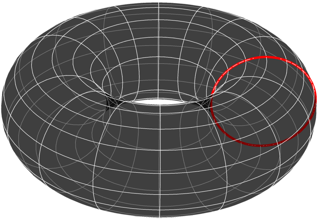
Figure 1: Pinching a torus: the red circle on the torus collapses to zero.

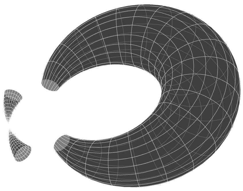
Figure 2: A cut of the pinched torus. The component on the right is Riemannian.

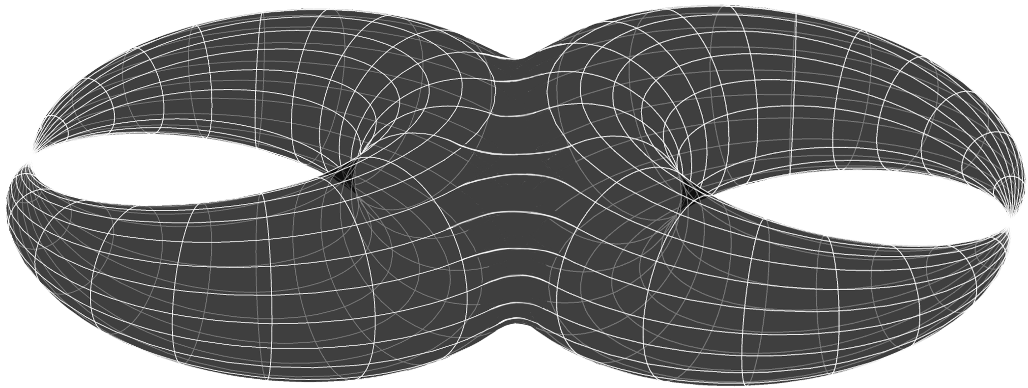
+     +     + $\cdots$

Figure 3: Sum over the topologies of nodal Riemann spheres.

This is reminiscent of the situation of the one-loop ambitwistor string amplitude Geyer:2015bja , where the one-loop moduli space is localized to a discrete set of points selected by the scattering equations that encode the kinematics of particle scatterings. Using the “global residue theorem,” the contour integrals around these discrete points can be rewritten as the contour integral over the boundary of the fundamental domain for the torus moduli space, and the only nontrivial contribution comes from $\tau\rightarrow i\,\infty$ as in Eq. (53). This implies that we encounter the same worldsheet topology in the M0T string and ambitwistor string theory, which is not a coincidence: as we will see in the next section, M0T is related to a corner that is connected to ambitwistor string theory via a timelike T-duality transformation.

It is interesting to note that the nodal Riemann sphere is almost a Riemann sphere: if we perform a cut of the worldsheet as in Fig. 2, then the component on the right is a regular Riemann surface. This suggests that it might be possible to map the string sigma model defined on this patch of the surface to be a conventional conformal field theory.

$\bullet$ Higher loop orders. The topology in the genus-$n$ case follows directly from our discussion on the genus-one case above: we just obtain a nodal Riemann sphere with $n$ pairs of identified points in the $\omega\rightarrow\infty$ limit from pinching different cycles on the genus-$n$ Riemann surface. Therefore, the path integral for the M0T string is associated with the sum of different topologies described by nodal Riemann surfaces as in Fig. 3. The Euler characteristics of the $n$-loop string worldsheet is given by

$$\chi_{\text{\scalebox{0.8}{E}}}=2-2\,n+\text{number of pinches}=2-n\,,$$ (54)

where the number of pinches is equal to the order of string loops. In the case of ambitwistor string theory, the number of the pairs of identified points on the Riemann sphere corresponds to the loop order of the associated Feynman diagrams Geyer:2015bja ; Geyer:2018xwu .

Later in Sections 3 and 4, we will build a duality web of string sigma models by performing T-duality transformations of the M0T string action. It is important to note that such perturbative duality transformations do not alter the nature of the worldsheet structure and the discussions of the worldsheet properties in this section continue to apply.

2.5 Worldsheet Symmetries and Gauge Fixing

We now study the symmetries of the M0T string action (41), with the focus on the worldsheet symmetries and the relevant gauge fixing. It is sufficient to consider the flat target space and the gauge fixing in the Carrollian parametrization of the worldsheet. This subsection essentially extends the findings in the previous work on non-vibrating strings Batlle:2016iel to the Polyakov formulation. See related discussions for the same worldsheet structure in the context of tensionless/ambitwistor string theory Isberg:1993av ; Bagchi:2013bga ; Casali:2016atr ; Chen:2023esw , Spin Matrix theory Harmark:2018cdl ; Harmark:2019upf ; Bidussi:2023rfs , and tropological sigma models Albrychiewicz:2023ngk . We will visit the connections udlstmt between M0T and these corners using T-duality later in this paper.

In the flat target space with $\tau_{\mu}{}^{0}=\delta_{\mu}^{0}$ , $E_{\mu}{}^{A^{\prime}}=\delta_{\mu}^{A^{\prime}}$ , and $B_{\mu\nu}=0$ , the M0T string action (41) becomes

$$S_{\text{M0T}}=\frac{T}{2}\int d^{2}\sigma\,e\,\biggl{[}\Bigl{(}e^{\alpha}_{1}\,\partial_{\alpha}X^{0}\Bigr{)}^{2}+e^{\alpha}_{0}\,e^{\beta}_{0}\,\partial_{\alpha}X^{A^{\prime}}\,\partial_{\beta}X^{A^{\prime}}+\lambda\,e^{\alpha}_{0}\,\partial_{\alpha}X^{0}\biggr{]}\,.$$ (55)

Under the reparametrization symmetry of the worldsheet coordinates $\sigma^{\alpha}\rightarrow\sigma^{\prime\alpha}(\tau,\sigma)$ , we have the following induced transformations on the zweibein fields $e_{\alpha}{}^{a}$ and the worldsheet fields $X^{\mu}$ and $\lambda$ :

$$e^{\prime}_{\alpha}{}^{a}(\tau^{\prime}\!,\sigma^{\prime})=\frac{\partial\sigma^{\beta}(\sigma)}{\partial\sigma^{\prime}{}^{\alpha}}\,e_{\beta}{}^{a}(\tau,\sigma)\,,\qquad X^{\prime}{}^{\mu}(\sigma^{\prime})=X^{\mu}(\sigma)\,,\qquad\lambda^{\prime}(\sigma^{\prime})=\lambda(\sigma)\,.$$ (56)

In addition, the action is invariant under the local worldsheet gauge symmetries

$$e^{0} \rightarrow h(\tau,\sigma)\,e^{0}+b(\tau,\sigma)\,e^{1}\,, X^{\mu} \rightarrow X^{\mu}\,,$$ (57a)

$$e^{1} \rightarrow h(\tau,\sigma)\,e^{1}\,, \lambda \rightarrow\frac{\lambda}{h}+\frac{b}{h^{3}}\,\bigl{(}2\,h\,e^{\alpha}{}_{1}-b\,e^{\alpha}{}_{0}\bigr{)}\,\partial_{\alpha}X^{0}\,,$$ (57b)

where $b(\sigma)$ parametrizes the local Carrollian boost that generalizes Eq. (34)) to finite transformations and $h(\sigma)$ parametrizes the local Weyl symmetry.

$\bullet$ Gauge fixing. The infinitesimal version of Eqs. (56) and (57) are

$$\delta e_{\alpha}{}^{0} =\xi^{\beta}\,\partial_{\beta}e_{\alpha}{}^{0}+e_{\beta}{}^{0}\,\partial_{\alpha}\xi^{\beta}+\theta\,e_{\alpha}{}^{0}+\beta\,e_{\alpha}{}^{1}\,,$$ (58a)

$$\delta e_{\alpha}{}^{1} =\xi^{\beta}\,\partial_{\beta}e_{\alpha}{}^{1}+e_{\beta}{}^{1}\,\partial_{\alpha}\xi^{\beta}+\theta\,e_{\alpha}{}^{1}\,,$$ (58b)

$$\delta X^{\mu} =\xi^{\alpha}\,\partial_{\alpha}X^{\mu}\,,$$ (58c)

$$\delta\lambda =\xi^{\alpha}\partial_{\alpha}\lambda-\theta\,\lambda+2\,\beta\,e^{\alpha}{}_{1}\,\partial_{\alpha}X^{0}\,.$$ (58d)

where $\xi^{\alpha}$ parametrizes the diffeomorphisms, $\theta$ the dilatation, and $\beta$ the worldsheet Carrollian boost. We choose the flat gauge $e_{\alpha}{}^{a}=\delta_{\alpha}^{a}$ , which implies $\delta e_{\alpha}{}^{a}=0$ . From Eqs. (58a) and (58b), we find

$$\theta=-\partial_{\tau}\xi^{\tau}=-\partial_{\sigma}\xi^{\sigma}\,,\qquad\beta=-\partial_{\sigma}\xi^{\tau}\,,\qquad\partial_{\tau}\xi^{\sigma}=0\,,$$ (59)

which are solved by

$$\xi^{\tau}=u^{\prime}(\sigma)\,\tau+v(\sigma)\,,\qquad\xi^{\sigma}=u(\sigma)\,,\qquad\theta=-u^{\prime}(\sigma)\,,\qquad\beta=-u^{\prime\prime}(\sigma)\,\tau-v^{\prime}(\sigma)\,.$$ (60)

From Eqs. (58c) and (58d), we find

$$\delta X^{\mu} =\bigl{(}u^{\prime}\,\tau+v\bigr{)}\,\partial_{\tau}X^{\mu}+u\,\partial_{\sigma}X^{\mu}\,,$$ (61a)

$$\delta\lambda =\bigl{(}u^{\prime}\,\tau+v\bigr{)}\,\partial_{\tau}\lambda+\bigl{(}u\,\lambda\bigr{)}^{\prime}-2\,\bigl{(}u^{\prime\prime}\,\tau+v^{\prime}\bigr{)}\,\partial_{\sigma}X^{0}\,.$$ (61b)

In this flat gauge, the M0T action (55) becomes

$$S_{\text{P}}=\frac{T}{2}\int d^{2}\sigma\,\Bigl{(}\partial_{\sigma}X^{0}\,\partial_{\sigma}X^{0}+\partial_{\tau}X^{A^{\prime}}\partial_{\tau}X^{A^{\prime}}+\lambda\,\partial_{\tau}X^{0}\Bigr{)}\,,$$ (62)

We recalled that the target space symmetry is now nonrelativistice, as the M0T string action (55) is invariant under the global transformations

$$X^{0}\rightarrow\Xi^{0}\,,\qquad X^{A^{\prime}}\rightarrow\Xi^{A^{\prime}}+\Lambda^{A^{\prime}}\,X^{0}\,,\qquad\lambda\rightarrow\lambda-2\,\Lambda_{A^{\prime}}\,\partial_{\tau}X^{A^{\prime}}\,.$$ (63)

Here, $\Lambda^{A^{\prime}}$ is associated with the target space Galilean boost (8) (and Eq. (42)). The target space Lorentz symmetry in conventional string theory is, however, broken now.

Following the reparametrizations of the target space data in Eq. (12) and of the worldsheet metric in Eq. (33), the critical RR 1-form limit of type IIA superstring theory is now rephrased as a rescaling of both the worldsheet and spacetime coordinates in the flat case: 

$$X^{0}\rightarrow\omega^{1/2}\,X^{0}\,,\qquad X^{A^{\prime}}\rightarrow\omega^{-1/2}\,X^{A^{\prime}}\,,\qquad\tau\rightarrow\omega^{-1}\,\tau\,,\qquad\sigma\rightarrow\sigma\,,$$ (64)

Plugging Eq. (64) into the conventional string sigma model

$$\hat{S}_{\text{P}}=-\frac{T}{2}\int d^{2}\sigma\,\partial_{\alpha}X^{\mu}\,\partial^{\alpha}X_{\mu}\,,$$ (65)

we find

$$\hat{S}_{\text{P}}\rightarrow\frac{T}{2}\int d^{2}\sigma\,\Bigl{[}-\omega^{2}\,\bigl{(}\partial_{\tau}X^{0}\bigr{)}^{2}+\partial_{\sigma}X^{0}\,\partial_{\sigma}X^{0}+\partial_{\tau}X^{A^{\prime}}\partial_{\tau}X^{A^{\prime}}+O\bigl{(}\omega^{-2}\bigr{)}\Bigr{]}\,.$$ (66)

Using the Hubbard-Stratonovich transformation to integrate in an auxiliary field $\lambda$ as in Eq. (44) followed by taking the infinte $\omega$ limit, we recover the M0T string action (62).

$\bullet$ Tropological sigma models. Intriguingly, if $X^{2}=\cdots X^{9}=0$ , the M0T string action (62) can be identified with the bosonic part of tropological sigma models recently proposed in Albrychiewicz:2023ngk . More specifically, identify $T=e^{-1}$ , $\tau=\theta$ , $\sigma=r$ , $\lambda=2\,\bigl{(}\beta-\partial_{r}\Theta\bigr{)}$ , $X^{0}=X$ , and $X^{1}=\Theta$ in the M0T string action (62), we find 

$$S=\frac{1}{e}\int dr\,d\theta\,\Bigl{[}\tfrac{1}{2}\bigl{(}\partial_{\theta}\Theta-\partial_{r}X\bigr{)}^{2}+\beta\,\partial_{\theta}X+\text{total derivative}\Bigr{]}\,.$$ (67)

Up to a boundary term, Eq. (67) is identical to the bosonic part of the tropological sigma model (3.21) in Albrychiewicz:2023ngk . Such tropological sigma model is partly motivated by the study of Gromov-Witten invariants in topological QFTs, as some of these invariants can be computed by performing the “tropical” limit of the associated geometries. In the target space, the tropological sigma model realizes the geometric structures associated with tropical localization equations, while the tropicalization of the worldsheet metric essentially gives the Carrollian worldsheet that we have discussed around Eq. (33). The tropical geometry is a useful mathematical concept that naturally appears in a range of different fields including computer science, e.g. the Floyd-Warshall algorithm, which is a dynamic-programming method that solves the all-pairs shortest-paths problem on a directed graph cormen2022introduction . It is argued in Albrychiewicz:2023ngk that the nonrelativistic worldsheet of the tropological sigma models shares similarities with the worldsheet of nonequilibrium string perturbation theory, i.e. the string theoretical version of the Schwinger-Keldysh formalism Horava:2020she ; Horava:2020val ; Horava:2020apz .

$\bullet$ Galilean conformal algebra. There is a residual gauge symmetry, i.e. a reparametrization of the worldsheet coordinates, that leaves the M0T string action (62) invariant. We start with a general reparametrization of the worldsheet coordinates with $\tau\rightarrow T(\tau,\sigma)$ and $\sigma\rightarrow\Sigma(\tau,\sigma)$ , together with $\lambda\rightarrow\lambda+\Delta(\tau,\sigma)$ . Requiring that the action (62) be invariant implies

$$\partial_{\tau}\Sigma=0\,,\qquad\partial_{\tau}T=\partial_{\sigma}\Sigma\,,\qquad\Delta=\frac{1}{\partial_{\sigma}\Sigma}\left[\lambda+2\,\partial_{\sigma}X^{0}\,\frac{\partial_{\sigma}T}{\partial_{\sigma}\Sigma}-\partial_{\tau}X^{0}\left(\frac{\partial_{\sigma}T}{\partial_{\sigma}\Sigma}\right)^{2}\right].$$ (68)

Therefore, the residual worldsheet diffeomorphisms are

$$\tau\rightarrow T(\tau,\sigma)=\mathcal{S}^{\prime}(\sigma)\,\tau+\mathcal{T}(\sigma)\,.\qquad\sigma\rightarrow\Sigma(\tau,\sigma)=\mathcal{S}(\sigma)\,,$$ (69)

for arbitrary functions $\mathcal{S}$ and $\mathcal{T}$ of the worldsheet spatial coordinate $\sigma$ . Note that these transformations are accompanied with an appropriate reparametrization $\lambda\rightarrow\lambda+\Delta$ of the Lagrange multiplier $\lambda$ , where $\Delta$ is given in Eq. (68).

In the infinitesimal case, we write

$$\delta\tau=\xi^{\prime}(\sigma)\,\tau+\zeta(\sigma)\,,\qquad\delta\sigma=\xi(\sigma)\,.$$ (70)

These transformations are generated by the operators

$$L=\xi^{\prime}(\sigma)\,\tau\,\partial_{\tau}+\xi(\sigma)\,\partial_{\sigma}\,,\qquad M=\zeta(\sigma)\,\partial_{\tau}\,.$$ (71)

The Fourier expansions $\xi=\sum_{n}k_{n}\,e^{i\,n\,\sigma}$ and $\zeta=\sum_{n}z_{n}\,e^{i\,n\,\sigma}$ imply $L=i\sum_{n}k_{n}\,L_{n}$ and $M=i\sum_{n}z_{n}\,M_{n}$, with

$$L_{n}=e^{i\,n\,\sigma}\,\bigl{(}-n\,\tau\,\partial_{\tau}+i\,\partial_{\sigma}\bigr{)}\,,\qquad M_{n}=i\,e^{i\,n\,\sigma}\,\partial_{\tau}\,.$$ (72)

These generators form the two-dimensional worldsheet Galilean conformal algebra Bagchi:2009pe ; Bagchi:2009my ; Bagchi:2013bga ,

$$\bigl{[}L_{n}\,,L_{m}\bigr{]}=\bigl{(}n-m\bigr{)}\,L_{n+m}\,,\qquad\bigl{[}L_{n}\,,M_{m}\bigr{]}=\bigl{(}n-m\bigr{)}\,M_{n+m}\,,\qquad\bigl{[}M_{n}\,,M_{m}\bigr{]}=0\,,$$ (73)

which is isomorphic to the Bondi-Metzner-Sachs (BMS) algebra Bondi:1962px ; Sachs:1962zza in three dimensions Bagchi:2010zz . At the classical level, there is no central extension. See Bagchi:2009pe for central extensions of the Galilean conformal algebra.

$\bullet$ Equations of motion. The equations of motion from varying the worldsheet fields in the gauge-fixed action (62) are

$$\partial_{\tau}X^{0}=\partial_{\tau}\lambda+2\,\partial_{\sigma}^{2}X^{0}=\partial_{\tau}^{2}X^{A^{\prime}}=0\,,$$ (74)

which are solved by

$$X^{0}\bigl{(}\tau,\sigma\bigr{)} =f_{1}\bigl{(}\sigma\bigr{)}\,,\qquad\lambda\bigl{(}\tau,\sigma\bigr{)}=f_{2}\bigl{(}\sigma\bigr{)}-2\,f^{\prime\prime}_{1}\bigl{(}\sigma\bigr{)}\,\tau\,,$$ (75a)

$$X^{A^{\prime}}\!\bigl{(}\tau,\sigma\bigr{)} =g_{1}^{A^{\prime}}\!(\sigma)+g_{2}^{A^{\prime}}\!(\sigma)\,\tau\,.$$ (75b)

Because the embedding coordinates do not satisfy any wave function, the M0T string is called non-vibrating string in Batlle:2016iel . This non-vibrating feature is ubiquitous for different fundamental strings related to the M0T string via T-duality. Under the residual worldsheet gauge transformation of $X^{\mu}$ in Eq. (61), we find that $f_{1}$ , $g_{1}^{A^{\prime}}$, and $g_{2}^{A^{\prime}}$ transform as

$$\delta f_{1}=u\,f^{\prime}_{1}\,,\qquad\delta g_{1}^{A^{\prime}}=u\,\bigl{(}g_{1}^{A^{\prime}}\bigr{)}^{\prime}+v\,g_{2}^{A^{\prime}}\,,\qquad\delta g_{2}^{A^{\prime}}=\bigl{(}u\,g_{2}^{A^{\prime}}\bigr{)}^{\prime}\,.$$ (76)

Furthermore, the residual gauge transformation (61b) of $\lambda$ implies

$$\delta f^{\prime\prime}_{1}=\bigl{(}u\,f^{\prime}_{1}\bigr{)}^{\prime\prime}\,,\qquad\delta f_{2}=\bigl{(}u\,f_{2}\bigr{)}^{\prime}-2\,\bigl{(}v\,f_{1}^{\prime}\bigr{)}^{\prime}\,.$$ (77)

It is reassuring to observe that the transformations $\delta f_{1}$ in Eq. (76) and $\delta f^{\prime\prime}_{1}$ in Eq. (77) match each other, which ensures that $u=u(\sigma)$ is not constrained. We can therefore use $u(\sigma)$ to gauge fix $f_{1}(\sigma)$ to be $\sigma$ and use $v(\sigma)$ to gauge fix $f_{2}(\sigma)$ to a constant, i.e.,

$$X^{0}\!=\sigma\,,\qquad X^{A^{\prime}}\!\!=x^{A^{\prime}}(\sigma)+T^{-1}P^{A^{\prime}}(\sigma)\,\tau\,,\qquad\lambda=2\,T^{-1}P_{0}\,,$$ (78)

where $P_{0}$ is the conjugate momentum of $X^{0}$ and $P_{A^{\prime}}(\sigma)$ the conjugate momentum of $X^{A^{\prime}}$. The constant $P_{0}$ represents the constant effective energy of the string. Using the Hamiltonian constraints imposed by $\chi$ and $\rho$ , respectively, in the phase space action (21), we find

$$P_{A^{\prime}}(\sigma)\,P^{A^{\prime}}\!(\sigma)=T^{2},\qquad P_{0}=-P_{A^{\prime}}(\sigma)\,\frac{dx^{A^{\prime}}\!(\sigma)}{d\sigma}\,.$$ (79)

The following Virasoro-like constraints arise from varying the worldsheet zweibein fields $e_{\alpha}{}^{a}$ in Eq. (55) and then fixing the gauge:

$$-\bigl{(}\partial_{\sigma}X^{0}\bigr{)}^{2}+\partial_{\tau}X^{A^{\prime}}\,\partial_{\tau}X^{A^{\prime}} =0\,, \lambda\,\partial_{\tau}X^{0} =0\,,$$ (80a)

$$\partial_{\sigma}X^{0}\,\partial_{\tau}X^{0} =0\,, \lambda\,\partial_{\sigma}X^{0}+2\,\partial_{\tau}X^{A^{\prime}}\,\partial_{\sigma}X^{A^{\prime}} =0\,.$$ (80b)

These equations are consistent (by definition) with the solutions in Eqs. (79) and (78).

$\bullet$ Massless Galilean system and geometric optics. We now focus on the string state with a constant collective momentum, i.e. we only keep the zero mode in $P_{A^{\prime}}(\sigma)$ . For this purpose, we treat $P_{A^{\prime}}$ as a constant. As $P_{0}$ is also a constant, the second Hamiltonian constraint in Eq. (79) implies that

$$x^{A^{\prime}}=X^{A^{\prime}}_{0}+V^{A^{\prime}}X^{0}\,,$$ (81)

where $X^{A^{\prime}}_{0}$ marks the position of the string and $V^{A^{\prime}}$ is the center-of-mass velocity of the string in the target space. From Eq. (79), we find the dispersion relation,

$$P_{A^{\prime}}P^{A^{\prime}}=T^{2}\,,\qquad P_{0}=-V^{A^{\prime}}P_{A^{\prime}}\,.$$ (82)

In order to understand the physics of the zero mode derived in Eq. (82), we first consider the spacetime Galilean boost that acts nontrivially on $x^{A^{\prime}}$ and $P_{0}$ as

$$\delta_{\text{G}}x^{A^{\prime}}=v^{A^{\prime}}X^{0}\,,\qquad\delta_{\text{G}}P_{0}=-v^{A^{\prime}}P_{A^{\prime}}\,.$$ (83)

The solution (79) to the Hamiltonian constraints are clearly invariant under the Galilean boost (83). Eq. (81) implies that the Galilean boost (83) acts on $V^{A^{\prime}}$ as $\delta V^{A^{\prime}}=-v^{A^{\prime}}$. Therefore, we can always perform a Galilean boost to go to the “rest frame” with $V^{A^{\prime}}=0$ , such that the dispersion relation (82) becomes

$$\text{\emph{rest frame:}}\qquad P_{A^{\prime}}\,P^{A^{\prime}}\!=T^{2}\,,\qquad P_{0}=0\,.$$ (84)

Since the excitation has zero energy in the rest frame, it behaves like a phonon but with Galilean symmetry. However, the spatial momentum of the excitation always has a fixed length. This is a massless Galilean system, which can be obtained from a Galilean limit of the Souriau tachyon, where the mass is imaginary Batlle:2017cfa ; souriau1970structure .

The seemingly exotic dispersion relation (84) of the massless Galilean system in fact describes the ordinary physics of geometric optics Duval:2005ry ; Duval:2013aza . Define the optical length from point $p_{1}$ to point $p_{2}$ via a spatial path $X^{A^{\prime}}(s)$ to be

$$S=\int_{p_{1}}^{p_{2}}ds\,n\bigl{(}x^{A^{\prime}}\bigr{)}\,,$$ (85)

where $n=n(x^{A^{\prime}})$ is the index of refraction and $ds=\sqrt{dx^{A^{\prime}}\,dx^{A^{\prime}}}$ is the element of arc length. Fermat’s principle states that the physical light ray is selected by minimizing the action (85). The conjugate momentum with respect to $x^{A^{\prime}}$ is

$$P_{A^{\prime}}=n\,\frac{dx^{A^{\prime}}}{ds}\,,$$ (86)

which implies the dispersion relation $P_{A^{\prime}}\,P^{A^{\prime}}=n^{2}$ . Moreover, the associated Hamiltonian vanishes, i.e. $P_{0}=0$ . This precisely matches Eq. (84) after identifying the index of refraction $n$ with the string tension $T$ .

3 The First DLCQ: Spacelike and Timelike T-Dualities

In this section we classify spacelike and timelike T-duality transformations starting with the string action (41) in Matrix 0-brane Theory (M0T), which arises from the critical RR 1-form limit of the conventional string action. Studying these T-duality transformations will allow us to build a zoo of decoupling limits of type II (and type II^∗ Hull:1998vg ) string theories connected to a single DLCQ of M-theory. Later in Section 4 we will discuss how a second DLCQ of M-theory can be implemented, which leads to another layer of duality web udlstmt . For pedagogical reason, we always start with focusing on flat spacetime and then discuss the curved spacetime generalization later in each subsection.

3.1 Spacelike T-Duality: Strings in Matrix $p$-Brane Theory

We start with the discussions on spacelike T-duality transformations of the M0T string, which will lead us to the fundamental strings in general Matrix $p$-brane theories (M$p$Ts) with $p\geq 0$ . The light excitations in M$p$T are the D$p$-branes, which are described by the associated Matrix gauge theory udlstmt .

3.1.1 Strings in Flat Spacetime

The flat-spacetime M0T string action has been given in Eq. (62). We start with compactifying the spatial directions $X^{u}$, $u=1\,,\cdots\,,p$ over circles of radii $R_{1}\,,\cdots,R_{p}$ , respectively, and perform a T-duality transformation along each of these circles. This can be done by gauging the isometries $X^{u}$ and rewrite Eq. (62) as

$$\begin{split}S_{\text{gauged}}=\frac{T}{2}\int d^{2}\sigma\,\Bigl{(}\partial_{\sigma}X^{0}\,\partial_{\sigma}X^{0}&+\partial_{\tau}X^{\widetilde{A}^{\prime}}\,\partial_{\tau}X_{\widetilde{A}^{\prime}}+\lambda\,\partial_{\tau}X^{0}\\[4.0pt] &+D_{\tau}X^{u}\,D_{\tau}X_{u}-2\,\epsilon^{\alpha\beta}\,\widetilde{X}_{u}\,\partial_{\alpha}v^{u}_{\beta}\Bigr{)}\,.\end{split}$$ (87)

where $\widetilde{A}^{\prime}=p+1\,,\cdots\,,9$ and $D_{\alpha}X^{u}=\partial_{\alpha}X^{u}+v^{u}_{\alpha}$ . This action preserves the U$(1)$ gauge symmetry $\delta X^{u}=-\xi^{u}$ and $\delta v^{u}_{\alpha}=\partial_{\alpha}\xi^{u}$ . The to-be dual coordinates $\widetilde{X}^{u}$ are Lagrange multipliers imposeing the that $v^{u}_{\alpha}$ is pure gauge. Integrating out $\widetilde{X}^{u}$ in Eq. (87) sets $\epsilon^{\alpha\beta}\,\partial_{\alpha}v^{u}_{\beta}=0$ , which can be solved locally by $v^{u}_{\alpha}=\partial_{\alpha}\Phi^{u}$ and it implies $D_{\alpha}X^{u}=\partial_{\alpha}(X^{u}+\Phi^{u})$ . After absorbing $\Phi^{u}$ into the definition of $X^{u}$, we recover the original action (62). Instead of integrating out $\widetilde{X}_{u}$ , integrating out $v^{u}_{\tau}$ in Eq. (87) gives the dual action,

$$\begin{split}\widetilde{S}_{\text{P}}&=-\frac{T}{2}\int d^{2}\sigma\,\biggl{[}\Bigl{(}-\partial_{\sigma}X^{0}\,\partial_{\sigma}X^{0}+\partial_{\sigma}\widetilde{X}^{u}\,\partial_{\sigma}\widetilde{X}_{u}\Bigr{)}-\partial_{\tau}X^{\widetilde{A}^{\prime}}\,\partial_{\tau}X_{\widetilde{A}^{\prime}}\\ &\hskip 97.30836pt-\Bigl{(}\lambda\,\partial_{\tau}X^{0}+2\,v^{u}_{\sigma}\,\partial_{\tau}\widetilde{X}_{u}\Bigr{)}-2\,\partial_{\tau}X^{u}\,\partial_{\sigma}\widetilde{X}_{u}\biggr{]}\,,\end{split}$$ (88)

where $v_{\sigma}^{u}$ stays as a Lagrange multiplier that imposes the constraint $\partial_{\tau}\widetilde{X}_{u}=0$ . Define $\lambda_{0}=\lambda$ and $\lambda_{u}=2\,D_{\!\sigma}X^{u}$ and drop the tilde in $\widetilde{X}^{u}$ and $X^{\widetilde{A}^{\prime}}$​, we find

$$\widetilde{S}_{\text{M$p$T}} =-\frac{T}{2}\int d^{2}\sigma\,\Bigl{(}\partial_{\sigma}X^{A}\,\partial_{\sigma}X_{A}-\partial_{\tau}X^{A^{\prime}}\partial_{\tau}X_{A^{\prime}}-\lambda_{A}\,\partial_{\tau}X^{A}\biggr{)}\,,$$ (89)

where we have ignored the topological term $\int dX^{u}\wedge d\widetilde{X}^{u}$ that encodes the winding Wilson lines Alvarez:1996up . Throughout the rest of the paper we will always ignore this topological term for simplicity. Here, $A=0\,,\cdots,\,p$ and $A^{\prime}=p+1\,,\cdots,9$ . The dual action (89) arises from the critical RR $(p+1)$-form limit of the conventional string sigma model (65). This critical limit is prescribed by the coordinate rescalings,

$$X^{A}\rightarrow\omega^{1/2}\,X^{A}\,,\qquad X^{A^{\prime}}\rightarrow\omega^{-1/2}\,X^{A^{\prime}}\,,\qquad\tau\rightarrow\omega^{-1}\,\tau\,,\qquad\sigma\rightarrow\sigma\,.$$ (90)

which provides the $p$-brane generalization of the rescaling (64). Plugging Eq. (90) into the conventional string action (65) followed by sending $\omega$ to infinity reproduces Eq. (89). The action (89) describes the fundamental string in the spacetime with a codimension-$(p+1)$ foliation structure, which admits a spacetime $p$-brane Galilean boost,

$$\delta_{p\text{G}}X^{A}=0\,,\qquad\delta_{p\text{G}}X^{A^{\prime}}=\Lambda_{A}{}^{A^{\prime}}\,X^{A},\qquad\delta_{p\text{G}}\lambda_{A}=-2\,\Lambda_{AA^{\prime}}\,\partial_{\tau}X^{A^{\prime}}.$$ (91)

This $p$-brane Galilean boost naturally generalizes the particle case in Eq. (8).

The prescriptions in Eq. (90) define a critical RR ($p$+1)-form limit of type II string theory. The reason why a critical RR ($p$+1)-form is required for this limit to work is the following: a critical RR 1-form in (12) is required in the M0T limit Gopakumar:2000ep . Under T-dualities, this critical RR 1-form is eventually dualized to be the critical RR ($p$+1)-form. This corner of type II string theory that arises from such the critical RR ($p$+1)-form limit is referred to as Matrix $p$-brane Theory (M$p$T) udlstmt . This name is motivated by the fact that the critical RR $(p+1)$-form limit of a stack of D$p$-branes leads to Matrix gauge theory Obers:1998fb , i.e., Matrix theory compactified over a vanishing $p$-torus. For example, when $p=1$ , the Matrix gauge theory is Matrix string theory Dijkgraaf:1997vv . When $p=3$, the Matrix gauge theory is $\mathcal{N}=4$ SYM. See further details in udlstmt ; longpaper . Here, we content ourselves with performing the M$p$T limit of a single D$p$-brane, from which we will be able to provide a qualitative understanding of why the RR potential is required to be critical Gomis:2000bd ; Gomis:2005bj (see also Kamimura:2005rz for dual D-branes in this context). We start with the D$p$-brane action in conventional type II superstring theories, focusing on the bosonic part in flat target spacetime but with a nontrivial RR ($p+1$)-form background,

$$\hat{S}_{\text{D}p}=-T_{p}\int d^{p+1}\sigma\,e^{-\hat{\Phi}}\,\sqrt{-\det\Bigl{(}\partial_{\alpha}X^{\mu}_{\phantom{\dagger}}\,\partial_{\beta}X_{\mu}+F_{\alpha\beta}\Bigr{)}}+T_{p}\int\hat{C}^{(p+1)}\,.$$ (92)

Here, $F=dA$ is $U(1)$ gauge field strength on the brane. We have set all the other RR potentials except $\hat{C}^{(p+1)}$ to zero. Under the rescalings $X^{A}\rightarrow\omega^{1/2}X^{A}$ and $X^{A^{\prime}}\rightarrow\omega^{-1/2}X^{A^{\prime}}$ from Eq. (90), in the static gauge with $X^{A}=\sigma^{A}$, $A=0\,,\cdots,\,p$ , we find

$$\sqrt{-\det\Bigl{(}\partial_{\alpha}X^{\mu}_{\phantom{\dagger}}\,\partial_{\beta}X_{\mu}+F_{\alpha\beta}\Bigr{)}}\rightarrow\omega^{\frac{p-3}{2}}\biggl{[}\,\omega^{2}+\tfrac{1}{2}\Bigl{(}\partial^{\alpha}X^{A^{\prime}}\,\partial_{\alpha}X_{A^{\prime}}+F^{\alpha\beta}\,F_{\alpha\beta}\Bigr{)}+O\bigl{(}\omega^{-2}\bigr{)}\biggr{]}\,.$$ (93)

Note that we have aligned the brane with the longitudinal sector by going to the static gauge. Under the additional prescriptions Gopakumar:2000ep ; udlstmt ,

$$\hat{\Phi}=\Phi+\tfrac{p-3}{2}\,\ln\omega\,,\qquad\hat{C}^{(p+1)}=-\omega^{2}\,e^{-\Phi}\,dX^{0}\wedge\cdots dX^{p}\,,$$ (94)

we find that the $\omega\rightarrow\infty$ limit of the redefined Eq. (92) gives rise to the following finite D$p$-brane action Ebert:2021mfu :

$$S_{\text{D}p}=-\frac{T_{p}}{2}\int d^{p+1}\sigma\,e^{-\Phi}\,\Bigl{(}\partial^{\alpha}X^{A^{\prime}}\,\partial_{\alpha}X_{A^{\prime}}+F^{\alpha\beta}\,F_{\alpha\beta}\Bigr{)}\,.$$ (95)

It is shown explicitly in udlstmt ; longpaper that the nonabelian version of Eq. (95) gives rise to Matrix gauge theory, i.e. BFSS Matrix theory compactified on a vanishing $p$-torus Fischler:1997kp .

Figure 4: T-duality relations between different M$p$Ts and the associated Matrix theories on the critical D$p$-branes. In M$p$T, the RR ($p+1$)-form is taken to be critical and the spacetime geometry develops a ($p+1$)-dimensional sector longitudinal to the background critical D$p$-brane and a ($9-p$)-dimensional sector transverse to the same background brane. These sectors are related via a $p$-brane Galilean boost.

3.1.2 Strings in Curved Spacetime

Performing T-duality transformations along spatial isometries in the M0T string action (41) in curved spacetime gives rise to the M$p$T string sigma model in general background fields,

$$S_{\text{M$p$T}}=\frac{T}{2}\int d^{2}\sigma\,e\,\Bigl{(}-e^{\alpha}_{1}\,e^{\beta}_{1}\,\tau_{\alpha\beta}+e^{\alpha}_{0}\,e^{\beta}_{0}\,E_{\alpha\beta}+\lambda_{A}\,e^{\alpha}_{0}\,\tau_{\alpha}{}^{A}\Bigr{)}-T\int B\,.$$ (96)

Here, $\tau_{\mu\nu}=\tau_{\mu}{}^{A}\,\tau_{\nu}{}^{B}\,\eta_{AB}$ with $A=0\,,\cdots,\,p$ and $E_{\mu\nu}=E_{\mu}{}{}^{A^{\prime}}E_{\mu}{}{}^{A^{\prime}}$ with $A^{\prime}=p+1\,,\cdots,9$ . The target space geometry has a codimension-$(p+1)$ foliation stucture and is referred to as the $p$-brane Newton-Cartan geometry, where the usual local Lorentz boost is now broken into the local $p$-brane Galilean boost, i.e. $\delta_{\text{G}}\tau^{A}=0$ and $\delta_{\text{G}}E^{A^{\prime}}=\Lambda_{A}{}^{A^{\prime}}\tau^{A}$. The action (96) generalizes Eq. (89) to curved background fields. In the special case with the indices $A=0$ and $A^{\prime}=1\,,\cdots,9$ , the M$p$T string action (96) reproduces the M$0$T string action (41).

$\bullet$ Longitudinal spatial T-duality. We now derive the Buscher rules for the T-duality transformation of the M$p$T string sigma model (96). We start with the T-duality transformation along a longitudinal isometry. Consider the Killing vector $k^{\mu}$ satisfying

$$k^{\mu}\,\tau_{\mu}{}^{u}=0\,,\,\,u=0\,,\cdots\,,\,p-1\,,\qquad k^{\mu}\,\tau_{\mu}{}^{p}\neq 0\,,\qquad k^{\mu}\,E_{\mu}{}^{A^{\prime}}=0\,.$$ (97)

In the coordinates $X^{\mu}=(y\,,X^{i})$ adapted to $k^{\mu}$, where $y$ is defined via $\partial_{y}=k^{\mu}\,\partial_{\mu}$ , Eq. (97) becomes

$$\tau_{y}{}^{u}=0\,,\qquad\tau_{y}{}^{p}\neq 0\,,\qquad E_{y}{}^{A^{\prime}}=0\,.$$ (98)

We perform the T-duality transformation by gauging the isometry $y$ as in Eq. (87) followed by integrating out the U(1) gauge potential. The T-dual action is

$$\widetilde{S}_{\text{M($p$\,-1)T}} =\frac{T}{2}\int\!\!d^{2}\sigma\,e\,\Bigl{(}-e^{\alpha}_{1}\,e^{\beta}_{1}\,\widetilde{\tau}_{\alpha\beta}+e^{\alpha}_{0}\,e^{\beta}_{0}\,\widetilde{E}_{\alpha\beta}+\lambda_{u}\,e^{\alpha}_{0}\,\tau_{\alpha}{}^{u}\Bigr{)}-T\int B\,,$$ (99)

where $\widetilde{\tau}_{\mu\nu}=\tau_{\mu}{}^{u}\,\tau_{\nu}{}^{v}\,\eta_{uv}$ with $u=0\,,\cdots,\,p-1$ and $\widetilde{E}_{\mu\nu}=\widetilde{E}_{\mu}{}^{u^{\prime}}\widetilde{E}_{\nu}{}^{u^{\prime}}$ with $u^{\prime}=p\,,\cdots,9$ . The action (99) describes the fundamental string in M($p$ -1)T. The Buscher rules for the vielbein and $B$-fields for this T-duality map from M$p$T to M($p$ -1)T are given by

$$\widetilde{E}_{yy}=\frac{1}{\tau_{yy}}\,,\qquad\widetilde{E}_{yi} =\frac{B_{yi}}{\tau_{yy}}\,,\qquad\widetilde{E}_{ij}=E_{ij}+\frac{B_{yi}\,B_{yj}}{\tau_{yy}}\,.$$ (100a)

$$\widetilde{B}_{yi} =\frac{\tau_{yi}}{\tau_{yy}}\,,\qquad\widetilde{B}_{ij}=B_{ij}+\frac{B_{yi}\,\tau_{yj}-B_{yj}\,\tau_{yi}}{\tau_{yy}}\,.$$ (100b)

Note that the dual isometry $\widetilde{y}$ satisfies

$$\widetilde{\tau}_{y}{}^{u}=0\,,\qquad\widetilde{E}_{y}{}^{p}=\frac{1}{\tau_{y}{}^{p}}\,,\qquad\widetilde{E}_{y}{}^{A^{\prime}}=0\,.$$ (101)

This implies that $\widetilde{y}$ is transverse now.

$\bullet$ Transverse T-duality. Next, we consider the T-duality transformation of the M$p$T string sigma model (96) along a transverse isometry $y$ that satisfy

$$\tau_{y}{}^{A^{\prime}}=0\,,\qquad E_{y}{}^{p+1}\neq 0\,,\qquad E_{y}{}^{u^{\prime}}=0\,,\,\,u^{\prime}=p+2\,,\cdots\,,9\,.$$ (102)

We have gone to the adapted coordinates $X^{\mu}=(y\,,X^{i})$ . The T-dual action is

$$\widetilde{S}_{\text{M($p$\,+1)T}} =\frac{T}{2}\int\!\!d^{2}\sigma\,e\,\Bigl{(}-e^{\alpha}_{1}\,e^{\beta}_{1}\,\widetilde{\tau}_{\alpha\beta}+e^{\alpha}_{0}\,e^{\beta}_{0}\,\widetilde{E}_{\alpha\beta}+\widetilde{\lambda}_{u}\,e^{\alpha}_{0}\,\widetilde{\tau}_{\alpha}{}^{u}\Bigr{)}-T\int\widetilde{B}\,.$$ (103)

where

$$\widetilde{\tau}_{\mu\nu} =\widetilde{\tau}_{\mu}{}^{u}\,\widetilde{\tau}_{\nu}{}^{v}\,\eta_{uv}\,,\qquad u=(A\,,\,p+1)\,,\qquad\widetilde{\tau}_{\mu}{}^{A}=\tau_{\mu}{}^{A}\,.$$ (104)

Here, $u=0\,,\cdots\,,\,p+1$ and $\widetilde{E}_{\mu\nu}=\widetilde{E}_{\mu}{}^{u^{\prime}}\,\widetilde{E}_{\nu}{}^{u^{\prime}}$ with $u^{\prime}=p+2\,,\cdots\,,9$ . The action (103) describes the fundamental string in M($p$ +1)T. The Buscher rules for the vielbein fields and $B$-fields associated with this T-duality map from M$p$T to M($p$ +1)T are given below:

$$\widetilde{\tau}_{y}{}^{p+1} =\frac{1}{E_{y}{}^{p+1}}\,, \widetilde{\tau}_{i}{}^{p+1} =\frac{B_{yi}}{E_{y}{}^{p+1}}\,, \widetilde{\tau}_{y}{}^{A} =\widetilde{E}_{y\mu}=0\,,$$ (105a)

$$\widetilde{E}_{ij} =E_{i}{}^{u^{\prime}}\,E_{j}{}^{u^{\prime}}\,, \widetilde{B}_{yi} =\frac{E_{yi}}{E_{yy}}\,, \widetilde{B}_{ij} =B_{ij}+\frac{B_{yi}\,E_{yj}-B_{yj}\,E_{yi}}{E_{yy}}\,.$$ (105b)

The dual isometry $\widetilde{y}$ satisfies

$$\widetilde{\tau}_{y}{}^{A}=0\,,\qquad\widetilde{\tau}_{y}{}^{p+1}\neq 0\,,\qquad\widetilde{E}_{y}{}^{u^{\prime}}=0\,,$$ (106)

i.e. $\widetilde{y}$ is now longitudinal. The longitudinal and transverse T-dual relations between different M$p$Ts are illustrated in Fig. 4.

3.1.3 General Critical Ramond-Ramond Limit

In Section 3.1.2 we have derived the M$p$T string sigma model (96) in the Polyakov action using T-duality transformations. The string worldsheet is nonrelativistic, with the topology that we have discussed in Section 2.4. We have stated in Section 3.1.1 that the M$p$T string sigma model arises from a limiting procedure with a critical RR ($p$ +1)-form in Eq. (94). Below we show explicitly how the the Polyakov and Nambu-Goto formulations of the M$p$T string sigma models arise from this limiting procedure.

Covariantizing the reparametrizations in Eqs. (90) and (94) gives the prescription in arbitrary background geometry, Kalb-Ramond, dilaton and RR field below Gopakumar:2000ep ; udlstmt :

$$\hat{G}_{\mu\nu} =\omega\,\tau_{\mu\nu}+\omega^{-1}\,E_{\mu\nu}\,, \hat{\Phi} =\Phi+\frac{p-3}{2}\,\ln\omega\,,$$ (107a)

$$\hat{C}^{(p+1)} =\omega^{2}\,e^{-\Phi}\,\tau^{0}\wedge\cdots\wedge\tau^{p}+C^{(p+1)}\,.$$ (107b)

Moreover, $\hat{C}^{(q)}=C^{(q)}$ for $q\neq p+1$ and $\hat{B}=B$ . When $p=0$ , Eq. (107) reduces to the M0T prescription (12). Recall that $\tau_{\mu\nu}=\tau_{\mu}{}^{A}\,\tau_{\nu}{}^{B}\,\eta_{AB}$ with $A=0\,,\cdots,\,p$ and $E_{\mu\nu}=E_{\mu}{}^{A^{\prime}}\,E_{\nu}{}^{A^{\prime}}$ with $A^{\prime}=p+1\,,\cdots,\,9$ . See Gopakumar:2000ep ; Harmark:2000ff ; Hyun:2000cw for the same decoupling limits in the presence of particular brane configurations and Gomis:2000bd ; Danielsson:2000gi for the closed string limits independence of the presence of branes.

$\bullet$ Polyakov action. Together with the reparametrization of the worldsheet metric (33), we find that the conventional Polyakov string action (26) with an extra $B$-field becomes

$$\hat{S}_{\text{P}}=-\frac{T}{2}\int d^{2}\sigma\,e\,\Bigl{[}-e^{\alpha}_{0}\,e^{\beta}_{0}\,\bigl{(}\omega^{2}\,\tau_{\alpha\beta}+E_{\alpha\beta}\bigr{)}+e^{\alpha}_{1}\,e^{\beta}_{1}\,\bigl{(}\tau_{\alpha\beta}+\omega^{-2}\,E_{\alpha\beta}\bigr{)}\Bigr{]}-T\int B\,.$$ (108)

We introduce the Lagrange multipliers $\lambda_{A}$ to rewrite (108) equivalently as

$$\hat{S}_{\text{P}}= -\frac{T}{2}\int d^{2}\sigma\,e\,\Bigl{(}-e^{\alpha}_{0}\,e^{\beta}_{0}\,E_{\alpha\beta}+e^{\alpha}_{1}\,e^{\beta}_{1}\,\tau_{\alpha\beta}+\lambda_{A}\,e^{\alpha}_{0}\,\tau_{\alpha}{}^{A}\Bigr{)}$$ (109)

$$-\frac{T}{2}\int d^{2}\sigma\,\biggl{[}\epsilon^{\alpha\beta}\,B_{\alpha\beta}+\omega^{-2}\,e\,\Bigl{(}e^{\alpha}_{1}\,e^{\beta}_{1}\,E_{\alpha\beta}+\tfrac{1}{4}\,\lambda_{A}\,\lambda^{A}\Bigr{)}\biggr{]}\,.$$

In the $\omega\rightarrow\infty$ limit, we recover the M$p$T string sigma model (96).

$\bullet$ Nambu-Goto action. Next, we apply the limiting prescription (107) to the conventional Nambu-Goto action (10a) to derive the analogous M$p$T Nambu-Goto action. We start with rewriting Eq. (10a) as

$$\hat{S}_{\text{NG}}=-\frac{T}{2}\int d^{2}\sigma\biggl{[}v-\frac{1}{v}\det\bigl{(}\hat{G}_{\alpha\beta}\bigr{)}+\epsilon^{\alpha\beta}\,B_{\alpha\beta}\biggr{]}\,.$$ (110)

Using Eq. (107), we find

$$\det\bigl{(}\hat{G}_{\alpha\beta}\bigr{)}=\omega^{2}\,\det\bigl{(}\tau_{\alpha\beta}\bigr{)}+\epsilon^{\alpha\beta}\,\epsilon^{\gamma\delta}\,\tau_{\alpha\gamma}\,E_{\beta\delta}+\omega^{-2}\,\det\bigl{(}E_{\alpha\beta}\bigr{)}\,,$$ (111)

where

$$\det\bigl{(}\tau_{\alpha\beta}\bigr{)}=\Bigl{(}\epsilon^{\alpha\beta}\,\tau_{\alpha}{}^{A}\,\tau_{\beta}{}^{B}\Bigr{)}\,\Bigl{(}\epsilon^{\gamma\delta}\,\tau_{\gamma}{}^{C}\,\tau_{\delta}{}^{D}\Bigr{)}\,\eta_{AC}\,\eta_{BD}\,.$$ (112)

Introducing the auxiliary antisymmetric tensor $\lambda_{AB}$ , we rewrite the action (110) as

$$\begin{split}\hat{S}_{\text{NG}}=-\frac{T}{2}\int d^{2}\sigma\biggl{[}v&-\frac{1}{v}\,\Bigl{(}\epsilon^{\alpha\beta}\,\epsilon^{\gamma\delta}\,\tau_{\alpha\gamma}\,E_{\beta\delta}+\omega^{-2}\,E\Bigr{)}\\[4.0pt] &+\epsilon^{\alpha\beta}\,\tau_{\alpha}{}^{A}\,\tau_{\beta}{}^{B}\,\lambda_{AB}+\frac{v}{4\,\omega^{2}}\,\lambda_{AB}\,\lambda^{AB}+\epsilon^{\alpha\beta}\,B_{\alpha\beta}\biggr{]}\,.\end{split}$$ (113)

In the $\omega\rightarrow\infty$ limit, we find the following finite action from Eq. (113):

$$S_{\text{NG}}=-\frac{T}{2}\int d^{2}\sigma\biggl{(}v-\frac{1}{v}\,\epsilon^{\alpha\beta}\,\epsilon^{\gamma\delta}\,\tau_{\alpha\gamma}\,E_{\beta\delta}+\epsilon^{\alpha\beta}\,\tau_{\alpha}{}^{A}\,\tau_{\beta}{}^{B}\,\lambda_{AB}+\epsilon^{\alpha\beta}\,B_{\alpha\beta}\biggr{)}\,.$$ (114)

Finally, integrate out $v$ gives

$$S_{\text{NG}}=-T\int d^{2}\sigma\,\Bigl{(}\sqrt{-\epsilon^{\alpha\beta}\,\epsilon^{\gamma\delta}\,\tau_{\alpha\gamma}\,E_{\beta\delta}}+\epsilon^{\alpha\beta}\,\tau_{\alpha}{}^{A}\,\tau_{\beta}{}^{B}\,\lambda_{AB}\Bigr{)}-T\int B\,.$$ (115)

When the longitudinal index $A$ is one-dimensional, the Lagrange multiplier term in Eq. (115) drops out and Eq. (115) coincides with the Nambu-Goto action (7) of the M0T string.

Now, we show that the Nambu-Goto action (115) is equivalent to the Polyakov action (96) of the M$p$T string. Note that the Lagrange multiplier $\lambda_{AB}$ in (115) imposes the constraint $\epsilon^{\alpha\beta}\,\tau_{\alpha}{}^{A}\,\tau_{\beta}{}^{B}=0$ , which is solved by $\tau_{\alpha}{}^{A}=\Gamma^{A}\,\tau_{\alpha}$ . Plugging this solution to $\tau_{\alpha}{}^{A}$ back into Eq. (115), we find

$$S_{\text{NG}}=-T\int d^{2}\sigma\,\sqrt{\Gamma^{\!A}\,\Gamma_{\!A}\,\det\!\begin{pmatrix}0&\,\,\tau_{\beta}\\[4.0pt] \tau_{\alpha}&\,\,E_{\alpha\beta}\end{pmatrix}}-T\int B\,.$$ (116)

On the other hand, starting with the Polyakov action (96) and integrate out the Lagrange multiplier $\lambda_{A}$ , we find the constraint $e^{\alpha}_{0}\,\tau_{\alpha}{}^{A}=0$ , which is solved by

$$e^{\alpha}_{0}=\epsilon^{\alpha\beta}\,\tau_{\beta}\,,\qquad\tau_{\alpha}{}^{A}=\Gamma^{A}\,\tau_{\alpha}\,.$$ (117)

Plugging Eq. (117) back into the Polyakov action (96) yields

$$S_{\text{M$p$T}}=\frac{T}{2}\int d^{2}\sigma\,\left[-\chi\,\Gamma^{A}\,\Gamma_{A}-\frac{1}{\chi}\det\!\begin{pmatrix}0&\,\,\tau_{\beta}\\[4.0pt] \tau_{\alpha}&\,\,E_{\alpha\beta}\end{pmatrix}\right],\qquad\chi=e^{\alpha}_{1}\,\tau_{\alpha}\,.$$ (118)

As expected, tntegrating out $\chi$ in Eq. (118) gives rise to Eq. (116).

3.2 Timelike T-Duality: Tensionless and Carrollian Strings

The second class of T-dualities that we consider here is the T-duality transformation along a target space timelike isometry in Matrix $p$-brane theory. T-duality in a timelike direction was first introduced in Hull:1998vg , where it is shown that type IIA (IIB) superstring theory maps to the IIB^∗ (IIA^∗) theory, which are different theories where certain background fields are essentially complexified. In such type II^∗ theories, the type II D-branes are mapped to Euclidean branes, which are localized in time and are also known as S(pacelike)-branes in Gutperle:2002ai . In the IIB^∗ theory, the spacelike D3-branes are argued to be holographically dual to de Sitter space Hull:1998vg ; Hull:2001ii . In this subsection, we will provide a worldsheet perspective for how this timelike T-duality relation between type II and type II^∗ theories works in the critical Ramond-Ramond field limits udlstmt . We will show how Matrix $p$-brane theories connect to tensionless, ambitwistor, and Carrollian string theories at the worldsheet level.

3.2.1 IKKT Matrix Theory and Tensionless String

Figure 5: A road map for the timelike T-dual relation between M$p$T and M(-$p$ -1)T and the spacelike T-duality relation between M$p$Ts with $p<0$.

$\bullet$ Flat spacetime. We start with considering the timelike T-duality transformation of the M0T string sigma model (62) in flat spacetime. For this purpose, we gauge the timelike isometry $X^{0}$ and rewrite Eq. (62) as

$$S_{\text{gauged}}=\frac{T}{2}\int d^{2}\sigma\,\Bigl{(}D_{\!\sigma}X^{0}\,D_{\!\sigma}X^{0} +\partial_{\tau}X^{A^{\prime}}\,\partial_{\tau}X_{A^{\prime}}+\lambda\,\partial_{\tau}X^{0}-2\,\widetilde{X}^{0}\,\epsilon^{\alpha\beta}\,\partial_{\alpha}v_{\beta}\Bigr{)}\,,$$ (119)

where $D_{\alpha}X^{0}=\partial_{\alpha}X^{0}+v_{\alpha}$ . The Lagrange multiplier $\widetilde{X}^{0}$ imposes the condition that $v_{\alpha}$ is pure gauge. The equations of motion from varying $v_{\alpha}$ are

$$\lambda=2\,\partial_{\sigma}\widetilde{X}^{0}\,,\qquad v_{\sigma}=-\partial_{\tau}\widetilde{X}^{0}-\partial_{\sigma}X^{0}\,.$$ (120)

Plugging Eq. (120) into the action (119), we find the dual action (up to a topological term associated with winding Wilson lines)

$$S_{\text{M(-1)T}}=\frac{T}{2}\int d^{2}\sigma\,\partial_{\tau}X^{\mu}\,\partial_{\tau}X_{\mu}\,.$$ (121)

This is the string sigma model in M(-1)T, where the target space geometry is Lorentzian. The action (121) can be thought of as the $p=-1$ extension of the M$p$T string sigma model (96).

$\bullet$ General backgrounds and type IIB^∗. The decoupling limit of string theory that leads to M(-1)T has been given in udlstmt , which we discuss below to be self-contained. Naïvely, one would expect that M(-1)T is a special case of M$p$T with $p=-1$ . A natural guess of how to extend the reparametrization (107) to $p=-1$ is

$$\hat{G}_{\mu\nu} =\omega^{-1}\,\tau_{\mu\nu}\,, \hat{\Phi} =\Phi-2\,\ln\omega\,,$$ (122a)

$$\hat{C}^{(0)} =\omega^{2}\,e^{-\Phi}+C^{(0)}\,, \hat{C}^{(q)} =C^{(q)}\,,\,\,q\neq 0\,, \hat{B} =B\,.$$ (122b)

Here, $\tau_{\mu\nu}=\tau_{\mu}{}^{A}\,\tau_{\nu}{}^{B}\,\eta_{AB}$ , $A=0\,,\,\cdots,9$ . Note that we stick to the notation where $\tau_{\mu\nu}$ (instead of $E_{\mu\nu}$) contains the time component. However, this naïve extrapolation is not quite right. The hidden subtlety already becomes manifest by e.g. applying Eq.(122) to a single D1-brane action in type IIB superstring theory,

$$\hat{S}_{\text{D$1$}}=-T_{1}\int d^{2}\sigma\,e^{-\hat{\Phi}}\,\sqrt{-\det\Bigl{(}\hat{G}_{\alpha\beta}+\hat{\mathcal{F}}_{\alpha\beta}\Bigr{)}}+T_{1}\int\Bigl{(}\hat{C}^{(2)}+\hat{C}^{(0)}\,\hat{\mathcal{F}}\Bigr{)}\,,$$ (123)

where $\hat{\mathcal{F}}=\hat{B}+F$ , with $F=dA$ the U(1) gauge field strength. Plugging Eq. (122) into the D1-brane action (123) leads to a leftover $\omega$ divergence,

$$\hat{S}_{\text{D1}}=\bigl{(}1+i\bigr{)}\,\omega^{2}\,e^{-\Phi}\,\mathcal{F}_{01}+O\bigl{(}\omega^{0}\bigl{)}\,.$$ (124)

We have chosen the branch with $\mathcal{F}_{01}<0$ , where $\mathcal{F}=B+F$ .  This divergence vanishes identically if one replaces in Eq. (122) either the $\hat{\Phi}$ prescription with

$$\hat{\Phi}=\Phi+\frac{i\pi}{2}-2\,\ln\omega$$ (125)

or the $\hat{C}^{(0)}$ prescription with $\hat{C}^{(0)}=i\,\omega^{2}\,e^{-\Phi}+C^{(0)}$ (but not both). The resulting theory is Euclidean NCYM on spacelike one-brane that is T-dual to 4D NCYM on D3-brane in M1T. This necessity of introducing an extra factor $i$ in the dilaton reparametrization can also be understood by using the standard Buscher rule for the dilaton transformation,

$$\widetilde{\Phi}=\Phi-\frac{1}{2}\ln k^{2}\,,$$ (126)

where $k_{\mu}$ is a timelike Killing vector, i.e. $k^{2}<0$ . Hence, with a specific choice of the branch,

$$\widetilde{\Phi}=\Phi+\frac{i\pi}{2}-\frac{1}{2}\ln|k^{2}|\,.$$ (127)

The appearance of the factor $i$ in the dilaton term is a general feature of timelike T-duality. In fact, the timelike T-duality maps type II superstring theories to the so-called type II^∗ theories, where the latters admit S(pacelike)-branes that are localized in time Hull:1998vg .

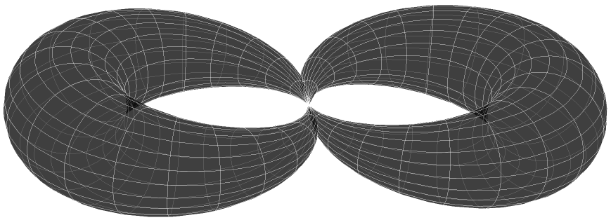
Figure 6: A more general Deligne-Mumford compactification of Riemann surface.

$\bullet$ IKKT Matrix theory. The dynamics of M(-1)T, which is of type IIB^∗ , is captured by the D(-1)-instantons from T-dualizing BFSS Matrix theory on the D0-branes in M0T along a timelike isometry. This procedure gives rise to Ishibashi-Kawai-Kitazawa-Tsuchiya (IKKT) Matrix theory on the D(-1)-instantons in M(-1)T Ishibashi:1996xs ,

$$S_{\text{IKKT}}=-\frac{1}{2\,g^{2}}\,\text{tr}\Bigl{(}\tfrac{1}{2}\,\bigl{[}A_{\mu}\,,A_{\nu}\bigr{]}^{2}+\bar{\Psi}\,\Gamma^{\mu}\bigl{[}A_{\mu}\,,\Psi\bigr{]}\Bigr{)}\,,$$ (128)

where the vector $A_{\mu}$ and the Majorana-Weyl spinor $\Psi$ are $N\times N$ matrices. Moreover, $\Gamma^{\mu}$ is the Weyl-projected $16\times 16$ Dirac matrices in ten dimensions. The IKKT Matrix theory was originally proposed as a nonperturbative regularization of the Green-Schwarz IIB superstring sigma model in the Schild formulation.

The string worldsheet topology in M(-1)T is the same as M0T that we have discussed in Section 2.4. They are nodal Riemann spheres. The existence of the pinching on the M$0$T string worldsheet might imply that the fundamental strings interact with each other via instantons at the pinching points. It is therefore suggestive to consider more general Deligne-Mumford compactifications of Riemann surfaces (see e.g. Fig. 6), and it would be interesting to see whether there is any connection to some version of string field theory that involves instantons. The conjectured string field-theoretical dynamics may be ultimately encoded by IKKT Matrix theory. Moreover, the brane objects other than the D-instanton in M(-1)T also acquire well-defined effective actions from taking the M(-1)T limit of conventional D$p$-brane actions using Eq. (122). See also Bagchi:2020ats for discussions on a D-instanton state in the context of tensionless string theory.

$\bullet$ Buscher rules for timelike T-duality. The M(-1)T string action (121) can be obtained from T-dualizing the M0T string sigma model (55) along a timelike isometry, which we demonstrate below. Start with the M0T string action (55) with a timelike isometry direction $y$ , which satisfies

$$\tau_{y}{}^{0}\neq 0\,,\qquad E_{y}{}^{A^{\prime}}=0\,.$$ (129)

T-dualizing $y$ gives rise to the dual action

$$\widetilde{S}_{\text{M(-1)T}}=\frac{T}{2}\int d^{2}\sigma\,e\,e^{\alpha}_{0}\,e^{\beta}_{0}\,\partial_{\alpha}X^{\mu}\,\partial_{\beta}X^{\nu}\,\widetilde{\tau}_{\mu\nu}-T\int\widetilde{B}\,,$$ (130)

with $\widetilde{\tau}_{\mu\nu}=\widetilde{\tau}_{\mu}{}^{A}\,\widetilde{\tau}_{\nu}{}^{B}\,\eta_{AB}$ , $A=0\,,\cdots,\,p$ and the Buscher rules from M0T to M(-1)T being akin to the ones in Eq. (100) from longitudinal spatial T-duality,

$$\widetilde{\tau}_{yy} =-\frac{1}{(\tau_{y}{}^{0})^{2}}\,, \widetilde{\tau}_{yi} =-\frac{B_{yi}}{(\tau_{y}{}^{0})^{2}}\,,\qquad\widetilde{\tau}_{ij}=E_{ij}-\frac{B_{yi}\,B_{yj}}{(\tau_{y}{}^{0})^{2}}\,.$$ (131a)

$$\widetilde{B}_{yi} =\frac{\tau_{i}{}^{0}}{\tau_{y}{}^{0}}\,, \widetilde{B}_{ij} =B_{ij}+\frac{B_{yi}\,\tau_{j}{}^{0}-B_{yj}\,\tau_{i}{}^{0}}{\tau_{y}{}^{0}}\,.$$ (131b)

Since $\widetilde{\tau}_{yy}<0$ , the T-dual isometry $\widetilde{y}$ is timelike. The action (130) defines the M(-1)T string in arbitrary background geometry and Kalb-Ramond fields. This result naturally generalizes the M(-1)T string sigma model (121) in flat target space and flat worldsheet. The dual target space geometry is encoded by the Lorentzian ten-dimensional metric $\widetilde{\tau}_{\mu\nu}$ .

$\bullet$ Tensionless string theory. It is known that the M(-1)T string action (130) in flat target space arises from a tensionless limit of conventional string theory. In particular, upon the identification $V^{\alpha}=\sqrt{e}\,e^{\alpha}{}_{0}$ , the M(-1)T string sigma model (130) becomes

$$S_{\text{M(-1)T}}=\frac{T}{2}\int d^{2}\sigma\,V^{\alpha}\,V^{\beta}\,\partial_{\alpha}X^{\mu}\,\partial_{\beta}X_{\mu}\,.$$ (132)

Note that we have dropped the tildes. This action is identical to the Isberg-Lindström-Sundborg-Theodoris (ILST) tensionless string action Lindstrom:1990qb ; Isberg:1993av (see e.g. Sundborg:2000wp ; Bagchi:2013bga ; Bagchi:2015nca ; Bagchi:2020fpr ; Bagchi:2021rfw ; Chen:2023esw for more recent developments). For this reason, the M(-1)T string is referred to as the tensionless or null Schild:1976vq string in the literature.

In order to understand why the M(-1)T limit is a tensionless string limit, we consider how it is applied to the Nambu-Goto action (10a). Plugging the reparametrizations (122) of $\hat{G}_{\mu\nu}$ and $\hat{B}_{\mu\nu}$ into Eq. (10a), we find

$$\hat{S}_{\text{NG}}=-\frac{T}{\omega}\int d^{2}\sigma\,\sqrt{-\det\tau_{\alpha\beta}}-T\int B\,,$$ (133)

which can be obtained by a different but equivalent reparametrizations of $\hat{G}_{\mu\nu}$ and $\hat{B}_{\mu\nu}$ as

$$\hat{G}_{\mu\nu}\rightarrow\tau_{\mu\nu}\,,\qquad\hat{B}_{\mu\nu}\rightarrow\omega\,B_{\mu\nu}\,,$$ (134)

together with the rescaling of the string tension $T\rightarrow T/\omega$ . In this alternative reparametrization, the $\omega\rightarrow\infty$ limit sets the original string tension $T$ to zero.

In order to take the $\omega\rightarrow\infty$ limit in Eq. (133), we rewrite the action as

$$\hat{S}_{\text{NG}}=-\frac{T}{2}\int d^{2}\sigma\,\Bigl{[}\,\omega^{-2}\,v-v^{-1}\,\det\bigl{(}\tau_{\alpha\beta}\bigr{)}\Bigr{]}-T\int B\,.$$ (135)

In the $\omega\rightarrow\infty$ limit, we find the Nambu-Goto action for the M(-1)T string,

$$S_{\text{NG}}=\frac{T}{2}\int d^{2}\sigma\,v^{-1}\,\det\bigl{(}\tau_{\alpha\beta}\bigr{)}-T\int B\,.$$ (136)

In the simple case where $B=0$ , this action is equivalent to the phase space action

$$S_{\text{p.s.}}=\int d^{2}\sigma\,\biggl{(}P_{\mu}\,\partial_{\tau}X^{\mu}-\frac{\chi}{2T}\,P_{\mu}\,\tau^{\mu\nu}\,P_{\nu}-\rho\,P_{\mu}\,\partial_{\sigma}X^{\mu}\biggr{)}\,,$$ (137)

where $\tau^{\mu\nu}$ is the inverse of $\tau_{\mu\nu}$ . After integrating out $P_{\mu}$ and $\rho$ , the phase space action (137) becomes Eq. (136), with $v=\chi\,\tau_{\sigma\sigma}$ . Finally, plugging the worldsheet reparametrization (32) into the phase space action (137) followed by integrating out $P_{\mu}$ , we recover the Polyakov action (130).

3.2.2 Ambitwistor String Theory

We now turn our attention to the phase space action (137). In the Schild gauge with $\chi=1$ and $\rho=0$ , which matches the conformal gauge $e_{\alpha}{}^{a}\propto\delta_{\alpha}^{a}$ in the Polyakov action with the Carrollian parametrization  (32) of the worldsheet, we are led to the ILST tensionless string in Lindstrom:1990qb ; Isberg:1993av . This is the gauge choice that we have considered so far. However, if one chooses the ambitwistor string gauge with Casali:2016atr ; Siegel:2015axg

$$\chi=0\,,\qquad\rho=1$$ (138)

in Eq. (137), we are led to the chiral worldsheet action

$$S_{\text{ambi.}}=\int d^{2}\sigma\,P_{\mu}\,\bar{\partial}X^{\mu}\,,\qquad\bar{\partial}=\partial_{\tau}-\partial_{\sigma}\,,$$ (139)

which is supplemented with the constraint $P_{\mu}\,\tau^{\mu\nu}P_{\nu}=0$ . This is the defining action of the bosonic part of ambitwistor string theory Mason:2013sva . The moduli space of an ambitwistor string amplitude is localized to be a set of discrete points that solve the scattering equations Cachazo:2013gna , which encode the kinametics of particle scatterings in the CHY formalism of QFTs Cachazo:2013hca .

We review how the scattering equations arise from the ambitwistor string theory below, following closely the original work Mason:2013sva . At tree level, the scattering equations can be obtained by considering $N$ insertions of plane-wave vertex operators $e^{ik^{(i)}\cdot X}$, $i=1\,,\cdots,N$, acting as point-like sources coupled to the ambitwistor string,

$$S_{\text{sourced}}=\int d^{2}\sigma\,\biggl{[}P_{\mu}\,\bar{\partial}X^{\mu}+i\,\sum_{i=1}^{N}k^{(i)}\!\cdot\!X\,\delta^{(2)}\big{(}\sigma-\sigma^{(i)}\bigr{)}\biggr{]}\,.$$ (140)

Here, $\sigma^{(i)}$ refers to the location of the $i$-th inserted vertex operator. Integrating out $X^{\mu}$ in the associated path integral gives $\bar{\partial}P_{\mu}=i\,\sum_{i}k^{(i)}_{\mu}\,\delta^{(2)}(\sigma-\sigma^{(i)})$ . In the tree-level case where the worldsheet is conformally a sphere, the unique solution is

$$P_{\mu}(\sigma)=\frac{d\sigma}{2\pi}\sum_{i=1}^{N}\frac{k^{(i)}_{\mu}}{\sigma-\sigma^{(i)}}\,.$$ (141)

After integraing over the worldsheet, the Hamiltonian constraint $P_{\mu}P^{\mu}=0$ then implies the scattering equation

$$\sum_{j\neq i}\frac{k^{(i)}\cdot k^{(j)}}{\sigma^{(i)}-\sigma^{(j)}}=0\,,$$ (142)

which originally arises from the Gross-Mende limit Gross:1987ar of the Koba-Nielsen factor in the tensionful string amplitude, where the condition arises from the saddle point evaluation.

In the Polyakov action (130), using Eq. (32), we find that the ambitwistor string gauge (138) can be realized by setting

$$e_{\tau}{}^{1}=e_{\sigma}{}^{1}=1\,,\qquad e_{\tau}{}^{0}=e_{\sigma}{}^{0}=0\,,$$ (143)

which makes the worldsheet singular as the determinant $e=\det e_{\alpha}{}^{a}=0$ . This singular behavior can be regularized by using the Hohm-Siegel-Zwiebach (HSZ) gauge Hohm:2013jaa ,

$$e_{\tau}{}^{1}=e_{\sigma}{}^{1}=1\,,\qquad e_{\tau}{}^{0}=\chi/2\,,\qquad e_{\sigma}{}^{0}=-\chi/2\,,$$ (144)

The conditions in Eq. (144) can be achieved by fixing the worldsheet gauge symmetries (58), which yields the residue symmetries,

$$\delta\chi=\xi^{\alpha}\,\partial_{\alpha}\chi+\frac{1}{2}\,\chi\,\bar{\partial}\bar{\xi}+\theta\,\chi\,,\qquad\beta=-\frac{1}{4}\,\chi\,\partial\bar{\xi}\,,\qquad\theta=-\partial\xi\,,\qquad\bar{\partial}\xi=0\,.$$ (145)

Here, $\partial=\partial_{\tau}+\partial_{\sigma}$ , $\xi=\xi^{\tau}+\xi^{\sigma}$, and $\bar{\xi}=\xi^{\tau}-\xi^{\sigma}$ . Further fixing $\bar{\xi}$ such that $\chi=0$ brings the HSZ gauge (144) to the ambitwistor string gauge (143), while Eq. (145) implies

$$\beta=0\,,\qquad\theta=-\partial\xi\,,\qquad\bar{\partial}\xi=0\,.$$ (146)

From (58c), we find the residual gauge transformation $\delta X^{\mu}=\frac{1}{2}\,\xi\,\partial X^{\mu}$ , under which the ambitwistor string action (139) is invariant on-shell.

We have seen that ambitwistor string action can be derived from ILST tensionless string theory by taking the ambitwistor string gauge choice. This singular gauge seems to be mostly benign at the classical level. However, at the quantum level, it turns out that the ambitwistor string is associated with a rather distinct vacuum, where the creation and annihilation operators are interchanged Casali:2016atr ; Bagchi:2020fpr . Therefore, ambitwistor string theory is physically distinct from the ILST tensionless, rather than simply a gauge choice.

3.2.3 Carrollian String Theory

It is natural to also consider T-duality transformations along spacelike circles in the M(-1)T string action (130). We will show that this procedure leads to strings in target space equipped with Carroll-like geometry, where a collection of spacelike directions are absolute while the rest directions, which include a timelike direction, transform nontrivially under a Carroll-like boost. See udlstmt ; longpaper for the target space perspective of such Carrollian string theories.

$\bullet$ Spacelike T-duality of M(-1)T. We start with the M(-1)T string action (130) and drop the tildes over the background fields. The target space geometry is then described by the Lorentzian metric $\tau_{\mu\nu}=\tau_{\mu}{}^{A}\,\tau_{\nu}{}^{B}\,\eta_{AB}$ . Define a spacelike Killing vector $k^{\mu}$ that satisfies

$$k^{\mu}\,\tau_{\mu}{}^{1}\neq 0\,,\qquad k^{\mu}\,\tau_{\mu}{}^{u}=0\,,\,\,u=0\,,2\,,\cdots,9\,.$$ (147)

In the adapted coordinates $X^{\mu}=(y\,,X^{i})$ with respect to $\partial_{y}=k^{\mu}\partial_{\mu}$ , we write

$$\tau_{y}{}^{1}\neq 0\,,\qquad\tau_{y}{}^{u}=0\,.$$ (148)

T-dualizing the M(-1)T string action (130) along the isometry $y$ gives

$$S_{\text{M(-2)T}}=\frac{T}{2}\int d^{2}\sigma\,e\,\Bigl{[}-\bigl{(}e^{\alpha}_{1}\,\widetilde{E}_{\alpha}{}^{9}\bigr{)}^{2}+e^{\alpha}_{0}\,e^{\beta}_{0}\,\widetilde{\tau}_{\alpha\beta}+\widetilde{\lambda}_{9}\,e^{\alpha}_{0}\,\widetilde{E}_{\alpha}{}^{9}\Bigr{]}-T\int\widetilde{B}\,,$$ (149)

where $\widetilde{\tau}_{\alpha\beta}=\tau_{\alpha}{}^{u}\,\tau_{\beta}{}^{u}$ . The Buscher rules are analogous to Eq. (105), with and

$$\widetilde{E}_{y}{}^{9}=\frac{1}{\tau_{y}{}^{9}}\,,\qquad\widetilde{E}_{i}{}^{9}=\frac{B_{yi}}{\tau_{y}{}^{9}}\,,\qquad\widetilde{B}_{yi}=\frac{\tau_{yi}}{\tau_{yy}}\,,\qquad\widetilde{B}_{ij}=B_{ij}+\frac{B_{yi}\,\tau_{yj}-B_{yj}\,\tau_{yi}}{\tau_{yy}}\,.$$ (150)

The dual isometry $\widetilde{y}$ is also spacelike.

$\bullet$ Matrix $p$-brane theory in Carrollian spacetime. Repetively performing T-duality transformations along different spacelike isometries leads to the M$p$T string action with $p<-1$ ,

$$S_{\text{M$p$T}}=\frac{T}{2}\int d^{2}\sigma\,e\,\Bigl{(}-e^{\alpha}_{1}\,e^{\beta}_{1}\,E_{\alpha\beta}+e^{\alpha}_{0}\,e^{\beta}_{0}\,\tau_{\alpha\beta}+\lambda_{A^{\prime}}\,e^{\alpha}_{0}\,E_{\alpha}{}^{A^{\prime}}\Bigr{)}-T\int B\,.$$ (151)

In terms of the positive integer $q=-p-1$ , the target space geometry develops a codimension-(10$-q$) foliation structure, whose geometric data is encoded by $\tau_{\mu\nu}=\tau_{\mu}{}^{A}\,\tau_{\nu}{}^{B}\,\eta_{AB}$ and $E_{\alpha\beta}=E_{\alpha}{}^{A^{\prime}}E_{\beta}{}^{A^{\prime}}$, where $A=0\,,\,q+1\,,\cdots,\,9$ and $A^{\prime}=1\,,\cdots,\,q$ .

The action (151) is invariant under the Carroll-like boost transformation,

$$\delta_{\text{C}}\tau_{\mu}{}^{A}=\Lambda^{A}{}_{A^{\prime}}\,E_{\mu}{}^{A^{\prime}}\,,\qquad\delta_{\text{C}}E_{\mu}{}^{A^{\prime}}=0\,,\qquad\delta_{\text{C}}\lambda^{A^{\prime}}=-2\,\Lambda^{A}_{A^{\prime}}\,e^{\alpha}_{0}\,E_{\alpha}{}^{A^{\prime}}\,.$$ (152)

In the case where $p=\!-10$ , we have $A=0$ and $A^{\prime}=1\,,\cdots,9$ , and Eq. (152) implies that $t=dx^{\mu}\,\tau_{\mu}{}^{0}$ and $x^{A^{\prime}}=dx^{\mu}\,E_{\mu}{}^{A^{\prime}}$ transform as

$$\delta t=v_{\!A^{\prime}}\,x^{A^{\prime}}\,,\qquad\delta x^{A^{\prime}}=0\,.$$ (153)

This is the conventional Carrollian boost for particles, which we refer to as 0-brane Carrollian boost. Along these lines, we refer to Eq. (152) as ($p$ +10)-brane Carrollian boost. We therefore conclude that M$p$T with $p<-1$ describes strings in ($p$ +10)-brane Carrollian geometry Hartong:2015xda ; Hansen:2021fxi . The IKKT Matrix theory that lives on the D(-1)-branes in M0T is now T-dualized to S-branes. Such T-duals of IKKT Matrix theory on a vanishing $q$-torus give rise to new Matrix theories on a stack of $q$-dimensional S-branes describing the light excitations in M$p$Ts with $p=-q-1<-1$ . Such S-branes are localized in time but extending along $q$ spatial directions. It would be interesting to study in the future how Carrollian field theories can be defined on certain brane configurations in M$p$T with $p<-1$ . The relation to IKKT Matrix theory on D-instantons via spacelike T-dualities suggest that such Carrollian QFTs acquire nonperturbative features, which may help us understand the pathological behaviors of the perturbative quantization of Carrollian field theories Figueroa-OFarrill:2023qty ; deBoer:2023fnj .

The studies of such Carrollian string theories might eventually be relevant to flat space holography, where the asymptotic flat spacetime symmetries constitute the BMS group. There are two different approaches towards the construction of flat space holography Susskind:1998vk ; Polchinski:1999ry , which have different proposals for what the boundary field-theoretical descriptions of the bulk quantum gravity in four-dimensional asymptotically flat spacetime might be: the celestial holography program deBoer:2003vf ; Pasterski:2016qvg proposes that the holographic dual of the bulk four-dimensional quantum gravity is a two-dimensional celestial conformal field theory, while the Carrollian holography program Dappiaggi:2005ci ; Bagchi:2016bcd proposes that the holographic dual is a three-dimensional conformal Carrollian field theory. The relation between these two different proposals was initiated in Donnay:2022aba . It is therefore natural to suspect that it might be possible to embed Carrollian holography within the top-down string-theoretical framework proposed in this paper. The close interplay between Matrix theory and the relevant decoupling limits udlstmt that lead to Carrollian string theories is expected to be useful for the study of flat space holography.

For self-containedness, we briefly review the decoupling limit of string theory that leads to M$p$T with $p<-1$ . It is shown in udlstmt that M$p$T with $p<-1$ can be defined via a limiting procedure by reparametrizing type II superstring theories as

$$\hat{G}_{\mu\nu} \!=\omega^{-1}\,\tau_{\mu\nu}+\omega\,E_{\mu\nu}\,,\qquad\hat{\Phi}=\Phi+\frac{i\pi}{2}+\frac{q-4}{2}\,\ln\omega\,,$$ (154a)

$$\hat{C}^{(q)} =\omega^{2}\,e^{-\Phi}\,E^{1}\wedge\cdots\wedge E^{q}\!+C^{(q)},\qquad\quad\,\,p+q=-1\,.$$ (154b)

while $\hat{C}^{(r)}=C^{(r)}$ when $r\neq q$ and $\hat{B}=B$ . Here, it is the the RR $q$-form coupled to the spacelike $q$-branes that becomes critical. The imaginary term in the reparametrization of the dilaton $\hat{\Phi}$ indicates that the resulting M$p$T theory is of type II^∗ .

$\bullet$ Timelike T-duality between MpTs. Another important observation is that the M$p$T string action maps to the M(-$p$ -1)T string action via a timelike T-duality transformation. See Figure 5 for a road map.

We already showed the T-dual relation from M0T to M(-1)T in Section 3.2.1. To demonstrate this relation for general $p$ , we start with the M$p$T string action (151) with $p<-1$ with a target space timelike isometry $y$ that satisfies

$$\tau_{y}{}^{0}\neq 0\,,\qquad\tau_{y}{}^{u^{\prime}}\!=0\,,\,\,u^{\prime}=q+1\,,\cdots,\,9\,,\qquad E_{y}{}^{A^{\prime}}=0\,,\,\,A^{\prime}=1\,,\cdots,\,q\,,$$ (155)

where $q>0$ satisfies $p+q=-1$ as in Eq. (154). We have defined the adapted coordinates $X^{\mu}=(y\,,X^{i})$ and with $A=(0\,,u^{\prime})$ . T-dualizing along $y$ gives rise to the dual string action,

$$\widetilde{S}_{\text{M$q$T}}=\frac{T}{2}\int d^{2}\sigma\,e\,\Bigl{(}-e^{\alpha}_{1}\,e^{\beta}_{1}\,\widetilde{\tau}_{\alpha\beta}+e^{\alpha}_{0}\,e^{\beta}_{0}\,\widetilde{E}_{\alpha\beta}+\widetilde{\lambda}_{u}\,e^{\alpha}_{0}\,\widetilde{\tau}_{\alpha}{}^{u}\Bigr{)}-T\int\widetilde{B}\,.$$ (156)

Here, $\widetilde{\tau}_{\mu\nu}=\widetilde{\tau}_{\mu}{}^{u}\,\widetilde{\tau}_{\mu}{}^{v}\,\eta_{uv}$ with $u=0\,,\cdots,\,q$ , $\widetilde{E}_{\mu\nu}=\tau_{\mu}{}^{u^{\prime}}\,\tau_{\nu}{}^{u^{\prime}}$, and $\widetilde{\lambda}_{u}=\bigl{(}\widetilde{\lambda}_{0}\,,\lambda_{A^{\prime}}\bigr{)}$ . The Buscher rules are

$$\widetilde{\tau}_{y}{}^{0} =\frac{1}{\tau_{y}{}^{0}}\,, \widetilde{\tau}_{i}{}^{0} =\frac{B_{yi}}{\tau_{y}{}^{0}}\,, \widetilde{\tau}_{y}{}^{A^{\prime}} =\widetilde{E}_{y\mu}=0\,,\qquad\widetilde{\tau}_{i}{}^{A^{\prime}}=E_{i}{}^{A^{\prime}},$$ (157a)

$$\widetilde{E}_{ij} =\tau_{i}{}^{u^{\prime}}\,\tau_{j}{}^{u^{\prime}}\,, \widetilde{B}_{yi} =\frac{\tau_{yi}}{\tau_{yy}}\,, \widetilde{B}_{ij} =B_{ij}+\frac{B_{yi}\,\tau_{yj}-B_{yj}\,\tau_{yi}}{\tau_{yy}}\,.$$ (157b)

which are akin to the transverse T-duality Buscher rules in Eq. (105). The T-dual action (156) describes the M(-$p$ -1)T string in Eq. (96). Note that $p=-1$ is a limiting case of the above discussion, in which case $\{A^{\prime}\}$ is an empty set and the dual theory describes the M0T string.

On the other hand, T-dualizing the M$p$T string action (96) with $p>0$ along the timelike isometry $y$ that satisfies

$$\tau_{y}{}^{0}\neq 0\,,\qquad\tau_{y}{}^{u^{\prime}}=0\,,\,\,u^{\prime}=1\,,\cdots,\,p\,,\qquad E_{y}{}^{A^{\prime}}=0\,,\,\,A^{\prime}=p+1\,,\cdots,\,9$$ (158)

gives the dual string action

$$\widetilde{S}_{\text{M(-$p$\,-1)T}}=\frac{T}{2}\int d^{2}\sigma\,e\,\Bigl{(}-e^{\alpha}_{1}\,e^{\beta}_{1}\,\widetilde{E}_{\alpha\beta}+e^{\alpha}_{0}\,e^{\beta}_{0}\,\widetilde{\tau}_{\alpha\beta}+\lambda_{u^{\prime}}\,e^{\alpha}_{0}\,\widetilde{E}_{\alpha}{}^{u^{\prime}}\Bigr{)}-T\int\widetilde{B}\,,$$ (159)

where $\widetilde{\tau}_{\mu\nu}=\widetilde{\tau}_{\mu}{}^{u}\,\widetilde{\tau}_{\nu}{}^{v}\,\eta_{uv}$ with $u=0\,,\,p+1\,,\cdots\!,\,9$ and $\widetilde{E}_{\mu\nu}=\tau_{\mu}{}^{u^{\prime}}\,\tau_{\nu}{}^{u^{\prime}}$ . The Buscher rules are akin to Eq. (100), with

$$\widetilde{\tau}_{yy}=\frac{1}{\tau_{yy}}\,,\qquad\widetilde{\tau}_{yi} =\frac{B_{yi}}{\tau_{yy}}\,,\qquad\widetilde{\tau}_{ij}=E_{ij}+\frac{B_{yi}\,B_{yj}}{\tau_{yy}}\,.$$ (160a)

$$\widetilde{B}_{yi} =\frac{\tau_{yi}}{\tau_{yy}}\,,\qquad\widetilde{B}_{ij}=B_{ij}+\frac{B_{yi}\,\tau_{yj}-B_{yj}\,\tau_{yi}}{\tau_{yy}}\,.$$ (160b)

The T-dual action (159) describes the M(-$p$ -1)T string in Eq. (151). This concludes the proof for the T-dual relation between M$p$T and M(-$p$ -1)T for all integer $p$ .

$\bullet$ Ambitwistor string gauge and chiral worldsheet. As in Section 3.2.2, it is also possible to impose the ambitwistor string gauge in the M$p$T string sigma model (151). For this purpose, we start with discussing the Nambu-Goto and phase space formulations of the Polyakov action (151). Integrate out $\lambda_{A^{\prime}}$ in Eq. (151) imposes the constraint $e^{\alpha}_{0}\,E_{\alpha}{}^{A^{\prime}}=0$ , which is solved by $e^{\alpha}_{0}=\epsilon^{\alpha\beta}E_{\beta}$ and $E_{\alpha}{}^{A^{\prime}}=\Gamma^{A^{\prime}}E_{\alpha}$ . We therefore find the following Nambu-Goto action akin to Eq. (116):

$$S_{\text{NG}}=-T\int d^{2}\sigma\,\sqrt{\Gamma^{\!A^{\prime}}\,\Gamma_{\!A^{\prime}}\,\det\!\begin{pmatrix}0&\,\,E_{\beta}\\[4.0pt] E_{\alpha}&\,\,\tau_{\alpha\beta}\end{pmatrix}}-T\int B\,.$$ (161)

The same Nambu-Goto action also arises from the limiting procedure by plugging Eq. (154) into Eq. (10a) followed by sending $\omega\rightarrow\infty$ . The associated phase space action is

$$S_{\text{p.s.}}=\int d^{2}\sigma\,\biggl{[}P_{\mu}\,\partial_{\tau}X^{\mu}-\frac{\chi}{2\,T}\Bigl{(}P_{\mu}\,\tau^{\mu\nu}P_{\nu}+T^{2}\,\partial_{\sigma}X^{\mu}\,\partial_{\sigma}X^{\nu}E_{\mu\nu}\Bigr{)}-\rho\,P_{\mu}\,\partial_{\sigma}X^{\mu}\biggr{]}.$$ (162)

This action is the M$p$T generalization of the M0T string action (21). The particle and string cases of the same action (162) in flat spacetime have appeared in Cardona:2016ytk . We have introduced the inverse vielbein fields $\tau^{\mu}_{A}$ and $E^{\mu}_{A^{\prime}}$ such that $\tau^{\mu\nu}=\tau^{\mu}_{A}\,\tau^{\nu}_{B}\,\eta^{AB}$ . The associated orthogonality conditions are

$$\tau^{\mu}_{A}\,\tau_{\mu}{}^{B} =\delta_{A}^{B}\,, \tau^{\mu}_{A}\,\tau_{\nu}{}^{A}+E^{\mu}_{A^{\prime}}\,E_{\nu}{}^{A^{\prime}}=\delta^{\mu}_{\nu}\,,$$ (163a)

$$E^{\mu}_{A^{\prime}}\,E_{\mu}{}^{B^{\prime}} =\delta_{A^{\prime}}^{B^{\prime}}\,, \tau^{\mu}_{A}\,E_{\mu}{}^{A^{\prime}}=E^{\mu}_{A^{\prime}}\,\tau_{\mu}{}^{A}=0\,.$$ (163b)

Integrating out $P_{\mu}$ , $\chi$ and $\rho$ in Eq. (162) leads back to the Nambu-Goto action (161). Moreover, plugging the prescription (32) into Eq. (162) recovers the Polyakov action (151).

Choosing the ambitwistor string gauge (138) in the phase space action (162), we find the chiral action

$$S_{\text{chiral}}=\frac{T}{2}\int d^{2}\sigma\,P_{\mu}\,\bar{\partial}X^{\mu}\,,\qquad P_{\mu}\,\tau^{\mu\nu}P_{\nu}+\tfrac{1}{4}\,T^{2}\,\partial X^{\mu}\,\partial X^{\nu}E_{\mu\nu}=0\,.$$ (164)

Note that both $\tau^{\mu\nu}$ and $E_{\mu\nu}$ are invariant under the generalized target space Carrollian boost. This implies that the chiral action (164) is manifestly Carroll invariant. In flat target space, the constraint in Eq. (164) reduces to

$$P_{A}P^{A}+\tfrac{1}{4}\,T^{2}\,\partial X^{A^{\prime}}\,\partial X_{A^{\prime}}=0\,.$$ (165)

The generalized target space Carrollian boost now becomes

$$\delta_{\text{C}}X^{A}=\Lambda^{A}{}_{A^{\prime}}\,X^{A^{\prime}}\,,\qquad\delta_{\text{C}}X^{A^{\prime}}=0\,,\qquad\delta_{\text{C}}P_{A}=0\,,\qquad\delta_{\text{C}}P_{A^{\prime}}=-\Lambda^{A}{}_{A^{\prime}}\,P_{A}\,,$$ (166)

where $P_{A}$ and $P_{A^{\prime}}$ transform as $\partial_{A}$ and $\partial_{A^{\prime}}$, respectively. Under the transfoormation (166), the constraint (165) and the chiral Lagrangian $P_{\mu}\bar{\partial}X^{\mu}$ in Eq. (164) are invariant.

Similarly, it is also possible to write the chiral action associated with the M$p$T string action (96) with $p\geq 0$ . In the resulting M$p$T chiral string action, the constraint (164) is replaced with $P_{\mu}\,E^{\mu\nu}P_{\nu}+\tfrac{1}{4}\,T^{2}\,\partial X^{\mu}\,\partial X^{\nu}\,\tau_{\mu\nu}=0$ . In flat target space, we find

$$P_{A^{\prime}}P^{A^{\prime}}+\tfrac{1}{4}\,T^{2}\,\partial X^{A}\,\partial X_{A}=0\,.$$ (167)

The chiral action together with the constraint (167) is now invariant under the generalized target space Galilean boost,

$$\delta_{\text{G}}X^{A}=0\,,\qquad\delta_{\text{G}}X^{A^{\prime}}=\Lambda^{A^{\prime}}{}_{\!A}\,X^{A}\,,\qquad\delta_{\text{G}}P_{A}=-\Lambda^{A^{\prime}}{}_{A}\,P_{A^{\prime}}\,,\qquad\delta_{\text{G}}P_{A^{\prime}}=0\,.$$ (168)

It would be interesting to understand what these new ambitwistor-like strings might imply for field theories. For example, in M0T, the constraint takes the form

$$P_{A^{\prime}}P^{A^{\prime}}=\tfrac{1}{4}\,T^{2}\,\partial X^{0}\partial X^{0}\,.$$ (169)

Gauge fixing $X^{0}=\tau+\sigma$ gives rise to the constraint $P_{A^{\prime}}P^{A^{\prime}}=T^{2}$ as in Section 2.5, where we showed that this is related to the dynamics of geometric optics Batlle:2017cfa . In the presence of spins, this corner may be associated with the dynamics of spinoptics and the optical Hall effect Duval:2005ry ; Duval:2013aza ; bliokh2006conservation ; onoda2004hall . For another example, in M(-2)T, the Hamiltonian constraint becomes

$$-P_{0}^{2}+P_{u}\,P^{u}+\tfrac{1}{4}\,T^{2}\,\partial X^{1}\,\partial X^{1}=0\,,\quad u=2,\cdots,9\,.$$ (170)

Gauge fixing $X^{1}=\tau+\sigma$ , we find the dispersion relation $P_{0}^{2}-P_{u}\,P^{u}=T^{2}$ , which describes a massive relativistic particle. This new vareity of dispersion relations may imply alternative CHY-like formulae that correspond to a larger landscape of field-theoretical amplitudes.

4 The Second DLCQ: Multicritical Fields and Spin Matrix Theory

Let us briefly review what we have done so far. We started with DLCQ M-theory in Section 2 and then compactified it along the lightlike circle. This procedure leads to the type IIA superstring description that we refer to as Matrix 0-brane theory (M0T), in which BFSS Matrix theory lives on the D0-branes. We then focused on the fundamental string in M0T, which has a nonrelativistic worldsheet with the topology of the nodal Riemann sphere. Then, we built up a duality web as illustrated in Figs. 4 and 5 by performing spacelike and timelike T-duality transformations of the M0T string action (41).

It is intriguing to observe that a second DLCQ in M$p$T becomes possible, as long as $p\neq 0$ . This procedure leads to another layer of duality web that is essentially the DLCQ of the DLCQ of the type II string duality web udlstmt ; bpslimits . We now study this duality web from the second DLCQ of M-theory by considering the lightlike T-duality transformation of the M$p$T string sigma model and demonstrate that DLCQ M$1$T is connected to the Spin Matrix limit of AdS/CFT correspondence, in support of the result in udlstmt .

4.1 Lightlike T-Duality in Flat Spacetime

For padegogical reason, we again start with the M$p$T string action (89) in flat target space and flat worldsheet, with $p>0$ . Split the longitudial coordinates $X^{A}=(X^{0},X^{1},X^{u})$ , $u=2\,,\cdots,\,p$ and then introduce the light-cone variables,

$$X^{\pm}=\tfrac{1}{\sqrt{2}}\,\bigl{(}X^{0}\pm X^{1}\bigr{)}\,,\qquad\lambda_{\pm}=\tfrac{1}{\sqrt{2}}\bigl{(}\lambda_{0}\pm\lambda_{1}\bigr{)}\,.$$ (171)

Gauge the lighlike isometry $X^{-}$ , the M$p$T string action becomes

$$\begin{split}S_{\text{gauged}}=-\frac{T}{2}\int d^{2}\sigma\,\Bigl{(}\partial_{\sigma}X^{u}\,\partial_{\sigma}X_{u}&-\partial_{\tau}X^{A^{\prime}}\partial_{\tau}X_{A^{\prime}}-\lambda_{+}\,\partial_{\tau}X^{+}-\lambda_{u}\,\partial_{\tau}X^{u}\\[4.0pt] &-2\,\partial_{\sigma}X^{+}\,D_{\sigma}X^{-}-\lambda_{-}\,D_{\tau}X^{-}+2\,\epsilon^{\alpha\beta}\,\widetilde{X}\,\partial_{\alpha}v_{\beta}\Bigr{)},\end{split}$$ (172)

where $D_{\alpha}X^{-}=\partial_{\alpha}X^{-}+v_{\alpha}$ . Integrating out $\widetilde{X}$ gives back the original M$p$T action. Instead, integrating out $v_{\tau}$ imposes the constraint $\lambda_{-}\!=2\,\partial_{\sigma}\widetilde{X}$ , and the gauged action (172) becomes

$$\begin{split}S_{\text{gauged}}=-\frac{T}{2}\int d^{2}\sigma\,\Bigl{[}\partial_{\sigma}X^{u}\,\partial_{\sigma}X_{u}&-\partial_{\tau}X^{A^{\prime}}\partial_{\tau}X^{A^{\prime}}-\lambda_{+}\,\partial_{\tau}X^{+}-\lambda_{u}\,\partial_{\tau}X^{u}\\[4.0pt] &-2\,D_{\sigma}X^{-}\,\bigl{(}\partial_{\tau}\widetilde{X}+\partial_{\sigma}X^{+}\bigr{)}+2\,\epsilon^{\alpha\beta}\,\partial_{\alpha}\widetilde{X}\,\partial_{\beta}X^{-}\Bigr{]}\,.\end{split}$$ (173)

Define $\widetilde{\lambda}_{A}=(\widetilde{\lambda}_{0}\,,\,\widetilde{\lambda}_{1}\,,\,\lambda_{u})$ with $\widetilde{\lambda}_{0}=-\lambda_{+}$ and $\widetilde{\lambda}_{1}=2\,\bigl{(}v_{\sigma}+\partial_{\sigma}X^{-}\bigr{)}$. Also define the dual embedding coordinates $\widetilde{X}^{A}=(\widetilde{X}^{0},\,\widetilde{X}^{1},\,X^{u})$ with $\widetilde{X}^{0}=-X^{+}$ and $\widetilde{X}^{1}=\widetilde{X}$. The resulting dual action is udlstmt

$$\begin{split}S_{\text{MM($p$-1)T}}=-\frac{T}{2}\int d^{2}\sigma\,\Bigl{(}\partial_{\sigma}X^{u}\,\partial_{\sigma}X_{u}&-\partial_{\tau}X^{A^{\prime}}\partial_{\tau}X_{A^{\prime}}-\widetilde{\lambda}_{A}\,\partial_{\tau}\widetilde{X}^{A}+\widetilde{\lambda}_{1}\,\partial_{\sigma}\widetilde{X}^{0}\Bigr{)}\,,\end{split}$$ (174)

where we have dropped a boundary term. This dual action defines a class of new theories that is referred to as Multicritical Matrix $p$-brane Theory (MM$p$T) in udlstmt , for the reason that will become clear later in Section. 4.2. This action enjoys a more complex set of nonrelativistic boost symmetries in the target space, with the first Galilean boost relating $\widetilde{X}^{1}$ to $\widetilde{X}^{0}$ ,

$$\delta^{\scalebox{0.6}{(1)}}_{\text{G}}\widetilde{X}^{1}=V\,\widetilde{X}^{0}\,,\qquad\delta^{\scalebox{0.6}{(1)}}_{\text{G}}\widetilde{\lambda}_{0}=-V\,\widetilde{\lambda}_{1}\,.$$ (175)

This boost acts trivially on the other worldsheet fields. Here, $\widetilde{\lambda}_{0}$ and $\widetilde{\lambda}_{1}$ are the conjugate momenta with respect to $\widetilde{X}^{0}$ and $\widetilde{X}^{1}$, respectively. These conjugate momenta transform as $\partial/\partial\widetilde{X}^{0}$ and $\partial/\partial\widetilde{X}^{1}$. There is a second Galilei-like boost that relates $X^{A^{\prime}}$ to $X^{0}$ and $X^{u}$,

$$\delta^{\scalebox{0.6}{(2)}}_{\text{G}}X^{A^{\prime}}=\Lambda^{A^{\prime}}{}_{\!0}\,\widetilde{X}^{0}+\Lambda^{A^{\prime}}{}_{\!u}\,\widetilde{X}^{u}\,,\quad\delta^{\scalebox{0.6}{(2)}}_{\text{G}}\widetilde{\lambda}_{0}=-2\,\Lambda^{A^{\prime}}{}_{\!0}\,\partial_{\tau}X_{A^{\prime}},\quad\delta^{\scalebox{0.6}{(2)}}_{\text{G}}\widetilde{\lambda}_{u}=-2\,\Lambda^{A^{\prime}}{}_{\!u}\,\partial_{\tau}X_{A^{\prime}}.$$ (176)

The remaining worldsheet fields transform trivially under this second Galilean boost.

So far we have been referring to $X^{+}$ in Eq. (173) as the time direction $\widetilde{X}^{0}$ in the T-dual frame, and it follows that $\widetilde{X}$ is a spatial direction that we identify with $\widetilde{X}^{1}$. Under this choice, the transformation (175) receives the interpretation as a Galilean boost. However, at least at the classical level, we also have the option of interpreting $\widetilde{X}^{+}$ as a spatial direction $\widetilde{X}^{1}$ in the T-dual frame, in which case $\widetilde{X}^{0}=\widetilde{X}$ becomes the time direction. Define $\widetilde{\lambda}_{0}=2\,\bigl{(}v_{\sigma}+\partial_{\sigma}X^{-}\bigr{)}$ and $\widetilde{\lambda}_{1}=\lambda^{-}$ , this second choice leads to the action

$$\begin{split}S=-\frac{T}{2}\int d^{2}\sigma\,\Bigl{(}\partial_{\sigma}X^{u}\,\partial_{\sigma}X_{u}&-\partial_{\tau}X^{A^{\prime}}\partial_{\tau}X_{A^{\prime}}-\widetilde{\lambda}_{A}\,\partial_{\tau}\widetilde{X}^{A}+\widetilde{\lambda}_{0}\,\partial_{\sigma}\widetilde{X}^{1}\Bigr{)}\,.\end{split}$$ (177)

Now, a Carrollian boost relating $\widetilde{X}^{0}$ to $\widetilde{X}^{1}$ replaces the Galilean boost (175), with

$$\delta^{\scalebox{0.6}{(1)}}_{\text{C}}\widetilde{X}^{0}=V\,\widetilde{X}^{1}\,,\qquad\delta^{\scalebox{0.6}{(1)}}_{\text{C}}\widetilde{\lambda}_{1}=-V\,\widetilde{\lambda}_{0}\,.$$ (178)

The second Galilei-like boost (176) now only involves spatial directions, with

$$\delta^{\scalebox{0.6}{(2)}}\widetilde{X}^{A^{\prime}}=\Lambda^{A^{\prime}}{}_{\!1}\,\widetilde{X}^{1}+\Lambda^{A^{\prime}}{}_{\!u}\,\widetilde{X}^{u}\,,\qquad\delta^{\scalebox{0.6}{(2)}}_{\text{G}}\widetilde{\lambda}_{1}=-\Lambda^{A^{\prime}}{}_{\!1}\,\partial_{\tau}X_{A^{\prime}},\qquad\delta^{\scalebox{0.6}{(2)}}_{\text{G}}\widetilde{\lambda}_{u}=-\Lambda^{A^{\prime}}{}_{\!u}\,\partial_{\tau}X_{A^{\prime}}.$$ (179)

It is understood that these transformations act trivially on the rest of the embedding coordinates. In the rest of this section, we will mostly focus on the Galilean version of MM$p$T as in Eq. (174) but only comment on the Carrollian choice (177) briefly. Nevertheless, we will show in Section 4.6 that this Carrollian choice is useful for constructing Galilean CHY-like formulae.

4.2 Multicritcal Field Limits

In udlstmt it is stated that the action (174) arises from a limit of the conventional Polyakov action (65), supplemented with a nontrivial $B$-field term. We now fill in the details of this derivation. As we have seen throughout this paper, a T-duality transformation does not change the worldsheet geometry. Therefore, we expect that the worldsheet space and time scale as in Eq. (64), with

$$\tau\rightarrow\omega^{-1}\,\tau\,,\qquad\sigma\rightarrow\sigma\,.$$ (180)

Moreover, we rescale the embedding coordinates as

$$X^{0}\rightarrow\omega\,X^{0}\,,\qquad X^{1}\rightarrow X^{1}\,,\qquad X^{u}\rightarrow\omega^{1/2}\,X^{u}\,,\qquad X^{A^{\prime}}\rightarrow\omega^{-1/2}\,X^{A^{\prime}}.$$ (181)

Here, $u=2\,,\cdots\,,\,p+1$ and $A^{\prime}=p+2\,,\cdots,9$ . Plugging Eqs. (180) and (181) into the conventional Polyakov action (65), we find

$$\begin{split}\hat{S}_{\text{P}}=&-\frac{T}{2}\int d^{2}\sigma\,\biggl{[}\,\omega^{3}\,\Bigl{(}\partial_{\tau}X^{0}-\omega^{-2}\,\partial_{\sigma}X^{1}\Bigr{)}^{2}\!\!-\omega^{2}\,\partial_{\tau}X^{u}\,\partial_{\tau}X^{u}-\omega\,\Bigl{(}\partial_{\tau}X^{1}-\partial_{\sigma}X^{0}\Bigr{)}^{2}\\[4.0pt] &\hskip 22.76219pt-\Bigl{(}\partial_{\tau}X^{A^{\prime}}\,\partial_{\tau}X_{A^{\prime}}-\partial_{\sigma}X^{u}\,\partial_{\sigma}X^{u}\Bigr{)}+\omega^{-2}\,\partial_{\sigma}X^{i}\,\partial_{\sigma}X^{i}+2\,\omega\,\epsilon^{\alpha\beta}\,\partial_{\alpha}X^{0}\,\partial_{\beta}X^{1}\biggr{]}\,.\end{split}$$ (182)

Using the Hubbard-Stratonovich transformation for three times, we introduce the Lagrange multipliers $\lambda_{A}=(\lambda_{0}\,,\lambda_{1}\,,\lambda_{u})$ to rewrite Eq. (182) equivalently as

$$\begin{split}\hat{S}_{\text{P}}\rightarrow-\frac{T}{2}\int d^{2}\sigma\,\biggl{[}&2\,\omega\,\epsilon^{\alpha\beta}\,\partial_{\alpha}X^{0}\,\partial_{\beta}X^{1}+\partial_{\sigma}X^{u}\,\partial_{\sigma}X_{u}-\partial_{\tau}X^{A^{\prime}}\,\partial_{\tau}X_{A^{\prime}}\\[2.0pt] &-\lambda_{0}\,\Bigl{(}\partial_{\tau}X^{0}-\omega^{-2}\,\partial_{\sigma}X^{1}\Bigr{)}-\lambda_{1}\,\Bigl{(}\partial_{\tau}X^{1}-\partial_{\sigma}X^{0}\Bigr{)}-\lambda_{u}\,\partial_{\tau}X^{u}\\[4.0pt] &-\bigl{(}4\,\omega^{3}\bigr{)}^{-1}\,\lambda_{0}^{2}+\bigl{(}4\,\omega\bigr{)}^{-1}\,\lambda_{1}^{2}+\bigl{(}4\,\omega^{2}\bigr{)}^{-1}\,\lambda_{u}\,\lambda^{u}+\omega^{-2}\,\partial_{\sigma}X^{i}\,\partial_{\sigma}X^{i}\biggr{]}\,,\end{split}$$ (183)

where the finite terms are in form the same as in Eq. (174). However, we still have a term that is linearly divergent at $\omega\rightarrow\infty$ , which should not be present if one wishes to obtain the string action of the form (174). This extra divergence is a boundary term, which suggests that the following Chern-Simons term must be added to the Polyakov action $\hat{S}_{\text{P}}$ in Eq. (65):

$$\hat{S}_{\text{CS}}=-\frac{T}{2}\int d^{2}\sigma\,\epsilon^{\alpha\beta}\,\partial_{\alpha}X^{\mu}\,\partial_{\beta}X^{\nu}\,\hat{B}_{\mu\nu}\,.$$ (184)

Require that

$$\hat{B}\rightarrow-\omega\,dX^{0}\wedge dX^{1}\,.$$ (185)

In the total action $\hat{S}_{\text{P}}+\hat{S}_{\text{CS}}$ , the linear $\omega$ divergences are cancelled. In the $\omega\rightarrow\infty$ limit, we find the MM$p$T action,

$$S_{\text{MM$p$T}}=-\frac{T}{2}\int d^{2}\sigma\,\Bigl{(}\partial_{\sigma}X^{u}\,\partial_{\sigma}X_{u}-\partial_{\tau}X^{A^{\prime}}\partial_{\tau}X_{A^{\prime}}-\lambda_{A}\,\partial_{\tau}X^{A}+\lambda_{1}\,\partial_{\sigma}X^{0}\Bigr{)}\,,$$ (186)

which matches the action (174) that we derived from T-dualizing DLCQ M$p$T. Recall that $A=0\,,\cdots,p+1$ , $u=2\,,\cdots,\,p+1$ and $A^{\prime}=p+2\,\,\cdots,\,9$ .

We have learned that MM$p$T is related to DLCQ M$p$T via the T-duality transformation that maps the spatial $X^{1}$ circle in MM$p$T to the lightlike circle in DLCQ M$p$T. We have also learned that M$p$T arises from a critical RR ($p$ +1)-form limit following the prescription (107). Therefore, in addition to the critical $B$-field in Eq. (185), we also expect that a background RR potential become critical. The appropriate decoupling limit of type II superstring theory that leads to MM$p$T is given in udlstmt ; longpaper . In order to motivate how to reparametrize these gauge potentials, we focus on the the probe D0-brane in the simplest MM$0$T case. We start with the D0-brane action in conventional type IIA superstring theory,

$$\hat{S}_{\text{D0}}=-T_{\text{D0}}\int d\tau\,e^{-\hat{\Phi}}\sqrt{-\partial_{\tau}X^{\mu}_{\phantom{\dagger}}\,\partial_{\tau}X_{\mu}}+T_{\text{D0}}\int\hat{C}^{(1)}\,.$$ (187)

Plugging Eq. (181) into the D0-brane action (187), we find in the static gauge $X^{0}=\tau$ that

$$\hat{S}_{\text{D0}}=-T_{\text{D0}}\int d\tau\,e^{-\hat{\Phi}}\,\Bigl{[}\omega-\tfrac{1}{2\,\omega}\,\partial_{\tau}X^{1}\,\partial_{\tau}X^{1}+O\bigl{(}\omega^{-2}\bigr{)}\Bigr{]}+T_{\text{D0}}\int\hat{C}^{(1)}\,.$$ (188)

For the $\omega\rightarrow\infty$ to be well defined, we set udlstmt ; longpaper

$$e^{\hat{\Phi}}\rightarrow\omega^{-1}\,g_{s}\,,\qquad\hat{C}^{(1)}=\omega^{2}\,e^{-\Phi}\,dX^{0}\,.$$ (189)

In the $\omega\rightarrow\infty$ limit, we find the following D0-brane action in MM0T:

$$S_{\text{D0}}=\frac{T^{\prime}_{\text{D0}}}{2}\int d\tau\,\partial_{\tau}X^{1}\,\partial_{\tau}X^{1}\,,\qquad T^{\prime}_{\text{D0}}=T_{\text{D0}}/g_{s}\,,$$ (190)

which describes a nonrelativistic particle state with nontrivial dynamics along the $X^{1}$ direction. The prescription (189) implies that MM0T arises from the decoupling limit where not only the $B$-field becomes critical as in Eq. (185) but also the RR 1-form becomes critical. This means that MM0T is defined on the background of a critical F1-D0 bound state. The action (190) describes the nonrelativistic particle dynamics being confined to $X^{1}$ direction.

The generalizations of the prescriptions in Eqs. (181), (185) and (189) to arbitrary background fields and the general MM$p$T case are given in udlstmt , which we record below:

$$\hat{G}_{\mu\nu} =-\omega^{2}\,\tau_{\mu}{}^{0}\,\tau_{\nu}{}^{0}+\tau_{\mu}{}^{1}\,\tau_{\nu}{}^{1}+\omega\,\tau_{\mu}{}^{u}\,\tau_{\nu}{}^{u}+\omega^{-1}\,E_{\mu\nu}\,,\qquad u=2\,\cdots,\,p+1\,,$$ (191a)

$$\hat{B} =-\omega\,\tau^{0}\wedge\tau^{1},\qquad\hat{\Phi}=\Phi+\tfrac{1}{2}\,\bigl{(}p-2\bigr{)}\,\ln\omega\,,$$ (191b)

$$\hat{C}^{(p+1)} =\omega^{2}\,e^{-\Phi}\,\tau^{0}\wedge\tau^{2}\wedge\cdots\wedge\tau^{p+1}+\omega\,\tau^{0}\wedge\tau^{1}\wedge C^{(p-1)}+C^{(p+1)}\,,$$ (191c)

$$\hat{C}^{(q)} =\omega\,\tau^{0}\wedge\tau^{1}\wedge C^{(q-2)}+C^{(q)},\,\,q\neq p+1\,.$$ (191d)

See longpaper for a rigorous derivation of the above prescriptions that we motivated by extrapolating the probe D0-brane action (190) in this paper. Note that $\hat{C}^{(q)}$ develops a divergent part in linear $\omega$ when $q\neq p+1$ such that the Chern character takes the form

$$\sum_{q}\hat{C}^{(q)}\!\wedge e^{\hat{\mathcal{F}}}=-\omega^{2}\,e^{-\Phi}\,\tau^{0}\wedge\tau^{2}\wedge\cdots\wedge\tau^{p+1}\wedge e^{\mathcal{F}}+\sum_{q}C^{(q)}\wedge e^{\mathcal{F}},$$ (192)

where there is no linear $\omega$ divergence. This phenomenon is reminiscent of the case in Ebert:2021mfu . In a D-brane action, the quadratic $\omega$ divergence Eq. (192) shows up in the Chern-Simons terms and cancels the divergence from the Dirac-Born-Infeld (DBI) action (see discussions around Eq. (93)). The fact that both $\hat{B}$ and $\hat{C}^{(p+1)}$ are fine tuned to their critical values to cancel the background string and D-brane tension, respectively, justifies the name multicritical M$p$T. Note that $\hat{C}^{(q)}$ with $q\neq p+1$ are not critical as the $\omega$ divergences there vanish when the RR potentials are zero. In contrast, the divergences in $\hat{B}$ and $\hat{C}^{(p+1)}$ survive in flat spacetime.

The longitudinal Carrollian version (177) of MM$p$T arises from the same reparametrization (191) of the background fields but with the replacements Bidussi:2023rfs

$$\tau^{0}\rightarrow i\,\tau^{1}\,,\qquad\tau^{1}\rightarrow i\,\tau^{0}\,,$$ (193)

which leads to the reparametrization of the critical RR ($p$+1)-form with an imaginary $\omega$ divergence,

$$\hat{C}^{(p+1)}=-i\,\omega^{2}\,e^{-\Phi}\,\tau^{1}\wedge\cdots\wedge\tau^{p+1}+\cdots\,.$$ (194)

The imaginary term in $\hat{C}^{(p+1)}$ implies that we are in the type II^∗ version of MM$p$T, and the critical background is a bound state that contains an F1-string and a $(p+1)$-dimensional S-brane. In view of its connection to type II^∗ theories, We will refer to this longitudinal Carrollian version of MM$p$T as MM$p$T^∗.

The prescription in Eq. (191) also makes it possible to study general D-brane configurations in MM$p$T by taking the relevant limits of conventional D-brane effective actions. For example, the MM0T limit of the D2-branes in type IIA superstring theory gives rise to a Galilean version of noncommutative Yang-Mills theory smtcft . Such D2-brane configuration in MM0T is T-dual to the DLCQ of D3-brane in M1T, which carries the conventional noncommutative Yang-Mills theory. See related discussion in Section 2.2 in M0T.

4.3 Worldsheet Formalism in Curved Spacetime

Equipped with the reparametrization (191) of the background fields, and together with the Carrollian worldsheet prescription (33) that reduces to Eq. (180) in conformal gauge, we are ready to study the general fundamental string worldsheet actions in MM$p$T. Plugging Eqs. (33) and (191) into the conventional Polyakov action (26). we find the curved target space and worldsheet generalization of Eq. (182),

$$\hat{S}_{\text{P}}=-\frac{T}{2}\int d^{2}\sigma\,e\,\biggl{[}\,\omega^{3}\, \Bigl{(}e^{\alpha}{}_{0}\,\tau_{\alpha}{}^{0}-\omega^{-2}\,e^{\alpha}{}_{1}\,\tau_{\alpha}{}^{1}\Bigr{)}^{2}\!\!-\omega^{2}\,e^{\alpha}{}_{0}\,e^{\beta}{}_{0}\,\tau^{u}\,\tau^{u}-\omega\,\Bigl{(}e^{\alpha}{}_{0}\,\tau_{\alpha}^{1}-e^{\alpha}{}_{1}\,e_{\alpha}{}^{0}\Bigr{)}^{2}\,\,$$

$$- \Bigl{(}e^{\alpha}{}_{0}\,e^{\beta}{}_{0}\,E_{\alpha\beta}-e^{\alpha}{}_{1}\,e^{\beta}{}_{1}\,\tau_{\alpha}{}^{u}\,\tau_{\beta}{}^{u}\Bigr{)}+\omega^{-2}\,e^{\alpha}{}_{1}\,e^{\beta}{}_{1}\,E_{\alpha\beta}\biggr{]}-T\int B\,.$$ (195)

Introduce the Lagrange multipliers $\lambda_{A}$ , $A=0\,,1\,,\cdots,\,p+1$ as in Eq. (183), and then take the $\omega\rightarrow\infty$ limit, we find the MM$p$T string action that generalizes Eq. (186),

$$\begin{split}S_{\text{MM$p$T}}=-\frac{T}{2}\int d^{2}\sigma\,e\,\Bigl{(}e^{\alpha}_{1}\,e^{\beta}_{1}\,\tau_{\alpha}{}^{u}\,\tau_{\beta}{}^{u}&-e^{\alpha}_{0}\,e^{\beta}_{0}\,E_{\alpha\beta}\\ &-\lambda_{A}\,e^{\alpha}_{0}\,\tau_{\alpha}{}^{A}+\lambda_{1}\,e^{\alpha}_{1}\,\tau_{\alpha}{}^{0}\Bigr{)}-T\int B\,,\end{split}$$ (196)

where $u=2\,,\cdots,\,p+1$ and $E_{\mu\nu}=E_{\mu}{}^{A^{\prime}}E_{\nu}{}^{A^{\prime}}$ with $A^{\prime}=p+2\,,\cdots,\,9$ .

In order to derive the Nambu-Goto action, we integrate out the Lagrange multipliers $\lambda_{A}$ in Eq. (196), which imposes the conditions $e^{\alpha}_{0}\,\tau_{\alpha}{}^{0}=e^{\alpha}_{0}\,\tau_{\alpha}{}^{u}=0$ and $e^{\alpha}_{0}\,\tau_{\alpha}{}^{1}=e^{\alpha}_{1}\,\tau_{\alpha}{}^{0}$ , which are solved by

$$e^{\alpha}_{0}=\Gamma_{1}\,\tau^{\alpha}_{1}\,,\qquad e^{\alpha}_{1}=\Gamma_{0}\,\tau^{\alpha}_{1}+\Gamma_{1}\,\tau^{\alpha}_{0}\,,\qquad\tau_{\alpha}{}^{u}=\Gamma^{u}\,\tau_{\alpha}{}^{0}\,,$$ (197)

Here, $\tau^{\alpha}_{a}=\tau^{-1}\,\epsilon^{\alpha\beta}\,\epsilon_{ab}\,\tau_{\beta}{}^{b}$ , where $\tau=\epsilon^{\alpha\beta}\,\tau_{\alpha}{}^{0}\,\tau_{\beta}{}^{1}$ . Plugging these solutions back into Eq. (196) gives rise to the desired Nambu-Goto action,

$$S_{\text{NG}}=\frac{T}{2}\int d^{2}\sigma\,\tau\,\Bigl{(}\Gamma_{u}\,\Gamma^{u}-\tau^{\alpha}{}_{1}\,\tau^{\beta}{}_{1}\,E_{\alpha\beta}\Bigr{)}-T\int B\,.$$ (198)

The same Nambu-Goto action (198) also arises from applying the MM$p$T limit (191) to Eq. (10a). We start with rewriting the conventional Nambu-Goto action (10a) as

$$\hat{S}_{\text{NG}}=-\frac{T}{2}\int d^{2}\sigma\,\Bigl{[}v-v^{-1}\,\bigl{(}\det\hat{G}_{\alpha\beta}\bigr{)}\Bigr{]}-T\int\hat{B}\,.$$ (199)

Using Eq. (191), we find

$$\det\hat{G}_{\alpha\beta} =-\omega^{3}\,\bigl{(}\tau\,\tau^{\alpha}_{1}\,\tau_{\alpha}{}^{u}\bigr{)}^{2}-\omega^{2}\,\Bigl{[}\tau^{2}-\bigl{(}\epsilon^{\alpha\beta}\,\tau_{\alpha}{}^{u}\,\tau_{\beta}{}^{v}\bigr{)}^{2}\Bigr{]}-\omega\,\tau^{2}\,\mathcal{K}+O(\omega^{0})\,,$$ (200a)

$$\mathcal{K} =\tau^{\alpha}_{1}\,\tau^{\beta}_{1}\,E_{\alpha\beta}-\bigl{(}\tau^{\alpha}_{0}\,\tau_{\alpha}{}^{u}\bigr{)}^{2}\,.$$ (200b)

Introducing the Lagrange multiplier $\lambda_{u}$ and $\lambda_{uv}$ to replace

$$\frac{\omega^{3}}{v}\,\bigl{(}\tau\,\tau^{\alpha}{}_{1}\,\tau_{\alpha}{}^{u}\bigr{)}^{2} \rightarrow\lambda_{u}\,\tau\,\tau^{\alpha}_{1}\,\tau_{\alpha}{}^{u}-\frac{v}{4\,\omega^{3}}\,\lambda_{u}\,\lambda^{u}\,,$$ (201a)

$$\frac{\omega^{2}}{v}\,\bigl{(}\epsilon^{\alpha\beta}\,\tau_{\alpha}{}^{u}\,\tau_{\beta}{}^{v}\bigr{)}^{2} \rightarrow\lambda_{uv}\,\epsilon^{\alpha\beta}\,\tau_{\alpha}{}^{u}\,\tau_{\beta}{}^{v}+\frac{v}{4\,\omega^{2}}\,\lambda_{uv}\,\lambda^{uv}\,,$$ (201b)

followed by integrating $v$ out, we find that Eq. (199) becomes

$$\hat{S}_{\text{NG}} =-\frac{T}{2}\int d^{2}\sigma\,\tau\,\left\{\lambda_{u}\,\tau^{\alpha}{}_{1}\,\tau_{\alpha}{}^{u}+\sqrt{\Bigl{[}4\,\omega+O(\omega^{-1})\Bigr{]}\Bigl{[}\omega+\mathcal{K}+O(\omega^{-1})\Bigr{]}}\,\right\}$$

$$\quad-T\int\Bigl{(}-\omega\,\tau^{0}\wedge\tau^{1}+\lambda_{uv}\,\tau^{u}\wedge\tau^{v}+B\Bigr{)}\,.$$ (202)

In the $\omega\rightarrow\infty$ , we find the MM$p$T Nambu-Goto action,

$$S_{\text{NG}}=-\frac{T}{2}\int d^{2}\sigma\,\tau\Bigl{[}\lambda_{u}\,\tau^{\alpha}_{1}\,\tau_{\alpha}{}^{u}-\bigl{(}\tau^{\alpha}_{0}\,\tau_{\alpha}{}^{u}\bigr{)}^{2}+\tau^{\alpha}_{1}\,\tau^{\beta}_{1}\,E_{\alpha\beta}\Bigr{]}-T\int\Bigl{(}\lambda_{uv}\,\tau^{u}\wedge\tau^{v}+B\Bigr{)}\,.$$ (203)

Further integrating out $\lambda_{u}$ imposes $\tau^{\alpha}_{1}\,\tau_{\alpha}{}^{u}=0$ , which is solved by $\tau^{u}=\Gamma^{u}\,\tau^{0}$ . Plugging this solution back into Eq. (203) reproduces Eq. (198).

When $B=0$ , the phase space formulation for the Nambu-Goto action (203) is

$$S_{\text{p.s.}}=\int d^{2}\sigma\,\biggl{[}P_{\mu}\,\partial_{\tau}X^{\mu}-\frac{\chi}{2\,T}\Bigl{(}P_{A^{\prime}}\,P_{A^{\prime}}+2\,T\,P_{1}\,\tau_{\sigma}{}^{0}+T^{2}\,\tau_{\sigma}{}^{u}\,\tau_{\sigma}{}^{u}\Bigr{)}-\rho\,P_{\mu}\,\partial_{\sigma}X^{\mu}\biggr{]}\,.$$ (204)

Here, $P_{A}=\tau^{\mu}{}_{A}\,P_{\mu}$ and $P_{A^{\prime}}=E^{\mu}{}_{A^{\prime}}\,P_{\mu}$ , where the inverse vielbein fields $\tau^{\mu}{}_{A}$ and $E^{\mu}{}_{A^{\prime}}$ are defined via a similar set of orthogonality conditions in Eq. (163). Integrating out $P_{\mu}$ , $\chi$ and $\rho$ leads back to the Nambu-Goto action (198). Instead, after integrating out $P_{i}$ in Eq. (204), and under the changes of variables in Eq. (32) together with

$$P_{0} =\frac{T}{2}\,\Bigl{(}\lambda_{0}\,e_{\sigma}{}^{1}+\lambda_{1}\,e_{\sigma}{}^{0}\Bigr{)}\,,\qquad P_{1}=\frac{T}{2}\,\lambda_{1}\,e_{\sigma}{}^{1}\,,$$ (205a)

$$P_{u} =\frac{T}{2}\,\biggl{[}\lambda_{u}\,e_{\sigma}{}^{1}+e_{\sigma}{}^{0}\biggl{(}e^{\alpha}_{1}\,\tau_{\alpha}{}^{u}+\frac{\tau_{\sigma}{}^{u}}{e_{\sigma}{}^{1}}\biggr{)}\biggr{]}\,,$$ (205b)

we find that the Polyakov action (196) is recovered.

The above results can be easily transferred to the longitudinal Carrollian version (177), i.e. MM$p$T^∗, by using the map (193). See detailed discussions in Bidussi:2023rfs for the case of MM$0$T^∗.

4.4 T-Dual String Actions in Multicritical Matrix $p$-Brane Theory

Figure 7: T-duality relations between Multicritical Matrix $p$-brane theory (MM$p$T), DLCQ Matrix ($p$ +1)-brane theory and Matrix (-$p$ -1)-brane theory. The fundamental string in MM$p$T generalizes the Spin Matrix Theory (SMT) string. The target space geometry of MM$p$T is encoded by the frame one-forms $\tau^{0}$, $\tau^{1}$, $\tau^{u}$ and $E^{A^{\prime}}$ , with $u=2,\cdots,p+1$ and $A^{\prime}=p+2,\cdots,9$ . Here, ($\tau^{0}$, $\tau^{1}$, $\tau^{u}$) describe the sector longitudinal to the critical background bound bound F1-D$p$ state and $E^{A^{\prime}}$ describe the transverse sector. The label “long. $\tau^{1}$” in the diagram means that one T-dualizes along the spatial isometry $y$ with $\tau_{y}{}^{1}\neq 0$ but $\tau_{y}{}^{0}=\tau_{y}{}^{u}=\tau_{y}{}^{A^{\prime}}=0$ .

To further understand the relation between MM$p$T and DLCQ M$q$T, we now study the T-duality transformations of the MM$p$T string action. We will show that the longitudinal spatial T-duality transformation in the $x^{1}$ isometry maps MM$p$T to DLCQ M($p$ +1)T, while the timelike T-duality transformation in the $x^{0}$ isometry maps MM$p$T to DLCQ M(-$p$ -1)T udlstmt . Furthermore, the longitudinal T-duality transformation in an $x^{u}$ isometry maps MM$p$T to MM($p$ -1)T, while the transverse T-duality transformation in an $x^{A^{\prime}}$ isometry maps MM$p$T to MM($p$ +1)T. This latter set of T-dualities along $x^{u}$ and $x^{A^{\prime}}$ are very similar to the ones considered in Section 3.1 and we will not repeat the detailed derivations here.

A summary of these T-duality transformations is given in Fig. 7. In flat spacetime, the target space coordinates scale in $\omega$ as prescribed in Eq. (181), which we also transcribe in the following table:

	$\mathbf{x^{0}}$	$\mathbf{x^{1}}$	$\mathbf{x^{u}\,\,(u=2,\cdots,p+1)}$	$\mathbf{x^{A^{\prime}}\,\,(A^{\prime}=2,\cdots,p+1)}$
	$\omega$	1	$\omega^{1/2}$	$\omega^{-1/2}$
F1-string	$\times$	$\times$
Dp-brane	$\times$		$\times$

We indicate in the table that MM$p$T arises from the decoupling limit with a critical background bound F1-D$p$ state that consists of an F1-string extending in the $x^{0}$ and $x^{1}$ directions and a D$p$-brane extending in the $x^{0}$ and $x^{u}$ directions.

$\bullet$ Spacelike T-duality from MM$p$T to M($p$+1)T. We start with performing this T-duality transformation with both the target space and worldsheet being flat. Gauging the isometry in $X^{1}$, the MM$p$T action (196) becomes ($u=2\,,\cdots,\,p+1$)

$$\begin{split}S_{\text{gauged}}=-\frac{T}{2}\int d^{2}\sigma\,\Bigl{(}\partial_{\sigma}X^{u}\,\partial_{\sigma}X^{u}-\partial_{\tau}X^{A^{\prime}}\,\partial_{\tau}X^{A^{\prime}}&-\lambda_{u}\,\partial_{\tau}X^{u}-\lambda_{0}\,\partial_{\tau}X^{0}+\lambda_{1}\,\partial_{\sigma}X^{0}\\[4.0pt] &-\lambda_{1}\,D_{\tau}X^{1}-2\,\widetilde{X}^{-}\epsilon^{\alpha\beta}\partial_{\alpha}v_{\beta}\Bigr{)}\,.\end{split}$$ (206)

Here, $D_{\alpha}X^{1}=\partial_{\alpha}X^{1}+v_{\alpha}$ and $\widetilde{X}^{-}$ is the Lagrange multiplier imposing that $v_{\alpha}$ is pure gauge. Integrating out $v_{\tau}$ imposes the condition $\lambda_{1}=2\,\partial_{\sigma}\widetilde{X}^{-}$ . Further define $\lambda_{+}=-\lambda_{0}$ , $\lambda_{-}=2\,(v_{\sigma}+\partial_{\sigma}X^{1})$ , and $\widetilde{X}^{+}=X^{0}$ , we find the dual action

$$\begin{split}S_{\text{dual}}=-\frac{T}{2}\int d^{2}\sigma\,\Bigl{(}-2\,\partial_{\sigma}\widetilde{X}^{+}\,\partial_{\sigma}\widetilde{X}^{-}&+\partial_{\sigma}X^{u}\,\partial_{\sigma}X^{u}-\partial_{\tau}X^{A^{\prime}}\partial_{\tau}X^{A^{\prime}}\\[4.0pt] &-\lambda_{+}\,\partial_{\tau}\widetilde{X}^{+}-\lambda_{-}\,\partial_{\tau}\widetilde{X}^{-}-\lambda_{u}\,\partial_{\tau}X^{u}\Bigr{)}\,,\end{split}$$ (207)

where we have omitted a topological term associated with winding Wilson lines. Define

$$\widetilde{X}^{\pm} =\frac{1}{\sqrt{2}}\,\bigl{(}\widetilde{X}^{0}\pm\widetilde{X}^{1}\bigr{)}\,, \lambda_{\pm} =\frac{1}{\sqrt{2}}\,\bigl{(}\widetilde{\lambda}_{0}\pm\widetilde{\lambda}_{1}\bigr{)}\,,$$ (208)

we find that the dual action (207) becomes

$$\widetilde{S}^{\text{DLCQ}}_{\text{M($p$\,+1)T}}=-\frac{T}{2}\int d^{2}\sigma\,\Bigl{(}\partial_{\sigma}\widetilde{X}^{A}\,\partial_{\sigma}\widetilde{X}_{A}-\partial_{\tau}X^{A^{\prime}}\,\partial_{\tau}X^{A^{\prime}}-\widetilde{\lambda}_{A}\,\partial_{\tau}\widetilde{X}^{A}\Bigr{)}\,.$$ (209)

Here, $A=0\,,\cdots,\,p+1$ . This is the M($p$ +1)T string action as in Eq. (89), with the dual coordinate $\widetilde{X}^{0}$ being the time direction and $\widetilde{X}^{1}$ a spatial direction. The lightlike coordinate $\widetilde{X}^{-}$ is compactified over a circle of radius dual to the original $X^{1}$ radius in MM$p$T. We thus conclude that this dual theory is DLCQ M($p$ +1)T.

Now, we move on to the curved case. Consider MM$p$T string action with a spatial isometry $y$ that is longitudinal to the background critical F1-string, such that

$$\tau_{y}{}^{0}=0\,,\qquad\tau_{y}{}^{1}\neq 0\,,\qquad\tau_{y}{}^{u}=0\,,\qquad E_{y}{}^{A^{\prime}}=0\,,$$ (210)

where $u=2\,,\cdots,\,p+1$ and $A^{\prime}=p+2\,,\cdots,\,9$ . T-dualizing $y$ in the MM$p$T string action (196) gives the dual DLCQ M($p$ +1)T string action (see Eq. (96)),

$$\begin{split}S^{\text{DLCQ}}_{\text{M($p$\,+1)T}}=\frac{T}{2}\int d^{2}\sigma\,e\,\biggl{[}-e^{\alpha}_{1}\,e^{\beta}_{1}\,\widetilde{\tau}_{\alpha\beta}&+e^{\alpha}_{0}\,e^{\beta}_{0}\,E_{\alpha\beta}\\[4.0pt] &+e^{\alpha}_{0}\,\Bigl{(}\widetilde{\lambda}_{+}\,\widetilde{\tau}_{\alpha}{}^{+}+\widetilde{\lambda}_{-}\,\widetilde{\tau}_{\alpha}{}^{-}+\lambda_{u}\,\tau_{\alpha}{}^{u}\Bigr{)}\biggr{]}-T\int\widetilde{B}\,,\end{split}$$ (211)

where $\widetilde{\tau}_{\mu\nu}=-\widetilde{\tau}_{\mu}{}^{+}\,\widetilde{\tau}_{\nu}{}^{-}-\widetilde{\tau}_{\nu}{}^{+}\,\widetilde{\tau}_{\mu}{}^{-}+\tau_{\mu}{}^{u}\,\tau_{\nu}{}^{u}$ . The Buscher rules are

$$\widetilde{\tau}_{y}{}^{+} =0\,, \widetilde{\tau}_{i}{}^{+} =\tau_{i}{}^{0}\,, \widetilde{B}_{iy} =\frac{\tau_{i}{}^{1}}{\tau_{y}{}^{1}}\,,$$ (212a)

$$\widetilde{\tau}_{y}{}^{-} =\frac{1}{\tau_{y}{}^{1}}\,, \widetilde{\tau}_{i}{}^{-} =\frac{B_{iy}}{\tau_{y}{}^{1}}\,, \widetilde{B}_{ij} =B_{ij}+\frac{B_{yi}\,\tau_{j}{}^{1}-B_{yj}\,\tau_{i}{}^{1}}{\tau_{y}{}^{1}}\,,$$ (212b)

The dual isometry $\widetilde{y}$ is indeed lightlike.

$\bullet$ Timelike T-duality from MM$p$T to M(-$p$ -1)T. We again start with examining the flat action first. Gauging the isometry time direction $X^{0}$ in the MM$p$T string action (196) becomes

$$\begin{split}S_{\text{gauged}}&=-\frac{T}{2}\int d^{2}\sigma\,\Bigl{(}\partial_{\sigma}X^{u}\,\partial_{\sigma}X^{u}-\partial_{\tau}X^{A^{\prime}}\,\partial_{\tau}X^{A^{\prime}}-\lambda_{u}\,\partial_{\tau}X^{u}-\lambda_{1}\,\partial_{\tau}X^{1}\\[4.0pt] &\hskip 85.35826pt-\lambda_{0}\,D_{\tau}X^{0}+\lambda_{1}\,D_{\sigma}X^{0}-2\,\widetilde{X}^{-}\epsilon^{\alpha\beta}\partial_{\alpha}v_{\beta}\Bigr{)}\,.\end{split}$$ (213)

Here, $D_{\alpha}X^{0}=\partial_{\alpha}X^{0}+v_{\alpha}$ . Integrating out $v_{\alpha}$ gives $\lambda_{0}=2\,\partial_{\sigma}\widetilde{y}$ and $\lambda_{1}=2\,\partial_{\tau}\widetilde{y}$ , which leads to the dual action,

$$S^{\text{DLCQ}}_{\text{M(-$p$\,-1)T}}=\frac{T}{2}\int d^{2}\sigma\,\Bigl{(}-\partial_{\sigma}X^{u}\,\partial_{\sigma}X^{u}-2\,\partial_{\tau}\widetilde{X}^{+}\,\partial_{\tau}\widetilde{X}^{-}+\partial_{\tau}X^{A^{\prime}}\partial_{\tau}X^{A^{\prime}}+\lambda_{u}\,\partial_{\tau}X^{u}\Bigr{)}\,,$$ (214)

where $\widetilde{X}^{+}=X^{1}$ . Note that $u=2\,,\cdots\,,\,p+1$ , which contains $p$ directions. This is the string action in M(-$p$ -1)T as introduced in Eq. (151), with the dual circle being lightlike along $\widetilde{X}^{-}$ direction. Therefore, Eq. (214) describes the DLCQ M(-$p$ -1)T string.

In curved backgrounds, we consider MM$p$T with a target space timelike isometry $y$ ,

$$\tau_{y}{}^{0}\neq 0\,,\qquad\tau_{y}{}^{1}=0\,,\qquad\tau_{y}{}^{u}=0\,,\qquad E_{y}{}^{A^{\prime}}=0\,,$$ (215)

T-dualizing the timelike isometry $y$ in the MM$p$T string action (196) gives

$$\begin{split}S^{\text{DLCQ}}_{\text{M(-$p$\,-1)T}}=\frac{T}{2}\int d^{2}\sigma\,e\,\Bigl{(}-e^{\alpha}_{1}\,e^{\beta}_{1}\,\widetilde{E}_{\alpha\beta}&+e^{\alpha}_{0}\,e^{\beta}_{0}\,\widetilde{\tau}_{\alpha\beta}+\lambda_{u}\,e^{\alpha}{}_{0}\,\widetilde{E}_{\alpha}{}^{u}\Bigr{)}-T\int\widetilde{B}\,,\end{split}$$ (216)

with $\widetilde{E}_{\mu\nu}=\widetilde{E}_{\mu}{}^{u}\,\widetilde{E}_{\nu}{}^{u}$ , $\widetilde{E}_{\mu}{}^{u}=\tau_{\mu}{}^{u}$ , $\widetilde{\tau}_{\mu\nu}=-\widetilde{\tau}_{\mu}{}^{+}\,\widetilde{\tau}_{\nu}{}^{-}-\widetilde{\tau}_{\nu}{}^{+}\,\widetilde{\tau}_{\mu}{}^{-}+E_{\mu\nu}$ , and the Buscher rules

$$\widetilde{\tau}_{y}{}^{+} =0\,, \widetilde{\tau}_{i}{}^{+} =\tau_{i}{}^{1}\,, \widetilde{B}_{iy} =\frac{\tau_{i}{}^{0}}{\tau_{y}{}^{1}}\,,$$ (217a)

$$\widetilde{\tau}_{y}{}^{-} =\frac{1}{\tau_{y}{}^{0}}\,, \widetilde{\tau}_{i}{}^{-} =\frac{B_{iy}}{\tau_{y}{}^{0}}\,, \widetilde{B}_{ij} =B_{ij}+\frac{B_{yi}\,\tau_{j}{}^{0}-B_{yj}\,\tau_{i}{}^{0}}{\tau_{y}{}^{0}}\,,$$ (217b)

The dual isometry $\widetilde{y}$ is again lightlike.

We note that, as expected, T-dualizing M($p$ +1)T and M(-$p$ -1) with $p\geq 0$ along a lighlike isometry gives back MM$p$T.

4.5 Spin Matrix Theory and Nonrelativistic Holography

In the special case where $p=0$ , the $\tau^{u}$ terms disappear in the MM$p$T action (196). Perform the transformation (36) from the Carrollian parametrization to the Galilean parametrization of the string worldsheet, together with $\lambda_{A}\rightarrow i\,\lambda_{A}$ , we find that Eq. (196) with $p=0$ becomes

$$S_{\text{MM0T}}=-\frac{T}{2}\int d^{2}\sigma\,e\,\Bigl{[}e^{\alpha}_{1}\,e^{\beta}_{1}\,E_{\alpha\beta}+\lambda_{0}\,e^{\alpha}_{1}\,\tau_{\alpha}{}^{0}+\lambda_{1}\,\bigl{(}e^{\alpha}_{1}\,\tau_{\alpha}{}^{1}-e^{\alpha}_{0}\,\tau_{\alpha}{}^{0}\bigr{)}\Bigr{]}-T\int B\,.$$ (218)

Furthermore, choosing $B_{\mu\nu}=(\tau_{\mu}{}^{A}\,m_{\nu}{}^{B}-\tau_{\nu}{}^{A}\,m_{\mu}{}^{B})\,\epsilon_{AB}$ , where $m^{A}$ is an arbitrary one-form, and replacing $(\tau^{0},\,m^{1})\rightarrow-(\tau^{0},\,m^{1})$ , we find that the action (218) becomes

$$\begin{split}S_{\text{MM0T}}=-\frac{T}{2}\int d^{2}\sigma\,\Bigl{[}&\,e\,e^{\alpha}_{1}\,e^{\beta}_{1}\,E_{\alpha\beta}+2\,\epsilon^{\alpha\beta}\bigl{(}\tau_{\alpha}{}^{0}\,m_{\beta}{}^{1}-\tau_{\alpha}{}^{1}\,m_{\beta}{}^{0}\bigr{)}\\[4.0pt] &\qquad+\bigl{(}-\lambda_{0}\bigr{)}\,\epsilon^{\alpha\beta}\,e_{\alpha}{}^{0}\,\tau_{\beta}{}^{0}+\lambda_{1}\,\epsilon^{\alpha\beta}\bigl{(}e_{\alpha}{}^{0}\,\tau_{\beta}{}^{1}+e_{\alpha}{}^{1}\,\tau_{\beta}{}^{0}\bigr{)}\Bigr{]}\,.\end{split}$$ (219)

In this Galilean worldsheet associated with the prescription (29), the MM0T action (219) is identical to the string sigma model for Spin Matrix Theory (SMT) (see Eq. (A.15) in Harmark:2018cdl ). See Oling:2022fft ; Baiguera:2023fus for reviews of SMT and Bidussi:2023rfs ; Baiguera:2022pll for the latest developments.

SMT refers to a class of integrable systems that arise from near BPS limits of $\mathcal{N}=4$ SYM theory with SU($N$) gauge symmetry on $\mathbb{R}\times S^{3}$ , which we define below Harmark:2014mpa ; Harmark:2008gm . For a given state in $\mathcal{N}=4$ SYM with energy $E$ and a linear sum $Q$ over the Cartan charges of the PSU($2,2|4$) algebra, we consider the SMT limits,

$$\lambda_{\text{t}}\rightarrow 0\,,\qquad E-Q\rightarrow 0\,,\qquad\frac{E-Q}{\lambda_{\text{t}}}\rightarrow\text{fixed}\,,$$ (220)

where $\lambda_{\text{t}}$ is the ’t Hooft coupling of SYM. Note that $N$ is fixed in these limits. Here, the Cartan charges contain the angular momenta $S_{1}$ and $S_{2}$ on the $S^{3}$ as well as the R-charges $J_{1}$, $J_{2}$ and $J_{3}$ . In the SMT limits, $\mathcal{N}=4$ SYM simplifies to SMTs, which are quantum mechanical systems with a Hilbert space of harmonic oscillators with both spin group indices and extra matrix indices. In the large $N$ limit, SMT becomes a nearest-neighbor spin chain, where the low-energy excitations are magnons.

The bulk gravity dual to SMT was first proposed in Harmark:2017rpg and then further studied in e.g. Harmark:2018cdl ; Harmark:2019upf ; Harmark:2020vll ; Kluson:2021sym ; Roychowdhury:2021wte ; Bidussi:2023rfs . We briefly review the essential ingredients for this holographic duality below, with slight adaptions towards the notation in the current paper. On the bulk side, we start with the AdS${}_{5}\times S^{5}$ metric in the global patch,

$$ds^{2}=R^{2}\,\Bigl{(}-\cosh^{2}\rho\,dt^{2}+d\rho^{2}+\sinh^{2}\!\rho\,d\Omega_{3}^{2}+d\Omega_{5}^{2}\Bigr{)}\,.$$ (221)

Here, $R$ is the radius of $S^{5}$ as well as the AdS scale. The AdS/CFT dictionary states that

$$\lambda_{\text{t}}=R^{4}/\ell_{\text{s}}^{4}\,,$$ (222)

where $\ell_{s}$ is the string length. The $\mathcal{N}=4$ SYM angular momenta $\{S_{1}\,,S_{2}\}$ correspond to the angular momenta on the $S^{3}$ within AdS₅ , and the R-charges $\{J_{1}\,,J_{2}\,,J_{3}\}$ correspond to the angular momenta on the $S^{5}$ within AdS${}_{5}\times S^{5}$. We focus on the SMT limit with $S=S_{1}+S_{2}$ and $J=J_{1}+J_{2}+J_{3}$ , in which case the spin group is PSU($1,2|3$). The Hopf fibrations of the $S^{3}$ and $S^{5}$ in AdS${}_{5}\times S^{5}$ give, respectively,

$$d\Omega_{3}^{2}=\bigl{(}d\psi+A_{1}\bigr{)}^{2}+d\Sigma_{1}^{2}\,,\qquad d\Omega_{5}^{2}=\bigl{(}d\chi+A_{2}\bigr{)}^{2}+d\Sigma_{2}^{2}\,,$$ (223)

where $\psi$ and $\chi$ are the U(1) fibre coordinates, $A_{1}$ and $A_{2}$ are some one-forms whose detailed expressions are not important here, and $d\Sigma_{k}^{2}$ are Fubini-Study metrics on $\mathbb{C}$P^k with $k=1,2$ . The conserved charges $E$, $S$, and $J$ on the field theory side correspond to the Killing vectors in AdS${}_{5}\times S^{5}$ , with

$$E=i\,\partial_{t}\,,\qquad S=-i\,\partial_{\psi}\,,\qquad J=-i\,\partial_{\chi}\,.$$ (224)

Under the change of variables, 

$$\begin{cases}y^{+}=\tfrac{1}{2}\,\bigl{(}t+\chi\bigr{)}\,,\\[4.0pt] x^{-}=\tfrac{1}{4}\,\bigl{(}2\,t-\psi-\chi\bigr{)}\,,\\[4.0pt] x^{2}=\tfrac{1}{4}\,\bigl{(}\psi-\chi\bigr{)}\,,\end{cases}\implies\,\,\begin{cases}\partial_{t}=\tfrac{1}{2}\,\bigl{(}\partial_{y^{+}}+\partial_{x^{-}}\bigr{)}\,,\\[4.0pt] \partial_{\psi}=\tfrac{1}{4}\,\bigl{(}\partial_{x^{2}}-\partial_{x^{-}}\bigr{)}\,,\\[4.0pt] \partial_{\chi}=\tfrac{1}{4}\,\bigl{(}2\,\partial_{y^{+}}-\partial_{x^{-}}-\partial_{x^{2}}\bigr{)}\,,\end{cases}$$ (225)

it follows that ($Q=S+J$)

$$E-Q=i\,\partial_{y^{+}}\,,\qquad E+Q=i\,\partial_{x^{-}}\,.$$ (226)

In terms of the new variables $\{y^{+},\,x^{-},\,x^{2}\}$ , the global-patch metric (221) becomes

$$ds^{2}=R^{2}\,\Bigl{[}-2\,K\bigl{(}dy^{+}+K^{+}_{i}\,dx^{i}\bigr{)}\,\bigl{(}dx^{-}+K^{-}_{i}\,dx^{i}\bigr{)}+K_{ij}\,dx^{i}\,dx^{j}\Bigr{]}\,,$$ (227)

where $i=2\,,\cdots,9\,$ denotes the rest of spacetime directions other than the lightlike directions $y^{+}$ and $x^{-}$ . The detailed expressions of $K$ , $K^{\pm}_{i}$, and $K_{ij}=K_{i}{}^{A^{\prime}}K_{j}{}^{A^{\prime}}$ with $A^{\prime}=2\,,\cdots,\,9$ are not important here. From Eqs. (220), (222) and (226), we find $R\rightarrow 0$ , $y^{+}\rightarrow\infty$ and $y^{+}\,R^{4}\rightarrow\text{fixed}$ . This limit can be achieved by first reparametrizing

$$R^{4}=\frac{L^{4}}{\omega^{2}}\,,\qquad y^{+}=\omega^{2}\,x^{+}\,,$$ (228)

and then taking the $\omega\rightarrow\infty$ limit. Under the reparametrizaion (228), we find that the metric (227) takes the following form:

$$ds^{2}\rightarrow\Bigl{(}\omega\,\tau_{\mu\nu}+\omega^{-1}\,E_{\mu\nu}\Bigr{)}\,dx^{\mu}\,dx^{\nu}\,,\qquad x^{\mu}=(x^{+}\!,\,x^{-}\!,\,x^{i})\,,$$ (229)

where $\tau_{\mu\nu}=-\tau_{\mu}{}^{+}\,\tau_{\nu}{}^{-}-\tau_{\nu}{}^{+}\,\tau_{\mu}{}^{-}$ and $E_{\mu\nu}=E_{\mu}{}^{A^{\prime}}E_{\nu}{}^{A^{\prime}}$. Moreover,

$$\tau_{+}{}^{+} =L\,K\,, \tau_{-}{}^{+} =0\,, \tau_{i}{}^{+} =\omega^{-2}\,L\,K\,K^{+}_{i}\,,$$ (230a)

$$\tau_{+}{}^{-} =0\,, \tau_{-}{}^{-} =L\,, \tau_{i}{}^{-} =L\,K^{-}_{i}\,,$$ (230b)

$$E_{+}{}^{A^{\prime}} =0\,, E_{-}{}^{A^{\prime}} =0\,, E_{i}{}^{A^{\prime}} =L\,K_{i}{}^{A^{\prime}}\,.$$ (230c)

Furthermore, note that $\psi$ and $\chi$ have the periodic boundary conditions $\psi\sim\psi+4\pi$ and $\chi\sim\chi+4\pi$ Duff:1998us . The change of variables in Eq. (225) and Eq. (228) implies

$$x^{+}\sim x^{+}+\frac{2\,\pi}{\omega^{2}}\,,\qquad x^{-}\sim x^{-}\!-2\pi\,,\qquad y\sim y\,.$$ (231)

In the $\omega\rightarrow\infty$ limit, we find that $x^{+}\sim x^{+}$ is noncompact, while the other lightlike direction $x^{-}$ is compactified over a circle.

We observe that the metric (229) matches the M1T reparametrization in Eq. (107) with $p=1$ , where there is a two-dimensional longitudinal sector being scaled up by $\omega$ and an eight-dimensional transverse sector being scaled down by $\omega^{-1}$ . The subleading $\omega^{-2}$ term in $\tau_{i}{}^{+}$ from Eq. (230a) drops out in the $\omega\rightarrow\infty$ limit of the F1-string action. In the SMT limit where $\omega\rightarrow\infty$ , this bulk geometry matches the one in DLCQ M1T, with the lightlike circle $x^{-}$. As we have learned earlier in this section (see Fig. 7), after performing a T-duality transformation along this lightlike circle, the bulk geometry maps to the one in MM0T, which arises from the $\omega\rightarrow\infty$ of the metric (191a) with $p=0$ . In this T-dual description, $x^{+}$ maps to the noncompact time direction and $x^{-}$ maps to a spatial circle in the MM0T geometry. Therefore, the string sigma model associated with SMT is described by the MM0T string action (218) Harmark:2018cdl ; Bidussi:2023rfs .

4.6 Chiral Worldsheet and Galilean Scattering Equation

Finally, we study the phase space action (204) of MM0T in the ambitwistor string gauge with $\chi=0$ and $\rho=1$ (see Section 3.2.2). Focusing on flat spacetime, we find the following chiral worldsheet theory:

$$S_{\text{chrial}}=\int d^{2}\sigma\,P_{\mu}\,\bar{\partial}X^{\mu}\,,\qquad P_{A^{\prime}}\,P_{A^{\prime}}+T\,P_{1}\,\partial X^{0}=0\,.$$ (232)

In the static gauge with $X^{0}=\tau+\sigma$ , the dispersion relation takes the form $P_{1}=P_{A^{\prime}}\,P_{A^{\prime}}/(2\,T)$ , which does not involve the energy. This is reminiscent of what we have discussed at the end of Section 2.5 for the zero modes of the M0T string. However, using the map (193) to pass on to MM$0$T^∗, the Hamiltonian constraint becomes

$$P_{A^{\prime}}P^{A^{\prime}}+T\,P_{0}\,\partial X^{1}=0\,.$$ (233)

If the spatial direction $X^{1}$ is compactified over a circle of radius $R$ , and if the closed string wraps around $X^{1}$ for $w$ times, we find the Galilean dispersion relation at constant $w$ ,

$$P_{0}=\frac{P_{A^{\prime}}\,P^{A^{\prime}}}{2\,T\,w\,R}\,.$$ (234)

Following the same derivation that leads to the relativistic scattering equation (142), we find a Galilean version of the scattering equation,

$$\sum_{j\neq i}\frac{w^{(i)}\,\varepsilon^{(j)}+w^{(j)}\,\varepsilon^{(i)}-k^{(i)}\cdot k^{(j)}}{\sigma_{i}-\sigma_{j}}=0\,,$$ (235)

supplemented with the conservation laws for the energies $\varepsilon^{(i)}=2\,T\,R\,P^{(i)}_{0}$ , the spatial momenta $k^{(i)}_{A^{\prime}}=P^{(i)}_{A^{\prime}}$ , and the windings $w^{(i)}$ . Here, the superscript “$(i)$” refers to the Galilean particle label. The appearance of such Galilean scattering equation in MM0T^∗ is expected: as we have explained in Section 4.4, MM0T^∗ is T-dual to DLCQ M(-1)T, where the time direction in MM$p$T^∗ is mapped to a lightlike direction in DLCQ M(-1)T. Moreover, we have also shown in Section 3.2.2 that the relativistic scattering equation (142) arises from the ambitwistor sector of DLCQ M(-1)T. Therefore, the new scattering equation (235) is simply the DLCQ version of its relativistic counterpart (142). In particular, if $|w^{(i)}|=m$ , then Eq. (235) describes the scatterings between Galilean particles with mass $m$ , and the conservation of string windings translates to the particle number conservation. It is therefore expected that replacing the relativistic scattering equation in the CHY formulae with Eq. (235) lead to a stringy way of computing field-theoretical amplitudes with Galilean symmetries.

5 Outlook

Figure 8: Compactifying nonrelativistic M-theory over a pinched two-torus leads to two distinct decoupling limits of type IIB sueprstring theory in ten dimensions: (1) type IIB nonrelativistic superstring theory, where the $B$-field is fined tuned to its critical value to cancel the background fundamental string tension; (2) Matrix 1-brane theory, where the RR two-form is fined tuned to its critical value to cancel the background D1-string tension. These two theories are S-dual to each other.

In this paper, we developed the worldsheet perspective for the duality web of decoupling limits in type II superstring theories that has been recently studied in udlstmt . We showed how different corners of type II superstring theories are dual to each other by performing T-duality transformations of the the string worldsheet actions. As shown in udlstmt , this duality web of decoupling limits also connects to other important corners via S-duality transformations. Notably, an S-duality Dijkgraaf:1997vv ; Klebanov:2000pp ; Gomis:2000bd ; Danielsson:2000gi ; Ebert:2023hba ; udlstmt transformation of Matrix 1-brane theory leads to (type IIB) nonrelativistic string theory, which was initially proposed in Klebanov:2000pp ; Gomis:2000bd ; Danielsson:2000gi ; Danielsson:2000mu and has been studied extensively during the recent years (see Oling:2022fft for a review). In the M1T limit, an RR 2-form is taken to be critical such that it cancels the infinite background D1-string tension. Under S-duality, the M1T limit is mapped to a different limit where the $B$-field instead of the RR 2-form becomes critical and cancels the background F1-string tension. This critical $B$-field limit leads to nonrelativistic string theory, where the light excitations are wrapped fundamental strings. Nonrelativistic string theory is a unitary and ultra-violet complete string theory that has a Galilean-invariant string spectrum. Moreover, this string theory has a conventional Riemannian worldsheet, which allows for first principles worldsheet computations using conventional techniques from conformal field theory Gomis:2000bd . Along these lines, nonrelativistic string amplitudes are studied in Klebanov:2000pp ; Gomis:2000bd ; Danielsson:2000gi ; Kristiansson:2000xv ; Yan:2021hte , Weyl anomalies are analyzed in Gomis:2019zyu ; Gallegos:2019icg ; Yan:2019xsf ; Gomis:2020fui ; Yan:2021lbe ; Kim:2007hb , and the corresponding target space supergravity and worldvolume effective theories for the D$p$-branes are constructed in e.g. Bergshoeff:2018vfn ; Gomis:2020fui ; Gallegos:2020egk ; Bergshoeff:2021bmc ; Blair:2021waq ; Bergshoeff:2021tfn ; Bergshoeff:2022iss ; Ebert:2021mfu ; Bergshoeff:2023ogz ; Ebert:2023hba . These new advances were made possible due to the improved understanding of the non-Lorentzian geometry in the target space (see e.g. Gomis:2005pg ; Brugues:2006yd ; Andringa:2012uz ; Harmark:2017rpg ; Bergshoeff:2018yvt ; Harmark:2018cdl ; Harmark:2019upf ; Bergshoeff:2019pij ; Bidussi:2021ujm ; Hartong:2022dsx ; see also e.g. Ko:2015rha ; Morand:2017fnv ; Gallegos:2020egk ; Blair:2020gng using double field theory).

The fact that the light excitations in nonrelativistic string theory are captured by the fundamental strings promotes this corner to have an anchoring role in the duality web of decoupling limits. The physical contents, such as scattering amplitudes and effective actions, computed in nonrelativistic string theory can be mapped to the corresponding ones in M$p$T and MM$p$T via a series of duality transformations. Intriguingly, studies of worldsheet quantum consistency Yan:2021lbe and target space supersymmetry Bergshoeff:2021tfn in nonrelativistic string theory imply that extra intrinsic constraints are required in the target space non-Lorentzian geometry, which generate various related geometric constraints in M$p$T and MM$p$T via the duality web. It would be highly interesting to revisit the studies of the correspondence between Matrix theory and supergravity Taylor:2001vb as well as Matrix theory beyond flat spacetime, in view of the close interplay between M$p$T and Matrix theory.

In contrast to the Riemannian worldsheet in nonrelativistic string theory, we have learned from Sections 2.4 that the string worldsheet in M$p$T and MM$p$T is nonrelativistic, and the worldsheet topology is described by a nodal Riemann sphere. In the one-loop case, the nodal Riemann sphere corresponds to the pinched torus. Intriguingly, such pinched torus also naturally arises in the target space, when we uplift nonrelativistic string theory and M1T to M-theory. Such an eleven-dimensional uplift is referred to as nonrelativistic M-theory Danielsson:2000gi ; Gomis:2000bd ; Gopakumar:2000ep ; Harmark:2000ff ; Bergshoeff:2000jn ; Garcia:2002fa ; Kamimura:2005rz ; Blair:2021waq ; Ebert:2021mfu ; Ebert:2023hba , where the three-form gauge potential is fine-tuned to its critical value such that it cancels the infinite tension of a background M2-brane. Nonrelativistic M-theory has a target space geometry with a codimension-three foliation structure, and it gives rise to the S-dual type IIB nonrelativistic superstring theory and M1T via a compactification over an anisotropic torus with one of its cycles in the sector that is longitudinal to the background M2-brane and the other in the transverse sector Ebert:2023hba .

From the perspective of IIB superstring theory, the modulus of the two-torus over which relativistic M-theory is compactified is $\hat{\tau}=\hat{C}^{(0)}+i\,e^{-\hat{\Phi}}$ , where $\hat{C}^{(0)}$ is the RR 0-form and $\hat{\Phi}$ the dilaton in the ten-dimensional IIB theory. In order to zoom in the corner of nonrelativistic string theory, we require the prescription $\hat{C}^{(0)}=C^{(0)}$ and $\hat{\Phi}=\Phi+\ln\omega$ Bergshoeff:2019pij ; Ebert:2021mfu . In the $\omega\rightarrow\infty$ limit, we find $\hat{\tau}\rightarrow\text{real}$ . This is of course S-dual to the M1T prescription (107) with $\hat{C}^{(0)}=C^{(0)}$ and $\hat{\Phi}=\Phi-\ln\omega$ Ebert:2023hba ; udlstmt . In the $\omega\rightarrow\infty$ limit, we find $\hat{\tau}\rightarrow i\,\infty$ . We have learned in Section 2.4 that the two-torus becomes pinched under this limit. Therefore, we conclude that IIB nonrelativistic string theory and M1T arise from compactifying nonrelativistic M-theory over a pinched torus. See Figure 8. This unconventional compactification is responsible for the salient features of the SL($2\,,\mathbb{Z}$) transformations in IIB nonrelativistic string theory and M1T, such as branched structures Bergshoeff:2022iss and polynomial realizations of SL($2\,,\mathbb{Z}$) Bergshoeff:2023ogz ; longpaper .

The detailed connection between the part of the duality web that is accessible via T-dualizing the M0T string in this paper to nonrelativistic string and M-theory will appear in longpaper , which will provide the target space perspective. Derivations of Matrix theories in M$p$T, U-dualities between different decoupling limits of M-theory, the DLCQ of nonrelativistic M-theory, and multicritical M-theory that uplifts MM$p$T have been discussed in udlstmt and will be further studied in longpaper . It is also interesting to note that the same duality web of decoupling limits can be accessed by mapping out the U-dual orbit by using invariant BPS mass formulae bpslimits , where it is indicated that a third layer of duality web from performing three consecutive DLCQs  in M-theory is possible. Moreover, besides the fundamental strings and the light-excited brane configurations considered in this paper, we are also equipped with the necessary tools for systematically studying other D-brane objects in various decoupling limits. Also note that we only focused on the bosonic sector through the paper. It would be natural to explore the supersymmetrization of the string sigma models considered here.

Last but not the least, as we have emphasized through this paper, it is important to further explore the concrete connections to strings that are nonrelativistic, tensionless, ambitwistor, Carrollian, tropological, etc, as well as potential implications of this work for Matrix theory, the AdS/CFT correspondence and flat space holography.

Appendix A Elliptic Curve and Pinched Torus

The relation between a pinched torus and Eq. (53), where the modulus $\tau$ of a two-torus is sent to $i\,\infty$ , becomes more manifest in the language of elliptic curves, which we discuss in this appendix. Without loss of generality, we consider the curve

$$y^{2}=p(x)\,,\qquad p(x)=x\,(x+\epsilon)\,(x+1)\,.$$ (236)

The variables $x$ and $y$ are complex while $\epsilon$ is real. When $\epsilon\neq 0$ , i.e. $p(x)$ has three distinct roots, this elliptic curve is topologically a torus. However, when $\epsilon=0$ , i.e. $p(x)$ has a double root, this is a nodal curve that has a singular point at the origin with distinct tangent directions. See Fig. 9 for the plots of the real curves with $\epsilon=0$ (the nodal case) and $\epsilon=0.1$ .

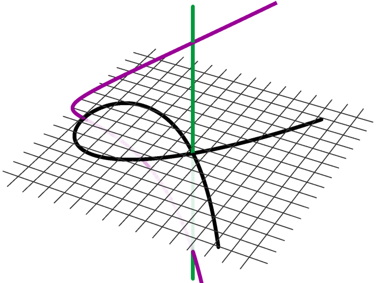
Figure 9: Left: the elliptic curve $y^{2}\!=\!x(x+0.1)(x+1)$ that is topologically a torus. Middle: the nodal curve $y^{2}\!=\!x^{2}\,(x+1)$ . Right: Blowing up the singularity. The black curve is the original nodal curve. The green line is (I) and the purple curve is (II) in Eq. (240).

Starting with the curve (236) with a small $\epsilon$ . Take the $a$ cycle to be a circle of radius $|\epsilon|$ surrounding the poles at $x=0$ and $x=-\epsilon$ , and the $b$ cycle surrounding the poles at $x=-\epsilon$ and $x=-1$ . Using the single-valued differential $dz=dx/y$ , the periods are

$$\omega_{a}=\int_{a}\frac{dx}{y}=-2\pi\,,\qquad\omega_{b}=\int_{b}\frac{dx}{y}=-2\,i\,\log\bigl{(}16\,\epsilon^{-1}\bigr{)}\,.$$ (237)

The torus modulus is given by

$$\tau=\frac{\omega_{b}}{\omega_{a}}=\frac{i}{\pi}\log\bigl{(}16\,\epsilon^{-1}\bigr{)}\,.$$ (238)

In the $\epsilon\rightarrow\infty$ limit, we find $\tau\rightarrow i\,\infty$ as in Eq. (53). Therefore, the nonrelativistic worldsheet in M0T due to the $\omega\rightarrow\infty$ limit is the same as the $\epsilon\rightarrow 0$ limit that leads to the nodal curve.

In order to understand the complex graph defined by the nodal cubic

$$y^{2}=x^{2}\,(x+1)\,,$$ (239)

we blow up the singularity by perform the change of variable $y=t\,x$ , where the parts of the nodal curve that intersect at the origin are separated, with the variable $t$ representing the slopes. Plugging $y=t\,x$ into Eq. (239), we find that the cubic factorizes into two components:

$$\text{(I)}\quad x=0\,,\quad y=0\,,\quad z=t\,;\qquad\text{(II)}\quad x=t^{2}-1\,,\quad y=t^{3}-t\,,\quad z=t\,.$$ (240)

Here, (I) is the green curve and (II) is the purple curve in the plot on the right of Fig. 9. Note that (II) This is a rational parametrization of the nodal curve. In the complex case, we write $t=u+i\,v$ , which implies

$$\text{Re}(x) =u^{2}-v^{2}-1\,, \text{Re}(y) =u^{3}-3\,u\,v^{2}-u\,,$$ (241a)

$$\text{Im}(x) =2\,u\,v\,, \text{Im}(y) =3\,u^{2}\,v-v^{3}-v\,.$$ (241b)

In Fig. 10, we draw the graph of the blown-up complex nodal curve as parametrized in Eq. (241), where it is shown that this is topologically a nodal Riemann sphere. This demonstrates that the torus becomes a nodal Riemann sphere in the $\tau\rightarrow i\,\infty$ limit.

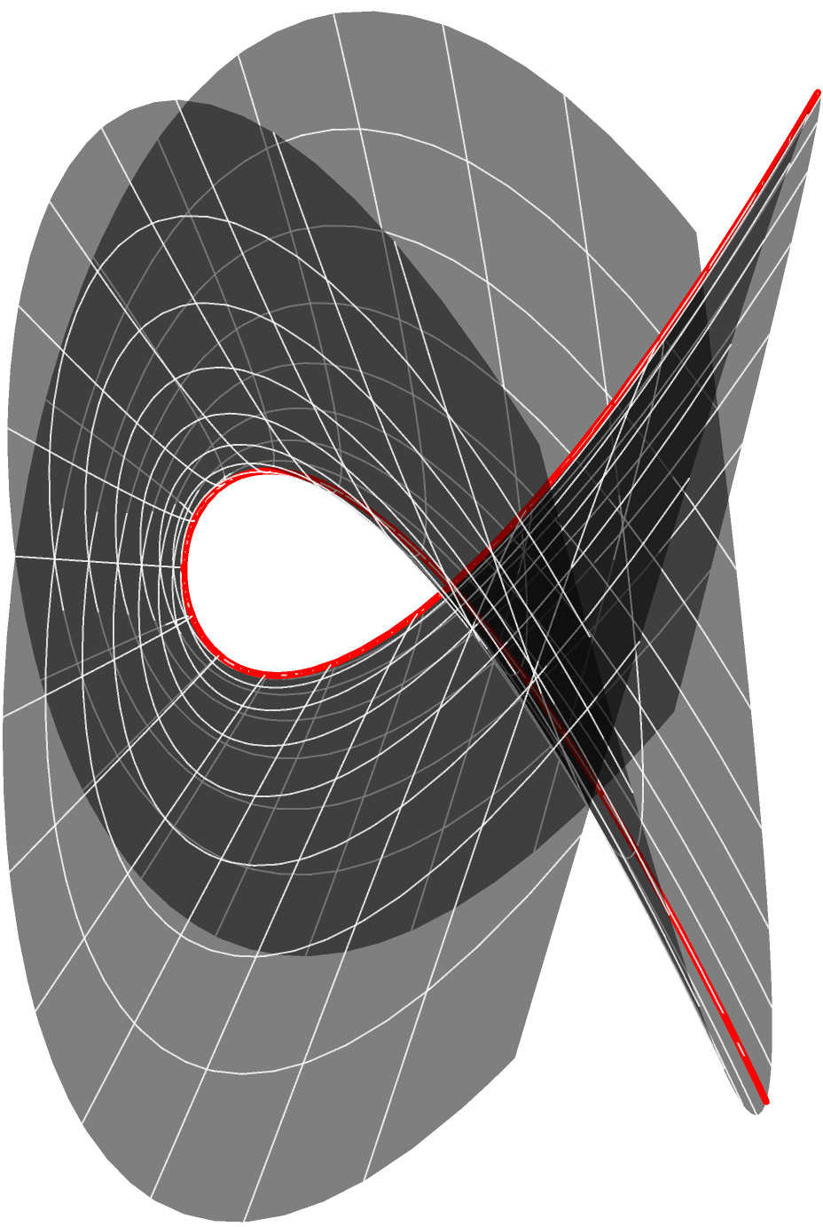
$\implies$

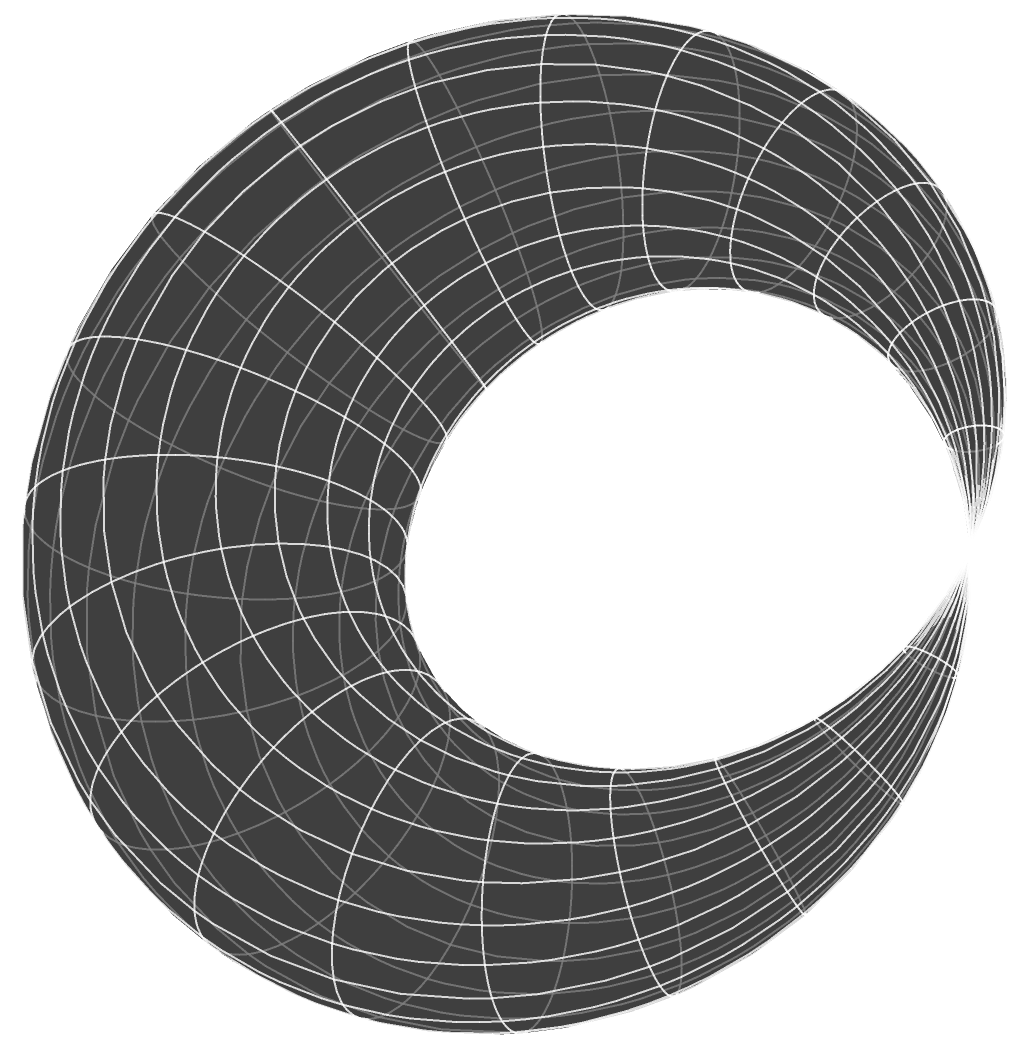
Figure 10: Left: The graph of the blown-up complex nodal curve that is parametrized in terms of $u$ and $v$ in Eq. (241). The Cartesian coordinates are $(\text{Re}(x)\,,\text{Im}(x)\,,\text{Re}(y))$ . The red curve is the real nodal curve. Right: The nodal graph on the left can be deformed into a nodal Riemann sphere after identifying the infinity as a point.

We only focused on the nodal singularity of the elliptic curve here. In the case where $p(x)$ in Eq. (236) takes a different form that has a triple root, the elliptic curve develops a singular point called cusp where there is only one tangent direction. In this case, the elliptic curve is topologically a knot.

References

- (1) P. Hořava, Membranes at quantum criticality, JHEP 03 (2009) 020, [arXiv:0812.4287].
- (2) Z. Yan, Renormalization of supersymmetric Lifshitz sigma models, JHEP 03 (2023) 008, [arXiv:2210.04950].
- (3) J. M. Maldacena, The Large N limit of superconformal field theories and supergravity, Adv. Theor. Math. Phys. 2 (1998) 231–252, [hep-th/9711200].
- (4) O. Aharony, O. Bergman, D. L. Jafferis and J. Maldacena, N=6 superconformal Chern-Simons-matter theories, M2-branes and their gravity duals, JHEP 10 (2008) 091, [arXiv:0806.1218].
- (5) L. Susskind, Another conjecture about M(atrix) theory, hep-th/9704080.
- (6) N. Seiberg, Why is the matrix model correct?, Phys. Rev. Lett. 79 (1997) 3577–3580, [hep-th/9710009].
- (7) A. Sen, D0-branes on Tn and matrix theory, Adv. Theor. Math. Phys. 2 (1998) 51–59, [hep-th/9709220].
- (8) B. de Wit, J. Hoppe and H. Nicolai, On the quantum mechanics of supermembranes, Nucl. Phys. B 305 (1988) 545.
- (9) T. Banks, W. Fischler, S. H. Shenker and L. Susskind, M theory as a matrix model: a conjecture, Phys. Rev. D 55 (1997) 5112–5128, [hep-th/9610043].
- (10) C. D. A. Blair, J. Lahnsteiner, N. A. J. Obers and Z. Yan, Unification of Decoupling Limits in String and M-theory, arXiv:2311.10564.
- (11) C. Blair, J. Lahnsteiner, N. Obers and Z. Yan, Matrix theory reloaded: U-duality, non-Lorentzian backgrounds and decoupling limits of M-theory, to appear (2023) .
- (12) R. Gopakumar, S. Minwalla, N. Seiberg and A. Strominger, OM theory in diverse dimensions, JHEP 08 (2000) 008, [hep-th/0006062].
- (13) T. Harmark, Open branes in space-time noncommutative little string theory, Nucl. Phys. B 593 (2001) 76–98, [hep-th/0007147].
- (14) J. Gomis and H. Ooguri, Nonrelativistic closed string theory, J. Math. Phys. 42 (2001) 3127–3151, [hep-th/0009181].
- (15) U. H. Danielsson, A. Guijosa and M. Kruczenski, IIA/B, wound and wrapped, JHEP 10 (2000) 020, [hep-th/0009182].
- (16) R. Dijkgraaf, J. de Boer, T. Harmark and N. A. Obers, unpublished .
- (17) C. Batlle, J. Gomis and D. Not, Extended Galilean symmetries of non-relativistic strings, JHEP 02 (2017) 049, [arXiv:1611.00026].
- (18) E. Albrychiewicz, K.-I. Ellers, A. F. Valiente and P. Hořava, Tropological sigma models, arXiv:2311.00745.
- (19) L. Mason and D. Skinner, Ambitwistor strings and the scattering equations, JHEP 07 (2014) 048, [arXiv:1311.2564].
- (20) Y. Geyer and L. Mason, The SAGEX review on scattering amplitudes Chapter 6: Ambitwistor strings and amplitudes from the worldsheet, J. Phys. A 55 (2022) 443007, [arXiv:2203.13017].
- (21) R. Dijkgraaf, E. P. Verlinde and H. L. Verlinde, Matrix string theory, Nucl. Phys. B 500 (1997) 43–61, [hep-th/9703030].
- (22) C. M. Hull, Timelike T duality, de Sitter space, large N gauge theories and topological field theory, JHEP 07 (1998) 021, [hep-th/9806146].
- (23) U. Lindstrom, B. Sundborg and G. Theodoridis, The zero tension limit of the superstring, Phys. Lett. B 253 (1991) 319–323.
- (24) J. Isberg, U. Lindstrom, B. Sundborg and G. Theodoridis, Classical and quantized tensionless strings, Nucl. Phys. B 411 (1994) 122–156, [hep-th/9307108].
- (25) N. Ishibashi, H. Kawai, Y. Kitazawa and A. Tsuchiya, A Large N reduced model as superstring, Nucl. Phys. B 498 (1997) 467–491, [hep-th/9612115].
- (26) E. Bergshoeff, J. Figueroa-O’Farrill, K. van Helden, J. Rosseel, I. Rotko and T. ter Veldhuis, -brane Galilean and Carrollian Geometries and Gravities, arXiv:2308.12852.
- (27) B. Cardona, J. Gomis and J. M. Pons, Dynamics of Carroll strings, JHEP 07 (2016) 050, [arXiv:1605.05483].
- (28) J.-M. Lévy-Leblond, Une nouvelle limite non-relativiste du groupe de Poincaré, in Annales de l’IHP Physique théorique, vol. 3, pp. 1–12, 1965.
- (29) N. Sen Gupta, On an analogue of the Galilei group, Il Nuovo Cimento A (1965-1970) 44 (1966) 512–517.
- (30) C. Duval, G. W. Gibbons, P. A. Horvathy and P. M. Zhang, Carroll versus Newton and Galilei: two dual non-Einsteinian concepts of time, Class. Quant. Grav. 31 (2014) 085016, [arXiv:1402.0657].
- (31) E. Bergshoeff, J. Gomis, B. Rollier, J. Rosseel and T. ter Veldhuis, Carroll versus Galilei Gravity, JHEP 03 (2017) 165, [1701.06156].
- (32) M. Gutperle and A. Strominger, Space-like branes, JHEP 04 (2002) 018, [hep-th/0202210].
- (33) J. Figueroa-O’Farrill, A. Pérez and S. Prohazka, Quantum Carroll/fracton particles, JHEP 10 (2023) 041, [2307.05674].
- (34) J. de Boer, J. Hartong, N. A. Obers, W. Sybesma and S. Vandoren, Carroll stories, JHEP 09 (2023) 148, [arXiv:2307.06827].
- (35) S. Pasterski, M. Pate and A.-M. Raclariu, Celestial holography, in Snowmass 2021, 11, 2021. 2111.11392.
- (36) L. Donnay, A. Fiorucci, Y. Herfray and R. Ruzziconi, Carrollian Perspective on Celestial Holography, Phys. Rev. Lett. 129 (2022) 071602, [2202.04702].
- (37) T. Harmark, J. Hartong and N. A. Obers, Nonrelativistic strings and limits of the AdS/CFT correspondence, Phys. Rev. D 96 (2017) 086019, [arXiv:1705.03535].
- (38) T. Harmark, J. Hartong, L. Menculini, N. A. Obers and Z. Yan, Strings with non-relativistic conformal symmetry and limits of the AdS/CFT correspondence, JHEP 11 (2018) 190, [arXiv:1810.05560].
- (39) T. Harmark, J. Hartong, N. A. Obers and G. Oling, Spin Matrix Theory string backgrounds and Penrose limits of AdS/CFT, JHEP 03 (2021) 129, [arXiv:2011.02539].
- (40) L. Bidussi, T. Harmark, J. Hartong, N. A. Obers and G. Oling, Longitudinal Galilean and Carrollian limits of non-relativistic strings, arXiv:2309.14467.
- (41) T. Harmark and M. Orselli, Spin Matrix Theory: A quantum mechanical model of the AdS/CFT correspondence, JHEP 11 (2014) 134, [arXiv:1409.4417].
- (42) E. Casali and P. Tourkine, On the null origin of the ambitwistor string, JHEP 11 (2016) 036, [arXiv:1606.05636].
- (43) W. Siegel, Amplitudes for left-handed strings, arXiv:1512.02569.
- (44) A. Bagchi, A. Banerjee, S. Chakrabortty, S. Dutta and P. Parekh, A tale of three–tensionless strings and vacuum structure, JHEP 04 (2020) 061, [arXiv:2001.00354].
- (45) F. Cachazo, S. He and E. Y. Yuan, Scattering of massless particles in arbitrary dimensions, Phys. Rev. Lett. 113 (2014) 171601, [arXiv:1307.2199].
- (46) F. Cachazo, S. He and E. Y. Yuan, Scattering of massless particles: scalars, gluons and gravitons, JHEP 07 (2014) 033, [arXiv:1309.0885].
- (47) Y. Geyer, L. Mason, R. Monteiro and P. Tourkine, Loop integrands for scattering amplitudes from the Riemann sphere, Phys. Rev. Lett. 115 (2015) 121603, [arXiv:1507.00321].
- (48) W. Taylor, M(atrix) theory: Matrix quantum mechanics as a fundamental theory, Rev. Mod. Phys. 73 (2001) 419–462, [hep-th/0101126].
- (49) E. Bergshoeff, E. Sezgin and P. K. Townsend, Supermembranes and eleven-dimensional supergravity, Phys. Lett. B 189 (1987) 75–78.
- (50) J. Goldstone, unpublished (1982) .
- (51) J. Hoppe, MIT PhD Thesis (1982); Quantum theory of a relativistic surface, workshop on Constraints theory and relativistic dynamics (Florence, 1986), eds. G. Longhi and L. Lusanna, 1987.
- (52) M. Baake, P. Reinicke and V. Rittenberg, Fierz identities for real Clifford algebras and the number of supercharges, Journal of Mathematical Physics 26 (1985) 1070–1071.
- (53) R. Flume, On quantum mechanics with extended supersymmetry and nonabelian gauge constraints, Annals of Physics 164 (1985) 189–220.
- (54) M. Claudson and M. B. Halpern, Supersymmetric ground state wave functions, Nucl. Phys. B 250 (1985) 689–715.
- (55) B. de Wit, M. Luscher and H. Nicolai, The supermembrane is unstable, Nucl. Phys. B 320 (1989) 135–159.
- (56) P. K. Townsend, D-branes from M-branes, Phys. Lett. B 373 (1996) 68–75, [hep-th/9512062].
- (57) E. Witten, Bound states of strings and p-branes, Nucl. Phys. B 460 (1996) 335–350, [hep-th/9510135].
- (58) J. Klusoň, Null-dimensional reduction of M2-brane, Int. J. Mod. Phys. A 37 (2022) 2250090, [arXiv:2103.00566].
- (59) P. K. Townsend, Four lectures on M theory, in ICTP Summer School in High-energy Physics and Cosmology, pp. 385–438, 12, 1996. hep-th/9612121.
- (60) E. A. Bergshoeff, K. T. Grosvenor, J. Lahnsteiner, Z. Yan and U. Zorba, Branched SL(2, ) duality, JHEP 10 (2022) 131, [arXiv:2208.13815].
- (61) R. C. Myers, Dielectric branes, JHEP 12 (1999) 022, [hep-th/9910053].
- (62) R. Gopakumar, J. M. Maldacena, S. Minwalla and A. Strominger, S duality and noncommutative gauge theory, JHEP 06 (2000) 036, [hep-th/0005048].
- (63) N. Seiberg and E. Witten, String theory and noncommutative geometry, JHEP 09 (1999) 032, [hep-th/9908142].
- (64) E. Kreyszig, Differential geometry. Courier Corporation, 2013.
- (65) P. Deligne and D. Mumford, The irreducibility of the space of curves of given genus, Publications Mathématiques de l’IHES 36 (1969) 75–109.
- (66) J.-P. Brasselet, Intersection of algebraic cycles, Journal of Mathematical Sciences 82 (1996) 3625–3632.
- (67) Y. Geyer and R. Monteiro, Two-loop scattering amplitudes from ambitwistor strings: from genus two to the nodal Riemann sphere, JHEP 11 (2018) 008, [1805.05344].
- (68) A. Bagchi, Tensionless strings and Galilean conformal algebra, JHEP 05 (2013) 141, [arXiv:1303.0291].
- (69) B. Chen, Z. Hu, Z.-f. Yu and Y.-f. Zheng, Path-integral quantization of tensionless (super) string, JHEP 08 (2023) 133, [arXiv:2302.05975].
- (70) T. Harmark, J. Hartong, L. Menculini, N. A. Obers and G. Oling, Relating non-relativistic string theories, JHEP 11 (2019) 071, [arXiv:1907.01663].
- (71) T. H. Cormen, C. E. Leiserson, R. L. Rivest and C. Stein, Introduction to algorithms. MIT press, 2022.
- (72) P. Hořava and C. J. Mogni, String perturbation theory on the Schwinger-Keldysh time contour, Phys. Rev. Lett. 125 (2020) 261602, [arXiv:2009.03940].
- (73) P. Hořava and C. J. Mogni, Keldysh rotation in the large-N expansion and string theory out of equilibrium, Phys. Rev. D 106 (2022) 106014, [arXiv:2010.10671].
- (74) P. Hořava and C. J. Mogni, Large-N expansion and string theory out of equilibrium, Phys. Rev. D 106 (2022) 106013, [arXiv:2008.11685].
- (75) A. Bagchi, R. Gopakumar, I. Mandal and A. Miwa, GCA in 2d, JHEP 08 (2010) 004, [arXiv:0912.1090].
- (76) A. Bagchi and R. Gopakumar, Galilean conformal algebras and AdS/CFT, JHEP 07 (2009) 037, [arXiv:0902.1385].
- (77) H. Bondi, M. G. J. van der Burg and A. W. K. Metzner, Gravitational waves in general relativity. 7. Waves from axisymmetric isolated systems, Proc. Roy. Soc. Lond. A 269 (1962) 21–52.
- (78) R. Sachs, Asymptotic symmetries in gravitational theory, Phys. Rev. 128 (1962) 2851–2864.
- (79) A. Bagchi, Correspondence between asymptotically flat spacetimes and nonrelativistic conformal field theories, Phys. Rev. Lett. 105 (2010) 171601, [arXiv:1006.3354].
- (80) C. Batlle, J. Gomis, L. Mezincescu and P. K. Townsend, Tachyons in the Galilean limit, JHEP 04 (2017) 120, [1702.04792].
- (81) J.-M. Souriau, Structure des systèmes dynamiques: maîtrises de mathématiques, (No Title) (1970) .
- (82) C. Duval, Z. Horvath and P. Horvathy, Geometrical spinoptics and the optical Hall effect, J. Geom. Phys. 57 (2007) 925–941, [math-ph/0509031].
- (83) C. Duval, Polarized Spinoptics and Symplectic Physics, 1312.4486.
- (84) E. Alvarez, J. L. F. Barbon and J. Borlaf, T duality for open strings, Nucl. Phys. B 479 (1996) 218–242, [hep-th/9603089].
- (85) N. A. Obers and B. Pioline, U duality and M theory, Phys. Rept. 318 (1999) 113–225, [hep-th/9809039].
- (86) J. Gomis, F. Passerini, T. Ramirez and A. Van Proeyen, Non relativistic Dp branes, JHEP 10 (2005) 007, [hep-th/0507135].
- (87) K. Kamimura and T. Ramirez, Brane dualities in non-relativistic limit, JHEP 03 (2006) 058, [hep-th/0512146].
- (88) S. Ebert, H.-Y. Sun and Z. Yan, Dual D-brane actions in nonrelativistic string theory, JHEP 04 (2022) 161, [arXiv:2112.09316].
- (89) W. Fischler, E. Halyo, A. Rajaraman and L. Susskind, The incredible shrinking torus, Nucl. Phys. B 501 (1997) 409–426, [hep-th/9703102].
- (90) S. Hyun, U-duality between NCOS theory and matrix theory, Nucl. Phys. B 598 (2001) 276–290, [hep-th/0008213].
- (91) C. M. Hull, De Sitter space in supergravity and M theory, JHEP 11 (2001) 012, [hep-th/0109213].
- (92) A. Bagchi, A. Banerjee and S. Chakrabortty, Rindler Physics on the String Worldsheet, Phys. Rev. Lett. 126 (2021) 031601, [arXiv:2009.01408].
- (93) B. Sundborg, Stringy gravity, interacting tensionless strings and massless higher spins, Nucl. Phys. B Proc. Suppl. 102 (2001) 113–119, [hep-th/0103247].
- (94) A. Bagchi, S. Chakrabortty and P. Parekh, Tensionless strings from worldsheet symmetries, JHEP 01 (2016) 158, [arXiv:1507.04361].
- (95) A. Bagchi, M. Mandlik and P. Sharma, Tensionless tales: vacua and critical dimensions, JHEP 08 (2021) 054, [arXiv:2105.09682].
- (96) A. Schild, Classical Null Strings, Phys. Rev. D 16 (1977) 1722.
- (97) F. Cachazo, S. He and E. Y. Yuan, Scattering equations and Kawai-Lewellen-Tye orthogonality, Phys. Rev. D 90 (2014) 065001, [arXiv:1306.6575].
- (98) D. J. Gross and P. F. Mende, String theory beyond the Planck scale, Nucl. Phys. B 303 (1988) 407–454.
- (99) O. Hohm, W. Siegel and B. Zwiebach, Doubled -geometry, JHEP 02 (2014) 065, [arXiv:1306.2970].
- (100) J. Hartong, Gauging the Carroll algebra and ultra-relativistic gravity, JHEP 08 (2015) 069, [arXiv:1505.05011].
- (101) D. Hansen, N. A. Obers, G. Oling and B. T. Søgaard, Carroll expansion of general relativity, SciPost Phys. 13 (2022) 055, [arXiv:2112.12684].
- (102) L. Susskind, Holography in the flat space limit, AIP Conf. Proc. 493 (1999) 98–112, [hep-th/9901079].
- (103) J. Polchinski, S matrices from AdS space-time, hep-th/9901076.
- (104) J. de Boer and S. N. Solodukhin, A Holographic reduction of Minkowski space-time, Nucl. Phys. B 665 (2003) 545–593, [hep-th/0303006].
- (105) S. Pasterski, S.-H. Shao and A. Strominger, Flat space amplitudes and conformal symmetry of the celestial sphere, Phys. Rev. D 96 (2017) 065026, [arXiv:1701.00049].
- (106) C. Dappiaggi, V. Moretti and N. Pinamonti, Rigorous steps towards holography in asymptotically flat spacetimes, Rev. Math. Phys. 18 (2006) 349–416, [gr-qc/0506069].
- (107) A. Bagchi, R. Basu, A. Kakkar and A. Mehra, Flat holography: aspects of the dual field theory, JHEP 12 (2016) 147, [arXiv:1609.06203].
- (108) K. Y. Bliokh and Y. P. Bliokh, Conservation of angular momentum, transverse shift, and spin hall effect in reflection and refraction of an electromagnetic wave packet, Physical review letters 96 (2006) 073903.
- (109) M. Onoda, S. Murakami and N. Nagaosa, Hall effect of light, Physical review letters 93 (2004) 083901.
- (110) S. Baiguera, T. Harmark, Y. Lei and Z. Yan, work in progress .
- (111) G. Oling and Z. Yan, Aspects of nonrelativistic strings, Front. in Phys. 10 (2022) 832271, [arXiv:2202.12698].
- (112) S. Baiguera, Aspects of non-relativistic quantum field theories, arXiv:2311.00027.
- (113) S. Baiguera, T. Harmark and Y. Lei, The panorama of Spin Matrix theory, JHEP 04 (2023) 075, [arXiv:2211.16519].
- (114) T. Harmark, K. R. Kristjansson and M. Orselli, Matching gauge theory and string theory in a decoupling limit of AdS/CFT, JHEP 02 (2009) 027, [arXiv:0806.3370].
- (115) J. Klusoň, Canonical analysis of non-relativistic string with non-relativistic world-sheet, Eur. Phys. J. C 82 (2022) 305, [arXiv:2101.03758].
- (116) D. Roychowdhury, Decoding the Spin-Matrix limit of strings on AdS, Phys. Lett. B 820 (2021) 136499, [arXiv:2101.06513].
- (117) M. J. Duff, H. Lu and C. N. Pope, AdS untwisted, Nucl. Phys. B 532 (1998) 181–209, [hep-th/9803061].
- (118) I. R. Klebanov and J. M. Maldacena, (1+1)-dimensional NCOS and its U(N) gauge theory dual, Adv. Theor. Math. Phys. 4 (2000) 283–302, [hep-th/0006085].
- (119) S. Ebert and Z. Yan, Anisotropic compactification of nonrelativistic M-theory, arXiv:2309.04912.
- (120) U. H. Danielsson, A. Guijosa and M. Kruczenski, Newtonian gravitons and D-brane collective coordinates in wound string theory, JHEP 03 (2001) 041, [hep-th/0012183].
- (121) F. Kristiansson and P. Rajan, Wound string scattering in NCOS theory, Phys. Lett. B 502 (2001) 235–238, [hep-th/0011054].
- (122) Z. Yan and M. Yu, KLT factorization of nonrelativistic string amplitudes, JHEP 04 (2022) 068, [arXiv:2112.00025].
- (123) J. Gomis, J. Oh and Z. Yan, Nonrelativistic string theory in background fields, JHEP 10 (2019) 101, [arXiv:1905.07315].
- (124) A. D. Gallegos, U. Gürsoy and N. Zinnato, Torsional Newton Cartan gravity from non-relativistic strings, JHEP 09 (2020) 172, [arXiv:1906.01607].
- (125) Z. Yan and M. Yu, Background field method for nonlinear sigma models in nonrelativistic string theory, JHEP 03 (2020) 181, [arXiv:1912.03181].
- (126) J. Gomis, Z. Yan and M. Yu, Nonrelativistic open string and Yang-Mills theory, JHEP 03 (2021) 269, [arXiv:2007.01886].
- (127) Z. Yan, Torsional deformation of nonrelativistic string theory, JHEP 09 (2021) 035, [arXiv:2106.10021].
- (128) B. S. Kim, World sheet commuting beta gamma CFT and non-relativistic string theories, Phys. Rev. D 76 (2007) 106007, [arXiv:0708.4261].
- (129) E. A. Bergshoeff, K. T. Grosvenor, C. Şimşek and Z. Yan, An action for extended string Newton-Cartan gravity, JHEP 01 (2019) 178, [arXiv:1810.09387].
- (130) A. D. Gallegos, U. Gürsoy, S. Verma and N. Zinnato, Non-Riemannian gravity actions from double field theory, JHEP 06 (2021) 173, [arXiv:2012.07765].
- (131) E. A. Bergshoeff, J. Lahnsteiner, L. Romano, J. Rosseel and C. Şimşek, A non-relativistic limit of NS-NS gravity, JHEP 06 (2021) 021, [arXiv:2102.06974].
- (132) C. D. A. Blair, D. Gallegos and N. Zinnato, A non-relativistic limit of M-theory and 11-dimensional membrane Newton-Cartan geometry, JHEP 10 (2021) 015, [arXiv:2104.07579].
- (133) E. A. Bergshoeff, J. Lahnsteiner, L. Romano, J. Rosseel and C. Simsek, Non-relativistic ten-dimensional minimal supergravity, JHEP 12 (2021) 123, [arXiv:2107.14636].
- (134) E. A. Bergshoeff, K. T. Grosvenor, J. Lahnsteiner, Z. Yan and U. Zorba, Non-Lorentzian IIB supergravity from a polynomial realization of SL(2, ), arXiv:2306.04741.
- (135) J. Hartong, N. A. Obers and G. Oling, Review on non-relativistic gravity, Frontiers in Physics 11 (2023) 104, [arXiv:2212.11309].
- (136) P. Hořava, Quantum gravity at a Lifshitz point, Phys. Rev. D 79 (2009) 084008, [arXiv:0901.3775].
- (137) J. Hartong and N. A. Obers, Hořava-Lifshitz gravity from dynamical Newton-Cartan geometry, JHEP 07 (2015) 155, [arXiv:1504.07461].
- (138) J. Gomis, J. Gomis and K. Kamimura, Non-relativistic superstrings: A new soluble sector of AdS, JHEP 12 (2005) 024, [hep-th/0507036].
- (139) J. Brugues, J. Gomis and K. Kamimura, Newton-Hooke algebras, non-relativistic branes and generalized pp-wave metrics, Phys. Rev. D 73 (2006) 085011, [hep-th/0603023].
- (140) R. Andringa, E. Bergshoeff, J. Gomis and M. de Roo, ‘Stringy’ Newton-Cartan gravity, Class. Quant. Grav. 29 (2012) 235020, [arXiv:1206.5176].
- (141) E. Bergshoeff, J. Gomis and Z. Yan, Nonrelativistic string theory and T-duality, JHEP 11 (2018) 133, [arXiv:1806.06071].
- (142) E. A. Bergshoeff, J. Gomis, J. Rosseel, C. Şimşek and Z. Yan, String theory and string Newton-Cartan geometry, J. Phys. A 53 (2020) 014001, [arXiv:1907.10668].
- (143) L. Bidussi, T. Harmark, J. Hartong, N. A. Obers and G. Oling, Torsional string Newton-Cartan geometry for non-relativistic strings, JHEP 02 (2022) 116, [2107.00642].
- (144) J. Hartong and E. Have, Nonrelativistic approximations of closed bosonic string theory, JHEP 02 (2023) 153, [arXiv:2211.01795].
- (145) S. M. Ko, C. Melby-Thompson, R. Meyer and J.-H. Park, Dynamics of perturbations in double field theory & non-relativistic string theory, JHEP 12 (2015) 144, [arXiv:1508.01121].
- (146) K. Morand and J.-H. Park, Classification of non-Riemannian doubled-yet-gauged spacetime, Eur. Phys. J. C 77 (2017) 685, [arXiv:1707.03713].
- (147) C. D. A. Blair, G. Oling and J.-H. Park, Non-Riemannian isometries from double field theory, JHEP 04 (2021) 072, [arXiv:2012.07766].
- (148) E. Bergshoeff, D. S. Berman, J. P. van der Schaar and P. Sundell, A noncommutative M theory five-brane, Nucl. Phys. B 590 (2000) 173–197, [hep-th/0005026].
- (149) J. A. Garcia, A. Guijosa and J. D. Vergara, A membrane action for OM theory, Nucl. Phys. B 630 (2002) 178–202, [hep-th/0201140].
- (150) J. H. Silverman, The arithmetic of elliptic curves, vol. 106. Springer, 2009.