Analysis of an iterative reconstruction method in comparison of the standard reconstruction method

Abstract

We present a detailed analysis of a new, iterative density reconstruction algorithm. This algorithm uses a decreasing smoothing scale to better reconstruct the density field in Lagrangian space. We implement this algorithm to run on the Quijote simulations, and extend it to (a) include a smoothing kernel that smoothly goes from anisotropic to isotropic, and (b) a variant that does not correct for redshift space distortions. We compare the performance of this algorithm with the standard reconstruction method. Our examinations of the methods include cross-correlation of the reconstructed density field with the linear density field, reconstructed two-point functions, and BAO parameter fitting. We also examine the impact of various parameters, such as smoothing scale, anisotropic smoothing, tracer type/bias, and the inclusion of second order perturbation theory. We find that the two reconstruction algorithms are comparable in most of the areas we examine. In particular, both algorithms give consistent fittings of BAO parameters. The fits are robust over a range of smoothing scales. We find the iterative algorithm is significantly better at removing redshift space distortions. The new algorithm will be a promising method to be employed in the ongoing and future large-scale structure surveys.

1 Introduction

The baryon acoustic oscillation (BAO) technique has become one of the most promising probes of dark energy over the last decade. BAO imprints a preferred scale in the clustering of matter and galaxies, known as the “acoustic scale”, which can be used as a standard ruler to map the expansion history of the Universe and study dark energy. This technique relies on precise measurements of the acoustic peak in configuration space, or equivalently, the wiggles in Fourier space. Ongoing and future ground-based galaxy surveys, such as DESI (DESI Collaboration et al., 2016) and Vera Rubin Observatory/LSST (LSST Science Collaboration et al., 2009), and space-based surveys, such as Euclid (Laureijs et al., 2011) and Nancy Roman Space Telescope (Spergel et al., 2013), will achieve unprecedented precision of measurements of dark energy and other cosmological parameters, thus shedding light on the nature of dark energy.

One of the systematics that impedes the precise measurements of BAO arises from the nonlinear evolution of the density field in the late-time universe, manifested in e.g., large-scale bulk flows and supercluster formation. This nonlinear evolution partially erases the acoustic peak in the matter correlation function and damps the higher harmonics in the power spectrum, reducing the accuracy of the BAO distance measurement (e.g., Meiksin et al., 1999; Seo & Eisenstein, 2005; Eisenstein et al., 2007b). Density field reconstruction aims to mitigate this effect by reversing the large-scale bulk flows. The standard reconstruction method uses Lagrangian perturbation theory to estimate the displacement of galaxies caused by nonlinear evolution and moves particles back by this distance (Eisenstein et al., 2007a). This method has been applied to data ( e.g., Padmanabhan et al., 2012; Anderson et al., 2012; Xu et al., 2013; Anderson et al., 2014a; Kazin et al., 2014; Ross et al., 2015; Beutler et al., 2015; Alam et al., 2017; Gil-Marín et al., 2020) in the past decade and has achieved improvements of precision by about a factor of 1.2-2.4 (e.g., Padmanabhan et al., 2012; Xu et al., 2013; Anderson et al., 2014a; Gil-Marín et al., 2020). However, next generation surveys could benefit from further improvement to fully realize their potential. Towards this end, there have been a number of new reconstruction methods proposed recently, aiming to obtain better results than the standard method.

Reconstruction methods can generally be categorized as Lagrangian or Eulerian, depending on whether or not moving particles back is part of the procedure. An incomplete list of Lagrangian algorithms includes the first method applied to BAO surveys, which was henceforth referred to as the standard method (Eisenstein et al., 2007a), iterative methods (e.g., Seo et al., 2010; Tassev & Zaldarriaga, 2012), iterative methods with annealing smoothing scales (e.g., Schmittfull et al., 2017), and Lagrangian methods with pixels (e.g., Seo & Hirata, 2016; Obuljen et al., 2017). An incomplete list of Eulerian algorithms involves iterative methods with annealing smoothing scales (Hada & Eisenstein, 2018) and Eulerian with growth-shift (Schmittfull et al., 2015). Among the various new ingredients, iterative approaches (e.g., Seo et al., 2010; Tassev & Zaldarriaga, 2012; Schmittfull et al., 2017; Hada & Eisenstein, 2018) aim to better resolve the difference between the Lagrangian and Eulerian positions, and varying smoothing (e.g., Schmittfull et al., 2017; Hada & Eisenstein, 2018) is designed to access smaller scales. In addition, methods may use second-order perturbation theory (e.g., Hada & Eisenstein, 2018) to attempt to reduce the inaccuracies of the approximation.

We choose Hada & Eisenstein (2018, hereafter, HE18) as representative of the new techniques to conduct detailed comparisons with the standard method (Eisenstein et al., 2007a, hereafter, ES3). The HE18 algorithm does not move particles back, but maps the density field instead. In observations, moving particles might cause mismatches across survey boundaries; thus, restoring the density field without moving particles may be a better approach. Also, it is an iterative method with decreasing (annealing) smoothing scale in each iteration. Additionally, HE18 uses the second-order perturbation theory to estimate the displacement field. However, both HE18 and ES3 share common steps, such as estimating the displacement fields.

A reconstruction algorithm can be analyzed via cross-correlation with linear density field, power spectrum and BAO fitting ability. A better reconstruction algorithm should produce a reconstructed field closer to the linear density field, a power spectrum better resembles the linear power spectrum, and resultant lower errors in BAO distance measurements. Our statistic metrics include propagator and cross-correlation of density fields, monopole power spectrum of reconstructed fields, quadrupole power spectrum in redshift space, and fittings of BAO parameters. We use Quijote simulations (Villaescusa-Navarro et al., 2019) to carry out detailed analysis that scrutinizes these aspects. We analyze the dependence of the performance on parameters, such as isotropic and anisotropic smoothing scale, number density of particles, and galaxy bias.

The structure of this paper is as follows. Section 2 summarizes the two algorithms. Section 3 presents the simulations we use. Sections 4.1 and  4.2 present analysis regarding reconstructed fields and two-point functions. Section 5 analyzes BAO fitting results. Sections 6 and 7 are discussions and conclusions. Throughout this paper, we use Quijote ’s fiducial cosmology, which is close to Planck 2018 (Aghanim et al., 2020). We use ${\bf s}$ to denote Eulerian positions and ${\bf q}$ for Lagrangian positions. The subscript $s$ denotes for redshift space.

2 Overview of reconstruction methods

We review the two reconstruction algorithms we analyze in this study in this section. Reconstruction can be done with or without removing the redshift space distortions (RSD) with the corresponding isotropic and anisotropic reconstruction conventions. We summarize first the standard algorithm, i.e. ES3 algorithm, and the new iterative algorithm, i.e. HE18, with isotropic reconstruction convention. For HE18, we also explore anisotropic smoothing, which we describe following the introduction of HE18 algorithm. We analyze anisotropic reconstruction for the two algorithms as well, and we describe the approaches in the end of this section.

2.1 ES3 reconstruction algorithm (isotropic)

The ES3 reconstruction method (Eisenstein et al., 2007a) aims to reconstruct the acoustic peak by moving particles back by their Zel’dovich displacements (Zel’Dovich, 1970). We summarize their procedure (as implemented in this paper) below.

(1) Distribute particles on a grid following Triangular Shaped Cloud (TSC) method. Calculate the density field of this grid, $\delta({\bf k})$.

(2) Compute the Zel’dovich displacement (the first order solution in Euler-Poisson systems of equations from perturbation theory) (e.g., Zel’Dovich, 1970; Buchert & Ehlers, 1993; Buchert, 1994), for the smoothed density field:

$${\bf S(k)}_{s}={\bf S(k)}+f[{\bf S(k)}\cdot{\hat{\bf z}}]{\hat{\bf z}},\\ {\bf S}({\bf k})=\frac{i({\bf k}/k^{2})\delta({\bf k})G(k)}{b(1+\beta\mu^{2})},$$ (1)

in redshift space for periodic boxes. $\delta({\bf k})$ is the density field, $b$ is the linear galaxy bias, and $\beta=f/b$, where $f$ is the linear growth rate. In redshift space, the Zel’dovich displacement in the line-of-sight direction contains the Kaiser factor, where $f$ is again the estimated linear growth rate and is set as an input parameter to study the impact of its mis-estimation. The density field is divided by bias as well as the Kaiser factor when constructed from particles. The last term, $G(k)$, is the smoothing kernel, usually assumed to be a Gaussian of width $R$:

$$G(k)=\exp\left(-\frac{1}{2}k^{2}R^{2}\right).$$ (2)

We smooth the field because small-scale data is noisy and less accurate, especially before reconstruction. The real space case is equation 1 when $f=0$.

(3) Move the original particles by $-{\bf S}({\bf k})_{s}$ and obtain the “displaced” density field, $\delta_{\rm displaced}$.

(4) Shift a set of randomly distributed particles over the same geometry. In both redshift and real space, move these randomly distributed particles by $-{\bf S}({\bf k})$ in equation 1 to form the “shifted” density field, $\delta_{\rm shifted}$. Here we adopt the isotropic reconstruction convention, where we attempt to remove the RSD by moving the particles and the randoms by different distances (c.f. anisotropic reconstruction in Section 2.3).

(5) Compute the difference of the two fields to obtain the reconstructed density field: $\delta_{r}=\delta_{\rm displaced}-\delta_{\rm shifted}$.

2.2 HE18 reconstruction algorithm (isotropic)

The HE18 method (Hada & Eisenstein, 2018) does not move particles, but instead it advects the density field. It approximates the linear density field as two parts in Lagrangian space, a large-scale part, $\delta_{l}({\bf q},t)$, and a small-scale residual part, $\delta_{\rm res}({\bf q})$: $\delta_{L}({\bf q},t)=\delta_{l}({\bf q},t)+\delta_{\rm res}({\bf q})$. Only the large-scale part, $\delta_{l}$, is assumed to cause displacement and thus changes over time, and the residual part exists from the beginning and stays the same over time. Hence, it modifies the assumption made in Lagrangian perturbation theory that the initial density everywhere is the mean density, $\rho({\bf q})={\bar{\rho}}$; instead, $\rho({\bf q})=(1+\delta_{\rm res}({\bf q})){\bar{\rho}}$. This then changes the Jacobian of the transformation between Eulerian and Lagrangian space, which is now

$$\det[\delta_{ab}^{K}+S_{a,b}]=\frac{\rho({\bf q})}{\rho({\bf s})}=\frac{1+\delta_{\rm res}({\bf q})}{1+\delta({\bf s})}.$$ (3)

Furthermore, with the assumption that only the large-scale part causes displacement, the linear solution to the Euler-Poisson system of equations becomes

$$\nabla\cdot{{\bf S}^{(1)}({\bf q})}=\nabla\cdot{{\bf S}_{l}^{(1)}({\bf q})}=-\delta_{l}({\bf q})=-\delta_{L}({\bf q})G(k),$$ (4)

where ${\bf S}_{l}^{(1)}$ is the first-order displacement of the large-scale part of the density field. The smoothed linear density is considered as the large-scale density. $G(k)$ is the smoothing kernel, equation 2, with isotropic smoothing (c.f. section 2.2.1 for anisotropic smoothing). $R$ is the smoothing scale, but it has the annealing feature in HE18, i.e., decreasing over iterations (see below), which is different from ES3’s one-step, unchanged smoothing.

The method can be described as follows:

(1) Distribute particles on a grid following TSC method. Calculate the density field of this grid $\delta_{s}({\bf s})$. This step is the same as the first step in ES3 method.

(2) Starting with the above calculated density in Eulerian space as the linear density in Lagrangian space, $\delta_{L}({\bf q})=\delta_{s}({\bf s})$ (we move to the Lagrangian space here before iterations and remain in the Lagrangian space throughout the iterations), estimate the first and second order displacements ${\bf S}_{l}^{(1)}$, ${\bf S}_{l}^{(2)}$, and ${\bf S}_{l}^{(s)}$ in the following:

$${\bf S}_{l}^{(1)}({\bf k})=\frac{i{\bf k}}{k^{2}}\delta_{L}({\bf k})G(k),$$ (5)

and

$${\bf S}_{l}^{(2)}({\bf k})=-\frac{i{\bf k}}{k^{2}}{\rm FFT}\left[-\frac{3}{14}\Omega_{m}^{-1/143}\left(S_{a,a}^{(1)}S_{b,b}^{(1)}-S_{a,b}^{(1)}S_{b,a}^{(1)}\right)\right]$$ (6)

where $S_{x,y}=\partial S_{x}/\partial q_{y}$. Here, ${\bf S}_{l}^{(1)}$ and ${\bf S}_{l}^{(2)}$ estimate the ${\bf S}^{(1)}$ and ${\bf S}^{(2)}$, the first (or Zel’dovich displacement) and second orders of solutions to the Euler-Poisson system of equations, by the aforementioned assumption. Iterations start with an ${\bf S}^{(1)}$ that is the same as ${\bf S}({\bf k})$ in the ES3 method in equation 1, except that only the bias $b$, but not the Kaiser factor, is being corrected for the density, i.e. $\delta_{L}({\bf k})=\delta({\bf k})/b$. Redshift space distortions are being accounted for through iterative estimations of the displacement. Although equation 5 is only valid in linear theory and our pre-reconstruction density contains RSD, the iterations will converge regardless of where the input position is.

In order to better access smaller scales, we decrease the smoothing scale using the prescription in HE18 and Schmittfull et al. (2017):

$$R_{n}={\rm max}\left(\frac{R_{\rm ini}}{\mathcal{D}^{n}},R_{\rm eff}\right),$$ (7)

where subscript $n$ denotes iteration number. $R_{\rm ini}$ is the smoothing scale we start iterations with and we use $R_{\rm ini}=20\ h^{-1}\ \rm{Mpc}$ in all cases. $\mathcal{D}$ is the annealing factor. We use 1.2 for our tests. If the smoothing scale reaches the effective smoothing and the iteration has not converged, the algorithm runs at the effective smoothing for the remaining iterations.

With ${\bf S}_{l}^{(1)}$ and ${\bf S}_{l}^{(2)}$ calculated, we can obtain the total displacement:

$${\bf S}_{l}({\bf q},t)={\bf S}_{l}^{(1)}+{\bf S}_{l}^{(2)}$$ (8)

in real space and

$$~{}{\bf S}_{l,s}({\bf q},t)={\bf S}_{l}^{(1)}+{\bf S}_{l}^{(2)}+\beta[({\bf S}_{l}^{(1)}+2{\bf S}_{l}^{(2)})\cdot{\hat{{\bf z}}}]{\bf{\hat{z}}}$$ (9)

in redshift space.

(3) Update the linear density following

$$\begin{split}\delta_{L,n,{\rm pre-weighted}}({\bf q},t)&=\det\left[\delta_{ab}^{K}+S_{l,s,n|a,b}\right]\times\left(1+\delta_{s,n}({\bf s[{\bf q}]})\right)\\ &-\left(1+\mu_{1}({\bf S}_{l,n-1}^{(1)}({\bf q}))\right)\end{split}$$ (10)

through iterations until the linear density field converges. $n$ is again the iteration number. Here,

$$\mu_{1}({\bf S}_{l}^{(1)})=\nabla\cdot{\bf S}_{l}^{(1)}=-\delta_{l}({\bf q}).$$ (11)

In real space, substitute ${\bf S}_{l|a,b}$ for ${\bf S}_{l,s|a,b}$. Note that the method starts with final Eulerian particle position s, but the estimated linear density field is in terms of the initial, Lagrangian particle position q. $\delta_{s}({\bf s})$ is unsmoothed, while $\mu_{1}({\bf S}_{l}^{(1)})$ and ${\bf S}_{l,s|a,b}$ (or ${\bf S}_{l|a,b}$) are both smoothed. One place we modify from HE18 original algorithm is that we calculate the above determinant directly, instead of expressing it in terms of the derivatives of ${\bf S}_{l}^{(s)}$.

(4) Weigh the calculated $n$-th density field:

$$\delta_{L,n}=w\delta_{L,n,{\rm pre-weighted}}+(1-w)\delta_{L,n-1},$$ (12)

where $w$ is the weight, which takes a value between 0 and 1. $w$ varies according to the smoothing scale. The particular choices of weights that we use (corresponding to different smoothing scales) is specified below.

The convergence criterion is

$$r_{\rm con}=\frac{\sum[\delta_{L,n}-\delta_{L,n-1}]^{2}}{\sum\delta_{s}^{2}}<0.01,$$ (13)

where the subscript $n$ represents the iteration number and the summation is over all the grid cells. $\delta_{s}$ is the unsmoothed pre-reconstruction density.

2.2.1 Anisotropic smoothing

The smoothing described above is isotropic. However, due to RSD along line of sight, we might benefit from an anisotropic smoothing. Following HE18, we introduce a parameter that quantifies the different smoothings along line of sight and perpendicular to line of sight:

$$C_{\rm ani}=R_{\parallel}/R_{\perp},$$ (14)

where $R_{\parallel}$ and $R_{\perp}$ represent the smoothing scale in the direction parallel and perpendicular to line of sight, respectively. Accordingly, the anisotropic smoothing becomes

$$G_{\rm ani}(k)=\exp[-\frac{1}{2}(k_{\perp}^{2}+k_{\parallel}^{2}C_{\rm ani}^{2})R_{\perp}^{2}].$$ (15)

The effective smoothing in the isotropic case corresponds to the perpendicular to line-of-sight smoothing, $R_{\perp}$. We analyze two cases for HE18, one with fixed $C_{\rm ani}$ over iterations, and the other with annealing $C_{\rm ani}$, which decreases by a factor of 1.1 every iteration until it becomes 1:

$$C_{{\rm ani},n}={\rm max}\left(\frac{C_{\rm ani,ini}}{1.1^{n}},1\right).$$ (16)

We attempt to reduce the smoothing needed along the line of sight, because the effects of RSD decrease over iterations where RSD is gradually being removed.

We analyze both algorithms with smoothing scales 15, 10, and 7.5 $h^{-1}\ \rm{Mpc}$ for isotropic smoothing. For anisotropic smoothing analysis, $R_{\perp}$ are fixed at these values and $C_{\rm ani}$ (or $C_{\rm ani,ini}$, in the case of annealing $C_{\rm ani}$) varies from 1 to 2.5. The weight $w$ is taken to be 0.7, 0.5, and 0.4, corresponding to the above smoothing scales.

2.3 Anisotropic reconstruction

Our regular reconstruction (with isotropic and anisotropic smoothing) in redshift space is isotropic, meaning that we attempt to remove redshift space distortions in the final reconstructed field. Since reconstruction does not completely remove RSD, we explore an alternative reconstruction approach where we do not remove RSD and can thus better model the output. We examine the performance of the two algorithms in redshift space when RSD is not removed.

For HE18, we use the same pre-reconstruction density field (not divided by the Kaiser factor) to calculate the displacement field. We calculate the displacement without the redshift space part in equation 9:

$${\bf S}_{l}({\bf q},t)={\bf S}_{l}^{(1)}+{\bf S}_{l}^{(2)},$$ (17)

effectively the same as equation 8 for real space. For ES3, we also use the same pre-reconstruction density field, which is divided by the Kaiser factor. We move both the displaced and the shifted density fields by the same amount,

$${\bf S(k)}_{s}={\bf S(k)}+f[{\bf S(k)}\cdot{\hat{\bf z}}]{\hat{\bf z}}.$$ (18)

This is one convention for anisotropic reconstruction (e.g., Seo & Eisenstein, 2007; Chen et al., 2019, denoted as RecSym) (c.f. different conventions in Seo et al. (2010); Mehta et al. (2011); Seo et al. (2016)).

3 Overview of simulations used

We use the Quijote simulations (Villaescusa-Navarro et al., 2019) to conduct our analysis. The Quijote simulations are a large suite of full $N$-body simulations run with TreePM Gadget-III for three different resolutions in boxes of 1 $h^{-1}$Gpc using a cosmology close to Planck 2018 cosmology (Aghanim et al., 2020): $\Omega_{\rm m}=0.3175$, $\Omega_{\rm b}=0.049$, $h=0.6711$, $n_{s}=0.9624$, $\sigma_{8}=0.834$, $M_{\nu}=0.0\$eV, and $w=-1$. We use the 100 high-resolution (1024³ CDM particles) simulations with both snapshots as matter fields and halo catalogs as halo fields at redshift $z=0$ and 1. We focus on two mass bins for the halo fields, $10^{12.5}-10^{13}h^{-1}\ M_{\odot}$ and $10^{13}-10^{13.5}h^{-1}\ M_{\odot}$. The number densities for the two mass bins are $1.0\times 10^{-3}h^{-1}\ \rm{Mpc}^{3}$ and $3.7\times 10^{-4}h^{-1}\ \rm{Mpc}^{3}$ at $z=0$, and $8.6\times 10^{-4}h^{-1}\ \rm{Mpc}^{3}$ and $2.3\times 10^{-4}h^{-1}\ \rm{Mpc}^{3}$ at $z=1$, respectively. We estimate the bias for the two mass bins to be 0.92 and 1.12 at $z=0$, and 1.70 and 2.29 at $z=1$, respectively.

4 Comparisons of the reconstructed fields

As described above, the reconstruction algorithms have a number of parameters that can be tuned. In this section, we examine the performance of the algorithms as function of these parameters at the level of the reconstructed density fields. While we will compare the ES3 and HE18 algorithms as part of this, we defer a more detailed comparison to Sec. 6.4.

4.1 Propagators and cross-correlations

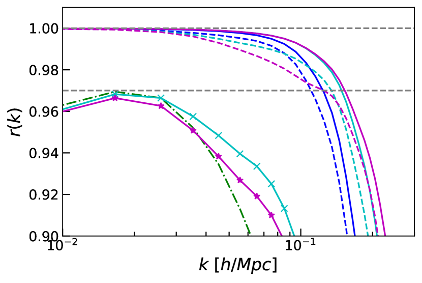
Figure 1: The cross-correlation $r(k)$ with the initial density field for lower-mass bin halo and matter fields at $z=0$ in redshift space. Solid lines are HE18 matter field, dashed lines are ES3 matter field, crosses are HE18 halo field, stars are ES3 halo field. The colors - blue, cyan and magenta represent 15, 10, and 7.5 $h^{-1}\ \rm{Mpc}$ smoothing. The horizontal dashed lines are the expected $r(k)$ values as $k\rightarrow 0$. For halos, this value is less than 1 due to shot noise. In general, we find that decreasing the smoothing scale improves the overall cross-correlation with the initial density field. However, this improvement appears to reach a maximum at $\sim 10h^{-1}\ \rm{Mpc}$ for the ES3 algorithm, after which the cross-correlation coefficient starts to get distorted. The HE18 algorithm does not appear to show this behavior. We find similar trends with smoothing for the halo fields, although we do not see any distortions in $r(k)$ in the ES3 algorithm at the smoothing scales we consider. We only show the results for the $7.5h^{-1}\ \rm{Mpc}$ smoothing scale for ES3, and the $10h^{-1}\ \rm{Mpc}$ smoothing scale for HE18 for clarity. As a reference, the dash-dotted line shows the cross-correlation with the unreconstructed halo field.

The goal of reconstruction is to recover the linear density field, and so, the simplest (two-point) statistic to examine is the cross-correlation between the reconstructed and linear density fields. There are two ways to normalize this cross-correlation. The first is the standard cross-correlation coefficient $r(k)$ defined as

$$r(k)=\frac{\left<\delta^{*}(k)\delta_{\rm ini}(k)\right>}{\sqrt{\left<\delta^{2}(k)\right>\left<\delta^{2}_{\rm ini}(k)\right>}}$$ (19)

where $\delta(k)$ and $\delta_{\rm ini}(k)$ are the reconstructed and the initial densities in Fourier space, respectively. Note that $r(k)$ is strictly bounded between $-1$ and $1$, and the closer it is to $1$, the better the reconstruction. However, $r(k)$ is not sensitive to the overall ($k$-dependent) amplitude of the reconstructed field, but it measures how well reconstruction has recovered the phases of the initial density field.

A second normalization is the propagator $G(k)$, which is defined as

$$G(k)=\frac{\left<\delta^{*}(k)\delta_{\rm ini}(k)\right>}{\left<\delta^{2}_{\rm ini}(k)\right>}$$ (20)

This is commonly used in studies of reconstructing the BAO feature since it characterizes the nonlinear damping of the BAO feature. Initial studies of reconstruction (Eisenstein et al., 2007b; Padmanabhan & White, 2009) modeled this as a Gaussian. A more recent study (Seo et al., 2016) showed that a modification to a simple Gaussian form can better account for the impact of the reconstruction smoothing scale. They propose a form for the propagator

$$G(k,\mu)=(1+\beta\mu^{2}\Sigma_{R})\exp\left[-\frac{1}{4}\left(k^{2}\mu^{2}\Sigma_{\parallel}^{2}+k^{2}(1-\mu^{2})\Sigma_{\perp}^{2}\right)\right],\\$$ (21)

where $\Sigma_{R}=1$ before reconstruction and

$$\Sigma_{R}=1-\exp[-k^{2}R^{2}/2]$$ (22)

after reconstruction. The parameters $\Sigma_{\parallel}$ and $\Sigma_{\perp}$ describe the BAO damping in the line-of-sight and transverse directions, respectively, while $R$ is related to the reconstruction smoothing scale. Measuring the propagator and these three parameters allow us to quantify the impact of reconstruction on the BAO feature. To avoid fitting to the full 2d shape of the propagator, we fit the $l=0,2$ multipoles defined by

$$G_{l}(k)=\frac{2l+1}{2}\int_{-1}^{1}G(k,\mu)L_{l}(\mu)\text{d}\mu\,,$$ (23)

where $L_{l}(\mu)$ is the Legendre polynomial.

Finally, we note that the ratio of $G(k)$ to $r(k)$ is the square-root of the ratio of the reconstructed power spectrum to the linear power spectrum as well.

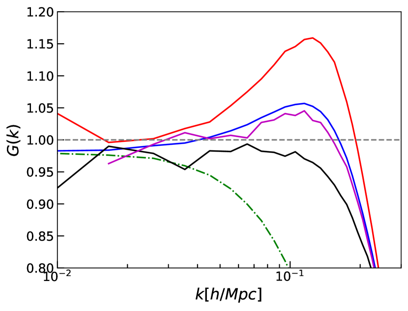
Figure 2: The propagator $G(k)$ as a function of angle, shown here for the lower mass halo field in redshift space. The field is reconstructed using HE18 with a 15 $h^{-1}\ \rm{Mpc}$ effective smoothing scale, with qualitatively similar results for other smoothing scales, as well as the ES3 algorithm. The black, magenta and red lines correspond to angular wedges of $\mu<1/3$ (perpendicular to line-of-sight), $1/3<\mu<2/3$, and $\mu>2/3$ (parallel to line-of-sight), respectively, where $\mu=|k_{z}/k|$. The blue line shows the angle-averaged $G(k)$. The green dash-dotted line is the propagator before reconstruction (in redshift space) for comparison. The angle groups show some noise, but we observe anti-correlations among them. The shape of the propagator and in particular, the bump around $k=0.1h^{-1}\ \rm{Mpc}$ can clearly be seen as coming from redshift space distortions, and this shape is captured by the modified Gaussian model presented in the text.

We start by measuring $r(k)$ and $G(k)$ as a function of the reconstruction smoothing scale. Fig. 1 plots $r(k)$ for different smoothing scales for different algorithms, for both the matter and halo density fields. In general, we find that the cross-correlation improves with decreasing smoothing scales. However, this improvement starts to saturate at $\sim 10h^{-1}\ \rm{Mpc}$ in matter field. At smaller smoothing, the ES3 $r(k)$ starts to get more distorted at intermediate $k\sim 0.1h^{-1}\ \rm{Mpc}^{-1}$ scales.

Characterizing $G(k)$ is more challenging, since it is not bounded between $-1$ and $1$. In particular, as can be seen from the functional form of the propagator presented in Eqn. 21, the propagator is expected to exceed 1 due to RSD as one looks along the line of sight. Fig. 2 shows $G(k)$ as a function of angle to the line of sight for a fixed smoothing scale of 15 $h^{-1}\ \rm{Mpc}$ for the HE18 algorithm. The “bump” in the propagator due to RSD can clearly be seen. Furthermore, this bump gets more pronounced as one increases the smoothing scale, as expected from the Gaussian model for the propagator. Therefore, we fit the $l=0$ and $l=2$ multipoles of the propagator to our model (Eqns. 21- 23) and use the fitted parameters to characterize the impact of reconstruction. Fig. 3 shows these results. As with $r(k)$, we see a decrease in the damping parameters with decreasing smoothing scale (corresponding to a better cross-correlation), and that the improvements are most noticeable going from the case of the unreconstructed density field to any of the reconstructed cases. The differences between the two algorithms are less clear. We present the fits for $G(k)$ (with 7.5 $h^{-1}\ \rm{Mpc}$ smoothing scale) in Table 1. The ES3 model appears to perform better for modes perpendicular to the line of sight, but the trend is unclear in the parallel to the line of sight. However, the differences between the two algorithms are small, relative to the improvements over the unreconstructed field. Table 1 summarizes the fitted parameters of the propagator for the different fields and algorithms.

Figure 3: Estimated $\Sigma_{\parallel}$ as a function of smoothing scale, from fitting the monopole and quadrupole of the propagator with model presented in the text. Points connected by blue lines are for the HE18 method, while those with magenta lines are for the ES3 method. From top to bottom, the lines correspond to the $z=0$ matter field, the $z=0$ lower mass halo field, and the $z=1$ lower mass halo field. Also shown are the values of $\Sigma_{\parallel}$ before reconstruction (at a smoothing scale of $\infty$). Reconstruction clearly reduces the overall damping, although we do not find a clear trend with the type of algorithm used.

field	redshift	sample	$\Sigma_{\perp}$	$\Sigma_{\parallel}$
matter	0	pre-recon	8.1	12.8
		HE18	4.5	6.1
		ES3	4.1	7.1
	1	pre-recon	5.2	9.9
		HE18	3.1	5.6
		ES3	2.8	5.8
halo lower mass bin	0	pre-recon	7.8	12.1
		HE18	3.6	5.6
		ES3	3.1	5.9
	1	pre-recon	4.8	9.2
		HE18	2.4	5.1
		ES3	1.9	4.6
halo higher mass bin	0	pre-recon	7.6	11.8
		HE18	3.7	6.2
		ES3	3.1	5.9
	1	pre-recon	4.7	9.1
		HE18	2.7	5.7
		ES3	2.1	4.8

Table 1: The damping scales from the propagator for matter and halo fields in redshift space for both reconstruction methods at $z=0$ and 1, using the modified Gaussian model described in the text. The fits here are for the case of 7.5 $h^{-1}\ \rm{Mpc}$ smoothing. We find a mild dependence on the smoothing scale, summarized in Fig. 3.

Figure 4: The propagator $G(k)$ and cross-correlation coefficient $r(k)$ of the matter field at $z=0$ in redshift space with anisotropic smoothing from HE18. All of these cyan lines have 10 $h^{-1}\ \rm{Mpc}$ smoothing perpendicular to the line-of-sight direction. The solid, dashed, dash-dotted, cross, dotted, and starred lines represent cases with $C_{\rm ani}$=1.0 (isotropic), 1.3, 1.6, 1.9, 2.2, and 2.5. In general, increasing the anisotropy in the smoothing reduces $r(k)$, and increases the RSD feature in $G(k)$ discussed earlier. For this particular case, we find the best agreement with the initial conditions for $C_{\rm ani}\sim 1.6$. The trends in both $G(k)$ and $r(k)$ here also present in ES3.

The angle dependence of the propagator suggests exploring the impact of an anisotropic smoothing kernel before reconstruction. Fig. 4 shows $G(k)$ and $r(k)$ as a function of the anisotropic smoothing parameter $C_{\rm ani}$ defined above, with smoothing along perpendicular line of sight fixed at 10 $h^{-1}\ \rm{Mpc}$. We find that including a moderately larger smoothing scale along the line of sight can result in an improved $G(k)$ closer to 1, without a significant degradation in $r(k)$. The figure shows this effect for the HE18 algorithm and the matter density field, but similar results can be seen for other tracers and the ES3 algorithm. However, the exact degree of smoothing/anisotropy that is optimal does appear to depend on the tracer used. So, one way to optimize the smoothing for $G(k)$ can be finding a relatively small isotropic smoothing scale such that the bump does not present and then finding an $C_{\rm ani}$ that gets $G(k)$ closer to 1.

Finally, we note that both the HE18 and ES3 algorithms perform similarly when benchmarked against the unreconstructed density field. In general, the HE18 algorithm performs somewhat better in the $r(k)$ statistic, and appears to be more stable when reducing the smoothing scale. This is likely a reflection of the iterative nature of the HE18 algorithm gradually reducing the smoothing scale. Using too small a smoothing scale risks a breakdown in the simple model used to reconstruct the displacement field.

4.2 Power spectrum

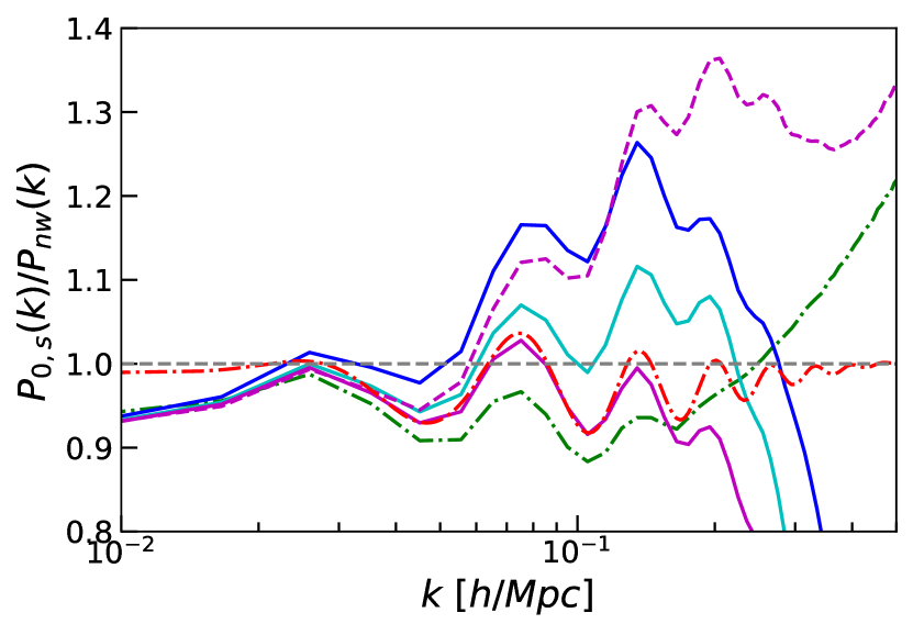
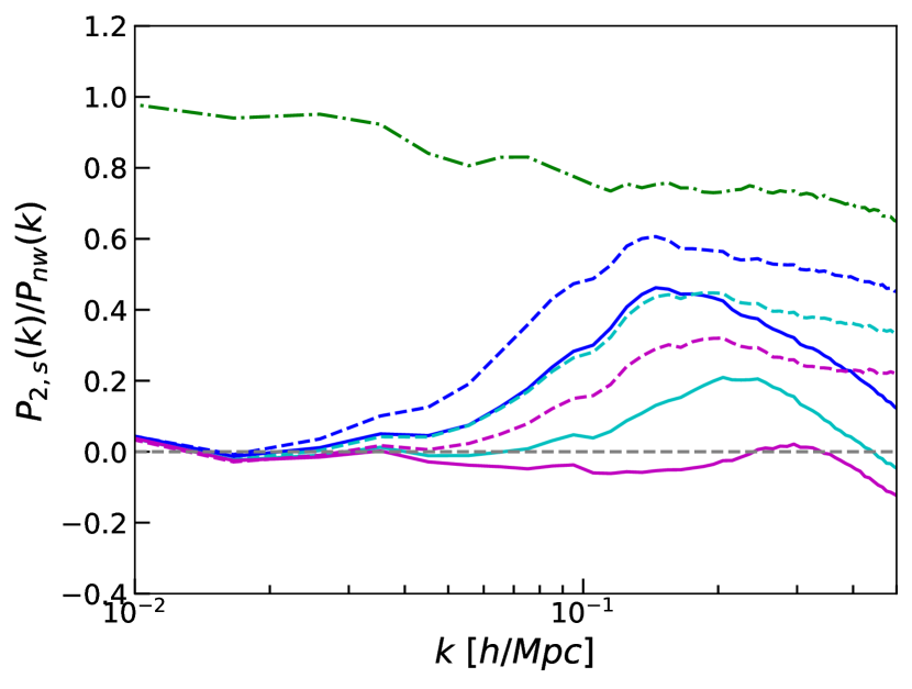
Figure 5: The monopole (left) and quadrupole (right) power spectra for the lower mass halo field at $z=0$ in redshift space. To highlight the BAO feature, we divide the power spectra by a smooth power spectrum that approximately matches the shape of the linear theory without any BAO features present. When plotting the unreconstructed fields, we also account for linear redshift space distortions using the Kaiser approximation, explaining why the ratio of power spectra goes to 1 on large scales. Since our default implementation of the HE18 and ES3 models correct for RSD, we do not need anything further for the reconstructed fields. The solid lines show the HE18 algorithm, while the dashed lines are the ES3 algorithm. The green dash-dotted line shows the unreconstructed power spectra. The left panel also shows the linear theory power spectrum (red dash-dotted lines). The different colors correspond to different smoothing scales: blue: 15 $h^{-1}\ \rm{Mpc}$, cyan: 10 $h^{-1}\ \rm{Mpc}$, magenta: 7.5 $h^{-1}\ \rm{Mpc}$. For clarity, we only show the 7.5 $h^{-1}\ \rm{Mpc}$ smoothing for the ES3 monopole. Larger smoothing scales show even larger residual nonlinear effects. We observe that the HE18 algorithm with a smoothing scale of 7.5 $h^{-1}\ \rm{Mpc}$ results in a monopole power spectrum that most closely matches linear theory (out to $k\sim 0.1h^{-1}\ \rm{Mpc}^{-1}$), and a quadrupole that is closest to zero (consistent with the removal of RSD).

Next we examine the monopole power spectrum of the reconstructed field. The patterns in monopole across different fields are similar, so again we show the lower mass bin of the halo fields at $z=0$ as an example. The left panel of Figure 5 shows the monopole before/after reconstruction with various smoothing scales in redshift space. While both the HE18 and ES3 algorithms effectively reconstruct the BAO features (that are more prominently seen compared with the unreconstructed field), the ES3 algorithm does not capture the broadband shape of the power spectrum as well. In particular, we see excess power at $k\sim 0.1h^{-1}\ \rm{Mpc}^{-1}$ for the ES3 algorithm and this excess power increases with increasing smoothing scale (not shown in the figure for clarity). By contrast, the HE18 algorithm does a better job of reconstructing the broadband shape of the power spectrum, especially with smaller smoothing scales. This is consistent with the results from the propagator and cross-correlations that we discussed earlier.

We also examine the performance of the two algorithms in removing redshift space distortions, as measured by the quadrupole power spectrum. In redshift space, the quadrupole is non-zero due to redshift space distortions; on large scales, from the Kaiser effect and on small scales, from Finger-of-God effects. A perfect reconstruction would ideally remove all the redshift space distortions due to Kaiser effect, returning a vanishing quadrupole on large scales. The right panel of Figure 5 shows the quadrupole power for the lower mass bin halo field at $z=0$ in redshift space. We find HE18 performs significantly better than ES3, bringing the quadrupole closer to zero. Similar behavior is seen for different tracers at different redshifts. Removing redshift space distortions is HE18’s strongest advantage in our analyses. This improvement in removing redshift space distortions is also indicated in Duan & Eisenstein (2019) with analysis in configuration space.

5 Fitting BAO parameters

The previous sections compared the two reconstruction methods at the level of the measured two-point statistics, especially in cross-correlation with the initial density field. These comparisons are relevant if the goal is to accurately estimate the initial linear density field. However, the initial motivation behind reconstruction was to increase the S/N of BAO measurements. This is a weaker requirement than reconstructing the initial density field - we just require that we measure the BAO distance scale with a smaller bias and error than would be possible with the unreconstructed data (c.f. recent work aiming to recover the linear density field for a larger scale range, e.g. Chen et al. (2023); Shallue & Eisenstein (2023)). In what follows, we compare the inferred distance errors and biases for both reconstruction methods.

5.1 Method

5.1.1 Power Spectrum Template

The traditional approach to measuring BAO distances is to compare the observed power spectrum/correlation function with a shifted/distorted theoretical template of the same. The shifts/distortions measure distances (as we review below), while the template captures the effects of nonlinear evolution, redshift space distortions and reconstruction.

While it is possible to use a more theoretically motivated template for standard reconstruction (e.g., Padmanabhan et al., 2009; Noh et al., 2009; White, 2014; Chen et al., 2019; Seo et al., 2021), no such modelling exists as yet for HE18 (c.f. Seo et al. (2021) for the treatment for a different iterative reconstruction method).

For the uniformity of comparisons, we use a phenomenologically motivated template (Eisenstein et al., 2007b; Anderson et al., 2012, 2014b; Beutler et al., 2016; Gil-Marín et al., 2020) that has formed the basis of most recent BAO analyses. One of the results of this work is therefore the tuning and validation of this template for the HE18 reconstruction method.

The 2D power spectrum template is

$$P^{\rm temp}(k,\mu)=(1+\beta\mu^{2}\Sigma_{R})^{2}F(k,\mu,\Sigma_{s})P^{\rm dw}(k,\mu).$$ (24)

The first term describes the Kaiser effect caused by galaxies infalling towards the cluster center on large scales (Kaiser, 1987) and $\beta=f/b$, where $f$ is the growth factor and $b$ is linear galaxy bias. We use a $\Sigma_{R}$-parameter to account for the removal of RSD in reconstruction:

$$\Sigma_{R}=1-\exp[-k^{2}R^{2}/2].$$ (25)

$\Sigma_{R}$ is set to 1 before reconstruction (Beutler et al., 2016; Seo et al., 2016). This function captures the effect of the smoothing scale used in reconstruction. Note that the addition of $\Sigma_{R}$ is identical to what we used in the modified Gaussian model for the reconstructed propagator. While $R$ could be simply fixed to the smoothing scale, we find that we get better fits when we allow it to vary. This is especially true for the HE18 algorithm, where the smoothing scale is not fixed, but gradually decreases over the course of the algorithm’s iterations. The second term represents the finger-of-God (FoG) effect caused by random velocities within virialized clusters on small scales (Park et al., 1994; Peacock & Dodds, 1994). We use the model

$$F(k,\mu,\Sigma_{s})=\frac{1}{(1+k^{2}\mu^{2}\Sigma_{s}^{2}/2)^{2}},$$ (26)

where $\Sigma_{s}$ is the FoG parameter characterizing the dispersion due to random peculiar velocities. The de-wiggled power spectrum $P^{\rm dw}$ has the form

$$\begin{split}P^{\rm dw}(k,\mu)&=P^{\rm nw}(k)\times\\ &\left(1+(O^{\rm lin}(k)-1)\times\exp\left[-\frac{1}{2}\left(k^{2}\mu^{2}\Sigma_{\parallel}^{2}+k^{2}(1-\mu^{2})\Sigma_{\perp}^{2}\right)\right]\right),\end{split}$$ (27)

where $O^{\rm lin}(k)$ is the ratio of the linear power spectrum and the linear power spectrum with BAO wiggles smoothed out: $O^{\rm lin}(k)=P^{\rm lin}(k)/P^{\rm nw}(k)$. Our $P^{\rm nw}(k)$ is a smoothed fit with polynomials for the no-wiggle power spectrum form of Eisenstein & Hu (1998). The exponential term on the far right models the damping of BAO due to nonlinear evolution. In redshift space, this damping is anisotropic, and $\Sigma_{\parallel}$ and $\Sigma_{\perp}$ are the streaming scales along and perpendicular to line of sight, respectively. For real space, the redshift-space associated terms all vanish, including $f$ (in the Kaiser term) and the high-order multipoles, and the streaming scales reduce to one parameter: $\Sigma_{\parallel}=\Sigma_{\perp}$.

We expand this 2D template into Legendre multipoles

$$P^{\rm temp}_{l}(k)=\frac{2l+1}{2}\int_{-1}^{1}P^{\rm temp}(k,\mu)L_{l}(\mu)\text{d}\mu.$$ (28)

where $L_{l}$ is the Legendre polynomial, with $l$ denoting the degree. We use both monopole and quadrupole in the fitting procedure.

As in standard BAO analyses, we also introduce a set of nuisance parameters to account for errors in the fiducial cosmology, observational systematics, and mismatches between the broadband shape of our template and the observations. Our final functional form is

$$P^{\rm fit}_{l}(k)=B^{2}P^{\rm temp}_{l}(k)+\mathcal{A}_{l}(k),$$ (29)

where $B^{2}$ characterizes the linear galaxy bias. Note that we only fit one $B^{2}$ parameter for both monopole and quadrupole in redshift space. $\mathcal{A}_{l}$ are polynomials with nuisance parameters, and We use

$$\mathcal{A}_{l}(k)=A_{l,1}k^{2}+A_{l,2}k+A_{l,3}+\frac{A_{l,4}}{k}+\frac{A_{l,5}}{k^{2}}+\frac{A_{l,6}}{k^{3}}$$ (30)

where $A_{l,1}$-$A_{l,6}$ are nuisance parameters for each multipole power spectrum.

5.1.2 Distance parameters

To measure $D_{A}(z)$ and $H(z)$, one needs to assume a fiducial cosmology to translate a measured sky position and redshift to Cartesian coordinates. This fiducial cosmology may deviate from the true cosmology (in the case of simulations, the cosmology used to generate the simulation data) one aims to measure. We can measure this deviation by estimating two parameters, isotropic dilation, $\alpha$, and anisotropic warping, $\epsilon$ (Padmanabhan & White, 2008). However, these two parameters couple the cosmological parameters, $D_{A}(z)$ and $H(z)$, that we aim to measure. So we compute another set of parameters, $\alpha_{\parallel}$ and $\alpha_{\perp}$, which decouple the cosmological parameters and are thus favored in observational analysis recently (e.g., Beutler et al., 2016). In real space, we still measure $\alpha$ ($\epsilon$ vanishes). These two sets of parameters are related to $D_{A}(z)$ and $H(z)$ in the form of

$$\alpha=\left[\frac{D_{A}^{2}(z)H_{f}(z)}{D_{A,f}^{2}(z)H(z)}\right]^{1/3}\frac{r_{s,f}}{r_{s}},1+\epsilon=\left[\frac{H_{f}(z)D_{A,f}(z)}{H(z)D_{A}(z)}\right]^{1/3},$$ (31)

$$\alpha_{\parallel}=\frac{H_{f}(z)r_{s,f}(z)}{H(z)r_{s}(z)},\alpha_{\perp}=\frac{D_{A}(z)r_{s,f}(z)}{D_{A,f}(z)r_{s}(z)},$$ (32)

where $r_{s}$ is sound horizon and subscript $f$ stands for fiducial. These two sets are related in this form: $\alpha_{\parallel}=\alpha(1+\epsilon)^{2}$ and $\alpha_{\perp}=\alpha/(1+\epsilon)$. When the fiducial cosmology perfectly matches the true cosmology, $\alpha=1$ and $\epsilon=0$, and $\alpha_{\parallel}=\alpha_{\perp}=1$. Measuring these parameters in simulations allows us to estimate any biases in the reconstruction, to forecast estimated errors, and to compare the efficacy of different reconstruction schemes.

5.1.3 Fitting Procedure

With the above construction, we proceed to fitting by minimizing $\chi^{2}$, following an approach similar to Xu et al. (2012) and Xu et al. (2013). We have in total 13 parameters in redshift space and 7 parameters in real space. We report results without setting any prior. We have tested our fitting procedure with a Gaussian prior for $B^{2}$ centered at our expected bias (1 for HE18’s post-reconstruction power spectrum, because HE18 removes bias) with 10 % error $\sigma_{B}$. Adding a bias prior does not give better $\chi^{2}$ fits. We compute the $\chi^{2}$ goodness of fit as follows: $\chi^{2}=({\bf m}-{\bf d})^{\rm T}C^{-1}({\bf m}-{\bf d})$, where m is the model (fitted) vector and d is the data vector and $C$ is the covariance matrix.

We compute the posterior distribution for $\alpha_{\perp}$ and $\alpha_{\parallel}$ on an $\alpha_{\perp}-\alpha_{\parallel}$ grid between $0.9<\alpha_{\perp}<1.1$ and $0.85<\alpha_{\parallel}<1.15$, with step size 0.0025 for both $\alpha_{\perp}$ and $\alpha_{\parallel}$. Since $B^{2}$ and $\mathcal{A}_{l}$ are linear parameters, we analytically marginalize these out. The fits for $\alpha$ and $\epsilon$ are robust against variations of $\Sigma_{\perp}$ and $f$ values. For example, (Xu et al., 2013) found that a 10% change in $\Sigma_{\rm nl}$ changes the maximum likelihood by less than 1% in real space. Therefore, we fix the pre-reconstruction $\Sigma_{\perp}$ at 8 $h^{-1}\ \rm{Mpc}$ for $z=0$ and at 5 $h^{-1}\ \rm{Mpc}$ for $z=1$. We fix the post-reconstruction $\Sigma_{\perp}$ at 4 $h^{-1}\ \rm{Mpc}$ for $z=0$ and at 3 $h^{-1}\ \rm{Mpc}$ for $z=1$. We set $\Sigma_{\parallel}=(1+f)\Sigma_{\perp}$ for pre-reconstruction, with $f$ corresponding to the value at each redshift, and $\Sigma_{\perp}=\Sigma_{\parallel}$ after reconstruction. $f$ at the true value is 0.5320 ($z=0$) or 0.8773 ($z=1$) in redshift space. With these parameters set, we first fit two parameters, $\Sigma_{R}$ and $\Sigma_{s}$, at ($\alpha$,$\epsilon$)=(1,0) for each simulation pair. Then we input the unique $\Sigma_{R}$ and $\Sigma_{s}$ values together with other parameters to perform fitting on the $\alpha_{\perp}-\alpha_{\parallel}$ grid.

We calculate the covariance matrix for pre-reconstruction real space matter fields directly from Quijote ’s 15000 fiducial cosmology simulations. These simulations have a lower resolution than the ones we use for reconstruction ($512^{3}$ CDM particles in a 1 $h^{-1}$Gpc box), but the cosmology is the same. For all other cases, including post-reconstruction real space matter fields and all halo fields, we calculate the analytic Gaussian covariance matrix (Chudaykin & Ivanov, 2019) using our own calculated multipole power spectra, where bias and shot noise are embedded in.

5.2 Results

Tables 2 and 3 summarize our fitting of the BAO parameters in real and redshift space. For each case, we average two simulations and fit 50 batches in 37 $k$ bins (37 $k$’s for each multipole) between $k=0.03h^{-1}\ \rm{Mpc}$ and $k=0.4h^{-1}\ \rm{Mpc}$. Hence, we have estimates of “scatter”, the fluctuation of $\alpha$ mean among 50 batches, for our parameters. For real space, we present weighted mean of $\alpha$, “$\alpha$ scatter”, and an estimate of the median of the “$\alpha$ standard deviation”, which is computed from the $\alpha$ grid described above. Similarly, redshift space statistics are the weighted mean, scatter, median of standard deviation of both $\alpha_{\parallel}$ and $\alpha_{\perp}$. We find that in most cases, the fits are stable within a range of smoothing scales; in some cases, 15$h^{-1}\ \rm{Mpc}$ gives large errors but 10$h^{-1}\ \rm{Mpc}$ and 7.5$h^{-1}\ \rm{Mpc}$ provide comparable results. Since the BAO parameter estimates are robust against different smoothing scales, we present results using HE18 with 7.5 $h^{-1}\ \rm{Mpc}$ effective smoothing and ES3 also with 7.5 $h^{-1}\ \rm{Mpc}$ smoothing throughout, except for specific analysis we will discuss later in Section 6. In Table 2, the scatter and standard deviation are generally consistent. In real space, HE18 and ES3 give comparable fitting results, and both improve the error in $\alpha$ from before reconstruction by a factor of two or three in matter field, and about 60% in halo fields.

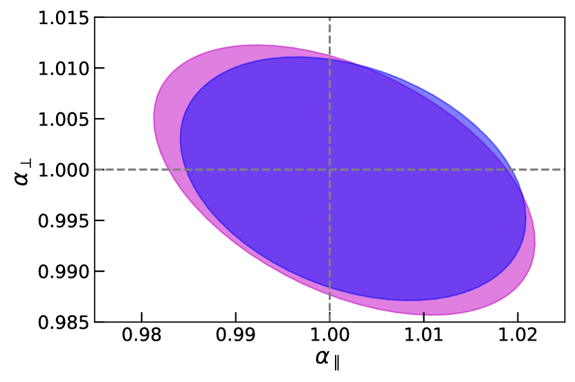
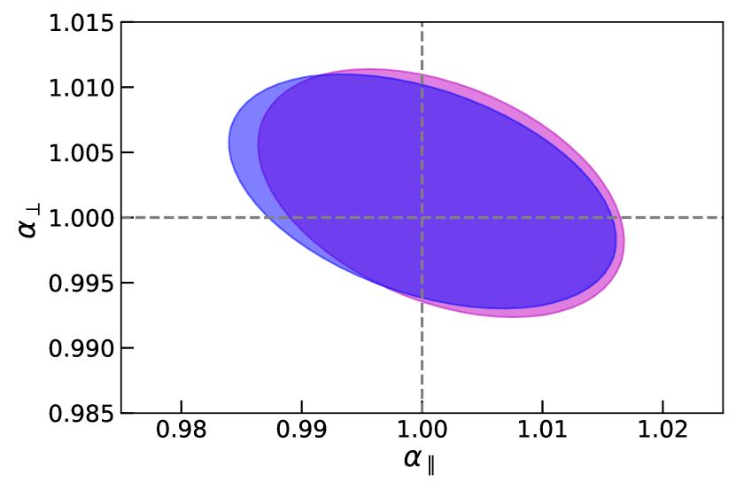
Figure 6: $\alpha_{\parallel}$ and $\alpha_{\perp}$ 1-$\sigma$ confidence interval for redshift space lower mass bin halo field at $z=0$ (top) and $z=1$ (bottom). Blue: HE18, magenta: ES3. We use scatter as the error and the values are present in Table 3. We calculate the covariance between the two parameters from 50 fits. The two contours show that HE18 and ES3 are consistent and the fitting results are also consistent with the fiducial cosmology.

In redshift space, the performance of HE18 and ES3 are again consistent. Both algorithms improve the error estimates by about a factor of 2-4. The improvement is slightly more significant at $z=0$ than at $z=1$. To show the size of the errors of the BAO parameter estimates after reconstruction, we present the confidence interval contours using the scatters of the estimates shown in Figure 6, for the lower mass halo field as an example. As shown in this figure, the estimated $\alpha_{\parallel}$ and $\alpha_{\perp}$ are consistent with the true values. In Table 3, we also present fitting results for another halo sample. We fix the halo number density at $3\times 10^{-4}$ $\rm{Mpc}^{3}$ at $z=0$ and 1; this way we can directly compare the results at the two redshift. The results again show slightly better performance at $z=0$. Both algorithms improve the error estimate of $\alpha_{\parallel}$ by about a factor of 2.2 at $z=0$ and 1, but improve by a factor of 3 for $\alpha_{\perp}$ at $z=0$ versus 2.2 at $z=1$, although the absolute errors are more often larger at $z=0$.

We also examine the cross-correlation between the measured $\alpha$ after reconstruction and the $\alpha$ of initial condition, using the 50 pairs of simulations, in Table 4. The smoothing scale presented is again 7.5 $h^{-1}\ \rm{Mpc}$. We find that HE18 are consistently more correlated with initial condition in both real and redshift space and across different fields. Moreover, often the smaller the smoothing scale, the better the cross-correlation, shown in Table 5 with real space matter field at $z=0$ as an example. The observation that an $\alpha$ cross-correlation for a higher smoothing scale for HE18 is matched with a smaller smoothing scale by ES3, if it can be matched, echos the trend in the propagator results. Within one reconstruction algorithm, the smaller the smoothing, the better the $\alpha$ cross-correlation suggests that larger smoothing could add additional noise to the distance measures. Recent studies (e.g. Chen et al., 2019) argue a larger smoothing for the ES3 algorithm, for a better match with theory. However, we do not detect any bias in our BAO fits using a relatively small smoothing. For HE18, since the smoothing starts at a large value ($R_{\rm ini}=20\ h^{-1}\ \rm{Mpc}$) and gradually reduces to its final value, it may be possible to push to smaller smoothing scales. Hybrid algorithms that pair reconstruction algorithms like HE18 and ES3 with machine learning Shallue & Eisenstein (2023); Chen et al. (2023) may also make the exact choice of smoothing scale less relevant. We leave a detailed study of these for later work.

field	redshift	sample	$\alpha$ mean	$\alpha$ scatter	$\alpha$ std
matter	0	pre-recon	1.0059	0.0138	0.0130
		HE18 (7.5)	1.0007	0.0038	0.0047
		ES3 (7.5)	1.0010	0.0044	0.0054
	1	pre-recon	1.0031	0.0072	0.0077
		HE18 (7.5)	1.0006	0.0037	0.0044
		ES3 (7.5)	1.0007	0.0039	0.0046
halo lower mass bin	0	pre-recon	1.0027	0.0152	0.0151
		HE18 (7.5)	0.9997	0.0085	0.0080
		ES3(7.5)	0.9997	0.0088	0.0086
	1	pre-recon	1.0041	0.0101	0.0105
		HE18 (7.5)	1.0013	0.0064	0.0067
		ES3 (7.5)	1.0016	0.0065	0.0070
halo higher mass bin	0	pre-recon	1.0107	0.0164	0.0168
		HE18 (7.5)	1.0034	0.0110	0.0095
		ES3 (7.5)	1.0037	0.0115	0.0105
	1	pre-recon	1.0053	0.0127	0.0125
		HE18 (7.5)	1.0003	0.0074	0.0085
		ES3 (7.5)	1.0006	0.0070	0.0088

Table 2: BAO parameter fits for matter and halo fields in real space for both reconstruction methods at $z=0$ and 1. The after reconstruction entries represent $\alpha$ constraints using smoothing scales 7.5 $h^{-1}\ \rm{Mpc}$ for both HE18 and ES3.

field	redshift	sample	$\alpha_{\parallel}$ mean	$\alpha_{\parallel}$ scatter	$\alpha_{\parallel}$ std	$\alpha_{\perp}$ mean	$\alpha_{\perp}$ scatter	$\alpha_{\perp}$ std
matter	0	pre-recon	1.0247	0.0423	0.0457	1.0019	0.0250	0.0211
		HE18 (7.5)	1.0028	0.0130	0.0121	1.0005	0.0055	0.0071
		ES3 (7.5)	1.0002	0.0142	0.0128	1.0009	0.0068	0.0080
	1	pre-recon	1.0173	0.0306	0.0326	0.9996	0.0149	0.0131
		HE18 (7.5)	1.0013	0.0119	0.0106	1.0005	0.0049	0.0066
		ES3 (7.5)	1.0015	0.0122	0.0117	1.0008	0.0054	0.0069
halo lower mass bin	0	pre-recon	1.0281	0.0461	0.0485	0.9967	0.0293	0.0248
		HE18 (7.5)	1.0025	0.0185	0.0183	0.9991	0.0118	0.0121
		ES3 (7.5)	1.0012	0.0199	0.0191	0.9992	0.0129	0.0126
	1	pre-recon	1.0181	0.0325	0.0376	1.0018	0.0197	0.0164
		HE18 (7.5)	1.0003	0.0159	0.0157	1.0018	0.0089	0.0100
		ES3 (7.5)	1.0017	0.0153	0.0164	1.0020	0.0093	0.0105
halo higher mass bin	0	pre-recon	1.0199	0.0428	0.0549	1.0112	0.0279	0.0283
		HE18 (7.5)	1.0064	0.0231	0.0223	1.0009	0.0144	0.0137
		ES3 (7.5)	1.0069	0.0259	0.0230	1.0011	0.0148	0.0150
	1	pre-recon	1.0256	0.0414	0.0435	0.9995	0.0228	0.0206
		HE18 (7.5)	1.0083	0.0235	0.0226	0.9978	0.0107	0.0128
		ES3 (7.5)	1.0073	0.0223	0.0203	0.9983	0.0103	0.0133
halo fixed number density	0	pre-recon	1.0254	0.0429	0.0516	1.0035	0.0282	0.0246
		HE18 (7.5)	1.0047	0.0198	0.0164	0.9998	0.0092	0.0107
		ES3 (7.5)	1.0028	0.0199	0.0185	1.0000	0.0100	0.0116
	1	pre-recon	1.0244	0.0398	0.0413	1.0002	0.0209	0.0182
		HE18 (7.5)	1.0062	0.0190	0.0191	1.0000	0.0094	0.0107
		ES3 (7.5)	1.0049	0.0173	0.0183	1.0005	0.0092	0.0108

Table 3: BAO parameter fits in redshift space for matter and halo fields at both redshift. After reconstruction values represent HE18 and ES3 both with 7.5 $h^{-1}\ \rm{Mpc}$ smoothing.

field	space	redshift	pre-recon	HE18	ES3
matter	real	0	0.3204	0.8595	0.8022
		1	0.5555	0.9012	0.8999
	redshift	0	0.3389	0.7738	0.6465
		1	0.5008	0.8799	0.8324
halo lower mass bin	real	0	0.3142	0.5009	0.4462
		1	0.4885	0.6865	0.6719
	redshift	0	0.3151	0.4616	0.3728
		1	0.4508	0.6782	0.6559
halo higher mass bin	real	0	0.4643	0.6121	0.6403
		1	0.2774	0.4603	0.4219
	redshift	0	0.4586	0.6358	0.6079
		1	0.3282	0.5139	0.4826
halo fixed number density	redshift	0	0.2104	0.4142	0.4307
		1	0.3752	0.5526	0.5979

Table 4: Cross-correlation of $\alpha$ post-reconstruction with the initial condition.

	15	10	7.5
HE18	0.5776	0.7288	0.7738
ES3	0.5016	0.6252	0.6465

Table 5: Cross-correlation between $\alpha$ after reconstruction and that from initial condition for matter field in redshift space at $z=0$.

6 Discussion

6.1 HE18 with ${\bf S}_{l}^{(2)}$ turned off

One of the major differences between HE18 and the ES3 method is whether the second order solution to the Euler-Poisson equation is used in the reconstruction procedure. When the second order correction is turned off in HE18, the theoretical assumptions are essentially the same for the two methods. Therefore, we can isolate this theoretical input and evaluate the contributions from other features in HE18, such as the iterative mechanism and annealing smoothing.

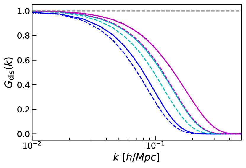
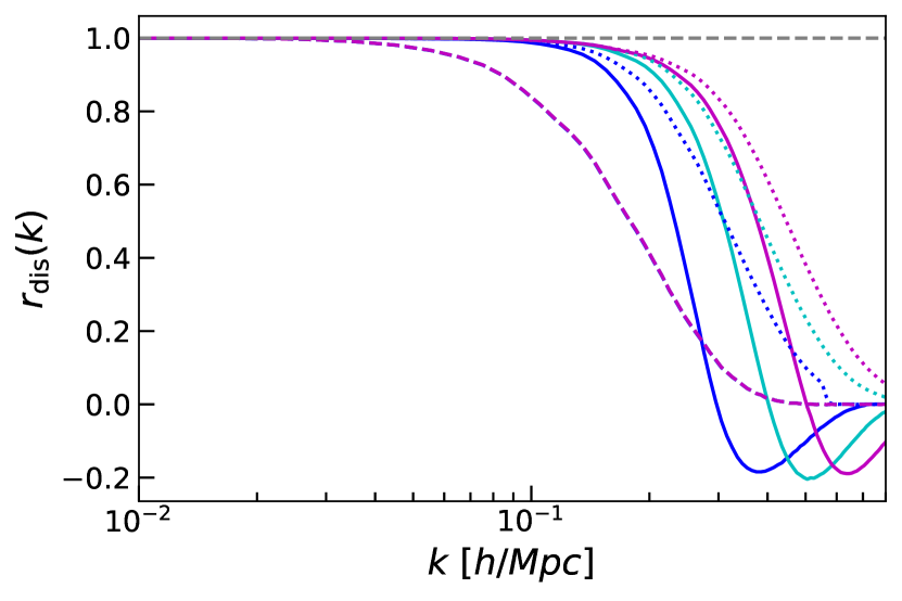
Figure 7: Displacement field cross-correlations by HE18 with $S^{(2)}$ turned on (solid) and off (dotted) and by ES3 (dashed) for the matter field in redshift space $z=0$. Both $S^{(2)}$ turned on and off for HE18 gives better results compared with ES3 for a given smoothing scale. However, results of a smaller smoothing by ES3 can be matched with a larger smoothing by HE18 in displacement propagator $G_{\rm dis}(k)$. In displacement propagator, the differences between $S^{(2)}$ turned on and off are negligible, but in displacement cross-correlation coefficient $r_{\rm dis}(k)$, the differences are more significant. Also, HE18 with $S^{(2)}$ turned off produces a better displacement cross-correlation. Different smoothing scales for ES3 does not make a difference in $r_{\rm dis}(k)$ because the smoothing kernel cancels out. Results of real space of matter field are similar.

Since the second-order perturbation equations are used to determine the displacements, we start by comparing the observed displacement to the actual particle displacements (the difference between final and initial positions). Analogous to the density field, we construct the propagator and cross-correlation coefficient of the displacement fields by

$$G_{\rm dis}(k)=\frac{\left<{\bf\tilde{S}}_{l}(k)\cdot{\bf\tilde{S}_{\rm true}^{*}(k)}\right>}{\left<|{\bf\tilde{S}_{\rm true}(k)}|^{2}\right>}$$ (33)

and

$$r_{\rm dis}(k)=\frac{\left<{\bf\tilde{S}}_{l}(k)\cdot{\bf\tilde{S}_{\rm true}^{*}(k)}\right>}{\sqrt{\left<|{\bf\tilde{S}}_{l}(k)|^{2}\right>\left<|{\bf\tilde{S}_{\rm true}(k)}|^{2}\right>}}$$ (34)

Figure 7 shows that the propagator in redshift space matter fields between ${\bf S}_{l}^{(s)}$ and ${\bf S}_{\rm true}$ and that between ${\bf S}_{l}^{(1)}$ and ${\bf S}_{\rm true}$ are virtually indistinguishable, while for $r(k)$, adding in the second-order solution appears to decorrelate the displacement field. By comparison, at the same smoothing scale, the ES3 method produces a displacement field that is noticeably worse than either variant of HE18. The discrepancy in $G(k)$ may be mitigated by working at a smaller smoothing scale, but this is not the case for $r(k)$, which is independent of the smoothing. We believe that this improvement comes from the fact that the HE18 algorithm estimates the density field in Lagrangian space (iteratively), and uses this density to estimate the displacement field. Since the input to our perturbation theory equations is the density field in Lagrangian space, this appears to be a more accurate approach.

Given the relatively small changes in the displacement field, it is not surprising that including/excluding the second-order terms make little difference in the final reconstructed field (in any of the metrics we have considered above). We therefore conclude that one can safely drop this correction in the algorithm with no degradation to the reconstruction. We also note that some previous studies that looked at second-order correction for reconstruction also find negligible differences (e.g. Seo et al., 2010; Schmittfull et al., 2017).

6.2 Annealing anisotropic smoothing in redshift space

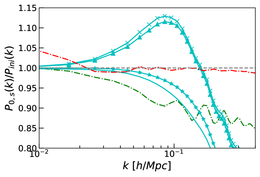
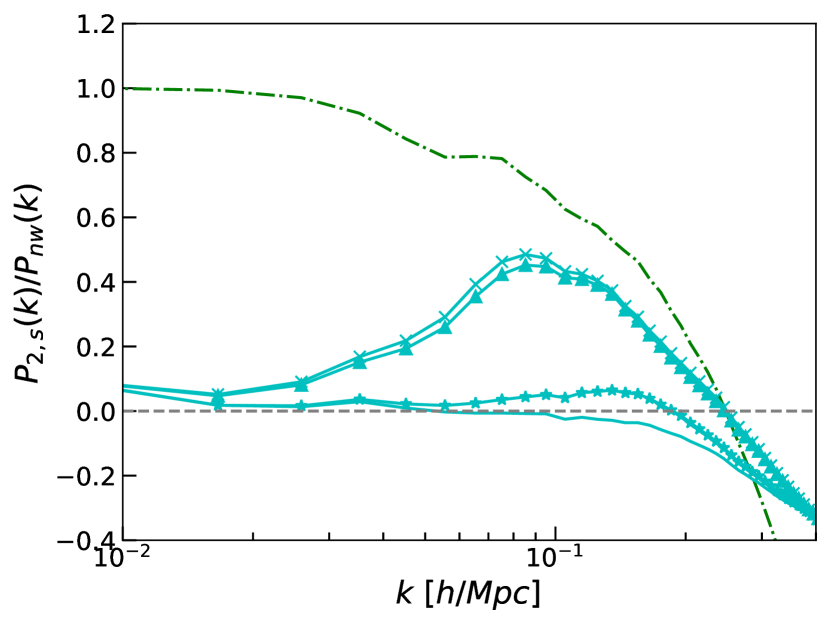
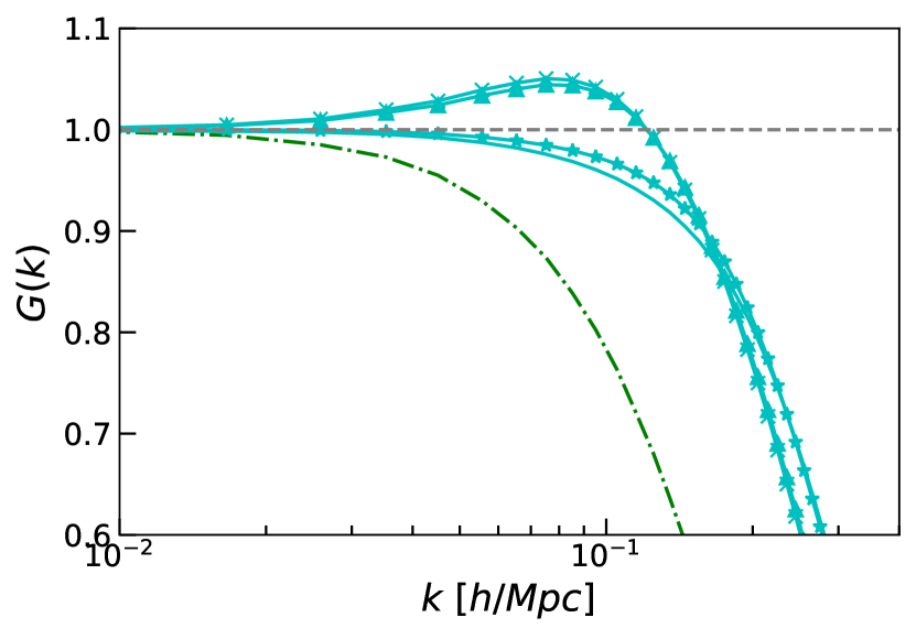
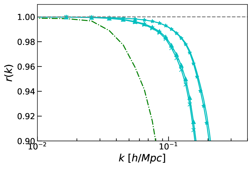
Figure 8: Monopole (upper left), quadrupole (upper right) power spectra, propagator (lower left) and cross-correlation coefficient (lower right) of annealing anisotropic smoothing for redshift space matter field using HE18 with 10 $h^{-1}\ \rm{Mpc}$ smoothing at $z=0$. Note that we divide the monopole power spectrum by the initial power spectrum, instead of no-wiggle power spectrum, to better show the pattern. Solid line is isotropic smoothing, crossed line is anisotropic smoothing with $C_{\rm ani}$=2.5 without annealing, and triangle and star lines are anisotropic smoothing with $C_{\rm ani,ini}$=2.5 with annealing rate equal to 1.01 and 1.1, respectively. Green dash-dotted line is before reconstruction. Red dash-dotted line is linear theory. In all but the cross-correlation coefficient, anisotropic smoothing with $C_{\rm ani,ini}$=2.5 and with a higher annealing rate (star line) gives the best results.

HE18 implemented the idea of using an anisotropic smoothing kernel in reconstruction. However, they kept the degree of anisotropy fixed over the course of the reconstruction. Since the intermediate steps in the reconstruction yield a density field with redshift space distortions reduced, it is interesting to ask whether reducing the degree of anisotropy with each iteration could improve the reconstruction. This is analogous to the annealing of the overall isotropic smoothing scale that works from the largest scales down to smaller scales. In order to implement this, we use a simple annealing schedule described in Sec. 2.2.1.

Figure 8 shows results using annealing rates of 1.1 and 1.01 with a starting anisotropic factor $C_{\rm ani,ini}$=2.5 and 10 $h^{-1}\ \rm{Mpc}$ smoothing perpendicular to line of sight with redshift space matter field at $z=0$. In both monopole and quadrupole power spectra and propagator, $C_{\rm ani}$=2.5 with an annealing rate of 1.1 offers better performance as measured in the propagator and power spectra, and a similar cross-correlation coefficient. In particular, the reduction in the anisotropic smoothing appears to be able to mitigate the RSD bump seen in the propagator. Using this annealing rate does not also degrade the errors on the BAO distance parameters. As with our previous results, this suggests that these variants of the algorithm might be unnecessary for BAO reconstruction, but could be useful for other applications.

6.3 Anisotropic reconstruction in redshift space

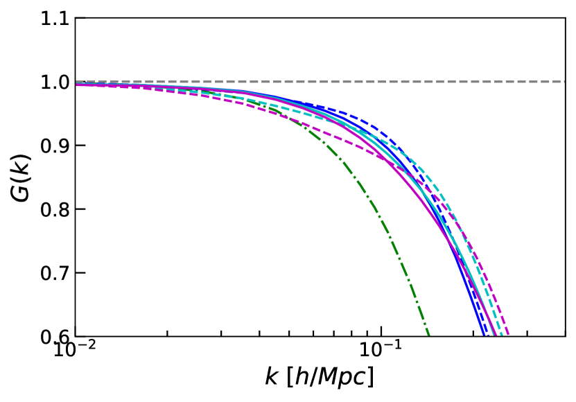
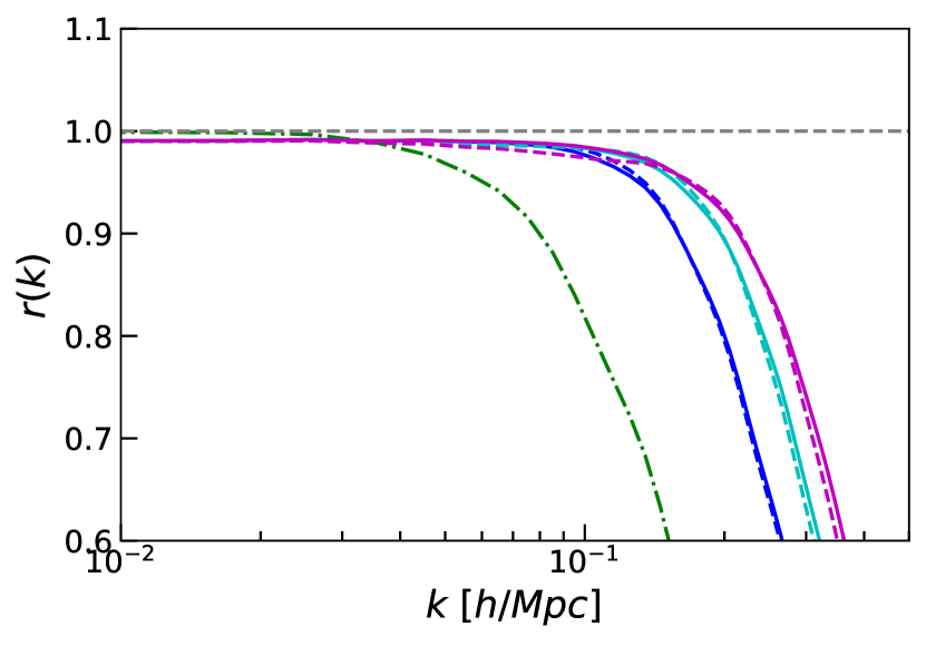
Figure 9: $G(k)$ and $r(k)$ of anisotropic reconstruction for matter field at $z=0$. Line styles and color scheme follow those in Figure 1. Different smoothing scales do not produce clear differences in the propagator, but do so in $r(k)$. The larger the smoothing scale, the faster it falls.

We examine the anisotropic reconstruction using matter field at $z=0$, leaving the RSD signal in the data. Figure 9 shows $G(k)$ and $r(k)$ with both algorithms and various smoothing scales. The RSD bump in the propagator is no longer present in these results, and we detect no clear trend with the smoothing scale, except that at the turnover, larger smoothing maintains slightly higher $G(k)$, although without a bump. This is roughly consistent with what we found in the isotropic case. The cross-correlation coefficient $r(k)$, however, does show a clear improvement with a decreasing smoothing scale, with very little difference between HE18 and ES3.

We also perform BAO fits with these reconstruction results. We use the same $\Sigma_{\perp}$ values as those used in isotropic reconstruction fits, but we set $\Sigma_{\parallel}=(1+f)\sigma_{\parallel}$, where $f$ is not reduced, after reconstruction. We also keep $R$-term at infinity. Comparing to isotropic reconstruction, the fits for $\alpha_{\parallel}$ are comparable to those isotropic counterparts. Both scatter and standard deviation of $\alpha_{\parallel}$ by HE18 are similar to those by ES3. Fits for $\alpha_{\perp}$ are also consistent with those in the corresponding isotropic cases. Also, the improvement after reconstruction is still larger at $z=0$ than at $z=1$, about a factor of 3.6 versus 2.6.

The advantages of leaving the RSD signal in the reconstructed data appear to be to reduce various artifacts from the smoothing scale, allowing better modeling of these results in the case of the ES3 algorithm. We currently do not have a full model for the HE18 reconstructed field and so it is not clear that the same modeling advantages transfer to this case, although eg. the mitigation of the feature in the propagator is suggestive. However, since many of these are broadband features, they do not significantly impact the BAO fits.

6.4 HE18 vs ES3

Our primary conclusion from this study is that the HE18 and ES3 methods are generally quite comparable in terms of performance across metrics that focus both on the density field as well as fitting the BAO feature. We find that the ES3 method can return similar results in the cross-correlation coefficients and propagators to HE18, albeit using a smaller effective smoothing scale However, the HE18 method is more robust to the choice of smoothing scale, and so, has the potential to push down to smaller scales. The HE18 method does better at estimating the displacement field, and so, can better remove the RSD signal in the data. It also appears to do better at reconstructing the full broadband shape of the power spectrum, making it more useful for general LSS studies.

The two reconstruction methods show comparable results in BAO distance fitting in both real and redshift space. If we correlate the $\alpha$ values post-reconstruction with those measured from the initial density field, we find that HE18 does have a higher cross-correlation coefficient than ES3. This is consistent with the field-level $r(k)$ results above.

We find that HE18 is robust to the various parameter choices, and tracer populations. There are certain aspects where HE18 performs better than ES3; in particular, HE18 is significantly better at estimating the large scale velocity field and removing RSD. Even though HE18 does not present a substantial improvement in BAO fitting, it is a promising method to be applied in other areas of large-scale structure analysis.

7 Conclusions

We closely study the new iterative reconstruction algorithm by Hada & Eisenstein (2018) in comparison to the standard algorithm by Eisenstein et al. (2007a) with extensive analysis with two-point statistics and BAO fitting. Our findings are

• The two algorithms are largely comparable in two-point statistics, which include propagator and cross-correlation coefficient.

• HE18 is significantly better at removing RSD than ES3, as shown in quadrupole power spectrum.

• Fine tuning smoothing along line-of-sight can lead to reconstruction results slightly closer to the initial condition. However, the contribution of this to BAO fits is negligible.

• The two algorithms also produce consistent BAO distance fits.

• BAO fitting is robust against the difference in the reconstructed power spectrum produced by different algorithms and reconstruction convention (isotropic vs anisotropic reconstruction).

• The most important input to BAO fitting is the smoothing scale.

• Adding the second order perturbation theory has a negligible effect to reconstruction.

Although the two methods are largely consistent in various aspects, the HE18 algorithm remains an excellent reconstruction method to be employed in the ongoing and future large-scale structure surveys. Even though the difference is minimal in BAO fitting, HE18 algorithm may potentially have more significant benefits in other areas of analysis, for example, the full-shape analysis to constrain $f\sigma_{8}$, for its much better ability in removing RSDs.

While the scope of this work did not include extending the HE18 method to be applied on data with incomplete sky coverage and varying selection functions, we observe that these extensions should be relatively straightforward. In particular, solving for the displacement field is identical to the standard reconstruction method when the second order solution is not included. Therefore, much of the same methodology (e.g. Padmanabhan et al., 2012; Burden et al., 2015) developed for the ES3 method can be directly applied here. Furthermore, since the HE18 method keeps track of the overall density field, it would be possible to track where the boundary pixels are advected to, and iteratively refine the exact volume of the survey. We defer a detailed implementation of these ideas to future work.

Data Availability

The Python implementations of both the HE18 and ES3 algorithms, two-point statistics calculations, and BAO fitting codes developed in this work are publicly available at https://github.com/xinyidotchen/reconstruction and https://github.com/xinyidotchen/BAOfitting. The statistics produced in the analysis are available upon request. The Quijote simulations used in this work are publicly available with details in (Villaescusa-Navarro et al., 2019).

References

- Aghanim et al. (2020) Aghanim N., et al., 2020, Astronomy & Astrophysics, 641, A6
- Alam et al. (2017) Alam S., et al., 2017, Monthly Notices of the Royal Astronomical Society, 470, 2617
- Anderson et al. (2012) Anderson L., et al., 2012, Monthly Notices of the Royal Astronomical Society, 427, 3435
- Anderson et al. (2014a) Anderson L., et al., 2014a, Monthly Notices of the Royal Astronomical Society, 439, 83
- Anderson et al. (2014b) Anderson L., et al., 2014b, MNRAS, 441, 24
- Beutler et al. (2015) Beutler F., Blake C., Koda J., Marín F. A., Seo H.-J., Cuesta A. J., Schneider D. P., 2015, Monthly Notices of the Royal Astronomical Society, 455, 3230
- Beutler et al. (2016) Beutler F., et al., 2016, Monthly Notices of the Royal Astronomical Society, 464, 3409
- Buchert (1994) Buchert T., 1994, MNRAS, 267, 811
- Buchert & Ehlers (1993) Buchert T., Ehlers J., 1993, MNRAS, 264, 375
- Burden et al. (2015) Burden A., Percival W. J., Howlett C., 2015, MNRAS, 453, 456
- Chen et al. (2019) Chen S.-F., Vlah Z., White M., 2019, J. Cosmology Astropart. Phys., 2019, 017
- Chen et al. (2023) Chen X., Zhu F., Gaines S., Padmanabhan N., 2023, MNRAS, 523, 6272
- Chudaykin & Ivanov (2019) Chudaykin A., Ivanov M. M., 2019, J. Cosmology Astropart. Phys., 2019, 034
- DESI Collaboration et al. (2016) DESI Collaboration et al., 2016, The DESI Experiment Part I: Science,Targeting, and Survey Design (arXiv:1611.00036)
- Duan & Eisenstein (2019) Duan Y., Eisenstein D., 2019, MNRAS, 490, 2718
- Eisenstein & Hu (1998) Eisenstein D. J., Hu W., 1998, ApJ, 496, 605
- Eisenstein et al. (2007a) Eisenstein D. J., Seo H.-J., Sirko E., Spergel D. N., 2007a, ApJ, 664, 675
- Eisenstein et al. (2007b) Eisenstein D. J., Seo H., White M., 2007b, The Astrophysical Journal, 664, 660
- Gil-Marín et al. (2020) Gil-Marín H., et al., 2020, MNRAS, 498, 2492
- Hada & Eisenstein (2018) Hada R., Eisenstein D. J., 2018, MNRAS, 478, 1866
- Kaiser (1987) Kaiser N., 1987, MNRAS, 227, 1
- Kazin et al. (2014) Kazin E. A., et al., 2014, Monthly Notices of the Royal Astronomical Society, 441, 3524
- LSST Science Collaboration et al. (2009) LSST Science Collaboration et al., 2009, LSST Science Book, Version 2.0 (arXiv:0912.0201)
- Laureijs et al. (2011) Laureijs R., et al., 2011, Euclid Definition Study Report (arXiv:1110.3193)
- Mehta et al. (2011) Mehta K. T., Seo H.-J., Eckel J., Eisenstein D. J., Metchnik M., Pinto P., Xu X., 2011, ApJ, 734, 94
- Meiksin et al. (1999) Meiksin A., White M., Peacock J. A., 1999, MNRAS, 304, 851
- Noh et al. (2009) Noh Y., White M., Padmanabhan N., 2009, Phys. Rev. D, 80, 123501
- Obuljen et al. (2017) Obuljen A., Villaescusa-Navarro F., Castorina E., Viel M., 2017, Journal of Cosmology and Astro-Particle Physics, 2017, 012
- Padmanabhan & White (2008) Padmanabhan N., White M., 2008, Phys. Rev. D, 77, 123540
- Padmanabhan & White (2009) Padmanabhan N., White M., 2009, Physical Review D, 80
- Padmanabhan et al. (2009) Padmanabhan N., White M., Cohn J. D., 2009, Phys. Rev. D, 79, 063523
- Padmanabhan et al. (2012) Padmanabhan N., Xu X., Eisenstein D. J., Scalzo R., Cuesta A. J., Mehta K. T., Kazin E., 2012, MNRAS, 427, 2132
- Park et al. (1994) Park C., Vogeley M. S., Geller M. J., Huchra J. P., 1994, ApJ, 431, 569
- Peacock & Dodds (1994) Peacock J. A., Dodds S. J., 1994, MNRAS, 267, 1020
- Ross et al. (2015) Ross A. J., Samushia L., Howlett C., Percival W. J., Burden A., Manera M., 2015, Monthly Notices of the Royal Astronomical Society, 449, 835
- Schmittfull et al. (2015) Schmittfull M., Feng Y., Beutler F., Sherwin B., Chu M. Y., 2015, Phys. Rev. D, 92, 123522
- Schmittfull et al. (2017) Schmittfull M., Baldauf T., Zaldarriaga M., 2017, Phys. Rev. D, 96, 023505
- Seo & Eisenstein (2005) Seo H.-J., Eisenstein D. J., 2005, ApJ, 633, 575
- Seo & Eisenstein (2007) Seo H.-J., Eisenstein D. J., 2007, ApJ, 665, 14
- Seo & Hirata (2016) Seo H.-J., Hirata C. M., 2016, Monthly Notices of the Royal Astronomical Society, 456, 3142
- Seo et al. (2010) Seo H.-J., et al., 2010, The Astrophysical Journal, 720, 1650
- Seo et al. (2016) Seo H.-J., Beutler F., Ross A. J., Saito S., 2016, Monthly Notices of the Royal Astronomical Society, 460, 2453
- Seo et al. (2021) Seo H.-J., Ota A., Schmittfull M., Saito S., Beutler F., 2021, Iterative reconstruction excursions for Baryon Acoustic Oscillations and beyond (arXiv:2106.00530)
- Shallue & Eisenstein (2023) Shallue C. J., Eisenstein D. J., 2023, MNRAS, 520, 6256
- Spergel et al. (2013) Spergel D., et al., 2013, arXiv e-prints, p. arXiv:1305.5422
- Tassev & Zaldarriaga (2012) Tassev S., Zaldarriaga M., 2012, Journal of Cosmology and Astroparticle Physics, 2012, 006
- Villaescusa-Navarro et al. (2019) Villaescusa-Navarro F., et al., 2019, The Quijote simulations (arXiv:1909.05273)
- White (2014) White M., 2014, Monthly Notices of the Royal Astronomical Society, 439, 3630
- Xu et al. (2012) Xu X., Padmanabhan N., Eisenstein D. J., Mehta K. T., Cuesta A. J., 2012, Monthly Notices of the Royal Astronomical Society, 427, 2146
- Xu et al. (2013) Xu X., Cuesta A. J., Padmanabhan N., Eisenstein D. J., McBride C. K., 2013, MNRAS, 431, 2834
- Zel’Dovich (1970) Zel’Dovich Y. B., 1970, A&A, 500, 13