Mori–Zwanzig Modal Decomposition

Abstract

We introduce the Mori-Zwanzig (MZ) Modal Decomposition (MZMD), a novel technique for performing modal analysis of large scale spatio-temporal structures in complex dynamical systems, and show that it represents an efficient generalization of Dynamic Mode Decomposition (DMD). The MZ formalism provides a mathematical framework for constructing non-Markovian reduced-order models of resolved variables from high-dimensional dynamical systems, incorporating the effects of unresolved dynamics through the memory kernel and orthogonal dynamics. We present a formulation and analysis of the modes and spectrum from MZMD and compare it to DMD when applied to a complex flow: a Direct Numerical Simulation (DNS) data-set of laminar-turbulent boundary-layer transition flow over a flared cone at Mach 6. We show that the addition of memory terms by MZMD improves the resolution of spatio-temporal structures within the transitional/turbulent regime, which contains features that arise due to nonlinear mechanisms, such as the generation of the so-called "hot" streaks on the surface of the flared cone. As a result, compared to DMD, MZMD improves future state prediction accuracy, while requiring nearly the same computational cost.

1 Introduction

Transitional and turbulent flows arise in many applications, and often contain a wide range of coherent structures; the analysis of which are key in understanding the dominant physical mechanisms present in the flow. Typical techniques involve modal decompositions of an experimental or numerical data-set of the flow field (Taira et al., 2017). For example, extracting the most energetic spatial modes with proper orthogonal decomposition (POD) (Holmes & Lumley, 2012), or the spatio-temporal coherent structures with Dynamic Mode Decomposition (DMD) (Schmid, 2010) and Spectral POD (Towne et al., 2018).

For compressible viscous flows, the classical POD–Galerkin method has challenges due to discontinuities that might be generated by the underlying equations and unstable temporal coefficients (Kalashnikova et al., 2014; Gloerfelt, 2008). DMD, being fully data-driven, avoids some of these issues for compressible flows, making it an attractive approach. DMD has been applied in the context of supersonic and hypersonic flows, such as developing reduced models (Yu et al., 2019) and modal analysis of DNS data for understanding the underlying transition mechanisms (Subbareddy et al., 2014).

Although DMD has connections to the Koopman operator (Rowley et al., 2009), in practice finding a Koopman invariant subspace can be intractable. DMD also has limitations with extracting nonlinear mechanisms and intermediate transients (Wu et al., 2021). Therefore, in this work, we explore the data-driven Mori-Zwanzig (MZ) approach first derived in Lin et al. (2021) and further extended in Lin et al. (2022), which generalizes the approximate Koopmanian learning and has shown to improve the prediction performance over Extended DMD (EDMD) (Williams et al., 2015). We construct a novel MZ modal decomposition technique which includes memory without the more costly time-delay embeddings (Kamb et al., 2020; Arbabi & Mezić, 2017) or Higher-Order DMD (Le Clainche & Vega, 2017).

The MZ formalism, originally developed in statistical mechanics (Mori, 1965; Zwanzig, 1973), provides a mathematical framework for constructing non-Markovian reduced-order models of a reduced set of observables from high-dimensional dynamical systems, where the effects due to the unresolved dynamics are captured in the memory kernel and orthogonal dynamics (Lin et al., 2021). The resulting formulation, referred to as the Generalized Langevin equation (GLE), consists of a Markovian term, a memory term, and a orthogonal dynamics term. The memory term quantifies the interactions between the resolved and under-resolved dynamics, and is related to the orthogonal dynamics term through the fluctuation-dissipation theorem. Up until recently, modeling turbulence with the MZ formalism has been extremely challenging due to the unknown structure of the memory kernel, which is affected by the unresolved orthogonal dynamics (Tian et al., 2021b; Parish & Duraisamy, 2017). However, with the recent progress (Lin et al., 2021, 2022), the MZ operators have been learned in turbulent (Tian et al., 2021a) and transitional flows (Woodward et al., 2023b, c). Here, we extend the formulation as a modal decomposition technique.

This manuscript is organized as follows. Sec. 2 summarizes the data-driven MZ method developed in Lin et al. (2021). Sec. 3 describes the low-rank approximation of the MZ operators with a POD based projection, and proves that the modes of the low-rank GLE approximate the modes of the full GLE. Sec. 5 compares the MZMD and DMD approaches for wall pressure disturbance data obtained from a "natural" transition simulation for a flared cone at Mach 6 (Hader & Fasel, 2018). Sec. 6 provides concluding remarks.

2 Data-Driven Mori–Zwanzig

Following Lin et al. (2021, 2022), we consider the discrete-time autonomous deterministic dynamical system where the states $\bm{x}(t)\in\mathbb{R}^{D}$ evolve according to

$$\bm{x}_{n+1}=\bm{F}(\bm{x}_{n}),\quad\bm{x}(0)=\bm{x}_{0},$$ (1)

where $\bm{F}:\mathbb{R}^{D}\rightarrow\mathbb{R}^{D}$ is the flow map and $n$ denotes the discrete time step. The discrete-time formulation is a natural start when considering simulation or experimental data. Next, we seek evolutionary equations for a set of observables $\bm{g}\in\mathbb{R}^{r},r\leq D$, with $g_{i}:\mathbb{R}^{D}\rightarrow\mathbb{R}$, $i=1,...,r$. The observables are, in general, functions of the states $\bm{x}$. In this study, the observables are selected using an SVD-based compression of the pressure field at the surface of the flared cone. The central result of the MZ procedure is the GLE (see Mori (1965); Zwanzig (1973); Lin et al. (2021) for detailed derivations), which prescribes the exact and closed set of evolutionary equations for the observables given any initial condition $\bm{x}_{0}$ as:

$$\bm{g}_{n+1}(\bm{x}_{0})=\bm{\mathit{\Omega}}_{0}(\bm{g}_{n}(\bm{x}_{0}))+\sum_{l=1}^{n}\bm{\mathit{\Omega}}_{l}(\bm{g}_{n-l}(\bm{x}_{0}))+\bm{W}_{n}(\bm{x}_{0}),$$ (2)

where $\bm{g}_{n}:\mathbb{R}^{D}\rightarrow\mathbb{R}^{r}$ is the $r\times 1$ vector of functions of the initial state $\bm{x}_{0}$ so that $\bm{g}_{n}(\bm{x}_{0})\equiv\bm{g}(\bm{x}(n\Delta t;\bm{x}_{0}))\equiv\bm{g}(\bm{F}^{n}(\bm{x}_{0}))$. The GLE (Eq. 2) states that the vector of observables at time $n+1$ evolves (and is decomposed) according to three parts: (1) a Markovian operator: $\bm{\mathit{\Omega}}_{0}:\mathbb{R}^{r}\rightarrow\mathbb{R}^{r}$ which only depends on the observables at the previous time step ($n$), (2) the memory kernel: the series of operators $\bm{\mathit{\Omega}}_{l}:\mathbb{R}^{r}\rightarrow\mathbb{R}^{r}$ depending on observables with a time lag $l$, and (3) the orthogonal dynamics: $\bm{W}_{n}:\mathbb{R}^{D}\rightarrow\mathbb{R}^{r}$ depending on the full initial state $\bm{x}_{0}$. The above GLE is general for any projection operator (see Lin et al. (2022) for a detailed discussion). Using Mori’s linear projection (Mori, 1965), which employs the equipped inner product in the $L^{2}$ Hilbert space to define the functional projection, results in a linear Markovian form $\bm{\mathit{\Omega}}_{0}(\bm{g}_{n}(\bm{x}_{0}))={\bm{\Omega}}_{0}\cdot\bm{g}_{n}(\bm{x}_{0})$, and linear memory kernel $\bm{\mathit{\Omega}}_{l}(\bm{g}_{n-l}(\bm{x}_{0}))={\bm{\Omega}}_{l}\cdot\bm{g}_{n-l}(\bm{x}_{0})$, where ${\bm{\Omega}}_{l}$’s are $r\times r$ matrices. In this manuscript, we assume that, in the process of learning the MZ operators with the convex optimization scheme derived in Lin et al. (2021), $\bm{W}_{n}$ is a small and negligible residual term. The algorithms for extracting the memory kernel is described in Appendix for completeness.

3 Mori–Zwanzig Modal Decomposition

Building upon this data-driven MZ approach, we construct a novel modal analysis technique which includes memory effects without the more costly time-delay embeddings (Kamb et al., 2020). Similar to DMD, we use SVD compression to provide a tractable method for extracting the modes and spectrum in the state space from a reduced set of observables defined using POD modes. Rather than starting with standard DMD assumption that the evolution of state variables is linear (i.e., $\bm{x}_{n+1}=\bm{A}\bm{x}_{n}$), with MZMD, we start from the discrete-time GLE (2) and assume that the higher-order orthogonal dynamics are negligible. This is formalized with the Mori’s projector and $D$ state observables selected as $\pi_{i}\triangleq\pi_{i}\left(\mathbf{x}\right)=x_{i}$. Assuming that only $k$ memory terms are sufficient so that the higher-order orthogonal dynamics are negligible, Eq. (2) becomes

$$\bm{x}_{n+1}=\mathbf{\Omega}_{0}^{(x)}\cdot\bm{x}_{n}+...+\mathbf{\Omega}_{k}^{(x)}\cdot\bm{x}_{n-k},$$ (3)

where the linear MZ operators $\mathbf{\Omega}_{i}^{(x)}$ are acting in state space.

Now, decomposing the snapshot matrix using an SVD, $\bm{X}=[\bm{x}_{0},...,\bm{x}_{\tau}]\approx\bm{U}_{r}\bm{\Sigma}_{r}\bm{V}_{r}^{*}$, the reduced observables are selected as $\bm{g}(\bm{x}_{n})\triangleq\bm{U}_{r}^{*}\cdot\bm{x}_{n}$. Therefore, we can write Eq. 3 as

$$\bm{g}_{n+1}=\bm{\Omega}_{0}^{(g)}\cdot\bm{g}_{n}+...+\bm{\Omega}_{k}^{(g)}\cdot\bm{g}_{n-k},$$ (4)

where $\bm{\Omega}_{i}^{(g)}=\bm{U}_{r}^{*}\mathbf{\Omega}_{i}^{(x)}\bm{U}_{r}$ is the memory kernel $\mathbf{\Omega}_{i}^{(x)}$ projected onto the POD modes. We establish the relationship between the modes of 3 and 4 in two parts; first a full SVD ($r=D$) is used to establish the equivalence, then a truncated SVD is used ($r<D$) resulting in approximations of the modes of the full state GLE. We note that by adding memory kernels there is now a multiplicative interaction between the $\bm{\Omega}_{i}$’s, as seen in the long time dynamics described below. Furthermore, the modal analysis can be obtained through the associated block companion matrices

$$\bm{C}_{x}=\begin{bmatrix}\bm{\Omega}_{0}^{(x)}&\bm{\Omega}_{1}^{(x)}&...&\bm{\Omega}_{k}^{(x)}\\ \bm{I}&\bm{0}&...&\bm{0}\\ &\ddots&&\\ \bm{0}&...&\bm{I}&\bm{0}\\ \end{bmatrix}\quad\text{and}\quad\bm{C}_{g}=\begin{bmatrix}\bm{\Omega}_{0}^{(g)}&\bm{\Omega}_{1}^{(g)}&...&\bm{\Omega}_{k}^{(g)}\\ \bm{I}&\bm{0}&...&\bm{0}\\ &\ddots&&\\ \bm{0}&...&\bm{I}&\bm{0}\\ \end{bmatrix},$$ (5)

where $\bm{I}$ and $\bm{0}$ are the appropriately sized identity and zero matrices respectively. This shares a similar structure to Higher-Order DMD (Le Clainche & Vega, 2017), however, in this work the higher order terms $\bm{\Omega}^{(g)}_{k>0}$ are part of the MZ memory kernel, which satisfies the generalized fluctuation-dissipation relationship; each learned using the algorithms in Lin et al. (2021).

The solutions to Eq. 3 are therefore given by $\bm{x}_{n}=\bm{P}_{0}\bm{C}_{x}^{n}\bm{z}_{0}$, where $\bm{z}_{0}=[\bm{x}_{0},...,\bm{x}_{-k}]^{T}$ and $\bm{P}_{0}=[\bm{I}\hskip 2.84526pt\bm{0}\hskip 2.84526pt...\hskip 2.84526pt\bm{0}]$, and the solution for Eq. 4, is $\bm{g}_{n}=\bm{P}_{0}\bm{C}_{g}^{n}\tilde{\bm{z}}_{0}$ where $\tilde{\bm{z}}_{0}=[\bm{g}_{0},...,\bm{g}_{-k}]^{T}$. Thus, the solutions are fully characterized by the eigenpairs of the associated companion matrices. The eigenvectors identify the large-scale coherent structures and their associated eigenvalues determine the temporal evolution as seen in the basis expansion about the eigenvectors (modes) $\bm{\phi}_{i}$; $\bm{x}_{n}=\bm{P}_{0}\sum_{i}a_{i}\lambda_{i}^{n}\bm{\phi}_{i}=\sum_{i}a_{i}\lambda_{i}^{n}\bm{\phi}^{0}_{i}$, where $\bm{\phi}^{0}\equiv\bm{P}_{0}\bm{\phi}$. Next we show that the relationship between the eigenpair of the full system Eq. 3 with that of $\bm{C}_{g}$.

Theorem 1.

Let $(\lambda,\bm{w})$ be an eigenpair of $\bm{C}_{g}$ with $(r=D)$. Then $(\lambda,\bm{\phi})$ is and eigenpair of $\bm{C}_{x}$ where $\bm{\phi}=[\bm{\phi}^{0},(1/\lambda)\bm{\phi}^{0},...,(1/\lambda^{k})\bm{\phi}^{0}]^{T}$, and $\bm{\phi}^{0}=\bm{U}\bm{w}^{0}$.

Proof.

Let $\bm{X}=\bm{U}\bm{\Sigma}\bm{V}^{*}$ be the full SVD of the snapshot matrix ($r=D$). Then, expanding $\bm{C}_{g}\bm{w}=\lambda\bm{w}$, the associated nonlinear eigenvalue problem (Bai et al. (2000)) of $\bm{C}_{g}$ satisfies

$$\bm{\Omega}_{k}^{(g)}\bm{w}^{0}+\lambda\bm{\Omega}_{k-1}^{(g)}\bm{w}^{0}+...+\lambda^{k}\bm{\Omega}_{0}^{(g)}\bm{w}^{0}=\lambda^{k+1}\bm{w}^{0}.$$

Substituting $\bm{\Omega}_{i}^{(g)}=\bm{U}^{*}\mathbf{\Omega}_{i}^{(x)}\bm{U}$ then left multiplication by $\bm{U}$ results in

$$\bm{\Omega}_{k}^{(x)}(\bm{U}\bm{w}^{0})+\lambda\bm{\Omega}_{k-1}^{(x)}(\bm{U}\bm{w}^{0})+...+\lambda^{k}\bm{\Omega}_{0}^{(x)}(\bm{U}\bm{w}^{0})=\lambda^{k+1}(\bm{U}\bm{w}^{0}).$$

This is the associated nonlinear eigenvalue problem of $\bm{C}_{x}$, thus $(\lambda,\bm{\phi})$ is an eigenpair of $\bm{C}_{x}$. ∎

In practice, a truncated SVD is computed ($r<D$) to obtain a suitable low rank approximation. In this case, $\bm{U}_{r}\bm{U}_{r}^{*}$ forms an orthogonal projection operator, projecting onto the first $r$ POD modes of the snapshot matrix. This fact together with Theorem 1 allows us to approximate the modes and spectrum of the state space GLE 3 from the eigenpair of the reduced observable GLE 4, which is otherwise intractable for large systems. Figure 1 illustrates the relationships between observables, eigenpairs, and operators in these two spaces. The MZMD modes are consequently $\bm{\Phi}\equiv[\bm{\phi}_{1}^{0},...,\bm{\phi}_{rk}^{0}]$ and coefficients are then $\bm{a}=\tilde{\bm{\Phi}}^{\dagger}\bm{z}_{0}\approx(\bm{W})^{-1}\tilde{\bm{z}}_{0}$, where $\tilde{\bm{\Phi}}\equiv[\bm{\phi}_{1},...,\bm{\phi}_{rk}]$, and $\bm{W}$ the is eigenvector matrix of $\bm{C}_{g}$. This provides a scalable modal analysis technique that improves upon DMD by adding hysteresis effects with the Mori-Zwanzig formalism. It is useful to point out that when there is no memory present in MZMD, it is equivalent to DMD. Indeed, it has been established that MZ without memory terms is equivalent to EDMD (Lin et al., 2021). Thus, MZMD generalizes DMD using the MZ formalism to include memory effects within the modes and spectrum.

Figure 1: Diagram of the MZMD concept

4 Hypersonic Boundary Layer Transition

High-speed laminar–turbulent boundary-layer transition is a complex dynamical phenomenon and remains an active research area. Understanding high-speed boundary-layer transition is necessary in order to develop reliable transition prediction and flow control methods. This is important for the next-generation design and safe operation of advanced high-speed vehicles. Transition to turbulence leads to significant increases in skin friction (drag) and heat transfer, far exceeding the laminar values. Wind tunnel experiments (Chynoweth et al., 2019) as well as DNS (Hader & Fasel, 2019) showed the development of so-called “hot streaks” in the nonlinear transition regime that can locally significantly exceed the turbulent heat transfer values. Therefore, understanding the dominant physical mechanisms leading to laminar-turbulent boundary-layer transition is vital for the design stages of a high-speed vehicle. The transition process is inherently nonlinear and retains the memory of the inflow conditions. Therefore, reduced-order modeling can significantly aid in the understanding of the dominant nonlinear transition mechanisms.

In this work, we compare MZMD and DMD applied to a DNS data set of hypersonic boundary layer transition on a flared cone at Mach 6, where transition was initiated by random perturbations at the inflow of the computational domain (“natural” transition see Hader & Fasel (2018), schematically shown in Figure 2(a)). The "natural" transition DNS includes the relevant transition stages defined by Morkovin et al. (1994) from the primary instability all the way to breakdown to turbulence (see Figure 2(b)). The dataset used in this work is the statistically stationary 2D pressure field at the surface of the cone with $258\times 4600$ spatial resolution obtained from a full 3D DNS from Hader & Fasel (2019). The pressure at the wall is used as it contains dynamics relevant in the nonlinear generation of the so-called “hot streaks” seen in Figure 2(c). A training set of 6,000 snapshots in time is used for the MZMD and DMD procedures. This is the timescale in which the flow advects $\mathcal{O}(5L)$ where $L$ is the length of the computational domain. A held-out test set of 400 snapshots (where flow advects $\mathcal{O}(1/3L)$, or roughly 100 times the Kolmogorov timescale) are used for measuring generalization errors of future state prediction.

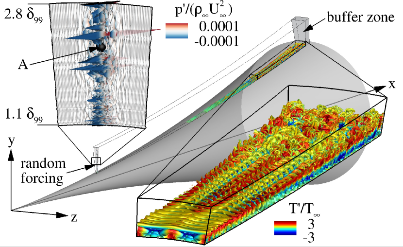
(a)

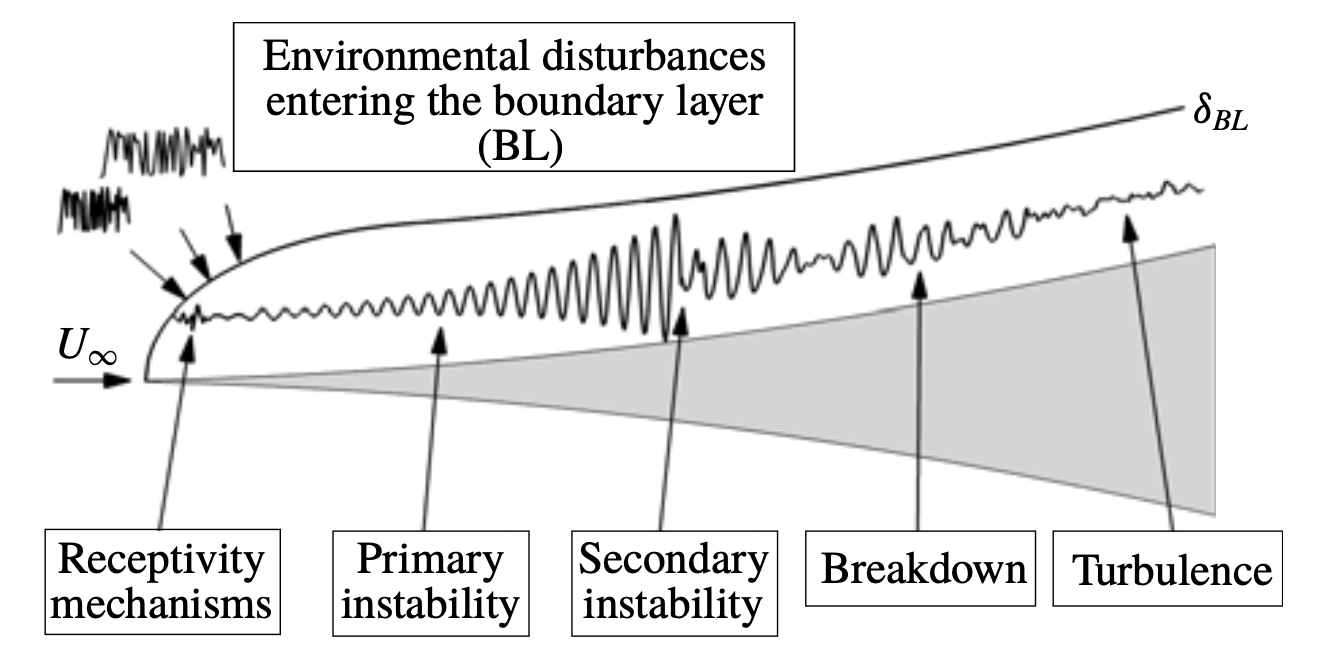
(b)

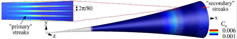
(c)

Figure 2: (2(a)) Computational setup for the "natural" transition DNS (Hader & Fasel, 2018), (2(b)) schematic of the transition stages Morkovin et al. (1994), and (2(c)) time-averaged Stanton number contours on the surface of the cone obtained from DNS.

5 Results

First, the rank $r$ is set in order to contain 98% of the variance in $\bm{X}$, which requires $r=410$ as seen in Fig. 3. This also demonstrates that $\bm{X}$ contains a sufficient amount of low-rank structure. In Fig. 3 we report the generalization errors of MZMD future state predictions on the test set with varying $k$ memory terms (see 3) as compared to DMD; this shows that $k=6$ is a sufficient number of memory terms to use, as the generalization errors converge. With $k=6$, we see the MZMD future state prediction provides a significant relative improvement in accuracy over DMD future state prediction.

The eigenvalues and amplitudes of MZMD and DMD modes are compared in Fig. 4. Two crucial differences emerge in this result. First, the ability to capture intermediate transient dynamics with MZMD as seen by the eigenvalues contained within the unit circle, which are associated with decaying transient modes from MZ memory effects. Second, the increase in the amplitudes of the modes associated with the second and third higher harmonics. The dominant modes of MZMD and DMD associated with the frequency of the dominant primary instability ($f\approx 300$ kHz) and the first and second higher harmonics, are shown in Figs. 5 and 6. From this we see that the modes from MZMD, as compared to DMD, are more focused within the transition region, especially at the location of the primary streaks (region where the strong modulation in the azimuthal direction is observed in Figs. 5 and 6). Furthermore, the fundamental mode of MZMD exhibits linear growth of axisymmetric structures, which, along with the frequency $f\approx 300$ kHz, suggests that this mode corresponds to the dominant axisymmetric so-called second mode wave (Hader & Fasel, 2018). These axisymmetric structures begin to deform in the azimuthal direction near the location where the "primary" streaks begin to appear. The wavelength of this modulation corresponds to the spacing of the "hot" streaks observed in the Stanton number contours (Fig. 2(c)). Therefore, MZMD captures the dominant nonlinear interaction leading to the generation of the steady streamwise streaks, which in turn leads to the formation of "hot" streaks on the surface of the flared cone (Hader & Fasel, 2019). The first higher harmonic $f\approx 600kHz$ clearly shows that it is "activated" farther downstream compared to the fundamental wave. This is consistent with the understanding that this higher harmonic is nonlinearly generated by a self-interaction of the primary wave once sufficiently large amplitudes are reached (Kimmel & Kendall, 1991). Initially, the higher harmonic is also dominated by axisymmetric structures before an azimuthal modulation is again observed in the "primary" streak region. Furthermore, the azimuthal wavelength corresponds to the wavelength of the secondary wave undergoing the strongest resonance, further confirming that MZMD captures the relevant nonlinear mechanisms.

The increase in amplitudes of the higher harmonics when using MZMD, along with the modal structures being more concentrated in the transition region (as seen in Figs. 5 and 6) leads to improved future state prediction when using only the first three dominant spatiotemporal structures as seen in Fig. 7. This improvement is especially visible in the transition region where the primary streaks are observed (see Fig. 2(c)) and where MZMD achieves a maximum relative improvement by up to 14.5%. Furthermore, in Fig. 8 we see that by using all the modes (solving 4 with r=410) MZMD has a significant improvement over DMD, as especially in the region where the primary streaks are observed, with a maximum relative improvement of 32%. Thus, MZMD improves future state prediction, especially in regions dominated by nonlinear mechanisms, such as the generation of the "hot" streaks in the flared cone example used here.

The computational times are reported in table 1, running on a 2.7 GHz 12-Core Intel Xeon E5. Note that the computational cost of both DMD and MZMD is proportional to the cost of an SVD. The fitting cost of DMD, $k=0$, is only marginally less than MZMD with memory $k>0$. Both require an SVD, which takes 125(s). Thus, the total additional computational cost for fitting the MZMD operators with $k=6$ vs. DMD is 0.21 s, or 0.1% increase. We also see that the total additional cost of performing future state prediction on the test set with MZMD using $k=6$ memory terms is only 0.041 s, or 1.6% increase compared to DMD. Thus, memory effects can be included without time delay embeddings (Kamb et al., 2020), which drastically increase the computational cost (Li et al., 2019). However, MZ memory and time delay embeddings are not mutually exclusive; using both can be advantageous (Woodward et al., 2023c).

Memory	$k=0$	$k=1$	$k=2$	$k=3$	$k=4$	$k=5$	$k=6$
MZMD: Learning (ms)	83.5	112.4	127.1	157.7	198.1	241.0	289.5
MZMD: Future state prediction (s)	2.505	2.502	2.508	2.516	2.525	2.537	2.546

Table 1: Computational times of learning and prediction

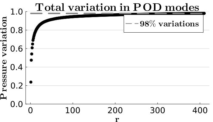
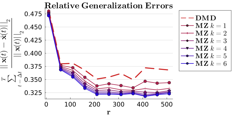
Figure 3: Variance contained in the POD modes of the pressure field, and generalization errors varying number of POD observables $r$ and number of memory terms $k$.

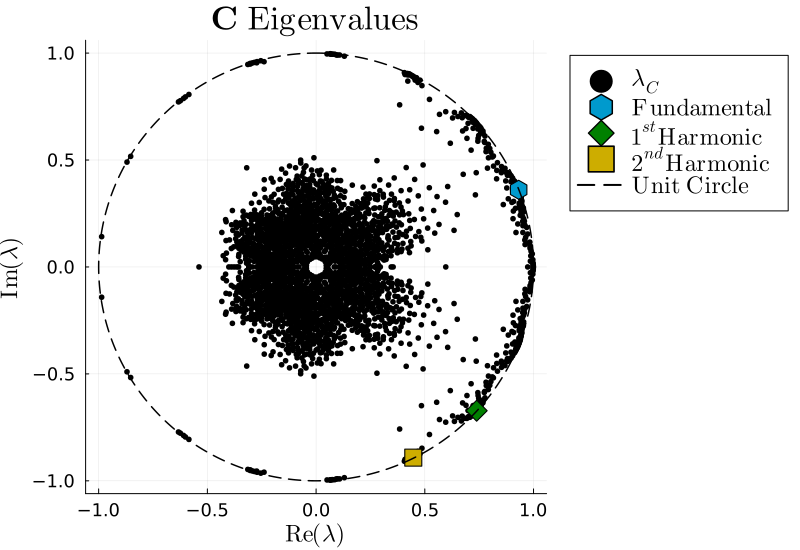
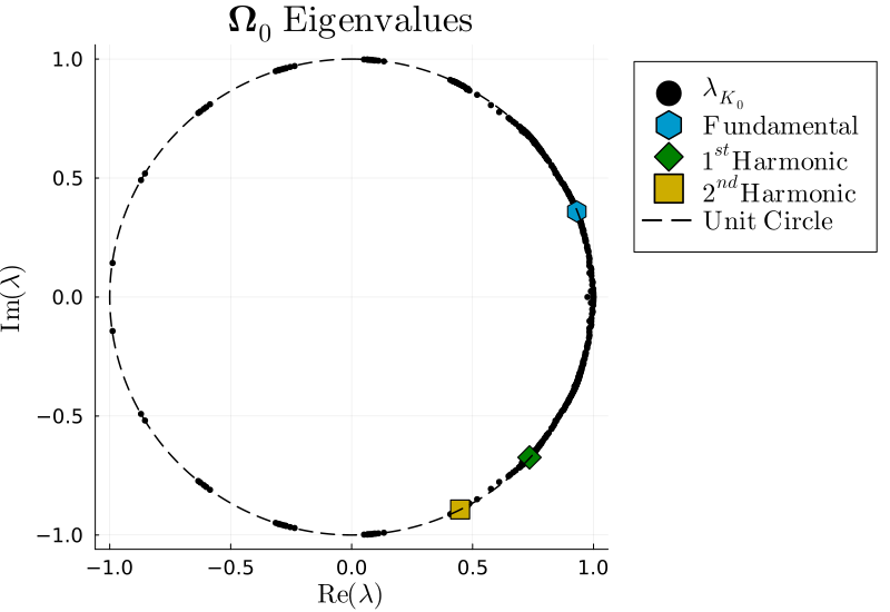
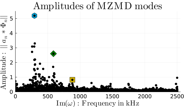
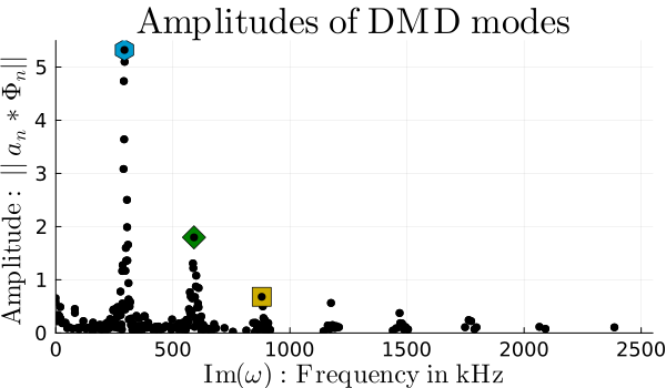
Figure 4: Eigenvalues and amplitudes of MZMD and DMD modes respectively, where the "dominant" modes are uniquely labeled.

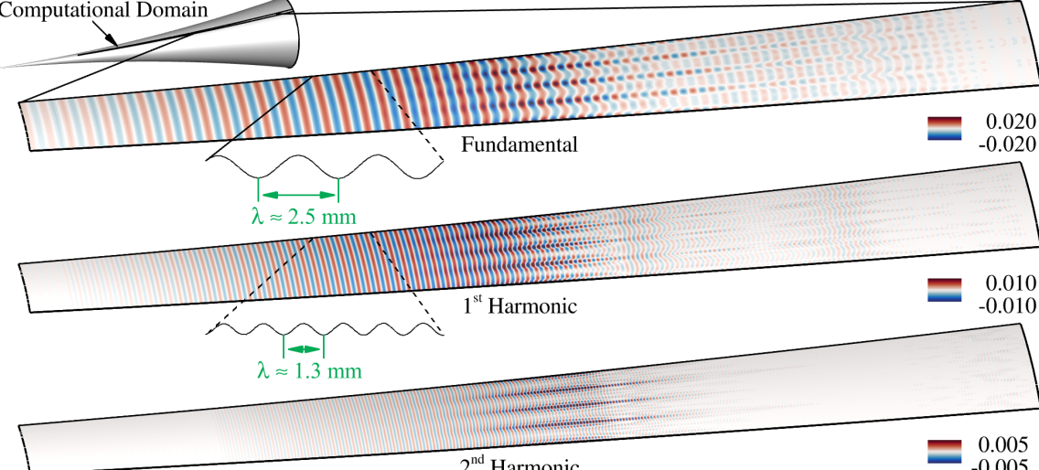
Figure 5: MZMD modes (normalized w.r.t amplitudes) associated with the fundamental frequency (300 kHz), the first (600 kHz), and second (900 kHz) higher harmonics.

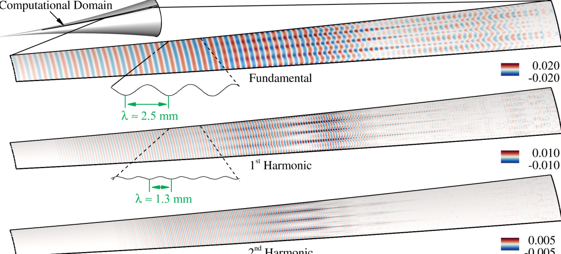
Figure 6: DMD modes (normalized w.r.t amplitudes) associated with the fundamental frequency (300 kHz), the first (600 kHz), and second (900 kHz) higher harmonics.

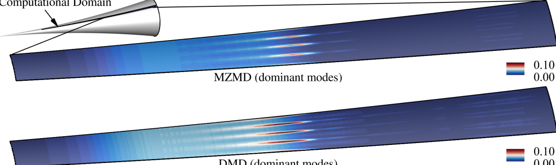
Figure 7: Relative point-wise MSE over time between test set reconstruction using the first three dominant MZMD (top) and DMD (bottom) modes.

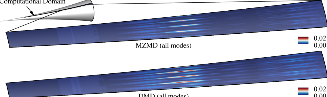
Figure 8: Relative point-wise MSE over time between test set reconstruction using full operators MZMD (top) and DMD (bottom).

6 Conclusion

In this manuscript, we have developed a new modal decomposition technique, MZMD, using the Mori-Zwanzig formalism to extract large scale spatio-temporal structures. We have shown the connection to DMD, and provided an efficient and rigorous procedure for extracting modes of the associated companion matrix of the GLE evolving the states. We have demonstrated that by using MZ memory, MZMD improves the accuracy of predictions over DMD in regions dominated by nonlinear mechanisms of a transitional hypersonic boundary layer. Most importantly, this improved accuracy is achieved using the same number of "dominant" modes, and for nearly the same computational cost. Additionally, MZMD captures memory effects without the computationally expensive use of time delay embeddings. Many future research directions can be explored by adding MZ memory. The relationship established in this work makes it straightforward to implement MZ memory kernels into existing DMD codes. Furthermore, adding physical structure within the MZ operators is also possible using regression as a projection operator (Lin et al., 2022), to enforce physical constraints (Woodward et al., 2023a; Tian et al., 2023).

Acknowledgments. This work has been authored by employees of Triad National Security, LLC which operates Los Alamos National Laboratory (LANL) under Contract No. 89233218CNA000001 with the U.S. Department of Energy/National Nuclear Security Administration. We acknowledge support from LANL’s Laboratory Directed Research and development (LDRD) program, project number 20220104DR, and computational resources from LANL’s Institutional Computing (IC) program.

Declaration of interests. The authors report no conflict of interest.

Appendix A Algorithms

The MZMD algorithm is summerized below.

Algorithm 1 Discrete MZ Algorithm: SVD based observables

1:Select the number of memory terms $k$ (e.g $k=6$)

2:Given snapshots of data: $\bm{X}_{full}=[\bm{x}_{0},...,\bm{x}_{m+k}]$

3:$\bm{X}_{full}\approx\bm{U}_{r}\bm{\Sigma}_{r}\bm{V}_{r}^{*}$ Truncated SVD

4:Using SVD compressed observables (as linear autoencoder): i.e $\bm{G}=\bm{U}_{r}^{*}\bm{X}_{full}$

5:Collect snapshots over $k$ time delays: $\bm{G}_{0}=[\bm{g}_{0},\bm{g}_{1},...,\bm{g}_{m}]$, $\bm{G}_{1}=[\bm{g}_{1},\bm{g}_{2},...,\bm{g}_{m+1}]$, … $\bm{G}_{k}=[\bm{g}_{k},\bm{g}_{k+1},...,\bm{g}_{m+k}]$

6:——————————————————————————————–

7: $\bm{C}_{0}=\bm{G}_{0}\cdot\bm{G}_{0}^{T}$

8:for $i\leftarrow 1,...,k$ do

9:     $\bm{C}_{i}=\bm{G}_{i}\cdot\bm{G}_{0}^{T}$

10:end for

11:$\bm{\Omega}_{0}=\bm{C}_{1}\cdot\bm{C}_{0}^{-1}$

12:for $i\leftarrow 1,...,k$ do

13:     $\bm{\Omega}_{i}=\left[\bm{C}_{i+1}-\sum_{l=0}^{i-1}\bm{\Omega}_{l}\cdot\bm{C}_{i-l}\right]\cdot\bm{C}_{0}^{-1}$

14:end for

15:- Form companion matrix $\bm{C}_{g}$, then compute eigendecomposition $\bm{C}_{g}\bm{W}=\bm{W}\bm{\Lambda}$

16:- MZMD modes: $\bm{\phi}_{i}^{0}=\bm{U}_{r}\bm{w}^{0}_{i}$, where $\bm{w}^{0}_{i}=\bm{P}_{0}\bm{w}_{i}$ and $\bm{P}_{0}=[\bm{I}\hskip 5.69054pt\bm{0}\hskip 5.69054pt...\hskip 5.69054pt\bm{0}]$.

17:- $\bm{g}_{n+1}=\sum_{l=0}^{k}\bm{\Omega}_{l}\bm{g}_{n-l}$ Future prediction in reduced space

18:- $\bm{x}_{n+1}\approx\bm{U}_{r}\bm{g}_{n+1}$ Future state prediction in full state space (all modes).

19:- $\bm{x}_{n+1}\approx\sum_{i}a_{i}\lambda_{i}^{n+1}\bm{\phi}_{i}^{0}$ (selected modes prediction)

References

- Arbabi & Mezić (2017) Arbabi, H. & Mezić, I. 2017 Ergodic theory, dynamic mode decomposition, and computation of spectral properties of the koopman operator. SIAM Journal on Applied Dynamical Systems 16 (4), 2096–2126.
- Bai et al. (2000) Bai, Z., Sleijpen, G., van der Vorst, H., Lippert, R. & Edelman, A. 2000 9. Nonlinear Eigenvalue Problems, pp. 281–314, arXiv: https://epubs.siam.org/doi/pdf/10.1137/1.9780898719581.ch9.
- Chynoweth et al. (2019) Chynoweth, B.C., Schneider, S.P., Hader, C., Fasel, H.F., Batista, A., Kuehl, J., Juliano, T.J. & Wheaton, B.M. 2019 History and progress of boundary-layer transition on a mach-6 flared cone. Journal of Spacecraft and Rockets 56 (2), 333–346.
- Gloerfelt (2008) Gloerfelt, Xavier 2008 Compressible proper orthogonal decomposition/Galerkin reduced-order model of self-sustained oscillations in a cavity. Physics of Fluids 20 (11), 115105.
- Hader & Fasel (2018) Hader, C. & Fasel, H. 2018 Towards simulating natural transition in hypersonic boundary layers via random inflow disturbances. JFM 847.
- Hader & Fasel (2019) Hader, Christoph & Fasel, Hermann F. 2019 Direct numerical simulations of hypersonic boundary-layer transition for a flared cone: fundamental breakdown. Journal of Fluid Mechanics 869, 341–384.
- Holmes & Lumley (2012) Holmes, P. & Lumley, J. 2012 Turbulence Coherent Structures, Dynamical Systems and Symmetry. Cambridge.
- Kalashnikova et al. (2014) Kalashnikova, Irina, Arunajatesan, Srinivasan, Barone, Matthew Franklin, van Bloemen Waanders, Bart Gustaaf & Fike, Jeffrey A. 2014 Reduced order modeling for prediction and control of large-scale systems. .
- Kamb et al. (2020) Kamb, M., Kaiser, E., Brunton, S. L. & Kutz, J. N. 2020 Time-delay observables for koopman: Theory and applications. SIAM Journal on Applied Dynamical Systems 19 (2), 886–917.
- Kimmel & Kendall (1991) Kimmel, R. & Kendall, J. 1991 Nonlinear disturbances in a hypersonic boundary layer. AIAA 1991-0320.
- Le Clainche & Vega (2017) Le Clainche, S. & Vega, J. M. 2017 Higher order dynamic mode decomposition. SIAM J. Appl. Dyn. Syst. 16 (2), 882–925.
- Li et al. (2019) Li, Xiaocan, Wang, Shuo & Cai, Yinghao 2019 Tutorial: Complexity analysis of singular value decomposition and its variants, arXiv: 1906.12085.
- Lin et al. (2021) Lin, Y.T., Tian, Y., Livescu, D. & Anghel, M. 2021 Data-driven learning for the mori–zwanzig formalism: A generalization of the koopman learning framework. SIAM J. Appl. Dyn. Syst. 20 (4), 2558–2601.
- Lin et al. (2022) Lin, Yen Ting, Tian, Yifeng & Livescu, Daniel 2022 Regression-based projection for learning mori–zwanzig operators.
- Mori (1965) Mori, Hazime 1965 Transport, collective motion, and brownian motion. Progress of theoretical physics 33 (3), 423–455.
- Morkovin et al. (1994) Morkovin, M.V., Reshotko, E. & Herbert, T. 1994 Transition in open flow systems-a reassessment. Bull. Am. Phys. Soc. 39, 1882.
- Parish & Duraisamy (2017) Parish, Eric J. & Duraisamy, Karthik 2017 Non-markovian closure models for large eddy simulations using the mori-zwanzig formalism. Phys. Rev. Fluids 2, 014604.
- Rowley et al. (2009) Rowley, C. W., Mezić, I., Bagheri, S., Schlatter, P. & Henningson, D.S. 2009 Spectral analysis of nonlinear flows. JFM 641, 115–127.
- Schmid (2010) Schmid, PETER J. 2010 Dynamic mode decomposition of numerical and experimental data. Journal of Fluid Mechanics 656, 5–28.
- Subbareddy et al. (2014) Subbareddy, P.K., Bartkowicz, M.D. & Candler, G.V. 2014 Direct numerical simulation of high-speed transition due to an isolated roughness element. JFM 748, 848–878.
- Taira et al. (2017) Taira, K., Brunton, S. L., Dawson, S. T.M., Rowley, C. W., Colonius, T., McKeon, B. J., Schmidt, O. T., Gordeyev, S., Theofilis, V. & Ukeiley, L. S. 2017 Modal analysis of fluid flows: An overview. AIAA Journal 55 (12), 4013–4041.
- Tian et al. (2021a) Tian, Yifeng, Lin, Yen Ting, Anghel, Marian & Livescu, Daniel 2021a Data-driven learning of mori-zwanzig operators for isotropic turbulence. Physics of Fluids 33 (12), 125118.
- Tian et al. (2021b) Tian, Yifeng, Livescu, Daniel & Chertkov, Michael 2021b Physics-informed machine learning of the lagrangian dynamics of velocity gradient tensor. Phys. Rev. Fluids 6, 094607.
- Tian et al. (2023) Tian, Yifeng, Woodward, Michael, Stepanov, Mikhail, Fryer, Chris, Hyett, Criston, Livescu, Daniel & Chertkov, Michael 2023 Lagrangian large eddy simulations via physics-informed machine learning. Proceedings of the National Academy of Sciences 120 (34), e2213638120.
- Towne et al. (2018) Towne, A., Schmidt, O. T. & Colonius, T. 2018 Spectral proper orthogonal decomposition and its relationship to dynamic mode decomposition and resolvent analysis. JFM 847, 821–867.
- Williams et al. (2015) Williams, M.O, Kevrekidis, I.G. & Rowley, C.W. 2015 A Data–Driven Approximation of the Koopman Operator: Extending Dynamic Mode Decomposition. J. Nonlinear Sci. 25 (6), 1307–1346.
- Woodward et al. (2023a) Woodward, M., Tian, Y., Hyett, C., Fryer, C., Stepanov, M., Livescu, D. & Chertkov, M. 2023a Physics-informed machine learning with smoothed particle hydrodynamics: Hierarchy of reduced lagrangian models of turbulence. Phys. Rev. Fluids 8, 054602.
- Woodward et al. (2023b) Woodward, M., Tian, Y., Mohan, A.T., Lin, Y.T., Hader, C., Livescu, D., Fasel, H.F. & Chertkov, M. 2023b Data-Driven Mori-Zwanzig: Approaching a Reduced Order Model for Hypersonic Boundary Layer Transition.
- Woodward et al. (2023c) Woodward, M., Tian, Y., Ting, Lin, Y.T., Mohan, A.T., Hader, C., Fasel, H., Chertkov, M. & Livescu, D. 2023c Data-Driven Mori-Zwanzig: Reduced Order Modeling of Sparse Sensors Measurements for Boundary Layer Transition. AIAA 2023-4256.
- Wu et al. (2021) Wu, Z., Brunton, S. L. & Revzen, S. 2021 Challenges in dynamic mode decomposition. Journal of The Royal Society Interface 18 (185), 20210686.
- Yu et al. (2019) Yu, Ming, Huang, Wei-Xi & Xu, Chun-Xiao 2019 Data-driven construction of a reduced-order model for supersonic boundary layer transition. Journal of Fluid Mechanics 874, 1096–1114.
- Zwanzig (1973) Zwanzig, R. 1973 Nonlinear generalized langevin equations. J. Stat. Phys. 9 (3), 215–220.