A number of discrepancies have emerged between lattice computations and data-driven dispersive evaluations of the RBC/UKQCD intermediate-window-hadronic contribution to the muon anomalous magnetic moment. It is therefore interesting to obtain data-driven estimates for the light-quark-connected and strange-plus-disconnected components of this window quantity, allowing for a more detailed comparison between the lattice and data-driven approaches. The aim of this paper is to provide these estimates, extending the analysis to several other window quantities, including two windows designed to focus on the region in which the two-pion contribution is dominant. Clear discrepancies are observed for all light-quark-connected contributions considered, while good agreement with lattice results is found for strange-plus-disconnected contributions to the quantities for which corresponding lattice results exist. The largest of these discrepancies is that for the RBC/UKQCD intermediate window, where, as previously reported, our data-driven result, $a_{\mu}^{W1,{\rm lqc}}=198.9(1.1)\times 10^{-10}$, is in significant tension with the results of 8 different recent lattice determinations. Our strategy is the same as recently employed in obtaining data-driven estimates for the light-quark-connected and strange-plus-disconnected components of the full leading-order hadronic vacuum polarization contribution to the muon anomalous magnetic moment. Updated versions of those earlier results are also presented, for completeness.

I Introduction

There have been many developments since the publication of the first of the Fermilab E989 measurements of the muon anomalous magnetic moment [2, 3] and the publication of the White-Paper (WP) Standard-Model (SM) estimate [4] that preceded it. A lattice computation of the leading-order hadronic vacuum polarization (HVP) contribution $a_{\mu}^{\rm HVP}$ by the BMW collaboration resulted in a value that would bring the total SM expectation much closer to the experimental value [5], if one assumes that the $5\sigma$ discrepancy between the world average of the experimental value and the WP value is due to the leading-order HVP contribution. In addition, there now exist a large number of lattice computations [5, 7, 8, 9, 10, 11, 12, 13, 14] of the RBC/UKQCD intermediate window quantity [15] that are in relatively good agreement with each other, but not in agreement with data-driven estimates [16].

The lattice computation of $a_{\mu}^{\rm HVP}$ is carried out by breaking down the total contribution into several building blocks. The primary building blocks are the isospin-symmetric light- and strange-quark connected and three-flavor disconnected parts, together with smaller charm and bottom contributions (both of which also have connected and disconnected components). Electromagnetic (EM) and strong-isospin-breaking (SIB) effects (collectively, isospin-breaking (IB) effects) are taken into account perturbatively, with corrections linear in the fine-structure constant $\alpha$ and the up-down quark mass difference $m_{u}-m_{d}$ sufficiently precise for the current desired level of accuracy. In contrast, the data-driven dispersive approach is based on an analysis of hadronic electro-production data on a channel-by-channel basis ($\pi^{+}\pi^{-}$, $\pi^{+}\pi^{-}\pi^{0}$, etc.) up to squared hadronic invariant masses, $s$, just below $4$ GeV² and inclusive data above that point. To gain a better understanding of the emerging discrepancies, it is useful to find out in more detail which of the lattice components are most strongly in tension with data-driven estimates. For this, it is necessary to reorganize the data-driven approach such as to provide direct estimates for the building blocks that constitute the lattice-based computation of $a_{\mu}^{\rm HVP}$. It is, in addition, of interest to consider auxillary lattice quantities that focus on the region in which the two-pion contribution dominates, in order to further sharpen our understanding of the source(s) of the lattice-dispersive discrepancy.

In recent work, we have obtained such data-driven estimates for the isospin-symmetric light-quark connected (“lqc” for short) [17] and strange connected plus (three-flavor-) disconnected contributions [18] to $a_{\mu}^{\rm HVP}$. We refer to the latter as the strange plus disconnected contribution in what follows, or “s+lqd” for short. While the strange plus disconnected contribution was found to be in good agreement with most lattice computations (with comparable errors), the light-quark connected contribution differed significantly from the lattice result of Ref. [5]. This state of affairs provides a strong motivation for obtaining similar light-quark connected and strange plus disconnected data-driven estimates for various window quantities such as the RBC/UKQCD intermediate window, where, as mentioned above, a growing number of lattice collaborations finds values not in agreement with data-driven estimates.

The aim of this paper is to provide data-driven values for a number of light-quark connected and strange plus disconnected window quantities, specifically, the original RBC/UKQCD intermediate window quantity, the longer-distance window quantity proposed in Ref. [10], and two window quantities introduced in Ref. [19], and compare these with corresponding lattice values where available. The result for the data-based light-quark connected contribution to the intermediate window obtained with our method has already been reported in a recent letter [20]. Here we extend the results to other windows, to the strange plus disconnected contributions and provide several additional details.

The analysis of Refs. [17, 18] was based on the tabulated exclusive-mode hadronic contributions to $a_{\mu}^{\rm HVP}$ made available in Refs. [21] (DHMZ) and [22] (KNT). Such a tabulation is not publicly available for any of the window quantities considered in this paper. One therefore needs access to the exclusive-mode spectral distributions for all hadronic channels contributing to the HVP in order to evaluate the channel-by-channel contributions to these window quantities, which then, following the strategy of Refs. [17, 18], can be used to obtain the light-quark connected and strange plus disconnected contributions to these window quantities. In this paper, we will use the exclusive-mode spectral distributions and covariances from the 2019 KNT analysis (KNT19 in what follows). As analogous exclusive-mode information from DHMZ is not available to us, we are unable to present estimates based on DHMZ data. In this respect the analysis presented here differs from that in Refs. [17, 18], in which both KNT19- and DHMZ-based values for the light-quark connected and strange plus disconnected contributions to $a_{\mu}^{\rm HVP}$ were obtained.

Of course, both the KNT and DHMZ data contain EM and SIB effects. These have to be estimated and subtracted in order to arrive at purely hadronic and isospin-symmetric estimates for the various window quantities. Both types of corrections have been recently considered in Refs. [23, 24, 25, 26]. The existence of as-yet-unquantified exclusive-mode contributions (see, e.g., the discussions in Refs. [24, 25] and the appendix of Ref. [17]) means insufficient experimental information is currently available to extract inclusive EM corrections, and we thus choose to rely on available lattice estimates for the EM corrections we employ; these will be the only lattice data we will make use of in this paper. As we will see, these corrections are very small. Additional IB corrections, in which a combination of EM and SIB effects occur, are amenable to data-driven treatment. Useful information on the sum of EM and SIB contributions in the two-pion channel, which is expected to be dominated by its SIB component, is provided by Ref. [23]. We will use these results in assessing and subtracting this sum. Other such EM+SIB corrections will also be discussed below. We will use a definition of QCD in the isospin limit in which the pion mass is equal to the physical $\pi^{0}$ mass. To first order in IB, i.e., to ${\cal O}(\alpha)$ and ${\cal O}(m_{u}-m_{d})$, this is sufficient to define an unambiguous split between EM and SIB corrections.

This paper is organized as follows. In Sec. II we define the window quantities of interest in this paper (Sec. II.1), and remind the reader how to relate the lqc and s+lqd parts of the EM spectral function to its isospin components. In Sec. III we present our results, based on the KNT19 data, for the exclusive-channel contributions to the lqc and s+lqd parts of our window quantities in the region below $s=(1.937)^{2}$ GeV², treating first the modes for which the isospin can be identified through $G$-parity (Sec. III.1), and then the isospin-ambiguous modes (Sec. III.2). Above $s=(1.937)^{2}$ GeV² we employ perturbation theory, which is discussed in Sec. III.3. IB corrections are discussed in detail in Sec. IV. We then compare our results with recent lattice results for the same quantities in Sec. VI, and conclude in Sec. VII. There are two appendices, one tabulating intermediate results in addition to those explained in the main text, and one with a more detailed discussion of the $\pi^{0}\gamma$ and $\eta\gamma$ exclusive modes.

II Review

We define the window quantities we will consider in this paper in Sec. II.1, and recall how to write the light-quark connected and strange plus disconnected spectral functions in terms of the $I=1$ and $I=0$ components.

II.1 Windows

The leading-order HVP contribution $a_{\mu}^{\rm HVP}$ to $a_{\mu}$ can be written, in dispersive form, as [27, 28, 29]

$$a_{\mu}^{\rm HVP}=\frac{4\alpha^{2}m_{\mu}^{2}}{3}\int_{m_{\pi}^{2}}^{\infty}ds\,\frac{\hat{K}(s)}{s^{2}}\rho_{\rm EM}(s)\ ,$$ (1)

where $m_{\pi}$ is the neutral pion mass. Here $\rho_{\rm EM}(s)$ is the inclusive EM-current hadronic spectral function

$$\rho_{\rm EM}(s) = \frac{1}{12\pi^{2}}R(s)\ ,$$ (2)

$$R(s) = \frac{3s}{4\pi\alpha^{2}}\,\sigma^{(0)}[e^{+}e^{-}\rightarrow\mbox{hadrons}(+\gamma)]\ ,$$

where $R(s)$ is the $R$ ratio obtained from the bare inclusive hadronic electroproduction cross section $\sigma^{(0)}[e^{+}e^{-}\rightarrow\mbox{hadrons}(+\gamma)]$, and $\hat{K}(s)$ is a known smoothly varying kernel with $\hat{K}(4m_{\pi}^{2})\approx 0.63$ at the two-pion threshold and $\lim_{s\to\infty}\hat{K}(s)=1$. Equivalently, $a_{\mu}^{\rm HVP}$ can be expressed in terms of the Euclidean-time two-point correlation function [30]

$$C(t)=\frac{1}{3}\sum_{i=1}^{3}\int d^{3}x\langle j_{i}^{\rm EM}(\vec{x},t)j_{i}^{\rm EM}(0)\rangle=\frac{1}{2}\int_{m_{\pi}^{2}}^{\infty}ds\,\sqrt{s}\,e^{-\sqrt{s}t}\,\rho_{\rm EM}(s)\quad(t>0)\ ,$$ (3)

of the EM current, $j_{i}^{\rm EM}(\vec{x},t)$, as

$$a_{\mu}^{\rm HVP}=2\int_{0}^{\infty}dt\,w(t)C(t)\ ,$$ (4)

where $w(t)$ is a known function related to $\hat{K}(s)$ by

$$\frac{\hat{K}(s)}{s^{2}}=\frac{3\sqrt{s}}{4\alpha^{2}m_{\mu}^{2}}\int_{0}^{\infty}dt\,w(t)\,e^{-\sqrt{s}t}\ .$$ (5)

We note that $C(t)$ has a $\delta$-function singularity at $t=0$, but this does not contribute to Eq. (4) since $w(t)\sim t^{4}$ for $t\to 0$.

Our first class of window quantities is defined by inserting the window function [15]

$$W(t;t_{0},t_{1};\Delta)=\frac{1}{2}\left(\tanh\frac{t-t_{0}}{\Delta}-\tanh\frac{t-t_{1}}{\Delta}\right)$$ (6)

with $t_{1}>t_{0}>0$ into Eq. (4):

$$a_{\mu}^{W}(t_{0},t_{1};\Delta) = 2\int_{0}^{\infty}dt\,W(t;t_{0},t_{1};\Delta)\,w(t)C(t)$$

$$= \int_{m_{\pi}^{2}}^{\infty}ds\,\rho_{\rm EM}(s)\,\sqrt{s}\int_{0}^{\infty}dt\,W(t;t_{0},t_{1};\Delta)\,w(t)\,e^{-\sqrt{s}t}$$

$$= \frac{4\alpha^{2}m_{\mu}^{2}}{3}\int_{m_{\pi}^{2}}^{\infty}ds\,\frac{\hat{K}(s)}{s^{2}}\,\widetilde{W}(s;t_{0},t_{1};\Delta)\,\rho_{\rm EM}(s)\ ,$$

where

$$\widetilde{W}(s;t_{0},t_{1};\Delta)=\frac{\int_{0}^{\infty}dt\,W(t;t_{0},t_{1};\Delta)\,w(t)\,e^{-\sqrt{s}t}}{\int_{0}^{\infty}dt\,w(t)\,e^{-\sqrt{s}t}}$$ (8)

is the window function in $s$-space.

In what follows, we will consider two window quantities of this type, $a_{\mu}^{W1}$ and $a_{\mu}^{W2}$, corresponding to the window functions $W1$ and $W2$ obtained using the choices

$$W1:\qquad t_{0}=0.4~{}\mbox{fm}\ ,\quad t_{1}=1.0~{}\mbox{fm}\ ,\quad\Delta=0.15~{}\mbox{fm}\ ,$$ (9a)

$$W2:\qquad t_{0}=1.5~{}\mbox{fm}\ ,\quad t_{1}=1.9~{}\mbox{fm}\ ,\quad\Delta=0.15~{}\mbox{fm}\ ,$$ (9b)

for the external parameters, $t_{0}$, $t_{1}$ and $\Delta$, in Eq. (6). The first of these, $a_{\mu}^{W1}$, is the RBC/UKQCD intermediate window quantity introduced in Ref. [15]. The second, $a_{\mu}^{W2}$, is the alternate longer distance “intermediate” window quantity introduced in Ref. [10] designed to be better suited to treatment using chiral perturbation theory.

We will also consider window quantities $I_{\widehat{W}}$,

$$I_{\widehat{W}}=\int_{m_{\pi}^{2}}^{\infty}ds\,\widehat{W}(s)\,\rho_{\rm EM}(s)\ ,$$ (10)

involving weights, $\widehat{W}(s)$, defined directly as functions of $s$ and having the form

$$\widehat{W}(s;\{t_{i}\},\{x_{i}\})=\frac{1}{2}\sum_{i=1}^{n}x_{i}\sqrt{s}e^{-t_{i}\sqrt{s}}\ ,$$ (11)

with $\{t_{i}\}$ a set of positive numbers. Using Eq. (3) it follows that

$$I_{\widehat{W}}=\sum_{i=1}^{n}x_{i}C(t_{i})\ ,$$ (12)

thus providing a sum rule that allows for a comparison between the spectral integral $I_{\widehat{W}}$ and the weighted sum of $n$ values of the correlation function $C(t)$ that can be computed on the lattice [19]. By choosing $n$ and the sets $\{t_{i}\}$ and $\{x_{i}\}$ judiciously, weights can be constructed to focus on particular regions of interest in $s$. A key advantage of the form Eq. (11) is that it turns out to be possible to obtain such localization in $s$ using sets $\{t_{i}\}$ which entirely avoid the large-$t$ region in which lattice $C(t)$ errors deteriorate [19], thus simultaneously controlling errors on the lattice side of the sum rule Eq. (12). The lattice errors corresponding to four such choices, $W^{\prime}_{15}$, $W^{\prime}_{25}$, $\widehat{W}_{15}$ and $\widehat{W}_{25}$, all focusing on the region around the $\rho$ peak, were investigated in Ref. [19], using available light-quark connected $C(t)$ results, with $\widehat{W}_{15}$ and $\widehat{W}_{25}$ found to produce the smallest relative lattice errors. We thus focus on these cases in what follows. Both involve an $n=5$-fold sum, and the choice

$$\{t_{i}\}=\{3,\ 6,\ 9,\ 12,\ 15\}\ \mbox{GeV}^{-1}$$ (13)

for the set $\{t_{i}\}$. The weight $\widehat{W}_{15}$ is then obtained by choosing

$$\{x_{i}^{(15)}\}=\{-78.8487,\ 5688.30,\ 2223.96,\ -36638.0,\ 8047.38\}\ ,$$ (14)

and $\widehat{W}_{25}$ by choosing

$$\{x_{i}^{(25)}\}=\{44.8916,\ 590.933,\ -3373.53,\ 3716.86,\ 8047.38,\ 879.149\}\ .$$ (15)

With the inclusive spectral function $\rho_{\rm EM}(s)$ one can obtain data-driven values for $a_{\mu}^{W1}$, $a_{\mu}^{W2}$, $I_{\widehat{W}_{15}}$ and $I_{\widehat{W}_{25}}$. For $a_{\mu}^{W1}$ (and a number of other weights which we will not consider here) this was done in Ref. [16]. Here we are interested in obtaining, for each of the weights we consider, the light-quark connected and strange plus disconnected building blocks.

II.2 Light-quark connected and strange plus disconnected spectral functions

First, we review the ingredients of the basic idea from Refs. [17, 18]. The decomposition of the three-flavor EM current into its isospin $I=1$ and $I=0$ parts, produces related decompositions of $C(t)$ and $\rho_{\rm EM}(s)$, into pure $I=1$, pure $I=0$ and mixed-isospin parts

$$C(t) = C^{I=1}(t)+C^{\rm MI}(t)+C^{I=0}(t)\ ,$$ (16)

$$\rho_{\rm EM}(s) = \rho_{\rm EM}^{I=1}(s)+\rho_{\rm EM}^{\rm MI}(s)+\rho_{\rm EM}^{I=0}(s)\ ,$$

where in an isospin symmetric world the mixed-isospin (MI) components vanish. Weighted integrals over $\rho_{\rm EM}$, of course, inherit this same decomposition.

In the isospin limit, the $I=0$ contribution to the light-quark connected (lqc) part of $C(t)$ is exactly $1/9$ times the corresponding $I=1$ contribution. The strange (connected plus disconnected) plus light-quark disconnected (s+lqd) contribution is, similarly, the difference of the $I=0$ contribution and $1/9$ times the $I=1$ contribution. The lqc and s+lqd window quantities considered in this paper, which are of the form (II.1) with $W=W1$ or $W=W2$, or of the form (10) with $\widehat{W}=\widehat{W}_{15}$ or $\widehat{W}=\widehat{W}_{25}$, are thus given, in the isospin limit, by the expressions

$$a_{\mu}^{W,\rm lqc} = \frac{4\alpha^{2}m_{\mu}^{2}}{3}\int_{m_{\pi}^{2}}^{\infty}ds\,\frac{\hat{K}(s)}{s^{2}}\,\widetilde{W}(s;t_{0},t_{1};\Delta)\,\rho_{\rm EM}^{\rm lqc}(s)\ ,$$ (17)

$$a_{\mu}^{W,\rm s+lqd} = \frac{4\alpha^{2}m_{\mu}^{2}}{3}\int_{m_{\pi}^{2}}^{\infty}ds\,\frac{\hat{K}(s)}{s^{2}}\,\widetilde{W}(s;t_{0},t_{1};\Delta)\,\rho_{\rm EM}^{\rm s+lqd}(s)\ ,$$

and

$${\cal{I}}_{\widehat{W}}^{\rm lqc} = \int_{m_{\pi}^{2}}^{\infty}ds\,\widehat{W}(s)\,\rho^{\rm lqc}_{\rm EM}(s)\ ,$$ (18)

$${\cal{I}}_{\widehat{W}}^{\rm s+lqd} = \int_{m_{\pi}^{2}}^{\infty}ds\,\widehat{W}(s)\,\rho^{\rm s+lqd}_{\rm EM}(s)\ ,$$

where

$$\rho^{\rm lqc}_{\rm EM}(s)=\frac{10}{9}\rho_{\rm EM}^{I=1}(s)$$ (19)

and

$$\rho^{\rm s+lqd}_{\rm EM}(s)=\rho_{\rm EM}^{I=0}(s)-\frac{1}{9}\rho_{\rm EM}^{I=1}(s)=\rho_{\rm EM}(s)-\frac{10}{9}\rho_{\rm EM}^{I=1}(s)\ .$$ (20)

The evaluation of the lqc and s+lqd parts of the four window quantities defined in Sec. II.1 thus requires an identification of the separate $I=1$ and $I=0$ components of $\rho_{\rm EM}(s)$. The separation of contributions from all hadronic exclusive modes can, assuming isospin symmetry, be accomplished, up to $\sqrt{s}=1.937$ GeV, using KNT19 exclusive-mode data, as described in the following section. We will then, in Sec. IV, discuss the EM and SIB corrections to our values for the lqc and s+lqd parts of our window quantities.

III Implementation

In this section, we obtain the lqc and s+lqd parts for all four window quantities, postponing until Sec. IV a consideration of EM and SIB corrections. In Sec. III.1 we collect exclusive-mode contributions from modes which are $G$-parity eigenstates and hence have an unambiguous $I=0$ or $1$ assignment. The separation of contributions from modes which are not $G$-parity eigenstates into separate $I=0$ and $I=1$ components is detailed in Sec. III.2.

III.1 Modes with unambiguous isospin

As in Ref. [18], we take advantage of the fact that exclusive modes with positive (negative) $G$-parity have $I=1$ ($I=0$). The contributions of such modes to the $I=1$ and $I=0$ parts of $a_{\mu}^{W1}$ are shown in Table 1. Analogous tables are provided for the other window quantities in App. A. From these results, we obtain the following $G$-parity unambiguous contributions to our window quantities:

$$\left[a_{\mu}^{W1,\rm lqc}\right]_{G\rm{\mathchar 45\relax par}} = \frac{10}{9}\times 168.24(72)\times 10^{-10}=186.94(80)\times 10^{-10}\ ,$$

$$\left[a_{\mu}^{W2,\rm lqc}\right]_{G\rm{\mathchar 45\relax par}} = \frac{10}{9}\times 85.05(33)\times 10^{-10}=94.50(36)\times 10^{-10}\ ,$$

$$\left[I_{\widehat{W}_{15}}^{\rm lqc}\right]_{G\rm{\mathchar 45\relax par}} = \frac{10}{9}\times 39.37(14)\times 10^{-2}=43.75(15)\times 10^{-2}\ ,$$

$$\left[I_{\widehat{W}_{25}}^{\rm lqc}\right]_{G\rm{\mathchar 45\relax par}} = \frac{10}{9}\times 67.29(30)\times 10^{-3}=74.76(34)\times 10^{-3}\ ,$$ (21)

and

$$\left[a_{\mu}^{W1,\rm s+lqd}\right]_{G\rm{\mathchar 45\relax par}} = \left[20.69(37)-\frac{168.24(72)}{9}\right]\times 10^{-10}=1.99(38)\times 10^{-10}\ ,$$

$$\left[a_{\mu}^{W2,\rm s+lqd}\right]_{G\rm{\mathchar 45\relax par}} = \left[6.23(14)-\frac{85.05(33)}{9}\right]\times 10^{-10}=-3.22(14)\times 10^{-10}\ ,$$

$$\left[I_{\widehat{W}_{15}}^{\rm s+lqd}\right]_{G\rm{\mathchar 45\relax par}} = \left[3.77(08)-\frac{39.37(14)}{9}\right]\times 10^{-2}=-0.609(84)\times 10^{-2}\ ,$$

$$\left[I_{\widehat{W}_{25}}^{\rm s+lqd}\right]_{G\rm{\mathchar 45\relax par}} = \left[8.92(16)-\frac{67.29(30)}{9}\right]\times 10^{-3}=1.45(16)\times 10^{-3}\ ,$$ (22)

$I=1$ modes $X$	$[a_{\mu}^{W1}]_{X}\times 10^{10}$	$I=0$ modes $X$	$[a_{\mu}^{W1}]_{X}\times 10^{10}$
low-$s$ $\pi^{+}\pi^{-}$	0.02(00)	low-$s$ $3\pi$	0.00(00)
$\pi^{+}\pi^{-}$	144.13(49)	$3\pi$	18.69(35)
$2\pi^{+}2\pi^{-}$	9.29(13)	$2\pi^{+}2\pi^{-}\pi^{0}$ (no $\omega$, $\eta$)	0.61(06)
$\pi^{+}\pi^{-}2\pi^{0}$	11.94(48)	$\pi^{+}\pi^{-}3\pi^{0}$ (no $\eta$)	0.39(07)
$3\pi^{+}3\pi^{-}$ (no $\omega$)	0.14(01)	$3\pi^{+}3\pi^{-}\pi^{0}$ (no $\omega$, $\eta$)	0.00(00)
$2\pi^{+}2\pi^{-}2\pi^{0}$ (no $\eta$)	0.83(11)	$\eta\pi^{+}\pi^{-}\pi^{0}$ (no $\omega$)	0.44(05)
$\pi^{+}\pi^{-}4\pi^{0}$ (no $\eta$)	0.13(13)	$\eta\omega$	0.19(01)
$\eta\pi^{+}\pi^{-}$	0.85(03)	$\omega(\rightarrow npp)2\pi$	0.08(01)
$\eta 2\pi^{+}2\pi^{-}$	0.05(01)	$\omega 2\pi^{+}2\pi^{-}$	0.00(00)
$\eta\pi^{+}\pi^{-}2\pi^{0}$	0.07(01)	$\eta\phi$	0.25(01)
$\omega(\rightarrow\pi^{0}\gamma)\pi^{0}$	0.53(01)	$\phi\rightarrow unaccounted$	0.02(02)
$\omega(\rightarrow npp)3\pi$	0.10(02)
$\omega\eta\pi^{0}$	0.15(03)
TOTAL:	168.24(72)	TOTAL:	20.69(37)

Table 1: $G$-parity-unambiguous exclusive-mode contributions to $a_{\mu}^{W1}$ for $\sqrt{s}\leq 1.937$ GeV using KNT19 exclusive-mode data. Entries in units of $10^{-10}$. The notation “npp” is KNT shorthand for “non-purely-pionic.”

III.2 Modes with ambiguous isospin

We now consider those exclusive modes which are not $G$-parity eigenstates, and thus have no definite isospin. Associated contributions to the various window quantities thus, in general, have both $I=1$ and $I=0$ components, which must be separated to complete determinations of the corresponding lqc and s+lqd contributions. Modes of this type in the KNT19 exclusive-mode region are $\pi^{0}\gamma$, $\eta\gamma$, $N\bar{N}$ and those containing a $K\bar{K}$ pair.

For the numerically most important modes of the latter type, $K\bar{K}$ and $K\bar{K}\pi$, the $I=0/I=1$ separation is facilitated by use of additional experimental input ($\tau^{-}\rightarrow K^{-}K^{0}\nu_{\tau}$ data [33] for $K\bar{K}$ and BaBar Dalitz plot analysis results [34] for $K\bar{K}\pi$), following the strategy of Ref. [18], outlined briefly below.

For the modes $P\gamma$ with $P=\pi^{0},\,\eta$, the cross sections in the KNT19 exclusive-mode region of relevance to the weighted integrals considered in this paper are strongly dominated by contributions involving intermediate $V=\rho$, $\omega$ and $\phi$ meson exchange. Vector-meson-dominance (VMD) representations of the $e^{+}e^{-}\rightarrow P\gamma$ cross sections, which require as input only $m_{P}$, the vector meson masses and widths and known experimental $V\rightarrow e^{+}e^{-}$ and $V\rightarrow P\gamma$ decay widths, turn out to saturate the corresponding KNT19 exclusive-mode integrals considered here, confirming the reliability of the VMD representation. The $I=0$, $I=1$ and MI contributions to those integrals can thus be determined from the parts of the VMD representations involving the squared modulus of the sum of $\omega$ and $\phi$ contributions to the amplitude, the squared modulus of the $\rho$ contribution to the amplitude, and the interference terms between those contributions, respectively. The VMD representation of the cross sections, together with the numerical values of the required external inputs, are detailed in Appendix B. As we will see below, the $I=0$ contribution dominates these integrals for all four window quantities considered in this paper.

For the (much smaller) contributions from other (“residual”) $G$-parity-ambiguous exclusive-modes, $X$, where additional external experimental input is not available, we follow Ref. [18] in employing a “maximally conservative” assessment of the $I=1$/$I=0$ separation, based on the observation that the $I=1$ part of the mode $X$ contribution to $\rho_{\rm EM}(s)$ necessarily lies between $0$ and the full contribution. The mode $X$ lqc and s$+$lqd contributions to $\rho_{\rm EM}(s)$ then necessarily lie in the ranges:

$$\left[\rho^{\rm lqc}_{\rm EM}\right]_{X} = \left(\frac{5}{9}\pm\frac{5}{9}\right)\left[\rho_{\rm EM}\right]_{X}\ ,$$ (23)

$$\left[\rho^{\rm s+lqd}_{\rm EM}\right]_{X} = \left(\frac{4}{9}\pm\frac{5}{9}\right)\left[\rho_{\rm EM}\right]_{X}\ .$$

These bounds produce related “maximally conservative” bounds for weighted exclusive-mode lqc and s+lqd integrals involving weights, $W$, having fixed sign in the region of nonzero $\left[\rho_{\rm EM}(s)\right]_{X}$:

$$\left[a_{\mu}^{W,\rm lqc}\right]_{X} = \left(\frac{5}{9}\pm\frac{5}{9}\right)\left[a_{\mu}^{W}\right]_{X}\ ,$$ (24)

$$\left[a_{\mu}^{W,\rm s+lqd}\right]_{X} = \left(\frac{4}{9}\pm\frac{5}{9}\right)\left[a_{\mu}^{W}\right]_{X}\ .$$

The maximally conservative $I=1$/$I=0$ separation bounds, while generally valid, would, if applied to all $G$-parity-ambiguous modes, produce errors so large that our estimates for the lqc and s+lqd parts of the window quantities would be uninteresting. Fortunately, for those modes where this would be an issue, more experimental information is available, allowing us to dramatically reduce the uncertainty on the $I=1$/$I=0$ separation.

Let us first consider the $K\bar{K}$ modes, $K^{+}K^{-}$ and $K^{0}\bar{K}^{0}$. Independent information on the $K\bar{K}$ contribution to the $I=1$ spectral function is available from data on the differential distribution for the decay $\tau\to K^{-}K^{0}\nu_{\tau}$ measured by BaBar [33]. Using the CVC (conserved vector current) relation, these results can be converted into the $I=1$ $e^{+}e^{-}\to K\bar{K}$ contribution to $R(s)$. Using the results of Ref. [33] up to $s=2.7556$ GeV², and a KNT19-based maximally conservative assessment of $I=1$ contributions for $s$ from $2.7556$ GeV² to $s=(1.937)^{2}$ GeV², we find, following the steps of Sec. IV.B of Ref. [18], the results

$$\left[a_{\mu}^{W1,\rm lqc}\right]_{K\bar{K}} = \frac{10}{9}\left(0.465(29)+0.055(55)\right)\times 10^{-10}=0.578(69)\times 10^{-10}\ ,$$ (25)

$$\left[a_{\mu}^{W2,\rm lqc}\right]_{K\bar{K}} = \frac{10}{9}\left(0.0241(17)+0.00035(35)\right)\times 10^{-10}=0.0271(20)\times 10^{-10}\ ,$$

$$\left[I_{\widehat{W}_{15}}^{\rm lqc}\right]_{K\bar{K}} = \frac{10}{9}\left(0.0158(12)-0.0023(23)\right)\times 10^{-2}=0.0150(29)\times 10^{-2}\ ,$$

$$\left[I_{\widehat{W}_{25}}^{\rm lqc}\right]_{K\bar{K}} = \frac{10}{9}\left(0.209(13)+0.024(24)\right)\times 10^{-3}=0.259(30)\times 10^{-3}\ ,$$

where in each case the first number in parentheses is the contribution from the BaBar $\tau$ data in the region $s\leq 2.7556$ GeV², and the second number is the result of the maximally conservative assessment of the contribution from $s=2.7556$ GeV² to $(1.937)^{2}$ GeV², obtained using KNT19 data.

For the s+lqd parts, using the second equation of Eq. (20), we find

$$\left[a_{\mu}^{W1,\rm s+lqd}\right]_{K\bar{K}} = \left(19.13(15)-0.578(69)\right)\times 10^{-10}=18.55(17)\times 10^{-10}\ ,$$ (26)

$$\left[a_{\mu}^{W2,\rm s+lqd}\right]_{K\bar{K}} = \left(2.612(21)-0.0271(20)\right)\times 10^{-10}=2.585(21)\times 10^{-10}\ ,$$

$$\left[I_{\widehat{W}_{15}}^{\rm s+lqd}\right]_{K\bar{K}} = \left(2.213(18)-0.015(29)\right)\times 10^{-2}=2.198(18)\times 10^{-2}\ ,$$

$$\left[I_{\widehat{W}_{25}}^{\rm s+lqd}\right]_{K\bar{K}} = \left(8.642(70)-0.259(30)\right)\times 10^{-3}=8.383(76)\times 10^{-3}\ ,$$

where the first number in parentheses in each case is the full $K^{+}K^{-}$ plus $K^{0}\bar{K}^{0}$ contribution from the KNT19 data, and the second number is that of Eq. (25). By comparing Eq. (25), which is pure $I=1$, and Eq. (26), which is dominated by $I=0$, we see that clearly the $K\bar{K}$ channels are dominated by $I=0$. This is expected because of the $I=0$ $\phi$ resonance.

Our next case to consider is that of the $K\bar{K}\pi$ modes. The separation of the corresponding cross sections into their $I=0$ and $I=1$ parts was carried out by BaBar in Ref. [34], and, as in Ref. [18], we obtain the $I=1$ (and hence the lqc) contributions, up to $s=(1.937)^{2}\ {\rm GeV}^{2}$,

$$\left[a_{\mu}^{W1,\rm lqc}\right]_{K\bar{K}\pi} = \frac{10}{9}\left[a_{\mu}^{W1,I=1}\right]_{K\bar{K}\pi}=0.521(86)\times 10^{-10}\ ,$$ (27)

$$\left[a_{\mu}^{W2,\rm lqc}\right]_{K\bar{K}\pi} = \frac{10}{9}\left[a_{\mu}^{W2,I=1}\right]_{K\bar{K}\pi}=0.0060(10)\times 10^{-10}\ ,$$

$$\left[I_{\widehat{W}_{15}}^{\rm lqc}\right]_{K\bar{K}\pi} = \frac{10}{9}\left[I_{\widehat{W}_{15}}^{I=1}\right]_{K\bar{K}\pi}=-0.0152(25)\times 10^{-2}\ ,$$

$$\left[I_{\widehat{W}_{25}}^{\rm lqc}\right]_{K\bar{K}\pi} = \frac{10}{9}\left[I_{\widehat{W}_{25}}^{I=1}\right]_{K\bar{K}\pi}=0.229(38)\times 10^{-3}\ .$$

For the s+lqd $K\bar{K}\pi$ contributions from the same region, we find

$$\left[a_{\mu}^{W1,\rm s+lqd}\right]_{K\bar{K}\pi} = \left(1.714(74)-0.521(86)\right)\times 10^{-10}=1.19(11)\times 10^{-10}\ ,$$ (28)

$$\left[a_{\mu}^{W2,\rm s+lqd}\right]_{K\bar{K}\pi} = \left(0.01846(82)-0.0060(10)\right)\times 10^{-10}=0.0124(13)\times 10^{-10}\ ,$$

$$\left[I_{\widehat{W}_{15}}^{\rm s+lqd}\right]_{K\bar{K}\pi} = \left(-0.0536(24)+0.0152(25)\right)\times 10^{-2}=-0.0384(35)\times 10^{-2}\ ,$$

$$\left[I_{\widehat{W}_{25}}^{\rm s+lqd}\right]_{K\bar{K}\pi} = \left(0.753(33)-0.229(38)\right)\times 10^{-3}=0.524(50)\times 10^{-3}\ ,$$

where the first number in parentheses in each case is the full $K\bar{K}\pi$ contribution obtained using KNT19 data, and the second number is that of Eq. (27).

A small improvement, relative to the maximally conservative assessment (24), can also be obtained for contributions from the $K\bar{K}2\pi$ modes by making use of the measured $e^{+}e^{-}\to\phi\pi\pi$ mode cross sections [35], which allow the purely $I=0$ contribution resulting from $e^{+}e^{-}\to\phi[\rightarrow K\bar{K}]\pi\pi$ to be subtracted from the KNT19 $K\bar{K}2\pi$ total and the maximally conservative separation into $I=1$ and $I=0$ components applied only to the remainder. Following Ref. [18], we find

$$\left[a_{\mu}^{W1,\rm lqc}\right]_{K\bar{K}2\pi} = 0.60(60)\times 10^{-10}\ ,$$ (29)

$$\left[a_{\mu}^{W2,\rm lqc}\right]_{K\bar{K}2\pi} = 0.0031(31)\times 10^{-10}\ ,$$

$$\left[I_{\widehat{W}_{15}}^{\rm lqc}\right]_{K\bar{K}2\pi} = -0.028(28)\times 10^{-2}\ ,$$

$$\left[I_{\widehat{W}_{25}}^{\rm lqc}\right]_{K\bar{K}2\pi} = 0.26(26)\times 10^{-3}\ ,$$

and

$$\left[a_{\mu}^{W1,\rm s+lqd}\right]_{K\bar{K}2\pi} = 0.58(60)\times 10^{-10}\ ,$$ (30)

$$\left[a_{\mu}^{W2,\rm s+lqd}\right]_{K\bar{K}2\pi} = 0.0032(31)\times 10^{-10}\ ,$$

$$\left[I_{\widehat{W}_{15}}^{\rm s+lqd}\right]_{K\bar{K}2\pi} = -0.027(28)\times 10^{-2}\ ,$$

$$\left[I_{\widehat{W}_{25}}^{\rm s+lqd}\right]_{K\bar{K}2\pi} = 0.25(26)\times 10^{-3}\ .$$

The final G-parity-ambiguous modes for which additional external experimental input provides an improved isospin decomposition are the two radiative modes $\pi^{0}\gamma$ and $\eta\gamma$. Using the accurate VMD representations of the $e^{+}e^{-}\rightarrow\pi^{0}\gamma$ and $e^{+}e^{-}\rightarrow\eta\gamma$ cross sections detailed in Appendix B, and employing 2023 PDG input [36], we find the following results for the lqc and s+lqd contributions from these modes:

$$\left[a_{\mu}^{W1,\rm lqc}\right]_{\pi^{0}\gamma+\eta\gamma} = \left(0.074(13)+0.063(0)\right)\times 10^{-10}=0.137(13)\times 10^{-10}\ ,$$ (31)

$$\left[a_{\mu}^{W2,\rm lqc}\right]_{\pi^{0}\gamma+\eta\gamma} = \left(0.029(5)+0.021(0)\right)\times 10^{-10}=0.050(5)\times 10^{-10}\ ,$$

$$\left[I_{\widehat{W}_{15}}^{\rm lqc}\right]_{\pi^{0}\gamma+\eta\gamma} = \left(0.018(3)+0.013(0)\right)\times 10^{-2}=0.031(3)\times 10^{-2}\ ,$$

$$\left[I_{\widehat{W}_{25}}^{\rm lqc}\right]_{\pi^{0}\gamma+\eta\gamma} = \left(0.031(6)+0.028(0)\right)\times 10^{-3}=0.059(6)\times 10^{-3}\ ,$$

and

$$\left[a_{\mu}^{W1,\rm s+lqd}\right]_{\pi^{0}\gamma+\eta\gamma} = \left(1.25(6)+0.25(1)\right)\times 10^{-10}\,=\,1.50(6)\times 10^{-10}\ ,$$ (32)

$$\left[a_{\mu}^{W2,\rm s+lqd}\right]_{\pi^{0}\gamma+\eta\gamma} = \left(0.54(3)+0.04(0)\right)\times 10^{-10}\,=\,0.58(3)\times 10^{-10}\ ,$$

$$\left[I_{\widehat{W}_{15}}^{\rm s+lqd}\right]_{\pi^{0}\gamma+\eta\gamma} = \left(0.32(2)+0.03(0)\right)\times 10^{-2}\,=\,0.35(2)\times 10^{-2}\ ,$$

$$\left[I_{\widehat{W}_{25}}^{\rm s+lqd}\right]_{\pi^{0}\gamma+\eta\gamma} = \left(0.53(3)+0.11(0)\right)\times 10^{-3}\,=\,0.64(3)\times 10^{-3}\ ,$$

where the first term in each intermediate expression is the $\pi^{0}\gamma$ contribution and the second term the $\eta\gamma$ one.

Contributions from the remaining $G$-parity-ambiguous modes, $K\bar{K}3\pi$, $\omega(\rightarrow npp)K\bar{K}$, $\eta(\rightarrow npp)K\bar{K}$ (no $\phi$), $p\bar{p}$, $n\bar{n}$, and low-$s$ $\pi^{0}\gamma$ and $\eta\gamma$, which are very small, are listed for completeness in Appendix A.

The sums of all exclusive-mode contributions below $s=(1.937)^{2}$ GeV² for the lqc window quantities are obtained from Eqs. (III.1), (25), (27), (29),  (31) and the further exclusive-mode contributions listed in Appendix A. The results are

$$\left[a_{\mu}^{W1,\rm lqc}\right]_{\rm excl} = 188.82(1.01)\times 10^{-10}\ ,$$ (33)

$$\left[a_{\mu}^{W2,\rm lqc}\right]_{\rm excl} = 94.60(36)\times 10^{-10}\ ,$$

$$\left[I_{\widehat{W}_{15}}^{\rm lqc}\right]_{\rm excl} = 43.75(16)\times 10^{-2}\ ,$$

$$\left[I_{\widehat{W}_{25}}^{\rm lqc}\right]_{\rm excl} = 75.59(43)\times 10^{-3}\ .$$

For the s+lqd window quantities, similarly, we obtain from Eqs. (III.1),  (26), (28), (30),  (32) and the further exclusive-mode contributions listed in Appendix A, the results

$$\left[a_{\mu}^{W1,\rm s+lqd}\right]_{\rm excl} = 23.85(74)\times 10^{-10}\ ,$$ (34)

$$\left[a_{\mu}^{W2,\rm s+lqd}\right]_{\rm excl} = -0.04(14)\ ,$$

$$\left[I_{\widehat{W}_{15}}^{\rm s+lqd}\right]_{\rm excl} = 1.875(92)\times 10^{-2}\ ,$$

$$\left[I_{\widehat{W}_{25}}^{\rm s+lqd}\right]_{\rm excl} = 11.26(32)\times 10^{-3}\ .$$

III.3 Perturbative contribution above $s=(1.937)^{2}$ GeV²

Above $s=(1.937)^{2}$ GeV² we use perturbation theory to evaluate (three-flavor) contributions to the window quantities. We employ massless perturbation theory, using the five-loop result of Ref. [37] for the Adler function, following the steps outlined in Refs. [17, 18]. Above $s=(1.937)^{2}$ GeV² and up to the charm-quark threshold, perturbation theory agrees well with inclusive BES [38, 39] and KEDR [40] $R(s)$ measurements, although the agreement with recent, more precise, BESIII results [41] is less good. We find for these perturbative contributions, using $\alpha_{s}(m_{\tau}^{2})=0.3139(71)$ [36]

$$\left[a_{\mu}^{W1,\rm lqc}\right]_{\rm pert.th.} = 10.896\times 10^{-10}\ ,$$ (35)

$$\left[a_{\mu}^{W2,\rm lqc}\right]_{\rm pert.th.} = 0.00757\times 10^{-10}\ ,$$

$$\left[I_{\widehat{W}_{15}}^{\rm lqc}\right]_{\rm pert.th.} = -0.574\times 10^{-2}\ ,$$

$$\left[I_{\widehat{W}_{25}}^{\rm lqc}\right]_{\rm pert.th.} = 3.658\times 10^{-3}\ .$$

Error estimates along the lines of Ref. [18] lead to errors of the order of 0.1% of the central values in Eq. (35), which are small enough that they can be ignored in our final results. In order to obtain the s+lqd perturbative contributions, the values in Eq. (35) have to be multiplied by $(2/9)(9/10)=1/5$ [17]. For completeness, we provide the resulting values:

$$\left[a_{\mu}^{W1,\rm s+lqd}\right]_{\rm pert.th.} = 2.179\times 10^{-10}\ ,$$ (36)

$$\left[a_{\mu}^{W2,\rm s+lqd}\right]_{\rm pert.th.} = 0.00151\times 10^{-10}\ ,$$

$$\left[I_{\widehat{W}_{15}}^{\rm s+lqd}\right]_{\rm pert.th.} = -0.115\times 10^{-2}\ ,$$

$$\left[I_{\widehat{W}_{25}}^{\rm s+lqd}\right]_{\rm pert.th.} = 0.732\times 10^{-3}\ .$$

Although the use of perturbation theory above $s=(1.937)^{2}$ GeV² is supported by the good agreement with the inclusive $R(s)$ data of Refs. [38, 39, 40], the slight tension with the recent BESIII data [41] hints at possible residual duality violations (DVs) even in the inclusive region. While our estimates for residual DV contributions to $a_{\mu}^{\rm HVP,lqc}$ and $a_{\mu}^{\rm HVP,s+lqd}$ showed these to be small, DVs represent an intrinsic limitation of perturbation theory. We will thus include the central values of our DV estimates in our final results, assigning them an uncertainty of 100%. The assigned DV uncertainty totally dominates our estimate of the uncertainty associated with the use of perturbation theory in the inclusive region.

For lqc contributions, which involve only the $\rho_{\rm EM}^{I=1}(s)$ spectral function, we obtain our DV estimates using the results of finite-energy sum-rule fits performed in Ref. [42] using an improved version of the $I=1$ charged-current spectral function, $\rho_{ud;V}(s)$, obtained mainly from $\tau$ decay data, and related by CVC to $\rho_{\rm EM}^{I=1}(s)$ by $\rho_{\rm EM}^{I=1}(s)=\frac{1}{2}\rho_{ud;V}(s)$. Following the procedure described in Sec. IIIA of Ref. [17], we find for our estimates of the DV contributions to $a_{\mu}^{W,{\rm lqc}}$ and $I_{W}^{\rm lqc}$ the results

$$\left[a_{\mu}^{W1,\rm lqc}\right]_{\rm DVs} = 0.162(77)\times 10^{-10}\ ,$$ (37)

$$\left[a_{\mu}^{W2,\rm lqc}\right]_{\rm DVs} = 0.00034(20)\times 10^{-10}\ ,$$

$$\left[I_{\widehat{W}_{15}}^{\rm lqc}\right]_{\rm DVs} = -0.0092(44)\times 10^{-2}\ ,$$

$$\left[I_{\widehat{W}_{25}}^{\rm lqc}\right]_{\rm DVs} = 0.069(33)\times 10^{-3}\ .$$

Possible residual DV corrections to the use of perturbation theory in the inclusive region will be present in both the $I=1$ and $I=0$ contributions to $a_{\mu}^{W,{\rm s+lqd}}$ and $I_{W}^{\rm s+lqd}$. To estimate the combination of these effects, we will use the results of the finite-energy sum-rule fits to KNT $\rho_{\rm EM}(s)$ data performed in Ref. [43]. We find

$$\left[a_{\mu}^{W1,\rm s+lqd}\right]_{\rm DVs} = -0.17(5)\times 10^{-10}\ ,$$ (38)

$$\left[a_{\mu}^{W2,\rm s+lqd}\right]_{\rm DVs} = -0.0004(1)\times 10^{-10}\ ,$$

$$\left[I_{\widehat{W}_{15}}^{\rm s+lqd}\right]_{\rm DVs} = 0.010(3)\times 10^{-2}\ ,$$

$$\left[I_{\widehat{W}_{25}}^{\rm s+lqd}\right]_{\rm DVs} = -0.07(2)\times 10^{-3}\ .$$

The results of Eqs. (35) and (36), supplemented by the central values from Eqs. (37) and Eqs. (38), which serve as our estimates for the DV-induced perturbative uncertainties, have to be added to those of Eqs. (33) and (34), respectively. As noted above, we take the total error on the perturbative plus DV contributions to be equal to the (absolute value of the) central values of the DV contributions, which are always larger than the DV errors quoted above. This produces the following total lqc and s+lqd contributions, not yet corrected for EM and SIB effects:

$$a_{\mu}^{W1,\rm lqc} = 199.88(1.02)\times 10^{-10}\ ,$$ (39)

$$a_{\mu}^{W2,\rm lqc} = 94.61(36)\times 10^{-10}\ ,$$

$$I_{\widehat{W}_{15}}^{\rm lqc} = 43.17(16)\times 10^{-2}\ ,$$

$$I_{\widehat{W}_{25}}^{\rm lqc} = 79.32(43)\times 10^{-3}\ ,$$

and

$$a_{\mu}^{W1,\rm s+lqd} = 25.86(76)\times 10^{-10}\ ,$$ (40)

$$a_{\mu}^{W2,\rm s+lqd} = -0.04(14)\times 10^{-10}\ ,$$

$$I_{\widehat{W}_{15}}^{\rm s+lqd} = 1.770(92)\times 10^{-2}\ ,$$

$$I_{\widehat{W}_{25}}^{\rm s+lqd} = 11.92(32)\times 10^{-3}\ .$$

IV Electromagnetic and strong isospin-breaking effects

The results of Eqs. (39) and  (40) were obtained using experimental data and thus contain EM and SIB effects. These effects need to be estimated and subtracted to obtain lqc and s+lqd results that can be compared directly to those obtained from isospin-symmetric lattice QCD without QED. We employ the same strategy to carry out these subtractions as that used in Refs. [17, 18], which is predicated on the observation that, to first order in IB, SIB contributions occur only in the MI component of $\rho_{\rm EM}(s)$, while EM contributions are present in all of the pure $I=1$, pure $I=0$ and MI components. IB corrections to the window quantities we consider are thus of two types. Those present in the pure $I=1$ and pure $I=0$ contributions are, to first order in IB, purely EM, and require only an estimate of the inclusive combination of EM contributions from all exclusive modes, with no need for a further breakdown of these corrections into those associated with individual exclusive modes. The MI corrections, in contrast, require removing from the nominal pure $I=1$ and pure $I=0$ sums obtained above exclusive-mode IB contributions which, in fact, represent MI contaminations of those sums. Examples of such MI contaminations are the two-pion and three-pion contributions resulting from the $\rho-\omega$-mixing-induced processes $e^{+}e^{-}\rightarrow\omega\rightarrow\rho\rightarrow 2\pi$ and $e^{+}e^{-}\rightarrow\rho\rightarrow\omega\rightarrow 3\pi$. MI corrections to the lqc and s+lqd combinations thus require identifying the combined EM+SIB IB parts of the individual exclusive-mode contributions relevant to each, and cannot be carried out using inclusive versions of the EM or SIB contributions, or their sum. We do, however, expect the MI contaminations to be dominated by contributions from the two- and three-pion modes, where the narrowness of the $\omega$ peak and the small $\rho-\omega$ mass difference lead to a strong enhancement of IB contributions from the $\rho-\omega$ region. We will estimate MI two- and three-pion corrections from this region using fits to data (which, of course, produce assessments of the EM+SIB sum) and employ a generic $O(1\%)$ estimate for the size of MI contamination in the contributions from other exclusive modes, which (i) lie higher in the spectrum, and hence have contributions suppressed by the falloff in $s$ of the weights considered here, and (ii) are not subject to any narrow-nearby-resonance enhancements. Given the very small size of EM and SIB corrections to the perturbative contribution to the lqc and s+lqd spectral functions, we will ignore IB corrections from the $s\geq(1.937)^{2}\ {\rm GeV}^{2}$ (inclusive) region.

In view of the above discussion, we treat separately the corrections for EM effects in the nominally pure $I=1$ and $I=0$ contributions and those for EM+SIB MI contamination, discussing the former in Sec. IV.1 and the latter in Sec. IV.2. As mentioned above, we follow many lattice groups and define our isospin limit of QCD as one in which all pions have a mass equal to the physical neutral pion mass.

IV.1 $I=1$ and $I=0$ electromagnetic corrections

To quantify and subtract the EM contributions present in the pure $I=1$ and $I=0$ parts of the window quantities of interest, we rely on information from the lattice results obtained in Ref. [5]. While some EM effects have been estimated from experimental data [23, 26, 25], additional potentially significant EM effects have not and we thus consider it unavoidable to rely on lattice EM data for the EM corrections. The existence of significant cancellations amongst the set of data-based EM contribution estimates detailed in Refs. [24, 25] also argues in favor of using the inclusive lattice result since that result necessarily includes contributions from all sources, including those not currently amenable to data-based estimates, and whose relative role might be enhanced by the strong cancellations amongst the currently quantified contributions. This constitutes our only use of lattice data in obtaining our estimates for the lqc and s+lqd window quantities; as we will see, these corrections are very small.

For the RBC/UKQCD intermediate window $W1$, the lqc EM correction has been obtained directly in Ref. [5]. The result is

$$\Delta_{\rm EM}a_{\mu}^{W1,\rm lqc}=0.035(59)\times 10^{-10}\ .$$ (41)

For the s+lqd EM correction for the same window, the relevant lattice data are also given in Ref. [5]. Using exactly the same strategy as in Ref. [18], we find

$$\Delta_{\rm EM}a_{\mu}^{W1,\rm s+lqd}=0.012(11)\times 10^{-10}\ .$$ (42)

As Ref. [5] did not obtain the relevant lattice estimates for EM contributions to the other window quantities considered here, we do not have equivalent estimates for these other quantities. However, if we compare the $W1$ corrections with Eqs. (39) and (40), we see that the central value of the lqc EM correction is $\sim$30 times smaller than the error in Eqs. (39), while the central value of the s+lqd correction is $\sim$60 times smaller than the error in Eqs. (40). Since the relative errors on the other window quantities in Eqs. (39) and (40) are of order the same size as or larger than those in the $W1$ quantities, we will assume that EM corrections to the pure $I=1$ and $I=0$ contributions to these quantities can be safely neglected, and ignore these EM corrections in the rest of this paper. This assumption should be particularly safe for the s+lqd contributions, where the diagrammatic analysis of Ref. [18] shows the existence of generic strong cancellations, for example in the numerically dominant light-quark EM valence-valence connected and disconnected contributions.

IV.2 The mixed-isospin (MI) correction

As in Ref. [18], we expect the MI EM+SIB correction to be dominated by contributions from the 2-pion and 3-pion exclusive modes, where there are potentially strong enhancements due to $\rho-\omega$ interference in the $\rho-\omega$ resonance region, and where contributions from that region are more strongly weighted than are those of other modes, lying at higher $s$, in all the window quantities considered in this paper. Such IB $\rho-\omega$ region $2\pi$ and $3\pi$ contributions can be estimated from the interference terms in fits to the $e^{+}e^{-}\rightarrow 2\pi$ and $e^{+}e^{-}\rightarrow 3\pi$ electroproduction cross sections associated with the $\rho-\omega$-mixing-induced IB processes $e^{+}e^{-}\rightarrow\omega\rightarrow\rho\rightarrow 2\pi$ and $e^{+}e^{-}\rightarrow\rho\rightarrow\omega\rightarrow 3\pi$, which, to first order in $\alpha$ and $m_{u}-m_{d}$, produce contributions lying entirely in the MI contribution, $\rho_{\rm EM}^{\rm MI}$, of Eq. (16).

For the window quantity $a_{\mu}^{W1}$, the $\rho-\omega$-mixing-enhanced, MI two-pion exclusive-mode contribution has been obtained in Refs. [23, 25] from fits to two-pion electroproduction data employing a dispersively constrained representation of the pion form factor incorporating the effect of $\rho-\omega$ mixing. The result,

$$\left[a_{\mu}^{W1}\right]_{\pi\pi}^{\rm MI}=0.86(6)\times 10^{-10}\ ,$$ (43)

represents a MI contamination to be subtracted from the nominal $I=1$ exclusive-mode sum, and hence produces a correction

$$\Delta_{\pi\pi}^{\rm MI}a_{\mu}^{W1,{\rm lqc}}=-{\frac{10}{9}}\times 0.86(6)\times 10^{-10}=-0.96(7)\times 10^{-10}$$ (44)

to the nominal $a_{\mu}^{W1,{\rm lqc}}$ result of Eqs. (39). In spite of its enhancement by $\rho-\omega$ mixing, this correction is only $\sim 0.6\%$ of the total two-pion contribution to $a_{\mu}^{W1}$. We thus consider it extremely safe to assume that the magnitude of the sum of MI corrections to the nominal $I=1$ sum from other exclusive modes having no analogous narrow-nearby-resonance enhancements is less than $1\%$ of the sum, $25.68\times 10^{-10}$, of contributions to $a_{\mu}^{W1}$ from those modes. We thus add a further uncertainty $\pm(10/9)\times 0.26\times 10^{-10}=\pm 0.29\times 10^{-10}$ to that in Eq. (44) and take as our final estimate for the MI correction to the pre-IB-corrected $a_{\mu}^{W1,{\rm lqc}}$ value of Eq. (39), the result

$$\Delta^{\rm MI}a_{\mu}^{W1,{\rm lqc}}=-0.96(7)(29)\times 10^{-10}\ .$$ (45)

This result is compatible within errors with the expectation, $-0.753(43)\times 10^{-10}$, for the SIB part of the MI lqc correction implied by the lattice result of Ref. [5] for the SIB contribution to $a_{\mu}^{W1,{\rm lqc}}$, and hence with the expected dominance of the MI EM+SIB lqc correction by its SIB component. Neglecting the very small pure $I=1$ EM correction of Eq. (41), we obtain the IB-corrected result

$$a_{\mu}^{W1,\rm lqc} = \left(199.88(1.02)-0.96(0.30)\right)\times 10^{-10}=198.9(1.1)\times 10^{-10}\ .$$ (46)

Two-pion MI IB corrections due to $\rho-\omega$ mixing based on the analysis of Ref. [23, 25] have also been made available to us for the other three window quantities [44] considered here. In these cases, there are no lattice results to compare with. The resulting MI contributions to the nominal $I=1$ sums are $0.767(31)\times 10^{-10}$ for the $W2$ window quantity, and $0.331(13)\times 10^{-2}$ and $0.300(20)\times 10^{-3}$ for the $\widehat{W}_{15}$ and $\widehat{W}_{25}$ window quantities. To obtain the corresponding lqc IB corrections, these need to be multiplied by 10/9, and subtracted from the totals in Eq. (39). The non-$2\pi$ exclusive-mode contributions to these quantities are $0.9\times 10^{-10}$, vanishingly small, and $13\times 10^{-3}$ respectively. Taking, as above, 1% of these contributions as a further uncertainty induced by MI IB effects from nominally $I=1$, non-$2\pi$ exclusive modes, leads to our final estimates

$$a_{\mu}^{W2,\rm lqc} = \left(94.61(36)-\frac{10}{9}\times 0.767(32)\right)\times 10^{-10}=93.75(36)\times 10^{-10}\ ,$$

$$I_{\widehat{W}_{15}}^{\rm lqc} = \left(43.17(16)-\frac{10}{9}\times 0.331(13)\right)\times 10^{-2}=42.80(16)\times 10^{-2}\ ,$$

$$I_{\widehat{W}_{25}}^{\rm lqc} = \left(79.32(43)-\frac{10}{9}\times 0.30(13)\right)\times 10^{-3}=78.99(45)\times 10^{-3}\,.$$ (47)

Unlike estimates for the MI corrections for the lqc components of the window quantities considered in this paper, which, as explained above, can be obtained using as key input the results of the dispersively constrained analysis of experimental $2\pi$ electroproduction data detailed in Ref. [23], estimates of the MI corrections for the analogous s+lqd components require also input on what is expected to be the dominant nominally $I=0$ MI correction, namely that from the $3\pi$ exclusive mode. While the fact that $2\pi$ contributions to the window quantities listed in Tables 1, 4, 5 and 6 exceed the corresponding $3\pi$ contributions by factors of $7.0-13.6$, might lead one to expect the $3\pi$ MI corrections to be similarly smaller than the corresponding $2\pi$ MI ones, this is, in fact, unlikely to be the case due to an countervailing numerical enhancement of the relative $\rho-\omega$-mixing-induced $3\pi$ correction.

The existence of this enhancement can be understood as follows. The ratio of the $\rho-\omega$-mixing-induced IB interference contribution to the dominant isospin-conserving (IC) $\rho$ contribution to the $\rho-\omega$-resonance-region $2\pi$ cross sections is proportional to the product $P_{2\pi}\equiv\epsilon_{\rho\omega}f_{\omega}/f_{\rho}$, with $\epsilon_{\rho\omega}$ the parameter characterizing the strength of $\rho-\omega$ mixing and $f_{V}$, $V=\rho,\,\omega$ the vector-meson decay constants, characterizing the strength of the couplings of the $\rho$ and $\omega$ to the EM current. The analogous ratio, of $\rho-\omega$-mixing-induced-IB-interference to $\omega$-dominated IC contributions to the resonance-region 3-pion cross sections, is, in contrast, proportional to the product $P_{3\pi}\equiv\epsilon_{\rho\omega}f_{\rho}/f_{\omega}$. Experimentally (as expected for near-ideal mixing of the vector meson nonet), $f_{\rho}\simeq 3f_{\omega}$. A natural enhancement, by a factor of $P_{3\pi}/P_{2\pi}\simeq 9$, is thus present in the ratio of relative sizes of $\rho-\omega$-mixing-induced resonance-region IB in the $3\pi$ versus $2\pi$ channels. It is thus unlikely that the MI $3\pi$ correction is safely negligible on the scale of the MI $2\pi$ correction.

The $\rho-\omega$-mixing MI corrections in the $3\pi$ channel, relevant for the $I=0$ contribution and thus the s+lqd contribution, have recently been estimated in Refs. [26, 25], for $a_{\mu}^{\rm HVP}$ and $a_{\mu}^{W1}$. For $a_{\mu}^{W1}$, their estimate, which is nominally a contribution to the $I=0$ part of $a_{\mu}^{W1}$, is

$$\left[a_{\mu}^{W1}\right]_{3\pi}^{\rm MI}=-1.03(27)\times 10^{-10}.$$ (48)

From Eqs. (33) and (34) and using Table 1 one finds that the other-than $3\pi$ exclusive-mode contribution for $I=0$ equals $22.53\times 10^{-10}$, 1% of which is $0.23$. We add this as an additional error (in quadrature) to Eq. (48), arriving at $-1.03(35)\times 10^{-10}$. To find the MI correction to the s+lqd part of $a_{\mu}^{W1}$, we need to subtract this, while adding back in $1/10$ times Eq. (45) (cf.   Eq. (20)). This leads to our estimate for the MI correction

$$\Delta^{\rm MI}a_{\mu}^{W1,{\rm s+lqd}}=1.13(36)\times 10^{-10}\ ,$$ (49)

where we combined errors in Eqs. (48) and (45) ignoring correlations. We thus obtain the IB-corrected result

$$a_{\mu}^{W1,\rm s+lqd} = \left(25.86(76)+1.13(36)\right)\times 10^{-10}=27.0(8)\times 10^{-10}\ .$$ (50)

Three-pion MI IB corrections due to $\rho-\omega$ mixing based on the analysis of Refs. [26, 25] have also been made available to us for the other three window quantities [44] considered here. The resulting MI contributions to the nominal $I=0$ sums are $-0.367(101)\times 10^{-10}$ for the $W2$ window quantity, and $-0.230(61)\times 10^{-2}$ and $-0.44(12)\times 10^{-3}$ for the $\widehat{W}_{15}$ and $\widehat{W}_{25}$ window quantities. The non-$3\pi$ exclusive-mode contributions to these quantities are $2.7\times 10^{-10}$, $2.2\times 10^{-2}$ and $10.1\times 10^{-3}$, respectively. Taking, as above, 1% of these contributions as a further uncertainty induced by MI IB effects from nominally $I=0$, non-$3\pi$ exclusive modes, leads to our final estimates

$$a_{\mu}^{W2,\rm s+lqd} = \left(-0.03(14)+0.37(11)+\frac{1}{9}\times 0.767(33)\right)\times 10^{-10}$$

$$= 0.42(18)\times 10^{-10}\ ,$$

$$I_{\widehat{W}_{15}}^{\rm s+lqd} = \left(1.770(92)+0.230(65)+\frac{1}{9}\times 0.331(13)\right)\times 10^{-2}$$

$$= 2.04(11)\times 10^{-2}\ ,$$

$$I_{\widehat{W}_{25}}^{\rm s+lqd} = \left(11.92(32)+0.44(16)+\frac{1}{9}\times 0.30(13)\right)\times 10^{-3}$$

$$= 12.39(36)\times 10^{-3}\,.$$

The terms between parentheses come from Eq. (40), and the results for the MI $I=0$ $3\pi$ and MI $I=1$ $2\pi$ corrections quoted above, respectively.

It is possible to test the treatment of exclusive-mode MI contributions described above by comparing the inclusive MI sums that treatment implies to the corresponding inclusive MI lattice results, available for $a_{\mu}^{\rm HVP}$ and $a_{\mu}^{W1}$ from Ref. [5]. The MI lattice results are obtained by combining the SIB results from Ref. [5] with EM MI estimates obtained using the EM results quoted in Ref. [5], following the diagrammatically based analysis strategy employed in Ref. [18]. The latter analysis yields the result, $-0.49(25)\times 10^{-10}$, obtained already in Ref. [18], for the inclusive MI EM contribution to $a_{\mu}^{\rm HVP}$, and $-0.022(23)\times 10^{-10}$ for the MI EM contribution to $a_{\mu}^{W1}$. For the SIB contributions, which, to first order in IB, are pure MI, we have, summing the quoted connected and disconnected contributions, the lattice results [5]

$$\left[a_{\mu}^{\rm HVP}\right]_{\rm SIB} = 1.93(1.20)\times 10^{-10}\ ,$$ (52)

$$\left[a_{\mu}^{W1}\right]_{\rm SIB} = 0.516(44)\times 10^{-10}\ .$$

The inclusive MI lattice totals are thus

$$\left[a_{\mu}^{\rm HVP}\right]_{\rm MI,latt} = 1.44(1.23)\times 10^{-10}\ ,$$ (53)

$$\left[a_{\mu}^{W1}\right]_{\rm MI,latt} = 0.494(50)\times 10^{-10}\ .$$

In the treatment above, the inclusive MI total is, in contrast, obtained by summing our estimates for the MI $\pi^{0}\gamma$, $\eta\gamma$, $2\pi$ and $3\pi$ exclusive-mode contributions, with an additional uncertainty equal to $1\%$ of the sums of the contributions for all other exclusive modes. The $2\pi$ and $3\pi$ contributions are those detailed above, while the MI $\pi^{0}\gamma$ and $\eta\gamma$ contributions are obtained using the same VMD model used to determine the corresponding $I=0$ and $I=1$ contributions, outlined in Appendix B. The results for the latter are

$$\left[a_{\mu}^{\rm HVP}\right]^{\rm MI}_{\pi^{0}\gamma+\eta\gamma}=\left(0.733(65)+0.067(24)\right)\times 10^{-10}=0.800(69)\times 10^{-10}$$

$$\left[a_{\mu}^{W1}\right]^{\rm MI}_{\pi^{0}\gamma+\eta\gamma}=\left(0.268(24)+0.026(1)\right)\times 10^{-10}=0.294(24)\times 10^{-10}\,,$$ (54)

where the first terms is the $\pi^{0}\gamma$ contribution and the second the $\eta\gamma$ contribution. Combining these results with those from the other modes, we find the following alternate data-driven (dd) results

$$\left[a_{\mu}^{\rm HVP}\right]_{\rm MI,dd} = 1.91(73)(77)\times 10^{-10}\ ,$$ (55)

$$\left[a_{\mu}^{W1}\right]_{\rm MI,dd} = 0.12(28)(49)\times 10^{-10}\ ,$$

where the first error is the quadrature sum of the errors on the MI $\pi^{0}\gamma$, $\eta\gamma$, $2\pi$ and $3\pi$ contributions and the second is our estimate of the uncertainty produced by neglecting MI contributions from all other exclusive modes. The data-driven estimates are compatible within errors with the lattice results in both cases.

V Updates of our previous determinations of $a_{\mu}^{\rm HVP,s+lqd}$, $a_{\mu}^{\rm HVP,lqc}$ and $a_{\mu}^{\rm W1,lqc}$

In Refs. [17, 18, 20] we provided first data-driven estimates for $a_{\mu}^{\rm HVP,lqc}$, $a_{\mu}^{\rm HVP,s+lqd}$ and $a_{\mu}^{\rm W1,lqc}$, respectively. This section updates the results of those analyses, taking into account (i) an improved treatment of the small contributions from the $\pi^{0}\gamma$ and $\eta\gamma$ exclusive modes and (ii) changes in external input for the MI $2\pi$ and $3\pi$ IB corrections. In those earlier analyses, the exclusive-mode $\pi^{0}\gamma$ and $\eta\gamma$ contributions were, based on the dominance of the experimental cross sections by the large $\omega$ and $\phi$ peaks, assigned to the nominally pure $I=0$ category. The VMD representation of those cross sections, outlined in Appendix B, allows for an improved version of this treatment. Because the resulting pure $I=1$ contributions are very small, this improvement has only a small effect on the previous lqc results. It has a larger (though still small) impact on the $a_{\mu}^{\rm HVP,s+lqd}$ result. There have also been two small shifts in the input for the MI $2\pi$ contribution since the preliminary version of the Ref. [23] HVP result used in the $a_{\mu}^{\rm HVP,s+lqd}$ determination of Ref. [18]. The second of these shifts also affects the $a_{\mu}^{\rm HVP,lqc}$ and $a_{\mu}^{\rm W1,lqc}$ results of Refs. [17, 20]. The impacts of these shifts on the lqc results are very small on the scale of the errors on those previous results. Finally, the results of Ref. [26] for the MI $3\pi$ corrections provide a significant improvement to the earlier treatment of those corrections and hence to the reliability of the determination of $a_{\mu}^{\rm HVP,s+lqd}$. The numerical impacts of these changes are quantified below.

Equations (31) and (32) provide the updated versions of the lqc and s+lqd contributions from the $\pi^{0}\gamma$ and $\eta\gamma$ modes. The contributions of these modes to $a_{\mu}^{\rm HVP,lqc}$ and $a_{\mu}^{\rm W1,lqc}$, which were previously taken to be zero, are now $0.36(4)\times 10^{-10}$ and $0.14(1)\times 10^{-10}$, respectively. The updated version of the contribution to $a_{\mu}^{\rm HVP,s+lqd}$ is $4.00(17)\times 10^{-10}$, representing shifts of $-1.16(14)\times 10^{-10}$ and $-1.06(14)\times 10^{-10}$ relative to the old KNT19- and DHMZ-based results of Ref. [18].

The impact of the shift in the MI $2\pi$ contribution to $a_{\mu}^{\rm HVP}$ from the preliminary result, $3.65(67)\times 10^{-10}$, employed in Ref. [18] to the most recent version, $3.79(19)\times 10^{-10}$, quoted in Ref. [25], is a very small upward shift of $0.02\times 10^{-10}$ in the result for $a_{\mu}^{\rm HVP,s+lqd}$ obtained in Ref. [18]. The increase from the initially published result, $3.68(17)\times 10^{-10}$ [23], to the updated $3.79(19)\times 10^{-10}$ version [25], similarly, produces a downward shift of $0.12\times 10^{-10}$ in the result for $a_{\mu}^{\rm HVP,lqc}$ obtained in Ref. [17]. The related increase of the MI $2\pi$ contribution to $a_{\mu}^{W1}$ from the initially published $0.83(6)\times 10^{-10}$ result [23] to the recently updated result, $0.86(6)\times 10^{-10}$ [25], similarly produces a downward shift of $0.03\times 10^{-10}$ in the result for $a_{\mu}^{\rm W1,lqc}$ obtained in Ref. [20].

We turn, finally, to the impact of the improved determination of the MI $3\pi$ contribution of Ref. [26] on the results for $a_{\mu}^{\rm HVP,s+lqd}$ obtained in Ref. [18]. In Ref. [18], the MI $3\pi$ correction was estimated based on a VMD model fit by BaBar to BaBar $e^{+}e^{-}\rightarrow 3\pi$ cross sections [45]. The model employed involved an amplitude consisting of a sum of nominally isospin-conserving (IC) $\omega$, $\phi$ and excited $\omega$ contributions, each proportional to the corresponding propagator, and an IB $\rho$ contribution proportional to the $\rho$ propagator. The MI $3\pi$ correction to $a_{\mu}^{\rm HVP,s+lqd}$ was estimated using results provided by BaBar for the contributions to $a_{\mu}^{\rm HVP}$ obtained using the fitted VMD form with and without the $\rho$ contribution included. The IB $\rho$ contribution in the VMD model used by BaBar, however, does not have the $\rho$-$\omega$ mixing form, and hence presumably represents the $\rho$ part of the partial-fraction decomposition of the underlying IB mixing-induced form. That partial-fraction decomposition would also produce a second IB contribution, proportional to the $\omega$ propagator, the effect of which, in the BaBar model, would be absorbed into the fitted strength of the nominally IC $\omega$ contribution to the amplitude. The squared modulus of the $\omega$ amplitude contribution to BaBar’s fitted VMD representation of the cross sections will thus contain a hidden IB part resulting from the interference of this IB contribution with the corresponding IC part of the $\omega$ contribution to the amplitude. This hidden contribution is missing from the BaBar-fit-based estimate of the MI $3\pi$ contribution to $a_{\mu}^{\rm HVP}$ employed in Ref. [18], but automatically taken into account in the form used in determining that contribution in Refs. [26, 25]. We thus replace the BaBar-fit-based estimate with that obtained in Refs. [26, 25]. This produces a shift of $+2.12(69)\times 10^{-10}$ in the MI $3\pi$ correction to $a_{\mu}^{\rm HVP,s+lqd}$.

Combining the effects of the updates above, we find that $a_{\mu}^{\rm HVP,lqc}$ experiences only a very small $0.2\times 10^{-10}$ upward shift, raising the KNT19- and DHMZ-based results of Ref. [17] from $635.0(2.7)\times 10^{-10}$ to $635.2(2.7)\times 10^{-10}$ and $638.1(4.1)\times 10^{-10}$ to $638.3(4.1)\times 10^{-10}$, respectively. The effect on $a_{\mu}^{W1,\rm lqc}$ is even smaller, shifting the KNT19-based result of Ref. [20], $198.8(1.1)\times 10^{-10}$, to $198.9(1.1)\times 10^{-10}$. The updates have a somewhat larger effect on $a_{\mu}^{\rm HVP,s+lqd}$, with the KNT19- and DHMZ-based results of Ref. [18] shifted upward from $40.1(1.4)(1.3)\times 10^{-10}$ to $41.1(1.4)(0.4)$ and $38.7(1.4)(1.3)_{\rm lin}(0.4)\times 10^{-10}$ to $39.8(1.4)(1.3)_{\rm lin}(0.4)\times 10^{-10}$, respectively. The corresponding results for the isospin-limit disconnected contribution to $a_{\mu}^{\rm HVP}$, obtained by subtracting the lattice average for the strange connected contribution from the s+lqd totals, are, using the same notation for the errors as in Ref. [18], similarly shifted, from $-13.3(1.4)(0.4)\times 10^{-10}$ to $-12.3(1.4)(0.4)\times 10^{-10}$ and $-14.6(1.4)(1.3)_{\rm lin}(0.4)\times 10^{-10}$ to $-13.5(1.4)(1.3)_{\rm lin}(0.4)\times 10^{-10}$.

	$a_{\mu}^{W1,\rm lqc}$	tension
this work	198.9(1.1)
BMW 20	207.3(1.4)	4.7$\sigma$
LM 20	206.0(1.2)	4.4$\sigma$
$\chi$QCD 23	206.7(1.8)	3.7$\sigma$
ABGP 22	206.8(2.2)	3.2$\sigma$
Mainz/CLS 22	207.0(1.5)	4.4$\sigma$
ETMC 22	206.5(1.3)	4.5$\sigma$
FHM 23	206.6(1.0)	5.2$\sigma$
RBC/UKQCD 23	206.36(0.61)	5.9$\sigma$

Table 2: Table of the result of Eq. (46) and lattice results for $a_{\mu}^{W1,\rm lqc}$ from Ref. [5] (BMW 20), Ref. [8] (LM 20), Ref. [9] ($\chi$QCD 23), Ref. [10] (ABGP 22), Ref. [11] (Mainz/CLS 22), Ref. [12] (ETMC 22), Ref. [13] (FHM 23), and Ref. [14] (RBC/UKQCD 23). Units of $10^{-10}$. The third column gives the tension between each of the lattice results and our data-based result, in units of the error on the difference.

VI Comparison with other determinations

For the lqc $W1$ window quantity, $a_{\mu}^{W1,\rm lqc}$, we compare our result, Eq. (46), with recent lattice computations in Table 2 and Fig. 1. We refrain from quoting a lattice average for $a_{\mu}^{W1,\rm lqc}$, but it is clear that there is a discrepancy of about $7\times 10^{-10}$ between the data-based value and lattice results. In the table, we list the tensions between each of the lattice results, and the value of Eq. (46). The tensions are significant and range from $3.2\sigma$ up to $5.9\sigma$.

this work	27.0(8)
RBC/UKQCD 18	26.0(2)
BMW 20	26.32(7)
Mainz/CLS 22	26.87(30)
ETMC 22	26.50(29)

Table 3: Table of the result of Eq. (50) and lattice results for $a_{\mu}^{W1,\rm s+lqd}$ from Ref. [15] (RBC/UKQCD 18), Ref. [5] (BMW 20), Ref. [11] (Mainz/CLS 22), Ref. [12] (ETMC 22). Units of $10^{-10}$.

We also compare the s+lqd quantity $a_{\mu}^{W1,\rm s+lqd}$ of Eq. (50) with results from those collaborations that have computed $a_{\mu}^{W1,\rm s+lqd}$ on the lattice as well, in Table 3 and Fig. 2. The lattice and dispersive results are, in this case, seen to be compatible within errors, as was the case for the related s+lqd quantity, $a_{\mu}^{\rm HVP,s+lqd}$.

Two lattice collaborations have computed $a_{\mu}^{W2,\rm lqc}$, with Ref. [10] finding the value $102.1(2.4)\times 10^{-10}$, and Ref. [13] finding the value $100.7(3.2)\times 10^{-10}$. This is to be compared with the data-based value $93.75(36)\times 10^{-10}$ obtained in Eq. (IV.2), see Fig. 3. Our result displays a tension of $3.4\sigma$ with the result of Ref. [10] and $2.2\sigma$ with the result of Ref. [13].

Finally, up to the pure $I=0$ and $I=1$ EM corrections not included in Eq. (IV.2) but expected to be very small, the lqc results of Eq. (IV.2) for $I_{\widehat{W}_{15}}^{\rm lqc}$ and $I_{\widehat{W}_{25}}^{\rm lqc}$ can be compared to the lattice results obtained from the data of Ref. [10] in Ref. [19]:

$$I_{\widehat{W}_{15}}^{\rm lqc}(\mbox{lattice}) = 46.7(0.7)_{\rm stat\ only}\times 10^{-2}\ ,$$ (56)

$$I_{\widehat{W}_{25}}^{\rm lqc}(\mbox{lattice}) = 82.4(1.0)_{\rm stat\ only}\times 10^{-3}\ ,$$

where the errors are statistical only. These comparison provide further evidence of tension between lattice and data-driven results for lqc contributions, though one should keep in mind that the lattice results were obtained in Ref. [19] without a detailed investigation of systematic errors, which was beyond the scope of that paper.

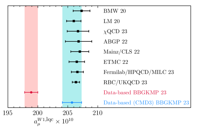
Figure 1: Comparison of the result of Eq. (46) with lattice results for $a_{\mu}^{W1,\rm lqc}$ from Ref. [5] (BMW 20), Ref. [8] (LM 20), Ref. [9] ($\chi$QCD 23), Ref. [10] (ABGP 22), Ref. [11] (Mainz/CLS 22), Ref. [12] (ETMC 22), Ref. [13] (FHM 23), and Ref. [14] (RBC/UKQCD 23). Also shown is the data-based result if the 2-pion data in the interval between 0.33 and 1.2 GeV is replaced by the results from CMD-3 [46].

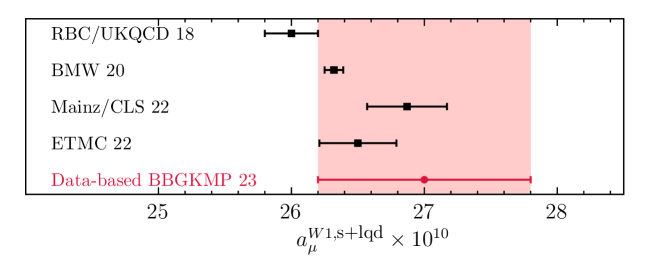
Figure 2: Comparison of the result of Eq. (50) with lattice results for $a_{\mu}^{W1,\rm s+lqd}$ from Ref. [15] (RBC/UKQCD18), Ref. [5] (BMW 20), Ref. [11] (Mainz/CLS 22) and Ref. [12] (ETMC 22).

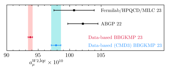
Figure 3: Comparison of the result of Eq. (46) with lattice results for $a_{\mu}^{W2,\rm lqc}$ from Ref. [10] (ABGP 22) and Ref. [13] (FHM 23). Also shown is the data-based result if the 2-pion data in the interval between 0.33 and 1.2 GeV is replaced by the results from CMD-3 [46].

VII Conclusion

In this paper we have obtained data-driven determinations of the lqc and s+lqd contributions to a number of window quantities. Data-driven determinations of such quantities require as input $s$-dependent exclusive-mode distributions, and the results for those determinations reported here are based solely on KNT19 results for those distributions. It would be of interest to repeat the analysis with DHMZ exclusive-mode input, should results for those distributions eventually become publicly available.

Our result for $a_{\mu}^{W1,\rm s+lqd}$ is in good agreement with lattice determinations of this quantity. Similar agreement was found previously for $a_{\mu}^{\rm HVP,s+lqd}$ in Ref. [18]. These are, at present, the only quantities for which lattice s+lqd results exist. It would be of interest to have lattice results, and carry out analogous comparisons, for the other s+lqd quantities considered here.

In contrast to the s+lqd case, our results for the lqc contributions to all four window quantities show tensions with corresponding lattice results. This tension is particularly significant for $a_{\mu}^{W1,{\rm lqc}}$, where, for example, our result differs by $5.9\sigma$ from that of Ref. [14]. Improved lattice determinations of $a_{\mu}^{W2,{\rm lqc}}$, $I_{\widehat{W}_{15}}^{\rm lqc}$ and $I_{\widehat{W}_{25}}^{\rm lqc}$ would be of interest for exploring further the tensions in these cases, especially so for $I_{\widehat{W}_{15}}^{\rm lqc}$ and $I_{\widehat{W}_{25}}^{\rm lqc}$ where, at present, only statistical errors are available for the lattice results.

A final issue of relevance to assessing the significance of the observed lqc discrepancies is the potential impact of recent CMD-3 results for the $e^{+}e^{-}\rightarrow\pi^{+}\pi^{-}$ cross sections [14]. As is well known, the results are significantly higher than those of earlier experiments in the $\rho$ peak region and, were the CMD-3 results to be correct, the resulting change in the dispersive evaluation of $a_{\mu}^{\rm HVP}$ would essentially remove the current discrepancy between the Standard Model expectation and experimental result for $a_{\mu}$. The discrepancies between the new CMD-3 results and those of the earlier experiments are, however, sufficiently large that a convincing combination of all existing results does not, at present, seem possible. Given the unsettled experimental situation, we can carry out only a preliminary exploration of the potential impact of the new CMD-3 results. This has been done by replacing the KNT19 $2\pi$ contributions to $R(s)$ in the region covered by CMD-3 data ($E_{\rm CM}$ from $0.327$ to $1.199$ GeV) with the corresponding contributions implied by CMD-3 data alone. This requires applying vacuum polarization (VP) corrections to the physical cross sections implied by the results for the physical timelike pion form factor quoted by CMD-3 and dressing the resulting bare cross sections with the final state radiation (FSR) correction factors used by CMD-3 in their evaluation of the contribution of their results to $a_{\mu}^{\rm HVP}$. We have used the same VP corrections and same FSR dressing factors as those employed by CMD-3. The lqc results produced by this modification of the $2\pi$ distribution, of course, constitute only very preliminary explorations, and should in no way be interpreted as resulting from the use of some updated combination of the $2\pi$ data base, which no one at present knows how to carry out. The results of this (we again emphasize preliminary) exploration are shown for $a_{\mu}^{W1,{\rm lqc}}$ and $a_{\mu}^{W2,{\rm lqc}}$ in Figs. 1 and 3. As found in the case of $a_{\mu}^{\rm HVP}$, use of the CMD-3 $2\pi$ data alone in the region where it exists removes essentially the entirety of the observed lqc lattice-data-driven discrepancies.

While the experimental discrepancy between the CMD-3 data and other data sets for $e^{+}e^{-}\to$ hadrons remains unresolved at present, we conclude that there are significant discrepancies between the light-quark-connected parts of all window quantities investigated in this paper as obtained from the KNT19 compilation of these other data sets and recent lattice results, with lattice values pointing to a value for $a_{\mu}^{\rm HVP}$ that would bring the SM expectation for $a_{\mu}$ much closer to the experimental value. Further lattice computations of $a_{\mu}^{\rm W2,lqc}$ in particular would increase our understanding of the discrepancy for this quantity discussed in Sec. VI.

Acknowledgments

We would like to thank Martin Hoferichter and Peter Stoffer for extensive discussions on isospin breaking, as well as for providing us with the $2\pi$ mixed-isospin contributions to the $W2$, $\widehat{W}_{15}$ and $\widehat{W}_{25}$ windows. We also thank Martin Hoferichter and collaborators for providing the $3\pi$ mixed-isospin contributions to those window quantities, and Martin Hoferichter for useful comments on the $\pi^{0}\gamma$ and $\eta\gamma$ channels. DB and KM thank San Francisco State University where part of this work was carried out, for hospitality. This material is based upon work supported by the U.S. Department of Energy, Office of Science, Office of Basic Energy Sciences Energy Frontier Research Centers program under Award Number DE-SC-0013682 (GB and MG). DB’s work was supported by the São Paulo Research Foundation (FAPESP) Grant No. 2021/06756-6 and by CNPq Grant No. 308979/2021-4. The work of AK is supported by The Royal Society (URF$\backslash$R1$\backslash$231503), STFC (Consolidated Grant ST/S000925/) and the European Union’s Horizon 2020 research and innovation programme under the Marie Sklodowska-Curie grant agreement No. 858199 (INTENSE). The work of KM is supported by a grant from the Natural Sciences and Engineering Research Council of Canada. SP is supported by the Spanish Ministry of Science, Innovation and Universities (project PID2020-112965GB-I00/AEI/10.13039/501100011033) and by Departament de Recerca i Universitats de la Generalitat de Catalunya, Grant No 2021 SGR 00649. IFAE is partially funded by the CERCA program of the Generalitat de Catalunya.

Appendix A Isospin tables for $a_{\mu}^{W2}$, $I_{\widehat{W}_{15}}$ and $I_{\widehat{W}_{15}}$ and further G-parity-ambiguous exclusive-mode contributions

In this appendix, we show, in Tables 4, 5 and 6, respectively, the G-parity-unambiguous $I=1$ and $I=0$ exclusive-mode contributions to $a_{\mu}^{W2}$, $I_{\widehat{W}_{15}}$ and $I_{\widehat{W}_{25}}$. We also list, in Eqs. (57) to  (66), the G-parity-ambiguous exclusive residual-mode contributions to the lqc and s+lqd parts of $a_{\mu}^{W1}$, $a_{\mu}^{W2}$, $I_{\widehat{W}_{15}}$ and $I_{\widehat{W}_{25}}$, using the maximally conservative split prescription of Eq. (24).

$I=1$ modes $X$	$[a_{\mu}^{W2}]_{X}\times 10^{10}$	$I=0$ modes $X$	$[a_{\mu}^{W2}]_{X}\times 10^{10}$
low-$s$ $\pi^{+}\pi^{-}$	0.09(02)	low-$s$ $3\pi$	0.00(00)
$\pi^{+}\pi^{-}$	84.20(33)	$3\pi$	6.20(14)
$2\pi^{+}2\pi^{-}$	0.26(00)	$2\pi^{+}2\pi^{-}\pi^{0}$ (no $\omega$, $\eta$)	0.01(00)
$\pi^{+}\pi^{-}2\pi^{0}$	0.44(02)	$\pi^{+}\pi^{-}3\pi^{0}$ (no $\eta$)	0.00(00)
$3\pi^{+}3\pi^{-}$ (no $\omega$)	0.00(00)	$3\pi^{+}3\pi^{-}\pi^{0}$ (no $\omega$, $\eta$)	0.00(00)
$2\pi^{+}2\pi^{-}2\pi^{0}$ (no $\eta$)	0.00(00)	$\eta\pi^{+}\pi^{-}\pi^{0}$ (no $\omega$)	0.00(00)
$\pi^{+}\pi^{-}4\pi^{0}$ (no $\eta$)	0.00(00)	$\eta\omega$	0.00(00)
$\eta\pi^{+}\pi^{-}$	0.01(00)	$\omega(\rightarrow npp)2\pi$	0.00(00)
$\eta 2\pi^{+}2\pi^{-}$	0.00(00)	$\omega 2\pi^{+}2\pi^{-}$	0.00(00)
$\eta\pi^{+}\pi^{-}2\pi^{0}$	0.00(00)	$\eta\phi$	0.00(00)
$\omega(\rightarrow\pi^{0}\gamma)\pi^{0}$	0.03(00)	$\phi\rightarrow unaccounted$	0.00(00)
$\omega(\rightarrow npp)3\pi$	0.00(00)
$\omega\eta\pi^{0}$	0.00(00)
TOTAL:	85.05(33)	TOTAL:	6.23(14)

Table 4: $G$-parity-unambiguous exclusive-mode contributions to $a_{\mu}^{W2}$ for $\sqrt{s}\leq 1.937$ GeV using KNT19 exclusive-mode data. Entries in units of $10^{-10}$. The notation “npp” is KNT shorthand for “non-purely-pionic.”

$I=1$ modes $X$	$[I_{\widehat{W}_{15}}]_{X}\times 10^{2}$	$I=0$ modes $X$	$[I_{\widehat{W}_{15}}]_{X}\times 10^{2}$
low-$s$ $\pi^{+}\pi^{-}$	0.00(00)	low-$s$ $3\pi$	0.00(00)
$\pi^{+}\pi^{-}$	39.35(14)	$3\pi$	3.83(08)
$2\pi^{+}2\pi^{-}$	-0.02(00)	$2\pi^{+}2\pi^{-}\pi^{0}$ (no $\omega$, $\eta$)	-0.02(00)
$\pi^{+}\pi^{-}2\pi^{0}$	0.10(01)	$\pi^{+}\pi^{-}3\pi^{0}$ (no $\eta$)	-0.01(00)
$3\pi^{+}3\pi^{-}$ (no $\omega$)	-0.01(00)	$3\pi^{+}3\pi^{-}\pi^{0}$ (no $\omega$, $\eta$)	0.00(00)
$2\pi^{+}2\pi^{-}2\pi^{0}$ (no $\eta$)	-0.04(00)	$\eta\pi^{+}\pi^{-}\pi^{0}$ (no $\omega$)	-0.02(00)
$\pi^{+}\pi^{-}4\pi^{0}$ (no $\eta$)	-0.01(01)	$\eta\omega$	-0.01(00)
$\eta\pi^{+}\pi^{-}$	-0.02(00)	$\omega(\rightarrow npp)2\pi$	0.00(00)
$\eta 2\pi^{+}2\pi^{-}$	0.00(00)	$\omega 2\pi^{+}2\pi^{-}$	0.00(00)
$\eta\pi^{+}\pi^{-}2\pi^{0}$	0.00(00)	$\eta\phi$	-0.01(00)
$\omega(\rightarrow\pi^{0}\gamma)\pi^{0}$	0.02(00)	$\phi\rightarrow unaccounted$	0.00(00)
$\omega(\rightarrow npp)3\pi$	0.00(00)
$\omega\eta\pi^{0}$	-0.01(00)
TOTAL:	39.37(14)	TOTAL:	3.77(08)

Table 5: $G$-parity-unambiguous exclusive-mode contributions to $I_{\widehat{W}_{15}}$ for $\sqrt{s}\leq 1.937$ GeV using KNT19 exclusive-mode data. Entries in units of $10^{-2}$. The notation “npp” is KNT shorthand for “non-purely-pionic.”

$I=1$ modes $X$	$[I_{\widehat{W}_{25}}]_{X}\times 10^{3}$	$I=0$ modes $X$	$[I_{\widehat{W}_{25}}]_{X}\times 10^{3}$
low-$s$ $\pi^{+}\pi^{-}$	0.00(00)	low-$s$ $3\pi$	0.00(00)
$\pi^{+}\pi^{-}$	56.60(19)	$3\pi$	8.05(15)
$2\pi^{+}2\pi^{-}$	4.13(06)	$2\pi^{+}2\pi^{-}\pi^{0}$ (no $\omega$, $\eta$)	0.27(02)
$\pi^{+}\pi^{-}2\pi^{0}$	5.31(21)	$\pi^{+}\pi^{-}3\pi^{0}$ (no $\eta$)	0.17(03)
$3\pi^{+}3\pi^{-}$ (no $\omega$)	0.06(00)	$3\pi^{+}3\pi^{-}\pi^{0}$ (no $\omega$, $\eta$)	0.00(00)
$2\pi^{+}2\pi^{-}2\pi^{0}$ (no $\eta$)	0.36(05)	$\eta\pi^{+}\pi^{-}\pi^{0}$ (no $\omega$)	0.19(02)
$\pi^{+}\pi^{-}4\pi^{0}$ (no $\eta$)	0.06(06)	$\eta\omega$	0.08(01)
$\eta\pi^{+}\pi^{-}$	0.37(01)	$\omega(\rightarrow npp)2\pi$	0.04(00)
$\eta 2\pi^{+}2\pi^{-}$	0.02(00)	$\omega 2\pi^{+}2\pi^{-}$	0.00(00)
$\eta\pi^{+}\pi^{-}2\pi^{0}$	0.03(01)	$\eta\phi$	0.11(01)
$\omega(\rightarrow\pi^{0}\gamma)\pi^{0}$	0.24(01)	$\phi\rightarrow unaccounted$	0.01(01)
$\omega(\rightarrow npp)3\pi$	0.05(01)
$\omega\eta\pi^{0}$	0.06(01)
TOTAL:	67.29(30)	TOTAL:	8.92(16)

Table 6: $G$-parity-unambiguous exclusive-mode contributions to $I_{\widehat{W}_{25}}$ for $\sqrt{s}\leq 1.937$ GeV using KNT19 exclusive-mode data. Entries in units of $10^{-3}$. The notation “npp” is KNT shorthand for “non-purely-pionic.”

• $K\bar{K}3\pi$ modes:

  $$\left[a_{\mu}^{W1,\rm lqc}\right]_{K\bar{K}3\pi} = 0.012(12)\times 10^{-10}\ ,$$ (57)

  $$\left[a_{\mu}^{W2,\rm lqc}\right]_{K\bar{K}3\pi} = 0.0000(0)\times 10^{-10}\ ,$$

  $$\left[I_{\widehat{W}_{15}}^{\rm lqc}\right]_{K\bar{K}3\pi} = -0.00077(77)\times 10^{-2}\ ,$$

  $$\left[I_{\widehat{W}_{25}}^{\rm lqc}\right]_{K\bar{K}3\pi} = 0.0050(50)\times 10^{-3}\ .$$

  $$\left[a_{\mu}^{W1,\rm s+lqd}\right]_{K\bar{K}3\pi} = 0.010(12)\times 10^{-10}\ ,$$ (58)

  $$\left[a_{\mu}^{W2,\rm s+lqd}\right]_{K\bar{K}3\pi} = 0.0000(0)\times 10^{-10}\ ,$$

  $$\left[I_{\widehat{W}_{15}}^{\rm s+lqd}\right]_{K\bar{K}3\pi} = -0.00062(77)\times 10^{-2}\ ,$$

  $$\left[I_{\widehat{W}_{25}}^{\rm s+lqd}\right]_{K\bar{K}3\pi} = 0.0040(50)\times 10^{-3}\ .$$

• $\omega(\rightarrow npp)K\bar{K}$-modes:

  $$\left[a_{\mu}^{W1,\rm lqc}\right]_{\omega K\bar{K}} = 0.0012(12)\times 10^{-10}\ ,$$ (59)

  $$\left[a_{\mu}^{W2,\rm lqc}\right]_{\omega K\bar{K}} = 0.0000(0)\times 10^{-10}\ ,$$

  $$\left[I_{\widehat{W}_{15}}^{\rm lqc}\right]_{\omega K\bar{K}} = -0.000081(81)\times 10^{-2}\ ,$$

  $$\left[I_{\widehat{W}_{25}}^{\rm lqc}\right]_{\omega K\bar{K}} = 0.00052(52)\times 10^{-3}\ .$$

  $$\left[a_{\mu}^{W1,\rm s+lqd}\right]_{\omega K\bar{K}} = 0.0010(12)\times 10^{-10}\ ,$$ (60)

  $$\left[a_{\mu}^{W2,\rm s+lqd}\right]_{\omega K\bar{K}} = 0.0000(0)\times 10^{-10}\ ,$$

  $$\left[I_{\widehat{W}_{15}}^{\rm s+lqd}\right]_{\omega K\bar{K}} = -0.000065(81)\times 10^{-2}\ ,$$

  $$\left[I_{\widehat{W}_{25}}^{\rm s+lqd}\right]_{\omega K\bar{K}} = 0.00042(52)\times 10^{-3}\ .$$

• $\eta(\rightarrow npp)K\bar{K}$ modes:

  $$\left[a_{\mu}^{W1,\rm lqc}\right]_{\eta K\bar{K}} = 0.0050(50)\times 10^{-10}\ ,$$ (61)

  $$\left[a_{\mu}^{W2,\rm lqc}\right]_{\eta K\bar{K}} = 0.0000(0)\times 10^{-10}\ ,$$

  $$\left[I_{\widehat{W}_{15}}^{\rm lqc}\right]_{\eta K\bar{K}} = -0.00024(24)\times 10^{-2}\ ,$$

  $$\left[I_{\widehat{W}_{25}}^{\rm lqc}\right]_{\eta K\bar{K}} = 0.0022(22)\times 10^{-3}\ .$$

  $$\left[a_{\mu}^{W1,\rm s+lqd}\right]_{\eta K\bar{K}} = 0.0040(50)\times 10^{-10}\ ,$$ (62)

  $$\left[a_{\mu}^{W2,\rm s+lqd}\right]_{\eta K\bar{K}} = 0.0000(0)\times 10^{-10}\ ,$$

  $$\left[I_{\widehat{W}_{15}}^{\rm s+lqd}\right]_{\eta K\bar{K}} = -0.00019(24)\times 10^{-2}\ ,$$

  $$\left[I_{\widehat{W}_{25}}^{\rm s+lqd}\right]_{\eta K\bar{K}} = 0.0017(22)\times 10^{-3}\ .$$

• $p\bar{p}$ and $n\bar{n}$ modes:

  $$\left[a_{\mu}^{W1,\rm lqc}\right]_{p\bar{p}+n\bar{n}} = 0.020(20)\times 10^{-10}\ ,$$ (63)

  $$\left[a_{\mu}^{W2,\rm lqc}\right]_{p\bar{p}+n\bar{n}} = 0.0000(0)\times 10^{-10}\ ,$$

  $$\left[I_{\widehat{W}_{15}}^{\rm lqc}\right]_{p\bar{p}+n\bar{n}} = -0.0011(11)\times 10^{-2}\ ,$$

  $$\left[I_{\widehat{W}_{25}}^{\rm lqc}\right]_{p\bar{p}+n\bar{n}} = 0.0083(83)\times 10^{-3}\ .$$

  $$\left[a_{\mu}^{W1,\rm s+lqd}\right]_{p\bar{p}+n\bar{n}} = 0.016(20)\times 10^{-10}\ ,$$ (64)

  $$\left[a_{\mu}^{W2,\rm s+lqd}\right]_{p\bar{p}+n\bar{n}} = 0.0000(0)\times 10^{-10}\ ,$$

  $$\left[I_{\widehat{W}_{15}}^{\rm s+lqd}\right]_{p\bar{p}+n\bar{n}} = -0.001(11)\times 10^{-2}\ ,$$

  $$\left[I_{\widehat{W}_{25}}^{\rm s+lqd}\right]_{p\bar{p}+n\bar{n}} = 0.0066(83)\times 10^{-3}\ .$$

• Low-$s$ $\pi^{0}\gamma$ and $\eta\gamma$ modes:

  $$\left[a_{\mu}^{W1,\rm lqc}\right]_{{\rm low-}s\ \pi^{0}\gamma+\eta\gamma} = 0.0082(82)\times 10^{-10}\ ,$$ (65)

  $$\left[a_{\mu}^{W2,\rm lqc}\right]_{{\rm low-}s\ \pi^{0}\gamma+\eta\gamma} = 0.012(12)\times 10^{-10}\ ,$$

  $$\left[I_{\widehat{W}_{15}}^{\rm lqc}\right]_{{\rm low-}s\ \pi^{0}\gamma+\eta\gamma} = 0.0030(30)\times 10^{-2}\ ,$$

  $$\left[I_{\widehat{W}_{25}}^{\rm lqc}\right]_{{\rm low-}s\ \pi^{0}\gamma+\eta\gamma} = 0.0020(20)\times 10^{-3}\ .$$

  $$\left[a_{\mu}^{W1,\rm s+lqd}\right]_{{\rm low-}s\ \pi^{0}\gamma+\eta\gamma} = 0.0066(82)\times 10^{-10}\ ,$$ (66)

  $$\left[a_{\mu}^{W2,\rm s+lqd}\right]_{{\rm low-}s\ \pi^{0}\gamma+\eta\gamma} = 0.010(12)\times 10^{-10}\ ,$$

  $$\left[I_{\widehat{W}_{15}}^{\rm s+lqd}\right]_{{\rm low-}s\ \pi^{0}\gamma+\eta\gamma} = 0.0024(30)\times 10^{-2}\ ,$$

  $$\left[I_{\widehat{W}_{25}}^{\rm s+lqd}\right]_{{\rm low-}s\ \pi^{0}\gamma+\eta\gamma} = 0.0016(20)\times 10^{-3}\ .$$

Appendix B The VMD representations of the $e^{+}e^{-}\rightarrow\pi^{0}\gamma$ and $e^{+}e^{-}\rightarrow\eta\gamma$ cross sections

The cross sections for $e^{+}e^{-}\rightarrow P\gamma$, $P=\pi^{0},\,\eta$, $\sigma_{P\gamma}(s)$, are given by

$$\sigma_{P\gamma}(s)={\frac{2\pi^{2}\alpha_{\rm EM}^{3}}{3}}\,\left(1-{\frac{m_{P}^{2}}{s}}\right)^{3}\,|F_{P\gamma^{*}\gamma^{*}}(s,0)|^{2}\,,$$ (67)

where $F_{P\gamma^{*}\gamma^{*}}(s,0)$ is the timelike $P=\pi^{0}$ or $\eta$ transition form factor. Here, and in what follows, we employ the notation of Sec. 6 of the recent review, Ref. [47]. In this notation, the VMD representation of the experimentally dominant isoscalar contribution to $F_{P\gamma^{*}\gamma^{*}}(s,0)$ is

$$F^{I=0}_{P\gamma\gamma}\sum_{V=\omega,\phi}{\frac{w_{PV\gamma}s}{m_{V}^{2}-s-im_{V}\Gamma_{V}(s)}}\,,$$ (68)

where $F_{P\gamma\gamma}$ is related to $\Gamma[P\rightarrow\gamma\gamma]$ by

$$\Gamma[P\rightarrow\gamma\gamma]={\frac{\pi\alpha_{\rm EM}^{2}m_{P}^{3}}{4}}|F_{P\gamma\gamma}|^{2}\ ,$$ (69)

and the weights $w_{PV\gamma}$ accompanying the $\omega$ and $\phi$ propagators are given by

$$w^{2}_{PV\gamma}={\frac{9m_{V}^{2}m_{P}^{3}\Gamma[V\rightarrow e^{+}e^{-}]\Gamma[V\rightarrow P\gamma]}{2\alpha_{\rm EM}\left(m_{V}^{2}-m_{P}^{2}\right)^{3}\gamma[P\rightarrow\gamma\gamma]}}\ .$$ (70)

In what follows we use $s$-dependent versions of the widths $\Gamma_{V}(s)$, following the treatment of Refs. [48, 49, 50], which takes into account all decay modes with branching fractions greater than $1\%$. A similar VMD form,

$$F^{I=1}_{P\gamma\gamma}{\frac{w_{P\rho\gamma}s}{m_{\rho}^{2}-s-im_{\rho}\Gamma_{\rho}(s)}}$$ (71)

again with $s$-dependent width, is used to approximate the smaller isovector contribution to the transition form factor, with the weights $w_{P\rho\gamma}$ also given by the general expression in Eq. (70). The full VMD representation of the cross section then becomes

$$\sigma_{P\gamma}(s)={\frac{2\pi^{2}\alpha_{\rm EM}^{3}}{3}}\,\left(1-{\frac{m_{P}^{2}}{s}}\right)^{3}|F_{P\gamma\gamma}|^{2}\,|\sum_{V=\rho,\omega,\phi}w_{PV\gamma}\,s/[m_{V}^{2}-s-im_{V}\Gamma_{V}(s)]|^{2}\,.$$ (72)

An alternate form of this expression, obtained by pulling out the $V$-independent factor $m_{P}/\left[2\alpha_{\rm EM}\Gamma[P\rightarrow\gamma\gamma]\right]$ from the squared modulus in Eq. (72) and substituting the RHS of Eq. (69) for $\Gamma[P\rightarrow\gamma\gamma]$, is

$$\sigma_{P\gamma}(s)={\frac{4\pi}{3m_{P}^{2}}}\,\left(1-{\frac{m_{P}^{2}}{s}}\right)^{3}\,|\sum_{V=\rho,\omega,\phi}\hat{w}_{PV\gamma}\,s/[m_{V}^{2}-s-im_{V}\Gamma_{V}(s)]|^{2}\,,$$ (73)

where the alternate weights, $\hat{w}_{PV\gamma}$, are given by

$$\hat{w}^{2}_{PV\gamma}=9m_{V}^{2}m_{P}^{2}\Gamma[V\rightarrow e^{+}e^{-}]\Gamma[V\rightarrow P\gamma]/\left(m_{V}^{2}-m_{P}^{2}\right)^{3}\,.$$ (74)

This alternate form makes more explicit the fact that the contributions to the amplitude are determined entirely by the vector meson masses and widths, and the strengths of the corresponding $V\rightarrow e^{+}e^{-}$ and $V\rightarrow P\gamma$ couplings.

Using PDG [36] input, we find the following values for the weights $\hat{w}_{PV\gamma}$,

$$\hat{w}_{\pi^{0}\rho\gamma}=1.559(133)\times 10^{-5}\ ,$$ (75)

$$\hat{w}_{\pi^{0}\omega\gamma}=1.491(36)\times 10^{-5}\ ,$$

$$\hat{w}_{\pi^{0}\phi\gamma}=-1.068(26)\times 10^{-6}\ ,$$

$$\hat{w}_{\eta\rho\gamma}=1.362(48)\times 10^{-4}\ ,$$

$$\hat{w}_{\eta\omega\gamma}=1.167(56)\times 10^{-4}\ ,$$

$$\hat{w}_{\eta\phi\gamma}=-2.210(41)\times 10^{-5}\ .$$

As in Ref. [47], the sign of $w_{\eta\phi\gamma}$ is chosen negative, based on the discussions of Ref. [51] and underlying arguments of the earlier review Ref. [52]. While those arguments do not resolve the choice of sign for $w_{\pi^{0}\phi\gamma}$, the results of the SND fit of Ref. [48] to the $e^{+}e^{-}\rightarrow\pi^{0}\gamma$ cross sections clearly favor a relative negative sign between the $\phi$ and $\rho$/$\omega$ amplitude contributions. The choice of sign for $\hat{w}_{\pi^{0}\phi\gamma}$, in any case, turns out to have only a very small effect on the $I=0$/$I=1$/MI decompositions of the $\pi^{0}\gamma$ exclusive-mode contributions to the integrals we are interested in.

The above input produces the results quoted in the main text for the $I=0$, $I=1$ and MI contributions to the exclusive-mode $\pi^{0}\gamma$ and $\eta\gamma$ weighted integrals of interest in this paper. The associated errors are those resulting from summing in quadrature the uncertainties produced by those on the three input quantities, $\hat{w}_{PV\gamma}$, $V=\rho,\,\omega,\,\phi$, for the $P=\pi^{0}$ and $\eta$ cases, respectively. The resulting VMD-model totals from the region between $E_{\rm CM}=0.600$ GeV (the lowest $E_{\rm CM}$ in the KNT19 $\pi^{0}\gamma$ mode data compilation) and a point safely above the last of the enhanced VMD resonance contributions (which we take to be $E_{\rm CM}=m_{\phi}+5\Gamma_{\phi}$), are $4.44(21)\times 10^{-10}$ for the HVP case, $1.58(8)\times 10^{-10}$ for the W1 case, $0.68(3)\times 10^{-10}$ for the W2 case, $0.40(2)\times 10^{-2}$ for the $\widehat{W}_{15}$ case and $0.68(3)\times 10^{-3}$ for the $\widehat{W}_{25}$. Comparing these to the corresponding KNT19 exclusive-mode contributions, which are $4.46(10)\times 10^{-10}$, $1.58(4)\times 10^{-10}$, $0.69(2)\times 10^{-10}$, $0.40(1)\times 10^{-2}$ and $0.66(2)\times 10^{-3}$, respectively, we see that the VMD contributions, in all cases, saturate the KNT19 $\pi^{0}\gamma$ mode results. A similar saturation of KNT19 results by the corresponding VMD model results is observed for the $\eta\gamma$ mode as well.

References

- [1]
- [2] B. Abi et al. [Muon g-2], Measurement of the Positive Muon Anomalous Magnetic Moment to 0.46 ppm, Phys. Rev. Lett. 126, no.14, 141801 (2021) [arXiv:2104.03281 [hep-ex]].
- [3] D. P. Aguillard et al. [Muon g-2], Measurement of the Positive Muon Anomalous Magnetic Moment to 0.20 ppm, Phys. Rev. Lett. 131, no.16, 161802 (2023) [arXiv:2308.06230 [hep-ex]].
- [4] T. Aoyama, N. Asmussen, M. Benayoun, J. Bijnens, T. Blum, M. Bruno, I. Caprini, C. M. Carloni Calame, M. Cè and G. Colangelo, et al., The anomalous magnetic moment of the muon in the Standard Model, Phys. Rept. 887, 1-166 (2020) [arXiv:2006.04822 [hep-ph]].
- [5] S. Borsanyi, Z. Fodor, J. N. Guenther, C. Hoelbling, S. D. Katz, L. Lellouch, T. Lippert, K. Miura, L. Parato and K. K. Szabo, et al. Leading hadronic contribution to the muon magnetic moment from lattice QCD, Nature 593, no.7857, 51-55 (2021) [arXiv:2002.12347 [hep-lat]].
- [6] G. W. Bennett et al. [Muon g-2], Final Report of the Muon E821 Anomalous Magnetic Moment Measurement at BNL, Phys. Rev. D 73, 072003 (2006) [arXiv:hep-ex/0602035 [hep-ex]].
- [7] C. Aubin, T. Blum, C. Tu, M. Golterman, C. Jung and S. Peris, Light quark vacuum polarization at the physical point and contribution to the muon , Phys. Rev. D 101, 014503 (2020) [arXiv:1905.09307 [hep-lat]].
- [8] C. Lehner and A. S. Meyer, Consistency of hadronic vacuum polarization between lattice QCD and the R-ratio, Phys. Rev. D 101, 074515 (2020) [arXiv:2003.04177 [hep-lat]].
- [9] G. Wang et al. [chiQCD], Muon g-2 with overlap valence fermions, Phys. Rev. D 107 (2023) no.3, 034513 [arXiv:2204.01280 [hep-lat]].
- [10] C. Aubin, T. Blum, M. Golterman and S. Peris, The muon anomalous magnetic moment with staggered fermions: is the lattice spacing small enough?, Phys. Rev. D 106, 054503 (2022) [arXiv:2204.12256 [hep-lat]].
- [11] M. Cè, A. Gérardin, G. von Hippel, R. J. Hudspith, S. Kuberski, H. B. Meyer, K. Miura, D. Mohler, K. Ottnad and P. Srijit, et al. Window observable for the hadronic vacuum polarization contribution to the muon g-2 from lattice QCD, Phys. Rev. D 106 (2022) no.11, 114502 [arXiv:2206.06582 [hep-lat]].
- [12] C. Alexandrou et al. [Extended Twisted Mass], Lattice calculation of the short and intermediate time-distance hadronic vacuum polarization contributions to the muon magnetic moment using twisted-mass fermions, Phys. Rev. D 107 (2023) no.7, 074506 [arXiv:2206.15084 [hep-lat]].
- [13] A. Bazavov et al. [Fermilab Lattice, HPQCD, and MILC], Light-quark connected intermediate-window contributions to the muon g-2 hadronic vacuum polarization from lattice QCD, Phys. Rev. D 107, no.11, 114514 (2023) [arXiv:2301.08274 [hep-lat]].
- [14] T. Blum et al. [RBC and UKQCD], Update of Euclidean windows of the hadronic vacuum polarization, Phys. Rev. D 108, no.5, 054507 (2023) [arXiv:2301.08696 [hep-lat]].
- [15] T. Blum, P.A. Boyle, V. Gülpers, T. Izubuchi, L. Jin, C. Jung, A. Jüttner, C. Lehner, A. Portelli and J.T. Tsang, Calculation of the hadronic vacuum polarization contribution to the muon anomalous magnetic moment, Phys. Rev. Lett. 121, 022003 (2018) [arXiv:1801.07224 [hep-lat]].
- [16] G. Colangelo, A. X. El-Khadra, M. Hoferichter, A. Keshavarzi, C. Lehner, P. Stoffer and T. Teubner, Data-driven evaluations of Euclidean windows to scrutinize hadronic vacuum polarization, Phys. Lett. B 833, 137313 (2022) [arXiv:2205.12963 [hep-ph]].
- [17] D. Boito, M. Golterman, K. Maltman and S. Peris, Data-based determination of the isospin-limit light-quark-connected contribution to the anomalous magnetic moment of the muon, Phys. Rev. D 107 (2023) no.7, 074001 [arXiv:2211.11055 [hep-ph]].
- [18] D. Boito, M. Golterman, K. Maltman and S. Peris, Evaluation of the three-flavor quark-disconnected contribution to the muon anomalous magnetic moment from experimental data, Phys. Rev. D 105 (2022) no.9, 093003 [arXiv:2203.05070 [hep-ph]].
- [19] D. Boito, M. Golterman, K. Maltman and S. Peris, Spectral-weight sum rules for the hadronic vacuum polarization, Phys. Rev. D 107 (2023) no.3, 034512 [arXiv:2210.13677 [hep-lat]].
- [20] G. Benton, D. Boito, M. Golterman, A. Keshavarzi, K. Maltman and S. Peris, Data-driven determination of the light-quark connected component of the intermediate-window contribution to the muon , [arXiv:2306.16808 [hep-ph]].
- [21] M. Davier, A. Höcker, B. Malaescu and Z. Zhang, A new evaluation of the hadronic vacuum polarisation contributions to the muon anomalous magnetic moment and to , Eur. Phys. J. C 80, 241 (2020) (Erratum: Eur. Phys. J. C C80, 410 (2020)) [arXiv: 1908.00921 [hep-ph]].
- [22] A. Keshavarzi, D. Nomura and T. Teubner, of charged leptons, , and the hyperfine splitting of muonium, Phys. Rev. D 101, no.1, 014029 (2020) [arXiv:1911.00367 [hep-ph]].
- [23] G. Colangelo, M. Hoferichter, B. Kubis and P. Stoffer, Isospin-breaking effects in the two-pion contribution to hadronic vacuum polarization, JHEP 10 (2022), 032 [arXiv:2208.08993 [hep-ph]].
- [24] M. Hoferichter, G. Colangelo, B. L. Hoid, B. Kubis, J. R. de Elvira, D. Stamen and P. Stoffer, Chiral extrapolation of hadronic vacuum polarization and isospin-breaking corrections, PoS LATTICE2022 (2022), 316 [arXiv:2210.11904 [hep-ph]].
- [25] M. Hoferichter, G. Colangelo, B. L. Hoid, B. Kubis, J. R. de Elvira, D. Schuh, D. Stamen and P. Stoffer, Phenomenological Estimate of Isospin Breaking in Hadronic Vacuum Polarization, Phys. Rev. Lett. 131, no.16, 161905 (2023) [arXiv:2307.02532 [hep-ph]].
- [26] M. Hoferichter, B-L. Hoid, B. Kubis, and D. Schuh, Isospin-breaking effects in the three-pion contribution to hadronic vacuum polarization, JHEP 08, 208 (2023) [arXiv:2307.02546 [hep-ph]].
- [27] S. J. Brodsky and E. De Rafael, Suggested boson-lepton pair couplings and the anomalous magnetic moment of the muon, Phys. Rev. 168, 1620 (1968).
- [28] B. E. Lautrup and E. De Rafael, Calculation of the sixth-order contribution from the fourth-order vacuum polarization to the difference of the anomalous magnetic moments of muon and electron, Phys. Rev. 174, 1835 (1968).
- [29] M. Gourdin and E. De Rafael, Hadronic contributions to the muon g-factor, Nucl. Phys. B 10, 667 (1969).
- [30] D. Bernecker and H. B. Meyer, Vector Correlators in Lattice QCD: Methods and applications, Eur. Phys. J. A 47 (2011), 148 [arXiv:1107.4388 [hep-lat]].
- [31] M. Della Morte, A. Francis, V. Gülpers, G. Herdoíza, G. von Hippel, H. Horch, B. Jäger, H. B. Meyer, A. Nyffeler and H. Wittig, The hadronic vacuum polarization contribution to the muon from lattice QCD, JHEP 10 (2017), 020 [arXiv:1705.01775 [hep-lat]].
- [32] M. Hansen, A. Lupo and N. Tantalo, Extraction of spectral densities from lattice correlators, Phys. Rev. D 99 (2019) no.9, 094508 [arXiv:1903.06476 [hep-lat]].
- [33] J. P. Lees et al. [BaBar], Measurement of the spectral function for the decay, Phys. Rev. D 98 (2018) no.3, 032010 [arXiv:1806.10280 [hep-ex]].
- [34] B. Aubert et al. [BaBar], Measurements of , and cross sections using initial state radiation events, Phys. Rev. D 77 (2008), 092002 [arXiv:0710.4451 [hep-ex]].
- [35] J. P. Lees et al. [BaBar], Cross Sections for the Reactions e+e- – K+ K- pi+pi-, K+ K- pi0pi0, and K+ K- K+ K- Measured Using Initial-State Radiation Events, Phys. Rev. D 86 (2012), 012008 [arXiv:1103.3001 [hep-ex]].
- [36] R. L. Workman et al. [Particle Data Group], Review of Particle Physics, PTEP 2022, 083C01 (2022).
- [37] P. A. Baikov, K. G. Chetyrkin and J. H. Kuhn, Order alpha**4(s) QCD Corrections to Z and tau Decays, Phys. Rev. Lett. 101 (2008), 012002 [arXiv:0801.1821 [hep-ph]].
- [38] J. Z. Bai, et al. (BES), Measurements of the cross section for hadrons at center-of-mass energies from 2 GeV to 5 GeV, Phys. Rev. Lett. 88, 101802 (2002) [arXiv:hep-ex/0102003].
- [39] M. Ablikim, et al. (BES), R value measurements for annihilation at 2.60 GeV, 3.07 GeV and 3.65GeV, Phys. Lett. B 677, 239 (2009) [arXiv:0903.0900 [hep-ex]].
- [40] V. V. Anashin, et al. (KEDR), Precise measurement of and between 1.84 and 3.72 GeV at the KEDR detector, Phys. Lett. B 788, 42 (2019) [arXiv:1805.06234 [hep-ex]].
- [41] M. Ablikim, et al. (BESIII), Measurement of the Cross Section for Hadrons at Energies from 2.2324 to 3.6710 GeV, Phys. Rev. Lett. 128, 062004 (2022), [arXiv:2112.11728 [hep-ex]].
- [42] D. Boito, M. Golterman, K. Maltman, S. Peris, M. V. Rodrigues and W. Schaaf, Strong coupling from an improved vector isovector spectral function, Phys. Rev. D 103, 034028 (2021) [arXiv:2012.10440 [hep-ph]].
- [43] D. Boito, M. Golterman, A. Keshavarzi, K. Maltman, D. Nomura, S. Peris and T. Teubner, The strong coupling from below charm, Phys. Rev. D 98 (2018) no.7, 074030, [arXiv:1805.08176 [hep-ph]].
- [44] We thank Martin Hoferichter and Peter Stoffer for providing the relevant estimates.
- [45] J. P. Lees, et al. [BaBar], Study of the process using initial state radiation with BABAR, Phys. Rev. 104, no. 11, 112003 (2021) [arXiv:2110.00520 [hep-ex]].
- [46] F. V. Ignatov et al. [CMD-3], Measurement of the cross section from threshold to 1.2 GeV with the CMD-3 detector, [arXiv:2302.08834 [hep-ex]].
- [47] L. Gan, B. Kubis, E. Passemar and S. Tulin, Precision tests of fundamental physics with and mesons, Phys. Rept. 945, 1 (2022) [arXiv:2007.00664 [hep-ph]].
- [48] M. N. Achasov, et al. (SND Collaboration), Study of the reaction with the SND detector at the VEPP-2M collider, Phys. Rev. D 93, 092001 (2016) [arXiv:1601.08061 [hep-ex]].
- [49] M. N. Achasov, et al. (SND Collaboration), Study of the process in the energy region below 0.98 GeV, Phys. Rev. D 68, 052006 (2003) [arXiv:hep-ex/0305049].
- [50] N. N. Achasov, M. S. Dubrovin, V. N. Ivanchenko, A. A. Kozhevnikov and E. V. Parkhtusova, A fresh look at - mixing, Int. J. Mod. Phys. A 7, 3187 (1992).
- [51] C. Hanhart, A. Kupśc, U. G. Meissner, F. Stollenwerk, and A. Wirzba, Dispersive analysis for , Eur. Phys. J. C 73, 2668 (2013) (Erratum: Eur. Phys. J. C 75, 242 (2015)) [arXiv:1307.5654 [hep-ph]].
- [52] L. G. Landsberg, Electromagnetic Decays of Light Mesons Phys. Rept. 128, 301 (1985).