Real-Time Adaptive Neural Network on FPGA: Enhancing Adaptability through Dynamic Classifier Selection

Abstract

This research studies an adaptive neural network with a Dynamic Classifier Selection framework on Field-Programmable Gate Arrays (FPGAs). The evaluations are conducted across three different datasets. By adjusting parameters, the architecture surpasses all models in the ensemble set in accuracy and shows an improvement of up to 8% compared to a singular neural network implementation. The research also emphasizes considerable resource savings of up to 109.28%, achieved via partial reconfiguration rather than a traditional fixed approach. Such improved efficiency suggests that the architecture is ideal for settings limited by computational capacity, like in edge computing scenarios. The collected data highlights the architecture’s two main benefits: high performance and real-world application, signifying a notable input to FPGA-based ensemble learning methods.

I Introduction

Neural networks[1], a branch of machine learning[2], lead current computational research. They excel by discerning intricate non-linear patterns in data. Mirroring the human brain’s neural structures, these systems are made up of interconnected nodes or neurons. These nodes cooperate in processing and conveying data. A system’s complexity, assessed by its hidden layers and number of neurons, directly impacts its effectiveness and versatility for diverse roles. Such networks find applications in various sectors like business[3], renewable energy[4], healthcare[5], and more[6], indicating their essential role in recent problem solving.

The effectiveness of neural networks is offset by their considerable computational demands, which escalate as structural intricacy grows. This has accelerated the quest for ideal computational platforms. Conventional systems, such as CPU-based architectures and GPUs, have provided foundational support. but there is a shift toward reconfigurable architectures[7, 8, 9].. Defined by their aptitude for post-fabrication alterations, these configurations deliver a synthesis of performance and adaptability. They facilitate hardware-level modifications, preserving the sort of flexibility usually linked with software environments.

Field-Programmable Gate Arrays (FPGAs) serve as prime representations of such reconfigurable systems. Their innate parallel processing capability, paired with immediate configuration options, designates them as a suitable neural network foundation . FPGAs promise tailored neural network frameworks[7], optimizing both operational speed and energy conservation[10].

In the advancing field of FPGA-based dynamic reconfigurable neural networks implementation, multiple pivotal research works have surfaced, each tackling specific issues and presenting novel solutions. the research [11] centered on the adaptation of Binary Neural Networks (BNNs) for FPGAs, particularly when faced with resource constraints. Examining their findings, a method grounded in mixed-integer linear programming became evident. This method, when melded with dynamic partial reconfiguration[12], facilitated a streamlined BNN implementation on a Zynq-7020 FPGA.

In parallel, another research [13] unveiled the dynamic reconfigurable CNN accelerator (EDRCA) structure, targeting the challenges posed by hardware limitations in embedded edge computing environments. By harnessing dynamic reconfiguration capabilities specific to FPGAs, the EDRCA adeptly navigated these challenges, introducing a methodology designed to enhance efficiency while minimizing resource utilization.

Finally, the work by [14] presented a novel design approach tailored for economical neural network functionalities on FPGA. Central to this approach were ”flexible” layers, crafted to fulfill dual functions, leading to a reduction in layer count. Evaluations conducted on an Altera Arria 10 FPGA indicated a noteworthy decrease in resource consumption, with these innovative layers maintaining precision and adaptability across varied applications.

In the current research, we investigate the role of dynamic classifier selection in enhancing classification accuracy. Contrary to earlier works that focus on partial reconfiguration tailored to specific tasks or applications, our methodology employs partial reconfiguration determined by individual data point analysis. This technique yields a system that is nuanced as well as adaptive, striving for a balance between high accuracy and effective resource deployment. Thus, the research at hand adds a novel layer of understanding to existing literature, accentuating a data-driven methodology for system adaptability and optimization.

II Overview of DCS Module design

II-A Dynamic Classifier selection : Definition

Dynamic Classifier Selection (DCS) [15, 16] serves as an essential mechanism specifically designed to enhance classification accuracy. Distinct from static ensemble methods, which combine outputs from various classifiers using pre-defined algorithms, DCS functions in an adaptive manner. The structure excels in managing issues like concept drift fluctuations [17, 18] in the statistical attributes of the target variable—and data imbalance [19], characterized by a skewed distribution of classes. This makes DCS particularly effective in fluctuating and intricate settings, providing a degree of adaptability and exactitude not commonly reached by static ensemble methods.It is particularly noteworthy that in the context of this paper here, the set of classifiers are all variants of neural network models. For each incoming test instance, DCS evaluates the competence of each neural network model and selects the one most likely to yield an accurate classification. This operation unfolds in four distinct phases: the initial training of an array of neural network models, real-time competence assessment for each test instance, dynamic selection of the most proficient neural network, and the ultimate classification of the test instance.

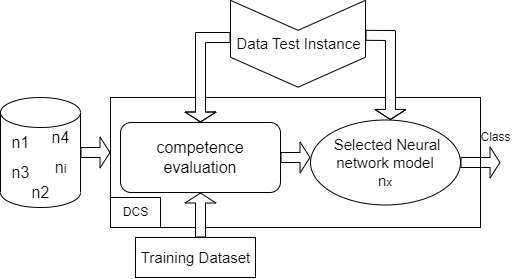
Figure 1: Diagram of dynamic classifier selection

In this adapted version of Dynamic Classifier Selection (DCS), the method incorporates k-Nearest Centroid for estimating model competence[20]. The feature space undergoes partitioning through the application of the k-means algorithm. Subsequent to this, every identified cluster is correspondingly linked to a neural network model, deemed most capable for the classification tasks pertinent to that specific cluster. Upon the introduction of a new test instance, an immediate assignment to its closest cluster occurs, followed by the invocation of the associated neural network model for the task of classification. This strategy, which centralizes around k-NC, optimally balances computational economy with classification precision.

II-B design of Competence Evaluation module

The architecture of our dynamic classifier selection is predicated on an efficient k-Nearest Centroid (k-NC) implementation. Figure 2 elucidates the essential elements of this architecture: Centroid Read-Only Memory (ROM), Distance Modules (DM), Control Unit and Comparator.

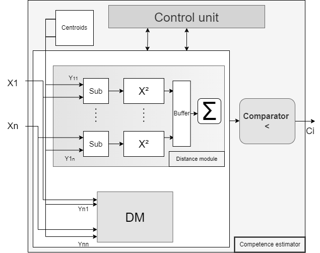
Figure 2: Diagram of the competence estimator

Within each DM, subtractors work in parallel, along with a multiplier and an accumulator. These components are optimized for rapid distance computations between an input data vector and pre-stored centroids.

The subtractors within a single DM function in parallel, generating the deltas between individual features of the input vector and those of a given centroid. Subsequently, a multiplier squares these differences these differences. An accumulator sums these products, thereby calculating the Euclidean distance pertaining to that centroid. The Euclidean distance is essentially calculated using the equation.

$$d(x,C)=\sqrt{\sum_{i=1}^{n}(x_{i}-C_{i})^{2}}$$ (1)

where $\mathbf{xi}$ and $\mathbf{Ci}$ are the individual features of the input vector and centroid.

the Control Unit stands as a crucial element. This unit exercises control over both data and computational activities. Given the limited number of just two Data Modules (DMs), the Control Unit governs multiple cycles to evaluate the full set of available centroids in relation to the input vector. The unit assumes the duty of reassigning centroids to DMs and ensures both temporal alignment and accurate data transfer among the various modules.

Upon the completion of centroid evaluation, the Control Unit channels the computed distances to a Distances Buffer for temporary storage. At this juncture, a Comparator queries the Distances Buffer to ascertain the least distance from among the calculated metrics. The Comparator then outputs the label associated with this minimal distance, thus determining the optimal accelerator for the processed input vector.

III The neural networks models design

In the devised neural network architecture, the emphasis is on creating a parameterized architecture that allows for a variable number of neurons and hidden layers, This design is particularly tailored to accommodate hidden layers that utilize Multiply-Accumulate (MAC) computations and Rectified Linear Unit (ReLU) activations.

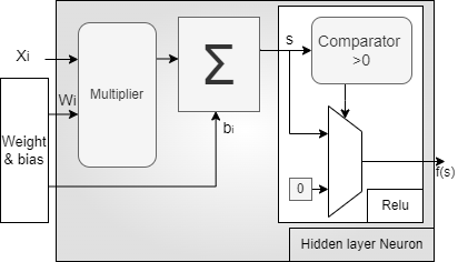
Figure 3: Diagram of the hidden layer neuron

In the implemented FPGA architecture, each neuron within the hidden layers is engineered to execute a Multiply-Accumulate (MAC) operation on its input vectors. As illustrated in Figure 3,the neurons utilize MAC operations for streamlined and efficient data processing.

In the formulated neural network architecture, the central aim is to provide for configurable numbers of neurons and hidden layers. The design is optimized to support hidden layers employing Multiply-Accumulate (MAC) operations as well as Rectified Linear Unit (ReLU) activation functions. Within the FPGA-based layout, each neuron in the hidden layers is precisely designed for executing a MAC operation on its array of input values. Specifically, the architecture adapts to computational demands, making it both flexible and efficient. the neuron multiplies each input element $\mathbf{X}$ with a corresponding weight $\mathbf{W}$ and subsequently adds a bias term $\mathbf{b}$, mathematically represented as

$$s=\sum_{i=1}^{n}w_{i}\cdot x_{i}+b$$ (2)

Following the execution of the Multiply-Accumulate (MAC) operation, the architecture incorporates a Rectified Linear Unit (ReLU) activation function to instill non-linearity into the neural model. In hardware terms, the ReLU functionality is achieved with utilization of a comparator and a 2:1 Multiplexer (MUX).The comparator’s output then directs the MUX to selectively pass either the original MAC output value or to default to zero, thereby effectuating the ReLU function. The comparator evaluates the MAC output $\mathbf{s}$ and generates a binary control signal. In mathematical terms, the ReLU is expressed as

$$y=\max(0,s)$$ (3)

In the architecture’s final output layer, the argmax function replaces the conventional softmax activation. This substitution is in line with our primary aim of improving classification accuracy, eliminating the need for a complete probability distribution among classes. The argmax function singles out the neuron with the highest output, efficiently converting it into a one-hot encoded vector. This optimized operation reduces computational load, thereby simplifying hardware deployment and speeding up the inference stage. The emphasis remains strictly on the measurement of system accuracy.

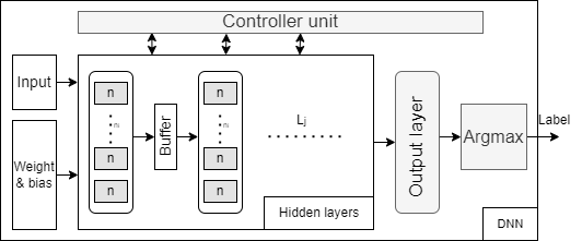
Figure 4: Diagram of the Neural network component

In Figure 4, the structural details of various neural network models within the ensemble are delineated. Each constituent model differs based on two fundamental hyperparameters: neuron count and layer count. This deliberate variance serves dual purposes. Primarily, it augments ensemble diversity, an essential element for the resilience of the Dynamic Classifier Selection (DCS) mechanism deployed on Field-Programmable Gate Arrays (FPGAs). Additionally, this heterogeneity is strategically designed to amplify system accuracy, constituting a substantial advantage over reliance on a singular neural network model. Equipped with a diverse ensemble of neural network models, the adaptative neural network possesses the capability to dynamically allocate the most suitable model for individual test instances.

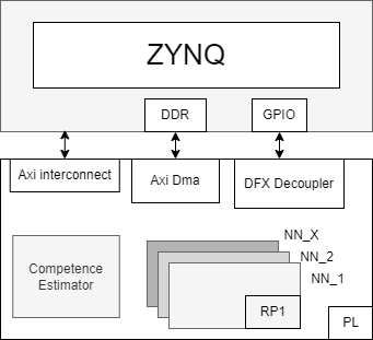
Figure 5: Diagram of the real-time Adaptive Neural Network Design

The foundation of our architecture is constituted by the Processing System (PS) incorporated into the Zynq System on Chip (SoC). As delineated in Figure 5,the PS is crucial in managing the operations of individual neural network modules as well as the competence estimator. This management is made possible due to the inherent high-performance, adaptability, and energy-efficient characteristics of Zynq platforms. Data transfer between our neural networks and competence estimator occurs via the AXI Direct Memory Access (DMA) and AXI Interconnect systems. The AXI DMA plays a vital role in facilitating efficient data migration between system memory and neural networks implementations, thereby minimizing CPU overhead and augmenting system efficacy. Furthermore, the AXI Interconnect operates using the AXI4-Lite protocol, which is instrumental in enabling the architecture to interpret output data from both the accelerators and the competence estimator. One feature of our architectural design is the incorporation of a Reconfigurable Partition (RP) region. Neural networks are situated within this RP area, interfacing with the FPGA through a Dynamic Function eXchange (DFX) decoupler. Control over the DFX decoupler is exerted by an GPIO, offering logical partitioning between static and RP areas during the reconfiguration stage. This arrangement permits the unproblematic interchange of bitstreams while simultaneously maintaining system robustness.

IV Experimental Implementation and Analysis

IV-A Dataset and parameters

In the current research, the Dynamic Classifier Selection (DCS) system’s performance and adaptability, deployed on Field-Programmable Gate Arrays (FPGAs), undergo evaluation using three disparate datasets. Distinctive in their levels of complexity, these datasets also diverge in their categorization tasks: one is oriented toward multiclass challenges and the other two focus on binary classification. Consistency in methodology is maintained by adopting an 85-15 data partitioning scheme. Specifically, 85% of each dataset contributes to model training, with the remaining 15% set aside for evaluation. During data preparation, we split the training data into two distinct sets. The first set trained three neural network models, while the second was used the remaining two. Such a division aimed to increase the diversity in the ensemble set.

NN model	Lj(Vehicle)	Lj(Diabetes)	Lj(German Credit)
NN1	(18,18,10)	(5,3)	(7,7)
NN2	(30,30,20)	(3,3)	(7,7,4)
NN3	(27,27,22)	(12,12,8)	(4,4)
NN4	(20,20,15)	(8,8,4)	(8,8,4)
NN5	(20,20,16)	(6,4,4)	(6,6,4)

TABLE I: Neural Network Model Parameters Utilized

Table I presents the customized neural network models for each of the three respective datasets, focusing on distinctions in the number of neurons and architectural layers. In the performance evaluation module of the architecture, the optimal centroid count is contingent upon the particular dataset under consideration. For the Vehicle Silhouette and German Credit datasets, an optimal configuration involves 70 centroids. Conversely, the Diabetes dataset demonstrates optimal performance with a centroid count of 50. These dataset-specific centroid counts are integral for fine-tuning the competence estimator module.

IV-B Ressource utilization

Resource utilization stands as a pivotal metric in evaluating the efficiency of the dynamic architecture designed for Field-Programmable Gate Arrays (FPGAs). In this analytical endeavor, we closely examine the resources consumed by each of the five neural network models of the vehicle data and the competence estimator.

NN models	LUTs	FFs	DSPs	BRAMs
NN1	4159	4658	100	0
NN2	6666	7137	168	0
NN3	6428	6849	160	0
NN4	4820	5309	118	0
NN5	4849	5381	120	0
C.E.	2958	6335	50	7

TABLE II: Comparison of resources used by various neural networks

For a more exhaustive evaluation, a hypothetical scenario is also considered, wherein a static architecture is employed, and all neural network models are implemented concurrently.

Resource	Static Implementation	Dynamic Implementation
LUTs	45397 (64.34%)	14224 (20.16%)
FFs	49006 (34.73%)	17265 (12.23%)
DSPs	716 (198.89%)	210 (58.33%)
BRAMs	13 (6.02%)	8 (3.70%)

TABLE III: Resource utilization: Comparison between Static and Dynamic Architectures

This resource evaluation is executed on the Ultra96-V2 Board, which constitutes the hardware basis of our dynamic architecture. By contrasting resource utilization in both dynamic and static configurations, the objective is to quantify the efficiency improvements attributable to the dynamic approach. Such an assessment is of particular importance in the context of FPGA deployments, where resource optimization is integral to achieving both high performance and cost efficiency. Through this analysis, the aim is to corroborate the resource efficiency of the dynamic architecture, Resource utilization was notably minimized, up to a factor of 109.28%, thereby affirming its applicability that demand computational efficiency.

V Results

Following an in-depth exploration of parameter tuning, specifically concerning the number of centroids for the competence estimator and the configurations of hidden layers in the neural network models, we now pivot to the results. This subsequent analysis leverages the optimized parameters to provide a quantitative assessment of the real-time adaptive neural network.

Figure 6: Performance evaluation for german credit dataset

Figure 7: Performance evaluation for diabetes dataset

Figure 8: Performance evaluation for vehicle dataset

Figures 6, 7, and 8 provide a numerical evaluation that contrasts the real-time adaptive neural network, a DCS-based architecture, with each of the ensemble’s individual neural network models. In the German Credit dataset, the architecture attains an 84.66% accuracy, outclassing the most effective individual model, which lags at 76.66%, thereby yielding an 8% improvement. For the Diabetes dataset, the architecture notches an 87.06% accuracy, surpassing the leading individual model, which registers at 82.75%. Finally, concerning the Vehicle Silhouette dataset, the architecture achieves a 94.48% accuracy, significantly better than the top-scoring individual model at 88.97%.

VI Conclusion

In conclusion, the present study conducts an exhaustive assessment of a real-time, adaptive neural network employing a DCS-based structural framework, tested across three varied datasets. Through parameter optimization, the architecture consistently surpassed the performance of individual ensemble models in classification accuracy metrics. Resource expenditure was notably minimized, up to a factor of 109.28%, via partial reconfiguration as opposed to a static implementation strategy.The findings serve to substantiate not only the high performance of the architecture but also its viable application in contexts necessitating a balance between accuracy and resource efficiency.

References

- [1] M. Bramer and M. Bramer, “An introduction to neural networks,” Principles of Data Mining, pp. 427–466, 2020.
- [2] R. Y. Choi, A. S. Coyner, J. Kalpathy-Cramer, M. F. Chiang, and J. P. Campbell, “Introduction to machine learning, neural networks, and deep learning,” Translational vision science & technology, vol. 9, no. 2, pp. 14–14, 2020.
- [3] M. Tkáč and R. Verner, “Artificial neural networks in business: Two decades of research,” Applied Soft Computing, vol. 38, pp. 788–804, 2016.
- [4] A. P. Marugán, F. P. G. Márquez, J. M. P. Perez, and D. Ruiz-Hernández, “A survey of artificial neural network in wind energy systems,” Applied energy, vol. 228, pp. 1822–1836, 2018.
- [5] N. Shahid, T. Rappon, and W. Berta, “Applications of artificial neural networks in health care organizational decision-making: A scoping review,” PloS one, vol. 14, no. 2, p. e0212356, 2019.
- [6] O. I. Abiodun, A. Jantan, A. E. Omolara, K. V. Dada, N. A. Mohamed, and H. Arshad, “State-of-the-art in artificial neural network applications: A survey,” Heliyon, vol. 4, no. 11, 2018.
- [7] P. Dhilleswararao, S. Boppu, M. S. Manikandan, and L. R. Cenkeramaddi, “Efficient hardware architectures for accelerating deep neural networks: Survey,” IEEE Access, 2022.
- [8] M. P. Véstias, “A survey of convolutional neural networks on edge with reconfigurable computing,” Algorithms, vol. 12, no. 8, p. 154, 2019.
- [9] C. Wang, W. Lou, L. Gong, L. Jin, L. Tan, Y. Hu, X. Li, and X. Zhou, “Reconfigurable hardware accelerators: Opportunities, trends, and challenges,” arXiv preprint arXiv:1712.04771, 2017.
- [10] K. P. Seng, P. J. Lee, and L. M. Ang, “Embedded intelligence on fpga: Survey, applications and challenges,” Electronics, vol. 10, no. 8, p. 895, 2021.
- [11] B. Seyoum, M. Pagani, A. Biondi, S. Balleri, and G. Buttazzo, “Spatio-temporal optimization of deep neural networks for reconfigurable fpga socs,” IEEE Transactions on Computers, vol. 70, no. 11, pp. 1988–2000, 2020.
- [12] K. Vipin and S. A. Fahmy, “Fpga dynamic and partial reconfiguration: A survey of architectures, methods, and applications,” ACM Computing Surveys (CSUR), vol. 51, no. 4, pp. 1–39, 2018.
- [13] K. Shi, M. Wang, X. Tan, Q. Li, and T. Lei, “Efficient dynamic reconfigurable cnn accelerator for edge intelligence computing on fpga,” Information, vol. 14, no. 3, p. 194, 2023.
- [14] K. Khalil, A. Kumar, and M. Bayoumi, “Reconfigurable hardware design approach for economic neural network,” IEEE Transactions on Circuits and Systems II: Express Briefs, vol. 69, no. 12, pp. 5094–5098, 2022.
- [15] R. M. Cruz, R. Sabourin, and G. D. Cavalcanti, “Dynamic classifier selection: Recent advances and perspectives,” Information Fusion, vol. 41, pp. 195–216, 2018.
- [16] G. Giacinto and F. Roli, “Dynamic classifier selection,” in International Workshop on Multiple Classifier Systems, pp. 177–189, Springer, 2000.
- [17] J. Gama, I. Žliobaitė, A. Bifet, M. Pechenizkiy, and A. Bouchachia, “A survey on concept drift adaptation,” ACM computing surveys (CSUR), vol. 46, no. 4, pp. 1–37, 2014.
- [18] P. R. Almeida, L. S. Oliveira, A. S. Britto Jr, and R. Sabourin, “Adapting dynamic classifier selection for concept drift,” Expert Systems with Applications, vol. 104, pp. 67–85, 2018.
- [19] J. M. Johnson and T. M. Khoshgoftaar, “Survey on deep learning with class imbalance,” Journal of Big Data, vol. 6, no. 1, pp. 1–54, 2019.
- [20] R. G. Soares, A. Santana, A. M. Canuto, and M. C. P. de Souto, “Using accuracy and diversity to select classifiers to build ensembles,” in The 2006 IEEE International Joint Conference on Neural Network Proceedings, pp. 1310–1316, IEEE, 2006.