On the range of fractal interpolation functions

Abstract. In this paper, based on the results from [On the localization of Hutchinson–Barnsley fractals, Chaos Solitons Fractals, 173 (2023), 113674], we generate coverings (consisting of finite families of rhombi) of the graph of fractal interpolation functions. As a by-product we obtain estimations for the range of such functions. Some concrete examples and graphical representations are provided.

Keywords: iterated function system, fractal interpolation function, range of a function

MSC: 28A80, 41A05

1 Introduction

Fractal interpolation functions (abbreviated FIFs) are extremely useful instruments for modeling irregular patterns which produce smooth and non-smooth interpolants. They have been introduced by M. Barnsley, via the concept of iterated function system (see [11]), including and supplementing the classical interpolants. Following the seminal work of M. Barnsley (see [3]), the fractal interpolation functions theory has been expanded in several ways. For example:
- affine zipper fractal interpolation functions are considered in [5]
- vector valued fractal interpolation functions are treated in [18]
- local fractal interpolation functions are examined in [20]
- fractal interpolation functions with variable parameters are investigated in [33]
- graph-directed fractal interpolation functions are studied in [9]
- fractal interpolation functions with partial self similarity are explored in [15].
See also [21], [22], [25], [26], [28] and [31].

Some fields where one can find applications of FIFs encompass:
- signal analysis (see [2])
- satellite images (see [6])
- medicine (see [8] and [30])
- image compression (see [10])
- financial analysis (see [13])
- ecology (see [14])
- signal reconstruction (see [12], [23] and [36])
- geology (see [34])
- meteorology (see [35]).

Excellent surveys on fractal interpolation functions could be found in [2], [4], [19], [24] and [27].

The brusque oscillations occurring in fractal interpolation functions modeling financial data (which are of great interest for decision makers and investors see [16]) is a strong reason to study the range of a FIF. An additional motive, from the point of view of cardiologists, for such a study stems from [29]. Actually such an investigation, but in some particular cases, has been done in [7] and [32].

In this paper, based on the results from [1], we generate coverings (consisting of finite families of rhombi) of the graph of fractal interpolation functions (see Theorem 3.1). As a by-product we obtain estimations for the range of such functions (see Theorem 3.2). Some concrete examples and graphical representations are provided in the last section.

2 Preliminaries

Given a metric space $(X,d)$, $x\in X$ and $r>0$ we shall use the following notation:

• $B[x,r]=\{y\in X\;|\;d(y,x)\leq r\}$

• $\mathcal{P}_{cp}(X)=\{A\subseteq X|A\text{ is non-empty and compact}\}$

• $h$ is the Hausdorff-Pompeiu metric, described by

  $$h(K_{1},K_{2})=\max\left\{\sup_{x\in K_{1}}d(x,K_{2}),\sup_{x\in K_{2}}d(x,K_{1})\right\},$$

  for all $K_{1},K_{2}\in\mathcal{P}_{cp}(X)$.

For a Lipschitz function $f:X\to X$ we shall denote by $\text{Lip}(f)$ the Lipschitz constant of $f$.

Let us recall the following well known result:

Lemma 2.1.

Let $A_{1},\;A_{2},\dots,\;A_{n}$, where $n\in\mathbb{N}$, be non-empty, bounded subsets of $\mathbb{R}$. Then

$$\sup(A_{1}\cup A_{2}\cup\dots\cup A_{n})=\max\{\sup A_{1},\sup A_{2},\dots,\sup A_{n}\}.$$

Definition 2.1.

An iterated function system (for short IFS) is a pair $\mathcal{S}=((X,d),(f_{i})_{i\in I})$, where $(X,d)$ is a complete metric space and $f_{i}:X\to X$, $i\in I$, are Banach contractions.

The function $F_{\mathcal{S}}:\mathcal{P}_{cp}(X)\to\mathcal{P}_{cp}(X)$, given by

$$F_{\mathcal{S}}(K)=\bigcup_{i\in I}f_{i}(K),$$

for every $K\in\mathcal{P}_{cp}(X)$, is called the fractal operator (or the Hutchinson operator) associated with $\mathcal{S}$.

Proposition 2.1.

If $\mathcal{S}=((X,d),(f_{i})_{i\in I})$ is an iterated function system, then $F_{\mathcal{S}}$ is a contraction with respect to $h$. Its unique fixed point is denoted by $\mathcal{A}_{\mathcal{S}}$ and it is called the attractor of $\mathcal{S}$ since

$$\lim_{n\to\infty}\underbrace{(F_{\mathcal{S}}\circ F_{\mathcal{S}}\circ\dots\circ F_{\mathcal{S}})}_{n\text{ times }}(K)=\mathcal{A}_{\mathcal{S}},$$

for each $K\in\mathcal{P}_{cp}(X).$

Theorem 2.1 (see Theorem 3.1 from [1]).

For an iterated function system $\mathcal{S}=((X,d),(f_{i})_{i\in\{1,\dots n\}})$, we have

$$\mathcal{A}_{\mathcal{S}}\subseteq\left(\bigcup_{i\in\{1,\dots,\;n-1\}}B\left[\gamma_{i},Ms_{i}\frac{1+s_{n}}{1-s_{{n-1}}s_{n}}\right]\right)\bigcup B\left[\gamma_{n},Ms_{n}\frac{1+s_{{n-1}}}{1-s_{{n-1}}s_{n}}\right],$$

where

1. $s_{i}=\text{Lip}(f_{i})$ for each $i\in\{1,\dots,n\}$

2. $s_{1}\leq s_{2}\leq\dots\leq s_{n}$

3. $\gamma_{i}$ is the unique fixed point of $f_{i}$ for each $i\in\{1,\dots,n\}$

4. $M=\max_{i,j\in\{1,\dots,n\}}d(\gamma_{i},\gamma_{j})$.

3 The main results

The framework of our main result

Inspired by [3] and [4], let $n\in\mathbb{N}$ and $(x_{0},y_{0}),(x_{1},y_{1}),\dots,(x_{n},y_{n})\in\mathbb{R}^{2}$ with

$$a:=x_{0}<x_{1}<\dots<x_{n}=:b$$

and let us consider the iterated function system $\mathcal{S}=((\mathbb{R}^{2},\rho),(f_{k})_{k\in\{1,\dots,n\}})$, where:

• $f_{k}:\mathbb{R}^{2}\to\mathbb{R}$ is given by

  $$f_{k}(x,y)=(a_{k}x+b_{k},c_{k}x+d_{k}y+e_{k}),$$

  for all $(x,y)\in\mathbb{R}^{2}$ and $k\in\{1,\dots,n\}$, where

  $$a_{k} =\frac{x_{k}-x_{k-1}}{x_{n}-x_{0}}$$

  $$b_{k} =\frac{x_{n}x_{k-1}-x_{0}x_{k}}{x_{n}-x_{0}}$$

  $$d_{k} \in[0,1)$$

  $$c_{k} =\frac{y_{k}-y_{k-1}}{x_{n}-x_{0}}-d_{k}\frac{y_{n}-y_{0}}{x_{n}-x_{0}}$$

  $$e_{k} =\frac{x_{n}y_{k-1}-x_{0}y_{k}}{x_{n}-x_{0}}-d_{k}\frac{x_{n}y_{0}-x_{0}y_{n}}{x_{n}-x_{0}};$$

• the complete metric $\rho:\mathbb{R}^{2}\times\mathbb{R}^{2}\to[0,\infty)$ is given by

  $$\rho((u_{1},v_{1}),(u_{2},v_{2}))=|u_{1}-u_{2}|+\theta|v_{1}-v_{2}|,$$

  for all $(u_{1},v_{1}),(u_{2},v_{2})\in\mathbb{R}^{2}$, where

  $$\theta=\left\{\begin{aligned} &1,&&c_{1}=c_{2}=\dots=c_{n}=0;\\ &\frac{1-\max_{k\in\{1\dots n\}}a_{k}}{2\max_{k\in\{1,\dots,n\}}|c_{k}|},&&\text{otherwise}.\end{aligned}\right.$$

Then, there exists a continuous function $f:[a,b]\to\mathbb{R}$, which is called an affine fractal interpolation function, such that :

• $$f(x_{k})=y_{k},$$

  for all $k\in\{0,1,\dots,n\}$

• $$G_{f}=\mathcal{A}_{\mathcal{S}}.$$

Finding the fixed point of $f_{k}$

For a fixed, but arbitrarily chosen $k\in\{1,\dots,n\}$, from $f_{k}(\gamma_{k})=\gamma_{k}=(u_{k},v_{k})$ we obtain

$$(a_{k}u_{k}+b_{k},c_{k}u_{k}+d_{k}v_{k}+e_{k})=(u_{k},v_{k}),$$

hence

$$\begin{cases}a_{k}u_{k}+b_{k}&=u_{k}\\ c_{k}u_{k}+d_{k}v_{k}+e_{k}&=v_{k}.\end{cases}$$

From the first equation, we deduce that

$$u_{k}=\frac{b_{k}}{1-a_{k}}.$$

Substituting in the second equation, we obtain

$$c_{k}\frac{b_{k}}{1-a_{k}}+d_{k}v_{k}+e_{k}=v_{k},$$

so

$$v_{k}=\frac{b_{k}c_{k}}{(1-a_{k})(1-d_{k})}+\frac{e_{k}}{1-d_{k}}.$$

Hence, the (unique) fixed point of $f_{k}$ is

$$\gamma_{k}=\left(\frac{b_{k}}{1-a_{k}},\frac{b_{k}c_{k}}{(1-a_{k})(1-d_{k})}+\frac{e_{k}}{1-d_{k}}\right),$$

for all $k\in\{1,\dots,n\}$.

Finding the Lipschitz constant of $f_{k}$

Proposition 3.1.

In the above mentioned framework, we have

$$\text{Lip}(f_{k})=\max\{d_{k},a_{k}+\theta|c_{k}|\},$$

for every $k\in\{1,\dots,n\}$

Proof.

Let us consider $k\in\{1,\dots,n\}$ arbitrarily chosen, but fixed.

Note that

$$\text{Lip}(f_{k})=\sup\mathcal{M},$$

where

$$\mathcal{M}= \left\{\frac{\rho\bm{(}f_{k}(u_{1},v_{1}),f_{k}(u_{2},v_{2})\bm{)}}{\rho\bm{(}(u_{1},v_{1}),(u_{2},v_{2})\bm{)}}\big{|}{(u_{1},v_{1}),(u_{2},v_{2})\in\mathbb{R}^{2},(u_{1},v_{1})\neq(u_{2},v_{2})}\right\}$$

$$= \left\{\frac{a_{k}|u_{1}-u_{2}|+\theta|c_{k}(u_{1}-u_{2})+d_{k}(v_{1}-v_{2})|}{|u_{1}-u_{2}|+\theta|v_{1}-v_{2}|}\big{|}{(u_{1},v_{1}),(u_{2},v_{2})\in\mathbb{R}^{2},(u_{1},v_{1})\neq(u_{2},v_{2})}\right\}.$$

If $d_{k}=0$, we get

$$\mathcal{M}= \left\{\frac{a_{k}|u_{1}-u_{2}|+\theta|c_{k}(u_{1}-u_{2})|}{|u_{1}-u_{2}|+\theta|v_{1}-v_{2}|}\big{|}{(u_{1},v_{1}),(u_{2},v_{2})\in\mathbb{R}^{2},v_{1}\neq v_{2},u_{1}=u_{2}}\right\}$$

$$\qquad\bigcup\left\{\frac{a_{k}|u_{1}-u_{2}|+\theta|c_{k}(u_{1}-u_{2})|}{|u_{1}-u_{2}|+\theta|v_{1}-v_{2}|}\big{|}(u_{1},v_{1}),(u_{2},v_{2})\in\mathbb{R}^{2},u_{1}\neq u_{2}\right\}$$

$$= \{0\}\cup\left\{\frac{(a_{k}+\theta|c_{k}|)|u_{1}-u_{2}|}{|u_{1}-u_{2}|+\theta\left|v_{1}-v_{2}\right|}\big{|}(u_{1},v_{1}),(u_{2},v_{2})\in\mathbb{R}^{2},u_{1}\neq u_{2}\right\}$$

$$= \{0\}\cup\left\{\frac{a_{k}+\theta|c_{k}|}{1+\theta\left|\frac{v_{1}-v_{2}}{u_{1}-u_{2}}\right|}\big{|}(u_{1},v_{1}),(u_{2},v_{2})\in\mathbb{R}^{2},u_{1}\neq u_{2}\right\}$$

$$= \{0\}\cup\left\{\frac{a_{k}+\theta|c_{k}|}{1+\theta\left|t\right|}\big{|}t\in\mathbb{R}\right\}.$$

Since

$$\sup\left\{\frac{a_{k}+\theta|c_{k}|}{1+\theta\left|t\right|}\big{|}t\in\mathbb{R}\right\}=a_{k}+\theta|c_{k}|,$$

taking into account Lemma 2.1, we get

$$\text{Lip}(f_{k})=\max\{0,a_{k}+\theta|c_{k}|\}=\max\{d_{k},a_{k}+\theta c_{k}\}.$$

So, we can suppose that $d_{k}>0$.

We have

$$\mathcal{M}= \left\{\frac{a_{k}|u_{1}-u_{2}|+\theta|c_{k}(u_{1}-u_{2})+d_{k}(v_{1}-v_{2})|}{|u_{1}-u_{2}|+\theta|v_{1}-v_{2}|}\big{|}{(u_{1},v_{1}),(u_{2},v_{2})\in\mathbb{R}^{2},v_{1}\neq v_{2},u_{1}=u_{2}}\right\}$$

$$\qquad\bigcup\left\{\frac{a_{k}|u_{1}-u_{2}|+\theta|c_{k}(u_{1}-u_{2})+d_{k}(v_{1}-v_{2})|}{|u_{1}-u_{2}|+\theta|v_{1}-v_{2}|}\big{|}(u_{1},v_{1}),(u_{2},v_{2})\in\mathbb{R}^{2},u_{1}\neq u_{2}\right\}$$

$$= \{d_{k}\}\cup\left\{\frac{a_{k}|u_{1}-u_{2}|+\theta|c_{k}(u_{1}-u_{2})+d_{k}(v_{1}-v_{2})|}{|u_{1}-u_{2}|+\theta\left|v_{1}-v_{2}\right|}\big{|}(u_{1},v_{1}),(u_{2},v_{2})\in\mathbb{R}^{2},u_{1}\neq u_{2}\right\}$$

$$= \{d_{k}\}\cup\left\{\frac{a_{k}+\theta|c_{k}+d_{k}\frac{v_{1}-v_{2}}{u_{1}-u_{2}}|}{1+\theta\left|\frac{v_{1}-v_{2}}{u_{1}-u_{2}}\right|}\big{|}(u_{1},v_{1}),(u_{2},v_{2})\in\mathbb{R}^{2},u_{1}\neq u_{2}\right\}$$

$$= \{d_{k}\}\cup\left\{\frac{a_{k}+\theta|c_{k}+d_{k}t|}{1+\theta\left|t\right|}\big{|}t\in\mathbb{R}\right\}.$$

We divide our proof in three cases, namely:

1. Case 1. $c_{k}=0$

2. Case 2. $c_{k}<0$

3. Case 3. $c_{k}>0$

In the first case, we have

$$\mathcal{M}=\{d_{k}\}\cup\left\{\frac{a_{k}+\theta d_{k}x}{1+\theta x}\big{|}x\geq 0\right\}.$$

Since

$$\sup\left\{\frac{a_{k}+\theta d_{k}x}{1+\theta x}\big{|}x\geq 0\right\}=\begin{cases}d_{k},&\qquad d_{k}\geq a_{k}\\ a_{k}=a_{k}+\theta|c_{k}|,&\qquad d_{k}<a_{k}\end{cases},$$

via Lemma 2.1, we get

$$\text{Lip}(f_{k})=\sup\mathcal{M}=\max\{d_{k},a_{k}+\theta|c_{k}|\}.$$

In the second case, we have

$$\mathcal{M}=\{d_{k}\}\cup\mathcal{M}_{1}\cup\mathcal{M}_{2}\cup\mathcal{M}_{3},$$

where

$$\mathcal{M}_{1} =\left\{\frac{a_{k}+\theta c_{k}+\theta d_{k}t}{1+\theta t}\big{|}t\geq-\frac{c_{k}}{d_{k}}\right\},$$

$$\mathcal{M}_{2} =\left\{\frac{a_{k}-\theta c_{k}-\theta d_{k}t}{1+\theta t}\big{|}0<t<-\frac{c_{k}}{d_{k}}\right\}$$

and

$$\mathcal{M}_{3} =\left\{\frac{a_{k}-\theta c_{k}-\theta d_{k}t}{1-\theta t}\big{|}t\leq 0\right\}.$$

Studying the monotonicity of the expressions that define the sets $\mathcal{M}_{1}$, $\mathcal{M}_{2}$ and $\mathcal{M}_{3}$, we infer that

$$\sup\mathcal{M}_{1} =\begin{cases}d_{k},&\qquad a_{k}+\theta c_{k}\leq d_{k}\\ \frac{a_{k}d_{k}}{d_{k}-\theta c_{k}},&\qquad a_{k}+\theta c_{k}>d_{k}\end{cases},$$

$$\sup\mathcal{M}_{2} =a_{k}-\theta c_{k}=a_{k}+\theta|c_{k}|$$

and

$$\sup\mathcal{M}_{3} =\begin{cases}a_{k}-\theta c_{k}=a_{k}+\theta|c_{k}|,&\qquad a_{k}-\theta c_{k}>d_{k}\\ d_{k},&\qquad a_{k}-\theta c_{k}\leq d_{k}\end{cases}.$$

Based on Lemma 2.1, we get

$$\text{Lip}(f_{k})=\sup\mathcal{M}=\max\{d_{k},\sup\mathcal{M}_{1},\sup\mathcal{M}_{2},\sup\mathcal{M}_{3}\},$$

hence

$$\text{Lip}(f_{k})=\max\{d_{k},a_{k}+\theta|c_{k}|,\sup\mathcal{M}_{1},\sup\mathcal{M}_{3}\}.$$ (3.1)

Further, we divide our discussion into three subcases, specifically:

1. $d_{k}<a_{k}+\theta c_{k}$

2. $a_{k}+\theta c_{k}\leq d_{k}<a_{k}-\theta c_{k}$

3. $a_{k}-\theta c_{k}\leq d_{k}$.

Note that in case $(\alpha)$ we have $d_{k}<a_{k}+\theta c_{k}<a_{k}-\theta c_{k}$ and in case $(\gamma)$ we have $a_{k}+\theta c_{k}<a_{k}-\theta c_{k}\leq d_{k}$.

In case $(\alpha)$, (3.1) yields

$$\text{Lip}(f_{k})=\max\left\{d_{k},a_{k}+\theta|c_{k}|,\frac{a_{k}d_{k}}{d_{k}-\theta c_{k}}\right\}=\max\{d_{k},a_{k}+\theta|c_{k}|\},$$

since

$$\frac{a_{k}d_{k}}{d_{k}-\theta c_{k}}\leq a_{k}+\theta|c_{k}|.$$

In cases $(\beta)$ and $(\gamma)$, via (3.1), we get

$$\text{Lip}(f_{k})=\max\left\{d_{k},a_{k}+\theta|c_{k}|\right\}.$$

In the third case, we have

$$\mathcal{M}=\{d_{k}\}\cup\mathcal{N}_{1}\cup\mathcal{N}_{2}\cup\mathcal{N}_{3},$$

where

$$\mathcal{N}_{1} =\left\{\frac{a_{k}+\theta c_{k}+\theta d_{k}t}{1+\theta t}\big{|}t\geq 0\right\},$$

$$\mathcal{N}_{2} =\left\{\frac{a_{k}+\theta c_{k}+\theta d_{k}t}{1-\theta t}\big{|}-\frac{c_{k}}{d_{k}}<t<0\right\}$$

and

$$\mathcal{N}_{3} =\left\{\frac{a_{k}-\theta c_{k}-\theta d_{k}t}{1-\theta t}\big{|}t\leq-\frac{c_{k}}{d_{k}}\right\}.$$

Since

$$\sup\mathcal{N}_{1} =\begin{cases}d_{k},&\qquad a_{k}+\theta c_{k}\leq d_{k}\\ a_{k}+\theta c_{k}=a_{k}+\theta|c_{k}|,&\qquad a_{k}+\theta c_{k}>d_{k}\end{cases},$$

$$\sup\mathcal{N}_{2} =a_{k}+\theta c_{k}=a_{k}+\theta|c_{k}|$$

and

$$\sup\mathcal{N}_{3} =\begin{cases}\frac{a_{k}d_{k}}{d_{k}+\theta c_{k}},&\qquad a_{k}-\theta c_{k}>d_{k}\\ d_{k},&\qquad a_{k}-\theta c_{k}\leq d_{k}\end{cases},$$

based on Lemma 2.1, we obtain

$$\text{Lip}(f_{k})=\sup\mathcal{M}=\max\{d_{k},\sup\mathcal{N}_{1},\sup\mathcal{N}_{2},\sup\mathcal{N}_{3}\},$$

hence

$$\text{Lip}(f_{k})=\max\{d_{k},a_{k}+\theta|c_{k}|,\sup\mathcal{N}_{1},\sup\mathcal{N}_{3}\}.$$ (3.2)

Further, we divide our discussion into three subcases, specifically:

1. $d_{k}<a_{k}-\theta c_{k}$

2. $a_{k}-\theta c_{k}\leq d_{k}<a_{k}+\theta c_{k}$

3. $a_{k}+\theta c_{k}\leq d_{k}$.

Note that in case $(\alpha)$ we have $d_{k}<a_{k}-\theta c_{k}<a_{k}+\theta c_{k}$ and in case $(\gamma)$ we have $a_{k}-\theta c_{k}<a_{k}+\theta c_{k}\leq d_{k}$.

In case $(\alpha)$, (3.2) ensures

$$\text{Lip}(f_{k})=\max\left\{d_{k},a_{k}+\theta|c_{k}|,\frac{a_{k}d_{k}}{d_{k}+\theta c_{k}}\right\}=\max\{d_{k},a_{k}+\theta|c_{k}|\},$$

since

$$\frac{a_{k}d_{k}}{d_{k}+\theta c_{k}}\leq a_{k}+\theta|c_{k}|.$$

In cases $(\beta)$ and $(\gamma)$, via (3.2), we get

$$\text{Lip}(f_{k})=\max\left\{d_{k},a_{k}+\theta|c_{k}|\right\}.$$

All in all, we obtain

$$\text{Lip}(f_{k})=\max\left\{d_{k},a_{k}+\theta|c_{k}|\right\}.$$

∎

Remark 3.1.

In view of the choice of $d_{k}$ and $\theta$, we have

$$\text{Lip}(f_{k})<1,$$

for all $k\in\{1,\dots,n\}$.

Describing the balls with respect to the metric $\rho$

For $r\geq 0$ and $(x,y)\in\mathbb{R}^{2}$, the closed ball with center $(x,y)$ and radius $r$, with respect to $\rho$, is the set

$$\{ (u,v)\in\mathbb{R}^{2}|\rho\bm{(}(x,y),(u,v)\bm{)}\leq r\} =\{(u,v)\in\mathbb{R}^{2}||x-u|+\theta|y-v|\leq r\}=:R[(x,y),r],$$

whose border is the rhombus having the vertixes $V_{1}\left(x+r,y\right)$, $V_{2}\left(x-r,y\right)$, $V_{3}\left(x,y+\frac{r}{\theta}\right)$ and $V_{4}\left(x,y-\frac{r}{\theta}\right).$

Remark 3.2.

Note that

$$\max\{v\in\mathbb{R}|\text{ there exists }u\in\mathbb{R}\text{ such that }(u,v)\in R[(x,y),r]\}=y+\frac{r}{\theta}$$

and

$$\min\{v\in\mathbb{R}|\text{ there exists }u\in\mathbb{R}\text{ such that }(u,v)\in R[(x,y),r]\}=y-\frac{r}{\theta}.$$

Obtaining a cover for $G_{f}$

Summing up, in the previous framework, via Theorem 2.1, by relabeling the functions $f_{k}$ such that $s_{1}\leq s_{2}\leq\dots\leq s_{n}$, we get the following result:

Theorem 3.1.

$$G_{f}\subseteq\left(\bigcup_{k\in\{1,\dots,\;n-1\}}R\left[\gamma_{k},Ms_{k}\frac{1+s_{n}}{1-s_{{n-1}}s_{n}}\right]\right)\bigcup R\left[\gamma_{n},Ms_{n}\frac{1+s_{{n-1}}}{1-s_{{n-1}}s_{n}}\right],$$

where

$$\gamma_{k}=\left(\frac{b_{k}}{1-a_{k}},\frac{b_{k}c_{k}}{(1-a_{k})(1-d_{k})}+\frac{e_{k}}{1-d_{k}}\right),$$

$$s_{k}=\max\{a_{k}+\theta|c_{k}|,d_{k}\},$$

for all $k\in\{1,\dots,n\}$,

$$\theta=\left\{\begin{aligned} &1,&&c_{1}=c_{2}=\dots=c_{n}=0;\\ &\frac{1-\max_{k\in\{1\dots n\}}a_{k}}{2\max_{k\in\{1,\dots,n\}}|c_{k}|},&&\text{otherwise}\end{aligned}\right.$$

and

$$M=\max_{i,j\in\{1,\dots,n\}}\left\{\left|\frac{b_{i}}{1-a_{i}}-\frac{b_{j}}{1-a_{j}}\right|+\theta\left|\frac{c_{i}b_{i}}{(1-a_{i})(1-d_{i})}+\frac{e_{i}}{1-d_{i}}-\frac{c_{j}b_{j}}{(1-a_{j})(1-d_{j})}-\frac{e_{j}}{1-d_{j}}\right|\right\}.$$

The set

$$\mathcal{C_{\mathcal{S}}}:=\left(\bigcup_{k\in\{1,\dots,\;n-1\}}R\left[\gamma_{k},Ms_{k}\frac{1+s_{n}}{1-s_{{n-1}}s_{n}}\right]\right)\bigcup R\left[\gamma_{n},Ms_{n}\frac{1+s_{{n-1}}}{1-s_{{n-1}}s_{n}}\right]$$

will be called the covering of $G_{f}$ associated to the system $\mathcal{S}$. For $m\in\mathbb{N}$, we will denote

$$\mathcal{C}_{\mathcal{S}_{m}}=\mathcal{C}_{m},$$

where

$$\mathcal{S}_{m}=\left((\mathbb{R}^{2},\rho),(f_{k_{1}}\circ\dots\circ f_{k_{m}})_{k_{1},\dots,k_{m}\in\{1,\dots,n\}}\right).$$

Remark 3.3.

According to Theorem 3.2 from [1], by applying Theorem 3.1 for the IFSs $\mathcal{S}_{m}$, $m\in\mathbb{N}$, we obtain coverings of $G_{f}$ with balls having the radii as small as we want.

Let us note that, in view of Remark 3.2 from [1], we have

$$\lim_{m\to\infty}h(\mathcal{C}_{m},G_{f})=0.$$

Remark 3.4.

In the above mentioned framework, for $k_{1},k_{2},\dots k_{m}\in\{1,\dots,n\}$, with $m\in\mathbb{N}$, $m\geq 2$, we have

$$(f_{k_{1}}\circ\dots\circ f_{k_{m}})(x,y)=(a_{k_{1}k_{2}\dots k_{m}}x+b_{k_{1}k_{2}\dots k_{m}},c_{k_{1}k_{2},\dots k_{m}}x+d_{k_{1}k_{2},\dots k_{m}}y+e_{k_{1}k_{2}\dots k_{m}}),$$

for all $x,y\in\mathbb{R}$, where $a_{k_{1}k_{2}\dots k_{m}}$, $b_{k_{1}k_{2}\dots k_{m}}$, $c_{k_{1}k_{2}\dots k_{m}}$ , $d_{k_{1}k_{2}\dots k_{m}}$ and $e_{k_{1}k_{2}\dots k_{m}}$ can be obtained recursively from the following formulas

$$\left\{\begin{aligned} a_{k_{1}k_{2}\dots k_{m}}&=a_{k_{1}}a_{k_{2}\dots k_{m}}\\ b_{k_{1}k_{2}\dots k_{m}}&=a_{k_{1}}b_{k_{2}\dots k_{m}}+b_{k_{1}}\\ c_{k_{1}k_{2}\dots k_{m}}&=c_{k_{1}}a_{k_{2}\dots k_{m}}+d_{k_{1}}c_{k_{2}k_{3}\dots k_{m}}\\ d_{k_{1}k_{2}\dots k_{m}}&=d_{k_{1}}d_{k_{2}\dots k_{m}}\\ e_{k_{1}k_{2}\dots k_{m}}&=c_{k_{1}}b_{k_{2}\dots k_{m}}+d_{k_{1}}e_{k_{2}\dots k_{m}}+e_{k_{1}},\end{aligned}\right.$$

which represent a very good tool for improving the efficiency of the computations involved.

Obtaining an estimation for $Imf$

Based on Remark 3.2 and Theorem 3.1, we obtain the following result:

Theorem 3.2.

In the previous framework, we have:

$$Imf\subseteq[A,B],$$

where

$$A=\min \left\{\min_{k\in\{1,\dots,n-1\}}\left(\frac{b_{k}c_{k}}{(1-a_{k})(1-d_{k})}+\frac{e_{k}}{1-d_{k}}-\frac{Ms_{k}(1+s_{n})}{\theta(1-s_{n-1}s_{n})}\right),\right.$$

$$\left.\frac{b_{n}c_{n}}{(1-a_{n})(1-d_{n})}+\frac{e_{n}}{1-d_{n}}-\frac{Ms_{n}(1+s_{n-1})}{\theta(1-s_{n-1}s_{n})}\right\}$$

and

$$B=\max \left\{\max_{k\in\{1,\dots,n-1\}}\left(\frac{b_{k}c_{k}}{(1-a_{k})(1-d_{k})}+\frac{e_{k}}{1-d_{k}}+\frac{Ms_{k}(1+s_{n})}{\theta(1-s_{n-1}s_{n})}\right),\right.$$

$$\left.\frac{b_{n}c_{n}}{(1-a_{n})(1-d_{n})}+\frac{e_{n}}{1-d_{n}}+\frac{Ms_{n}(1+s_{n-1})}{\theta(1-s_{n-1}s_{n})}\right\}.$$

Corollary 3.1.

In the previous framework, we have

$$G_{f}\subseteq[a,b]\times[A,B].$$

Remark 3.5.

Note that, $A$ and $B$ can be algebraically expressed in terms of the data set $(x_{0},y_{0})$,  $(x_{1},y_{1}),\dots$, $(x_{n},y_{n})$ and the scaling factors $d_{k}$.

4 Examples

We are going to apply our results for the following frameworks (which are considered in [17], [16] and respectively [12]):

Framework 1

• the data set is

  $\{(0,3),(1,2),(2,4),(3,3),(4,4)\}$

• $d_{k}=\frac{3}{10},$

for each $k\in\{1,2,3,4\}$.

The pictures $F_{11},F_{12},F_{13},F_{14}$ and $F_{15}$ contain the graphical representations of $\mathcal{C}_{1}$, $\mathcal{C}_{2}$, $\mathcal{C}_{3}$, $\mathcal{C}_{4}$ and respectively $\mathcal{C}_{5}$.

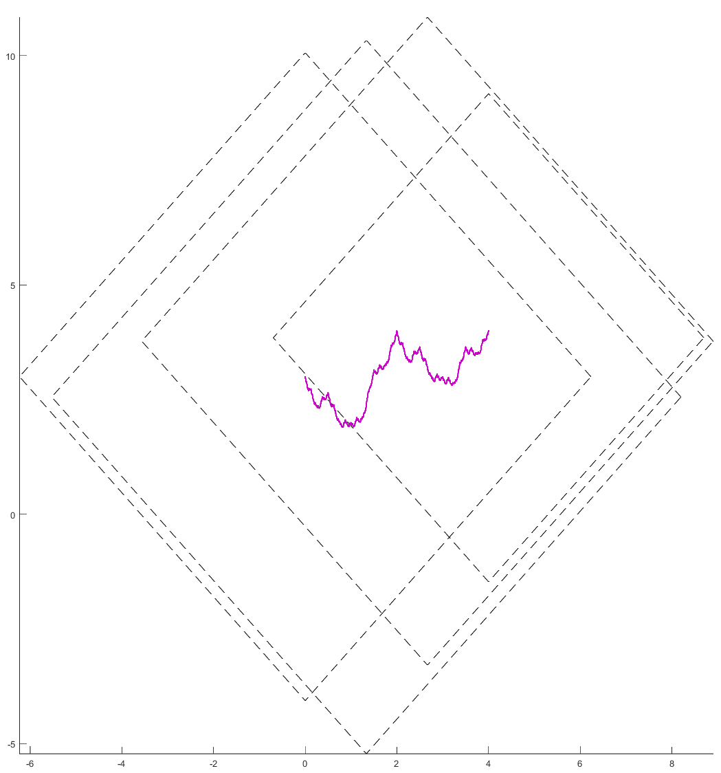
(a) $F_{11}:$ Visualization of $\mathcal{C}_{1}$

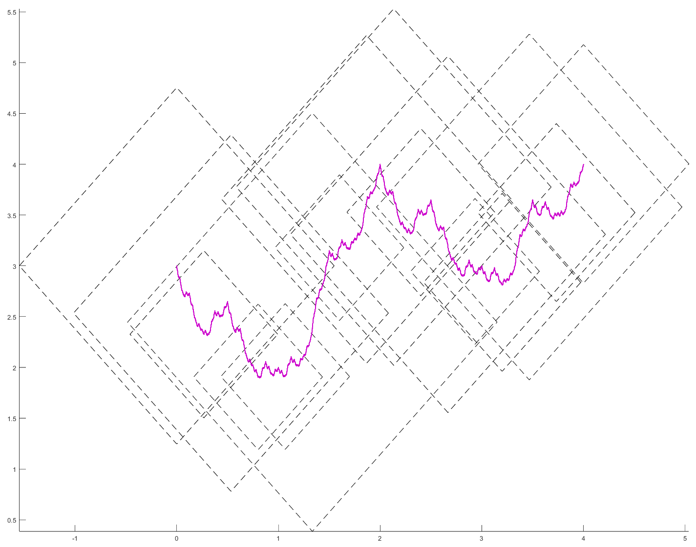
(b) $F_{12}:$ Visualization of $\mathcal{C}_{2}$

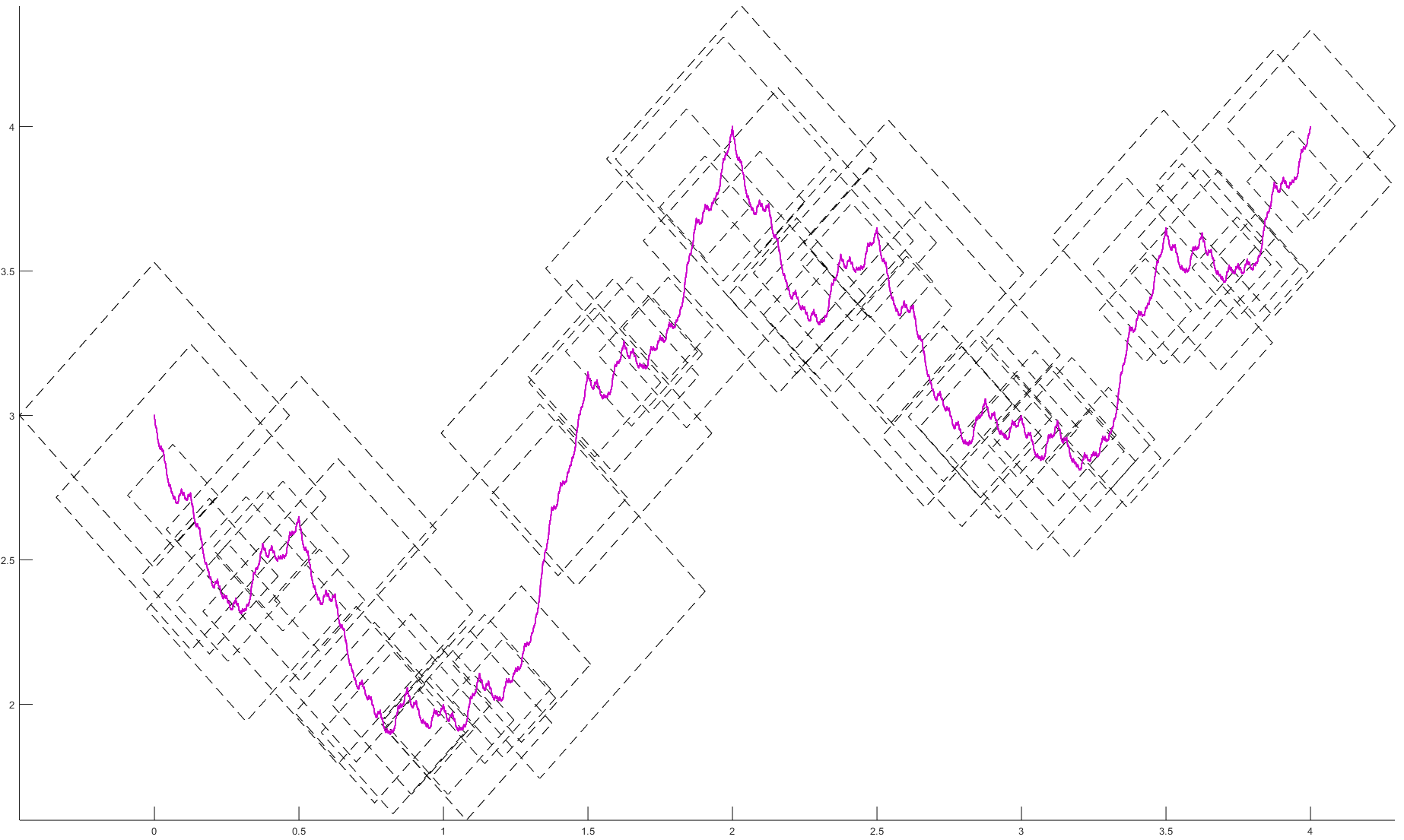
(c) $F_{13}:$ Visualization of $\mathcal{C}_{3}$

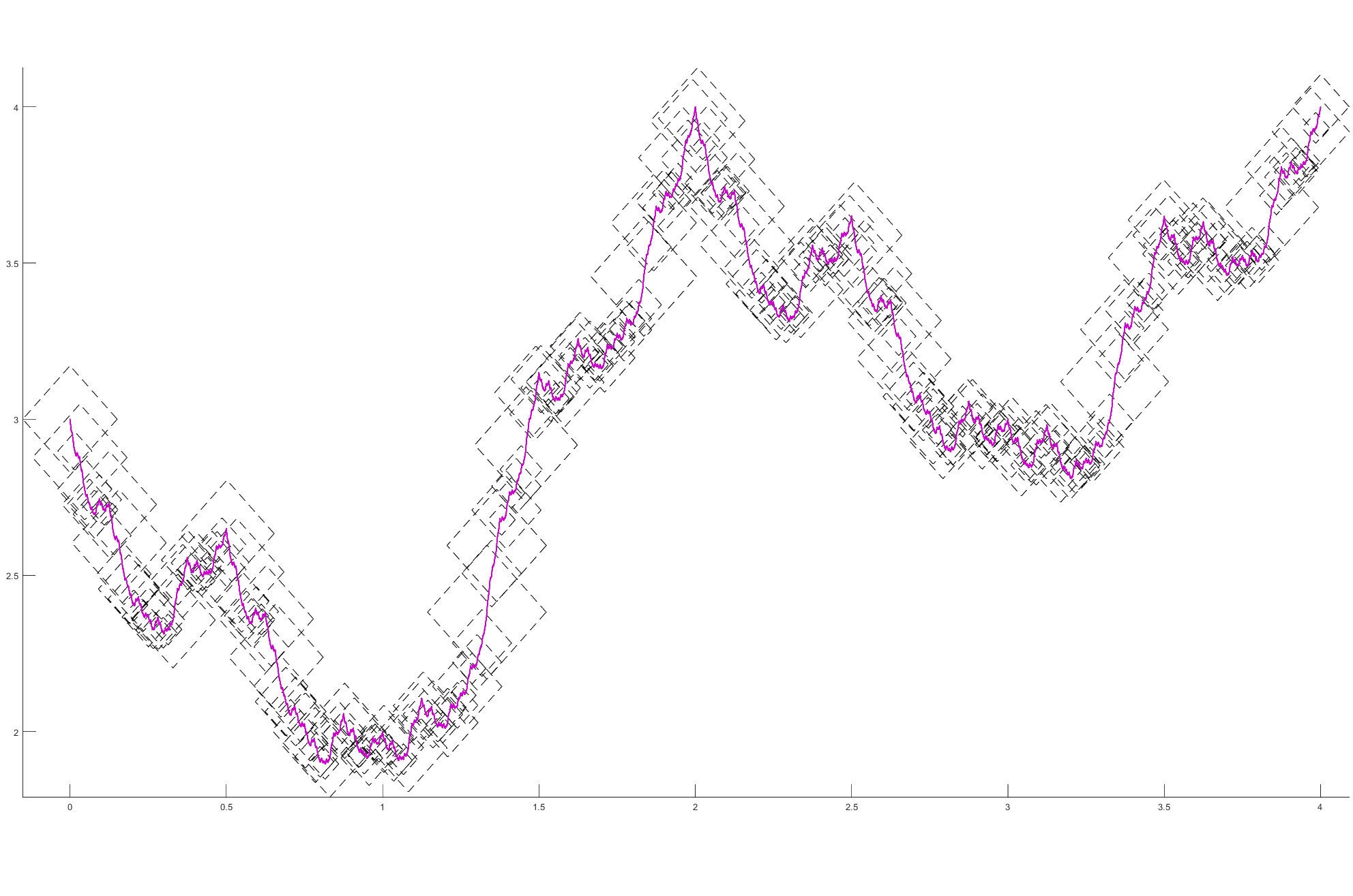
(d) $F_{14}:$ Visualization of $\mathcal{C}_{4}$

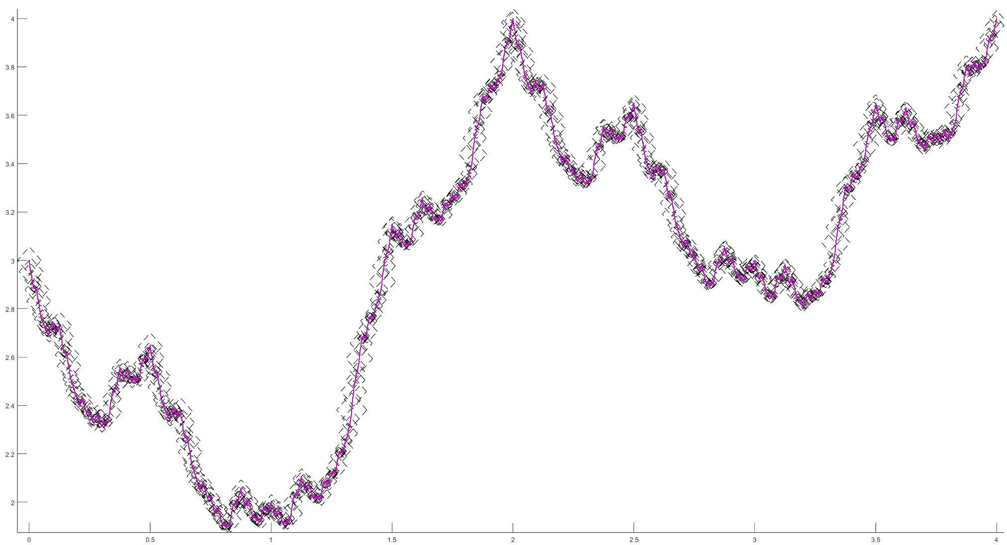
(e) $F_{15}:$ Visualization of $\mathcal{C}_{5}$

Applying Theorem 3.2 for $\mathcal{S}_{i}$, $i\in\{1,\dots,5\}$, we get

$$Imf\subseteq[A_{i},B_{i}],$$

where:

	$A_{i}$	$B_{i}$
$i=1$	-5.2218	10.8386
$i=2$	0.3859	5.5299
$i=3$	1.5986	4.4169
$i=4$	1.7899	4.1260
$i=5$	1.8744	4.0393

.

Framework 2

• the data set is

  $\{(0,4),(1,2),(2,1),(3,5),(4,7),(5,4),(6,5),(7,2),(8,4),(9,5)\}$

• $d_{k}=\frac{1}{4},$

for each $k\in\{1,\dots,9\}$.

The pictures $F_{21},F_{22},F_{23},F_{24}$ and $F_{25}$ contain the graphical representations of $\mathcal{C}_{1}$, $\mathcal{C}_{2}$, $\mathcal{C}_{3}$, $\mathcal{C}_{4}$ and respectively $\mathcal{C}_{5}$.

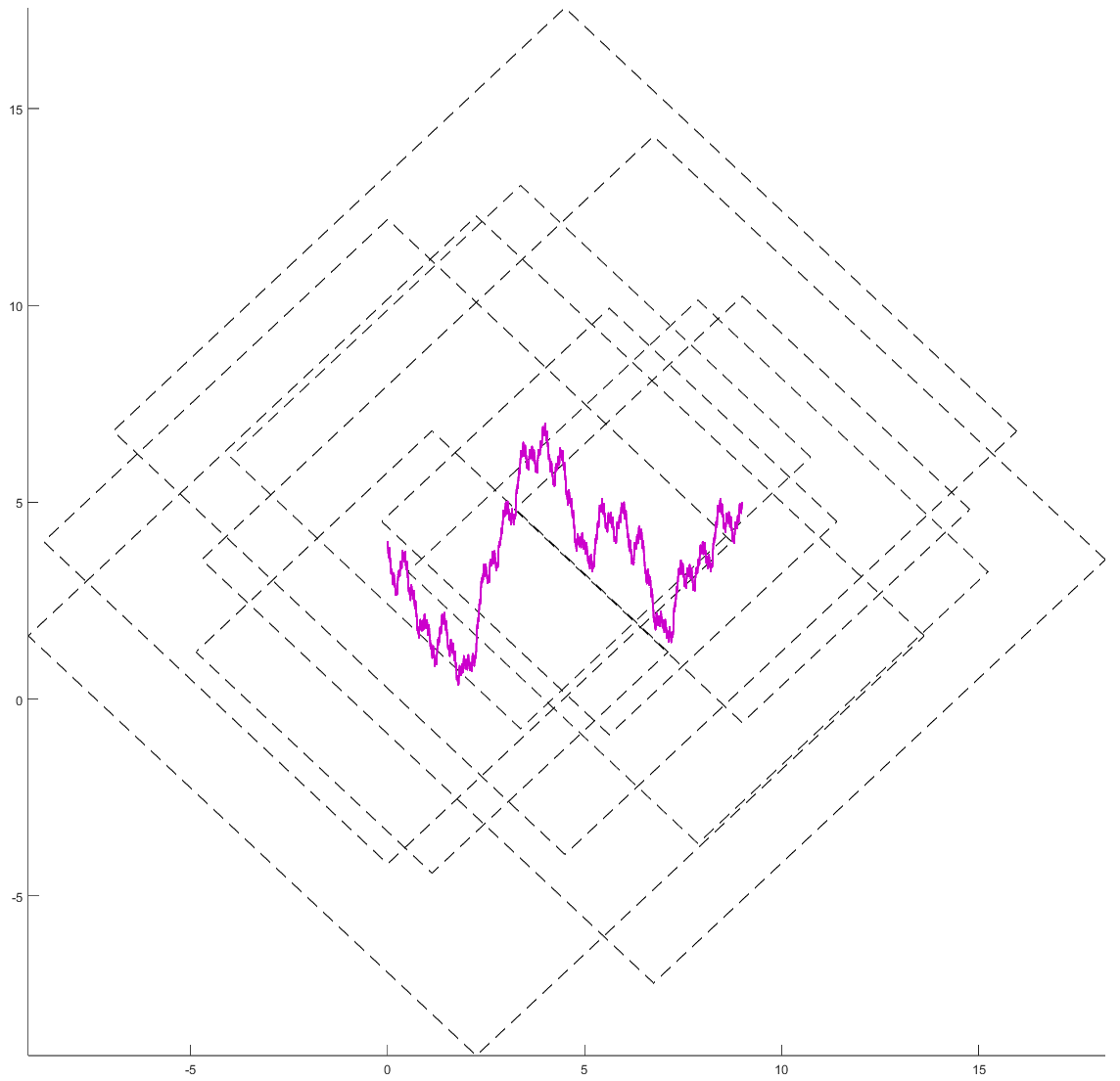
(f) $F_{21}:$ Visualization of $\mathcal{C}_{1}$

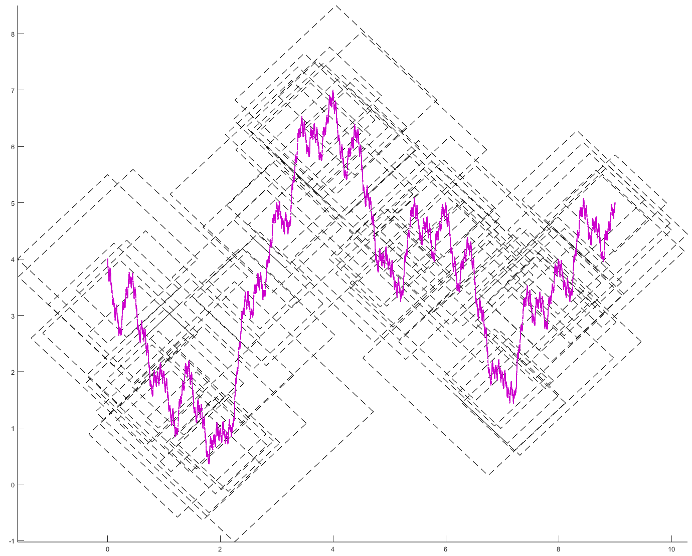
(g) $F_{22}:$ Visualization of $\mathcal{C}_{2}$

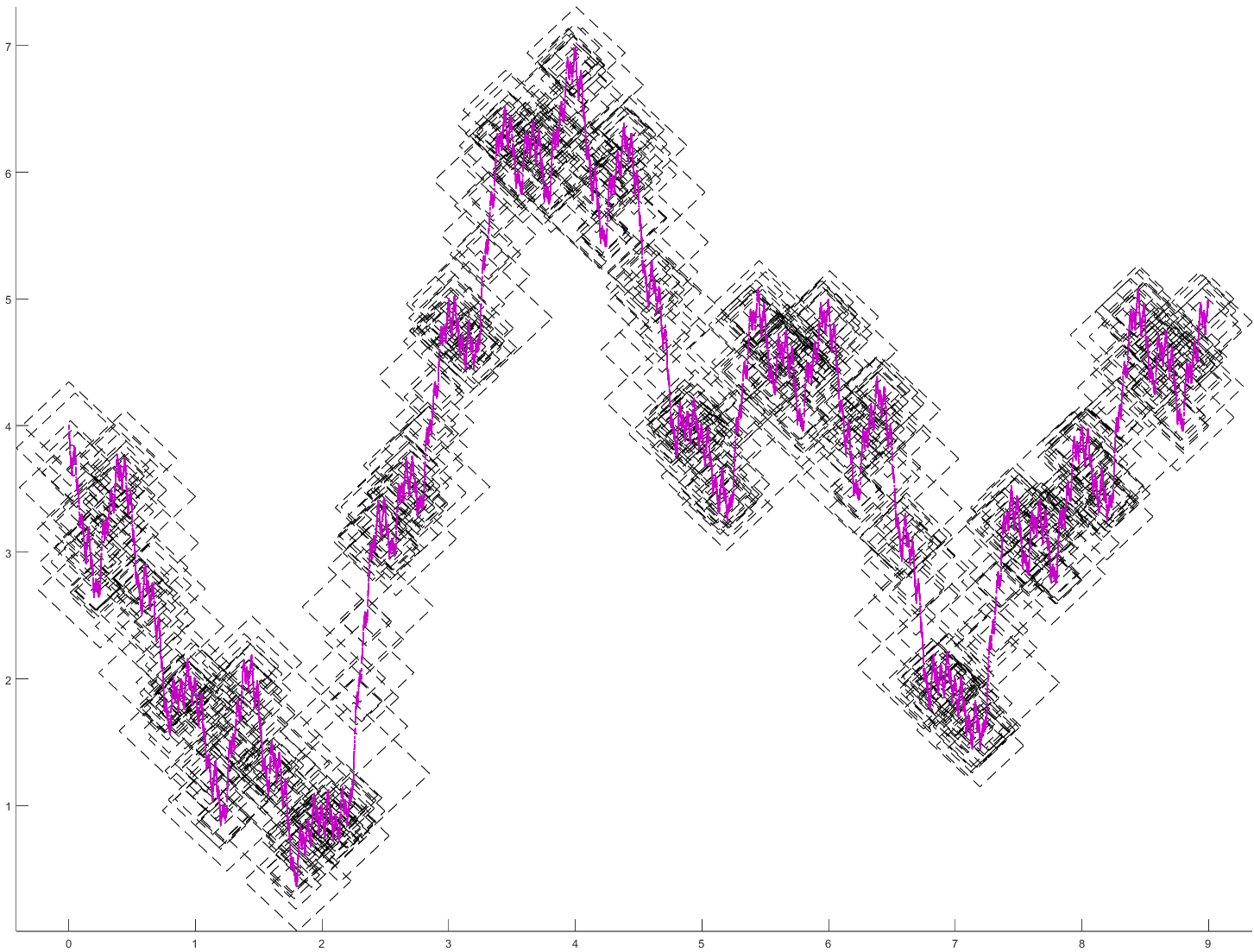
(h) $F_{23}:$ Visualization of $\mathcal{C}_{3}$

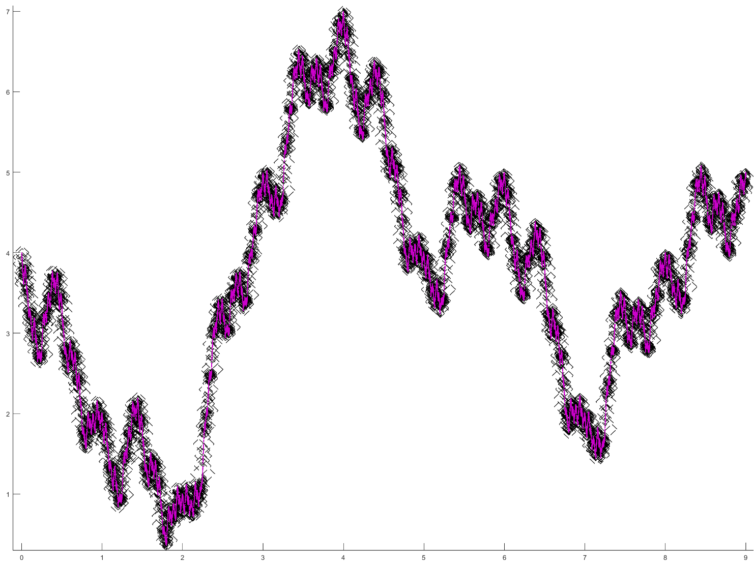
(i) $F_{24}:$ Visualization of $\mathcal{C}_{4}$

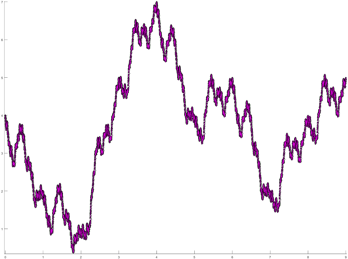
(j) $F_{25}:$ Visualization of $\mathcal{C}_{5}$

Applying Theorem 3.2 for $\mathcal{S}_{i}$, $i\in\{1,\dots,5\}$, we get

$$Imf\subseteq[A_{i},B_{i}],$$

where

	$A_{i}$	$B_{i}$
$i=1$	-9.0538	17.5588
$i=2$	-1.0068	8.4890
$i=3$	0.0069	7.3055
$i=4$	0.2998	7.0716
$i=5$	0.3393	7.0176

.

Framework 3

• the data set is

  $\{(0,0),(30,50),(60,40),(100,-10)\}$

• $d_{1}=0.5,\;d_{2}=0.5\text{ and }d_{3}=0.23.$

The pictures $F_{31},F_{32},F_{33},F_{34}$ and $F_{35}$ contain the graphical representations of $\mathcal{C}_{1}$, $\mathcal{C}_{2}$, $\mathcal{C}_{3}$, $\mathcal{C}_{4}$ and respectively $\mathcal{C}_{5}$.

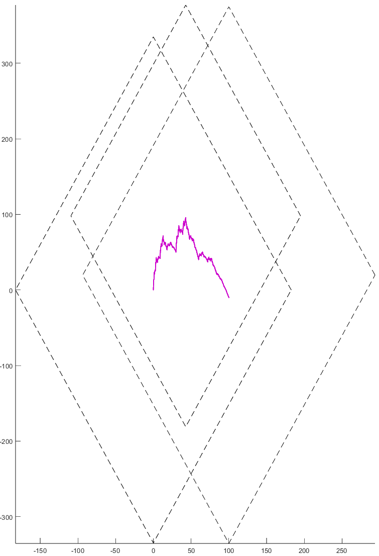
(k) $F_{31}:$ Visualization of $\mathcal{C}_{1}$

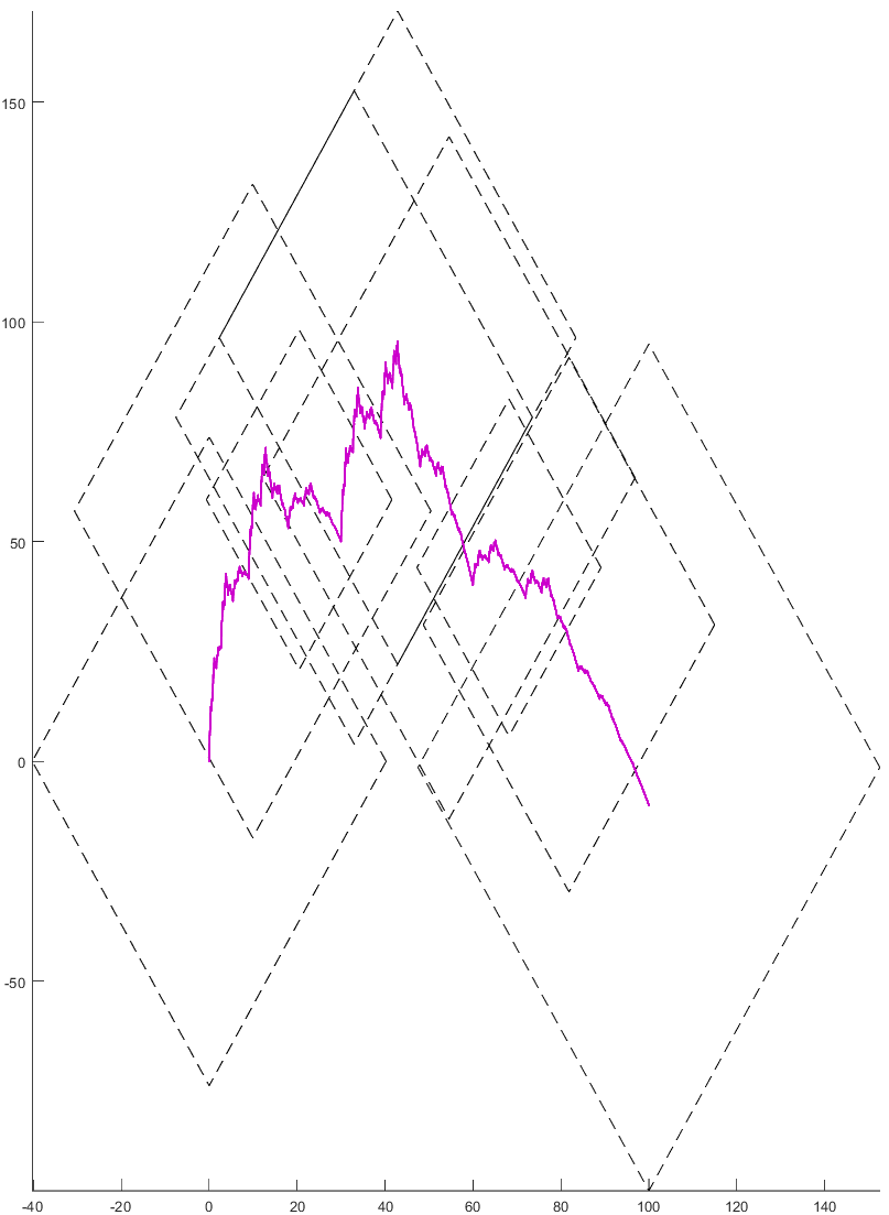
(l) $F_{32}:$ Visualization of $\mathcal{C}_{2}$

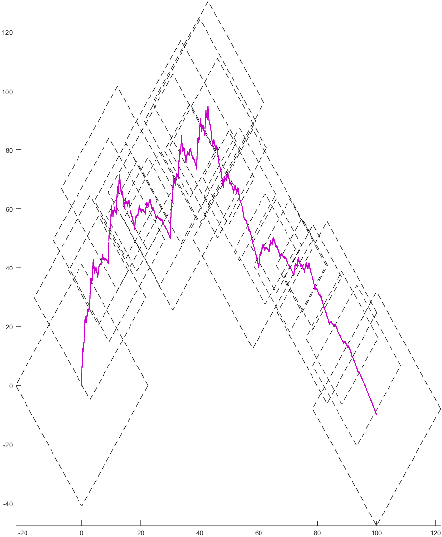
(m) $F_{33}:$ Visualization of $\mathcal{C}_{3}$

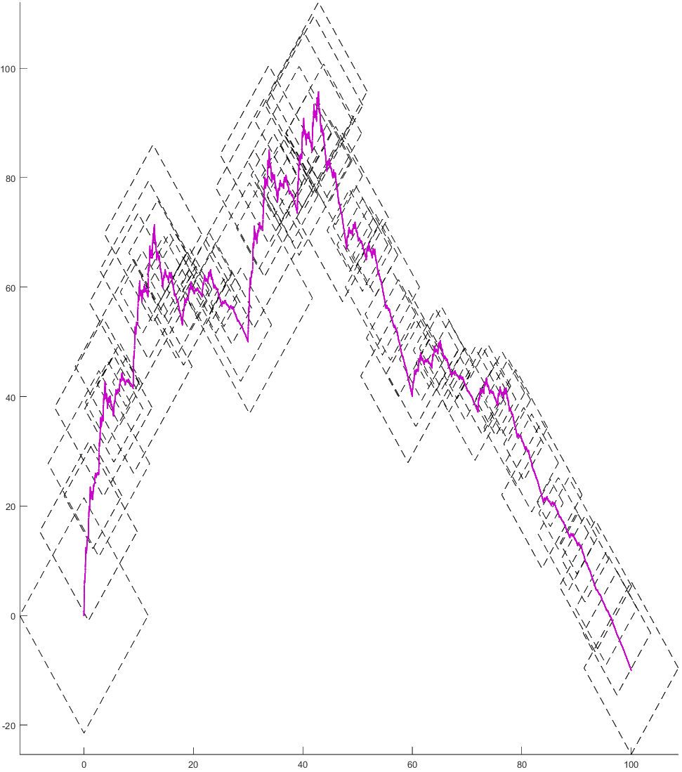
(n) $F_{34}:$ Visualization of $\mathcal{C}_{4}$

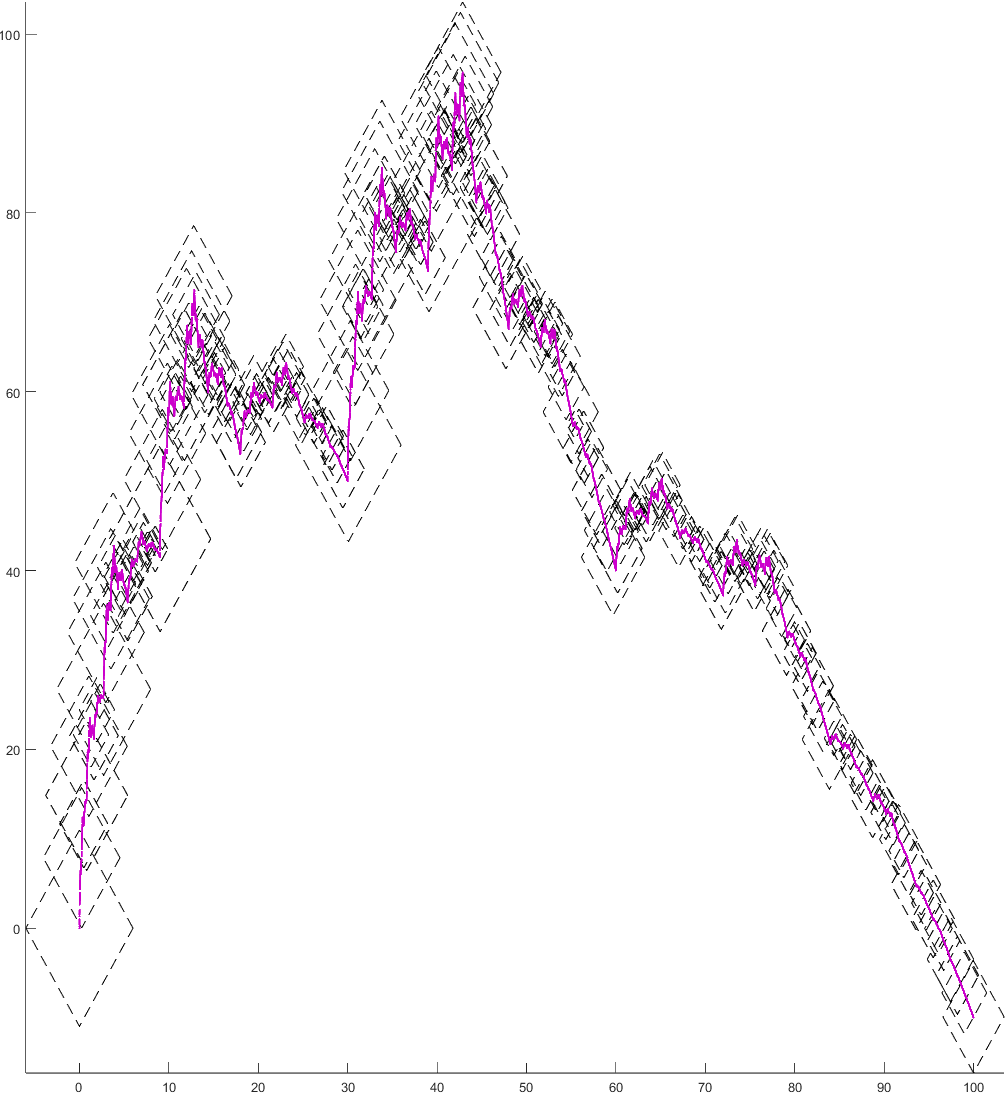
(o) $F_{35}:$ Visualization of $\mathcal{C}_{5}$

Applying Theorem 3.2 for $\mathcal{S}_{i}$, $i\in\{1,\dots,5\}$, we get

$$Imf\subseteq[A_{i},B_{i}],$$

where

	$A_{i}$	$B_{i}$
$i=1$	-335.3988	376.9781
$i=2$	-97.6725	170.6729
$i=3$	-47.7096	130.5433
$i=4$	-25.3882	112.0746
$i=5$	-16.1975	103.5866

.

Appendix

In order to find the radiuses and vertices in the previous examples we used MATLAB R2021b and the following functions:

⬇

%x and y are arrays of length n containing the data points.

%d is an array consisting of the values d_k.

function [a,b,c,e,theta] = init_coeff(x,y,d)

%This function is used to calculate the coefficients a_k,b_k,c_k,e_k and the constant theta.

l=length(x);

a=zeros(1,l-1);

b=zeros(1,l-1);

c=zeros(1,l-1);

e=zeros(1,l-1);

lip=zeros(1,l-1);

fix =zeros(2,l-1);

for i=1:l-1

a(i)=(x(i+1)-x(i))/(x(l)-x(1));

b(i)=(x(l)*x(i)-x(1)*x(i+1))/(x(l)-x(1));

c(i)=(y(i+1)-y(i))/(x(l)-x(1))-d(i)*(y(l)-y(1))/(x(l)-x(1));

e(i)=(x(l)*y(i)-x(1)*y(i+1))/(x(l)-x(1))-d(i)*(x(l)*y(1)-x(1)*y(l))/(x(l)-x(1));

end

if any(c)

theta = (1-max(a))/(2*max(abs(c)));

else

theta=1;

end

end

⬇

% m - order of composition

% p - a list consisting of all m length arrays with numbers from the set {1,2, … , n}.

% k - an array of length m with numbers from the set {1,2, … , n}.

function [a_k,b_k,c_k,d_k,e_k] = comp_k(a,b,c,d,e,m,k)

if m=1

a_k=a(k);

b_k=b(k);

c_k=c(k);

d_k=d(k);

e_k=e(k);

else

[a_t, b_t, c_t, d_t, e_t] = comp_k(a,b,c,d,e,m-1,k(2:end));

a_k = a(k(1))*a_t;

b_k = a(k(1))*b_t;

c_k = c(k(1))*a_t+d(k(1))*c_t;

d_k = d(k(1))*d_t;

e_t = c(k(1))*b_t+d(k(1))*e_t+e(k(1));

end

end

function [lipschitz_constants, fixed_points] = comp_prop(a,b,c,d,e,m,p)

%This function calculates the Lipschitz constants and fixed points of the system.

l=length(p);

lip=zeros(1,l);

fix =zeros(2,l);

for i = 1:p

[a_m,b_m,c_m,d_m,e_m]=comp_k(a,b,c,d,e,m,p(i));

lip(i)=max(d_m, a_m+theta*abs(c_m));

fix(:,i)=[b_m/(1-a_m);b_m*c_m/((1-a_m)*(1-d_m))+e_m/(1-d_m)];

end

end

⬇

% lcs - sorted array of Lipschitz constants calculated previously.

% fps - array of the fixed points calculated previously, sorted in in the order given by the Lipschitz constants.

function [r,v] = radiuses(lcs,fps)

% this function calculates the radiuses and vertices for each function in the system.

l=length(lcs);

r=zeros(1,l);

v=cell(1,l);

maxd=0;

for i=1:l-1

for j = i+1:l

n=norm(fps(:,i)-fps(:,j));

if n>maxd

maxd=n;

end

end

end

for i=1:l-1

r(i)=lcs(i)*maxd*(1+lcs(i))/(1-lcs(end)*lcs(end-1));

v{i}=[[fps(1,i)+r(i);fps(2,i)],

[fps(1,i)-r(i);fps(2,i)],

[fps(1,i);fps(2,i)+r(i)/theta],

[fps(1,i);fps(2,i)-r(i)/theta]];

end

r(l)=lcs(l)*maxd*(1+lcs(end-1))/(1-lcs(end)*lcs(end-1));

v{l}=[[fps(1,l)+r(l);fps(2,l)],

[fps(1,l)-r(l);fps(2,l)],

[fps(1,l);fps(2,l)+r(l)/theta],

[fps(1,l);fps(2,l)-r(l)/theta]];

end

end

Bogdan-Cristian Anghelina
Faculty of Mathematics and Computer Science
Transilvania University of Braov
Iuliu Maniu Street, nr. 50, 500091, Braov, Romania
E-mail: bogdan.anghelina@unitbv.ro

Radu Miculescu
Faculty of Mathematics and Computer Science
Transilvania University of Braov
Iuliu Maniu Street, nr. 50, 500091, Braov, Romania
E-mail: radu.miculescu@unitbv.ro

Mara Antonia Navascus
Departamento de Matemtica Aplicada
Universidad de Zaragoza
50018 Zaragoza Spain
E-mail: manavas@unizar.es

References

- [1] B. Anghelina, R. Miculescu, On the localization of Hutchinson–Barnsley fractals, Chaos Solitons Fractals, 173 (2023), 113674.
- [2] S. Banerjee, D. Easwaramoorthy, A. Gowrisankar, Fractal functions, dimensions and signal analysis, Springer, 2021.
- [3] M. Barnsley, Fractal functions and interpolation, Constr. Approx., 2 (1986), 303-329.
- [4] M. Barnsley, Fractals Everywhere 2nd ed., Academic Press Professional, 1993.
- [5] A.K.B. Chand, N. Vijender, P. Viswanathan, A. Tetenov, Affine zipper fractal interpolation functions, BIT, 60 (2020), 319-344.
- [6] C. Chen, S. Cheng, Y. M. Huang, The reconstruction of satellite images based on fractal interpolation, Fractals, 19 (2011), 347-354.
- [7] X. Chen, Q. Guo, L. Xi, The range of an affine fractal interpolation function, Int. J. Nonlinear Sci., 3 (2007), 181-186.
- [8] O. Crăciunescu, S. Das, J. Poulson, T. Samulski, Three-dimensional tumor perfusion reconstruction using fractal interpolation functions, IEEE Trans. Biomed. Eng., 48 (2001), 462-473.
- [9] A. Deniz, Y. Özdemir, Graph-directed fractal interpolation functions, Turkish J. Math., 41 (2017), 829-840.
- [10] V. Drakopoulos, P. Bouboulis, S. Theodoridis, Image compression using affine fractal interpolation on rectangular mattrices, Fractals, 14 (2006), 259-269.
- [11] J. Hutchinson, Fractals and self similarity, Indiana Univ. Math. J., 30 (1981), 713-747.
- [12] K. Gdawiec, Fractal interpolation in modeling of 2D contours, Int. J. Pure Appl. Math., 50 (2009), 421-430.
- [13] M. Leon-Ogazon, E. Romero-Flores, T. Morales-Acoltzi, A. Machorro, M. Salazar-Medina, Fractal interpolation in the financial analysis of a company, Int. J. Bus. Adm., 8 (2017), 80-86.
- [14] J. Lu, J. Wu, H. Yao, J. Qian, Z. Wang, J. Wang, Predicting river dissolved oxygen in complex watershed by using sectioned variable dimension fractal method and fractal interpolation, Environ. Earth Sci., 66 (2012), 2129-2135.
- [15] D. Luor, Fractal interpolation functions with partial self similarity, J. Math. Anal. Appl., 464 (2018), 911-923.
- [16] P. Manousopoulos, V. Drakopoulos, E. Polyzos, Financial time series modelling using fractal interpolation functions, AppliedMath, 3 (2023), 510-524.
- [17] P. Manousopoulos, V. Drakopoulos, T. Theoharis, Parameter identification of 1D fractal interpolation functions using bounding volumes, J. Comput. Appl. Math, 233 (2009), 1063-1082.
- [18] P. Massopust, Vector-valued fractal interpolation functions and their box dimension, Aequationes Math., 42 (1991), 1-22.
- [19] P. Massopust, Interpolation and approximation with splines and fractals. Oxford University Press, Oxford, 2010.
- [20] P. Massopust, Local fractal interpolation on unbounded domains, Proc. Edin. Math. Soc, 61 (2018), 151-167.
- [21] R. Miculescu, A. Mihail, C. Păcurar, A fractal interpolation scheme for a possible sizeable set of data, J. Fractal Geom., 9 (2022), 337-355.
- [22] M. Navascués, A fractal approximation to periodicity, Fractals, 14 (2006), 315-325.
- [23] M. Navascués, Reconstruction of sampled signals with fractal functions, Acta Appl. Math., 110 (2010), 1199-1210.
- [24] M. Navascués, A. K. B. Chand, V. P. Veedu, M. Sebastián, Fractal interpolation functions: a short survey, Appl. Math., 5 (2014), 1834-1841.
- [25] M.A. Navascués, M.V. Sebastián. Error bounds for affine fractal interpolation. Math. Ineq. Appl., 9 (2006), 273-288.
- [26] M.A. Navascués, M.V. Sebastián. Numerical integration of affine fractal functions, J. Comp. Appl. Math., 252 (2013), 169-176.
- [27] M. Navascués, M. Sebastián, Some historical precedents of the fractal functions, Fractals, wavelets, and their applications, 271-282, Springer Proc. Math. Stat., 92, Springer, Cham, 2014.
- [28] S. Ri, A new idea to construct the fractal interpolation function, Indag. Math., 29 (2018), 962-971.
- [29] D. Riccio, N. Brancati, G. Sannino, L. Verde, M. Frucia, CNN-based classification of phonocardiograms using fractal techniques, Biomedical Signal Processing and Control, 86 (2023), 105186.
- [30] H. Stanley, S. Buldyrev, A. Goldberger, J. Hausdorff, S. Havlin, J. Mietus, C. Penk, F. Sciortino, M. Simons, Fractal landscape in biological systems: long-range correlations in DNA and interbeat heart intervals, Physica A, 191 (1992), 1-12.
- [31] S. Vasil’ev, Fractal interpolation methods of Barnsley, Russian Math., 46 (2002), 1-12.
- [32] P. Viswanathan, A.K.B. Chand, M. Navascués, Fractal perturbation preserving fundamental shapes: bounds on the scale factors, J. Math. Anal. Appl., 419 (2014), 804-817.
- [33] H. Wang, J. Yu, Fractal interpolation functions with variable parameters and their analytical properties, J. Approx. Theory, 175 (2013), 1-18.
- [34] H. Xie, H. Sun, Y. Ju, Z. Feng, Study on generation of rock fracture surfaces by using fractal interpolation, Int. J. Solid Struct., 38 (2001), 5765-5787.
- [35] C. Xiu, T. Wang, M. Tian, Y. Li, Y. Cheng, Short term prediction method of wind speed based on fractal interpolation, Chaos Solitons Fractals, 68 (2014), 89-97.
- [36] M. Zhai, J. Fernádez-Martínez, A new fractal interpolation algorithm and its applications to self-affine signal reconstruction, Fractals, 19 (2011), 355-365.