First Sagittarius A^∗ Event Horizon Telescope Results VI: Testing the Black Hole Metric

Abstract

Astrophysical black holes are expected to be described by the Kerr metric. This is the only stationary, vacuum, axisymmetric metric, without electromagnetic charge, that satisfies Einstein’s equations and does not have pathologies outside of the event horizon. We present new constraints on potential deviations from the Kerr prediction based on 2017 EHT observations of Sagittarius A^∗ (Sgr A^∗). We calibrate the relationship between the geometrically defined black hole shadow and the observed size of the ring-like images using a library that includes both Kerr and non-Kerr simulations. We use the exquisite prior constraints on the mass-to-distance ratio for Sgr A^∗ to show that the observed image size is within $\sim 10\%$ of the Kerr predictions. We use these bounds to constrain metrics that are parametrically different from Kerr as well as the charges of several known spacetimes. To consider alternatives to the presence of an event horizon we explore the possibility that Sgr A^∗ is a compact object with a surface that either absorbs and thermally re-emits incident radiation or partially reflects it. Using the observed image size and the broadband spectrum of Sgr A^∗, we conclude that a thermal surface can be ruled out and a fully reflective one is unlikely. We compare our results to the broader landscape of gravitational tests. Together with the bounds found for stellar mass black holes and the M87 black hole, our observations provide further support that the external spacetimes of all black holes are described by the Kerr metric, independent of their mass.

1 Introduction

Horizon-scale images of supermassive black holes provide a conceptually new avenue for testing the theory of General Relativity. These images are formed by photons that originate in the deep gravitational fields of black holes, and, therefore, carry imprints of the spacetime properties in the strong-field regime (Jaroszynski & Kurpiewski, 1997; Falcke et al., 2000). In this series of papers, we report the first horizon-scale images of Sgr A^∗, the black hole at the center of our Galaxy, obtained with the Event Horizon Telescope (EHT), a global interferometric array observing at 1.3 mm wavelength (Event Horizon Telescope Collaboration et al. 2022a, b, hereafter papers II and III). This paper in the series explores new constraints on the potential deviations from General Relativity imposed by these images.

General Relativity has been tested in numerous settings with different observational tools and with different astrophysical systems (see the review by Will 2014 and references therein). Traditionally, tests have been carried out in the solar system, with the periastron precession of Mercury (Verma et al., 2014), the deflection of light observed during solar eclipses (Lambert & Le Poncin-Lafitte, 2011), and the detection of Shapiro delays in photons grazing the solar surface (Bertotti et al., 2003). Radio observations of pulsars in binary systems expanded these tests, probing the radiative aspects of the theory and the strong-field coupling of the matter to the gravitational field (see Stairs 2003 for a review and Wex & Kramer 2020; Kramer et al. 2021 for some recent examples). Cosmological observations of the accelerated expansion of the universe probed gravity at the largest scales in the cosmos and gave evidence for the presence of dark matter and dark energy (see Ferreira 2019 for a review).

As is clear from this overview, each test probes a different aspect of the theory of General Relativity. First, different astrophysical objects possess widely different mass and length scales and hence map to a very broad range of gravitational potentials and curvatures (Baker et al., 2015). Second, some tests probe the stationary spacetimes of objects while others probe the dynamic and radiative aspects of the theory. Third, some settings involve vacuum spacetimes while others are affected by the coupling of matter and radiation to gravity (see, e.g., Damour & Esposito-Farese 1993). Because modifications to the theory of gravity can be introduced independently in each of these aspects, without necessarily affecting the others, each of these tests brings a unique ability to constrain such modifications.

Although general relativistic predictions have shown a high degree of consistency with the aforementioned tests, there remain unresolved questions at the fundamental level; e.g., whether curvature singularities are generally covered by event horizons (cosmic censorship conjecture) or can be naked. These become most urgent for black holes as those objects have the strongest gravitational fields in the universe and possess a curvature singularity in their center. The combination with quantum theory could tame curvature singularities but at the same time predicts inherent randomness for quantum particles at the event horizon leading to the black hole information loss paradox (see, e.g., Harlow 2016 for a review). All the concerns involve the presence of event horizons and are, therefore, accessible only to tests with black holes. Until recently, however, precision tests of gravity with black holes have not been possible. This situation has changed dramatically in the recent years with the detection of gravitational waves from coalescing stellar mass black holes with LIGO/Virgo (Abbott et al., 2016, 2021), the detection of relativistic effects in the orbits of stars around Sgr A^∗ (Gravity Collaboration et al., 2018a; Do et al., 2019; Gravity Collaboration et al., 2020a), and the imaging observations of the black hole in the center of the M87 galaxy (Event Horizon Telescope Collaboration et al., 2019c; Psaltis et al., 2020a; Kocherlakota et al., 2021).

Tests of gravity with black holes benefit from a remarkable General Relativistic prediction encapsulated in the so-called no-hair theorem: the only vacuum spacetime that is stationary, axisymmetric, asymptotically flat, contains a horizon and is free of pathologies is the one described by the Kerr metric (Kerr, 1963; Israel, 1967, 1968; Carter, 1968, 1971; Hawking, 1972; Price, 1972a, b; Robinson, 1975). Testing this prediction involves using spacetimes that introduce deviations from this metric and applying observational constraints to place bounds on the magnitudes of the deviations. In order for these spacetimes to evade the no-hair theorem while remaining free of pathologies, they cannot be solutions to the vacuum General Relativistic field equations but instead involve additional fields or parametric deviations that are agnostic to the underlying theory of gravity. In either case, measuring conclusively a deviation from the Kerr metric, while demonstrating that the compact object has a horizon, will constitute a demonstration of a violation of the no-hair theorem and, therefore, of the General Relativistic field equations.

Horizon-scale images of Sgr A^∗ offer a distinct set of advantages in testing General Relativistic predictions with black holes (Psaltis & Johannsen, 2011; Psaltis et al., 2016; Goddi et al., 2017; Cunha & Herdeiro, 2018; Psaltis, 2019). At $4\times 10^{6}M_{\odot}$, this black hole has a mass that bridges those of the stellar-mass black holes observed with LIGO/Virgo ($\sim 10^{1}-10^{2}M_{\odot}$) and that of the M87 black hole ($\sim 6.5\times 10^{9}M_{\odot}$), and, therefore, probes a curvature scale that is different from those of other tests. Perhaps more importantly, it enables an approach that is different from other tests in its methodology. Because of the detection of relativistic effects in the stellar orbits around this black hole, its mass and distance are accurately known resulting in precise predictions of its space time properties (Do et al., 2019; GRAVITY Collaboration et al., 2022). As a result, contrary to other tests, where the mass of the black hole is measured from the same data simultaneously with the other spacetime properties (or possess significant astrophysical uncertainties as in M87), tests with Sgr A^∗ rely on mass priors with completely orthogonal systematics and potential biases. In addition, the very small uncertainties in the prior mass measurement lead to a parameter-free prediction on the gravitational effects in the images, which can be tested precisely with the EHT observations.

The most prominent gravitational effect on black hole images is the black hole shadow (Falcke et al., 2000). The boundary of the shadow on the image plane of a distant observer is marked by the impact parameters of photons, which, when traced back towards the black hole, become tangent to the spherical photon orbits close to the horizon (Bardeen, 1973; Luminet, 1979). Although we define the shadow as a purely geometric feature that does not depend on astrophysical effects, we relate this feature to the brightness depression in observed images. Photons with impact parameters smaller than this critical value have paths that cross the horizon and, hence, have small optical paths through this spacetime. These reduced optical paths lead to much smaller radiation intensities compared to photons at larger impact parameters and, therefore, to the brightness depression (Jaroszynski & Kurpiewski, 1997; Johannsen & Psaltis, 2010; Narayan et al., 2019; Özel et al., 2021; Bronzwaer & Falcke, 2021; Kocherlakota & Rezzolla, 2022).

In the Kerr metric, because of a cancellation between the effects of frame dragging and the quadrupole moment of the spacetime, the shape and size of the shadow boundary have a very weak dependence on black hole spin and the observer’s inclination (i.e., the radius ranges from $\sim 4.8GMc^{-2}$ to $\sim 5.2GMc^{-2}$, see Johannsen & Psaltis 2010 for a detailed study of the dependence on spin). Instead, they are determined predominantly by the mass-to-distance ratio of the black hole, which are known precisely for Sgr A^∗, making the shadow a direct probe of the metric properties (see e.g., Psaltis et al. 2015). For the black hole shadow to become observable, two conditions need to be satisfied. First, a sufficiently bright source of photons needs to be present close to the horizon such that these photons experience strong gravitational lensing. Second, this source needs to be optically thin (i.e., transparent) at the observing wavelength such that the shadow is not enshrouded by the material generating this radiation. Both of these conditions are satisfied at 1.3 mm in the radiatively inefficient accretion flow around Sgr A^∗  (Özel et al. 2000; see also Event Horizon Telescope Collaboration et al. 2022d, hereafter Paper V).

For such a configuration, the predicted image of the black hole is a bright ring of emission surrounding the shadow. The imaging observations with the EHT capture this ring and allow us to measure its properties, such as its diameter and fractional width. Earlier work has shown that, when this ring of emission is observed, the ring diameter can be used, with proper calibration, as a proxy for the shadow diameter itself (Event Horizon Telescope Collaboration et al., 2019b, c; Narayan et al., 2019; Özel et al., 2021; Younsi et al., 2021; Kocherlakota & Rezzolla, 2022). This is the approach that we follow in this paper to compare the predictions of General Relativity for the size of the black hole shadow to the observed measurement of the ring in the images of Sgr A^∗.

The presence of a brightness depression also allows us to explore different possibilities for the nature of the compact object itself. In particular, if Sgr A^∗ contained a reflecting surface at 1.3 mm instead of a horizon or a naked singularity, we would have observed a less pronounced brightness depression. Alternatively, if it contained a surface that was fully absorptive and reemitting thermally the accreting energy, it would still create a depression in the EHT image but would generate bright emission at wavelengths shorter than 1.3 mm. We use the EHT images in conjunction with the broadband spectrum of Sgr A^∗ to place strong constraints on such alternatives.

In Section 2, we summarize the prior information on the mass-to-distance ratio and the spectrum of Sgr A^∗. In Section 3, we quantify the measurements of the image diameter as well as the relationship between image and shadow diameters using extensive simulations and synthetic data. We combine these to place bounds on potential deviations between the predicted and inferred shadow size for Sgr A^∗. In Section 4, we constrain alternatives to the black hole nature of the compact object that involve reflecting or absorbing surfaces. In Section 5, we impose constraints on the potential metric deviations from Kerr as well as address the possibility that Sgr A^∗ contains a naked singularity. In Section 6, we leverage our gravity tests with those that involve other compact objects and solar system bodies in order to draw general conclusions about the theory of gravity. We summarize our findings in Section 7.

2 Priors

2.1 Priors on $\theta_{g}$

The mass and distance of Sgr A^∗ have been extensively studied by analyzing the dynamics of the central stellar cluster in the innermost 10 arcsec of the Galactic Center (Genzel et al., 1997; Ghez et al., 1998; Eckart et al., 1999; Genzel et al., 2000; Ghez et al., 2000; Eckart et al., 2002; Gezari et al., 2002; Genzel et al., 2003b; Schödel et al., 2007; Martins et al., 2008; Genzel et al., 2010; Morris et al., 2012; Do et al., 2013; Jia et al., 2019). Near-infrared observation with 8-m to 10-m class telescopes supported by adaptive optics (AO) revealed the orbits of individual stars in the innermost arcsec (the so-called S-stars), in particular the star S0-2 For this star, the combined fit for orbital elements and black hole parameters (mass, distance, projected position in the sky, proper motions, and radial velocity) has provided the most precise estimates for Sgr A^∗’s mass and distance so far (Schödel et al. 2003; Ghez et al. 2005a; Eisenhauer et al. 2005; Ghez et al. 2008; Gillessen et al. 2009b, a; Meyer et al. 2012; Boehle et al. 2016; Gillessen et al. 2017; Chu et al. 2018; O’Neil et al. 2019; Hees et al. 2019; Gravity Collaboration et al. 2021a).

S0-2 is a star with an apparent $2.2$ $\mu$m (NIR K-band) magnitude of $m_{K}=14$, an orbital period of $P\approx 16$ years, a semi-major axis of $a=125$ mas (or $\sim 10^{3}$ AU at an 8 kpc distance), and, thus, is the brightest star with a comparatively close orbit and short period at the Galactic Center. The study of S0-2’s orbit has predominantly been conducted with two sets of instruments, the two 10-m telescopes of the Keck Observatory, and the Very Large Telescope (VLT) of the European Southern Observatory (ESO), using its individual telescopes as well as GRAVITY, an interferometer combining all four 8.2-m telescopes of the VLT (VLTI). The orbit of S0-2 provides some of the best evidence for the existence of a black hole. S0-2 has concluded an entire revolution between 2002 and 2018 covered by observations and has allowed the Keck and VLTI teams to test relativistic effects like the gravitational redshift or the Schwarzschild precession (Gravity Collaboration et al. 2020a; Do et al. 2019; Gravity Collaboration et al. 2018a, 2019; Amorim et al. 2019) and to constrain alternative theories of gravity (Hees et al. 2017; De Martino et al. 2021; Della Monica et al. 2021) and variations of the fine structure constant (Hees et al. 2020).

Figure 1: Posteriors on $\theta_{\rm g}=GM/Dc^{2}$ as derived from the dynamical analyses of the orbit of the Galactic Center star S0-2 by the Keck and the VLTI teams, respectively.

In order to measure S0-2’s projected position in the sky, an astrometric reference frame has to be established. Menten et al. (1997) proposed the idea to use a group of SiO maser stars at the Galactic Center — visible both in the radio as well as in the NIR — with positions and proper motions determined by interferometric astrometry at radio wavelengths. These masers allow it to establish a reference frame in the NIR. For both imaging instruments (KeckII/NIRC2, VLT/NACO) the field of view (10 arcsec and 14 arcsec, respectively) is not large enough to capture the S-stars and the seven masers in the same pointing. Instead, a dither pattern of pointings overlapping with one another is observed. Astrometric measurements in the central field are then executed via secondary astrometric standards, either in the form of matching coordinate lists or by generating mosaic images. In this process, systematic astrometric errors occur due to the geometric distortions of the camera optics and field dependence of the point spread function (PSF) caused by anisoplanatism of the AO-correction and higher order aberrations of the optics (Yelda et al. 2010; Plewa et al. 2015; Sakai et al. 2019).

The VLTI team included interferometric data in their analysis starting in 2016. VLTI/GRAVITY provided high precision distance measurements to Sgr A^∗ during the S0-2’s closest approach with $\sim$1 mas resolution and $\sim 40\,\mu$as astrometric precision.

This subset of the interferometric data is not affected by the systematic uncertainties of the reference frame because the projected position of S2 is directly referenced to the projected (center of light) position of Sgr A*. However, also VLTI/GRAVITY data have systematic uncertainties, mainly due to aberrations of the optical trains of the individual telescopes (Gravity Collaboration et al. 2021b).

Information on the third dimension of the stellar orbits is obtained in the form of radial velocities, which in the case of S0-2 can be determined by observing the 2.167 $\mu$m HI (Br$\gamma$) and the 2.11 $\mu$m HeI lines with integral field spectrographs like VLT/SINFONI or Keck/OSIRIS.

In their latest publication on the measurement of the gravitational redshift (Do et al. 2019, Table 1) the Keck team found for the distance a value of $(R_{0}=7959\pm 59\pm 32)$ pc (for the fit that leaves the redshift parameter free). They also published a posterior version with the assumption that General Relativity is true (redshift parameter set to unity), $R_{0}=(7935\pm 50)$ pc, which is practically equivalent within the uncertainties. Their estimates for the black hole mass are $M=(3.975\pm 0.058\pm 0.026)\times 10^{6}M_{\odot}$ and $M=(3.951\pm 0.047)\times 10^{6}M_{\odot}$, respectively.

In the publication on the detection of the Schwarzschild precession (Gravity Collaboration et al. 2020a), the VLTI team found $R_{0}=(8246.7\pm 9.3)$ pc and $M=(4.261\pm 0.012)\times 10^{6}M_{\odot}$. Their latest paper on the mass distribution in the Galactic Center (GRAVITY Collaboration et al. 2022) changes these values slightly. Their table B.1 is an overview of recently published VLTI values for the black hole mass and distance; they also give an estimate of their systematics due to aberrations in GRAVITY’s optics: $R_{0}=(8277\pm 9\pm 33)$ pc (Gravity Collaboration et al. 2021b). For the mass they find: $M=(4.297\pm 0.012\pm 0.040)\times 10^{6}M_{\odot}$. Additionally, the team provided a file with the posterior chains of their Bayesian analysis (Gillessen, priv. communication), assuming General Relativity to be true, which has median values of $R_{0}=(8278\pm 10)$ pc and $M=(4.298\pm 0.013)\times 10^{6}M_{\odot}$.

It is interesting to point out that a third, independent estimate for the distance to Sgr A^∗ has been provided by the Bessel project, a study of the Milky Way structure with VLBI astrometry: $R_{0}=(8.15\pm 0.15)$ kpc (Reid et al. 2009, 2014, 2019). This value for the distance is in marginally better agreement with the VLTI results.

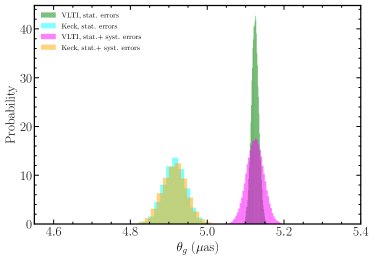
Here, the two values considered for the distance are $R_{0}=(7935\pm 50\pm 32)$ pc and $R_{0}=(8277\pm 9\pm 33)$ pc. Mass and distance set a characteristic scale of the orbit in its projection on the sky and are highly correlated. The values for $\theta_{g}\equiv GM/Dc^{2}$ as derived from the posterior distributions are: $\theta_{g}=(5.125\pm 0.009\pm 0.020)\,\mu$as (VLTI) and $\theta_{g}=(4.92\pm 0.03\pm 0.01)\,\mu$as (Keck). For the VLTI value, the systematics were derived by error propagation according to $M\propto R_{0}^{2}$ (GRAVITY Collaboration et al. 2022). For the Keck value, a dedicated jackknife analysis was conducted to quantify the systematics stemming from the reference system (Do, priv. communication). We show the posteriors in Figure 1. The discrepancy between the values of the two studies is about 4%.

Figure 2: Sgr A^∗ radio to X-ray Spectral Energy Distribution (SED). Blue points show re-binned observed flux densities (Falcke et al. 1998; An et al. 2005; Bower et al. 2015; Liu et al. 2016; Bower et al. 2019), the faint colored points show upper limits for the median flux density from the papers listed on the right. Solid gray lines from 4.5 to 2.2 $\mu$m show model SEDs for the 5th, 50th, and 95th percentile and demonstrate the predicted slope change as a function of flux density. The green points at 2.2 $\mu$m represent the most recent analysis of the 5th, 50th, and 95th percentile of NIR flux density distribution based on VLTI/GRAVITY data. The orange-shaded envelope represents an estimate of the range of flux densities in 90% of the observed time.

2.2 Priors on the spectral energy distribution of Sgr A^∗

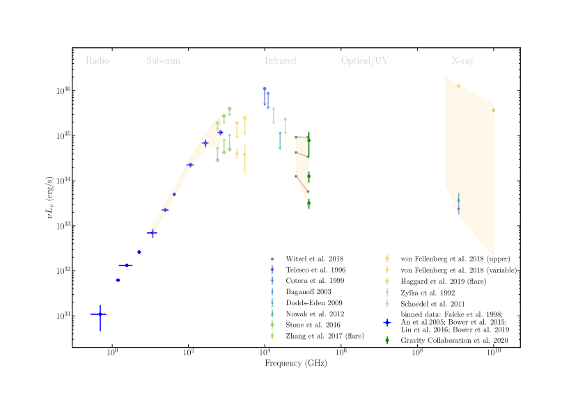
The spectral energy distribution (SED) of Sgr A^∗ is shown in Figure 2. It has been compiled from the large body of literature, starting as early as 1992. Points show SED values taken from Zylka et al. (1992); Telesco et al. (1996); Falcke et al. (1998); Cotera et al. (1999); An et al. (2005); Dodds-Eden et al. (2009); Schödel et al. (2011); Dodds-Eden et al. (2011); Nowak et al. (2012); Bower et al. (2015); Liu et al. (2016); Stone et al. (2016); Zhang et al. (2017); von Fellenberg et al. (2018); Witzel et al. (2018); Bower et al. (2019); Haggard et al. (2019); Gravity Collaboration et al. (2020b). We present the radio part of the SED (Falcke et al. 1998; An et al. 2005; Bower et al. 2015; Liu et al. 2016; Bower et al. 2019) in a binned version (for a more detailed version showing all historic literature values in the radio to sub-millimeter regime, including some epochs of heightened variability, see Paper II). The steepening of the SED slope at cm wavelengths (Falcke et al. 1998), is clearly visible between 10-20 GHz and the sub-millimeter. From THz-frequencies to the mid IR Sgr A^∗ has not be detected, and we have included lower and upper limits.

The SED shows variability in all observable parts. Especially in the NIR and X-ray regime Sgr A^∗ is strongly variable with regular flux density changes of factors of tens and hundreds, respectively, within $10-20$ min (e.g., Baganoff et al. 2001; Genzel et al. 2003a; Eckart et al. 2004a; Ghez et al. 2005b; Do et al. 2009; Dodds-Eden et al. 2011; Witzel et al. 2012; Neilsen et al. 2013, 2015; Ponti et al. 2017; Fazio et al. 2018). However, at radio frequencies and in the mm/sub-millimeter regime the variability is comparatively minor with typical excursions of about 50% or less of the mean flux density. (Falcke 1999; Herrnstein et al. 2004; Marrone et al. 2008; Dexter et al. 2014; Brinkerink et al. 2015; Subroweit et al. 2017; Fazio et al. 2018; Murchikova & Witzel 2021; Goddi et al. 2021).

Here we are focusing on the NIR properties of Sgr A^∗, in particular on limits for a steady component that is not varying on timescales of minutes and hours. Figure 2 shows the percentiles of the observed flux density distributions at 2.2 $\mu$m (VLT/NACO and KECK/NIRC2) and 4.5 $\mu$m (SPITZER/IRAC) as well as the corresponding spectral indices that change with flux density (Witzel et al., 2018). Additionally, we present the same percentiles for the flux density distribution measured with VLTI/GRAVITY at 2.2 $\mu$m (Gravity Collaboration et al., 2020b). While the VLT and KECK data are confusion limited and noise dominated at the low end of flux density distribution resulting in non-detections of the source against the background, Gravity Collaboration et al. (2020b) report a clear detection of Sgr A^∗ at all times. Because this detected source is variable at all times, their 5th percentile of the variable flux density distribution represents a conservative upper limit for any steady source component that may lie underneath.

3 EHT Observations and Error budget

The EHT observations of Sgr A^∗ show a bright ring of emission surrounding a brightness depression that we have identified with the black hole shadow (Event Horizon Telescope Collaboration et al., 2022b). In principle, the diameter of this ring, $\hat{d}_{m}$, can be used to measure the properties of the black hole metric and to assess its compatibility with the Kerr solution in General Relativity for a black hole of given angular size $\theta_{g}$. In practice, this comparison first requires establishing a quantitative relation (i.e., a calibration factor) between the diameter of a bright ring feature and that of the corresponding shadow. We can then use this relationship, in combination with the measured ring diameter, to infer any potential deviations from the General Relativistic predictions.

To accomplish this, we write

$$\hat{d}_{m} = \frac{\hat{d}_{m}}{d_{\rm sh}}d_{\rm sh}=\alpha_{\rm c}\;d_{\rm sh}=\alpha_{\rm c}\;(1+\delta)\;d_{\rm sh,Sch}$$ (1)

$$= \alpha_{\rm c}\;(1+\delta)\;6\sqrt{3}\;\theta_{g}\;.$$

In this expression, $\hat{d}_{m}$ is the ring diameter measured from imaging and model-fitting to the Sgr A^∗ data, where the hat signifies the fact that this is a measured quantity that may differ from the true value because of measurement biases. The quantity $\alpha_{\rm c}\equiv\hat{d}_{m}/d_{\rm sh}$ is the calibration factor, defined as the ratio of the measured diameter of the image to that of the shadow, which addresses the extent to which the ring diameter can be used as a proxy for the shadow diameter. The shadow diameter depends on the metric and its properties, such as the black-hole spin and potential charges, as well as on the observer inclination.

The calibration factor $\alpha_{\rm c}$ is determined primarily by the physics of image formation near the horizon and quantifies the degree to which the image diameter tracks that of the shadow, for any underlying metric and for different realistic models of the accreting plasma. For example, the calibration factor would be $\alpha_{\rm c}=1.1$ whether the image diameter is $11\,GM/c^{2}$ and the shadow diameter is $10\,GM/c^{2}$ or, for some non-Kerr black hole, the image diameter is $110\,GM/c^{2}$ and the shadow diameter is $100\,GM/c^{2}$.

The quantity $\delta\equiv(d_{\rm sh}/d_{\rm sh,Sch})-1$, on the other hand, quantifies any deviation between the inferred shadow diameter and that of a Schwarzschild black hole of angular size $\theta_{g}$, given by $d_{\rm sh,Sch}=6\sqrt{3}\theta_{g}$. Note that, for the Kerr metric, the Schwarzschild limit provides the largest possible value for the shadow diameter. Black holes with non-zero spin observed at different inclinations can have shadow sizes that are smaller by up to $\sim 7.5\%$ from this limit (Takahashi, 2004; Chan et al., 2013). As a result, values of $\delta$ in the range $[-0.075,0]$ are consistent with the Kerr predictions, while values outside this range can be considered to be in tension with it. We also note the small differences in the definitions of these quantities with respect to earlier work (see, e.g., Event Horizon Telescope Collaboration et al. 2019c; Psaltis et al. 2021), which simply scaled the image diameter to $\theta_{g}$, and hence, did not cleanly separate the effects of different spacetimes from other astrophysical effects. We will use equation (1) to infer the posterior on the deviation parameter $\delta$ given the EHT measurements and prior information.

Figure 3: The distributions of fractional ring widths and diameters for the top set images for the Sgr A^∗ April 7 data obtained using (top) eht-imaging, (middle) SMILI, and (bottom) DIFMAP algorithms (see Paper III). Each image in these top sets is characterized using CHARM. The two contour levels correspond to 68th and 95th percentiles of the images. The histograms are the projections of the distributions on the mean diameter axis. The grey shaded area corresponds to a nominal 15$\;\mu$as resolution of the telescope array. The pink shaded area shows the expected anticorrelation between diameter and width that is caused by Gaussian broadening of a thin ring.

Even though we used, for simplicity, a single calibration factor in writing equation (1), in reality, this factor has two components that are multiplicative in nature, i.e., $\alpha_{\rm c}=\alpha_{1}\times\alpha_{2}$. This is because the calibration factor encompasses both a theoretical bias ($\alpha_{1}$) as well as potential measurement biases ($\alpha_{2}$), which are generally independent of each other and need to be quantified separately. As a result, there are four sources of uncertainty in total that contribute to the error budget in the measurement of the deviation parameter $\delta$. These are:

1. the uncertainty in the measurement of $\theta_{g}$ from stellar dynamics, as described in the previous section,

2. the formal uncertainties obtained from measuring the diameter $\hat{d}_{m}$ of the bright ring from the data (see Section 3.1),

3. the theoretical uncertainties in the ratio $\alpha_{1}\equiv d_{m}/d_{\rm sh}$ between the true diameter $d_{m}$ of the bright ring of emission and the diameter of the shadow $d_{\rm sh}$, given a model for the black-hole spacetime and emissivity in the surrounding plasma (see Section 3.2), and

4. the uncertainties in the ratio $\alpha_{2}\equiv\hat{d}_{m}/d_{m}$ between the measured ring diameter $\hat{d}_{m}$ and its true value $d_{m}$ that result from fitting analytic or pixel-based models to EHT data and arises, e.g., from the limited $u-v$ coverage, model complexity, and incomplete prior knowledge of telescope gains (see Section 3.3).

We present below our quantitative inference of the formal measurement uncertainties as well as of the various calibration factors.

3.1 Measurement Uncertainties

We focus here on the 2017 April 7 data set because it satisfies three important criteria: The ALMA array, which leads to the highest SNR data, participated in the observation; there is no evidence for an X-ray flare or large excursion in the 1.3 mm flux; and the interferometric coverage samples the visibility amplitude minima in the $u-v$ plane, which are critical for establishing an accurate image size measurement. We also note that the analysis presented in Paper III for the 2017 April 6 data provide consistent results. The measurement uncertainties are obtained from modeling these data with imaging and model fitting tools, as discussed in Paper III and Event Horizon Telescope Collaboration et al. (2022c, hereafter Paper V), respectively. Here, we quantify these results using characterization tools, as we describe below.

Figure 4: A comparison of the fractional widths and mean diameters measured in the top sets of the three imaging algorithms for the reconstruction of the Sgr A^∗ April 7 data. The contours show the 68th and 95th percentile of the top set images, as before. The pink shaded area shows the expected anticorrelation as in Figure 3. The small differences in the inferred parameters from each algorithm lie along this expected anticorrelation. The dashed and dotted lines correspond to (ring diameter $+$ ring width) $=90\,\mu$as and $80\,\mu$as, respectively (see the discussion in section 4.1.1).

We use the CHaracterization Algorithm for Radius Measurements (CHARM) that is based on the feature extraction algorithm that was employed in Event Horizon Telescope Collaboration et al. (2019c) and improved further in Özel et al. (2021). Briefly, the algorithm (i) chooses a trial center for a potential ring-like feature; (ii) uses a rectangular bivariate spline interpolation to obtain radial cross sections of the filtered image brightness at 128 equidistant azimuthal orientations starting from the trial center; (iii) measures, in each radial cross section, the distance of the location of peak brightness from the trial center and identifies the ring diameter as two times the median value of this distance; (iv) iterates the location of the trial center and steps (i)$-$(iii) such that the variance in the diameter along different cross sections is minimized; and (v) measures a median FWHM of the ring by fitting an equivalent asymmetric Gaussian to each radial cross section such that the corresponding integrated brightness of the cross section of the filtered image is equal to that of the Gaussian. We then define the fractional width as the FWHM of the ring in units of the ring diameter.

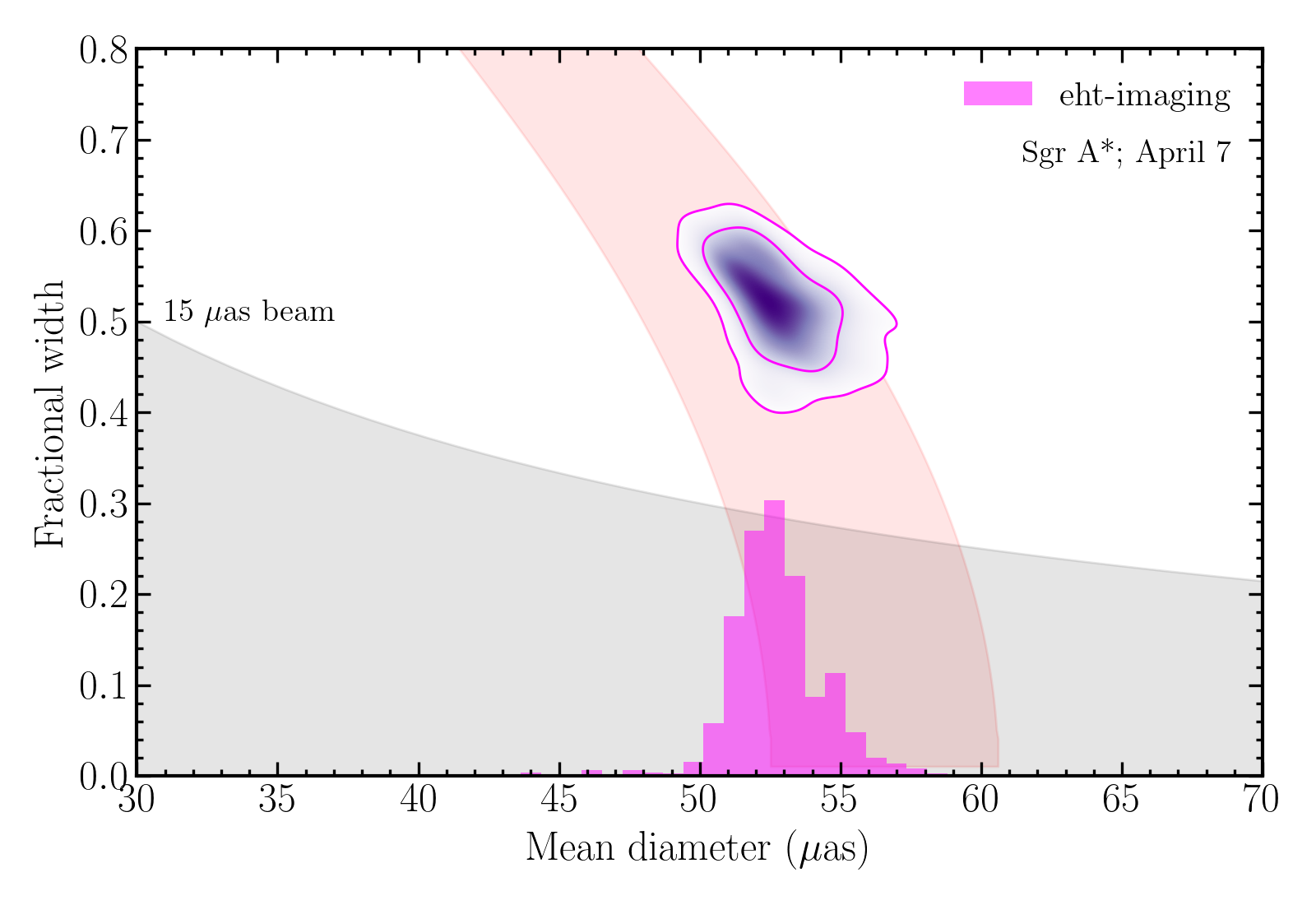
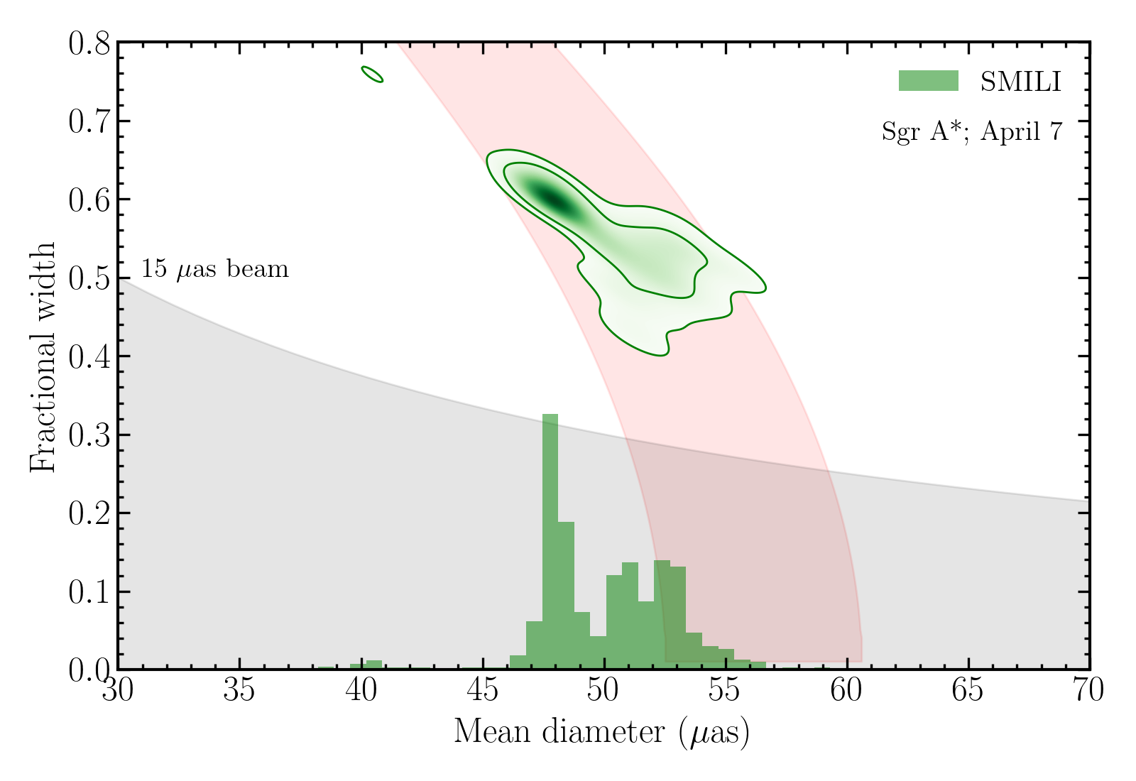
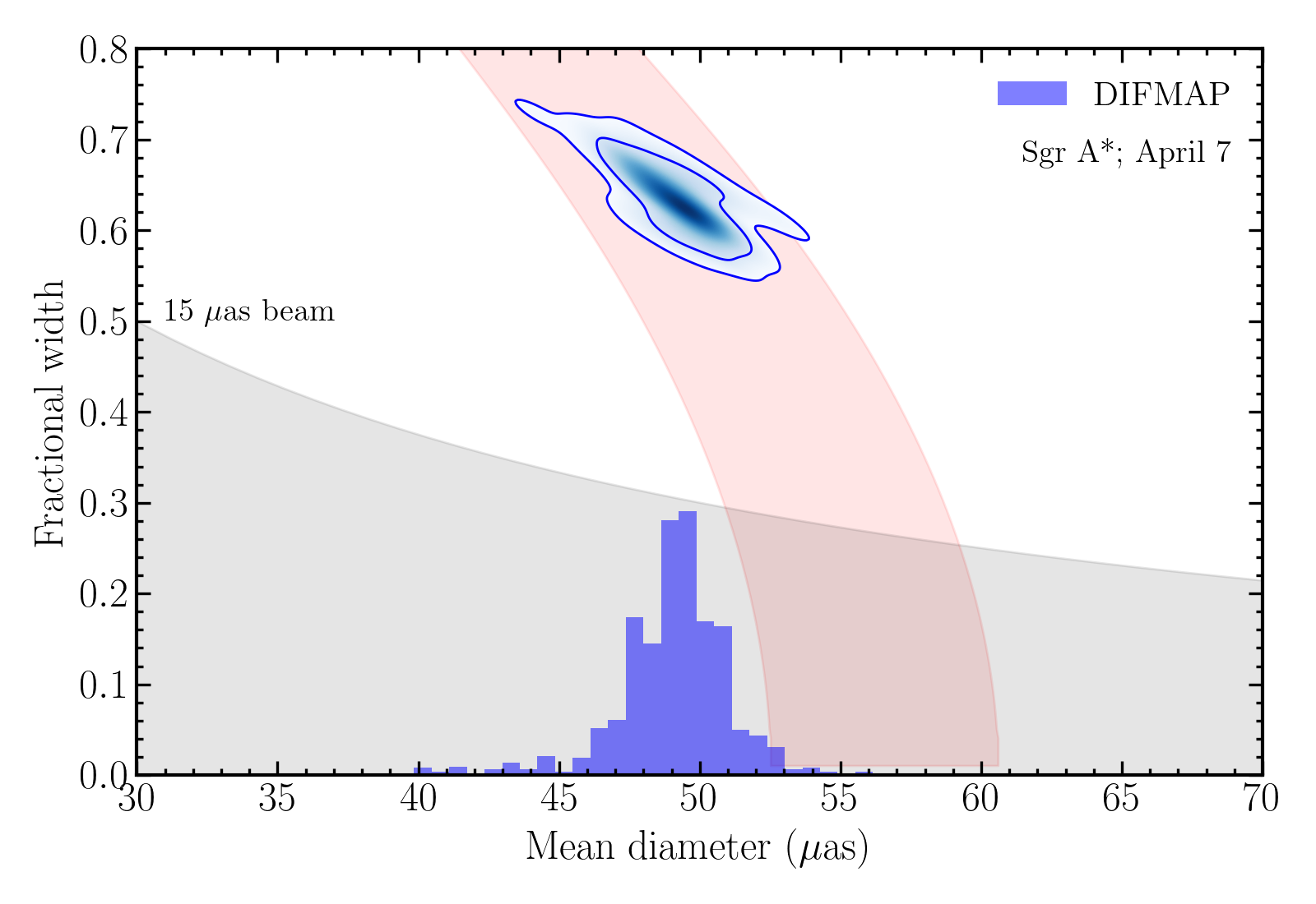
We show in Figure 3 the fractional width and diameter measurements obtained for eht-imaging, SMILI, and DIFMAP top-set images for the April 7 Sgr A^∗ data (see Paper IV for the details of these three imaging algorithms). Even though we apply CHARM to all of the topset images, without employing clustering filters (e.g., to select only ring-like images), we find that the 68th and 95th percentile contours for the ring parameters form compact regions for each algorithm. This indicates that there is a discernible brightness depression in each image that is surrounded by a bright region that has a robust characteristic size.

Figure 5: The fractional ring width and diameter measurements obtained from fitting mG-ring models to the April 7 visibility domain data for Sgr A^∗. The shaded areas are the same as in Figure 4.

The grey bands in Figure 3 mark the effective limit of the fractional width that can be measured with imaging methods because of the finite resolution of the EHT array. The pink bands show the expected anticorrelation between the ring FWHM and the measured diameter $\hat{d}_{\rm m}$ that arises from the Gaussian broadening of an infinitesimally thin ring of diameter $d$. To first order in the fractional ring width, this anticorrelation follows (see Appendix G of Event Horizon Telescope Collaboration et al. 2019a)

$$\hat{d}_{\rm m}=d-\frac{1}{4\ln 2}\frac{{\rm FWHM}^{2}}{d}.$$ (2)

Because some of the inferred fractional widths are relatively large, in calculating the actual shaded areas in Figure 3 we do not make this first-order approximation but rather employ a numerical evaluation of the complete expression.

Figure 6: Selection of simulated $1.3$ mm Sgr A* images for different spacetime geometries and plasma models. From left to right, the upper row presents time-averaged images of a Kerr MAD GRMHD simulation and semi-analytic accretion flow models with the background spacetime given by the JP metric and the Kerr-Sen spacetime, respectively. The bottom row presents images from a covariant MHD simulation of accretion onto a boson star, a covariant MHD simulation of a dilaton black hole, and a semi-analytic accretion flow model from a traversable wormhole spacetime, respectively. Images from top row models were used in the analysis in this study, whereas bottom row models were not used and are shown to provide examples of images from non-Kerr spacetimes and horizonless compact objects. In all cases for which a central brightness depression is present, the size of the ring-like image scales with the boundary of the black-hole shadow.

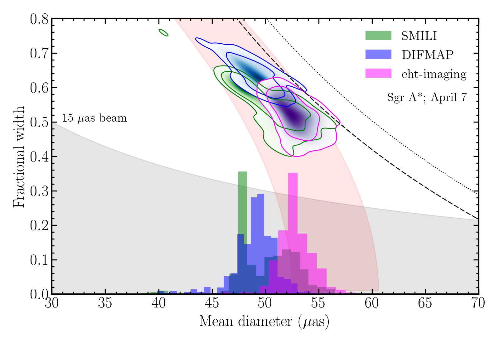
In Figure 4, we compare the fractional widths and mean diameters inferred for Sgr A^∗ with the three imaging algorithms. Even though there appear to be small differences in the mean diameter, all of the contours lie along the expected anticorrelation. This suggests that the differences are simply caused by the various algorithmic choices and do not reflect inconsistencies between them.

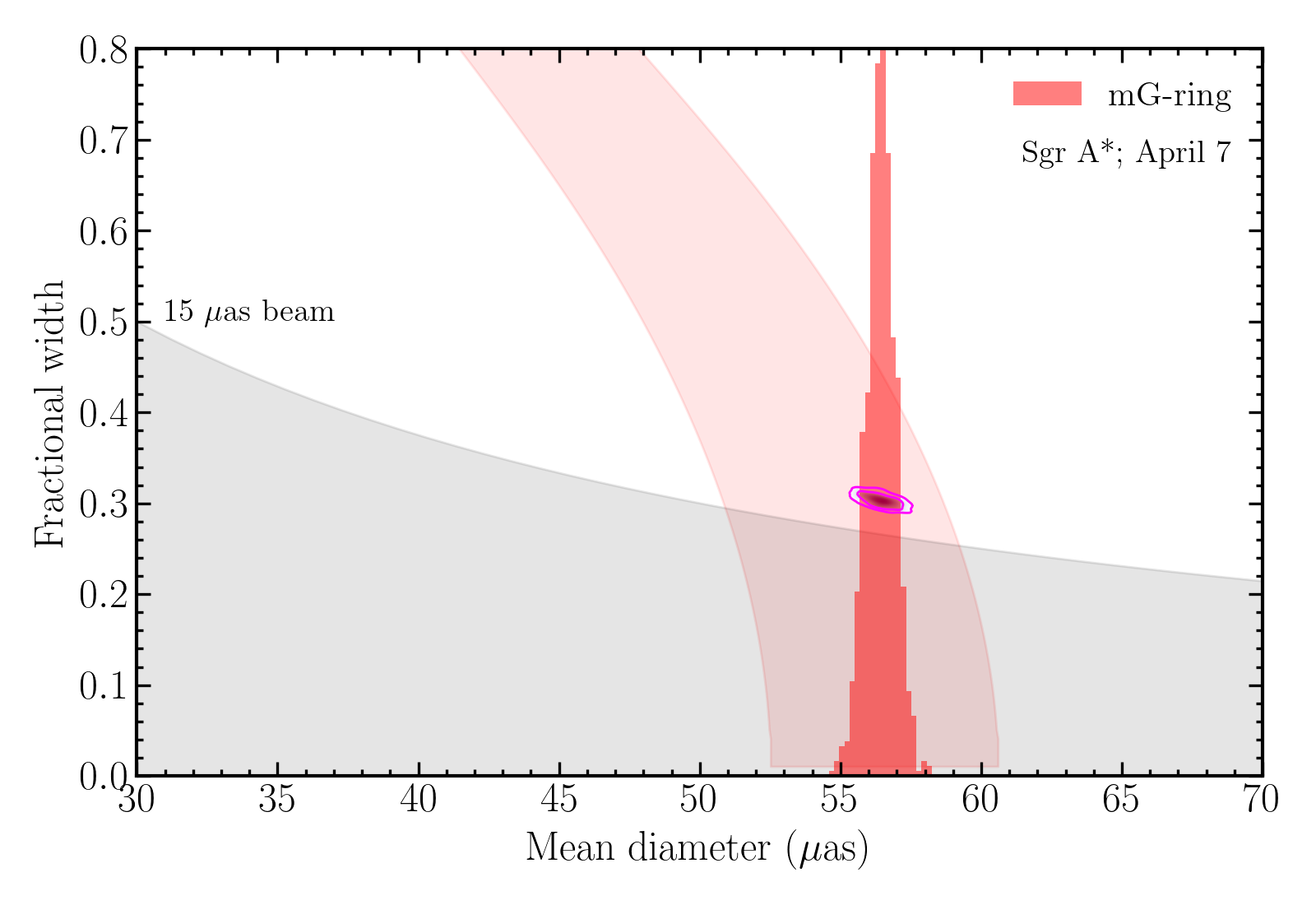
We also use the image diameter and fractional width obtained from fitting analytic models to the visibility data (see Paper IV). In particular, we focus on the mG-ring model described in Paper IV, which comprises a Gaussian broadened ring with flux enhancements on the ring with m-fold azimuthal symmetry and an additional central Gaussian floor component. We use the posteriors obtained from the fitting algorithm Comrade (Tiede, 2022). In Figure 5, we show the posterior over the diameter and the fractional width obtained from fitting the mG-ring model to the April 7 data. The narrow posterior in diameter for this model reflects primarily the insufficient degree of model complexity in the model, as can be seen in the synthetic data analysis below (see also discussion in Psaltis et al. 2020b). Nevertheless, the inferred diameter is consistent with those of the imaging methods, given the expected anticorrelations.

Figure 7: The fractional diameter difference between the diameter of peak emission in the image of a black hole and that of its shadow obtained from three different types of simulations. The blue histogram shows the result from 180,000 snapshots from time-dependent GRMHD simulations in the Kerr metric, spanning a broad range of spins, inclinations, and plasma parameters. The orange histogram shows the same for analytic plasma models in the Kerr metric that relaxes some of the assumptions of the GRMHD simulations, while the green histogram shows the results for analytic plasma models in metrics that deviate from Kerr either parametrically (JP) or through different solutions to the field equations (EMDA). All distributions peak at small positive values.

3.2 The $\alpha_{1}$ Calibration Factor and its Uncertainties

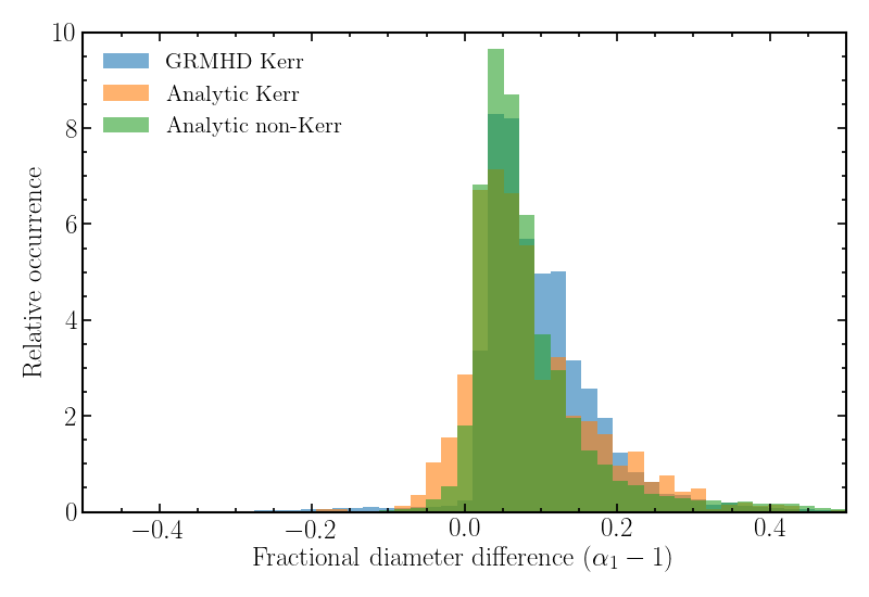
In this section, we use simulated black-hole images to quantify the correction factor $\alpha_{1}$, which is the ratio between the diameter of the peak brightness of the image and the diameter of the black-hole shadow. We employ three different types of models to explore a range of effects releated to the plasma properties, spacetime characteristics, and different numerical realizations of the turbulent flow.

The first category of images comprises $\sim 180,000$ snapshots of GRMHD accretion-flow simulations discussed in Paper V. The simulations cover a range of black-hole spins ($a=-0.94,-0.5,0.,0.5,0.94$), observer inclinations ($i=$10, 30, 50, 70, and 90 degrees), MAD and SANE magnetic field configurations, and thermal electron distributions with temperature prescriptions characterized by $R_{\rm high}=$10, 40, and 160. For each combination in these sets of parameters, we also considered snapshots calculated with two different GRMHD simulation algorithms: KHARMA (Prather et al., 2021) and BHAC (Porth et al., 2017), and corresponding images calculated using two different covariant radiation transport schemes: ipole (Mościbrodzka & Gammie, 2018) and BHOSS (Younsi et al., 2012, 2016).

The second set comprises $\sim 4000$ images from covariant plasma models in the Kerr metric that go beyond some assumptions of GRMHD. These employ analytic calculations that are agnostic to the particular microprocesses responsible for angular momentum transport and particle heating. The particular parameters of these models are discussed in detail in Özel et al. (2021).

The third category includes $\sim 200,000$ images from analytic models that explore a range of black hole metrics that are either parametrically different from the Kerr metric or represent other known solutions to the field equations (Younsi et al., 2021). For the former, we employ the Johannsen-Psaltis (JP) metric (Johannsen & Psaltis, 2011; Johannsen, 2013a), which enables parametric deviations from Kerr and recovers the Kerr spacetime when its deviation parameters vanish, whilst still guaranteeing many of the basic properties of the Kerr metric (i.e., it is Petrov Type-D, free of pathologies, etc). For the latter, we utilize the EMDA (Kerr-Sen) metric (García et al., 1995), which is a solution to the field equations of a modified gravity theory with additional scalar degrees of freedom. The plasma model is the same covariant analytic model of Özel et al. (2021) and the model library spans different black-hole spins, observer inclinations, magnetic field configurations, plasma parameters and, where appropriate, the metric parameters, as discussed in Younsi et al. (2021). We refer to these models as analytic non-Kerr.

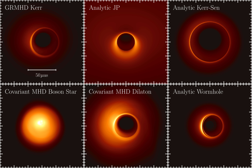
Using the covariant radiation transport code BHOSS (Younsi et al., 2012, 2016), Figure 6 presents a selection of illustrative simulated 1.3 mm Sgr A^∗ images from five different non-Kerr spacetimes, together with an image from a GRMHD simulation of a Kerr black hole. The field of view in all panels is $150~{}\mu\mathrm{as}$ in both directions, with the brightest pixel value in each panel normalized to unity. We show in the top row mean images from covariant MHD simulations averaged over a time window of $5000~{}GM/c^{3}$, with snapshots every $10~{}GM/c^{3}$ ($\sim 3.5$ minutes for Sgr A^∗). The Kerr GRMHD simulation parameters are: MAD magnetic field configuration, $a=0.9375,\,i=30^{\circ},\,R_{\rm low}=1,\,\mathrm{and}\ R_{\rm high}=10$ (see Paper V for further details of the modeling). The upper middle panel shows an image of accretion onto a non-rotating dilaton black hole (Mizuno et al., 2018). The upper right panel presents the image from a simulation of accretion onto a boson star (Olivares et al., 2020; Fromm et al., 2021). The boson star image represents one example of a compact object without an event horizon or an unstable photon orbit, thereby lacking a central brightness depression or a photon ring in its image. We do not consider such configurations in the calibration procedure discussed here but explore them in detail in Section 4.

We present in the bottom row of Figure 6 images from non-Kerr spacetimes with the background semi-analytic accretion flow model as specified in Özel et al. (2021) and Younsi et al. (2021). These spacetimes are the JP and the Kerr-Sen (EMDA) metrics, as well as a spinning traversable wormhole spacetime (Teo, 1998; Harko et al., 2009). The JP metric for this example is non-spinning, with deformation parameters chosen to push the unstable photon orbit very close to the event horizon (hence the smaller central brightness depression). The Kerr-Sen spacetime parameters (axion and dilaton field couplings) have been chosen to produce an image with a photon ring larger than is possible with a Kerr black hole. Finally, the rotating wormhole spacetime is chosen to have a throat radius equal to the event horizon radius of a Kerr black hole with the same spin ($a=0.9375$). In all of the examples with a central brightness depression, the size of the ring-like image scales with that of the black-hole shadow.

We convolve all of the images in the three categories with an $n=2$, 15 G$\lambda$ Butterworth filter to mimic the resolution of the EHT array. We then apply the characterization algorithm CHARM to all of these images to measure the median diameter $D_{\rm im}$ of the bright ring of emission, with respect to the analytically calculated center of the black hole shadow. We also calculate the shadow diameter in each spacetime; for Kerr, we use the analytic approximation derived in Chan et al. (2013). We then define the calibration factor $\alpha_{1}$ as the ratio of the median diameter to the diameter of the shadow. We will refer to the difference $\alpha_{1}-1$ as the fractional diameter difference. If the peak emission in the bright ring coincides with the shadow boundary, then the fractional diameter difference would be equal to zero.

We show in Figure 7 the distribution over the fractional diameter difference for the three types of images. As discussed in Özel et al. (2021) and Younsi et al. (2021), the distribution peaks at small positive values of $\alpha_{1}-1$, indicating that the peak of the bright ring is slightly larger than the boundary of the black hole shadow.

Figure 8: The fractional diameter difference between the diameter of peak emission in ground truth images and the those reconstructed through the three different imaging methods used for EHT analyses. Synthetic data cover 145 sets selected from numerical and analytic Kerr and non-Kerr models, while the image diameters were inferred for all of the top-set images for the image reconstructions of each data set. The small offsets in the calibration parameter mimic those seen in the analysis of the actual Sgr A^∗ data.

Figure 9: The fractional diameter difference between the diameter of peak emission in ground truth images and those reconstructed through fitting the mG-ring model to the visibility domain synthetic data used for EHT analyses.

3.3 The $\alpha_{2}$ Calibration Factor and its Uncertainties

We turn to quantifying the correction factor $\alpha_{2}$ and its uncertainty that arises from applying imaging and model fitting tools to infer the size of a ring-like image. To this end, we first characterized all simulations discussed in Section 3.2 based on image morphology and size, degree of variability, spacetime metric, and plasma model. We then randomly selected segments and snapshots from each category. We assigned a random position angle in the sky to each image and generated synthetic EHT data from them using the VLBI synthetic data generation pipeline SYMBA (Janssen et al. 2019; Roelofs et al. 2020a; Natarajan et al. 2022). SYMBA accounts for the effects of interstellar scattering through the Galactic disk, as well as several realistic atmospheric, instrumental, and calibration effects. In addition, we designated a last category in which synthetic data were generated from a small number of snapshots but with several different realizations of all the measurement uncertainties. This yielded a total of 145 synthetic data sets.

We carried out blind image reconstructions and mG-ring fits to all the synthetic data using the same EHT imaging pipelines as those applied to Sgr A^∗ data, separating into teams who did not have any prior knowledge of the synthetic data characteristics. As for the case of the real data, imaging teams generated a top set of reconstructions for each synthetic data set, using the exact set of algorithmic parameters as those used for the real Sgr A^∗ data. We applied CHARM to the entire top-set image reconstructions (for a total of 145 data sets $\times$ 2000 top-set parameters $\times$ 3 algorithms) as well as to the ground-truth images to measure the calibration factor $\alpha_{2}$. Modeling teams applied the snapshot fitting procedure with an mG-ring model and returned their posteriors for the model diameter, which we used to calculate the $\alpha_{2}$ calibration factor.

In the majority of cases, the set of reconstructions that correspond to the full range of top-set parameters or posteriors yielded a narrow range of diameters and widths for the ring features, indicating a robust inference of the prevalent features with little sensitivity to the choice of regularizers. However, in $<30\%$ of the data sets, the features of the images varied significantly within the topset parameters, leading to an uncertainty in the ring diameter that is $\sim 3-8$ times larger than what is measured in the Sgr A^∗ data (see Fig. 3). This primarily happens when the image size, position angle, and asymmetry of the ground truth image that led to the particular synthetic data set conspire in a way to remove any prominent salient features in the visibility domain and the image reconstruction is dominated by the priors rather than any unique features in the data that an imaging or model fitting algorithm can pick up on. More quantitatively, we define the spread in the diameter for all the reconstructions of a given synthetic data set by using the metric

$${\rm diameter\ spread}=\frac{d_{85}-d_{15}}{d_{50}},$$ (3)

where $d_{85},d_{50}$, and $d_{15}$ refer to the 85th, 50th, and 15th percentile of diameters in a given distribution, respectively. The spread in the top-set reconstructions of the actual Sgr A^∗ data using this metric is $0.06-0.1$ (see Fig 3). We place a conservative limit of diameter spread less than 0.2 for the synthetic data reconstructions and include only the data sets that fulfill this criterion in our derivation of the $\alpha_{2}$ calibration parameters.

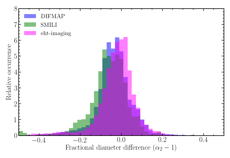
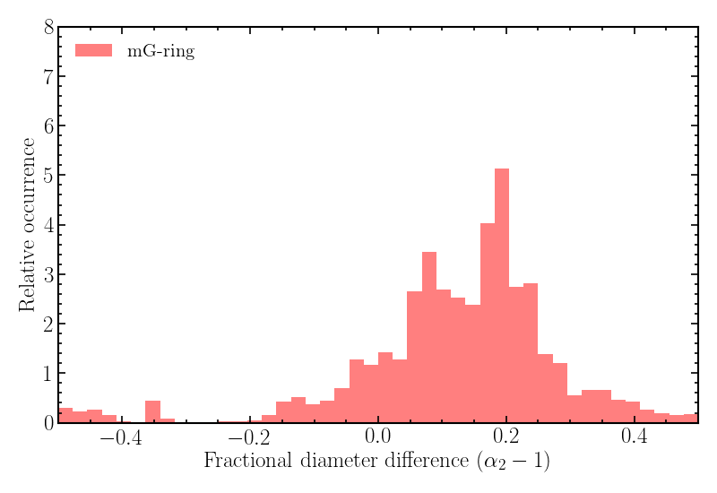
Figures 8 and 9 show the distributions of the fractional diameter difference $\alpha_{2}-1$ for the imaging reconstructions and mG-ring model fits, respectively, of the synthetic data sets discussed above. The trend in Figure 7, i.e., the slight offset between the peaks of the distributions calculated for the different imaging methods, follows the one we see in the reconstruction of the actual EHT Sgr A^∗ data very closely (see Fig. 3). This result reinforces our conclusion that the small differences in the inferred diameters between different algorithms are primarily caused by the different methodologies, prior, and regularizer choices in those methods (see Paper III). The same is true for the trend in the mG-ring results, albeit corresponding to more marked differences.

Figure 10: Posteriors over the shadow diameter inferred using the measurements of the ring diameter size $\hat{d}_{\rm m}$ based on three image-domain algorithms, as well as the two factors $\alpha_{1}$ and $\alpha_{2}$ that quantify the theoretical and measurement calibrations.

Table 1: The Inferred Shadow Diameter of Sgr A^∗ in $\mu$as.

	GRMHD	Analytic	Analytic
		Kerr	non-Kerr
eht-imaging	$48.9_{-5.1}^{+5.2}$	$50.0_{-5.6}^{+5.6}$	$49.9_{-4.9}^{+5.2}$
SMILI	$48.1_{-5.2}^{+6.3}$	$49.1_{-5.7}^{+6.5}$	$49.2_{-5.4}^{+6.2}$
DIFMAP	$46.9_{-5.2}^{+4.9}$	$47.8_{-5.7}^{+5.1}$	$47.8_{-5.2}^{+4.9}$

3.4 The Diameter of the Black-Hole Shadow

We use the combination of the measurements and calibrations discussed in the previous sections to infer the diameter of the boundary of the black hole shadow, $d_{\rm sh}=\hat{d}_{\rm m}/(\alpha_{1}\;\alpha_{2})$. The posterior over the shadow diameter is given by

$$P(d_{\rm sh}|\hat{d}) = C\int d\alpha_{1}\int d\alpha_{2}\;{\cal L}[\hat{d}|d_{\rm sh},\alpha_{1},\alpha_{2}]$$ (4)

$$\qquad\qquad\times P(d_{\rm sh})P(\alpha_{1})P(\alpha_{2})\;,$$

where ${\cal L}[\hat{d}|d_{\rm sh},\alpha_{1},\alpha_{2}]$ is the likelihood of measuring a ring diameter $\hat{d}$ given the model parameters, $P(\alpha_{1})$ and $P(\alpha_{2})$ are the distributions of the calibration parameters, and $C$ is an appropriate normalization constant. $P(d_{\rm sh})$ is the prior over the shadow diameter, which we assume to be flat over a range that is much broader than that of the posteriors.

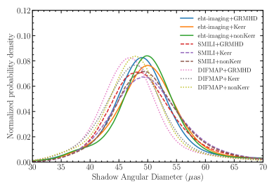
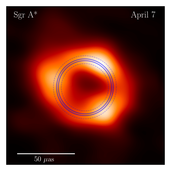
We show in Figure 10 the posteriors over the shadow diameter as inferred from the three image-domain algorithms and for the different theoretical calibrations discussed in Section 3.2. In Table 2, we report the most likely values of the black hole shadow diameter for Sgr A^∗ as well as the 68th percentile credible levels. Finally, in Figure 11, we overlay the inferred shadow boundaries on the average EHT image of Sgr A^∗ obtained from the 2017 April 7 data (Event Horizon Telescope Collaboration et al., 2022b). In this plot, the solid lines show the range $46.9-50.0\;\mu$as of the most likely values and the dashed lines show the envelope of the 68th percentile credible intervals across the different methods, spanning $41.7-55.6\;\mu$as.

Figure 11: Inferred diameter of the black hole shadow boundary overlaid on the average EHT image of Sgr A^∗ obtained from the 2017 April 7 data. Solid lines show the range of most likely values while the dashed lines show the envelope of the 68th percentile credible intervals for all methods.

3.5 Constraints on the Deviation Parameter

Using the uncertainties discussed above, we obtain the posterior over the deviation parameter $\delta$ by

$$P(\delta|\hat{d}) = C\int d\alpha_{1}\int d\alpha_{2}\int d\theta_{\rm g}\;{\cal L}[\hat{d}|\theta_{\rm g},\alpha_{1},\alpha_{2},\delta]$$ (5)

$$\qquad\qquad\times P(\delta)P(\theta_{\rm g})P(\alpha_{1})P(\alpha_{2})\;.$$

Here $C$ is an appropriate normalization constant, ${\cal L}[\hat{d}|\theta_{\rm g},\alpha_{1},\alpha_{2},\delta]$ is the likelihood of measuring a ring diameter $\hat{d}$ given the model parameters, which we identify with the distributions of measurements from the imaging and visibility domain methods, $P(\theta_{\rm g})$ denotes the prior in $\theta_{\rm g}$ given by stellar dynamics measurements, and $P(\alpha_{1})$ and $P(\alpha_{2})$ are obtained from the calibration procedures outlined in Secs. §3.2 and §3.3.

Figure 12: Posteriors on the parameter $\delta$ that measures the deviation of the black hole shadow size obtained for Sgr A^∗ from the Schwarzschild predictions. The top panel uses as a prior the angular size $\theta_{g}$ obtained with Keck observations, while the bottom uses the same quantity from VLT(I). The various curves correspond to different sets of theoretical models used for calibration and the measurements obtained with the various imaging methods. The purple-shaded area shows the $\sim 8$% range predicted for the Kerr metric, depending on the black-hole spin and observer inclination.

Table 2: Schwarzschild Deviation Parameter $\delta$ for Sgr A^∗.

	$\theta_{g}$ Prior	GRMHD	Analytic	Analytic
			Kerr	non-Kerr
eht-	VLT(I)	$-0.08_{-0.09}^{+0.09}$	$-0.05_{-0.11}^{+0.09}$	$-0.07_{-0.09}^{+0.10}$
imaging	Keck	$-0.04_{-0.10}^{+0.09}$	$-0.02_{-0.11}^{+0.11}$	$-0.02_{-0.09}^{+0.10}$
SMILI	VLT(I)	$-0.10_{-0.10}^{+0.12}$	$-0.08_{-0.11}^{+0.13}$	$-0.08_{-0.10}^{+0.12}$
	Keck	$-0.06_{-0.10}^{+0.13}$	$-0.04_{-0.11}^{+0.13}$	$-0.04_{-0.10}^{+0.13}$
DIFMAP	VLT(I)	$-0.12_{-0.08}^{+0.10}$	$-0.10_{-0.10}^{+0.09}$	$-0.10_{-0.09}^{+0.09}$
	Keck	$-0.08_{-0.09}^{+0.09}$	$-0.07_{-0.11}^{+0.10}$	$-0.07_{-0.09}^{+0.09}$
mG-ring	VLT(I)	$-0.17_{-0.10}^{+0.11}$	$-0.14_{-0.13}^{+0.10}$	$-0.17_{-0.09}^{+0.13}$
	Keck	$-0.13_{-0.11}^{+0.11}$	$-0.12_{-0.11}^{+0.11}$	$-0.12_{-0.11}^{+0.10}$

Figure 13: Same as Fig. 12 but for the measurements obtained from fitting mG-ring to the visibility domain data.

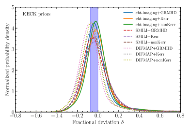
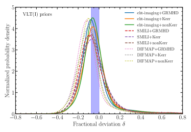
As discussed earlier, we consider two separate priors for $\theta_{\rm g}$ denoted by Keck and VLTI, three different measurements of the ring diameter from imaging methods (together with their corresponding $\alpha_{2}$ calibrations) denoted by eht-imaging, SMILI, and DIFMAP, as well as three different sets of snapshot images for the $\alpha_{1}$ calibration denoted by GRMHD, Analytic Kerr, and Analytic JP. We assume a flat prior in the fractional deviation $\delta$, with limits that cover a range that is sufficiently broad not to affect the posteriors. We perform the two integrals in eq. (5) numerically and show the resulting posteriors in the deviation parameter $\delta$ in Figure 12.

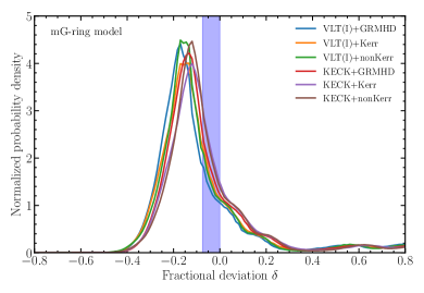
We repeat the same procedure for the measurements obtained from mG-ring fits to the Sgr A^∗ data. We show the corresponding result for the deviation parameter $\delta$ in Figure 13.

We present in Table 2 the means and 68th percentile credible levels for the posteriors we obtain for the deviation parameter $\delta$ using different combinations of black hole mass priors, theoretical models used for calibration, as well as the imaging and model-fitting methods used on the Sgr A^∗ data. All of the posteriors are consistent with each other and with no deviation from the General Relativistic predictions, we choose the eht-imaging +Keck+GRMHD and eht-imaging +VLTI+GRMHD combinations as the two fiducial cases to calculate constraints on the individual metric parameters in the remainder of this paper.

4 Are there Viable Alternatives to an Event Horizon?

While there is overwhelming evidence that Sgr A^∗ contains a large amount of mass confined within a very small volume, the question of whether it is a true black hole remains unresolved. The defining characteristic of a black hole is the presence of an event horizon. While it is relatively easy to show that observations of Sgr A^∗ are consistent with the presence of an event horizon (e.g., the many black hole based models discussed in Paper V), proving that all alternatives are ruled out is well-nigh impossible. Here we discuss what EHT observations of Sgr A^∗ are able to add to this question.

If Sgr A^∗ does not have an event horizon, it is likely to have some kind of a surface. Alternatively, the object might be a boson star, naked singularity, or some other exotic solution of gravitational physics (see Cardoso & Pani 2019 for a review of exotic compact object models). If we could rule out some of these possibilities using observational data, then the case for Sgr A^∗ having an event horizon would become significantly stronger. We discuss below two arguments against Sgr A^∗ possessing a radiating surface. One argument (Section 4.1) is well-developed in the literature (Narayan et al., 1998; Narayan, 2002; Broderick & Narayan, 2006, 2007; Narayan & McClintock, 2008; Broderick et al., 2009), while the other (Section 4.2) is new. Models involving boson stars and certain kinds of naked singularities are considered in Section 4.3, and other exotic possibilities, including wormholes, are discussed in Section 5.2.

4.1 Thermalizing Surface

Accretion in Sgr A^∗ is believed to occur via a hot accretion flow (Yuan & Narayan, 2014). Now that the EHT image of Sgr A^∗ (Paper III) has revealed a brightness temperature well in excess of $10^{9}$ K, the evidence for the presence of very hot gas is particularly compelling.

The radiative luminosities of hot accretion flows are generally far less than $\dot{M}c^{2}$ (Narayan et al., 1995; Yuan & Narayan, 2014), where $\dot{M}$ is the mass accretion rate. Therefore, the accreting gas in these systems reaches the compact object at the center with a considerable amount of thermal and kinetic energy. If the compact object is a black hole, this energy simply disappears through the event horizon. On the other hand, if the object has a surface, the energy will be thermalized and re-radiated (once the system reaches steady state), giving a large surface luminosity that should be visible to a distant observer. Observations can thus tell the difference between an event horizon and a thermalizing surface.

In the previous paragraph, and also in the rest of Section 4, we assume that (i) matter in the compact object at the center of Sgr A^∗ satisfies energy conservation, (ii) that it obeys the laws of thermodynamics, in particular, that it approaches statistical equilibrium in steady state, and (iii) that it couples to and radiates in all electromagnetic modes. These assumptions can be considered "natural" minimal principles, but they can be violated in extreme models. For example, the shell-like black hole mimicker described in Danielsson et al. (2021) can be designed either not to produce any electromagnetic radiation, or to radiate only in a handful of modes, thereby violating assumption (iii). It is not possible to constrain such models using astronomical observations in electromagnetic bands, though in certain cases it may be possible to distinguish them via gravitational waves (Abbott et al., 2021) (e.g., Chirenti & Rezzolla, 2007, for the case of gravastars). Note that even very exotic objects would satisfy our assumptions, including (iii), if only a small fraction of the accreted baryonic gas survives on their surface as normal matter. To be optically thick in the electromagnetic bands of interest to us, the skin of normal matter should have a surface density as little as $1\,{\rm g\,cm^{-2}}$, which corresponds to just $10^{-14}$ of the total mass of Sgr A^∗. An exotic object would need to convert all accreted gas on its surface to electromagnetically-inactive material if it is to escape detection by electromagnetic observations.

For a spherically symmetric spacetime, matter that starts from rest at infinity and then accretes via a radiatively inefficient mode to come to rest on a surface at radius $R_{*}$, will release thermal energy as measured at infinity equal to a fraction $\eta$ of the rest mass energy of the gas, where (the following expression is obtained for the Schwarzschild metric, Broderick & Narayan 2006),

$$\eta=1-\left(1-\frac{2M}{R_{*}}\right)^{1/2}\gtrsim\frac{M}{R_{*}},$$ (6)

and we use geometrized units: $G=c=1$. If the released thermal energy is radiated back to infinity – we emphasize that this is unavoidable once the object reaches steady state – the extra luminosity from the thermalizing surface will be typically much larger than the luminosity radiated by the hot accretion flow itself. This feature can be exploited to distinguish black holes, which by definition have an event horizon, from other kinds of compact object that have a surface. In the context of stellar-mass black holes, this argument provides a convenient way of distinguishing black holes from neutron stars (Narayan & Yi, 1995; Narayan et al., 1997; Garcia et al., 2001; Done & Gierliński, 2003; McClintock et al., 2004, see Narayan & McClintock 2008 for a review).

In the case of Sgr A^∗, the argument proceeds differently. In essence, the observed sub-millimeter radiation provides a lower limit on the mass accretion rate, $\dot{M}_{\rm min}$, regardless of whether the radiation is produced by inflowing hot gas or an outflowing jet. Therefore, given an assumed radius $R_{*}$ of the surface, we can estimate the minimum surface luminosity that should be observed at infinity,

$$L_{\infty}>\eta\dot{M}_{\rm min}c^{2}.$$ (7)

As we show below, the surface radiation should appear in the infrared, where observations provide strong upper limits on the luminosity of Sgr A^∗. These limits lie far below the predicted minimum surface luminosity, implying that Sgr A^∗ does not have a radiating surface. Versions of this argument have been made in previous papers in the context of Sgr A^∗ (see Narayan & McClintock, 2008, for a review). A similar argument also applies to the supermassive black hole in M87 (Broderick et al., 2015; Event Horizon Telescope Collaboration et al., 2019c). In related work, Lu et al. (2017) argued that the absence of flashes of radiation from stars crashing on supermassive black hole candidates in galactic nuclei requires these candidates to be true black holes with event horizons.

4.1.1 EHT Limit on the Radius of the Surface

In the case of Sgr A^∗, a somewhat weak link in the argument outlined above was the hitherto lack of a strong upper limit on the radius $R_{*}$ of a putative surface in Sgr A^∗. Since the surface luminosity for a given $\dot{M}$ scales as $L_{\infty}\propto\dot{M}(M/R_{*})$ (Equations 6 and 7), one could make the predicted luminosity small by arbitrarily increasing $R_{*}/M$, thereby evading observational limits. This loophole has now been closed by EHT observations.

Using a maximally conservative analysis of EHT 2017 visibility data, and without any model assumptions, Paper II estimates the FWHM of the image of Sgr A^∗ to lie in the range $39-87\,\mu$as. With a conversion factor, $GM/c^{2}D\approx 5\,\mu$as (see Figure 1), this corresponds to an image diameter $<18M$.

The observed 230 GHz radiation in Sgr A^∗ is from the hot accretion flow, not from the surface (which should radiate in the infrared). Any surface must lie interior to the 230 GHz-emitting hot accretion flow and should have an apparent diameter smaller than $18M$. Thus, from the analysis in Paper II, we set the following upper limit on the apparent radius of the surface as viewed by a distant observer: $R_{\rm app}<9M$.

Paper III presents image reconstructions of Sgr A^∗ based on the EHT 2017 data. Table 7 in that paper summarizes the results of fitting a ring model to image reconstructions based on several methods. Using the imaging results from DIFMAP, eht-imaging and SMILI, and combining the ring analyses with REx and VIDA (see Paper III for details), the average ring diameter estimate is $d=51.3\pm 2.0\,\mu$as, and the ring width estimate is $w=29.6\pm 3.6\,\mu$as (these results correspond to descattered images from April 7 data). We take $(d+w)=80.9\pm 4.1\,\mu$as as a reasonable proxy for the apparent outer diameter of the source. Using the 95% confidence upper limit, $(d+w)<88\,\mu$as, we obtain $R_{\rm app}<8.8M$ (95%cl). Paper III obtains a tighter constraint using the Bayesian imaging method Themis, while Paper IV similarly reports tighter constraints by fitting mG-ring models (based on Johnson et al. 2020) directly to visibility data. To be conservative, we do not use these limits.

The analyses described in the previous paragraph treat $d$ and $w$ as uncorrelated quantities. However, as the careful analysis in Section 3.1 of the present paper shows, there is a strong anti-correlation between the estimated values of $d$ and $w$, such that their sum $(d+w)$ is quite tightly constrained. The dotted and dashed curves in Figure 4 correspond to $(d+w)=90\,\mu$as and $80\,\mu$as, or equivalently, $R_{\rm app}=9M$ and $8M$, respectively. Clearly, from this analysis, $R_{\rm app}<8M$ is a safe upper limit (at about 95% confidence).

To be very safe, we choose as a conservative upper limit on the apparent radius of a surface in Sgr A^∗, $R_{\rm app}<9M$. For a Schwarzschild spacetime, gravitational deflection of rays causes the apparent radius of a spherical surface as viewed by an observer at infinity to be larger than the true areal radius $R_{*}$. The relation between the two is

$$R_{\rm app} = 3\sqrt{3}M,\qquad\qquad\qquad R_{*}\leq 3M,$$ (8)

$$= R_{*}\left(1-\frac{2M}{R_{*}}\right)^{-1/2},~{}R_{*}>3M.$$

Our upper limit, $R_{\rm app}<9M$, then corresponds to $R_{*}<8M$. In the discussion below, we consider the full range of allowed $R_{*}$ values, from the event horizon radius $R_{H}=2M$ to the upper limit, namely, $2M<R_{*}\leq 8M$.

4.1.2 Predicted Spectrum of Surface Radiation

Paper V discusses hot accretion flow models of Sgr A^∗ based on extensive GRMHD simulations. The models indicate that the mass accretion rate in Sgr A^∗ is typically $\dot{M}\sim 10^{-8}M_{\odot}{\rm yr^{-1}}$ (similar to estimates reported in, e.g., Falcke et al. 1993; Yuan et al. 2003; Chael et al. 2018; Ressler et al. 2020), but with a broad distribution that extends from $\dot{M}_{\rm min}\sim 10^{-9}M_{\odot}{\rm yr^{-1}}$ to $\dot{M}_{\rm max}\sim 10^{-6}M_{\odot}{\rm yr^{-1}}$. The models at the lower end of this range are actually ruled out by various constraints (see Paper V); nevertheless, we stick to $\dot{M}_{\rm min}=10^{-9}M_{\odot}{\rm yr^{-1}}$ as a safe and conservative lower limit on the mass accretion rate. Equations (6) and (7), combined with our upper limit on $R_{*}$, then show that the surface luminosity measured at infinity must be $\gtrsim 10^{37}~{}{\rm erg\,s^{-1}}$.

Meanwhile, we know that the hot accretion flow in Sgr A^∗ produces synchrotron radiation at sub-millimeter wavelengths with a luminosity $\sim 5\times 10^{35}{\rm erg\,s^{-1}}$, shown by the green curves in Figure 14. Even in the absence of any independent estimate of $\dot{M}$, just the fact that accretion results in this much radiation implies a certain minimum energy flow on to the surface. Since the accreting gas generally moves radially inward, relativistic beaming causes more radiation to impinge on the central object compared to what escapes to infinity. Thermalization of this infalling radiation would then give a surface luminosity greater than $5\times 10^{35}{\rm erg\,s^{-1}}$. Any additional energy released by the mechanical and thermal energy of the infalling gas (this is expected to dominate in most scenarios) would further increase the surface luminosity. We therefore treat $5\times 10^{35}{\rm erg\,s^{-1}}$ as an even more conservative lower bound on the surface luminosity of Sgr A^∗ than that discussed in the previous paragraph.

A key feature of radiation emitted from a central surface in a hot accretion flow is that it will appear in a different region of the electromagnetic spectrum than the emission from the hot accreting gas and jet. The latter dominates in the radio and sub-millimeter bands (Figure 14, green curves). Meanwhile, the radiating gas at the surface, being optically thick, will radiate like a blackbody to a very good approximation (McClintock et al. 2004, Broderick & Narayan 2006, 2007).

The temperature of this radiation, measured at infinity, is given by

$$T_{\infty} = \left(\frac{L_{\infty}}{4\pi R_{\rm app}^{2}\sigma_{\rm SB}}\right)^{1/4}$$ (9)

$$\approx 2100\,{\rm K}\left(\frac{L_{\infty}}{10^{36}\,{\rm erg\,s^{-1}}}\right)^{1/4}\left(\frac{9M}{R_{\rm app}}\right)^{1/2},$$

where $\sigma_{\rm SB}$ is the Stefan-Boltzmann constant. For the estimates of $L_{\infty}$ and $R_{\rm app}$ derived earlier, the predicted radiation should be in the near-infrared and optical bands. If we define the characteristic frequency $\nu_{*}$ of the blackbody radiation by $h\nu_{*}=kT_{\infty}$, the spectral energy distribution (SED) at infinity takes the form

$$\nu L_{\nu}=\frac{15}{\pi^{4}}\,L_{\infty}\frac{(\nu/\nu_{*})^{4}}{\exp(\nu/\nu_{*})-1},\quad\nu_{*}\equiv\frac{kT_{\infty}}{h}.$$ (10)

Figure 14: Left: Predicted spectral energy distributions (SEDs), $\nu L_{\nu}$ vs $\nu$, of thermal radiation from Sgr A^∗, if the object has a thermalizing surface with radius $R_{*}=2.5M$ (selected as a fiducial model). Three choices of the mass accretion rate on the surface, $\dot{M}=[10^{-7},~{}10^{-8},~{}10^{-9}]\,M_{\odot}{\rm yr^{-1}}$, are shown as solid black curves. The dashed blue curve corresponds to a model with a surface luminosity of $5\times 10^{35}{\rm erg\,s^{-1}}$, a conservative lower bound. Observational data in various wavebands are plotted as solid circles. The thick red line and large green filled circle correspond to the 5th percentile of the variable infrared emission (Witzel et al., 2018; Gravity Collaboration et al., 2020b), which we treat as an upper limit on any quiescent infrared luminosity from a potential surface in Sgr A^∗. This upper limit from the observations lies well below the theoretical SEDs, and therefore rules out these models. The green curve on the left is an empirical fit to the radio and sub-millimeter part of the observed SED; the radiation in this region of the spectrum is produced by synchrotron emission from the hot accretion flow, and the corresponding luminosity is $\sim 5\times 10^{35}{\rm erg\,s^{-1}}$. Right: Theoretical SEDs of surface emission from an accretion flow in Sgr A^∗ with $\dot{M}=10^{-9}M_{\odot}{\rm yr^{-1}}$ falling on surfaces of radii, $R_{*}=[2M,~{}3M,~{}4M,~{}6M,~{}8M]$, respectively (solid black lines). All the SEDs are inconsistent with infrared observations (thick red line, large green filled circle). Hence these models are ruled out.

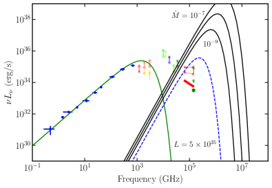
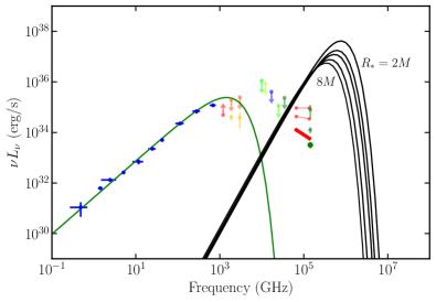
The left panel in Figure 14 shows predicted SEDs of surface radiation from Sgr A^∗, if the object has a surface with a radius $R_{*}=2.5M$; we choose this radius as a fiducial model for illustration. The three solid black curves correspond to mass accretion rates $\dot{M}=[10^{-7},~{}10^{-8},~{}10^{-9}]~{}M_{\odot}{\rm yr^{-1}}$, respectively, the last of which is the conservative lower limit from Paper V mentioned earlier. The dashed blue curve corresponds to the absolute lower limit on the surface luminosity, $L_{\infty}=5\times 10^{35}{\rm erg\,s^{-1}}$, discussed above.

The right panel in Figure 14 shows another sequence of models in which we vary the surface radius $R_{*}$. Taking the previously mentioned conservative mass accretion rate estimate of $10^{-9}M_{\odot}{\rm yr^{-1}}$, we consider surface radii $R_{*}=[2M,~{}3M,~{}4M,~{}6M,~{}8M]$, respectively.

In all the models shown in the two panels in Figure 14, the predicted surface emission (black and blue curves) is spectrally well separated from the synchrotron emission of the hot accretion flow (green curve).

Therefore, this predicted signature of surface emission is easy to identify via observations, making it possible to develop a robust test for the presence of a thermalizing surface.

4.1.3 Observational Limit on Surface Luminosity

Observations of Sgr A^∗ have improved substantially in recent years. The current status is summarized in Section 2.2 and Figure 2, and the data are shown again in Figure 14. The infrared data are of most interest to us and are highlighted by the red line segments and green filled circles, which correspond to the 5th (thick red line and large green filled circle at the bottom), 50th (thin line, small circle), and 95th (thin line, small circle) percentiles, respectively, of the variable infrared luminosity. Sgr A^∗ exhibits frequent flares in its infrared light curve (Eckart et al., 2004b; Eisenhauer et al., 2005; Hora et al., 2014; Witzel et al., 2018), which are interpreted as transient electron heating events in the hot accretion flow or jet. A few bright flares have been shown to come from gas orbiting the central object at a projected radius $R_{\rm flare}\sim 6-10M$ (Gravity Collaboration et al., 2018b). This location is not very different from the region of the flow that produces the sub-millimeter radiation observed by the EHT.

If Sgr A^∗ were an object with a thermalizing surface, then given its large mass we would expect it to have an enormous thermal capacity. Consequently, thermal emission from its surface is not expected to show violent flaring activity. The observed infrared flares are thus much more likely to be produced by the hot accretion flow, possibly in transient turbulent heating or magnetic reconnection events (Markoff et al., 2001; Yuan et al., 2004; Ball et al., 2016; Ressler et al., 2017; Davelaar et al., 2018; Dexter et al., 2020; Nathanail et al., 2020, 2021; Chatterjee et al., 2021; Porth et al., 2021; Ripperda et al., 2021; Ball et al., 2021).

Since any surface infrared emission in Sgr A^∗ must be steady, we ignore the fluctuating flare emission and treat the 5th percentile (the thick red line and large filled green circle in Figure 14) as the maximum steady infrared emission from a surface. Note that Paper V uses an upper limit of $\nu L_{\nu}<10^{34}{\rm erg\,s^{-1}}$ in infrared (50th percentile) when evaluating their GRMHD-based accretion-jet models. As Figure 14 shows, this upper limit (especially the large green filled circle) lies nearly two orders of magnitude below the strict lower bound on the predicted surface luminosity discussed earlier (dashed blue line), and three orders of magnitude below predictions of more realistic models (solid black lines). We thus conclude that Sgr A^∗ cannot have a thermalizing surface with characteristics similar to any of the models considered in Figure 14, ergo the case for an event horizon is much strengthened.

4.1.4 Discussion and Caveats

Compared to previous discussions of this topic, what has improved is that, thanks to the EHT image of Sgr A^∗, we are now able to limit ourselves safely to surface radii $R_{*}<8M$, whereas in earlier works much larger radii were considered (as large as $1000M$ in Narayan 2002, and $100M$ in Broderick et al. 2009). Moreover, the infrared constraints are also now very much stronger (Figure 14). Correspondingly, the argument for the absence of a thermalizing surface is substantially strengthened.

The discrepancy between the maximum steady infrared luminosity that Sgr A^∗ can possibly have (the 5th percentile thick red line and large green circle in Figure 14) and the minimum possible luminosity it could theoretically have and still possess a thermalizing surface (the dashed blue line) is too large to be circumvented with small fixes to model details. This statement is true even if we use the 50th percentile of the infrared observations (the middle red line and middle green circle in Figure 14), which would be equivalent to counting all the observed infrared radiation, including the flares, as surface emission. If we wish to consider models of Sgr A^∗ with a surface, we have to find a weakness in one of the links in the underlying logic of the argument. An easy way out is to give up one of the basic physics assumptions listed in the third paragraph of Section 4.1. Here we consider other less-drastic possibilities.

Could the predicted infrared radiation from a hypothetical surface in Sgr A^∗ be obscured by foreground matter such as dust? This is highly unlikely since the radiation from the infrared flares is clearly visible, and that radiation comes from hot external gas (not from the surface) at radii within $10M$ (Gravity Collaboration et al., 2018b). It is hard to imagine an obscuring medium that allows flare emission to make it through but blocks radiation from the surface.

Another minor worry may be quickly dealt with. Because of spacetime curvature, radiation from a surface at areal radius $R_{*}$ in a Schwarzschild spacetime takes longer to reach a distant observer compared to a ray that travels in flat spacetime. Could this delay be so large that surface radiation has not yet reached us? Let us write

$$R_{*}=(1+\mu)R_{H},$$ (11)

where $R_{H}=2M$ is the radius of the event horizon. For $\mu\ll 1$, the additional time delay is $\sim 2M\ln(1/\mu)$, which is $\sim 40\,\ln(1/\mu)$ s in the case of Sgr A^∗. Even if the logarithm is as large as $100$ (corresponding to $R_{*}$ being located a Planck length above the event horizon), the extra time delay is only about an hour.

A related worry is that the gravitational redshift, $(1+z)\sim\mu^{-1/2}$, between the surface and infinity might dilute the observed luminosity sufficiently to make the surface radiation invisible. Abramowicz et al. (2002) noted that this effect causes the radiation luminosity that reaches the observer to be reduced by a factor of $1/(1+z)^{4}\sim\mu^{2}$ compared to what is emitted at the surface. They claimed that, if $(1+z)$ were large enough, no detectable radiation would reach the observer and it would be impossible to distinguish an event horizon from a surface.

However, gravitational redshift is not an issue for the line of argument we have presented in this paper because we expressed everything in terms of energy and luminosity as measured at infinity; in such a framework, all redshift factors drop out. For instance, if the radiation observed at infinity has a temperature $T_{\infty}$, then the radiation emitted by the surface will have a temperature $T_{\rm local}=(1+z)T_{\infty}$ in the local rest frame. The radiation emerging from the surface will have a flux equal to $\sigma_{\rm SB}T_{\infty}^{4}(1+z)^{4}$, and the corresponding luminosity is larger than what reaches infinity by precisely the factor of $(1+z)^{4}$ noted by Abramowicz et al. (2002). The only question is whether the system has enough time to heat up to such a high local temperature. We discuss this important issue next.

Sgr A^∗ is presumably as old as the Milky Way Galaxy, i.e., several billion years old. Over much of that time, it must have accreted gas at a rate equal at least to the present $\dot{M}$. The time needed to achieve the steady state condition implicit in equation (9), namely, $\eta\dot{M}c^{2}=L_{\infty}=(\sigma T_{\infty}^{4})(4\pi R_{\rm app}^{2})$, or equivalently $T_{\rm local}=(1+z)T_{\infty}$, is far shorter than the age of Sgr A^∗ for almost any model.

The one exception is if $\mu\ll 1$, i.e., if the surface $R_{*}$ is extremely close to the event horizon. In this limit, as Lu et al. (2017) argued, the time required to achieve steady state scales as $\mu^{-1}$ and can become arbitrarily long. The physical reason is that the region between $R=R_{*}$ and the photon sphere, $R_{\rm ph}=3M$, traps radiation. This volume has a large thermal capacity, and therefore takes a long time to reach steady state. Applying this logic to Sgr A^∗, Lu et al. (2017) concluded that the absence of infrared radiation in Sgr A^∗ rules out a thermalizing surface only if $\mu\gtrsim 10^{-14}$. If the surface is even closer to the horizon radius than this limit, i.e., if $R_{*}\lesssim R_{H}+10^{-2}$ cm, then the steady state condition will be invalid. Their argument thus provides an upper limit on $R_{*}$.

Using completely different reasoning, Carballo-Rubio et al. (2018) set a lower limit on $\mu$. The argument goes as follows. Because Sgr A^∗ accretes mass continuously, its horizon radius $2M$ increases with time. In order to maintain $R_{*}=(1+\mu)R_{H}$, the surface also needs to expand. However, if $\mu$ is too small, the required expansion speed is greater than the speed of light in the local frame, which is unphysical. Using a conservative estimate of $\dot{M}\sim 10^{-11}M_{\odot}{\rm yr^{-1}}$ (which is two orders of magnitude smaller than the lower limit given in Paper V and more than seven orders of magnitude less than the likely average accretion rate over the life of Sgr A^∗), Carballo-Rubio et al. (2018) conclude that Sgr A^∗ can avoid the faster-than-light conflict only if $\mu\gtrsim 10^{-23}$, i.e., if $R_{*}\gtrsim R_{H}+10^{-11}$ cm. Note that this rules out models in which the surface lies a Planck length ($10^{-33}$ cm) above the event horizon, as gravastar models (Mazur & Mottola, 2001; Chapline, 2003) often implicitly assume.

Combining the arguments in the previous two paragraphs, we are left with an interesting class of models with $\mu$ in the range $10^{-23}<\mu<10^{-14}$ for which Sgr A^∗ is presently allowed to have a thermalizing surface and yet not be ruled out by infrared constraints. This gap in model space merits further investigation.

Another issue worth serious discussion is the assumption that the surface will radiate like a blackbody. Since we are considering an object which (i) is in steady state and therefore in thermal equilibrium (by our assumptions), (ii) is likely nearly isothermal in the sense that the redshifted temperature $T_{\infty}$ is independent of radius inside the object, and (iii) has an enormous optical depth, it seems unavoidable that the emission must be close to a blackbody. (For instance, stars radiate roughly like blackbodies because of their large optical depths, and would be perfect blackbodies if they were isothermal.) Any deviations from a perfect blackbody in the putative surface radiation in Sgr A^∗ might thus be expected to be minor. However, the specific case of radiation produced by energy release from matter falling on the surface of a compact supermassive ($>10^{6}M_{\odot}$) object has not been studied and merits further attention. Models of spherical accretion on neutron stars ($M=1.4M_{\odot}$) studied by Shapiro & Salpeter (1975) suggest that modest deviations from a perfect blackbody are expected in that case; their models show some hardening of the thermal spectrum plus the appearance of a power-law spectral component extending to higher frequencies. If the corresponding effects in the case of a surface in Sgr A^∗ ($M=4\times 10^{6}M_{\odot}$) are similarly modest, then our blackbody assumption is quite safe. Note that Shapiro & Salpeter (1975) did not include ray deflections and strong lensing in their model.

The argument for a blackbody spectrum is very strong in one particular limit. When the surface has a radius $R_{*}$ close to $R_{H}$, i.e., $\mu\ll 1$, the volume between $R_{*}$ and $R_{\rm ph}=3M$ acts like an enclosed cavity, with radiation allowed to escape only over a small solid angle $\sim\mu$. The cavity then behaves like a textbook isothermal “furnace” with a tiny pinhole for escaping radiation. In this limit, the radiation that reaches a distant observer will be indistinguishable from a perfect blackbody (Broderick & Narayan, 2006).

If the quiescent infrared radiation in Sgr A^∗ corresponds to blackbody emission from a surface, it should be completely unpolarized. On the other hand, if the radiation is produced by synchrotron emission in optically thin (weak) flares, we might expect a certain degree of linear polarization. Bright infrared flares in Sgr A^∗ show clear evidence for strong linear polarization (Eckart et al., 2006; Gravity Collaboration et al., 2020c), but there is presently no information on the degree of polarization of the weak emission below the 5th percentile. Sensitive polarimetry could be used in the future to explore this regime, and might help to reduce even further the maximum level of blackbody emission allowed in Sgr A^∗.

4.2 Reflecting Surface

In this Subsection, we focus again on the possibility that Sgr A^∗ may have a surface, but now we explore models in which the surface reflects incident radiation. We assume that, in the rest frame of the surface at some fixed areal radius $R_{*}$, the following properties hold: (i) Any inward-moving ray that is incident with wave-vector $k^{\mu}$ becomes an outward-moving ray with $k^{r}$ reversed and the other components of $k^{\mu}$ unchanged. (ii) If the intensity of the incoming ray is $I_{\nu}$, the outgoing ray has an intensity $AI_{\nu}$, where $A\leq 1$ is the albedo of the surface. The motivation for considering such a model is that it makes interesting predictions that an interferometer like the EHT might be able to observe.

4.2.1 Synthetic Images Based on GRMHD Simulations

As an illustration of the effects we expect from a reflecting surface, we use a long-duration simulation of a hot accretion flow in the magnetically arrested disk (MAD) state around a black hole of spin $a_{*}=0$ (Narayan et al., 2021). We take the profiles of density, pressure, four-velocity and magnetic field in the poloidal $(r,\theta)$ plane, time-averaged over the simulation period $t=50,000-100,000M$. We set the electron temperature using the prescription given in Event Horizon Telescope Collaboration et al. (2019b, which is based on ) with parameter values, $R_{\rm high}=20$, $R_{\rm low}=1$. We scale the density, and proportionately the gas pressure and magnetic energy density, such that the observed 230 GHz flux density is equal to 2.4 Jy, as measured during the 2017 EHT observations of Sgr A^∗ (Wielgus et al., 2022). We then compute a synthetic 230 GHz image for an observer at an inclination angle of $i=60^{o}$.

The top left panel in Figure 15 shows the 230 GHz image of the above model, assuming that the object at the center is a Schwarzschild black hole. The image is computed using the ray-tracing code HEROIC (Zhu et al., 2015; Narayan et al., 2016). The top middle panel shows the same image blurred with a Gaussian beam of FWHM equal to $15\,\mu$as; this beam size corresponds to the typical resolution that is achieved by the EHT using super-resolution image reconstruction techniques.

The unblurred image in the top left panel in Figure 15 shows the usual features. The sharp circular ring is the photon ring produced by strong gravitational lensing by the black hole. The diffuse elliptical feature is the image of equatorial emission from the accretion flow, flattened in the vertical direction because of the $60^{o}$ inclination of the observer. These two features are visible even in the $15\,\mu$as blurred image in the top middle panel (the features merge if we blur with a $20\,\mu$as beam, the nominal resolution of the EHT). Most importantly, a dark shadow region is clearly seen in the middle of even the blurred image.

The second row in Figure 15 shows the effect of including a reflecting surface with albedo $A=1$ (100% reflection) at a radius $R_{*}=2.5M$ (selected as an example). In addition to the diffuse disk emission and sharp photon ring already described in the top left image, we find additional components that are caused by reflection. The thick bright ring at the center of the image corresponds to radiation from the equatorial accretion flow that is reflected from the side of the surface facing the observer. The thin ring (close to the original photon ring) is from rays that reflect off the far side of the surface and are then lensed around the compact object. Interestingly, the new features from reflection, especially the first one, appear in the the shadow region of the original black hole image. When blurred, the resulting image, shown in the second row middle panel, has much of the shadow region filled in. This fairly dramatic effect is potentially distinguishable by the EHT.

The third and fourth rows in Figure 15 correspond to models with albedos $A=0.3$ and $0.1$, respectively. The image of the $A=0.3$ model, when blurred, is only marginally different from the black hole image (top middle panel), while the blurred $A=0.1$ model is indistinguishable from the black hole image.

The implication of these test images is that models in which Sgr A^∗ has a reflecting surface with perfect albedo, $A=1$, could potentially be distinguished by the EHT 2017 observations, but models with only partial albedo, e.g., $A=0.3,~{}0.1$, are harder to distinguish from the case of a black hole. Interestingly, in the latter models, a fraction $(1-A)$ of the radiation that falls on the surface must be absorbed, and will presumably be re-radiated as part of the thermalized emission discussed in Section 4.1. For any value of $(1-A)\gtrsim 0.1$, this thermally reprocessed emission will lie well above the infrared limits discussed in Section 4.1.3 and shown in Figure 14. These models could thus be ruled out by that argument.

Note that several arbitrary choices were made in the above models: spin $a_{*}=0$, temperature ratios, $R_{\rm high}=20$, $R_{\rm low}=1$, observer inclination $i=60^{o}$, and surface radius $R_{*}=2.5M$. The values of $R_{\rm high}$ and $i$ were chosen to lie near the center of the corresponding ranges considered in Paper V. As it happens, for spin $a_{*}=0$, GRMHD-based models with these parameter values are fairly consistent with observations (see Paper V). Varying the parameters will certainly affect the predictions for the effect of surface reflection. The results may not change excessively since we pin the 230 GHz flux to 2.4 Jy. Nevertheless, we caution that the results presented in Section 4.2.2 below are for a preliminary toy model, and are in the nature of a proof of concept. More detailed investigations are needed before we can draw firm conclusions.

An additional caveat is that, in this toy model, we have taken the flow solution to be the same as in a simulation that was run with a black hole event horizon at the center (Narayan et al., 2021). We simply truncated that solution at $R=R_{*}$. As mentioned in Section 4.1.4, the problem of self-consistently solving the gas dynamics and radiation field for a supermassive object with a surface has not yet been studied.

Another caveat is that we have considered only the case of specular reflection. Diffuse reflection, where radiation incident on the surface is reflected isotropically (or with a more complicated angular distribution), is also worth exploring. In that case, the surface reflected intensity will not be restricted to a few narrow features in the image, but will be spread more uniformly over the entire shadow region. This would eliminate any truly dark regions in the center of the image, conceivably making it easier to constrain such models.

Additionally, we considered a time-averaged steady image whereas in reality we expect the image to fluctuate, which can lead to interesting time correlations of features. Also, we have focused here on a spherically symmetric spacetime around a non-spinning object. Once we allow the central object to rotate we will need to solve for the corresponding spacetime, which in general will not belong to the Kerr family of solutions.

Figure 15: Comparison of a synthetic image of a hot accretion flow around a black hole with corresponding images when the central object has a reflecting surface. Top-Left: Model image of Sgr A^∗ at 230 GHz as seen by an observer at inclination angle of $60^{o}$, computed by ray-tracing a GRMHD simulation of a hot accretion flow around a non-spinning black hole. The color scale corresponds to brightness temperature (K). The image shows a relatively diffuse elliptical feature corresponding to equatorial emission from the accretion flow, a sharp circular lensing ring, and a dark shadow region in the middle. Top-Middle: Shows the image on the left blurred with a gaussian beam with FWHM $=15\,\mu$as. Top-Right: Image reconstruction with SMILI top set (see Paper III for details) using synthetic visibility data generated from the model shown in Top-Left. Second Row Left: Model image when the black hole horizon is replaced by a reflecting surface with radius $R_{*}=2.5M$ and albedo $A=1$. Additional features appear in the image, especially a thick bright secondary ring inside the shadow region. Second-Middle: Blurred (FWHM $=15\,\mu$as) version of the image on the left. Second-Right: SMILI reconstruction using synthetic visibilities generated from the model in Second-Left. Comparison with the Top-Right image shows that the shadow region, which is prominent in the upper image (black hole case), is largely filled in by surface reflection. This change is potentially distinguishable with EHT observations. Third Row: Similar to the Second Row, but for albedo $A=0.3$. Compared to the $A=1$ model, in this case the difference from the black hole image due to the presence of a surface is only marginally detectable. Bottom Row: Model with surface albedo $A=0.1$. Here the image is indistinguishable from the black hole image (Top row) at the resolution and sensitivity of the EHT 2017 data.

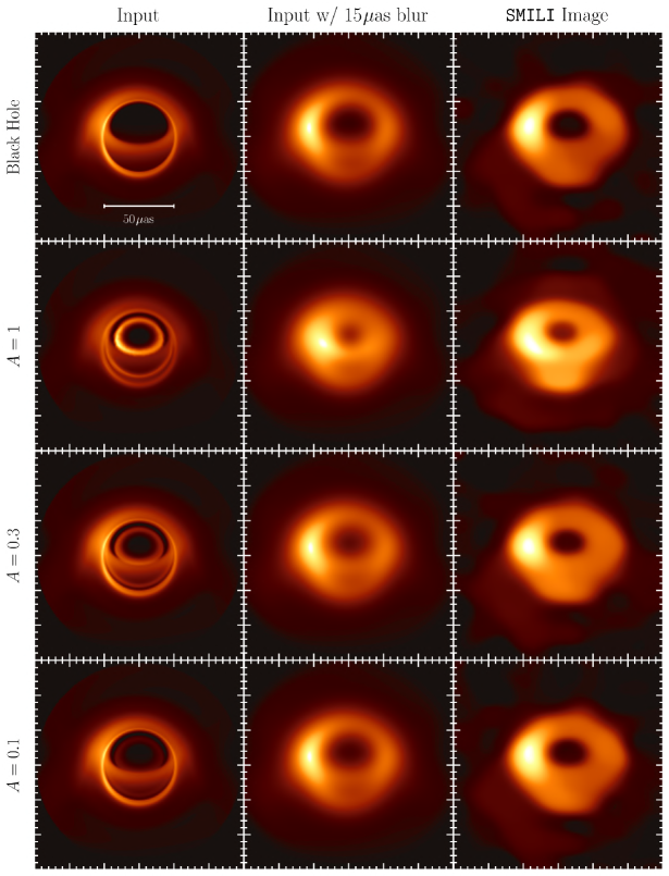
4.2.2 Constraints from EHT Images

Figures 13, 14 and 17 in Paper III show a range of images of Sgr A^∗ obtained by applying different image reconstruction techniques to the EHT 2017 data. The vast majority of images show a ring-like morphology with a pronounced dark shadow region at the center. These images are visibly different from the synthetic blurred image shown in the second row middle panel in our Figure 15. We can thus exclude this particular model using EHT observations.

The right four panels in Figure 15 show image reconstructions of the four synthetic models shown in the left panels using one of the image reconstruction methods described in Paper III. For each model, synthetic visibility data were generated with the same $(u,v)$-coverage as in the April 7 EHT observations of Sgr A^∗, and the appropriate amount of noise was added to match the noise present in the real data. These synthetic visibilities were then analysed using the SMILI top set (see Paper III for details) and the resulting images are shown in the panels on the right in Figure 15. The SMILI reconstructions are fairly similar to the $15\,\mu$as-blurred images shown in the corresponding central panels, though the SMILI images appear to be slightly more blurred. More interestingly, the SMILI image of the $A=1$ reflecting surface model (second row right panel) is quite different from the reconstruction of the black hole model (top row right panel). This confirms our expectation that a surface which reflects in-falling radiation with 100% efficiency can potentially be ruled out by EHT 2017 observations of Sgr A^∗ (modulo the many caveats mentioned in Section 4.2.1). In the case of the $A=0.3$ model, and especially the $A=0.1$ model, the SMILI reconstructions do not differ much from the black hole image, hence it would be hard to distinguish such models using the current EHT data.

Another way of comparing models is to measure the brightness depression in the shadow region of the image. For instance, Table 13 in Paper III presents estimates of a parameter $f_{c}$, which measures the ratio of the brightness at the center of the ring image to the mean brightness around the ring. This quantity is a measure of the brightness depression in the central shadow region of the image. From Figure 22 in Paper III, the estimate based on SMILI is $f_{c}\approx 0.2$, with not much probability that $f_{c}>0.3$. This implies that the image intensity in the shadow region in Sgr A^∗ is very likely $<30\%$ of the mean intensity around the ring.

Such a degree of flux depression is inconsistent with the blurred synthetic image and SMILI reconstructed image in the second row of Figure 15. That particular model could be potentially ruled out. However, the dynamic range of images based on the current EHT 2017 data is too low, and its angular resolution is too poor, to constrain a weakly reflecting surface in Sgr A^∗, such as the models in the third and fourth rows of Figure  15.

An array with more stations and with larger bandwidth (e.g., the proposed Next Generation Event Horizon Telescope, Doeleman et al. 2019; Raymond et al. 2021) would solve the sensitivity problem. However, to improve the angular resolution substantially, it will be necessary to expand the telescope array into space by sending one or more radio dishes into large-radius orbits around the Earth (Palumbo et al., 2019; Roelofs et al., 2020b; Fish et al., 2020; Gurvits et al., 2021; Kudriashov et al., 2021; Fromm et al., 2021). With such an expanded array, we might be able to observe images with sufficient angular resolution to see some of the details revealed in the various panels in the left column of Figure 15 and to check for the presence of a surface in Sgr A^∗. Furthermore, if a surface is present, we might be able to determine the albedo and the surface radius.

Chael et al. (2021) show that, with better sensitivity and angular resolution than the present EHT is able to provide, the observed image of a hot accretion flow around a supermassive black hole could be used to delineate the inner edge of the accretion disk. Their interest is to use this technique to identify the edge of the event horizon. However, their method could equally well be used to measure the radius of a potential surface. This might provide a direct estimate of $R_{*}$.

Additionally, it may be possible to observe time-delayed echoes from a reflecting surface. In the case of time-variable emission from the accretion flow, e.g., sub-millimeter or infrared flares, the observer would see both the primary signal from the emitting gas element as well as a delayed reflected copy of the same radiation. This is the electromagnetic analog of gravitational wave echoes that have been searched for in LIGO/Virgo observations of merging stellar-mass black holes (Abedi et al., 2017; Westerweck et al., 2018). However, here it could be done with spatially resolved images, with all the rich detail they can provide. We do not pursue electromagnetic echoes further, but note that their presence could potentially be explored already using existing image-integrated light curve data.

4.3 Surfaceless Horizonless Compact Objects

As examples of horizonless compact objects without surfaces, we consider black-hole mimickers such as (mini) boson stars, for which synthetic images from covariant MHD simulations of radiatively inefficient accretion flows have recently been obtained in Olivares et al. (2020). It was shown there that a region with a central brightness depression could appear in the final observed image of an unstable boson star (model A there), despite the absence of an unstable photon orbit in that spacetime. These features are the result of an effective low-density region that appears in the center of the spacetime due to a centrifugal barrier. The unstable boson star has a significantly smaller intrinsic source size than corresponding constraints of Sgr A^∗ thereby ruling it out as a candidate alternative. Similarly, for the stable boson star configuration considered in Olivares et al. (2020), there is a complete absence of a central brightness depression with the inner image being extremely bright, akin to a radiating surface (see, e.g., Fromm et al., 2021). Given the EHT constraints a mini boson star becomes an unlikely candidate as a black hole mimicker to describe Sgr A^∗, since their image morphologies are generally too compact and lack both a characteristic ring-like feature and a central brightness depression. However a more extensive study of a boson star spin, compactness and astrophysical setup should be considered to make this argument conclusive (e.g., Vincent et al. 2021).

While the size of the bright emission ring/central brightness depression will be necessary to rule out or constrain the black hole and non-black hole models considered in Section 5 below, the very presence of a central brightness depression in the 2017 image of Sgr A^∗ (see; , and Paper V) is sufficient to rule out various models for compact objects that do not possess photon spheres. For example, these observations rule out the possibility that Sgr A^∗ is a nonspinning Joshi-Malafarina-Narayan-2 (Joshi et al. 2014; JMN-2) naked singularity since these exotic compact objects do not cast shadows (Shaikh et al., 2019). We note that the JMN-2 spacetime is an exact solution of the Tolman-Oppenheimer-Volkoff equations of General Relativity, can form as the nonempty end-state of the gravitational collapse of a (non-thermal) perfect fluid from regular Cauchy data, and photons in the spacetime move on null geodesics of the metric tensor (see also the associated discussion in Section 5.2). We assume the naked singularity present at $r=0$ does not interact with matter or radiation (classical gravity).

5 Metric tests from shadow size

In Section 3.5, we used the prior information on the mass-to-distance ratio of the Sgr A^∗ black hole to calculate the predicted size of its shadow and compared the result to the size inferred from the EHT images and visibility-domain model fitting. We based this prediction on the Kerr metric and found that there is no evidence for any violations of the theory of General Relativity. Our goal in this section is to use these bounds on plausible deviations in the shadow size that are still consistent with the imaging data in order to place constraints on deviations of the parameters of the underlying black-hole metric.

We will follow two complementary approaches. First, in Section 5.1, we will constrain the parameters of stationary metrics that are agnostic to the underlying physical theory. These have been designed in a way that they reduce to the Kerr metric, when the deviation parameters are set to zero, but remain free of pathologies for a wide range of parameter values (Psaltis et al., 2020a). Although these metrics do not arise from any particular modification to gravity, they allow us to explore phenomenologically a very broad range of possibilities, which can be mapped afterwards to parameters of a fundamental theory. Second, in Section 5.2, we will constrain the parameters of stationary metrics that are generated by various matter distributions and/or those that arise from specific modifications to the theory of gravity, and which depend on additional generalized charges (Kocherlakota et al., 2021). Although the latter represent only particular types of deviations from General Relativity, they allow us to translate directly the constraints from the EHT images to bounds on physical parameters. Finally, in Section 5.3, we will compare the constraints on the various metrics in terms of their asymptotic post-Newtonian parameters in order to demonstrate that, fundamentally, the bounds imposed by the EHT imaging observations of Sgr A^∗ depend weakly on the particular metrics used to describe deviations from Kerr.

Figure 16: Numerical constraints on various deviation parameters for the JP and MGBK metrics as a function of the dimensionless black-hole spin placed by the requirement that the predicted size of the black-hole shadow is consistent with the size inferred for Sgr A^∗. Here the shading shows the regions of the parameter space that are ruled out by the bound derived from the calibration based on the Keck mass measurement, the eht-imaging algorithm, and the GRMHD simulation library, as an example. The left (right) panels show constraints for the JP (MGBK) metrics, while the different symbols/colors in the top and bottom panels show the effect of the secondary deviation parameter and the inclination of the observer, respectively. In the top panels we set the inclination angle to $i=42^{\circ}$ and set the secondary deviation parameter to zero in the bottom panels. In all panels the black dashed lines correspond to the analytic constraints for non-spinning black holes. The non-monotonic behavior of the constraints are due to the fact that both the size and the shape of the shadows are affected by the deviation parameters. The measurement of the shadow size constrains primarily the parameters that quantify deviations in the $tt-$components of the various metrics, as expressed in areal coordinates, and the resulting bounds depend only weakly on black-hole spin or observer inclination.

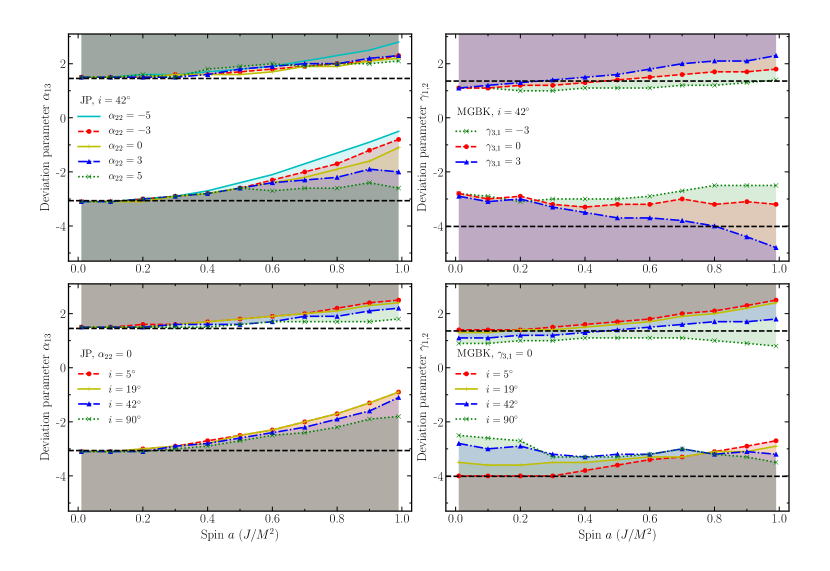
Throughout this section, for clarity of presentation, we will use the bounds $\delta=-0.04^{+0.09}_{-0.10}$ (Keck) and $\delta=-0.08^{+0.09}_{-0.09}$ (VLTI) on the fractional deviation inferred from the predicted shadow size, as calculated for the fiducial analyses that use the Keck and VLTI priors on the mass-to-distance ratio, the eht-imaging imaging method, and the GRMHD library for quantifying the theoretical uncertainties. Where it is not possible to show both bounds, we will show the Keck bound as an example. This constraint depends weakly on the choice of priors and techniques. In particular, the fiducial bounds correspond to the following constraints on shadow size:

$$\begin{split}3\sqrt{3}(1-0.14)M&\lesssim\tilde{r}_{\text{sh}}\lesssim 3\sqrt{3}(1+0.05)M,\\ 4.5M&\lesssim\tilde{r}_{\text{sh}}\lesssim 5.5M,\end{split}$$ (12)

for Keck and

$$\begin{split}3\sqrt{3}(1-0.17)M&\lesssim\tilde{r}_{\text{sh}}\lesssim 3\sqrt{3}(1+0.01)M,\\ 4.3M&\lesssim\tilde{r}_{\text{sh}}\lesssim 5.3M,\end{split}$$ (13)

for VLTI, where we have set $G=c=1$, as we will do throughout this section. For the different metrics employed in this section, we calculate the fractional diameter deviation of the metric as the relative difference between the analytic shadow diameter and the Schwarzschild diameter, namely:

$$\delta_{\rm metric}=\frac{\tilde{d}_{\mathrm{metric}}}{6\sqrt{3}}-1\,,$$ (14)

where $\tilde{d}_{\rm metric}$ is the median shadow diameter, i.e., the locus of critical impact parameters.

Throughout this section we will not consider constraints on the circularity of the shadow. This is due to the sparse interferometric coverage of 2017 observations, which may lead to significant uncertainties in circularity measurements that we do not quantify here. In addition to measurement uncertainty, we also do not quantify the theoretical uncertainty between the circularity of the shadow and that of the observational feature. However, in future EHT observations with additional telescopes the circularity of the shadow may potentially be used for constraints on deviations from the Kerr metric.

5.1 Constraints on Metrics with Parametric Deviations

According to the no-hair theorem in General Relativity, the only stationary, asymptotically flat, Ricci-flat spacetime that is free of pathologies is the one described by the Kerr metric. We do not consider here the astrophysically irrelevant case of black holes with a net electric charge (c.f. Section 5.2). As a result, introducing simple phenomenological deviations to the Kerr metric leads to pathologies that severely constrain our ability to make predictions for the size of the black-hole shadow, especially in the case of spinning black holes (see Johannsen 2013b for a detailed study of the pathologies of several parametrized metrics and Kocherlakota & Rezzolla 2022 for an analysis of theoretically-allowed parameter spaces of the RZ metric). For this reason, several parametrized metrics have been developed in the last decade that allow for general deviations from the Kerr metric while minimizing pathologies mostly by relaxing the assumption of Ricci flatness. These parametrized metrics are completely agnostic to an underlying physical theory and, therefore, significant assumptions must be made for stability tests (see e.g., Suvorov & Völkel 2021 for a quasi-normal-mode analysis of the RZ metric). Among these metrics, we choose three representative ones: the so-called JP metric (Johannsen & Psaltis 2011, which was further developed to ensure the presence of a Carter-like integral of motion in Johannsen 2013a); the Modified Gravity Bumpy Kerr (MGBK) metric (Vigeland et al., 2011); and the so-called RZ metric (Rezzolla & Zhidenko 2014, which was further developed to include the effects of spin in Konoplya et al. 2016). We will derive analytic constraints for all three metrics and will use numerical calculations to derive spin-dependent constraints for both the JP and MGBK metrics.

Earlier studies have demonstrated that, because of a near cancellation between the effects of frame dragging and of the quadrupole moment of the spacetime, the spin of the black hole affects the shadow size only marginally (see, e.g., Johannsen & Psaltis 2010; Psaltis et al. 2020a). Therefore, the bounds on the deviation parameters imposed by the measurement of the black-hole shadow in Sgr A^∗ are also expected to depend weakly on black-hole spin. We demonstrate this in Figure 16, which shows the limits on different deviation parameters of the JP and MGBK metrics as a function of black-hole spin, for various observer inclinations, and for different values of the secondary deviation parameters. The horizontal dashed curves show the bounds for non-spinning black holes when the secondary deviation parameters are zero. For this figure, we have set the parameters that affect the $g_{tt}$–component of the metric at the $r^{-2}$ order to zero (i.e., $\alpha_{12}=0$ and $\gamma_{4,2}=-\frac{1}{2}\gamma_{1,2}$, see also Section 5.2) so we can focus on higher order effects. The resulting constraints are of order-unity and weakly dependent on spin, inclination angle, and the values of secondary deviation parameters.

The simulations used for this figure are described in Medeiros et al. (2020). In these simulations we assume that the geodesic equation holds for all metrics and solve for the trajectories of photons ignoring matter effects. We define the boundary of the black hole shadow as the critical impact parameter between photon trajectories that fall into the event horizon and those that escape to infinity. As was done in Section 3 we define the size of a shadow as its median radius and compare this measurement to the bounds on shadow size from the eht-imaging algorithm, the GRMHD simulation library, and the prior mass and distance measurements from Keck.

As found in Psaltis et al. (2020a), the measurement of the size of the black-hole shadow places constraints of order unity primarily on parameters such as $\alpha_{13}$ and $\gamma_{1,2}$ that depend weakly on the magnitude of the black-hole spin. What is common between these parameters is that they describe deviations in the $tt-$component of the black-hole metric, as expressed in areal coordinates.

Since spin has a relatively small effect on the predicted shadow size and, hence, on the metric constraints, we now focus on a more detailed exploration of the constraints on these three metrics when we set the spin to zero (i.e., in the limit of spherical symmetry). The radius of the shadow in this limit is given by (Psaltis et al., 2020a)

$$r_{\mathrm{sh}}=\ \frac{r_{\mathrm{ph}}}{\sqrt{-g_{tt}(r_{\mathrm{ph}})}},$$ (15)

where

$$r_{\mathrm{ph}}\equiv 2g_{tt}(r_{\mathrm{ph}})\left(\left.\frac{dg_{tt}}{dr}\right|_{r_{\mathrm{ph}}}\right)^{-1}\;,$$ (16)

is the radius of the photon orbit.

For non-spinning black holes, the $tt-$component of the JP metric in areal coordinates is (see Johannsen 2013b)

$$g_{tt}^{\mathrm{JP}}=-\left(1-\frac{2}{r_{A}}\right)\left(1+\sum^{\infty}_{i=2}\frac{\alpha_{1i}}{r_{A}^{i}}\right)^{-2}$$ (17)

where $\alpha_{1i}$ are deviation parameters and the subscript $A$ denotes the fact that we use areal coordinates.

Figure 17: Analytic constraints on deviation parameters for the JP, MGBK, and RZ metrics. The regions excluded by the Sgr A^∗ constraints using Keck (VLTI) are shown in blue (magenta), see also Equations 12 and 13. For each curve we allow only one parameter to vary while setting the others to zero. The original $g_{tt}$ components of the metrics were used for this plot, not their expansions.

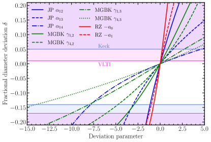
The $tt-$component of the non-spinning MGBK metric in areal coordinates is (see Vigeland et al. 2011; Gair & Yunes 2011)

$$g_{tt}^{\mathrm{MGBK}}=-\left(1-\frac{2}{r_{A}}\right)\left[1-\gamma_{1}(r_{A})-2\gamma_{4}(r_{A})\left(1-\frac{2}{r_{A}}\right)\right]$$ (18)

where $\gamma_{1}(r_{A})$ and $\gamma_{4}(r_{A})$ are defined by

$$\gamma_{A}=\sum^{\infty}_{n=2}\frac{\gamma_{A,n}}{r_{A}^{n}},$$ (19)

$A=1$ or 4, and $\gamma_{A,n}$ are the deviation parameters.

Finally, the $tt-$component of the spherically symmetric RZ metric in areal coordinates is (see Rezzolla & Zhidenko 2014)

$$g_{tt}^{\mathrm{RZ}}=-x\left[1-\epsilon(1-x)+(a_{0}-\epsilon)(1-x)^{2}+\tilde{A}(x)(1-x)^{3}\right]$$ (20)

where

$$\begin{split}x&\equiv 1-\frac{r_{0}}{r_{A}},\\ \tilde{A}(x)&=\frac{a_{1}}{1+\frac{a_{2}x}{1+\frac{a_{3}x}{...}}},\end{split}$$ (21)

and $r_{0}$ is the coordinate radius of the infinite redshift surface (identified with the horizon if no pathologies exist). The parameters $\epsilon,\,a_{1},\,a_{2},\,...$ are the deviation parameters. As done in Psaltis et al. (2021), we write all radii in terms of the mass of the black hole at infinity which fixes one of the parameters

$$\epsilon=-\left(1-\frac{2}{r_{0}}\right).$$ (22)

For simplicity we assume $r_{0}=2$ throughout the rest of this section.

Using these analytic expressions, we calculate the size of the black-hole shadow as a function of the various deviation parameters using equation (15). We then apply the bounds on the shadow size imposed by the Sgr A^∗ images and obtain constraints on the deviation parameters of the various metrics. The dashed lines in Figure 16 compare the analytic bounds with those obtained numerically for the spinning spacetimes.

Because we use only one measured quantity from the EHT image of Sgr A^∗, i.e., the size of the black-hole shadow, but the $tt-$components of each metric depend on a series of deviation parameters, it follows that the EHT observations place, in fact, correlated constraints on these parameters. These can be thought of as subspaces in the multidimensional parameter space of deviations and are very difficult to visualize in full generality. In Figure 16, we showed one particular cross section of this parameter space in which the various parameters were combined such that deviations from Kerr appear only at the second or higher post-Newtonian order.

Figure 17 shows a different cross section of these constraints, where we have varied only one parameter at a time, setting all others equal to zero. The constraints derived from the Keck bounds are also summarized in Table 3. The deviation parameters that correspond to higher-order corrections (as denoted by the second integer in their subscripts) affect the size of the shadow less strongly that the lower-order parameters and are, therefore, less constrained. We will return to the magnitudes of these constraints in Section 5.3, after we discuss the bounds on metrics that correspond to solutions of particular modified gravity theories.

Table 3: Constraints on Deviation Parameters of Various Metrics

Parametrized metric	Constraints
JP	$\begin{array}[]{lcl}-1.1\lesssim&\alpha_{12}\lesssim 0.5\\ -3.1\lesssim&\alpha_{13}\lesssim 1.5\\ -7.8\lesssim&\alpha_{14}\lesssim 4.6\\ \end{array}$
MGBK	$\begin{array}[]{lcl}-4.0&\lesssim\gamma_{1,2}\lesssim 1.4\\ -4.8&\lesssim\gamma_{4,2}\lesssim 1.3\\ -8.0&\lesssim\gamma_{1,3}\lesssim 2.7\\ -14.0&\lesssim\gamma_{4,3}\lesssim 3.8\end{array}$
RZ	$\begin{array}[]{lcl}-0.2\lesssim&a_{0}\lesssim 0.7\\ -0.3\lesssim&a_{1}\lesssim 1.0\\ \end{array}$

• Notes: Here and in Table 4 we use the bound derived from the calibration based on the Keck mass measurement, the eht-imaging algorithm, and the GRMHD simulation library, as an example.

• JP, MGBK, and RZ are parametrized metrics that deviate from Kerr (see Johannsen & Psaltis 2011; Vigeland et al. 2011; Rezzolla & Zhidenko 2014 for details on these metrics).

Figure 18: The dependence of the fractional shadow diameter deviation from the Schwarzschild value (left) on the relevant physical “charges” of various nonspinning black hole metrics and (right) on the black-hole spins, for fixed values of the charges and for an observer inclination $i=\pi/2$. The white regions correspond to shadow sizes that are consistent at the 68% level with the 2017 EHT observations for Sgr A^∗. As in the case of the Kerr and of the parametric metrics, the spin of the black hole introduces only minor corrections to the predicted shadow size and, hence, to the metric constraints. Current EHT imaging observations of Sgr A^∗ are inconsistent with some metrics when their physical charges are comparable to their maximum theoretically-allowed values. We use the median shadow diameter to characterize the size of the noncircular shadows cast by the spinning black holes (right), as done in Section 3.

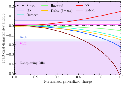
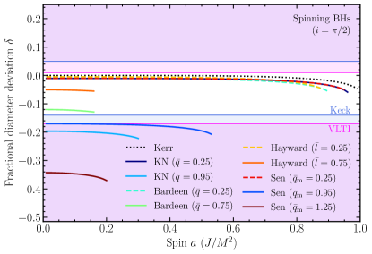
5.2 Constraints on Specific Compact Object Spacetime Metrics

Detecting possible deviations from the Kerr metric using the agnostic approach discussed above can be used to infer constraints on multiple asymptotic expansion coefficients of the spacetime, test the no-hair theorem, assess the Ricci-flatness of black-hole metrics, etc. In this Section, we follow a complementary approach to determining whether specific fundamental principles of the theory of gravity are violated by considering explicitly theories that incorporate such violations by design, finding (stationary) solutions to the associated field equations that describe supermassive compact objects such as Sgr A^∗, and determining whether their images, when undergoing similar accretion processes, are compatible with those observed with the EHT.

Adopting this approach helps us assess the necessity of including additional fundamental fields (such as dilatons or axions) in the description of the classical theory and yield quantitative constraints on the amount of build-up of various fields in the vicinity of supermassive compact objects (see, e.g., Kocherlakota et al. 2021). This could be instructive of the astrophysical processes that may have produced them. Studying the images of available solutions allows us also to address questions related to the type of object that Sgr A^∗ is, e.g., whether it is a naked singularity, a boson star, or a black hole. Finally, working with a specific theory enables a comparison of its predictions for a variety of other physical scenarios with already existing or future observations, for its overall compatibility, as discussed in Section 6.

Alternative Black Holes.—As an example, the equivalence principle is a fundamental building block of the theory of gravity and has thus far been tested in various regimes by complementary experiments. It comprises three aspects (Dicke, 2019; Will, 2014): the weak equivalence principle (WEP), local Lorentz invariance (LLI), and local positional invariance (LPI). To demonstrate the scope of testing theories that violate the WEP and LPI with the EHT, we will consider here black-hole solutions from two Einstein-Maxwell-dilaton-axion (EMda) theories (Gibbons & Maeda 1988; Garfinkle et al. 1991; Sen 1992; García et al. 1995; Kallosh et al. 1992; see also the discussion in, e.g., Magueijo 2003 and Kocherlakota & Rezzolla 2020), which emerge as the low-energy effective descriptions of the heterotic string. This conservative choice allows us to be certain that (a) the form of the equations that describe the dynamics of accreting plasma flow around EMda black holes is identical to those in General Relativity due to the minimal coupling of matter to Einstein-Hilbert gravity via the metric tensor, and (b) photons move on null geodesics of the metric tensor since electromagnetism is described by the (linear) Maxwell Lagrangian (see, e.g., Sec. 4.3 of Wald 1984).

Synthetic images of radiative inefficient accretion flows onto Gibbons-Maeda-Garfinkle-Horowitz-Strominger black holes (Gibbons & Maeda, 1988; Garfinkle et al., 1991), which describe charged, static black holes in one of the EMda theories (henceforth the EMd-1 for brevity), have been constructed in Mizuno et al. (2018), using MHD simulations (see also Figure 6). It was demonstrated there that the final images of these EMd-1 black holes are comparable to those of the Schwarzschild/Kerr black holes. More recently, properties of images of (Kerr-)Sen black holes (Sen, 1992), which are the spinning generalizations of the EMd-1 black holes, have been calculated and characterized in Younsi et al. (2021), when undergoing accretion that is described by the semi-analytic model of Özel et al. (2021) (see also Figure 6). To compare the features of Sen black holes against their general relativistic counterparts, we consider the Reissner-Nordstrom (RN; Reissner 1916; Nordström 1918) and the Kerr-Newman (KN; Newman et al. 1965) solutions, which describe charged black holes with and without spin respectively.

We also consider solutions arising from various attempts to regularize the central singularities of classical black holes within General Relativity. In particular, we consider solutions by Bardeen (1968), Hayward (2006), and Frolov (2016). Such solutions are typically nonempty and the matter present, in a stationary configuration, typically violates one or more energy conditions (Hawking & Ellis 1973; Curiel 2017). Studying the images of available solutions that can be used to model compact objects allows us to test for possible violations of components of the equivalence principle or of energy conditions. We also include here the static Kazakov & Solodukhin (1994) (KS) solution which attempts to smear out the central singularity onto a surface. Additionally, we also consider the spinning counterparts of the Bardeen and Hayward metrics (Abdujabbarov et al., 2016). To conduct the analysis below, we have implicitly assumed that the “ordinary” matter in the accretion flow does not interact with the background matter in the nonempty spacetimes we consider here.

Figure 19: We show here the constraints on two EMda solutions from different EMda theories. In the top plot we show the constraints on the parameter space of a nonspinning black hole from an EMda theory with two $U(1)$ gauge fields (Kallosh et al., 1992) whereas in the bottom plot we show the constraints on the parameter space of a spinning Sen black hole from an EMda theory with a single $U(1)$ gauge field (Sen, 1992).

Figure 20: Same as Figure 18 but for metrics that describe various naked singularities (denoted by a star) and a wormhole.

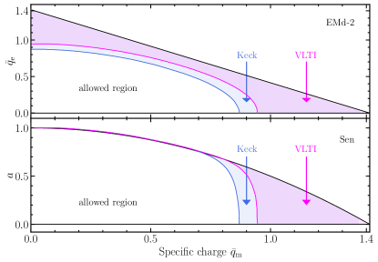
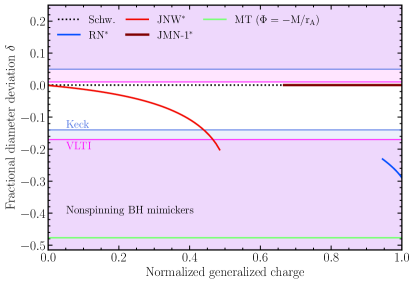
Figure 18 shows the dependence of the deviation of the shadow size from the Schwarzschild prediction on the parameters (the “generalized charges” or simply charges henceforth) of the various metrics discussed above (see also Section IV of Kocherlakota & Rezzolla 2020 for further details). In this figure, each relevant physical parameter has been normalized to its maximum theoretically-allowed value (see also Table 5). Similarly to the case of the Kerr and of the parametric metrics, we find that the black-hole spin introduces minor corrections to the size of the shadow, which allows us to focus on nonspinning spacetimes. Moreover, the current bounds imposed by the EHT images of Sgr A^∗ place constraints of order unity to the charges of several of the spacetimes, which are comparable to their maximum values, by construction. Figure 19 focuses on the constraints that we can set on the relevant parameter spaces of all the black holes from the two EMda theories considered here: the top panel shows the charged, nonspinning “EMd-2” solution from one theory (Kallosh et al., 1992). From the other theory, we show in the bottom panel the parameter space for the spinning Sen black hole (Sen, 1992) (the EMd-1 black hole corresponds to the $a=0$ line). As can be seen from these figures, we find no evidence of violations of the equivalence principle or of the presence of energy-conditions violating matter within the present context.

Thus far we have considered in detail the possibility that Sgr A^∗ is a supermassive black hole (described by different metrics) as well as the alternative that it possesses a material surface (Section 4). We have also considered the possibility that Sgr A^∗ is a surfaceless horizonless compact object without a photon sphere, with focus on mini-boson stars and naked singularities, in Section 4.3. Here, using specific solutions, we will address whether the spacetime in its vicinity can be well modeled by that of a naked singularity with a photon sphere, and, later on, by a wormhole. Since all of the naked singularity solutions we consider here arise from metric theories of gravity with the electromagnetic sector being governed by the linear Maxwell Lagrangian, photons move on null geodesics of the metric tensor, as discussed above. Since we consider exact solutions to the classical theory, we assume that the background spacetimes are static and that the naked singularities at $r=0$ do not interact with matter or radiation in any way.

Naked Singularities.—For an example of a naked singularity spacetime, we will consider the Reissner-Nordström metric (Reissner, 1916; Nordström, 1918), characterized by specific electromagnetic charges of $\bar{q}>1$, and denote it by RN^∗. These spacetimes admit photon spheres only for $1<\bar{q}\leq\sqrt{9/8}$, and Figure 20 shows only this range, normalized to the maximum. The Janis-Newman-Winicour (JNW; Janis et al. 1968) naked singularity spacetime is a solution of the Einstein-Maxwell-scalar theory with a theoretically-allowed scalar charge parameter range of $0<\hat{\bar{\nu}}<1$. However, the JNW naked singularities only cast shadows when $0<\hat{\bar{\nu}}\leq 0.5$, as indicated in Figure 20. We will also consider a new class of naked singularities within General Relativity, namely the Joshi-Malafarina-Narayan-1 (JMN-1; Joshi et al. 2011) naked singularities. This class of solutions describes a one-parameter $M_{0}$ family of static spacetimes containing a compact region $r_{A}<r_{A,\text{b}}\equiv 2M/M_{0}$ filled by an anisotropic fluid, where $M$ is the ADM mass of the spacetime. This spacetime can be attained at asymptotically late times as a result of gravitational collapse from regular initial data (Joshi et al. 2011; see also Section IV of Dey et al. 2019) and contains a photon sphere when $r_{A,\text{b}}<3M$ or equivalently when $M_{0}\geq 2/3$ contributed by the exterior Schwarzschild spacetime.

Spherical Bondi-Michel accretion onto JMN-1 naked singularities has been studied in Shaikh et al. (2019), where it was found that the final images of JMN-1 naked singularities with photon spheres are indistinguishable from those of a Schwarzschild black hole. More strikingly, for the same approximate luminosity as Sgr A^∗ at 200 GHz, accretion flows onto these singularities have spectra nearly identical to that of a Schwarzschild black hole (see Fig. 6 therein), indicating that a JMN-1 naked singularity with a photon sphere may be one of the best possible black-hole mimickers for Sgr A^∗ (cf. Section 4).

Figure 20 shows the bounds imposed by the EHT images of Sgr A^∗ on the the physical charges of these metrics that describe naked singularities. With the exception of the Reissner-Nordström metric, which predicts shadow sizes that are significantly smaller than what is observed, the possibility that Sgr A^∗ is a naked singularity cannot be ruled out based on the metric tests we describe in this section.

Wormholes.—As an example of a wormhole, we consider nonspinning, traversible Morris-Thorne (MT) metrics (Morris & Thorne, 1988) in General Relativity, for which the $tt$-components of the metric are determined by the “redshift function” $\Phi$ as $g_{tt}=-\exp{(2\Phi)}$. For wormholes in General Relativity to be traversible, the spacetime must necessarily contain energy-condition-violating matter and lack event horizons. The location(s) of the circular null geodesic(s) in this spacetime can be obtained by solving $-1+r_{A}~{}d\Phi/dr_{A}=0$. If we restrict to the simplest case of an MT wormhole with a single unstable circular null geodesic, which can then be identified as the location of the photon sphere, e.g., by setting $\Phi=-r_{A,\text{t}}/r_{A}$ as in Bambi (2013), we find that the (Keplerian/ADM) mass definition forces $r_{A,\text{t}}=M$. This implies a shadow radius of $r_{\text{sh}}=e~{}M\approx 2.72~{}M$ or equivalently $\delta\approx-0.48$, which is immediately ruled out by the present considerations (see Figure 20).

Finally, as noted above in Section 4, improved angular resolution with space-VLBI would greatly help constrain possible metric-deviations from the Kerr geometry. Notably, it would be possible to infer the spin of Sgr A^∗, when modelled as a Kerr black hole, if we are able to achieve a precision of $|\delta|<0.07$ (Johannsen & Psaltis 2010; see also Fig. 18). Shadows of spinning MT wormholes (Teo, 1998) have recently been considered in Shaikh (2018), where it was shown that their shape can vary considerably from that of a Kerr black hole, and possibly be detected with future EHT or ngEHT measurements. Spacetimes admitting multiple circular null geodesics were considered by Wielgus et al. (2020), an example of which is given by black holes in a non-minimal Einstein-Maxwell-scalar theory (Gan et al., 2021). Presence of a persistent multi-ring structure in an EHT image would constitute a robust topological discriminant of this family of spacetimes, particularly with future observations at higher resolution and flux-sensitivity.

Table 4: Post-Newtonian Coefficients of Parametrized Metrics

Parametrized metric	$\kappa_{1}$	$\kappa_{2}$	Constraints
JP	$-\alpha_{12}$	$-2\alpha_{12}+\alpha_{13}$	$\begin{array}[]{lcl}-0.3&\lesssim\kappa_{1}\lesssim 0.7\\ -3.1&\lesssim\kappa_{2}\lesssim 1.5\\ \end{array}$
MGBK	$-\frac{1}{2}\gamma_{1,2}-\gamma_{4,2}$	$-\gamma_{1,2}+\frac{1}{2}\gamma_{1,3}-4\gamma_{4,2}+\gamma_{4,3}$	$\begin{array}[]{lcl}-0.3&\lesssim\kappa_{1}\lesssim 0.9\\ -4.0&\lesssim\kappa_{2}\lesssim 1.3\\ \end{array}$
RZ	$2a_{0}$	$4\left(a_{0}-\frac{a_{1}}{1+\frac{a_{2}}{1+\frac{a_{3}}{...}}}\right)$	$\begin{array}[]{lcl}-0.3&\lesssim\kappa_{1}\lesssim 0.9\\ -4.0&\lesssim\kappa_{2}\lesssim 1.3\\ \end{array}$

Table 5: Post-Newtonian Coefficients of Specific Compact Object Spacetime Metrics

Spacetime	Charge Range	Constraints	$\kappa_{1}$	$\kappa_{2}$
RN	$0<\bar{q}\leq 1$	$0<\bar{q}\leq 0.84$	$\bar{q}^{2}/2$	$0$
RN*	$1<\bar{q}$	$\times$	$\bar{q}^{2}/2$	$0$
Schwarzschild	$-$	$-$	$0$	$0$
Bardeen	$0<\bar{q}<\sqrt{16/27}$	$-$	$0$	$-3\bar{q}^{2}/2$
Frolov	$0<\bar{l}<\sqrt{16/27},0<\bar{q}\leq 1$	see, e.g., Figure 18	$\bar{q}^{2}/2$	0
Hayward	$0<\bar{l}<\sqrt{16/27}$	$-$	$0$	$0$
MT Wormhole	$-$	$\times$	$-1$	$-2/3$
KS	$0<\bar{\alpha}$	$0<\bar{\alpha}\leq 0.79$	$-\bar{\alpha}^{2}/4$	$0$
EMd-1†	$0<\bar{q}<\sqrt{2}$	$0<\bar{q}<0.87$	$\bar{q}^{2}/2$	$\bar{q}^{4}/8$
EMd-2†	$0<\bar{q}_{\text{e}}\leq\sqrt{2}-\bar{q}_{\text{m}}<\sqrt{2}$	Figure 19 (top)	$\left(\bar{q}_{\text{m}}^{2}+\bar{q}_{\text{e}}^{2}\right)/2$	$\left(\bar{q}_{\text{m}}^{2}-\bar{q}_{\text{e}}^{2}\right)^{2}/8$

• Notes: We denote by crosses and dashes spacetimes that are entirely ruled out and that are unaffected by the EHT measurements.

5.3 Comparisons Between Metric Constraints

In the discussion above, we used the inferred size of the black-hole shadow in Sgr A^∗ in order to place constraints on parameters of metrics that deviate from Kerr. For the metrics that are solutions to particular modifications to General Relativity, these parameters (or “charges”) correspond to particular properties of the theory or of the back hole itself. For the parametrized metrics, these parameters are phenomenological coefficients that are agnostic to any particular aspect of the underlying theory. Even though it might appear that these bounds are specific to the particular metric used, we will show here that they describe deviations from Kerr that are mathematically very similar to each other and nearly independent of the characteristics of the metric used.

First, as Figures 16 and 18 show, the constraints imposed by the measurement of the size of a black-hole shadow depend weakly on the spin of the black hole, for all the metrics explored. As discussed in Section 5.1, for metrics with zero spin, it can be shown analytically that the measurements lead to constraints only on the parameters that enter the $tt-$component of the metric in areal coordinates. The consequence of these two statements is that, for all spins, the primary constraints imposed by the measurement of a shadow size will be only on one of the metric components, largely independent of the other metric details.

Figure 21: Constraints on the post-Newtonian coefficients $\kappa_{1}$ (top panel) and $\kappa_{2}$ (bottom panel) of the Sgr A^∗ metric imposed by the EHT images. We include three parametrized metrics as well as several metrics that are known solutions to particular modified gravity theories. For each curve, we only allow one of the first two post-Newtonian coefficient to vary and set the others to zero. The bounds on the post-Newtonian coefficients depend weakly on the specific properties of the metric used to obtain them.

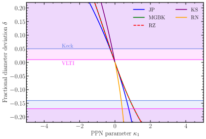
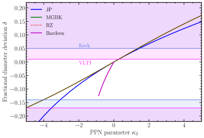
Translating directly the bounds on the parameters of one metric to those of another is non-trivial because of the usual coordinate and gauge ambiguities that are inherent to relativistic spacetimes. However, one avenue of making this comparison is by exploring the asymptotic behavior of these metrics towards radial infinity. In particular, we write the $tt-$component in areal coordinates in terms of the parametrized post-Newtonian (PPN) expansion

$$g_{tt}=-1+\frac{2}{r_{A}}-2\left(\frac{\kappa_{1}}{r_{A}^{2}}\right)+2\left(\frac{\kappa_{2}}{r_{A}^{3}}\right)-2\left(\frac{\kappa_{3}}{r_{A}^{4}}\right)+\mathcal{O}(r_{A}^{-5})$$ (23)

and connect without ambiguity the post-Newtonian coefficients of each metric to each particular parameter. We then translate the bounds of the parameters to constraints on these post-Newtonian coefficients and compare the results obtained with different metrics.

We emphasize that we do not use these post-Newtonian expansions in order to calculate black-hole shadows, which would have been inappropriate given that the size of the shadow is comparable to the horizon radius. Instead, we calculate shadow sizes and place constraints on the particular parameters of each of the metrics that has been developed specifically for use in the strong-field regime. We only use the post-Newtonian coefficients as a mechanism to compare the asymptotic behavior of these metrics. Because each post-Newtonian coefficient at a given order $N$ is proportional to the derivative of the metric coefficient with respect to $1/r_{A}$ at order $N+1$, comparing post-Newtonian coefficients is equivalent to comparing the detailed functional forms of the metrics.

Tables 4 and 5 summarize the post-Newtonian coefficients at the various orders for the different metrics used in the previous sections (see, e.g.,  Psaltis et al. 2021). Using this correspondence between metric parameters and post-Newtonian coefficients, we show in Figure 21 the fractional deviation $\delta$ of the shadow size from the Schwarzschild prediction but plotted against the equivalent post-Newtonian coefficients for each metric, at the first and second order.

As before, we show only two particular cross sections of the multi-dimensional parameter space for which the metric parameters were chosen such that only one of the first two post-Newtonian deviation coefficients has a non-zero value. As an example, for the JP metric we set $\alpha_{13}=2\alpha_{12}$ for the $\kappa_{1}$ plot in Figure 21 and all deviation parameters other than $\alpha_{12}$ and $\alpha_{13}$ to zero. This forces the $\kappa_{2}$ term to be zero for this metric but does not set higher order terms to zero. Nevertheless, the influence on the shadow size of the higher order terms for this metric decrease quite rapidly (see also Equations 29-33 of Psaltis et al. 2021). For the $\kappa_{2}$ plot for the JP metric we set $\alpha_{12}=0$ to force $\kappa_{1}=0$ and allow only $\alpha_{13}$ to be non-zero. For the MGBK metric we set $\gamma_{4,2}=-\gamma_{1,2}/4$, and set all parameters other than $\gamma_{1,2}$ and $\gamma_{4,2}$ to zero for the $\kappa_{1}$ plot. For the $\kappa_{2}$ plot we set $\gamma_{4,2}=-\gamma_{1,2}/2$, and all other parameters to zero. For the RZ metric we set $r_{0}=2$, which in turn sets $\epsilon=0$ as discussed in Section 5.1 and set $a_{0}=a_{1}$ for the $\kappa_{1}$ plot, and only $a_{1}$ to be non-zero for the $\kappa_{2}$ plot. For the metrics discussed in Section 5.2 we include only metrics for which it is possible to allow only one of the first two PPN parameters to be non-zero. The full $tt-$component of the metrics are used for these calculations, not their expansions.

These figures demonstrate that the inferred size of the Sgr A^∗ black hole shadow places bounds of order $\sim 1$ and $\sim 5$ on the first and second post-Newtonian coefficients of the underlying metric, with the specific values showing a weak dependence on the particular metric used to obtain these constraints. Constraints on higher order PN components would be factors of a few less stringent at each increasing order (see Psaltis et al. 2021 for details).

6 Comparisons To other tests of gravity

Figure 22: An illustration of the different aspects of the theory of gravity probed by several examples of current tests in solar-system, compact-object, and cosmological settings. A group of tests explore primarily the dynamics and propagating modes of the theory, while others probe the stationary spacetimes of isolated objects. A different group of tests probe vacuum spacetimes, while others are sensitive to the coupling of matter to the gravitational fields. Any particular modification to General Relativity may alter one, several, or all of these aspects of the theory. Tests with horizon-scale images probe the characteristics of the stationary vacuum spacetimes of compact objects.

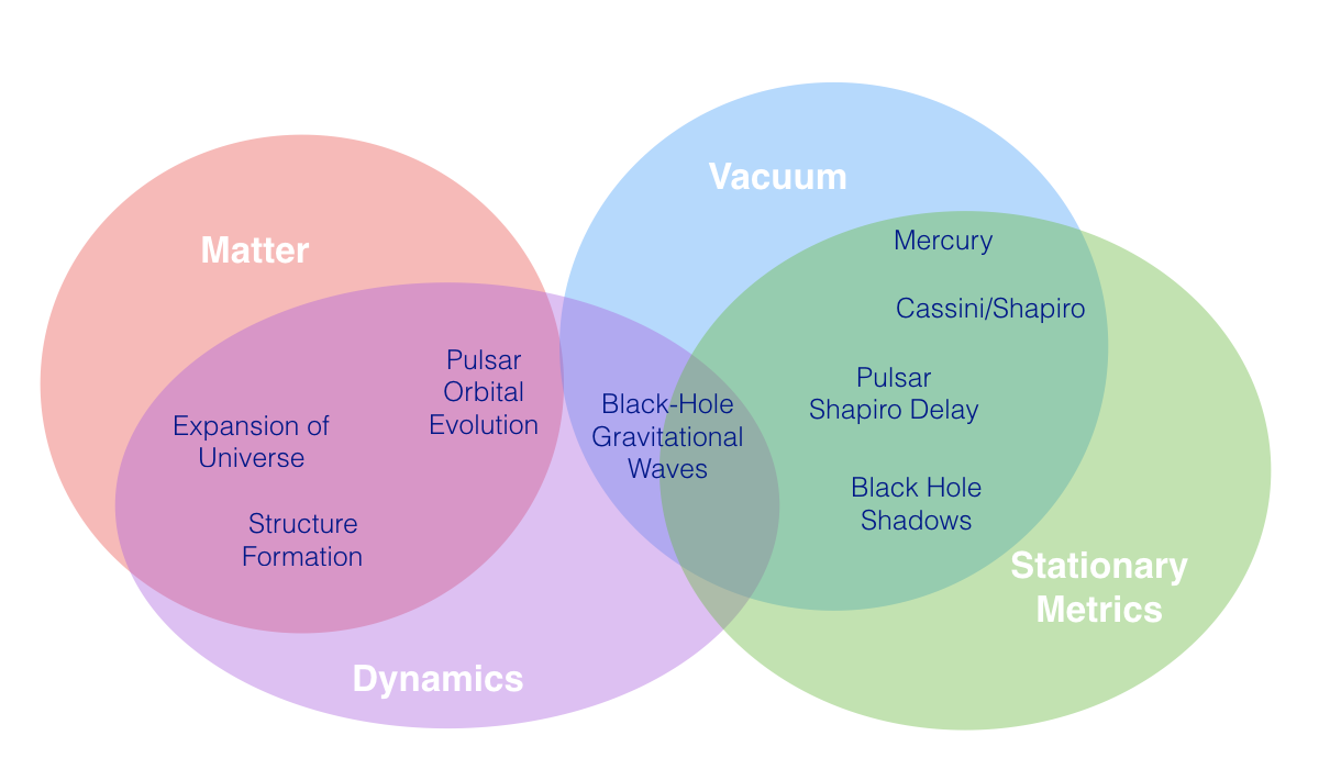
6.1 The Gravitational Field Probed by the Image of Sgr A^∗

There exist a number of key qualitative differences between the aspects of the theory of gravity probed by various tests of General Relativity. For example, as Figure 22 illustrates, some of the tests are sensitive primarily to the dynamics and propagating modes of the gravitational fields, as is the case with pulsar timing, gravitational waves, and cosmology. Other tests involve primarily measurements of photons in stationary spacetimes, as is the case of black-hole images and stellar orbits. Some tests involve orbits of massive particles, while others involve the propagation of photons in relativistic spacetimes. Moreover, tests performed with neutron stars and in cosmological settings also probe the coupling of matter to the gravitational field, whereas black-hole and most Solar-system tests are only sensitive to the properties of vacuum spacetimes.

Figure 23: A parameter space of tests of gravity with astrophysical and cosmological systems (after Baker et al. 2015). For the Solar System and pulsar tests, the straight lines connect the range of gravitational fields that could affect, in principle, the outcome of each test, from the location of the outermost probe to the location of the central massive object; the dashed region of the cyan line indicates that the connection to the largest curvatures is theory-specific. The green lines connect the range of gravitational fields probed by two gravitational-wave tests with black-hole inspirals. Filled areas show the typical range of gravitational fields probed by (orange) cosmological, (green) gravitational-wave, and (magenta) black-hole imaging tests. Even though different tests explore, in principle, different aspects of the gravitational theory, as Figure 22 illustrates, they also probe vastly different scales. In particular, the horizon-scale images of Sgr A^∗ that we report here probe a previously unexplored region of this parameter space of gravitational physics tests.

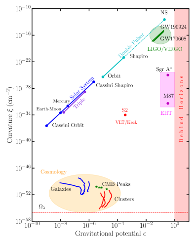
Even within these qualitative distinctions, different tests probe vastly different regimes of gravitational potential and curvature, because of the large range of masses and length scales involved. This is illustrated in Figure 23, following Baker et al. (2015). The horizontal axis in this figure shows the gravitational potential probed by each test; in the case of a test at distance $r$ from a Newtonian object of mass $M$, this dimensionless potential is equal to $\epsilon=GM/rc^{2}$. The vertical axis shows the spacetime curvature probed by each test, defined as the square root of the Kretschmann scalar; for a test in the Schwarzschild spacetime of an object, this is equal to $\xi=\sqrt{48}GM/r^{3}c^{2}$ (see Baker et al. 2015).

In order to highlight explicitly the fact that any test may probe a range of potentials and curvatures, we use straight lines to connect the smallest and largest potential and curvature that, in principle, may affect the outcome of each test. For example, in the case of the solar-System test with the Cassini spacecraft (Bertotti et al., 2003), the Shapiro delay of radio signals was measured between the Earth and the spacecraft, when the latter was between Jupiter and Saturn and as these signals grazed the surface of the Sun; this test, therefore, probes the entire range of gravitational potentials and curvatures from the solar surface to the location of the Cassini spacecraft. We also use dashed lines to connect regions of the parameter space that may affect the outcome of a test, but in a theory-specific manner. For example, in double pulsar tests, the evolution of the orbital period caused by the emission of gravitational waves probes directly the potential and curvature at the orbital separation. However, in numerous modifications of the theory of gravity, enhanced rate of emission of gravitational waves becomes possible because of the coupling of neutron-star matter to the gravitational field at the highest potential and curvature (see, e.g., Damour & Esposito-Farese 1993). In other words, depending on the particular modification of gravity that is being tested, the test involving the evolution of the binary period may probe the entire range of field strengths covered by the solid and dashed cyan lines in Figure 23.

As we will discuss below, these qualitative and quantitative differences between tests of gravity complicate our ability to cross compare and combine their results. However, these same differences also allow us to leverage the broad range of conditions that various tests probe in order to draw conclusions about the theory of gravity that could not have been reached by any test individually. For example, one of the key predictions of General Relativity is that the spacetime properties of black hole scale with their mass. This is a prediction that we can test by comparing the results of gravitational-wave tests that probe stellar-mass black holes to those of the imaging tests that probe supermassive black holes. At the same time, General Relativity predicts that, according to Birkhoff’s theorem, the external spacetime of a slowly spinning object is independent of its internal structure and composition. We will test this prediction by comparing the results of black-hole tests to those that involve pulsars or the Sun.

6.2 Comparing Gravitational Tests Across Scales

Because of their qualitative differences, every type of test of General Relativity is performed with a unique theoretical framework that is optimal for the system under study. Solar-System tests use Parametrized Post-Newtonian (PPN) expansions (Will, 2014), pulsar tests use post-Keplerian parametrizations and also a strong-field equivalent of the PPN-formulation (see, e.g., Wex & Kramer 2020), shadow tests use parametric post-Kerr metrics (Johannsen & Psaltis, 2011; Johannsen, 2013a; Vigeland et al., 2011; Rezzolla & Zhidenko, 2014; Konoplya et al., 2016), gravitational-wave tests with inspirals use post-Newtonian (Khan et al., 2016), effective-one-body (Buonanno & Damour, 1999, 2000), parametrized post-Einstein (ppE) frameworks (Yunes & Pretorius, 2009), etc. Unfortunately, this plurality of methods restricts our ability to combine and leverage the results of different tests since, in many cases, the parameters of each framework are not directly related to each other.

In principle, there are two ways we can combine tests across different scales and systems. In one approach, we can use a particular class of theories (e.g., scalar-tensor gravity) and compare the constraint of the parameters of that class from different tests. This is the most direct approach that requires typically no additional assumptions to be made. However, it is limited to the particular alternative to General Relativity that are described by the theory under study. In a second approach, as a practical solution, we can make simplifying assumptions (e.g., that the dynamics of the theory are the same as in General Relativity but the stationary spacetimes are not) and constrain phenomenological parameters of the metrics of the objects involved.

In order to make the latter approach independent of coordinate systems or gauges, and focusing here on tests of stationary metrics, we often convert the bounds on the parameters of a particular framework to constraints on the effective post-Newtonian parameters of the metrics of the objects involved. Within the particular assumptions inherent to each test, this approach is formally correct, even if one uses tests in the strong-field regime, as long as the framework used to obtain these constraints is itself applicable in that regime. Moreover, in doing so, there is no implicit assumption that the derived post-Newtonian parameters are universal constants. Indeed, in most modifications to General Relativity, the values of these parameters are specific to the situation under consideration, as they may depend on the strength of the gravitational field (curvature or potential) probed, the nature of the compact object (binary or not, with matter or pure vacuum, etc.), and the boundary conditions (the coupling of matter to the field at the center of the system, the asymptotic cosmological boundary conditions, the cosmic time of the test, etc.). This is the reason why it is important to measure potential deviations of such parameters in different astrophysical and cosmological settings that span a wide range of masses and physical conditions, as shown in Figure 23.

6.3 Tests with the S2 Orbit

Sgr A^∗ is unique in enabling us to probe the metric of the same black hole both at horizon scales, with the EHT images reported here, as well as at larger distances, with the orbits of S-stars. In performing the imaging test in Section 3.5, we have already used the measurement of the mass-to-distance ratio for the black hole that was obtained through monitoring the S-star orbits. In spacetime terms, this Keplerian mass is simply the coefficient of the asymptotic, Newtonian expansion of the metric. However, recent measurements of relativistic effects in the stellar orbits resulted in constraints on the metric properties beyond the Newtonian regime, which we explore here.

The motions of several S-stars have been monitored for almost three decades with adaptive optics instruments on VLT and Keck and their orbits have been well determined (see, e.g., Ghez et al. 2008; Gillessen et al. 2009b). The detection of gravitational redshift (Gravity Collaboration et al., 2018a; Do et al., 2019) and of the precession of the periapsis (Gravity Collaboration et al., 2020a) in the S0-2 orbit has led to tests of the equivalence principle and of the Schwarzschild metric (Section 2; see also Hees et al. 2017; Amorim et al. 2019). Because in the gravitational test we report here with the Sgr A^∗ images we explicitly assume the validity of the equivalence principle and only test the metric, we will focus on the connection of the imaging to the post-Newtonian tests of the metric using the precession of the S0-2 orbit.

In Gravity Collaboration et al. (2020a), the measured rate of precession of the S0-2 orbit was quantified through a phenomenological parameter $f_{\rm SP}$, such that the precession per orbit at the first post-Newtonian order can be written as

$$\Delta\phi_{\mathrm{1}}=f_{\rm SP}\frac{6\pi GM}{a(1-e^{2})c^{2}}\;,$$ (24)

where $a$ and $e$ are the orbital separation and eccentricity of the orbit, respectively. The best-fit value for $f_{\rm SP}$ was found to be consistent with the predictions of the Schwarzschild metric, i.e., $f_{\rm SP}=1.1\pm 0.19$.

In the PPN formalism, the phenomenological parameter $f_{\rm SP}$ is related to two of the first-order post-Newtonian parameters of the metric via (Will, 2014)

$$f_{\rm SP}=\frac{1}{3}\left(2+2\gamma_{\rm S0-2}-\beta_{\rm S0-2}\right)\;,$$ (25)

such that

$$2\gamma_{\rm S0-2}-\beta_{\rm S0-2}=1.3\pm 0.57\;.$$ (26)

Here the subscripts explicitly denote the fact that these parameters are not universal constants but are specific to the metric of Sgr A^∗ as measured at the location of the S0-2 orbit. In deriving this equation, we have also assumed that the mass of the S0-2 star is negligible with respect to the black-hole mass (see eq. [32] below).

We now assess the freedom these observations allow for possible deviations at higher post-Newtonian orders and hence the leverage of the strong-field imaging tests that we report here in constraining the metric of Sgr A^∗. We first write the precession per orbit at the second post-Newtonian orbit as (Will, 2018)

$$\Delta\phi_{2}=-6\pi\left[\frac{GM}{2a(1-e^{2})c^{2}}\right]^{2}(10-e^{2})\;.$$ (27)

The ratio of the second to the first order post-Newtonian term for the S0-2 star is

$$\frac{\Delta\phi_{2}}{\Delta\phi_{1}}=\frac{GM}{4a(1-e^{2})c^{2}}(10-e^{2})\simeq 7\times 10^{-4}\;.$$ (28)

Because the first post-Newtonian term has been measured to an accuracy of $\sim 20$% (see eq. [26]), the second post-Newtonian term would have to be $\sim 0.2/7\times 10^{-4}\simeq 285$ times larger than the Schwarzschild prediction in order for it to cause deviations detectable with current instruments. We will consider this as a heuristic upper bound on possible deviations at the second post-Newtonian order imposed by the precession of the S0-2 orbit.

Had the metric of Sgr A^∗ deviated from Schwarzschild by, e.g., a factor of 250 at the second post-Newtonian order, this would have still been undetectable by the S0-2-precession test but would have led to a shadow size as large as $\sim 85GM/c^{2}\simeq 425~{}\mu$as (see eq. [33] of Psaltis et al. 2021). This predicted size would have been at least a factor of 8 larger than the measured size we report in Section 3.5 and, more importantly, would have been almost two orders of magnitude larger than any potential uncertainty introduced by systematics due to plasma physics (as captured by the $\alpha_{1}-1$ factor) or due to our measurement methods (as captured by the $\alpha_{2}-1$ factor). In other words, the horizon-scale images of Sgr A^∗ provide substantial constraints to potential deviations of the black-hole spacetime from the GR predictions that could have evaded all prior bounds, beyond any astrophysical uncertainties.

Figure 24: Comparison of the posterior distributions for the fractional deviation $\delta$ from the Schwarzschild predictions, as inferred by the EHT measurement of the size of the black-hole shadows in Sgr A^∗ and M87. The purple-shaded area shows the $\sim 8$% range predicted for the Kerr metric, depending on the black-hole spin and observer inclination. The red-shaded area shows the small range of posteriors for Sgr A^∗, inferred with different imaging and calibration algorithms (see Fig. 12). The solid and dashed lines show the posteriors for the M87 black hole, when the stellar- and gas-dynamics measurements of the mass-to-distance ratio have been used, respectively. The negligible uncertainties in the mass measurement of Sgr A^∗, which is the result of the detection of relativistic effects in the orbit of the S0-2 star, removes any ambiguity in the comparison with the Kerr predictions.

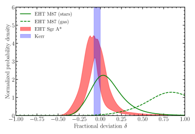
6.4 M87 Imaging Tests

The black hole at the center of the M87 galaxy has a mass that is approximately 1500 times larger than the one in Sgr A^∗. As a result, observations of horizon-scale images from the M87 black hole probe similar potentials but curvatures that are 6 orders of magnitude smaller than those of Sgr A^∗. In Event Horizon Telescope Collaboration et al. (2019c), we used the 2017 EHT images of the M87 black hole to derive constraints on possible deviations of the inferred size of the black hole shadow from the Schwarzschild prediction and, in Psaltis et al. (2020a) and Kocherlakota et al. (2021), we used these measurements to place constraints on possible deviations of metric parameters from Kerr.

Contrary to the case of Sgr A^∗ that we report here, there were two independent and distinct priors on the mass-to-distance ratio for the black hole in M87, based on either stellar- (Gebhardt et al., 2011) or gas-dynamic measurements (Walsh et al., 2013). Adopting the former resulted in an upper bound on deviations from the Kerr predictions that was consistent with zero, within $\sim 17$%. We opted to assign negligible prior likelihood to the latter prior, as it would have led us to conclude that there is significant tension between the Kerr predictions and the observations, and instead used the measurements as a null hypothesis test, i.e., concluded that the EHT images were not inconsistent with the Kerr predictions.

Figure 24 compares the posteriors on the deviation parameter $\delta$ obtained here for Sgr A^∗ to those reported earlier for the M87 black hole. In the case of the image in Sgr A^∗, we have a precise measurement of the mass-to-distance ratio for the black hole based on the detection of relativistic effects in the orbit of the S0-2 star, as discussed in Section 2. This removes any ambiguity in our calculation of the Kerr predictions. Moreover, the uncertainties in the mass-to-distance priors for Sgr A^∗ are negligible compared to those in M87, even if we only adopt the stellar-dynamic measurement for the latter. This results in uncertainties on the bounds of the deviation parameter $\delta$ that are almost a factor of 2 smaller in Sgr A^∗ compared to the M87 black hole.

In both the Sgr A^∗ and M87 cases, the inferred sizes of the black-hole shadows are consistent with the Kerr predictions, even though the black holes span 3 orders of magnitude in mass and 6 orders in curvature scale. This serves as a confirmation of the General Relativistic prediction that the spacetime properties of black holes scale with their mass and can be further reinforced by leveraging tests that involve stellar-mass black holes, as we discuss bellow.

6.5 Gravitational Wave Tests

Observations of gravitational waves from coalescing black-hole binaries with LIGO/Virgo provide strong-constraints on potential near-horizon modifications of the predictions of the theory of gravity for black holes (Abbott et al., 2016, 2019, 2021). Because of the frequency range of these ground-based gravitational-wave detectors, the black-hole masses they are sensitive to are in the $10-100~{}M_{\odot}$ range. As a result, compared to the tests with the EHT black-hole images, existing gravitational wave observations probe similar potentials but curvatures that are different by 8-16 orders of magnitude.

A second important difference arises from the fact that, fundamentally, gravitational-wave observations measure the propagating gravitational modes of the theory, whereas black-hole images measure electromagnetic modes propagating on the black-hole spacetimes. It is possible that the number and polarization of the propagating modes of the fundamental theory of gravity are the same as those in General Relativity but the stationary metrics are not; in fact, it is possible that the fundamental theory of gravity is General Relativity but the stationary metrics of the supermassive compact objects in the centers of galaxies are not described by the Kerr metric (see, e.g., Gair et al. 2008). Alternatively, it is possible that the propagating modes of the theory are very different than those in General Relativity but the stationary spacetimes remain Kerr (Psaltis et al., 2008; Barausse & Sotiriou, 2008). In this way, the gravitational-wave and imaging observations of black holes provide complementary probes of potential modifications to General Relativity.

Figure 25: Comparison of the posterior distributions for the fractional deviation $\delta$ from the Schwarzschild predictions, as inferred by the EHT measurement of the size of the black-hole shadow in Sgr A^∗ (red curve for the fiducial priors) and M87 (green curve for the stellar-dynamics mass) as well as by the LIGO/Virgo measurements of the inspiral phases of GW170608 (blue) and GW190924 (orange). The posteriors corresponding to the latter two reflect the prediction on the fractional deviation $\delta$ in the shadow size one would have calculated based on the constraints imposed by the gravitational-wave measurements, if the coalescing, stellar-mass sources had the same form of metrics as those of the supermassive black holes observed with the EHT. The gray-shaded area shows the $\sim 8$% range predicted for the Kerr metric, depending on the black-hole spin and observer inclination. Even though tests with gravitational waves and black-hole images span black-hole masses that are different by 8 orders of magnitude, they are all consistent with the GR predictions that all black holes are described by the same metric, independent of their mass.

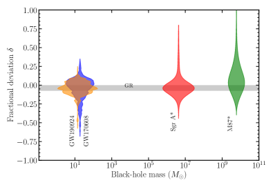
Because of this fundamental difference, however, in order to compare directly gravitational-wave constraints to those of black-hole imaging, one needs to make specific assumptions. Our main goal in this section is to leverage the gravitational-wave tests in order to assess whether the black-hole metric properties scale with mass, as predicted by General Relativity. For this reason, we will focus on the inspiral phases of the observed gravitational waves, as these are ones that are mostly sensitive to modifications in the metrics of the coalescing black holes (see, also, Völkel & Barausse 2020). Moreover, following Psaltis et al. (2021), we will assume here that the propagating modes of the theory are indistinguishable from those in General Relativity and assign any room for potential deviations to changes in the underlying metrics of the black holes. Unless the fundamental theory of gravity is finely tuned such that the modifications in the radiative sector exactly cancel those in the metrics, for the masses of the LIGO/Virgo black holes, our constraints will represent broad-brush upper limits on potential metric deviations.

Under the assumptions outlined above, the LIGO/Virgo measurements of the inspiral phases of coalescing black-hole binaries depend entirely on the $tt-$components of the metrics, as expressed in areal coordinates (Carson & Yagi, 2020; Cárdenas-Avendaño et al., 2020). This is a consequence of the fact that the waveforms of the gravitational waves during the decay of quasi-circular orbits are determined by the binding energies of the orbits and their angular frequencies (see, e.g., eq. [9] of Carson & Yagi 2020), both of which are determined by the $tt-$components of the metric (Ryan, 1995). This is the same component of the metric that determines the size of the black-hole shadows measured with the EHT (Psaltis et al., 2020a). Remarkably, because of a coincidence related to the masses of the coalescing black holes, the degeneracies between the constraints from inspiral measurements on the various parameters of metrics that deviate from Kerr are nearly parallel to those of the constraints imposed from the EHT imaging observations (Psaltis et al., 2021). In other words, this coincidence allows us to use the LIGO/Virgo constraints and make a prediction on the fractional deviation $\delta$ in the shadow-size one would have calculated, if the gravitational-wave sources had the same metrics as those of the supermassive black hole observed with the EHT.

Figure 25 compares the results on the deviation parameter $\delta$ for the two most constraining gravitational-wave events, GW170608 and GW190924 (Psaltis et al., 2021), to those obtained in §3.5 for Sgr A^∗, as well as those for the M87 black hole derived earlier (Event Horizon Telescope Collaboration et al., 2019c). As discussed above, all observations are consistent with the predictions of General Relativity, even though they utilize black holes with masses that are different by 8 orders of magnitude. This lends support not only to the Kerr nature of the black-hole spacetimes but also to the fact that the fundamental theory of gravity does not have a scale between those probed by stellar-mass and supermassive black holes.

6.6 Pulsar Timing Tests

The potentials and curvatures probed by pulsar timing tests may depend on the underlying theory of gravity, as discussed above. In principle, in theories without a characteristic scale (such as screening) between the orbital separation of the binary and the size of the neutron star, pulsar tests probe the coupling of matter to the gravitational field, which takes place in the strong field regime of the neutron-star interior, i.e., at a potential of order unity and curvature of order $10^{-10}$ cm^-2. For such theories, the horizon-scale images of Sgr A^∗ probe a similar potential but a curvature that is different by 15 orders of magnitude (see Fig. 23).

In contrast, theories with a characteristic scale between the orbital separation of the binary and the size of the neutron star (or other similar effects as in Yagi et al. 2016) are only probed at the potential of the periapsis distance for tests involving the orbital period derivative and orbital precession (for the double pulsar this is about $6\times 10^{4}GM/c^{2}$) or at the distance of minimum approach for the Shapiro delay (for the double pulsar, this distance is about $1500GM/c^{2}$). In this case, the horizon-scale images of Sgr A^∗ probe similar curvatures but a potential that is larger by 5 orders of magnitude.

Following these two approaches, we are going to discuss the constraints imposed on the various deviation parameters in two complementary ways. First is in a theory-agnostic way, in terms of the effective post-Newtonian parameters of the metrics of the compact objects. Second is in terms of the scalar-tensor gravity theory of Damour & Esposito-Farese (Damour & Esposito-Farese, 1993), with second-order couplings between the scalar field and the Einstein tensor defined by the parameters $\alpha_{a}\equiv\partial\ln m_{a}/\partial\phi_{0}$ and $\beta_{a}\equiv\partial\alpha_{a}/\partial\phi_{0}$, where the subscript $a$ corresponds to either the pulsar “p” or the companion “c”. In such a theory, the effective 1PN parameters can be expressed in terms of the theory parameters $\alpha_{a}$ and $\beta_{\alpha}$ as

$$\hat{\gamma}_{ab}=1-\frac{2\alpha_{a}\alpha_{b}}{1+\alpha_{a}\alpha_{b}}$$ (29)

and

$$\hat{\beta}^{a}_{bc}=1+\frac{\beta_{a}\alpha_{b}\alpha_{c}}{2(1+\alpha_{a}\alpha_{b})(1+\alpha_{a}\alpha_{c})}\;,$$ (30)

where the “hats” and subscripts emphasize the fact that the strong-field equivalents to the PPN parameters are not universal constants.

In principle, there are at least five theory-independent post-Keplerian parameters in a binary system that can be measured from pulsar timing (Damour & Taylor, 1992). Together with the normal Keplerian parameters, they comprise a set of inferred quantities that is larger than the free parameters in the system (see Wex & Kramer 2020 for a recent review). The combination of any two post-Keplerian parameters is used to determine the masses of the two objects in the binary. Any additional measurement can then be used for testing GR and a very broad class of alternative (boost-invariant) theories (Damour & Taylor, 1992; Will, 2014, 2018; De Laurentis et al., 2018). We will focus below on the constraints imposed by the measurement of Shapiro delay, of the precession of periapsis of the binary, and of the orbital period evolution caused by the emission of gravitational waves.

Shapiro delay.— Some of the main constraints on deviations from General Relativity come from the measurement of a Shapiro delay in binary pulsar systems. Like the imaging of black holes, such experiments provide rare opportunity to study the light-propagation near strongly self-gravitating objects. Two parameters can be measured, the “shape” $s$ and the “range” $r$. The Shapiro shape, $s$, can quite generally be identified with the sine of the orbital inclination (i.e., $s=\sin i$, e.g. Kramer et al. 2021) In comparison, the Shapiro range $r$ relates to the companion mass, e.g., in General Relativity one finds $r=Gm_{c}/c^{3}$.

For a theory agnostic constraint, one can relate $r$ to the 1PN parameter $\gamma$ via

$$r=\frac{\hat{G}_{0,c}m_{c}(1+\hat{\gamma}_{0c})}{2c^{3}}$$ (31)

where $m_{c}$ is the mass of the companion star and the subscript on the PN parameter makes explicit that this is the value for the coupling between a test particle and the pulsar companion, i.e. they are not universal constants but object-specific. The subscript in the gravitational constant $G$ also denotes that this is the effective gravitational constant felt by a test particle in the field of the companion.

Figure 26: Comparison of the current limits on various potential metric deviation parameters at the first post-Newtonian order obtained from different tests of gravity with astrophysical objects, as a function of the (top panel) gravitational potential and (right panel) curvature probed by each test. For visual clarity, each upper limit is calculated assuming that the deviations at all other post-Newtonian orders are negligible; this plot, therefore, represents only one cross section in the multi-dimensional parameter space of plaussible deviations. Every tests probes a different combination of post-Newtonian parameters, as shown on the upper panel. In most modifications to General Relativity, these post-Newtonian parameters are not universal constants but depend on the nature of the central object, its mass, composition, scale, etc.

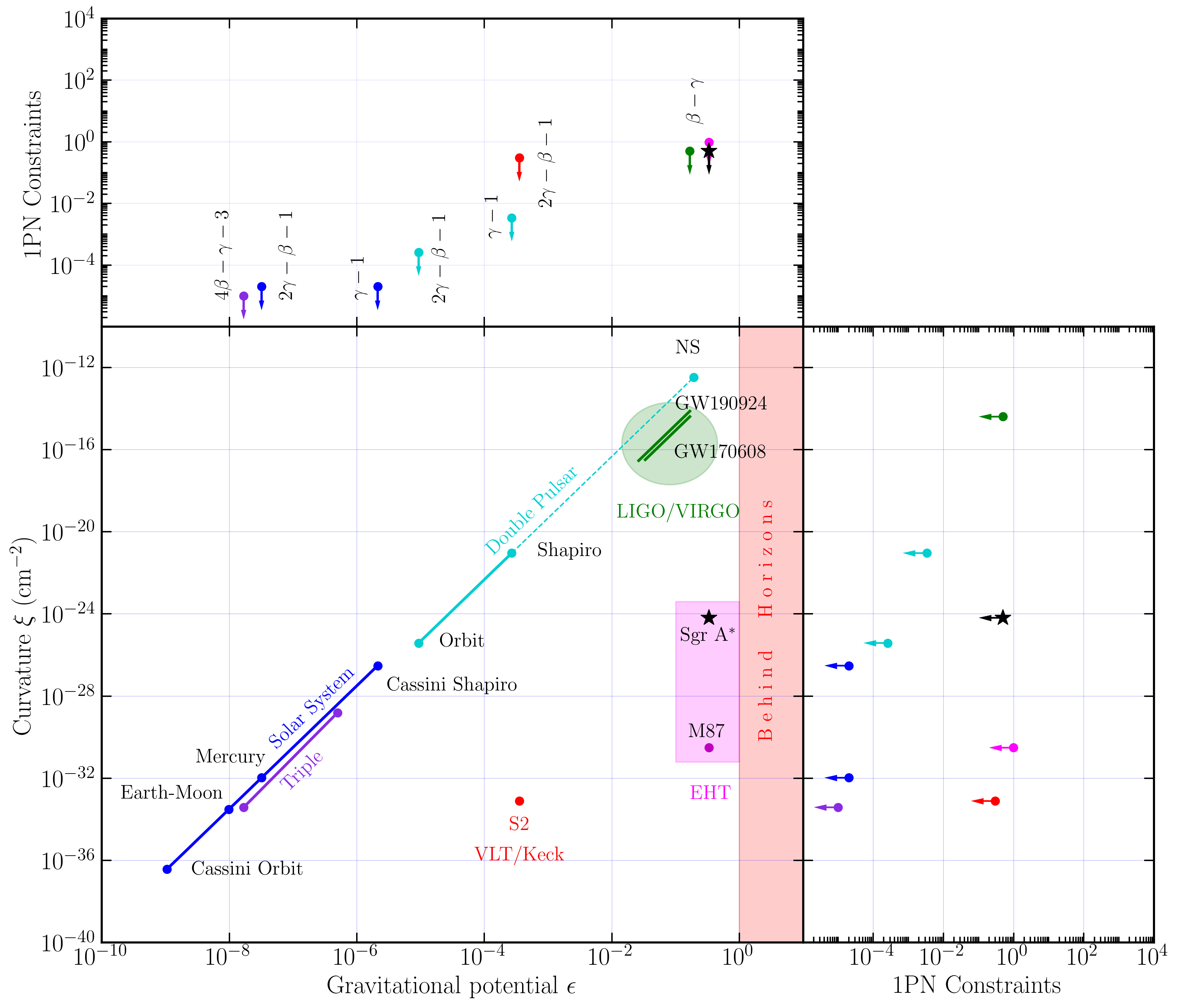
Precession of periapsis.— In GR, within the PPN framework, the rate of precession of the periapsis $\dot{\omega}$ depends on the combination $2+2\hat{\gamma}-\hat{\beta}$ (in the limit when the mass ratio is zero). Incorporating the effects due to the presence of two orbiting objects for which the strong-field coupling of matter to gravity cannot be neglected, $\dot{\omega}$ becomes proportional to

$$k=\left(2+2\hat{\gamma}_{pc}-\frac{m_{c}}{M}\hat{\beta}_{cc}^{p}-\frac{m_{p}}{M}\hat{\beta}_{pp}^{c}\right)\frac{\left(\hat{G}_{pc}Mn_{b}\right)^{2/3}}{c^{2}(1-e^{2})}\;.$$ (32)

Here $M\equiv m_{c}+m_{p}$ is the sum of the companion and pulsar masses, $m_{c}$ and $m_{p}$, respectively, and $e$ is the eccentricity of the orbit.

Orbital period derivative.— The orbital period of a binary system may change due to a number of effects. In case that only gravity plays a role, a decay in the orbital period results from the emission of gravitational waves. The measurement of an orbital period derivative can then be used to confront a given theory with its predictions. In General Relativity, to leading order, the orbital period derivative is given by the quadrupole formula (Peters, 1964). In contrast, many alternative theories of gravity violate the strong equivalence principle, resulting in the emission of gravitational dipolar radiation. Observations of binary pulsars can provide strict limits on the existence of dipolar radiation (Shao & Wex, 2016; Wex & Kramer, 2020). Indeed, the Double Pulsar system provides currently the most precise test of the General Relativistic quadrupolar description of gravitational waves, validating the prediction at a level of $1.3\times 10^{-4}$ (95% conf. level, Kramer et al. 2021).

Under the assumption that the radiative sector is negligibly different from General Relativity, one can put, in a theory agnostic way, constraints on the post-Newtonian parameters of the waveform, obtaining at 1PN order

$$\hat{\beta}-\hat{\gamma}=\Delta\phi_{2}\frac{743+924\eta}{1344}\;,$$ (33)

where $\Delta\phi_{2}$ is the 1PN order correction to the phase term of the gravitational waveform.

Following this framework, and emphasizing the mentioned assumptions, we can use the other precise measurements in the Double Pulsar system for $r$ and $\dot{\omega}$ to derive constraints on the corresponding post-Newtonian parameters at the first and second orders. At the 68% confidence limit, particular combinations of these parameters that give rise to the the Shapiro range, the periapsis advance and the orbital decay have been found to be consistent with the General Relativistic predictions at a precision of $3.4\times 10^{-3}$, $2.6\times 10^{-4}$, and $6.3\times 10^{-5}$, respectively (Kramer et al., 2021).

Universality of free fall .— One can use pulsars also to test the strong equivalence principle (SEP), as first shown by Damour & Schaefer (1991). The discovery of a pulsar in a triple system (Ransom et al., 2014) allow a variation of the Damour-Schäfer experiment in very constraining way (Freire et al., 2012). In the triple system an inner pulsar - white dwarf system is orbited by a second white dwarf in an outer orbit. By tracking the orbital motion of the neutron star via pulsar timing, one can study how the inner two objects with significantly different gravitational self-energy are falling in the gravitational field of the third object. Archibald et al. (2018) presented a limit on the strong-field equivalent of the Nordtvedt parameter of $\eta<3\times 10^{-5}$. Following Damour & Schäfer, it relates to the strong-field SEP violation parameter as

$$\Delta=\eta\epsilon_{\rm grav}+\eta\textquoteright\epsilon_{\rm grav}^{2}$$ (34)

where $\eta$ and $\eta^{\prime}$ are strong-field equivalents of the Nordtvedt parameter and $\epsilon_{\rm grav}=E_{\rm grav}/mc^{2}$ is the normalized Newtonian gravitational binding energy. At the first post-Newtonian order, the Nordtvedt parameter is related to the post-Newtonian coefficients by $|\eta|=|4\beta-\gamma-3|$. Ignoring higher terms, and using the results by Archibald et al. (2018), leads to $|4\beta-\gamma-3|<1.0\times 10^{-5}$ (95% C.L.). At the second post-Newtonian order, we make use of the Messenger limit obtained in the Solar System (Genova et al., 2018) to constrain $\eta^{\prime}<1.2\times 10^{-3}$ (95% C.L.).

6.7 Leveraging Gravitational Tests Across Different Scales

Figures 26 and 27 compare the constraints on the various metric deviation parameters at the first and second post-Newtonian orders that are imposed by the gravity tests discussed above. For visual clarity reasons alone, the figures show only a particular cross section of the multi-dimensional parameter space of plausible deviations: in constructing this figure, we have assumed that all deviation parameters other than those plotted are negligible. Barring any fine tuning of the fundamental theory that would lead to fortuitous cancellations, the bounds plotted can be regarded as rough upper limits. It is important to emphasize here that since each test probes a different combination of the various post-Newtonian parameter, which are indicated on the figure for those at the first post-Newtonian order, it is mathematically impossible for any non-Kerr metric to evade simultaneously all constraints purely by fortuitous cancellations.

The bounds on the post-Newtonian parameters that are imposed by the imaging observations of Sgr A^∗ and M87, the detection of periapsis precession in the S2 orbit, the gravitational-wave observations, and the double pulsar have been discussed in §5.3, Event Horizon Telescope Collaboration et al. (2019c), §6.3, Psaltis et al. (2021), and §6.6, respectively. The figures also incorporate the limits on the first- and second post-Newtonian parameters obtained by Solar System tests, which we briefly discuss below.

The measurement of the solar Shapiro delay with the Cassini spacecraft constrained the $\gamma_{\odot}-1$ parameter at the first post-Newtonian order with an accuracy of $\sim 2\times 10^{-5}$ (Bertotti et al., 2003). At the second post-Newtonian order, the best constraint comes from the deflection of light measurements that are consistent with the Schwarzschild predictions to an accuracy of $\sim 10^{-4}$. The second-order post-Newtonian correction for light deflection at the solar surface is of order $\sim 3\times 10^{-6}$ (Bodenner & Will, 2003). Therefore, any second-order post-Newtonian corrections to the solar metric cannot be larger than $\sim 10^{-4}/(3\times 10^{-6})\simeq 35$ times the Schwarzschild predictions.

The periastron precession of Mercury constraints the combination $2\gamma_{\odot}-\beta_{\odot}-1$ with an accuracy of $\sim 2\times 10^{-5}$. Given the strict limit on $\gamma_{\odot}$ for the Solar metric from Cassini, it can be translated into an upper bound on $\beta$ alone. Effects due to the second post-Newtonian order are subdominant compared to relativistic effects involving other Solar-System bodies and are of order $\sim 7\times 10^{-8}$ smaller than the first-order effects (Will, 2018). As a result, we can conclude that any second-order post-Newtonian corrections to the solar metric cannot be larger than $\sim 2\times 10^{-5}/(7\times 10^{-8})\simeq 300$ times the Schwarzschild predictions.

Figure 27: Same as Fig. 26 but for the constraints on the second post-Newtonian order, assuming that the deviations at all other post-Newtonian orders are negligible.

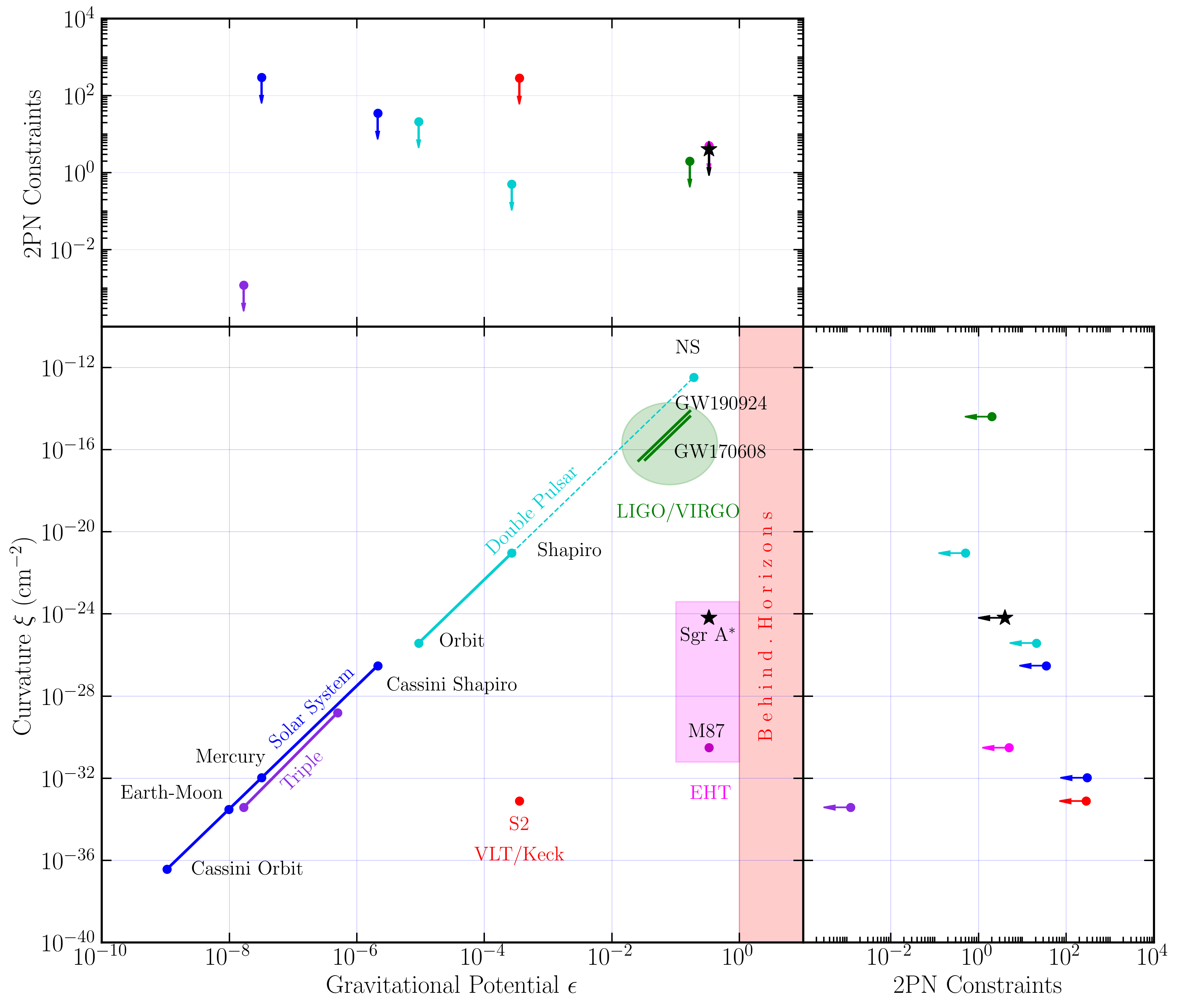
Examining the combined constraints shown in Figures 26 and 27 allows to draw some general conclusions on modifications to the equilibrium metrics of massive, isolated objects from the predictions of General Relativity that can be accommodated within current observational bounds, barring any fortuitous cancellations: (i) They may appear at the first post-Newtonian order and attain up to order-unity magnitudes at the highest gravitational potentials of compact objects but only in theories with coupling to matter that evades the theory-specific bounds imposed by the double pulsar pulsar. (ii) They may appear primarily at the second or higher post-Newtonian orders but with magnitudes that are constrained only to within order-unity deviations from the general relativistic predictions.

7 Summary

The Galactic Center black hole, Sgr A^∗, is an ideal and natural laboratory for testing the strong-field predictions of General Relativity. Monitoring of the orbits of tens of stars within its radius of influence and the recent detection of two relativistic effects in one of them has led to a precise determination of the black-hole mass and distance from the Earth (Gravity Collaboration et al., 2018a; Do et al., 2019; Gravity Collaboration et al., 2020a). Compared to any other black hole on the sky observed in the electromagnetic spectrum, these measurements lead to precise predictions for the magnitudes of gravitational effect, which can then be tested against other observations.

In this series of papers, we are reporting the first horizon-scale images of Sgr A^∗, obtained with the EHT at a wavelength of 1.3 mm (Paper II). The images are characterized by a bright ring of emission surrounded by a deep brightness depression (Paper III). This image structure is stable and remains present for at least the $\sim 32$hr span of observations on 2017 April 5-6, which corresponds to $\sim 60-500$ dynamical timescales at the radius of the innermost stable circular orbit, depending on black-hole spin. Using a variety of image-reconstruction and visibility-domain modeling tools, we measured the diameter of the ring-like structure to be equal to $50\pm XX~{}\mu$as (make consistent with Paper I).

The structure, size, and persistent nature of the black-hole image leads us to identify the central brightness depression with the shadow that the black hole is expected to cast on the emission from the accreting plasma. Using the depth and size of this brightness depression as well as the observed broadband spectrum of the source, we rule out the possibility that Sgr A^∗ has either a surface that fully absorbs and remits thermally the incoming energy flux or that it has a reflecting surface at 1.3 mm with significant albedo.

Using an extensive suite of images and synthetic data based on time-dependent and semi-analytic plasma models in a variety of spacetimes, we calibrated the difference between the size of the observed emission ring and that of the shadow as well as potential systematic effects introduced by the sparse interferometric coverage of the EHT array and our analysis methods. We found the magnitudes of these effects to be of order $\sim 10$%. This is subdominant compared to the significantly larger effect caused by changing the spacetime of Sgr A^∗, which can be as large as an order of magnitude while remaining consistent with the bounds imposed by the observation of the orbit of the S0-2 star in the spacetime of the same black hole.

Because in the Kerr metric the size of the shadow depends primarily on the mass-to-distance ratio of the black hole, which is well determined by monitoring of stellar orbits, we can compare directly the predicted Kerr size to the observations, without any free parameters. We find that the Kerr predictions are consistent with observations at the $\sim 10$% level. We then use this strong-field inference to place bounds of order unity to the parameters of metrics that deviate from Kerr.

The $\sim 4\times 10^{6}M_{\odot}$ mass of Sgr A^∗ places these tests of the Kerr metric in a region of the parameter space of gravitational objects that has never been probed before in the strong field regime. This mass is approximately 5 orders of magnitude larger than the masses of the objects probed by LIGO/Virgo via the detection of gravitational waves and a factor of 1500 smaller than the mass of the black hole in M87. Leveraging the fact that similar bounds on the strong-field predictions of General Relativity have been placed by gravitational-wave and imaging observations across these 8 orders of magnitude range in mass, we conclude that it is unlikely for the fundamental theory of gravity to possess a scale in this range.

These conclusions are based predominantly on the identification of the central brightness depression with the shadow of the black hole and, at the $\sim 10$% level, on the calibration of the relative size of the bright ring of emission, which we measure, to that of the shadow, which we infer. In the case of the tests involving the image of the M87 black hole that we reported earlier (Event Horizon Telescope Collaboration et al., 2019c; Psaltis et al., 2020a; Kocherlakota et al., 2021), two issues related to that black hole left open the possibility that the observed brightness depression might not have been related to the black-hole shadow. First is the factor of $\sim 2$ difference in the prior measurements of the black-hole mass based on stellar and gas dynamics (Gebhardt et al., 2011; Walsh et al., 2013). It could have been possible, in principle, for (i) the brightness depression to not be related to the black-hole shadow but be generated, for example, at a larger distance from the black hole and (ii) for the black-hole mass to be smaller than that inferred from stellar dynamics in such a way that, by pure coincidence, the size of the brightness depression is equal to the size inferred observationally. This is the approach taken, e.g., by Gralla et al. (2019) (see also Gralla et al. 2019, 2020). Second is the fact that the time spread of the M87 observations was comparable to the dynamical timescale at its innermost stable circular orbit, allowing for the possibility that the image structure observed was transient and did not correspond to the persistent image of the bright ring surrounding the black-hole shadow.

In the case of the Sgr A^∗ images, neither of these considerations provide reasonable alternatives to our interpretation. Indeed, the mass of the black hole in Sgr A^∗ is known to such a degree of precision that leaves very little room for uncertainties in the predicted diameter of the black-hole shadow. At the same time, the relatively small value of this mass, compared to the M87 black hole, allows us to observe the image over tens to hundreds of dynamical timescales and conclude that this structure is persistent and not transient. With these potential sources of uncertainty under control, we measured the size of the black-hole shadow in Sgr A^∗ and found it to be in agreement with the Kerr prediction, as we did for the case of the M87 black hole. In order to argue that the observed brightness depression is not related to the black-hole shadow, we would have to assign this consistency not only to coincidence but also require that the same coincidence works for both M87 and Sgr A^∗. Given that the two black holes have masses that are different by a factor of $\sim 1500$, are accreting at widely different rates with one showing a prominent jet that is missing from the other, and are probably observed at different inclinations, we consider this alternative to be highly unlikely.

References

- Abbott et al. (2016) Abbott, B. P., Abbott, R., Abbott, T. D., et al. 2016, Phys. Rev. Lett., 116, 221101, doi: 10.1103/PhysRevLett.116.221101
- Abbott et al. (2019) —. 2019, Phys. Rev. D, 100, 104036, doi: 10.1103/PhysRevD.100.104036
- Abbott et al. (2021) Abbott, R., Abbott, T. D., Abraham, S., et al. 2021, Phys. Rev. D, 103, 122002, doi: 10.1103/PhysRevD.103.122002
- Abdujabbarov et al. (2016) Abdujabbarov, A., Amir, M., Ahmedov, B., & Ghosh, S. G. 2016, Phys. Rev. D, 93, 104004, doi: 10.1103/PhysRevD.93.104004
- Abedi et al. (2017) Abedi, J., Dykaar, H., & Afshordi, N. 2017, Phys. Rev. D, 96, 082004, doi: 10.1103/PhysRevD.96.082004
- Abramowicz et al. (2002) Abramowicz, M. A., Kluźniak, W., & Lasota, J. P. 2002, A&A, 396, L31, doi: 10.1051/0004-6361:20021645
- Amorim et al. (2019) Amorim, A., Bauböck, M., Berger, J. P., et al. 2019, Phys. Rev. Lett., 122, 101102, doi: 10.1103/PhysRevLett.122.101102
- An et al. (2005) An, T., Goss, W. M., Zhao, J.-H., et al. 2005, ApJ, 634, L49, doi: 10.1086/498687
- Archibald et al. (2018) Archibald, A. M., Gusinskaia, N. V., Hessels, J. W. T., et al. 2018, Nature, 559, 73, doi: 10.1038/s41586-018-0265-1
- Ayón-Beato & García (1998) Ayón-Beato, E., & García, A. 1998, Phys. Rev. Lett., 80, 5056, doi: 10.1103/PhysRevLett.80.5056
- Ayón-Beato & García (2000) —. 2000, Physics Letters B, 493, 149, doi: 10.1016/S0370-2693(00)01125-4
- Baganoff et al. (2001) Baganoff, F. K., Bautz, M. W., Brandt, W. N., et al. 2001, Nature, 413, 45, doi: 10.1038/35092510
- Baker et al. (2017) Baker, T., Bellini, E., Ferreira, P. G., et al. 2017, Phys. Rev. Lett., 119, 251301, doi: 10.1103/PhysRevLett.119.251301
- Baker et al. (2015) Baker, T., Psaltis, D., & Skordis, C. 2015, ApJ, 802, 63, doi: 10.1088/0004-637X/802/1/63
- Ball et al. (2021) Ball, D., Özel, F., Christian, P., Chan, C.-K., & Psaltis, D. 2021, ApJ, 917, 8, doi: 10.3847/1538-4357/abf8ae
- Ball et al. (2016) Ball, D., Özel, F., Psaltis, D., & Chan, C.-k. 2016, ApJ, 826, 77, doi: 10.3847/0004-637X/826/1/77
- Bambi (2013) Bambi, C. 2013, Phys. Rev. D, 87, 084039, doi: 10.1103/PhysRevD.87.084039
- Barausse & Sotiriou (2008) Barausse, E., & Sotiriou, T. P. 2008, Phys. Rev. Lett., 101, 099001, doi: 10.1103/PhysRevLett.101.099001
- Bardeen (1968) Bardeen, J. 1968, in Proceedings of GR5, Tbilisi, USSR, 174
- Bardeen (1973) Bardeen, J. M. 1973, in Black Holes (Les Astres Occlus), 215–239
- Bertotti et al. (2003) Bertotti, B., Iess, L., & Tortora, P. 2003, Nature, 425, 374, doi: 10.1038/nature01997
- Bodenner & Will (2003) Bodenner, J., & Will, C. M. 2003, American Journal of Physics, 71, 770, doi: 10.1119/1.1570416
- Boehle et al. (2016) Boehle, A., Ghez, A. M., Schödel, R., et al. 2016, ApJ, 830, 17, doi: 10.3847/0004-637X/830/1/17
- Bower et al. (2015) Bower, G. C., Markoff, S., Dexter, J., et al. 2015, ApJ, 802, 69, doi: 10.1088/0004-637X/802/1/69
- Bower et al. (2019) Bower, G. C., Dexter, J., Asada, K., et al. 2019, ApJ, 881, L2, doi: 10.3847/2041-8213/ab3397
- Brinkerink et al. (2021) Brinkerink, C., Falcke, H., Brunthaler, A., & Law, C. 2021, arXiv e-prints, arXiv:2107.13402. https://arxiv.org/abs/2107.13402
- Brinkerink et al. (2015) Brinkerink, C. D., Falcke, H., Law, C. J., et al. 2015, A&A, 576, A41, doi: 10.1051/0004-6361/201424783
- Broderick et al. (2009) Broderick, A. E., Loeb, A., & Narayan, R. 2009, ApJ, 701, 1357, doi: 10.1088/0004-637X/701/2/1357
- Broderick & Narayan (2006) Broderick, A. E., & Narayan, R. 2006, ApJ, 638, L21, doi: 10.1086/500930
- Broderick & Narayan (2007) —. 2007, Classical and Quantum Gravity, 24, 659, doi: 10.1088/0264-9381/24/3/009
- Broderick et al. (2015) Broderick, A. E., Narayan, R., Kormendy, J., et al. 2015, ApJ, 805, 179, doi: 10.1088/0004-637X/805/2/179
- Bronzwaer & Falcke (2021) Bronzwaer, T., & Falcke, H. 2021, ApJ, 920, 155, doi: 10.3847/1538-4357/ac1738
- Buonanno & Damour (1999) Buonanno, A., & Damour, T. 1999, Phys. Rev. D, 59, 084006, doi: 10.1103/PhysRevD.59.084006
- Buonanno & Damour (2000) —. 2000, Phys. Rev. D, 62, 064015, doi: 10.1103/PhysRevD.62.064015
- Carballo-Rubio et al. (2018) Carballo-Rubio, R., Kumar, P., & Lu, W. 2018, Phys. Rev. D, 97, 123012, doi: 10.1103/PhysRevD.97.123012
- Cárdenas-Avendaño et al. (2020) Cárdenas-Avendaño, A., Nampalliwar, S., & Yunes, N. 2020, Classical and Quantum Gravity, 37, 135008, doi: 10.1088/1361-6382/ab8f64
- Cardoso & Pani (2019) Cardoso, V., & Pani, P. 2019, Living Reviews in Relativity, 22, 4, doi: 10.1007/s41114-019-0020-4
- Carson & Yagi (2020) Carson, Z., & Yagi, K. 2020, Phys. Rev. D, 101, 084050, doi: 10.1103/PhysRevD.101.084050
- Carter (1968) Carter, B. 1968, Physical Review, 174, 1559, doi: 10.1103/PhysRev.174.1559
- Carter (1971) —. 1971, Phys. Rev. Lett., 26, 331, doi: 10.1103/PhysRevLett.26.331
- Chael et al. (2021) Chael, A., Johnson, M. D., & Lupsasca, A. 2021, ApJ, 918, 6, doi: 10.3847/1538-4357/ac09ee
- Chael et al. (2018) Chael, A., Rowan, M., Narayan, R., Johnson, M., & Sironi, L. 2018, MNRAS, 478, 5209, doi: 10.1093/mnras/sty1261
- Chan et al. (2013) Chan, C.-k., Psaltis, D., & Özel, F. 2013, ApJ, 777, 13, doi: 10.1088/0004-637X/777/1/13
- Chapline (2003) Chapline, G. 2003, International Journal of Modern Physics A, 18, 3587, doi: 10.1142/S0217751X03016380
- Chatterjee et al. (2021) Chatterjee, K., Markoff, S., Neilsen, J., et al. 2021, MNRAS, 507, 5281, doi: 10.1093/mnras/stab2466
- Chirenti & Rezzolla (2007) Chirenti, C. B. M. H., & Rezzolla, L. 2007, Classical and Quantum Gravity, 24, 4191, doi: 10.1088/0264-9381/24/16/013
- Chu et al. (2018) Chu, D. S., Do, T., Hees, A., et al. 2018, ApJ, 854, 12, doi: 10.3847/1538-4357/aaa3eb
- Clavel et al. (2013) Clavel, M., Terrier, R., Goldwurm, A., et al. 2013, A&A, 558, A32, doi: 10.1051/0004-6361/201321667
- Cotera et al. (1999) Cotera, A., Morris, M., Ghez, A. M., et al. 1999, in Astronomical Society of the Pacific Conference Series, Vol. 186, The Central Parsecs of the Galaxy, ed. H. Falcke, A. Cotera, W. J. Duschl, F. Melia, & M. J. Rieke, 240
- Cunha & Herdeiro (2018) Cunha, P. V. P., & Herdeiro, C. A. R. 2018, General Relativity and Gravitation, 50, 42, doi: 10.1007/s10714-018-2361-9
- Curiel (2017) Curiel, E. 2017, in Towards a Theory of Spacetime Theories, ed. D. Lehmkuhl, G. Schiemann, & E. Scholz (New York, NY: Springer New York), 43–104, doi: 10.1007/978-1-4939-3210-8_3
- Damour & Esposito-Farese (1993) Damour, T., & Esposito-Farese, G. 1993, Phys. Rev. Lett., 70, 2220, doi: 10.1103/PhysRevLett.70.2220
- Damour & Schaefer (1991) Damour, T., & Schaefer, G. 1991, Phys. Rev. Lett., 66, 2549, doi: 10.1103/PhysRevLett.66.2549
- Damour & Taylor (1992) Damour, T., & Taylor, J. H. 1992, Phys. Rev. D, 45, 1840, doi: 10.1103/PhysRevD.45.1840
- Danielsson et al. (2021) Danielsson, U., Lehner, L., & Pretorius, F. 2021, Phys. Rev. D, 104, 124011, doi: 10.1103/PhysRevD.104.124011
- Davelaar et al. (2018) Davelaar, J., Mościbrodzka, M., Bronzwaer, T., & Falcke, H. 2018, A&A, 612, A34, doi: 10.1051/0004-6361/201732025
- De Laurentis et al. (2018) De Laurentis, M., Younsi, Z., Porth, O., Mizuno, Y., & Rezzolla, L. 2018, Phys. Rev. D, 97, 104024, doi: 10.1103/PhysRevD.97.104024
- De Martino et al. (2021) De Martino, I., Della Monica, R., & De Laurentis, M. 2021, Phys. Rev. D, 104, L101502, doi: 10.1103/PhysRevD.104.L101502
- Della Monica et al. (2021) Della Monica, R., De Martino, I., & De Laurentis, M. 2021, Monthly Notices of the Royal Astronomical Society, doi: 10.1093/mnras/stab3727
- Dexter et al. (2014) Dexter, J., Kelly, B., Bower, G. C., et al. 2014, MNRAS, 442, 2797, doi: 10.1093/mnras/stu1039
- Dexter et al. (2020) Dexter, J., Tchekhovskoy, A., Jiménez-Rosales, A., et al. 2020, MNRAS, 497, 4999, doi: 10.1093/mnras/staa2288
- Dey et al. (2019) Dey, D., Kocherlakota, P., & Joshi, P. S. 2019, arXiv e-prints, arXiv:1907.12792. https://arxiv.org/abs/1907.12792
- Dicke (2019) Dicke, R. H. 2019, General Relativity and Gravitation, 51, 57, doi: 10.1007/s10714-019-2509-2
- Do et al. (2009) Do, T., Ghez, A. M., Morris, M. R., et al. 2009, ApJ, 691, 1021, doi: 10.1088/0004-637X/691/2/1021
- Do et al. (2013) Do, T., Martinez, G. D., Yelda, S., et al. 2013, ApJ, 779, L6, doi: 10.1088/2041-8205/779/1/L6
- Do et al. (2019) Do, T., Hees, A., Ghez, A., et al. 2019, Science, 365, 664, doi: 10.1126/science.aav8137
- Dodds-Eden et al. (2009) Dodds-Eden, K., Porquet, D., Trap, G., et al. 2009, ApJ, 698, 676, doi: 10.1088/0004-637X/698/1/676
- Dodds-Eden et al. (2011) Dodds-Eden, K., Gillessen, S., Fritz, T. K., et al. 2011, ApJ, 728, 37, doi: 10.1088/0004-637X/728/1/37
- Doeleman et al. (2019) Doeleman, S., Blackburn, L., Dexter, J., et al. 2019, in Bulletin of the American Astronomical Society, Vol. 51, 256. https://arxiv.org/abs/1909.01411
- Done & Gierliński (2003) Done, C., & Gierliński, M. 2003, MNRAS, 342, 1041, doi: 10.1046/j.1365-8711.2003.06614.x
- Eckart et al. (2002) Eckart, A., Genzel, R., Ott, T., & Schödel, R. 2002, MNRAS, 331, 917, doi: 10.1046/j.1365-8711.2002.05237.x
- Eckart et al. (1999) Eckart, A., Ott, T., & Genzel, R. 1999, A&A, 352, L22. https://arxiv.org/abs/astro-ph/9911011
- Eckart et al. (2006) Eckart, A., Schödel, R., Meyer, L., et al. 2006, A&A, 455, 1, doi: 10.1051/0004-6361:20064948
- Eckart et al. (2004a) Eckart, A., Baganoff, F. K., Morris, M., et al. 2004a, A&A, 427, 1, doi: 10.1051/0004-6361:20040495
- Eckart et al. (2004b) —. 2004b, A&A, 427, 1, doi: 10.1051/0004-6361:20040495
- Eisenhauer et al. (2005) Eisenhauer, F., Genzel, R., Alexander, T., et al. 2005, ApJ, 628, 246, doi: 10.1086/430667
- Event Horizon Telescope Collaboration et al. (2019a) Event Horizon Telescope Collaboration, Akiyama, K., Alberdi, A., et al. 2019a, ApJ, 875, L4, doi: 10.3847/2041-8213/ab0e85
- Event Horizon Telescope Collaboration et al. (2019b) —. 2019b, ApJ, 875, L5, doi: 10.3847/2041-8213/ab0f43
- Event Horizon Telescope Collaboration et al. (2019c) —. 2019c, ApJ, 875, L6, doi: 10.3847/2041-8213/ab1141
- Event Horizon Telescope Collaboration et al. (2022a) —. 2022a, ApJ, 875, 2
- Event Horizon Telescope Collaboration et al. (2022b) —. 2022b, ApJ, 875, 3
- Event Horizon Telescope Collaboration et al. (2022c) —. 2022c, ApJ, 875, 4
- Event Horizon Telescope Collaboration et al. (2022d) —. 2022d, ApJ, 875, 5
- Event Horizon Telescope Collaboration et al. (2022e) —. 2022e, ApJ, 875, 1
- Falcke (1999) Falcke, H. 1999, in Astronomical Society of the Pacific Conference Series, Vol. 186, The Central Parsecs of the Galaxy, ed. H. Falcke, A. Cotera, W. J. Duschl, F. Melia, & M. J. Rieke, 113. https://arxiv.org/abs/astro-ph/9909441
- Falcke et al. (1998) Falcke, H., Goss, W. M., Matsuo, H., et al. 1998, ApJ, 499, 731, doi: 10.1086/305687
- Falcke et al. (1993) Falcke, H., Mannheim, K., & Biermann, P. L. 1993, A&A, 278, L1. https://arxiv.org/abs/astro-ph/9308031
- Falcke & Markoff (2000) Falcke, H., & Markoff, S. 2000, A&A, 362, 113. https://arxiv.org/abs/astro-ph/0102186
- Falcke & Markoff (2013) Falcke, H., & Markoff, S. B. 2013, Classical and Quantum Gravity, 30, 244003, doi: 10.1088/0264-9381/30/24/244003
- Falcke et al. (2000) Falcke, H., Melia, F., & Agol, E. 2000, ApJ, 528, L13, doi: 10.1086/312423
- Fazio et al. (2018) Fazio, G. G., Hora, J. L., Witzel, G., et al. 2018, ApJ, 864, 58, doi: 10.3847/1538-4357/aad4a2
- Ferreira (2019) Ferreira, P. G. 2019, ARA&A, 57, 335, doi: 10.1146/annurev-astro-091918-104423
- Fish et al. (2020) Fish, V. L., Shea, M., & Akiyama, K. 2020, Advances in Space Research, 65, 821, doi: 10.1016/j.asr.2019.03.029
- Freire et al. (2012) Freire, P. C. C., Kramer, M., & Wex, N. 2012, Classical and Quantum Gravity, 29, 184007, doi: 10.1088/0264-9381/29/18/184007
- Frolov (2016) Frolov, V. P. 2016, Phys. Rev. D, 94, 104056, doi: 10.1103/PhysRevD.94.104056
- Fromm et al. (2021) Fromm, C. M., Mizuno, Y., Younsi, Z., et al. 2021, A&A, 649, A116, doi: 10.1051/0004-6361/201937335
- Gair & Yunes (2011) Gair, J., & Yunes, N. 2011, Phys. Rev. D, 84, 064016, doi: 10.1103/PhysRevD.84.064016
- Gair et al. (2008) Gair, J. R., Li, C., & Mandel, I. 2008, Phys. Rev. D, 77, 024035, doi: 10.1103/PhysRevD.77.024035
- Gan et al. (2021) Gan, Q., Wang, P., Wu, H., & Yang, H. 2021, Phys. Rev. D, 104, 024003, doi: 10.1103/PhysRevD.104.024003
- García et al. (1995) García, A., Galtsov, D., & Kechkin, O. 1995, Phys. Rev. Lett., 74, 1276, doi: 10.1103/PhysRevLett.74.1276
- Garcia et al. (2001) Garcia, M. R., McClintock, J. E., Narayan, R., et al. 2001, ApJ, 553, L47, doi: 10.1086/320494
- Garfinkle et al. (1991) Garfinkle, D., Horowitz, G. T., & Strominger, A. 1991, Phys. Rev. D, 43, 3140, doi: 10.1103/PhysRevD.43.3140
- Gebhardt et al. (2011) Gebhardt, K., Adams, J., Richstone, D., et al. 2011, ApJ, 729, 119, doi: 10.1088/0004-637X/729/2/119
- Genova et al. (2018) Genova, A., Mazarico, E., Goossens, S., et al. 2018, Nature Communications, 9, 289, doi: 10.1038/s41467-017-02558-1
- Genzel et al. (1997) Genzel, R., Eckart, A., Ott, T., & Eisenhauer, F. 1997, MNRAS, 291, 219, doi: 10.1093/mnras/291.1.219
- Genzel et al. (2010) Genzel, R., Eisenhauer, F., & Gillessen, S. 2010, Reviews of Modern Physics, 82, 3121, doi: 10.1103/RevModPhys.82.3121
- Genzel et al. (2000) Genzel, R., Pichon, C., Eckart, A., Gerhard, O. E., & Ott, T. 2000, MNRAS, 317, 348, doi: 10.1046/j.1365-8711.2000.03582.x
- Genzel et al. (2003a) Genzel, R., Schödel, R., Ott, T., et al. 2003a, Nature, 425, 934
- Genzel et al. (2003b) —. 2003b, ApJ, 594, 812, doi: 10.1086/377127
- Gezari et al. (2002) Gezari, S., Ghez, A. M., Becklin, E. E., et al. 2002, ApJ, 576, 790, doi: 10.1086/341807
- Ghez et al. (1998) Ghez, A. M., Klein, B. L., Morris, M., & Becklin, E. E. 1998, ApJ, 509, 678, doi: 10.1086/306528
- Ghez et al. (2000) Ghez, A. M., Morris, M., Becklin, E. E., Tanner, A., & Kremenek, T. 2000, Nature, 407, 349, doi: 10.1038/35030032
- Ghez et al. (2005a) Ghez, A. M., Salim, S., Hornstein, S. D., et al. 2005a, ApJ, 620, 744, doi: 10.1086/427175
- Ghez et al. (2005b) Ghez, A. M., Hornstein, S. D., Lu, J. R., et al. 2005b, ApJ, 635, 1087, doi: 10.1086/497576
- Ghez et al. (2008) Ghez, A. M., Salim, S., Weinberg, N. N., et al. 2008, ApJ, 689, 1044, doi: 10.1086/592738
- Gibbons & Maeda (1988) Gibbons, G. W., & Maeda, K.-I. 1988, Nuclear Physics B, 298, 741, doi: 10.1016/0550-3213(88)90006-5
- Gillessen et al. (2009a) Gillessen, S., Eisenhauer, F., Fritz, T. K., et al. 2009a, ApJ, 707, L114, doi: 10.1088/0004-637X/707/2/L114
- Gillessen et al. (2009b) Gillessen, S., Eisenhauer, F., Trippe, S., et al. 2009b, ApJ, 692, 1075, doi: 10.1088/0004-637X/692/2/1075
- Gillessen et al. (2017) Gillessen, S., Plewa, P. M., Eisenhauer, F., et al. 2017, ApJ, 837, 30, doi: 10.3847/1538-4357/aa5c41
- Goddi et al. (2017) Goddi, C., Falcke, H., Kramer, M., et al. 2017, International Journal of Modern Physics D, 26, 1730001, doi: 10.1142/S0218271817300014
- Goddi et al. (2021) Goddi, C., Martí-Vidal, I., Messias, H., et al. 2021, ApJ, 910, L14, doi: 10.3847/2041-8213/abee6a
- Gralla et al. (2019) Gralla, S. E., Holz, D. E., & Wald, R. M. 2019, Phys. Rev. D, 100, 024018, doi: 10.1103/PhysRevD.100.024018
- Gralla et al. (2020) Gralla, S. E., Lupsasca, A., & Marrone, D. P. 2020, Phys. Rev. D, 102, 124004, doi: 10.1103/PhysRevD.102.124004
- Gravity Collaboration et al. (2018a) Gravity Collaboration, Abuter, R., Amorim, A., et al. 2018a, A&A, 615, L15, doi: 10.1051/0004-6361/201833718
- Gravity Collaboration et al. (2018b) —. 2018b, A&A, 618, L10, doi: 10.1051/0004-6361/201834294
- Gravity Collaboration et al. (2019) —. 2019, A&A, 625, L10, doi: 10.1051/0004-6361/201935656
- Gravity Collaboration et al. (2020a) —. 2020a, A&A, 636, L5, doi: 10.1051/0004-6361/202037813
- Gravity Collaboration et al. (2020b) —. 2020b, A&A, 638, A2, doi: 10.1051/0004-6361/202037717
- Gravity Collaboration et al. (2020c) Gravity Collaboration, Jiménez-Rosales, A., Dexter, J., et al. 2020c, A&A, 643, A56, doi: 10.1051/0004-6361/202038283
- Gravity Collaboration et al. (2021a) Gravity Collaboration, Abuter, R., Amorim, A., et al. 2021a, A&A, 645, A127, doi: 10.1051/0004-6361/202039544
- Gravity Collaboration et al. (2021b) —. 2021b, A&A, 647, A59, doi: 10.1051/0004-6361/202040208
- GRAVITY Collaboration et al. (2021) GRAVITY Collaboration, Abuter, R., Amorim, A., et al. 2021, A&A, 654, A22, doi: 10.1051/0004-6361/202140981
- GRAVITY Collaboration et al. (2022) GRAVITY Collaboration, Abuter, R., Aimar, N., et al. 2022, A&A, 657, L12, doi: 10.1051/0004-6361/202142465
- Gurvits et al. (2021) Gurvits, L. I., Paragi, Z., Casasola, V., et al. 2021, Experimental Astronomy, 51, 559, doi: 10.1007/s10686-021-09714-y
- Haggard et al. (2019) Haggard, D., Nynka, M., Mon, B., et al. 2019, ApJ, 886, 96, doi: 10.3847/1538-4357/ab4a7f
- Harko et al. (2009) Harko, T., Kovács, Z., & Lobo, F. S. N. 2009, Phys. Rev. D, 79, 064001, doi: 10.1103/PhysRevD.79.064001
- Harlow (2016) Harlow, D. 2016, Rev. Mod. Phys., 88, 015002, doi: 10.1103/RevModPhys.88.015002
- Hawking (1972) Hawking, S. W. 1972, Communications in Mathematical Physics, 25, 152, doi: 10.1007/BF01877517
- Hawking & Ellis (1973) Hawking, S. W., & Ellis, G. F. R. 1973, The large scale structure of spacetime (Cambridge, England: Cambridge University Press)
- Hayward (2006) Hayward, S. A. 2006, Phys. Rev. Lett., 96, 031103, doi: 10.1103/PhysRevLett.96.031103
- Hees et al. (2019) Hees, A., Dehghanfar, A., Do, T., et al. 2019, ApJ, 880, 87, doi: 10.3847/1538-4357/ab2ae0
- Hees et al. (2017) Hees, A., Do, T., Ghez, A. M., et al. 2017, Phys. Rev. Lett., 118, 211101, doi: 10.1103/PhysRevLett.118.211101
- Hees et al. (2020) Hees, A., Do, T., Roberts, B. M., et al. 2020, Phys. Rev. Lett., 124, 081101, doi: 10.1103/PhysRevLett.124.081101
- Held et al. (2019) Held, A., Gold, R., & Eichhorn, A. 2019, JCAP, 2019, 029, doi: 10.1088/1475-7516/2019/06/029
- Herrnstein et al. (2004) Herrnstein, R. M., Zhao, J.-H., Bower, G. C., & Goss, W. M. 2004, AJ, 127, 3399, doi: 10.1086/420711
- Hora et al. (2014) Hora, J. L., Witzel, G., Ashby, M. L. N., et al. 2014, ApJ, 793, 120, doi: 10.1088/0004-637X/793/2/120
- Hornstein et al. (2007) Hornstein, S. D., Matthews, K., Ghez, A. M., et al. 2007, ApJ, 667, 900, doi: 10.1086/520762
- Israel (1967) Israel, W. 1967, Physical Review, 164, 1776, doi: 10.1103/PhysRev.164.1776
- Israel (1968) —. 1968, Communications in Mathematical Physics, 8, 245, doi: 10.1007/BF01645859
- Janis et al. (1968) Janis, A. I., Newman, E. T., & Winicour, J. 1968, Phys. Rev. Lett., 20, 878, doi: 10.1103/PhysRevLett.20.878
- Janssen et al. (2019) Janssen, M., Goddi, C., van Bemmel, I. M., et al. 2019, A&A, 626, A75, doi: 10.1051/0004-6361/201935181
- Jaroszynski & Kurpiewski (1997) Jaroszynski, M., & Kurpiewski, A. 1997, A&A, 326, 419. https://arxiv.org/abs/astro-ph/9705044
- Jia et al. (2019) Jia, S., Lu, J. R., Sakai, S., et al. 2019, ApJ, 873, 9, doi: 10.3847/1538-4357/ab01de
- Johannsen (2013a) Johannsen, T. 2013a, Phys. Rev. D, 88, 044002, doi: 10.1103/PhysRevD.88.044002
- Johannsen (2013b) —. 2013b, Phys. Rev. D, 87, 124017, doi: 10.1103/PhysRevD.87.124017
- Johannsen & Psaltis (2010) Johannsen, T., & Psaltis, D. 2010, ApJ, 718, 446, doi: 10.1088/0004-637X/718/1/446
- Johannsen & Psaltis (2011) —. 2011, Phys. Rev. D, 83, 124015, doi: 10.1103/PhysRevD.83.124015
- Johnson et al. (2020) Johnson, M. D., Lupsasca, A., Strominger, A., et al. 2020, Science Advances, 6, eaaz1310, doi: 10.1126/sciadv.aaz1310
- Joshi et al. (2011) Joshi, P. S., Malafarina, D., & Narayan, R. 2011, Classical and Quantum Gravity, 28, 235018, doi: 10.1088/0264-9381/28/23/235018
- Joshi et al. (2014) —. 2014, Classical and Quantum Gravity, 31, 015002, doi: 10.1088/0264-9381/31/1/015002
- Kallosh et al. (1992) Kallosh, R., Linde, A., Ortín, T., Peet, A., & van Proeyen, A. 1992, Phys. Rev. D, 46, 5278, doi: 10.1103/PhysRevD.46.5278
- Kazakov & Solodukhin (1994) Kazakov, D. I., & Solodukhin, S. N. 1994, Nuclear Physics B, 429, 153, doi: 10.1016/S0550-3213(94)80045-6
- Kerr (1963) Kerr, R. P. 1963, Phys. Rev. Lett., 11, 237, doi: 10.1103/PhysRevLett.11.237
- Khan et al. (2016) Khan, S., Husa, S., Hannam, M., et al. 2016, Phys. Rev. D, 93, 044007, doi: 10.1103/PhysRevD.93.044007
- Kocherlakota & Rezzolla (2020) Kocherlakota, P., & Rezzolla, L. 2020, Phys. Rev. D, 102, 064058, doi: 10.1103/PhysRevD.102.064058
- Kocherlakota & Rezzolla (2022) —. 2022, arXiv e-prints, arXiv:2201.05641. https://arxiv.org/abs/2201.05641
- Kocherlakota et al. (2021) Kocherlakota, P., Rezzolla, L., Falcke, H., et al. 2021, Phys. Rev. D, 103, 104047, doi: 10.1103/PhysRevD.103.104047
- Konoplya et al. (2016) Konoplya, R., Rezzolla, L., & Zhidenko, A. 2016, Phys. Rev. D, 93, 064015, doi: 10.1103/PhysRevD.93.064015
- Kramer et al. (2021) Kramer, M., Stairs, I. H., Manchester, R. N., et al. 2021, Phys. Rev. X, 11, 041050, doi: 10.1103/PhysRevX.11.041050
- Kudriashov et al. (2021) Kudriashov, V., Martin-Neira, M., Roelofs, F., et al. 2021, Chinese Journal of Space Science, 41, 211, doi: 10.11728/cjss2021.02.211
- Lambert & Le Poncin-Lafitte (2011) Lambert, S. B., & Le Poncin-Lafitte, C. 2011, A&A, 529, A70, doi: 10.1051/0004-6361/201016370
- Liu et al. (2016) Liu, H. B., Wright, M. C. H., Zhao, J.-H., et al. 2016, A&A, 593, A107, doi: 10.1051/0004-6361/201628731
- Lu et al. (2017) Lu, W., Kumar, P., & Narayan, R. 2017, MNRAS, 468, 910, doi: 10.1093/mnras/stx542
- Luminet (1979) Luminet, J. P. 1979, A&A, 75, 228
- Magueijo (2003) Magueijo, J. 2003, Reports on Progress in Physics, 66, 2025, doi: 10.1088/0034-4885/66/11/R04
- Markoff et al. (2001) Markoff, S., Falcke, H., Yuan, F., & Biermann, P. L. 2001, A&A, 379, L13, doi: 10.1051/0004-6361:20011346
- Marrone et al. (2008) Marrone, D. P., Baganoff, F. K., Morris, M. R., et al. 2008, ApJ, 682, 373, doi: 10.1086/588806
- Martins et al. (2008) Martins, F., Gillessen, S., Eisenhauer, F., et al. 2008, ApJ, 672, L119, doi: 10.1086/526768
- Mazur & Mottola (2001) Mazur, P. O., & Mottola, E. 2001, arXiv e-prints, gr. https://arxiv.org/abs/gr-qc/0109035
- McClintock et al. (2004) McClintock, J. E., Narayan, R., & Rybicki, G. B. 2004, ApJ, 615, 402, doi: 10.1086/424474
- Medeiros et al. (2020) Medeiros, L., Psaltis, D., & Özel, F. 2020, ApJ, 896, 7, doi: 10.3847/1538-4357/ab8bd1
- Menten et al. (1997) Menten, K. M., Reid, M. J., Eckart, A., & Genzel, R. 1997, ApJ, 475, L111, doi: 10.1086/310472
- Meyer et al. (2012) Meyer, L., Ghez, A. M., Schödel, R., et al. 2012, Science, 338, 84, doi: 10.1126/science.1225506
- Mizuno et al. (2018) Mizuno, Y., Younsi, Z., Fromm, C. M., et al. 2018, Nature Astronomy, 2, 585, doi: 10.1038/s41550-018-0449-5
- Morris et al. (2012) Morris, M. R., Meyer, L., & Ghez, A. M. 2012, Research in Astronomy and Astrophysics, 12, 995, doi: 10.1088/1674-4527/12/8/007
- Morris & Thorne (1988) Morris, M. S., & Thorne, K. S. 1988, American Journal of Physics, 56, 395, doi: 10.1119/1.15620
- Morris et al. (1988) Morris, M. S., Thorne, K. S., & Yurtsever, U. 1988, Phys. Rev. Lett., 61, 1446, doi: 10.1103/PhysRevLett.61.1446
- Mościbrodzka et al. (2016) Mościbrodzka, M., Falcke, H., & Shiokawa, H. 2016, A&A, 586, A38, doi: 10.1051/0004-6361/201526630
- Mościbrodzka & Gammie (2018) Mościbrodzka, M., & Gammie, C. F. 2018, MNRAS, 475, 43, doi: 10.1093/mnras/stx3162
- Mou et al. (2014) Mou, G., Yuan, F., Bu, D., Sun, M., & Su, M. 2014, ApJ, 790, 109, doi: 10.1088/0004-637X/790/2/109
- Murchikova & Witzel (2021) Murchikova, L., & Witzel, G. 2021, ApJ, 920, L7, doi: 10.3847/2041-8213/ac2308
- Narayan (2002) Narayan, R. 2002, in Lighthouses of the Universe: The Most Luminous Celestial Objects and Their Use for Cosmology, ed. M. Gilfanov, R. Sunyeav, & E. Churazov, 405, doi: 10.1007/10856495_60
- Narayan et al. (2021) Narayan, R., Chael, A., Chatterjee, K., Ricarte, A., & Curd, B. 2021, arXiv e-prints, arXiv:2108.12380. https://arxiv.org/abs/2108.12380
- Narayan et al. (1997) Narayan, R., Garcia, M. R., & McClintock, J. E. 1997, ApJ, 478, L79, doi: 10.1086/310554
- Narayan et al. (2019) Narayan, R., Johnson, M. D., & Gammie, C. F. 2019, ApJ, 885, L33, doi: 10.3847/2041-8213/ab518c
- Narayan et al. (1998) Narayan, R., Mahadevan, R., Grindlay, J. E., Popham, R. G., & Gammie, C. 1998, ApJ, 492, 554, doi: 10.1086/305070
- Narayan & McClintock (2008) Narayan, R., & McClintock, J. E. 2008, New A Rev., 51, 733, doi: 10.1016/j.newar.2008.03.002
- Narayan & Yi (1995) Narayan, R., & Yi, I. 1995, ApJ, 452, 710, doi: 10.1086/176343
- Narayan et al. (1995) Narayan, R., Yi, I., & Mahadevan, R. 1995, Nature, 374, 623, doi: 10.1038/374623a0
- Narayan et al. (2016) Narayan, R., Zhu, Y., Psaltis, D., & Sądowski, A. 2016, MNRAS, 457, 608, doi: 10.1093/mnras/stv2979
- Natarajan et al. (2022) Natarajan, I., Deane, R., Martí-Vidal, I., et al. 2022, MNRAS, 512, 490, doi: 10.1093/mnras/stac531
- Nathanail et al. (2020) Nathanail, A., Fromm, C. M., Porth, O., et al. 2020, MNRAS, 495, 1549, doi: 10.1093/mnras/staa1165
- Nathanail et al. (2021) Nathanail, A., Mpisketzis, V., Porth, O., Fromm, C. M., & Rezzolla, L. 2021, arXiv e-prints, arXiv:2111.03689. https://arxiv.org/abs/2111.03689
- Neilsen et al. (2013) Neilsen, J., Nowak, M. A., Gammie, C., et al. 2013, ApJ, 774, 42, doi: 10.1088/0004-637X/774/1/42
- Neilsen et al. (2015) Neilsen, J., Markoff, S., Nowak, M. A., et al. 2015, ApJ, 799, 199, doi: 10.1088/0004-637X/799/2/199
- Newman et al. (1965) Newman, E. T., Couch, E., Chinnapared, K., et al. 1965, Journal of Mathematical Physics, 6, 918, doi: 10.1063/1.1704351
- Nordström (1918) Nordström, G. 1918, Proc. Kon. Ned. Akad. Wet., 20, 1238
- Nowak et al. (2012) Nowak, M. A., Neilsen, J., Markoff, S. B., et al. 2012, ApJ, 759, 95, doi: 10.1088/0004-637X/759/2/95
- Olivares et al. (2020) Olivares, H., Younsi, Z., Fromm, C. M., et al. 2020, MNRAS, 497, 521, doi: 10.1093/mnras/staa1878
- O’Neil et al. (2019) O’Neil, K. K., Martinez, G. D., Hees, A., et al. 2019, AJ, 158, 4, doi: 10.3847/1538-3881/ab1d66
- Özel et al. (2000) Özel, F., Psaltis, D., & Narayan, R. 2000, ApJ, 541, 234, doi: 10.1086/309396
- Özel et al. (2021) Özel, F., Psaltis, D., & Younsi, Z. 2021, arXiv e-prints, arXiv:2111.01123. https://arxiv.org/abs/2111.01123
- Palumbo et al. (2019) Palumbo, D. C. M., Doeleman, S. S., Johnson, M. D., Bouman, K. L., & Chael, A. A. 2019, ApJ, 881, 62, doi: 10.3847/1538-4357/ab2bed
- Peters (1964) Peters, P. C. 1964, Phys. Rev., 136, B1224, doi: 10.1103/PhysRev.136.B1224
- Plewa et al. (2015) Plewa, P. M., Gillessen, S., Eisenhauer, F., et al. 2015, MNRAS, 453, 3234, doi: 10.1093/mnras/stv1910
- Ponti et al. (2010) Ponti, G., Terrier, R., Goldwurm, A., Belanger, G., & Trap, G. 2010, ApJ, 714, 732, doi: 10.1088/0004-637X/714/1/732
- Ponti et al. (2017) Ponti, G., George, E., Scaringi, S., et al. 2017, MNRAS, 468, 2447, doi: 10.1093/mnras/stx596
- Porth et al. (2021) Porth, O., Mizuno, Y., Younsi, Z., & Fromm, C. M. 2021, MNRAS, 502, 2023, doi: 10.1093/mnras/stab163
- Porth et al. (2017) Porth, O., Olivares, H., Mizuno, Y., et al. 2017, Computational Astrophysics and Cosmology, 4, 1, doi: 10.1186/s40668-017-0020-2
- Prather et al. (2021) Prather, B., Wong, G., Dhruv, V., et al. 2021, The Journal of Open Source Software, 6, 3336, doi: 10.21105/joss.03336
- Price (1972a) Price, R. H. 1972a, Phys. Rev. D, 5, 2419, doi: 10.1103/PhysRevD.5.2419
- Price (1972b) —. 1972b, Phys. Rev. D, 5, 2439, doi: 10.1103/PhysRevD.5.2439
- Psaltis (2019) Psaltis, D. 2019, General Relativity and Gravitation, 51, 137, doi: 10.1007/s10714-019-2611-5
- Psaltis et al. (2020a) Psaltis, D., et al, & the EHT Collaboration. 2020a, Phys. Rev. Lett.
- Psaltis & Johannsen (2011) Psaltis, D., & Johannsen, T. 2011, in Journal of Physics Conference Series, Vol. 283, Journal of Physics Conference Series, 012030, doi: 10.1088/1742-6596/283/1/012030
- Psaltis et al. (2015) Psaltis, D., Özel, F., Chan, C.-K., & Marrone, D. P. 2015, ApJ, 814, 115, doi: 10.1088/0004-637X/814/2/115
- Psaltis et al. (2008) Psaltis, D., Perrodin, D., Dienes, K. R., & Mocioiu, I. 2008, Phys. Rev. Lett., 100, 091101, doi: 10.1103/PhysRevLett.100.091101
- Psaltis et al. (2021) Psaltis, D., Talbot, C., Payne, E., & Mandel, I. 2021, Phys. Rev. D, 103, 104036, doi: 10.1103/PhysRevD.103.104036
- Psaltis et al. (2016) Psaltis, D., Wex, N., & Kramer, M. 2016, ApJ, 818, 121, doi: 10.3847/0004-637X/818/2/121
- Psaltis et al. (2020b) Psaltis, D., Ozel, F., Medeiros, L., et al. 2020b, arXiv e-prints, arXiv:2005.09632. https://arxiv.org/abs/2005.09632
- Ransom et al. (2014) Ransom, S. M., Stairs, I. H., Archibald, A. M., et al. 2014, Nature, 505, 520, doi: 10.1038/nature12917
- Raymond et al. (2021) Raymond, A. W., Palumbo, D., Paine, S. N., et al. 2021, ApJS, 253, 5, doi: 10.3847/1538-3881/abc3c3
- Rees (1982) Rees, M. J. 1982, in American Institute of Physics Conference Series, Vol. 83, The Galactic Center, ed. G. R. Riegler & R. D. Blandford, 166–176, doi: 10.1063/1.33482
- Reid et al. (2009) Reid, M. J., Menten, K. M., Zheng, X. W., et al. 2009, ApJ, 700, 137, doi: 10.1088/0004-637X/700/1/137
- Reid et al. (2014) Reid, M. J., Menten, K. M., Brunthaler, A., et al. 2014, ApJ, 783, 130, doi: 10.1088/0004-637X/783/2/130
- Reid et al. (2019) —. 2019, ApJ, 885, 131, doi: 10.3847/1538-4357/ab4a11
- Reissner (1916) Reissner, H. 1916, Annalen der Physik, 50, 106
- Ressler et al. (2017) Ressler, S. M., Tchekhovskoy, A., Quataert, E., & Gammie, C. F. 2017, MNRAS, 467, 3604, doi: 10.1093/mnras/stx364
- Ressler et al. (2020) Ressler, S. M., White, C. J., Quataert, E., & Stone, J. M. 2020, ApJ, 896, L6, doi: 10.3847/2041-8213/ab9532
- Rezzolla & Zhidenko (2014) Rezzolla, L., & Zhidenko, A. 2014, Phys. Rev. D, 90, 084009, doi: 10.1103/PhysRevD.90.084009
- Ripperda et al. (2021) Ripperda, B., Liska, M., Chatterjee, K., et al. 2021, arXiv e-prints, arXiv:2109.15115. https://arxiv.org/abs/2109.15115
- Robinson (1975) Robinson, D. C. 1975, Phys. Rev. Lett., 34, 905, doi: 10.1103/PhysRevLett.34.905
- Roelofs et al. (2020a) Roelofs, F., Janssen, M., Natarajan, I., et al. 2020a, A&A, 636, A5, doi: 10.1051/0004-6361/201936622
- Roelofs et al. (2020b) Roelofs, F., Falcke, H., Brinkerink, C., et al. 2020b, in Perseus in Sicily: From Black Hole to Cluster Outskirts, ed. K. Asada, E. de Gouveia Dal Pino, M. Giroletti, H. Nagai, & R. Nemmen, Vol. 342, 24–28, doi: 10.1017/S1743921318007676
- Ryan (1995) Ryan, F. D. 1995, Phys. Rev. D, 52, 5707, doi: 10.1103/PhysRevD.52.5707
- Sakai et al. (2019) Sakai, S., Lu, J. R., Ghez, A., et al. 2019, ApJ, 873, 65, doi: 10.3847/1538-4357/ab0361
- Schödel et al. (2011) Schödel, R., Morris, M. R., Muzic, K., et al. 2011, A&A, 532, A83, doi: 10.1051/0004-6361/201116994
- Schödel et al. (2003) Schödel, R., Ott, T., Genzel, R., et al. 2003, ApJ, 596, 1015, doi: 10.1086/378122
- Schödel et al. (2007) Schödel, R., Eckart, A., Alexander, T., et al. 2007, A&A, 469, 125, doi: 10.1051/0004-6361:20065089
- Sen (1992) Sen, A. 1992, Phys. Rev. Lett., 69, 1006, doi: 10.1103/PhysRevLett.69.1006
- Shaikh (2018) Shaikh, R. 2018, Phys. Rev. D, 98, 024044, doi: 10.1103/PhysRevD.98.024044
- Shaikh et al. (2019) Shaikh, R., Kocherlakota, P., Narayan, R., & Joshi, P. S. 2019, Mon. Not. R. Astron. Soc., 482, 52, doi: 10.1093/mnras/sty2624
- Shao & Wex (2016) Shao, L., & Wex, N. 2016, Science China Physics, Mechanics, and Astronomy, 59, 699501, doi: 10.1007/s11433-016-0087-6
- Shapiro & Salpeter (1975) Shapiro, S. L., & Salpeter, E. E. 1975, ApJ, 198, 671, doi: 10.1086/153645
- Stairs (2003) Stairs, I. H. 2003, Living Reviews in Relativity, 6, 5, doi: 10.12942/lrr-2003-5
- Stone et al. (2016) Stone, J. M., Marrone, D. P., Dowell, C. D., et al. 2016, ApJ, 825, 32, doi: 10.3847/0004-637X/825/1/32
- Subroweit et al. (2017) Subroweit, M., García-Marín, M., Eckart, A., et al. 2017, A&A, 601, A80, doi: 10.1051/0004-6361/201628530
- Suvorov & Völkel (2021) Suvorov, A. G., & Völkel, S. H. 2021, Phys. Rev. D, 103, 044027, doi: 10.1103/PhysRevD.103.044027
- Takahashi (2004) Takahashi, R. 2004, ApJ, 611, 996, doi: 10.1086/422403
- Telesco et al. (1996) Telesco, C. M., Davidson, J. A., & Werner, M. W. 1996, ApJ, 456, 541, doi: 10.1086/176678
- Teo (1998) Teo, E. 1998, Phys. Rev. D, 58, 024014, doi: 10.1103/PhysRevD.58.024014
- Tiede (2022) Tiede, P. 2022, Journal of Open Source Science (submitted)
- Verma et al. (2014) Verma, A. K., Fienga, A., Laskar, J., Manche, H., & Gastineau, M. 2014, A&A, 561, A115, doi: 10.1051/0004-6361/201322124
- Vigeland et al. (2011) Vigeland, S., Yunes, N., & Stein, L. C. 2011, Phys. Rev. D, 83, 104027, doi: 10.1103/PhysRevD.83.104027
- Vincent et al. (2021) Vincent, F. H., Wielgus, M., Abramowicz, M. A., et al. 2021, A&A, 646, A37, doi: 10.1051/0004-6361/202037787
- Völkel & Barausse (2020) Völkel, S. H., & Barausse, E. 2020, Phys. Rev. D, 102, 084025, doi: 10.1103/PhysRevD.102.084025
- von Fellenberg et al. (2018) von Fellenberg, S. D., Gillessen, S., Graciá-Carpio, J., et al. 2018, ApJ, 862, 129, doi: 10.3847/1538-4357/aacd4b
- Wald (1984) Wald, R. M. 1984, General relativity (University of Chicago Press)
- Walsh et al. (2013) Walsh, J. L., Barth, A. J., Ho, L. C., & Sarzi, M. 2013, ApJ, 770, 86, doi: 10.1088/0004-637X/770/2/86
- Westerweck et al. (2018) Westerweck, J., Nielsen, A. B., Fischer-Birnholtz, O., et al. 2018, Phys. Rev. D, 97, 124037, doi: 10.1103/PhysRevD.97.124037
- Wex & Kramer (2020) Wex, N., & Kramer, M. 2020, Universe, 6, 156, doi: 10.3390/universe6090156
- Wielgus et al. (2020) Wielgus, M., Horák, J., Vincent, F., & Abramowicz, M. 2020, Phys. Rev. D, 102, 084044, doi: 10.1103/PhysRevD.102.084044
- Wielgus et al. (2022) Wielgus, M., Marchili, N., Martí-Vidal, I., et al. 2022, in prep., 00, 0, doi: TBD
- Will (2014) Will, C. M. 2014, Living Reviews in Relativity, 17, 4, doi: 10.12942/lrr-2014-4
- Will (2018) —. 2018, Phys. Rev. Lett., 120, 191101, doi: 10.1103/PhysRevLett.120.191101
- Witzel et al. (2012) Witzel, G., Eckart, A., Bremer, M., et al. 2012, ApJS, 203, 18, doi: 10.1088/0067-0049/203/2/18
- Witzel et al. (2018) Witzel, G., Martinez, G., Hora, J., et al. 2018, ApJ, 863, 15, doi: 10.3847/1538-4357/aace62
- Yagi et al. (2016) Yagi, K., Stein, L. C., & Yunes, N. 2016, Phys. Rev. D, 93, 024010, doi: 10.1103/PhysRevD.93.024010
- Yelda et al. (2010) Yelda, S., Lu, J. R., Ghez, A. M., et al. 2010, ApJ, 725, 331, doi: 10.1088/0004-637X/725/1/331
- Younsi et al. (2021) Younsi, Z., Psaltis, D., & Özel, F. 2021, arXiv e-prints, arXiv:2111.01752. https://arxiv.org/abs/2111.01752
- Younsi et al. (2012) Younsi, Z., Wu, K., & Fuerst, S. V. 2012, A&A, 545, A13, doi: 10.1051/0004-6361/201219599
- Younsi et al. (2016) Younsi, Z., Zhidenko, A., Rezzolla, L., Konoplya, R., & Mizuno, Y. 2016, Phys. Rev. D, 94, 084025, doi: 10.1103/PhysRevD.94.084025
- Yuan & Narayan (2014) Yuan, F., & Narayan, R. 2014, ARA&A, 52, 529, doi: 10.1146/annurev-astro-082812-141003
- Yuan et al. (2003) Yuan, F., Quataert, E., & Narayan, R. 2003, ApJ, 598, 301, doi: 10.1086/378716
- Yuan et al. (2004) —. 2004, ApJ, 606, 894, doi: 10.1086/383117
- Yunes & Pretorius (2009) Yunes, N., & Pretorius, F. 2009, Phys. Rev. D, 80, 122003, doi: 10.1103/PhysRevD.80.122003
- Zhang et al. (2017) Zhang, S., Baganoff, F. K., Ponti, G., et al. 2017, ApJ, 843, 96, doi: 10.3847/1538-4357/aa74e8
- Zhu et al. (2015) Zhu, Y., Narayan, R., Sadowski, A., & Psaltis, D. 2015, MNRAS, 451, 1661, doi: 10.1093/mnras/stv1046
- Zylka et al. (1992) Zylka, R., Mezger, P. G., & Lesch, H. 1992, A&A, 261, 119