Adaptive Interventions with User-Defined Goals for Health Behavior Change

Abstract

Physical inactivity remains a major public health concern, having associations with adverse health outcomes such as cardiovascular disease and type-2 diabetes. Mobile health applications present a promising avenue for low-cost, scalable physical activity promotion, yet often suffer from small effect sizes and low adherence rates, particularly in comparison to human coaching. Goal-setting is a critical component of health coaching that has been underutilized in adaptive algorithms for mobile health interventions. This paper introduces a modification to the Thompson sampling algorithm that places emphasis on individualized goal-setting by optimizing personalized reward functions. As a step towards supporting goal-setting, this paper offers a balanced approach that can leverage shared structure while optimizing individual preferences and goals. We prove that our modification incurs only a constant penalty on the cumulative regret while preserving the sample complexity benefits of data sharing. In a physical activity simulator, we demonstrate that our algorithm achieves substantial improvements in cumulative regret compared to baselines that do not share data or do not optimize for individualized rewards.

1 Introduction

Physical inactivity is a leading risk factor for global mortality, associated with adverse health outcomes such as cardiovascular disease, cancer, and type-2 diabetes. Over a quarter of the world’s population is physically inactive, failing to meet the WHO’s global recommendations for weekly physical activity (World Health Organization, 2022).

Researchers are increasingly exploring mobile health (mHealth) applications as a low-cost, scalable, and accessible approach to motivate health behavior change (Domin et al., 2021; Hicks et al., 2023). Within machine learning and statistics, there is a burgeoning interest in personalizing health behavior change interventions by applying adaptive experimentation or reinforcement learning algorithms to automatically discover which interventions work best for different individuals across diverse contexts (Klasnja et al., 2019; Baek et al., 2023; Mintz et al., 2019; Ruggeri et al., 2023). Despite the potential for low-cost, personalized, contextually tailored interventions to promote positive health outcomes, mHealth interventions are known to suffer from small effect sizes (Yang and Van Stee, 2019) and low adherence (Yang et al., 2020), particularly when compared to human health coaches (McEwan et al., 2016).

A key component of effective health coaching is goal-setting (Olsen and Nesbitt, 2010; Wolever et al., 2013; Epton et al., 2017), which is one of the most common strategies for encouraging physical activity behavior change (Howlett et al., 2019). Goal-setting theory highlights that effective goals can focus attention towards goal-related activities and lead to greater effort and persistence (Locke and Latham, 2002). While goal-setting strategies have been explored in mHealth and personal informatics tools (Ekhtiar et al., 2023), it is largely absent from algorithms for adaptive, personalized interventions. Instead, prior work typically optimizes for some shared, measureable outcome (e.g., step count), implicitly assuming that each user wants to maximize this quantity as much as possible. Not only does this approach neglect the positive psychological effects of goal setting on long-term motivation, it also ignores the diversity of people’s physical activity goals (Epton et al., 2017). Moreover, when individuals receive feedback on misaligned or overly ambitious goals, it can lead to abandonment or habituation (Locke and Latham, 2002; Peng et al., 2021).

One approach to optimizing over individualized goals is to train an independent policy for each person in a cohort, using their own goal as a reward function. However, this approach does not share data across individuals and thus requires more samples to learn an optimal intervention assignment rule. Prior work on data sharing across users has been shown to be useful, but existing work does not allow users to have distinct preferences (Zhou and Brunskill, 2016; Tomkins et al., 2020). Meanwhile, existing work on optimizing individual preferences focuses on efficiently learning complex, unknown preferences for a single user (Roijers et al., 2021) or adapting to an individual’s preference changes over time (Hariri et al., 2015). In contrast, we assume that preferences are known for each user and the objective is to quickly maximize individualized rewards across all users.

In summary, the contributions of this work to the existing mHealth literature are as follows:

1. We propose a modification to the Thompson sampling algorithm for linear contextual bandits (Agrawal and Goyal, 2013) that can optimize for individualized reward functions (i.e., goals) while maintaining the ability to share information across individuals. We formalize user goals as a Lipschitz continuous function of a shared outcome variable (e.g., step count) that has common structure across individuals.

2. We prove that our modification incurs only a Lipschtiz constant penalty on the cumulative regret while preserving the sample complexity benefits of data sharing.

3. We apply this approach in a modified version of a previously proposed simulator for physical activity (Yao et al., 2021) and demonstrate that it outperforms policies trained separately for each user and policies that optimize for a misspecified reward that ignores personal goals.

2 Methods

Multi-Objective Multi-User Thompson Sampling Input: number of participants $P$, number of timesteps $T$, prior $p(\boldsymbol{\theta})\sim\mathcal{N}(0,\lambda^{-1}I)$, user-specific utilities $U_{i,t,k}$ and weights $w_{i,t,k}$, $\forall i\in[P],k\in[K]$

For all $m\in[M]$, let $p_{m}=p(\boldsymbol{\theta})$, $\mu_{m}=\mathbf{0}$, $b_{m}=\mathbf{0}$, and $\Sigma=\lambda I$   for $t=1,\dots,T$ do

      for $i=1,\dots,P$ do

           Sample parameters from posterior $\tilde{\boldsymbol{\theta}}_{m}\sim p_{m}$ and compute outcomes: $[\tilde{\mathbf{y}}(s_{i,t},a)]_{m}=\boldsymbol{\phi}(s_{i,t},a)^{\top}\tilde{\boldsymbol{\theta}}_{m}$  Choose action to maximize weighted utility using known $U_{i,t,k}$ and $w_{i,t,k}$: $a_{i,t}=\mathop{\mathrm{arg\,max}}_{a}\sum_{k=1}^{K}w_{i,t,k}U_{i,t,k}\left([\tilde{\mathbf{y}}(s_{i,t},a)]_{m_{k}},\boldsymbol{\phi}(s_{i,t},a)\right)$   Observe the true outcome $\mathbf{y}_{i,t}$ and update the posterior: $\Sigma\leftarrow\Sigma+\boldsymbol{\phi}_{i,t}\boldsymbol{\phi}_{i,t}^{\top},\quad\forall m\in[M]:b_{m}\leftarrow b_{m}+\boldsymbol{\phi}_{i,t}[\mathbf{y}_{i,t}]_{m},\quad\mu_{m}\leftarrow\Sigma^{-1}b_{m},\quad p_{m}\leftarrow\mathcal{N}(\mu_{m},\Sigma^{-1})$

           end for

          

           end for

We present an augmentation to the popular Thompson sampling algorithm for linear contextual bandits (Agrawal and Goyal, 2013) that enables optimization of user-specific goals while sharing data across users. At each timestep, the algorithm samples potential outcomes for each action from the posterior. Rather than directly optimizing for a shared outcome, our augmentation propagates outcomes through a known, user-specific reward function, modeled as a weighted sum of utilities. We formalize our setting as a Bayesian contextual bandit environment in which a policy selects actions for $i\in[P]$ participants over $t\in[T]$ rounds. At each time $t$, each individual $i$’s context is sampled i.i.d. from a known distribution $s_{i,t}\sim\rho$. A policy is tasked with learning to select an action $a_{i,t}\in[A]$ as a function of $s_{i,t}$ to maximize reward $r_{i,t}(s_{i,t},a_{i,t})$, described below (Eq. 2). Let $\boldsymbol{\phi}_{i,t}\triangleq\boldsymbol{\phi}(s_{i,t},a_{i,t})\in\mathbb{R}^{d}$ be a known state-action featurization. For example, $\boldsymbol{\phi}_{i,t}$ may contain demographic information about user $i$ (e.g., age, gender, pre-existing medical conditions), action-specific information (e.g., indicator variables for a given treatment or treatment interaction terms), and other contextual information (e.g., time, day of the week, location, number of previous interventions). Let $\mathbf{y}_{i,t}\triangleq\mathbf{y}(s_{i,t},a_{i,t})\in\mathbb{R}^{M}$ be a vector containing $M$ potentially unknown, but measurable quantities about a user. For example, $\mathbf{y}_{i,t}$ can represent step count, sleep duration, heart rate, or blood pressure. We assume each entry $m$ in $\mathbf{y}_{i,t}$ follows a linear model,

$$[\mathbf{y}_{i,t}]_{m}=\boldsymbol{\phi}_{i,t}^{\top}\boldsymbol{\theta}_{m}+\varepsilon$$ (1)

where $\varepsilon$ is independent Gaussian noise. Note that $\boldsymbol{\theta}_{m}$ is specific to the outcome and is shared across users. In our Bayesian setting, we assume that each $\boldsymbol{\theta}_{m}$ is drawn from a known prior $p(\boldsymbol{\theta})$. Instead of optimizing directly for the outcome $\mathbf{y}_{i,t}$ as is standard in prior work, our algorithm selects actions to maximize a weighted sum of $K$ user-specific utilities. Each utility $U_{i,t,k}$ can encode a user’s goal (e.g., walking 10,000 steps per day) or preferences over interventions (e.g., penalizing excessive notifications), which may be context-specific (e.g., ignoring interventions on weekends). Each utility is associated with a known weight $w_{i,t,k}$ satisfying $\sum_{k=1}^{K}w_{i,t,k}=1$. These weights are either fixed by the algorithm designer or can be learned in advance, using preference elicitation. Specifically, upon taking action $a_{i,t}\in[A]$ in state $s_{i,t}$, the environment reveals reward

$$r_{i,t}(s_{i,t},a_{i,t}) =\sum_{k=1}^{K}w_{i,t,k}\cdot U_{i,t,k}([\mathbf{y}_{i,t}]_{m_{k}},\boldsymbol{\phi}_{i,t}).$$ (2)

We assume that each utility function $U_{i,t,k}$ depends only on the $m_{k}$-th entry of $\mathbf{y}_{i,t}$ and is $L$-Lipschitz in $[\mathbf{y}_{i,t}]_{m_{k}}$, i.e., $\forall y,|U(y,\phi)-U(y^{\prime},\phi)|\leq L|y-y^{\prime}|$. While this reward function is user-specific and can vary across time, it is a known and deterministic function of $\mathbf{y}_{i,t}$, which is modeled as a stationary function of $\boldsymbol{\phi}_{i,t}$ that is shared across users. In practice, one might offer a range of potential utilities to a user and they could select the weights over the utilities they care most about. Users could also update utilities or weights over time if their priorities change. Since the parameters corresponding to all utility functions and the weights for each user are fully known, the objective is to efficiently learn $\boldsymbol{\theta}_{m}$, which is unknown. Our procedure is described in Algorithm 2. We analyze performance with respect to Bayesian cumulative regret (BR) as a function of $N=P\cdot T$, the total number of samples observed by the algorithm.

The expectation is taken both over the prior $p(\boldsymbol{\theta})$ and the policy trajectories. In Theorem 2.1 below, we demonstrate that by propagating uncertainty through these known utilities, regret is only scaled by a Lipschitz constant with a logarithmic penalty on the number of outcomes $M$.

Theorem 2.1.

After running Algorithm 2 for $N=P\cdot T$ samples, where $P$ is the number of participants in the cohort and $T$ is the time horizon, we achieve Bayesian cumulative regret on the order of

$$\text{BR}(N)\leq O(Ld\sqrt{N\log(NM)\log(N/d)}).$$ (4)

The proof is provided in Appendix A and follows from a modification of Lattimore and Szepesvári (2020) Theorem 36.4, which establishes an $O(d\sqrt{N\log(N)\log(N/d)}$ regret bound for standard Thompson sampling with linear contextual bandits.

3 Experiments

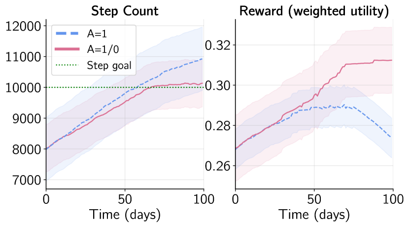
Figure 1: We compare step count and reward for two policies: one policy (blue, dashed) always sends notifications, and another policy (red, solid) sends notifications only when a user’s step count drops below their desired goal (green dashed line). A policy that always sends a notification achieves higher step count, but lower reward due to notification burden. Shaded area is $\pm 1\sigma$ across $P=20$ participants.

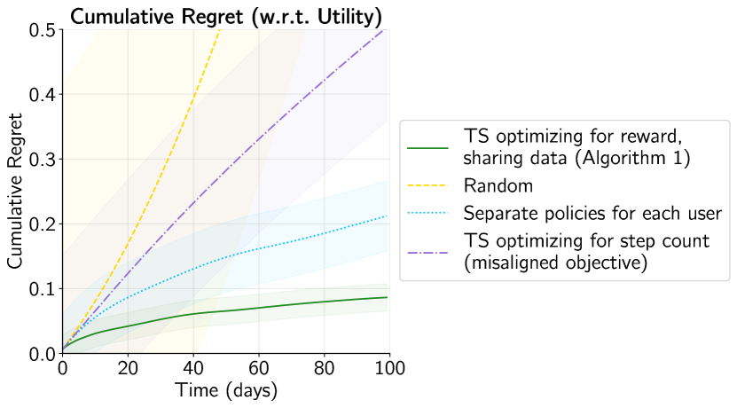
Figure 2: We compare our approach to traditional Thompson sampling optimizing for step count, a random policy, and separate policies for each user. Our approach generates less cumulative regret because it is selective about sending notifications and is optimizing for the correct element, the reward. Shaded area is $\pm 1\sigma$ across 100 trials.

We now demonstrate the results of our algorithm using a simulator inspired by mobile health intervention studies such as HeartSteps (Klasnja et al., 2018). The HeartSteps study aims to improve users’ physical activity outcomes by adaptively sending notifications encouraging them to walk. We draw inspiration from prior simulators designed to model the HeartSteps study (Yao et al., 2021; Liao et al., 2015), with some modifications specific to our setting.

First, we model treatment effect heterogeneity and non-stationarity by positing two cluster of users: active and inactive users. Empirically, studies have found that some users consistently respond positively to notifications, whereas others’ response declines over time (Liao et al., 2015). The MyHeart Counts study (Shcherbina et al., 2019), which contains a similar setup to HeartSteps without adaptive interventions, also describes clusters of users with varying baseline activity levels and treatment responses. Next, we adopt an autoregressive structure to model these individual variations. This allows for an intervention at timestep $t$ to impact future timesteps $t^{\prime}>t$ while preserving a bandit model, allowing us model habit formation (Hagger, 2019; Peng et al., 2021). Lastly, we keep track of the number of notifications that a user has received over the course of the study in order to model notification burden. Wang et al. (2021) notes that too many notifications negatively impact on a user’s engagement with the study, and we want to explicitly model the tradeoff between sending notifications and increasing step count.

To construct our simulator (described in full detail in Appendix B), we model one outcome $y_{i,t}$ (step count) as a function of $\boldsymbol{\phi}_{i,t}$, which contains information such as the previous day’s step count $y_{i,t-1}$ and group specific treatment effects. We define two utility functions $U_{i,t,0}$, a piecewise linear function that models step count goals, and $U_{i,t,1}$, which penalizes higher numbers of notifications. Inspired by habituation and recovery dynamics evidenced in prior work, we choose a quadratic function to represent notification burden (Mintz et al., 2019; Bertsimas et al., 2022). We model group differences by assuming that inactive users have a lower baseline activity level and treatment effect than active users, with individual variation resulting from the auto-regressive structure in each population. We assume that active users place a higher weight on their step count goal and a lower weight on the notification goal, and vice versa for inactive users.

Now, we evaluate our proposed algorithm in the step count simulator. We first note that optimizing for the outcome, step count, is not equivalent to optimizing for reward, which is a combination of utility functions. In Figure 2, we see that it is possible to increase step count by always sending notifications, but that this eventually reduces reward due to our notification penalty, meaning that a user would not achieve their personal goal of achieving their step count with minimal notification burden.

Next, we present results comparing four choices for algorithms: a random policy, Thompson sampling optimizing for $y_{i,t}$, Thompson sampling optimizing for $r_{i,t}$ (Algorithm 2), and one which learns indepdent policies for each user without sharing data. We find that Thompson sampling optimzing for $r_{i,t}$ generates the lowest cumulative regret across our horizon ($T=100$, $P=20$) when cumulative regret is measured with respect to reward (Eq. 3), because it can correctly balance the number of notifications sent while optimizing for a user’s goals. Additionally, we find that we get a speedup in cumulative regret when we share data, indicating that sharing data allows us to learn the optimal policy for each user more quickly.

4 Discussion

In this work, we introduce a modification to Thompson sampling that allows us to effectively optimize for user-specific goals that only introduces a constant Lipschitz penalty on cumulative regret. In simulation, we demonstrate that our approach achieves a cumulative regret speedup in comparison to policies that are trained separately for each user and policies that do not account for user-specific utilities.

There are a number of exciting directions for future work. We are actively developing semi-synthetic simulators based on empirical study data to evaluate our algorithm under more realistic conditions. This may require us to relax our linearity assumptions, e.g., using Gaussian processes (Chowdhury and Gopalan, 2017) or semi-parametric models (Greenewald et al., 2017; Krishnamurthy et al., 2018), and explicitly account for treatment effect heterogeneity, e.g., using hierarchical (Hong et al., 2022) or mixed-effects models (Tomkins et al., 2020). Moreover, our bandit model accounts for non-stationarity and habituation by including time-dependent treatment effect terms in the context and penalizing excessive notifications in the reward. While this bandit model has sample complexity benefits, it may be more appropriate to model long-term treatment effect dynamics using an MDP model, which could also be learned using Thompson sampling (Osband et al., 2013).

Towards expanding our theoretical results, our algorithm and regret bounds assume that each action is assigned sequentially (i.e., the model is updated between assigning treatment to user $i$ and $i+1$), though in practice treatment would likely be assigned in parallel. Further, it may be possible to achieve similar regret guarantees for non-Lipschitz utility functions, e.g., indicator functions with a fininte number of discontinuities. It may also prove useful to derive simple regret bounds to investigate whether the presence of user-specific goals can change exploration strategies in a pure exploration setting.

We thank Jonathan Lee, Jiayu Yao, and Scott Fleming for feedback. AM was supported in part by a Stanford Engineering Fellowship. This work was supported in part by NSF grant #2112926.

Appendix A Bayesian Regret Proof

The proof structure largely follows Lattimore and Szepesvári (2020) Theorem 36.4, with modifications to account for our Lipschitz utility transformations.

Theorem 1

After running Algorithm 2 for $N=P\cdot T$ samples, where $P$ is the number of participants in the cohort and $T$ is the time horizon, we achieves Bayesian cumulative regret on the order of

$$\text{BR}(N)\leq O(Ld\sqrt{N\log(NM)\log(N/d)})$$

Proof: For simplicity, we define $n=Pt+i$ to convert the nested index $(i,t)$ to a single index. Using this notation, recall that

$$r_{n}(s,a) =\sum_{k=1}^{K}w_{n,k}\cdot U_{n,k}\Big{(}[\mathbf{y}(s,a)]_{m_{k}},\boldsymbol{\phi}(s,a)\Big{)},\quad\text{where }[\mathbf{y}(s,a)]_{m}=\boldsymbol{\theta}_{m}^{\top}\boldsymbol{\phi}(s,a)+\varepsilon,\quad\sum_{k=1}^{K}w_{n,k}=1$$ (5)

Writing $y_{n,m}\triangleq[\mathbf{y}(s_{n},a_{n})]_{m}$ and $\boldsymbol{\phi}_{n}\triangleq\boldsymbol{\phi}(s_{n},a_{n})$, define

$$\hat{\boldsymbol{\theta}}_{n,m} =\Sigma_{n}^{-1}\Phi_{n}^{\top}Y_{n,m},\quad\Phi_{n}=\begin{bmatrix}\rule[2.15277pt]{10.76385pt}{0.5pt}&\boldsymbol{\phi}_{1}^{\top}&\rule[2.15277pt]{10.76385pt}{0.5pt}\\ &\vdots&\\ \rule[2.15277pt]{10.76385pt}{0.5pt}&\boldsymbol{\phi}_{n}^{\top}&\rule[2.15277pt]{10.76385pt}{0.5pt}\\ \end{bmatrix},\quad Y_{n,m}=\begin{bmatrix}y_{1,m}\\ \vdots\\ y_{n,m}\end{bmatrix},\quad\Sigma_{n}=\Phi_{n}^{\top}\Phi_{n}+\lambda I_{d}$$ (6)

Assume that $\forall m,\|\boldsymbol{\theta}_{m}\|_{2}\leq S$, $\sup_{s,a}\|\boldsymbol{\phi}(s,a)\|_{2}\leq Q$, $\forall m,\sup_{s,a}|\boldsymbol{\theta}_{m}^{\top}\boldsymbol{\phi}(s,a)|\leq 1$. Let each $U_{n,k}$ be $L$-Lipschitz in $y$: $|U(y,\boldsymbol{\phi})-U(y^{\prime},\boldsymbol{\phi})|\leq L|y-y^{\prime}|$. Define the upper confidence bound

$$\text{UCB}_{n}(s,a) =\sum_{k=1}^{K}w_{n,k}\cdot U_{n,k}\Big{(}\hat{y}_{n,m_{k}}(s,a),\boldsymbol{\phi}(s,a)\Big{)}+\beta L\|\boldsymbol{\phi}(s,a)\|_{\Sigma_{n-1}^{-1}}$$ (7)

$$\hat{y}_{n,m}(s,a) =\boldsymbol{\phi}(s,a)^{\top}\hat{\boldsymbol{\theta}}_{n-1,m}$$ (8)

$$\beta =\sqrt{\lambda}S+\sqrt{2\log\left(NM\right)+d\log\left(1+\frac{NQ^{2}}{\lambda d}\right)}$$ (9)

By Lattimore and Szepesvári (2020) Theorem 20.5 and a union bound over $m\in[M]$, it holds that

$$P\left(\exists m,\exists n\leq N:\|\hat{\boldsymbol{\theta}}_{n-1,m}-\boldsymbol{\theta}_{m}\|_{\Sigma_{n-1}}\geq\beta\right)\leq\frac{1}{N}$$ (10)

Let $E_{n}$ denote the event that $\forall m,\|\hat{\boldsymbol{\theta}}_{n-1,m}-\boldsymbol{\theta}_{m}\|_{\Sigma_{n-1}}\leq\beta$ and let $E=\bigcap_{n=1}^{N}E_{n}$. Define $H_{n}=\{(\boldsymbol{\phi}_{n^{\prime}},\mathbf{y}_{n^{\prime}})\}_{n^{\prime}=1}^{n}$ to be the history up until time $n$. We have that

$$\text{BR}(N) =\mathbb{E}\left[\sum_{n=1}^{N}r_{n}(s_{n},a_{s_{n}}^{*})-r_{n}(s_{n},a_{n})\right]$$ (11)

$$=\mathbb{E}\left[\mathbbm{1}\{E^{c}\}\sum_{n=1}^{N}r_{n}(s_{n},a_{s_{n}}^{*})-r_{n}(s_{n},a_{n})\right]+\mathbb{E}\left[\mathbbm{1}\{E\}\sum_{n=1}^{N}r_{n}(s_{n},a_{s_{n}}^{*})-r_{n}(s_{n},a_{n})\right]$$ (12)

$$=2LN\cdot\mathbb{E}\left[\mathbbm{1}\{E^{c}\}\right]+\mathbb{E}\left[\mathbbm{1}\{E\}\sum_{n=1}^{N}r_{n}(s_{n},a_{s_{n}}^{*})-r_{n}(s_{n},a_{n})\right]$$ (13)

$$\leq 2L+\mathbb{E}\left[\sum_{n=1}^{N}\mathbb{E}\Big{[}\mathbbm{1}\{E_{n}\}\left(r_{n}(s_{n},a_{s_{n}}^{*})-r_{n}(s_{n},a_{n})\right)\ |\ H_{n-1}\Big{]}\right]$$ (14)

Note that the first term in Eq. 12 is bounded by $2LN$ since $|r_{n}(s,a)-r_{n}(s^{\prime},a^{\prime})|\leq L\sum_{k}w_{n,k}|y_{m_{k}}(s,a)-y_{m_{k}}(s^{\prime},a^{\prime})|\leq 2L$.

Define $a_{s_{n}}^{\star}=\mathop{\mathrm{arg\,max}}_{a}r_{n}(s_{n},a)$ to be the optimal action in state $s_{n}$. Noting that $P(a_{s_{n}}^{\star}=\cdot|H_{n})=P(a_{n}=\cdot|H_{n})$, we have that

$$\mathbb{E}\left[\mathbbm{1}\{E_{n}\}\Big{(}r_{n}(s_{n},a_{s_{n}}^{*})-r_{n}(s_{n},a_{n})\Big{)}\ |\ H_{n-1}\right]$$ (15)

$$=\mathbb{E}\left[\mathbbm{1}\{E_{n}\}\Big{(}r_{n}(s_{n},a_{s_{n}}^{*})-\text{UCB}_{n}(s_{n},a_{n})+\text{UCB}_{n}(s_{n},a_{n})-r_{n}(s_{n},a_{n})\Big{)}\ |\ H_{n-1}\right]$$ (16)

$$=\mathbb{E}\left[\mathbbm{1}\{E_{n}\}\Big{(}r_{n}(s_{n},a_{s_{n}}^{*})-\text{UCB}_{n}(s_{n},a_{s_{n}}^{*})+\text{UCB}_{n}(s_{n},a_{n})-r_{n}(s_{n},a_{n})\Big{)}\ |\ H_{n-1}\right]$$ (17)

$$\leq\mathbb{E}\left[\mathbbm{1}\{E_{n}\}\Big{(}\text{UCB}_{n}(s_{n},a_{n})-r_{n}(s_{n},a_{n})\Big{)}\ |\ H_{n-1}\right]$$ (18)

The inequality in Eq. 18 follows from the fact that $\text{UCB}_{n}(s,a)\geq r_{n}(s,a)$ given $E_{n}$. Continuing, we find that

$$\mathbb{E}\left[\mathbbm{1}\{E_{n}\}\Big{(}\text{UCB}_{n}(s_{n},a_{n})-r_{n}(s_{n},a_{n})\Big{)}\ |\ H_{n-1}\right]$$ (19)

$$\leq\mathbb{E}\left[\mathbbm{1}\{E_{n}\}\left(\sum_{k=1}^{K}w_{n,k}\left(U_{n,k}(\hat{y}_{n,m_{k}},\boldsymbol{\phi}_{n})-U_{n,k}(y_{n,m_{k}},\boldsymbol{\phi}_{n})\right)+\beta L\|\boldsymbol{\phi}_{n}\|_{\Sigma_{n-1}^{-1}}\right)\ |\ H_{n-1}\right]$$ (20)

$$\leq\mathbb{E}\left[\mathbbm{1}\{E_{n}\}\left(\sum_{k=1}^{K}w_{n,k}L|\hat{y}_{n,m_{k}}-y_{n,m_{k}}|+\beta L\|\boldsymbol{\phi}_{n}\|_{\Sigma_{n-1}^{-1}}\right)\ |\ H_{n-1}\right]$$ (21)

$$=\mathbb{E}\left[\mathbbm{1}\{E_{n}\}\left(\sum_{k=1}^{K}w_{n,k}L|\langle\boldsymbol{\phi}_{n},\hat{\boldsymbol{\theta}}_{n-1,m_{k}}-\boldsymbol{\theta}_{m_{k}}\rangle|+\beta L\|\boldsymbol{\phi}_{n}\|_{\Sigma_{n-1}^{-1}}\right)\ |\ H_{n-1}\right]$$ (22)

$$\leq\mathbb{E}\left[\mathbbm{1}\{E_{n}\}\left(\sum_{k=1}^{K}w_{n,k}L\|\boldsymbol{\phi}_{n}\|_{\Sigma_{n-1}^{-1}}\|\hat{\boldsymbol{\theta}}_{n-1,m_{k}}-\boldsymbol{\theta}_{m_{k}}\|_{\Sigma_{n-1}}+\beta L\|\boldsymbol{\phi}_{n}\|_{\Sigma_{n-1}^{-1}}\right)\ |\ H_{n-1}\right]$$ (23)

$$\leq\mathbb{E}\left[2L\beta\|\boldsymbol{\phi}_{n}\|_{\Sigma_{n-1}^{-1}}\ |\ H_{n-1}\right]$$ (24)

Plugging the above into Eq. 14 combined with $\mathbb{E}\left[r_{n}(s_{n},a_{s_{n}}^{*})-r_{n}(s_{n},a_{n})\right]\leq 2L$, we conclude that

$$\text{BR}(N) \leq 2L+2L\beta\cdot\mathbb{E}\left[\sum_{n=1}^{N}\min\left(1,\|\boldsymbol{\phi}_{n}\|_{\Sigma_{n-1}^{-1}}\right)\right]$$ (25)

$$\leq 2L+2L\beta\cdot\sqrt{N\cdot\mathbb{E}\left[\sum_{n=1}^{N}\min\left(1,\|\boldsymbol{\phi}_{n}\|_{\Sigma_{n-1}^{-1}}^{2}\right)\right]}$$ (26)

$$\leq 2L+2L\beta\cdot\sqrt{2Nd\log\left(1+\frac{NQ^{2}}{\lambda d}\right)}$$ (27)

$$=2L\left(1+\left(\sqrt{\lambda}S+\sqrt{2\log\left(NM\right)+d\log\left(1+\frac{NQ^{2}}{\lambda d}\right)}\right)\sqrt{2Nd\log\left(1+\frac{NQ^{2}}{\lambda d}\right)}\right)$$ (28)

Eq. 26 follows from Cauchy-Schwarz and Eq. 27 follows from the elliptical potential lemma (Lattimore and Szepesvári (2020) Lemma 19.4).

In conclusion, under the assumption that $Q,S,\lambda$ are $O(1)$, we have that the Bayesian regret is of order $O(Ld\sqrt{N\log(NM)\log(N/d)})$

Appendix B Step Count Simulator

Here we discuss the details of the simulator. We model one outcome $(M=1)$, step count, and assume the step count outcome follows a linear model,

$$y_{i,t}=\boldsymbol{\phi}_{i,t}^{\top}\boldsymbol{\theta}^{\star}+\varepsilon$$ (29)

where $\varepsilon\sim\mathcal{N}(0,0.15^{2})$. The featurization $\boldsymbol{\phi}_{i,t}=[1,y_{i,t-1},t_{a},t_{i},nn]$ contains two components that represent the treatment effect for each of the two groups ($t_{a}$ for active users and $t_{i}$ for inactive users) and one counter that accumulates the number of notifications ($nn$). The treatment effect is represented as a decaying sigmoid of the number of notifications. For the active group it is

$$t_{a}(nn)=1-\sigma\left(\left(nn-\frac{T}{1.9}\right)\cdot\frac{10}{T}\right)$$ (30)

and for the inactive group it is

$$t_{i}(nn)=1-\sigma\left(\left(nn-\frac{T}{1.3}\right)\cdot\frac{4}{T}\right)$$ (31)

We set $\boldsymbol{\theta}^{\star}=[-0.02,0.999,0.3,0.21,0]$, which ignores the number of notifications that have been sent to a user.

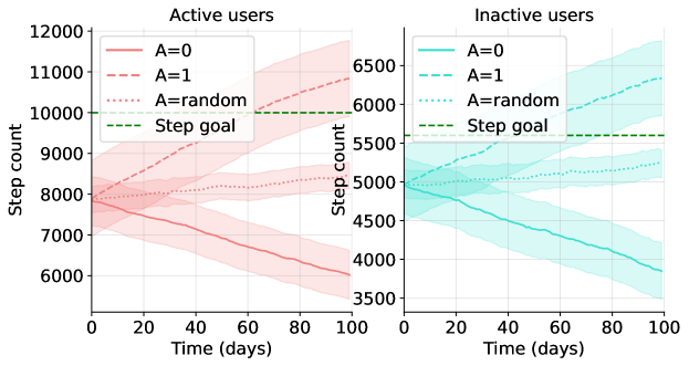
Figure 3: Comparing treatment effect between active and inactive groups.

The first utility function upweights step count and is given by

$$U_{i,t,0}(y_{i,t},\boldsymbol{\phi}_{i,t})=\begin{cases}\alpha_{1}\cdot y_{i,t}&y_{i,t}\leq\text{step goal}\\ \alpha_{2}\cdot y_{i,t}+\gamma&y_{i,t}>\text{step goal}\end{cases}$$ (32)

where $\alpha_{1}=0.005,\alpha_{2}=0.001$, $\gamma=0.42$ if the user is an active user, and $\gamma=0.3$ if the user is an inactive user. The step count goal for active users is $10,000$ steps, and for inactive users it is $5,600$ steps. This utility is a piecewise linear function with a high slope before a user achieves their step count goal, and a much smaller slope afterwards. The second utility function is given by

$$U_{i,t,1}(y_{i,t},\boldsymbol{\phi}_{i,t})=-\beta((nn)^{2})$$ (33)

where $\beta=0.00003$. This utility decreases quadratically as the number of notifications increases.

References

- Agrawal and Goyal (2013) Shipra Agrawal and Navin Goyal. Thompson sampling for contextual bandits with linear payoffs. In International conference on machine learning, pages 127–135. PMLR, 2013.
- Baek et al. (2023) Jackie Baek, Justin J. Boutilier, Vivek F. Farias, Jonas Oddur Jonasson, and Erez Yoeli. Policy optimization for personalized interventions in behavioral health, 2023.
- Bertsimas et al. (2022) Dimitris Bertsimas, Predrag Klasnja, Susan Murphy, and Liangyuan Na. Data-driven interpretable policy construction for personalized mobile health. In 2022 IEEE International Conference on Digital Health (ICDH), pages 13–22, 2022. 10.1109/ICDH55609.2022.00010.
- Chowdhury and Gopalan (2017) Sayak Ray Chowdhury and Aditya Gopalan. On kernelized multi-armed bandits. In International Conference on Machine Learning, pages 844–853. PMLR, 2017.
- Domin et al. (2021) Alex Domin, Donna Spruijt-Metz, Daniel Theisen, Yacine Ouzzahra, Claus Vögele, et al. Smartphone-based interventions for physical activity promotion: scoping review of the evidence over the last 10 years. JMIR mHealth and uHealth, 9(7):e24308, 2021.
- Ekhtiar et al. (2023) Tina Ekhtiar, Armağan Karahanoğlu, Rúben Gouveia, and Geke Ludden. Goals for goal setting: A scoping review on personal informatics. 2023.
- Epton et al. (2017) Tracy Epton, Sinead Currie, and Christopher J Armitage. Unique effects of setting goals on behavior change: Systematic review and meta-analysis. Journal of consulting and clinical psychology, 85(12):1182, 2017.
- Greenewald et al. (2017) Kristjan Greenewald, Ambuj Tewari, Susan Murphy, and Predag Klasnja. Action centered contextual bandits. Advances in neural information processing systems, 30, 2017.
- Hagger (2019) Martin S Hagger. Habit and physical activity: Theoretical advances, practical implications, and agenda for future research. Psychology of Sport and Exercise, 42:118–129, 2019.
- Hariri et al. (2015) Negar Hariri, Bamshad Mobasher, and R. Burke. Adapting to user preference changes in interactive recommendation. In International Joint Conference on Artificial Intelligence, 2015.
- Hicks et al. (2023) Jennifer L Hicks, Melissa A Boswell, Tim Althoff, Alia J Crum, Joy P Ku, James A Landay, Paula ML Moya, Elizabeth L Murnane, Michael P Snyder, Abby C King, et al. Leveraging mobile technology for public health promotion: A multidisciplinary perspective. Annual Review of Public Health, 44:131–150, 2023.
- Hong et al. (2022) Joey Hong, Branislav Kveton, Manzil Zaheer, and Mohammad Ghavamzadeh. Hierarchical bayesian bandits, 2022.
- Howlett et al. (2019) Neil Howlett, Daksha Trivedi, Nicholas A Troop, and Angel Marie Chater. Are physical activity interventions for healthy inactive adults effective in promoting behavior change and maintenance, and which behavior change techniques are effective? a systematic review and meta-analysis. Translational behavioral medicine, 9(1):147–157, 2019.
- Klasnja et al. (2018) Predrag Klasnja, Shawna Smith, Nicholas Seewald, Andy Jinseok Lee, Kelly Hall, Brook Luers, Eric Hekler, and Susan Murphy. Efficacy of contextually tailored suggestions for physical activity: A micro-randomized optimization trial of heartsteps. Annals of Behavioral Medicine, 53, 09 2018. 10.1093/abm/kay067.
- Klasnja et al. (2019) Predrag Klasnja, Shawna Smith, Nicholas J Seewald, Andy Lee, Kelly Hall, Brook Luers, Eric B Hekler, and Susan A Murphy. Efficacy of contextually tailored suggestions for physical activity: a micro-randomized optimization trial of heartsteps. Annals of Behavioral Medicine, 53(6):573–582, 2019.
- Krishnamurthy et al. (2018) Akshay Krishnamurthy, Zhiwei Steven Wu, and Vasilis Syrgkanis. Semiparametric contextual bandits. In International Conference on Machine Learning, pages 2776–2785. PMLR, 2018.
- Lattimore and Szepesvári (2020) Tor Lattimore and Csaba Szepesvári. Bandit algorithms. Cambridge University Press, 2020.
- Liao et al. (2015) Peng Liao, Predrag Klasnja, Ambuj Tewari, and Susan Murphy. Sample size calculations for micro-randomized trials in mhealth. Statistics in medicine, 35, 12 2015. 10.1002/sim.6847.
- Locke and Latham (2002) Edwin A Locke and Gary P Latham. Building a practically useful theory of goal setting and task motivation: A 35-year odyssey. American psychologist, 57(9):705, 2002.
- McEwan et al. (2016) Desmond McEwan, Samantha M Harden, Bruno D Zumbo, Benjamin D Sylvester, Megan Kaulius, Geralyn R Ruissen, A Justine Dowd, and Mark R Beauchamp. The effectiveness of multi-component goal setting interventions for changing physical activity behaviour: a systematic review and meta-analysis. Health psychology review, 10(1):67–88, 2016.
- Mintz et al. (2019) Yonatan Mintz, Anil Aswani, Philip Kaminsky, Elena Flowers, and Yoshimi Fukuoka. Non-stationary bandits with habituation and recovery dynamics, 2019.
- Olsen and Nesbitt (2010) Jeanette M Olsen and Bonnie J Nesbitt. Health coaching to improve healthy lifestyle behaviors: an integrative review. American journal of health promotion, 25(1):e1–e12, 2010.
- Osband et al. (2013) Ian Osband, Daniel Russo, and Benjamin Van Roy. (more) efficient reinforcement learning via posterior sampling. Advances in Neural Information Processing Systems, 26, 2013.
- Peng et al. (2021) Wei Peng, Lin Li, Anastasia Kononova, Shelia Cotten, Kendra Kamp, Marie Bowen, et al. Habit formation in wearable activity tracker use among older adults: qualitative study. JMIR mHealth and uHealth, 9(1):e22488, 2021.
- Roijers et al. (2021) Diederik Roijers, Luisa Zintgraf, Pieter Libin, Mathieu Reymond, Eugenio Bargiacchi, and Ann Nowe. Interactive Multi-objective Reinforcement Learning in Multi-armed Bandits with Gaussian Process Utility Models, pages 463–478. 02 2021. ISBN 978-3-030-67663-6. 10.1007/978-3-030-67664-3_28.
- Ruggeri et al. (2023) Kai Ruggeri, Amel Benzerga, Sanne Verra, and Tomas Folke. A behavioral approach to personalizing public health. Behavioural Public Policy, 7(2):457–469, 2023. 10.1017/bpp.2020.31.
- Shcherbina et al. (2019) Anna Shcherbina, Steven G Hershman, Laura Lazzeroni, Abby C King, Jack W O’Sullivan, Eric Hekler, Yasbanoo Moayedi, Aleksandra Pavlovic, Daryl Waggott, Abhinav Sharma, Alan Yeung, Jeffrey W Christle, Matthew T Wheeler, Michael V McConnell, Robert A Harrington, and Euan A Ashley. The effect of digital physical activity interventions on daily step count: a randomised controlled crossover substudy of the myheart counts cardiovascular health study. The Lancet Digital Health, 1(7):e344–e352, 2019. ISSN 2589-7500. https://doi.org/10.1016/S2589-7500(19)30129-3.
- Tomkins et al. (2020) Sabina Tomkins, Peng Liao, Predrag Klasnja, and Susan Murphy. Intelligentpooling: Practical thompson sampling for mhealth, 2020.
- Wang et al. (2021) Shihan Wang, Chao Zhang, Ben Kröse, and Herke Hoof. Optimizing adaptive notifications in mobile health interventions systems: Reinforcement learning from a data-driven behavioral simulator. Journal of Medical Systems, 45, 12 2021. 10.1007/s10916-021-01773-0.
- Wolever et al. (2013) Ruth Q Wolever, Leigh Ann Simmons, Gary A Sforzo, Diana Dill, Miranda Kaye, Elizabeth M Bechard, Mary Elaine Southard, Mary Kennedy, Justine Vosloo, and Nancy Yang. A systematic review of the literature on health and wellness coaching: defining a key behavioral intervention in healthcare. Global advances in health and medicine, 2(4):38–57, 2013.
- World Health Organization (2022) World Health Organization. Physical activity, 2022. URL https://www.who.int/en/news-room/fact-sheets/detail/physical-activity.
- Yang and Van Stee (2019) Qinghua Yang and Stephanie K Van Stee. The comparative effectiveness of mobile phone interventions in improving health outcomes: meta-analytic review. JMIR mHealth and uHealth, 7(4):e11244, 2019.
- Yang et al. (2020) Xiaotian Yang, Lin Ma, Xi Zhao, and Atreyi Kankanhalli. Factors influencing user’s adherence to physical activity applications: A scoping literature review and future directions. International Journal of Medical Informatics, 134:104039, 2020.
- Yao et al. (2021) Jiayu Yao, Emma Brunskill, Weiwei Pan, Susan Murphy, and Finale Doshi-Velez. Power constrained bandits. In Proceedings of the 6th Machine Learning for Healthcare Conference, pages 209–259, 2021.
- Zhou and Brunskill (2016) Li Zhou and Emma Brunskill. Latent contextual bandits and their application to personalized recommendations for new users. In Proceedings of the Twenty-Fifth International Joint Conference on Artificial Intelligence, pages 3646–3653, 2016.