Show Your Work with Confidence:
Confidence Bands for Tuning Curves

Abstract

The choice of hyperparameters greatly impacts performance in natural language processing. Often, it is hard to tell if a method is better than another or just better tuned. Tuning curves fix this ambiguity by accounting for tuning effort. Specifically, they plot validation performance as a function of the number of hyperparameter choices tried so far. While several estimators exist for these curves, it is common to use point estimates, which we show fail silently and give contradictory results when given too little data.

Beyond point estimates, confidence bands are necessary to rigorously establish the relationship between different approaches. We present the first method to construct valid confidence bands for tuning curves. The bands are exact, simultaneous, and distribution-free, thus they provide a robust basis for comparing methods.

Empirical analysis shows that while bootstrap confidence bands, which serve as a baseline, fail to approximate their target confidence, ours achieve it exactly. We validate our design with ablations, analyze the effect of sample size, and provide guidance on comparing models with our method. To promote confident comparisons in future work, we release a library implementing the method: https://github.com/nalourie/opda.

Show Your Work with Confidence:
Confidence Bands for Tuning Curves

Nicholas Lourie New York University nick.lourie@nyu.edu                        Kyunghyun Cho New York University & Genentech kyunghyun.cho@nyu.edu                        He He New York University hhe@nyu.edu

1 Introduction

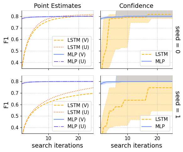
Figure 1: The charts compare tuning curves for MLP and LSTM text classifiers on Reuters (Apté et al., 1994), based on data from Tang et al. (2020). The tuning curve plots the F1 score of the best model after each round of random search. The left compares point estimates for the mean based on U and V-statistics; the right compares 50% confidence bands for the median tuning curve. The top and the bottom run the same analysis on different samples of 25 search iterations. The point estimates give contradictory conclusions without warning on different samples, disagreeing whether the LSTM ever beats the MLP. The differences between estimators are small in comparison to this sample variation. Confidence bands, in contrast, directly show the variation due to sampling.

Accounting for hyperparameter tuning when comparing models is an important, open problem in NLP research. This problem is particularly relevant right now, as the rush to scale up has left us with large, costly language models and little understanding of how different designs compare. Indeed, many earlier models are now outperformed by others an order of magnitude smaller—the main difference: better hyperparameters. Even worse, the challenge of managing hyperparameters during research has produced false scientific conclusions, such as the belief that model size should scale faster than data (Hoffmann et al., 2022). As a scientific community, we require more rigorous, reliable analyses for understanding if a model is well-tuned and how costly that process is.

To tackle this issue, NLP researchers developed the tuning curve (Dodge et al., 2019; Tang et al., 2020; Dodge et al., 2021). The tuning curve plots current validation performance as a function of tuning effort, for example the total iterations or compute used in hyperparameter search (see Figure 1). By comparing tuning curves, you can determine which method is best for a given budget or judge whether the hyperparameters are fully tuned.

In theory, tuning curves solve the hyperparameter comparison problem; in practice, the curves must be estimated from data. Prior work developed efficient estimators for tuning curves (Dodge et al., 2019); however, these estimators lack corresponding methods to quantify their uncertainty. Generic techniques, such as bootstrap resampling (Efron and Tibshirani, 1994), break down for tuning curve estimates—failing to meaningfully capture their uncertainty (Tang et al., 2020). As a result, it is hard to know when a conclusion is trustworthy or whether more data is required (§5.1). This absence of confidence bands for tuning curves has hindered their more widespread adoption; and it is this gap in the existing literature we seek to fill.

To address these shortcomings, we present the first confidence bands for tuning curves to achieve meaningful coverage. Unlike the bootstrap, our bands cover the true tuning curve with precisely the prescribed probability, making them exact. Moreover, this guarantee is not asymptotic, but even holds in finite samples. The only requirement is that the scores have a continuous distribution. Thus, being free from any parametric assumptions, our bands are distribution-free and widely applicable. Lastly, they are simultaneous, i.e. contain the entire curve at once, as opposed to pointwise, or cover each point separately with the desired probability instead of all at the same time. Since the bands are simultaneous, they enable us to rigorously evaluate the model across all budgets.

Our key insight is to translate simultaneous confidence bands for the test scores’ cumulative distribution function (CDF) into confidence bands for the tuning curve, via an algebraic relationship (§3.2). Specifically, we take nonparametric bounds for the CDF, translate those to bound the CDF of the best score for a given tuning budget, then leverage that to bound a summary of the best score’s distribution (e.g., the median or the mean). Figure 2 exhibits the end result: given competing models (DeBERTa and DeBERTaV3), we account for tuning effort by comparing tuning curves, and for sample variation by reporting them with confidence bands. In this way, our confidence bands empower researchers and practitioners to confidently identify the cost regimes where one method outperforms the other.

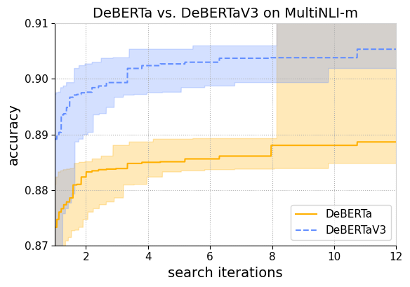
Figure 2: Median tuning curves on MultiNLI (matched) with 80% confidence, based on 48 search iterations. Point estimates plot the empirical CDFs’ tuning curves. The tuning curve is the performance of the best model as a function of the number of rounds of random search.

Complementing our theoretical analysis, we empirically study the confidence bands’ properties. Even when point estimators agree, different samples could result in different conclusions due to undetected sample variation—which the bootstrap fails to capture (§5.1). In contrast, our confidence bands attain exact coverage, both in theory and in practice, as we confirm in experiments that fine-tune pretrained models on natural language inference (§5.2). Beyond our method’s core strategy, it also incorporates several more subtle design decisions. We show how each idea contributes to tighter confidence bands through ablation studies (§5.3). Generalizing prior work, we consider median as well as mean tuning curves, and find the median provides a more interpretable, tractable, and useful point of comparison (§5.4). Finally, while confidence bands reveal sample variation, they do not eliminate it—so, we study the effect of sample size to guide how much data is necessary to estimate the tuning curve well (§5.5).

Before diving into details, we will exhibit the end result. The next section demonstrates how to use of our confidence bands in a practical scenario drawn from the literature: evaluating DeBERTaV3 (He et al., 2021a) against its baseline, DeBERTa (He et al., 2021b) (§2). Bringing it all together, this tutorial shows how tuning curves promote reliable comparisons by accounting for tuning effort, while confidence bands reveal when a method is truly better versus when more data is required to reach a conclusion. Because our confidence bands are distribution-free with exact coverage, they provide a rigorous, statistical basis for comparing methods that involve hyperparameters, sampling, or random initialization. To promote reliable comparisons and more reproducible research, we release a library implementing our method at https://github.com/nalourie/opda.

2 Tutorial: Evaluating DeBERTaV3

Let’s walk through a case study fine-tuning a pretrained model, DeBERTaV3 (He et al., 2021a), to see how our analysis works in practice.

First, we design the search distribution. Just like grid search, for each hyperparameter we choose a linear or log scale, pick upper and lower bounds, then set a (log) uniform distribution between them. For DeBERTaV3, we use a log scale for the learning rate (1e-6, 1e-3), and a linear scale for number of epochs (1, 4), batch size (16, 64), proportion of the first epoch for learning rate warmup (0, 0.6), and dropout (0, 0.3). With this distribution, we then run 48 rounds of random search.

From these samples, we construct the tuning curve and confidence bands in Figure 3. This plot quantifies the model’s performance as a function of tuning budget. From it, practitioners can tell if the model is cost effective, and researchers can judge whether it is fully tuned. We see that DeBERTaV3 has high accuracy after only 2-6 rounds of search.

Beyond absolute judgments, we need relative comparisons. Figure 2 plots DeBERTaV3 against its baseline, DeBERTa. It is tempting to require the bands have no overlap before deciding one model is better than the other; however, this rule is too conservative. Inspired by Minka (2002), we (tentatively) suggest a heuristic: evidence is weak if one band excludes the other’s point estimate, fair if each band excludes the other’s point estimate, and strong if the bands have no overlap, for a nontrivial portion of the curve. Thus, there is strong evidence DeBERTaV3 beats DeBERTa for all budgets.

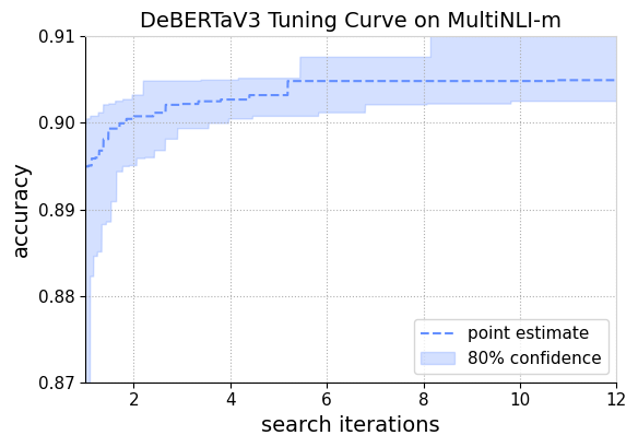
Figure 3: 80% confidence bands for the median tuning curve of DeBERTaV3 on MultiNLI (matched), using 48 samples. The point estimate is the eCDF’s tuning curve.

3 Theory

We derive confidence bands for tuning curves that are simultaneous and distribution-free. These bands are conservative for the mean tuning curve and exact for the median tuning curve when the score distribution is continuous. See §A for proofs.

3.1 Formalizing the Problem

Almost every NLP method comes with a number of hyperparameters. These hyperparameters can take any kind of value—categorical, ordinal, complex. Together, they define the hyperparameter search space, $\boldsymbol{x}=[x_{1},\ldots,x_{d}]\in\mathbb{X}$. Given a choice of hyperparameters, $\boldsymbol{x}$, evaluating the method yields a real-valued score, $y\in\mathbb{Y}\subset\mathbb{R}$, like accuracy.

Tuning algorithms search for the best possible hyperparameters by evaluating many choices. In general, the choices, $\boldsymbol{X}_{1},\ldots,\boldsymbol{X}_{n}$, and their scores, $Y_{1},\ldots,Y_{n}$, are random variables. Almost all of the search’s expense comes from training models, so the number of evaluations, $n$, is a good proxy for cost. To compare models of different sizes, this number can be multiplied by the average cost per evaluation (for example, in FLOPs). In this way, the cost-benefit trade-off between tuning effort and task performance is captured by the tuning process:

$$T_{k}\coloneqq\max_{i=1\ldots k}Y_{i}$$ (1)

or, the best performance after each evaluation.

Random search samples choices independently from a user provided search distribution, $\boldsymbol{X}_{i}\sim\mathcal{X}$. This distribution over choices induces the score distribution over the test metric: $Y_{i}\sim\mathcal{Y}$. Since every round’s score is independent and identically distributed, each $T_{k}$ is just the max from a sample of size $k$. So, if $F(y)=P(Y\leq y)$ is the CDF for $Y$, and $F_{k}(y)=P(T_{k}\leq y)$ is the CDF for $T_{k}$, then $P\left(\max_{i=1\dots k}Y_{i}\leq y\right)=P(Y\leq y)^{k}$ implies:

$$F_{k}(y)=F(y)^{k}$$ (2)

Using Equation 2, we extend the definition of $T_{k}$ to all positive real numbers $k\in\mathbb{R}_{>0}$ (rather than just natural numbers, $k\in\mathbb{N}$), by letting $T_{k}$ be the random variable with CDF $F(y)^{k}$. We can now define the expected tuning curve, $\tau_{e}(k)\coloneqq\mathbb{E}[T_{k}]$. While prior work focuses on the expected tuning curve, the median tuning curve, $\tau_{m}(k)\coloneqq\mathbb{M}[T_{k}]$, has several advantages that we will explore (§5.4).

3.2 Bounding the Tuning Curve

Our core strategy translates bounds on one round of random search into bounds on the best of $k$ rounds. §3.3 will describe how to bound one round’s CDF, $\widehat{F}^{l}(y)\leq F(y)\leq\widehat{F}^{u}(y)$, using the order statistics, $Y_{(1)},\ldots,Y_{(n)}$ (where $Y_{(i)}$ is the $i$-th least value). Equation 2 then translates these CDF bounds on $Y$ into CDF bounds on $T_{k}$:

$$(\widehat{F}^{l}(y))^{k}\leq F_{k}(y)\leq(\widehat{F}^{u}(y))^{k}$$ (3)

As our method bounds the entire CDF, it describes the full distribution of outcomes from the random search. For example, we translate the upper and lower CDF bands into lower and upper confidence bands for the mean and median tuning curves.

Mean Tuning Curve.

The confidence bands for the CDF explored in §3.3 place all probability mass on the order statistics and the bounds on $Y$. In this case, we can convert a CDF, $F_{k}$, into its expectation by summing over the order statistics and bounds weighted by their probability:

$$\hat{\tau}_{e}(k)=\sum_{i=0}^{n+1}Y_{(i)}\left[\widehat{F}\left(Y_{(i)}\right)^{k}-\widehat{F}\left(Y_{(i-1)}\right)^{k}\right]$$ (4)

where $Y_{(n+1)}$ is the upper bound on $Y$, $Y_{(0)}$ is the lower bound, and $F\left(Y_{(-1)}\right)$ is $0$ by convention. It is possible that $Y_{(n+1)}=\infty$, $Y_{(0)}=-\infty$, or both in which cases the mean could be $\infty$, $-\infty$, or undefined. If $Y$ has no finite upper bound, than the upper confidence band for the tuning curve will be vacuous, and similarly for the lower confidence band if $Y$ has no finite lower bound.

Median Tuning Curve.

In contrast, the median curve does not require finite bounds on $Y$ to yield meaningful confidence bands. We convert the CDF, $F_{k}$, into the median tuning curve directly by:

$$\hat{\tau}_{m}(k)=\min\left\{Y_{(i)}\mid 0.5\leq\widehat{F}\left(Y_{(i)}\right)^{k}\right\}$$ (5)

If $Y$ has no finite bounds, than the upper and lower confidence limits will take finite values until the bands’ endpoints, where they will diverge to $\pm\infty$. Since the CDF confidence bands are discrete, the median is generally ambiguous. Our definition takes the minimum value above at least 50% of the probability mass. This choice is motivated by the classic definition of the quantile function, $Q(p)\coloneqq\inf\{y\in\mathbb{Y}\mid p\leq F(y)\}$, which makes it a left inverse of the CDF everywhere that the distribution assigns nonzero probability mass, so $Q(F(Y))=Y$ holds with probability one.

3.3 Bounding the CDF

Our method for bounding the tuning curve (§3.2) requires simultaneous CDF bands as input. The literature offers several ways to construct these.

Given $n$ independent random variables, $Y_{i}\sim\mathcal{Y}$, we can approximate their CDF via the empirical cumulative distribution function (eCDF):

$$\widehat{F}(y)\coloneqq\frac{1}{n}\sum_{i=1}^{n}\mathbb{1}[Y_{i}\leq y]$$ (6)

This converges uniformly, almost surely to the CDF by the Glivenko-Cantelli theorem (Vaart, 1998).

DKW Bands.

The Dvoretzky-Kiefer-Wolfowitz (DKW) inequality characterizes the convergence rate (Dvoretzky et al., 1956; Massart, 1990), $\epsilon>0$:

$$P\left(\sup_{y\in\mathbb{Y}}\left|\widehat{F}(y)-F(y)\right|>\epsilon\right)\leq 2e^{-2n\epsilon^{2}}$$ (7)

In particular, the inequality bounds how far the eCDF is from the true CDF with high probability.

Setting the left to $1-\alpha$ then solving for $\epsilon$ yields simultaneous $1-\alpha$ confidence bands for the CDF:

$$\widehat{F}(y)-\epsilon\leq F(y)\leq\widehat{F}(y)+\epsilon;\hskip 5.0pt\epsilon\coloneqq\sqrt{\frac{\log\frac{2}{\alpha}}{2n}}$$ (8)

These DKW bands (and the inequality) are tight asymptotically, but conservative in finite samples.

KS Bands.

The Kolmogorov-Smirnov (KS) test tightens the DKW inequality for finite samples by taking the supremum as a test statistic:

$$D_{n}\coloneqq\sup_{y\in\mathbb{Y}}\left|\widehat{F}(y)-F(y)\right|$$ (9)

If $F$ is the true CDF and continuous, then $D_{n}$’s distribution does not depend on $Y$’s. In that case, $D_{n}$ has a (two-sided) KS distribution, and the KS test is exact and distribution-free (Bradley, 1968). We can invert it to construct simultaneous, exact, and distribution-free confidence bands for the CDF.

The DKW inequality and KS test are central tools in nonparametric statistics. The first offers a simple, closed-form formula, while the second is tighter, quick to compute, and widely implemented in software. Still, both methods share a major shortcoming: because the bands have constant width over the CDF, they are violated more often near the median. As a result, they are wider than necessary–especially at the extremes, which impact the tuning curve the most as that is where the max is.

LD Bands.

To fix this issue, Learned-Miller and DeStefano (2008) derived simultaneous confidence bands that are violated equally often at all points, and thus much narrower at the extremes. The bands are based on order statistics, $Y_{(1)},\ldots,Y_{(n)}$, where $Y_{(i)}$ is the $i$-th smallest number. If $F$ is the CDF of a continuous distribution, then $F(Y)$ is uniform from $0$ to $1$. $F\left(Y_{(i)}\right)$ is distributed as the uniform’s $i$-th order statistic, $\text{Beta}(i,n{+}1{-}i)$. Any interval containing $1-\alpha^{\prime}$ of the Beta distribution’s mass gives a $1-\alpha^{\prime}$ confidence interval for the CDF at $Y_{(i)}$: $l_{(i)}\leq F\left(Y_{(i)}\right)\leq u_{(i)}$. The Learned-Miller-DeStefano (LD) bands set $\alpha^{\prime}$ so that these pointwise intervals hold simultaneously with probability $1-\alpha$. Because the CDF is monotonic, the lower bound on $F\left(Y_{(i)}\right)$ extends to the right and the upper bound on $F\left(Y_{(i)}\right)$ extends to the left. Formally, $Y_{(i)}<y$ implies $l_{(i)}\leq F(y)$ and $y<Y_{(i)}$ implies $F(y)\leq u_{(i)}$. In this way, the confidence intervals at the order statistics bound the entire CDF.

The LD bands are not widely implemented. Learned-Miller and DeStefano (2008) adjust $\alpha^{\prime}$ (e.g., using binary search) until the correct level for $\alpha$ is obtained in simulations that estimate the coverage. This approach is very time consuming, since each iteration constructs the confidence bands thousands of times. Instead, we reformulate the confidence bands as a hypothesis test and directly simulate the test statistic’s null distribution.

Specifically, we define the test statistic:

$$L_{n}\coloneqq\max_{i=1\ldots n}B_{i}\left(F\left(Y_{(i)}\right)\right)$$ (10)

where $B_{i}(p)$ is the coverage under $\text{Beta}(i,n{+}1{-}i)$ of the smallest interval containing $p$. In general, you could consider different types of intervals. The highest probability density interval produces the best confidence bounds (§5.3), though the equal-tailed interval is easier to compute. If $\mathcal{Y}$ is a continuous distribution, then $F\left(Y_{(i)}\right)$ is uniformly distributed between $0$ and $1$ and $L_{n}$ always has the same distribution. We compute significance levels by simulating this distribution with the uniform.

Given this test, we invert it to create confidence bands: First, find the $1-\alpha$ quantile for $L_{n}$, next use it to create confidence intervals for each $F\left(Y_{(i)}\right)$, and finally extend these intervals via monotonicity, as before. This approach requires only one round of simulation, rather than one for each step of a binary search—leading to a substantial speed up.

4 Experimental Setup

Our experiments address two kinds of questions:

Comparisons to Prior Work.

We adapt data from Tang et al. (2020), who identified many of the challenges inspiring our work. The data consists of 145 and 152 rounds of random search for MLP and LSTM classifiers’ F1 scores on the Reuters document classification dataset (Apté et al., 1994). The hyperparameter search included learning rate, batch size, and dropout among others. Like Tang et al. (2020), we measure the empirical coverage of bootstrap confidence bands in simulation. We fit kernel density estimates (KDE) to MLP and LSTM hyperparameter tuning data, to simulate random search while also being able to compute the true tuning curve in this simulation. We improve Tang et al.’s (2020) protocol by using a KDE method that includes a boundary correction, to account for F1 being bounded by 0 and 1. See §B.1 for details.

Analysis in a Realistic Scenario

In addition to the experiments above, we demonstrate our tool on a practical problem from the recent literature: comparing DeBERTaV3 (He et al., 2021a) to its baseline, DeBERTa (He et al., 2021b). Using the original implementation, we trained DeBERTa and DeBERTaV3 on MultiNLI (Williams et al., 2018) evaluated with accuracy over 1,024 rounds of random search. We tuned the dropout, learning rate, batch size, number of epochs, and warmup proportion of the first epoch for both models. Moreover, we fit a KDE model to this data for our exact coverage analysis (§5.2). See §B.2 for more details.

5 Analysis

We validate our theory with empirical results.

5.1 Comparisons to Existing Methods

Prior work raises an important issue with current tuning curve estimators: such point estimates silently produce incorrect conclusions when given too little data (Tang et al., 2020; Dodge et al., 2021). Confidence bands could resolve this issue by warning when more data is required; however, bootstrap confidence bands fail to achieve meaningful coverage (Tang et al., 2020). In contrast, our confidence bands come with strong theoretical guarantees. The following experiments demonstrate how they address these issues in practice.

Point Estimators’ Drawbacks.

Experimental conclusions should not depend on the choice of estimator. Thus, if two estimators would disagree, the experiment should be redesigned—for example, with a larger sample size. Figure 1 exemplifies such a situation. The V-statistic estimator (Dodge et al., 2019) and U-statistic estimator (Tang et al., 2020) disagree (top left): the first suggests the LSTM outperforms after 20 steps, while the latter points to 13. Worse, the same analysis run on a different sample leads to a completely different conclusion (bottom left): the LSTM never beats the MLP at all. Confidence bands explain this disagreement (right): there is simply not enough data for a conclusion. So, while point estimators fail silently, confidence bands reveal issues in the experimental design.

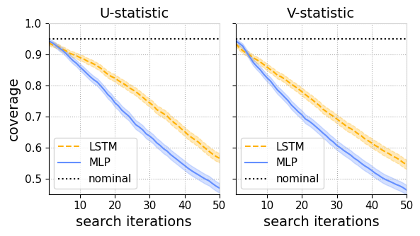
Figure 4: The pointwise coverage of 95% bootstrap confidence bands constructed from 50 search iterations. The graphs show the coverage at each point of the tuning curve, measured in simulation. The shaded regions are 95% Clopper-Pearson confidence intervals.

Shortcomings of the Bootstrap.

Bootstrapping is often an easy way to construct confidence bands (Efron and Tibshirani, 1994); unfortunately, it fails for tuning curves. While the bootstrap works under mild assumptions, Tang et al. (2020) showed these assumptions are not satisfied in practice for tuning curves. Figure 4 reproduces and expands this result, showing it for the U as well as V-statistic estimator. The X-axis fixes a point on the tuning curve, while the Y-axis is the (empirical) coverage, or percent of the time bootstrap confidence bands contained that point on the tuning curve in simulations. Near the curve’s start, the bands get close to the desired coverage, but the true coverage plummets as search iterations increase. The bootstrap is not directly comparable to our confidence bands, as we aim for simultaneous instead of pointwise coverage; still, we will see in §5.2 that our bands attain their guarantee at exactly the specified level of coverage.

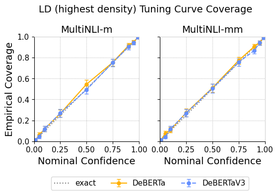
Figure 5: Nominal vs. empirical coverage of the LD median tuning curve confidence bands. Error bars show 99% Clopper-Pearson confidence intervals. The results lie on the $y=x$ line, indicating exact coverage.

5.2 Exact Coverage

To test our theory, we measure the confidence bands’ coverage empirically. Adapting the protocol from Tang et al. (2020), first we build a realistic simulation of the score distribution in which we know the true tuning curve, then we measure how often the confidence bands cover the tuning curve over many trials. To fit the simulation, we run 1,024 rounds of random search on DeBERTa and DeBERTaV3, then fit a KDE to this sample (as described in §4). Finally, we run the simulation 1,024 times, construct the confidence bands for each run, and estimate the coverage as the percentage of times the confidence bands contained the tuning curve.

Figure 5 summarizes results from our simulation study. As theory predicts, the LD bands achieve exact coverage for the median tuning curve across models and test sets. See §D for additional results.

5.3 Ablations

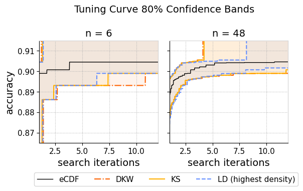
Figure 6: The DKW, KS, and LD confidence bands for DeBERTaV3’s tuning curve on MultiNLI (matched).

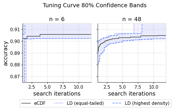
Figure 7: Equal-tailed and highest density LD bands for DeBERTaV3’s tuning curve on MultiNLI (matched).

Our basic strategy converts any simultaneous CDF bands into bounds on the tuning curve. The tuning curve bands’ tightness depends heavily on the CDF bands’ shape. Thus, the choice of CDF bands is an important design decision. Our recommended choice, the highest density LD bands, gives a tighter bound over a greater range than the alternatives.

DKW vs. KS vs. LD Bands.

We recommend the LD bands over the DKW and KS bands (§3.3). While the DKW and KS bands are much better known, both are loose at the extremes due to their constant width over the CDF. In contrast, the LD bands narrow at the extremes, leading to much tighter bounds on the tuning curve for all but the smallest sample sizes. Figure 7 confirms this hypothesis by comparing the DKW, KS, and LD bands for DeBERTaV3 on MultiNLI. For both small (6) and large (48) samples, the LD bands offer tighter bounds over the majority of the curve.

Equal-tailed vs. Highest Density Bands.

While Learned-Miller and DeStefano (2008) originally constructed CDF bands from equal-tailed intervals, we recommend highest probability density intervals instead. Highest density intervals are more costly to compute, but also yield narrower CDF bands. The narrower CDF bands translate to better tuning curve bands, as shown in Figure 7. In it, we see highest density and equal-tailed LD bands for the tuning curve of DeBERTaV3 on MultiNLI, based on small (6) and large (48) samples. Both bands have similar lower bounds; however, the highest density bands extend further right along the curve, bounding it over a greater range. This effect is even more pronounced on the larger sample.

5.4 Mean vs. Median Tuning Curves

While prior work focuses on the expected tuning curve, the median, $\mathbb{M}[T_{k}]$, has several advantages. First, the mean is difficult to interpret since $T_{k}$ can have a skewed distribution and we typically do not average over many searches. Interpreting the median, in contrast, is simple and straightforward: half the time you do better, half the time you do worse. Next, it is impossible to construct a nonparametric confidence interval for the mean unless $T_{k}$ is globally bounded, since otherwise there could be an arbitrarily small probability on an arbitrarily large number. Finally, even with global bounds, this issue causes the confidence bands for the mean to converge more slowly than those for the median, as shown in Figure 8: the median bands converge quickly on the initial part of the curve, while the bands for the mean remain loose. These reasons lead us to recommend the median over the mean.

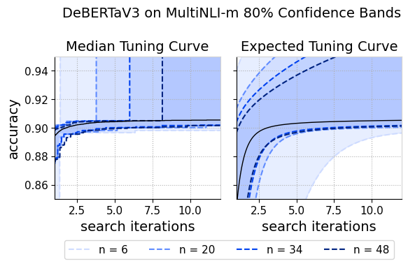
Figure 8: Confidence bands for the median vs. mean.

5.5 Effect of Sample Size

In general, the tuning curve bands’ width depends on the CDF’s shape. Intuitively, models that are easy to tune should have tighter confidence bands because they place more probability near the max, causing the CDF to rise steeply there. Each point on the median tuning curve bands comes from intersecting a horizontal line with the CDF bands, so a steeper CDF means tighter tuning curve bands.

Figure 9 (left) shows how sample size affects this width by plotting DeBERTaV3’s tuning curve on MultiNLI across sizes. The main effect extends the range over which the upper bound is non-trivial. Interestingly, increasing the sample size seems to linearly increase this range. Figure 9 (right) plots this relationship, which explains more than 99.9% of the variance. Thus, to bound the first $k$ iterations at 80% confidence, you need about 6.25$k$ samples.

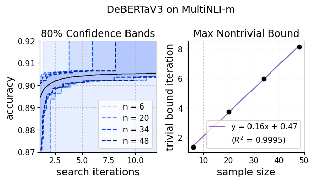
Figure 9: (left) Confidence bands for DeBERTaV3’s tuning curve on MultiNLI (matched). $n$ represents the sample size, or the number of random search iterations used in constructing the confidence bands. (right) The relationship between the sample size and the search iteration at which the upper confidence band becomes trivial. The relationship is approximately linear, with 99.95% of the variance explained.

6 Related Work

Language models’ unprecedented success creates the need for more realistic, comprehensive, and challenging evaluations (Ribeiro et al., 2020; Bowman and Dahl, 2021). As scaling reliably improves performance (Hestness et al., 2017; Rosenfeld et al., 2020; Kaplan et al., 2020; Hernandez et al., 2021), performance comparisons without consideration for cost have become inadequate (Ethayarajh and Jurafsky, 2020). There is always a bigger model with better performance. Thus, many researchers have brought attention to modern models’ considerable costs, and proposed frameworks to account for them (Strubell et al., 2019; Sharir et al., 2020; Schwartz et al., 2020; Henderson et al., 2020).

Due to hyperparameter search’s heavy compute requirements, evaluations should identify not just the best model, but the best model for a tuning budget. Many effective tuning algorithms have been proposed (Bergstra and Bengio, 2012; Snoek et al., 2012; Li et al., 2018); however, these find the best hyperparameters for a given method, rather than evaluate the method for a given budget. Beyond finding the best hyperparameters for deployment, researchers and practitioners need systematic tools to manage them during development—taking the guesswork out of evaluation. To meet this need, Dodge et al. (2019) proposed the first estimator for the expected tuning curve, or mean performance as a function of hyperparameter search iterations.

To compare models fairly, we must fix a tuning algorithm. Random search is easy to implement, a strong baseline, and the basis of several state of the art techniques (Li et al., 2018, 2020); thus, it offers a great choice for standardizing tuning curves. Insightfully, Dodge et al. (2019) leveraged the independent and identically distributed nature of random search to estimate tuning curves using V-statistics (v. Mises, 1947). V-statistics have many desirable properties; however, they can be biased, so Tang et al. (2020) introduced a complementary, unbiased estimator based on U-statistics (Hoeffding, 1948). Follow up work showed that although these estimators can disagree, neither is uniformly more correct (Dodge et al., 2021). What is more, bootstrapping these estimators fails to create valid confidence bands (Tang et al., 2020); Consequently, it is difficult to know when an estimate is reliable, versus when more data is necessary. We resolve this issue by providing the first valid confidence bands for tuning curves.

7 Conclusion

We began with a tutorial on how to tell if a method is cost-effective, well-tuned, or actually better than a baseline, using our confidence bands (§2). We then derived our simultaneous, exact, distribution-free confidence bands for tuning curves (§3). To complement this theory, we designed empirical studies (§4). These studies probed the shortcomings of existing solutions’ (§5.1), and confirmed our bands achieve the exact coverage necessary to address them (§5.2). Beyond these main results, ablations revealed how several key ideas tighten the bands (§5.3). Lastly, we investigated the effect of sample size to show the benefits of median over mean tuning curves (§5.4) and illustrate an empirical relationship that informs how many samples are needed to produce useful confidence bands (§5.5).

Hyperparameters complicate evaluation. Luckily, tuning curves let us compare methods while accounting for tuning effort. Still, point estimates leave open the question of whether or not the data is sufficient to support a given conclusion. To solve this issue, we present the first valid confidence bands for tuning curves. Our confidence bands are simultaneous, distribution-free, and achieve exact coverage in finite samples. Using these confidence bands, researchers and practitioners can compare methods reliably and reproducibly. To analyze your own experiments with confidence, try our library at https://github.com/nalourie/opda.

Limitations

While our confidence bands have many strengths, they also have limitations. Mainly, our confidence bands require that the scores are independent and identically distributed (IID), as in random search. We view random search as an ideal tool for research. In development, it can measure tuning difficulty; in production, another algorithm could find optimal hyperparameters for deployment. Still, a variant of random search, hyperband (Li et al., 2018), is competitive with state of the art. With a small modification, it can satisfy the IID assumption: just fix ahead of time the thresholds for ending training early. Finally, though random search works well in many applications, it will break down when the intrinsic dimension of the search space is high, due to the curse of dimensionality. Such models will require other techniques to assess tuning difficulty.

While this limitation is shared with prior work (Dodge et al., 2019; Tang et al., 2020; Dodge et al., 2021), our exact coverage guarantee also requires that the score distribution is continuous (the search distribution can be anything). If it is not continuous, then our KS tuning curve bands may be used, as they are conservative for discrete distributions. It is worth investigating whether the LD bands are also conservative for discrete distributions. In general, for any simultaneous confidence bands for the CDF: if the CDF bands are exact, then the median tuning curve bands will be exact as well.

Ethics Statement

We hope our confidence bands will promote more reliable and reproducible work in NLP and related sciences. Constructing tight bands requires more iterations of random search, thus more compute, than hyperparameter tuning; still, by reducing the frequency of faulty conclusions, we believe our confidence bands will ultimately save resources and produce better science in the long run.

Appendix A Proofs

If $Y$ has a continuous distribution, then both the KS and LD bands have exact coverage (Bradley, 1968; Learned-Miller and DeStefano, 2008). We will show if the CDF bands, $\widehat{F}^{l}(y)\leq F(y)\leq\widehat{F}^{u}(y)$, have exact coverage then the median tuning curve bands, $\hat{\tau}_{m}^{l}(k)\leq\tau_{m}(k)\leq\hat{\tau}_{m}^{u}(k)$, do as well:

Proposition 1.

If $\forall y,\widehat{F}^{l}(y)\leq F(y)\leq\widehat{F}^{u}(y)$ with probability $1-\alpha$, then with probability $1-\alpha$, $\forall k,\hat{\tau}_{m}^{l}(k)\leq\tau_{m}(k)\leq\hat{\tau}_{m}^{u}(k)$.

Proof.

We will show the CDF bands on $Y$ hold if and only if the tuning curve bands hold. Since the CDF bands hold with probability $1-\alpha$, the tuning curve bands will then also hold with probability $1-\alpha$.

Recall how to construct the median tuning curve confidence bands. First, take some simultaneous confidence bands for the CDF of $Y$:

$$\widehat{F}^{l}(y)\leq F(y)\leq\widehat{F}^{u}(y)$$

then, translate them into simultaneous confidence bands for the CDF of $T_{k}$ using Equation 2:

$$\widehat{F}^{l}(y)^{k} \leq F(y)^{k}\leq\widehat{F}^{u}(y)^{k}$$

$$\widehat{F}^{l}(y)^{k} \leq F_{k}(y)\leq\widehat{F}^{u}(y)^{k}$$

Thus, the CDF bands on $Y$ hold if and only if the CDF bands on $T_{k}$ hold.

Finally, we take the median of the upper band to get a lower bound, and the median of the lower band to get an upper bound:

$$\hat{\tau}_{m}^{l}(k) \coloneqq\min\left\{Y_{(i)}\mid 0.5\leq\widehat{F}^{u}\left(Y_{(i)}\right)^{k}\right\}$$

$$\hat{\tau}_{m}^{u}(k) \coloneqq\min\left\{Y_{(i)}\mid 0.5\leq\widehat{F}^{l}\left(Y_{(i)}\right)^{k}\right\}$$

Geometrically, this corresponds to drawing a horizontal line at 0.5 probability across the CDF plot, and finding where it intersects the confidence bands. Note that we only need to check the CDF bands at the order statistics since they are step functions that only change at those points.

Assume the CDF bands on $Y$ hold, then we have $\forall y,\widehat{F}^{l}(y)^{k}\leq F_{k}(y)$, so:

$$\begin{split}\Big{\{}Y_{(i)}\mid&0.5\leq\widehat{F}^{l}\left(Y_{(i)}\right)^{k}\Big{\}}\\ &\subseteq\Big{\{}Y_{(i)}\mid 0.5\leq F_{k}\left(Y_{(i)}\right)\Big{\}}\end{split}$$

Therefore:

$$\begin{split}\min\Big{\{}Y_{(i)}\mid&0.5\leq\widehat{F}^{l}\left(Y_{(i)}\right)^{k}\Big{\}}\\ &\geq\min\Big{\{}Y_{(i)}\mid 0.5\leq F_{k}\left(Y_{(i)}\right)\Big{\}}\end{split}$$

Thus:

$$\hat{\tau}_{m}^{u}(k)\geq\mathbb{M}(T_{k})$$

The case for $\hat{\tau}_{m}^{l}\leq\mathbb{M}(T_{k})$ is analogous. So, if the CDF bands hold, then the tuning curve bands hold.

For the reverse implication, assume that the CDF bands on $Y$ do not hold, then there exists some $y$ such that either $\widehat{F}^{l}(y)>F(y)$ or $F(y)>\widehat{F}^{u}(y)$. We will show the case for $\widehat{F}^{l}(y)>F(y)$. First, let $k\coloneqq\log_{F(y)}(0.5)$, so in particular $F(y)^{k}=0.5$, thus $\mathbb{M}[T_{k}]=y$. We have:

$$\widehat{F}^{l}(y)^{k}>F(y)^{k}=F(y)^{\log_{F(y)}(0.5)}=0.5$$

Consider the order statistic, $Y_{(j)}$, immediately preceding $y$. Since the score distribution is continuous, with probability 1 we have $y\not=Y_{(j)}$ and thus $Y_{(j)}<y$. Because $\widehat{F}^{l}(y)$ is a step function that only changes at the order statistics, and $Y_{(j)}$ immediately precedes $y$, we must have:

$$\widehat{F}^{l}\left(Y_{(j)}\right)^{k}=\widehat{F}^{l}(y)^{k}>0.5$$

Thus, $Y_{(j)}\in\left\{Y_{(i)}\mid 0.5\leq\widehat{F}^{l}\left(Y_{(i)}\right)^{k}\right\}$, so:

$$\hat{\tau}_{m}^{u}(k) =\min\left\{Y_{(i)}\mid 0.5\leq\widehat{F}^{l}\left(Y_{(i)}\right)^{k}\right\}$$

$$\leq Y_{(j)}$$

$$<y$$

$$=\mathbb{M}[T_{k}]$$

So, $\hat{\tau}_{m}^{u}(k)<\mathbb{M}[T_{k}]$ so the tuning curve confidence bands are violated. The other case looks similar.

Since the CDF bands for $Y$ hold if and only if the tuning curve bands hold, they hold with the same probability, $1-\alpha$. ∎

Next, we will show that the mean tuning curve confidence bands are conservative.

Proposition 2.

If $\forall y,\widehat{F}^{l}(y)\leq F(y)\leq\widehat{F}^{u}(y)$ with probability $1-\alpha$, then with probability greater than or equal to $1-\alpha$, $\forall k,\hat{\tau}_{e}^{l}(k)\leq\tau_{e}(k)\leq\hat{\tau}_{e}^{u}(k)$.

Proof.

Given two CDFs, $F(y)$ and $G(y)$, let $F(y)\preceq G(y)$ denote that the distribution for $F(y)$ is less than or equal to $G(y)$ in the usual stochastic order (i.e., first-order stochastic dominance).

Since $\forall y,\widehat{F}^{l}(y)\leq F(y)\leq\widehat{F}^{u}(y)$, we have that $\forall y,\widehat{F}^{l}(y)^{k}\leq F_{k}(y)\leq\widehat{F}^{u}(y)^{k}$. This fact is equivalent to $\widehat{F}^{u}(y)^{k}\preceq F_{k}(y)\preceq\widehat{F}^{l}(y)^{k}$. It is then a standard fact that this implies the expectation of $\widehat{F}^{l}(y)^{k}$ is greater than the expectation of $F_{k}(y)$ which is greater than the expectation of $\widehat{F}^{u}(y)^{k}$. In other words: $\hat{\tau}_{e}^{l}(k)\leq\tau_{e}(k)\leq\hat{\tau}_{e}^{u}(k)$.

Because $\forall y,\widehat{F}^{l}(y)\leq F(y)\leq\widehat{F}^{u}(y)$ implies $\forall k,\hat{\tau}_{e}^{l}(k)\leq\tau_{e}(k)\leq\hat{\tau}_{e}^{u}(k)$, the latter statement must hold with at least the probability of the former. Thus, it holds with probability at least $1-\alpha$. ∎

Unlike the median tuning curve bands, the mean tuning curve bands will be strictly conservative in general. One reason for this is that the unbounded probability mass will float to the bounds of the distribution’s support in the worst case. Another reason is that the CDF of $T_{k}$ could briefly violate its confidence bounds but still end up with a lower (or higher) mean than the upper (or lower) confidence band. Intuitively, this issue comes from the fact that unlike a quantile, which involves a single point of the CDF, the mean involves the entire shape of the CDF. Exact confidence bounds for the expected tuning curve likely require stronger assumptions.

Appendix B Experimental Setup

Expanding on §4, this appendix documents our full experimental details. For our implementation of the confidence bands and analysis, see https://github.com/nalourie/opda (tag: v0.1.0).

B.1 Comparisons to Prior Work

In our comparisons to prior work, we use the data from Tang et al. (2020) located at github.com/castorini/meanmax (commit: 0ea1241). The data contains results from hyperparameter searches for two different models: an MLP and an LSTM on the Reuters document classification dataset (Apté et al., 1994). Hyperparameter search was run for 145 iterations on the MLP and 152 iterations on the LSTM, using F1 score as the validation metric.

For the MLP, the search distribution was uniform over {16, 32, 64} for the batch size, a learning rate of 0.001, discrete uniform over 0-$10^{7}$ for the random seed, uniform over $[0.05,0.7]$ for the dropout rate, 1 hidden layer, and discrete uniform over 256-768 for the hidden dimension.

The LSTM had a nonstandard hyperparameter. For it, "static" initialized word embeddings with frozen word2vec vectors (Mikolov et al., 2013), "nonstatic" initialized word embeddings with trainable word2vec vectors, and "rand" initialized word embeddings randomly. For the LSTM, the search distribution was static, nonstatic, or rand with a 40%, 50%, and 10% chance, uniform over {16, 32, 64} for batch size, a truncated exponential over $[0.001,0.099]$ for learning rate, a discrete uniform over 0-$10^{7}$ for the random seed, 1 or 2 layers with a 75% and 25% chance, discrete uniform over 384-768 for hidden dimension, a uniform over $[0,0.3]$ for weight dropout rate, a uniform over $[0,0.3]$ for embedding dropout rate, and a uniform over $[0.985,0.995]$ for the coefficient to use in exponentially averaging the parameters.

For our kernel density estimates (KDEs), we used a Gaussian kernel with reflection about the support’s boundary (0 and 1 for F1 score) as a boundary correction (Jones, 1993). We selected the bandwidth from the grid: 1.00e-1, 5.00e-2, 2.50e-2, 1.25e-2, and 6.25e-3, by visually inspecting the PDF and CDF plots for the resulting KDE. Ultimately, we chose 5.00e-2 and 1.25e-2 for the LSTM and MLP KDE bandwidths, respectively.

In our simulation for computing the bootstrap confidence bands’ coverage, we ran 4,096 rounds, in each round testing whether or not the bootstrap confidence bands covered the true tuning curve at each point. To construct the bootstrap confidence bands, we sampled 50 points from the simulated score distribution and then resampled this initial sample 4,096 times to determine the bootstrap distribution’s quantiles for the different estimators at each point of the tuning curve.

B.2 Analysis in a Realistic NLP Scenario

For our analysis of a realistic NLP scenario, we train DeBERTa (He et al., 2021b) and DeBERTaV3 (He et al., 2021a) using the original DeBERTa codebase: github.com/microsoft/DeBERTa (commit: c558ad9). Specifically, we fine-tuned DeBERTa-base and DeBERTaV3-base on MultiNLI (Williams et al., 2018) and evaluated using accuracy. For both models, we ran 1,024 rounds of random search and used the same search distribution for each.

The search distribution was discrete uniform over 16-64 for batch size, discrete uniform over 1-4 for number of epochs, uniform over $[0,0.6]$ for warmup proportion of the first epoch, log uniform over $[10^{-6},10^{-3}]$ for learning rate, and uniform over $[0,0.3]$ for dropout rate. For ease of comparison, we used the same sample of 1,024 hyperparameters for both models. For other implementation details, we used the fp16 floating point format, a maximum sequence length of 256, an evaluation batch size of 256, and we logged progress every 1000 steps. All other hyperparameters were identical to DeBERTa and DeBERTaV3’s defaults for MultiNLI.

Each training run for DeBERTa or DeBERTaV3 on a given set of hyperparameters was run via SLURM with a single RTX 8000 NVIDIA GPU (48 GB), 2 CPU cores from an Intel Xeon Platinum 8268 Processor (2.90 GHz), and 32 GB of CPU memory. For software, the code was run on Ubuntu 18.04.5 LTS with CUDA V10.1.243, Conda 32.1.0, Python 3.7.16, and PyTorch 1.7.0.

Hyperparameter tuning jobs were run in parallel. For DeBERTa-base, the jobs took an average of 4h 57m 57s with a standard deviation of 2h 19m 0s, a minimum of 1h 43m 28s, and a maximum of 11h 9m 8s. For DeBERTaV3-base, the jobs took an average of 4h 8m 30s with a standard deviation of 1h 56m 50s, a minimum of 1h 24m 57s, and a maximum of 9h 29m 38s.

For the tutorial on evaluating DeBERTaV3 (§2), we subsampled 48 hyperparameter evaluations without replacement from the total 1,024 for both DeBERTa and DeBERTaV3 in order to construct tuning curves with confidence bands.

For our kernel density estimates (KDEs), we used a Gaussian kernel. Due to the large sample sizes (1,024 samples for both DeBERTa and DeBERTaV3), the amount of probability mass outside the support’s bounds (0 and 1 for accuracy) was smaller than the numerical precision; therefore, we did not need to apply a boundary correction to the KDE. We selected the bandwidth from the grid: 1.0e-1, 7.5e-2, 5e-2, and 2.5e-2, by visually inspecting the PDF and CDF plots for the resulting KDE. Ultimately, we chose 5e-2 as the bandwidth for both DeBERTa and DeBERTaV3’s simulations.

To estimate the median tuning curve confidence bands’ empirical coverage, we ran 1,024 rounds of simulation. In each round, we sampled 48 scores from the kernel density estimate, constructed the median tuning curve confidence bands, and then measured how often the entire median tuning curve was covered simultaneously. Because the CDF and median tuning curve are increasing and their confidence bands are step functions, it’s only necessary to check for violations around the discontinuities.

Appendix C Additional Algorithms

In §3.3, Equation 10 defines the test statistic, $L_{n}$:

$$L_{n}\coloneqq\max_{i=1\ldots n}B_{i}\left(F\left(Y_{(i)}\right)\right)$$

Where $B_{i}\left(p\right)$ is coverage under $\text{Beta}(i,n{+}1{-}i)$ of the smallest (equal-tailed or highest density) interval containing $p$. To compute $L_{n}$ or construct confidence bands for a given value of $L_{n}$, we then need the ability to compute (equal-tailed or highest density) intervals for the beta distribution, and to compute the coverage of the smallest such interval containing a point $p$. We describe algorithms for these tasks here. For full implementation details, see the code at https://github.com/nalourie/opda (tag: v0.1.0).

Recall that when $a>1$ or $b>1$, $\text{Beta}(a,b)$ is unimodal, making the highest density interval well-defined. The mode is then $p^{*}=\frac{a-1}{a+b-2}$. We are only interested in the distributions $\text{Beta}(i,n{+}1{-}i)$, thus whenever we have two or more samples the distributions will all be unimodal. Many statistical packages make available the beta’s density, $g(p)$, CDF, $G(p)$, and inverse CDF or quantile function, $G^{-1}(u)$, so we assume access to these functions.

C.1 Intervals

Given a $\text{Beta}(a,b)$ distribution, we would like to compute intervals for it that contain $1-\alpha$ of the probability mass.

The equal-tailed interval may be computed from the inverse CDF directly:

$$\left[G^{-1}\left(\frac{\alpha}{2}\right),G^{-1}\left(1-\frac{\alpha}{2}\right)\right]$$

The highest density interval is more challenging. Given a lower end point, $p_{l}$, we can construct the interval with coverage $1-\alpha$ by setting the upper end point, $p_{u}$, to:

$$p_{u}=G^{-1}\left(G\left(p_{l}\right)+1-\alpha\right)$$

This is the highest density interval with coverage $1-\alpha$ precisely when the density is equal at the end points:

$$g(p_{l})=g(p_{u})$$

Thus, we can use any root finding algorithm to identify the value of $p_{l}$ for which the end points have equal density. In other words, we solve the following equation for $p_{l}$:

$$g(p_{l})-g\left(G^{-1}\left(G\left(p_{l}\right)+1-\alpha\right)\right)=0$$

Our implementation uses the bisection method (i.e., binary search) due to its simplicity and robustness. Letting $p^{*}=\frac{a-1}{a+b-2}$ (the mode), we initialize the lower bound for $p_{l}$ to:

$$G^{-1}\left(\max\left\{G\left(p^{*}\right)-(1-\alpha),0\right\}\right)$$

and we initialize the upper bound for $p_{l}$ to:

$$\min\left\{p^{*},G^{-1}\left(\alpha\right)\right\}$$

We then use binary search to shrink the interval to within some tolerance.

C.2 Coverage

To compute the $L_{n}$ statistic, we need to compute the coverage under $\text{Beta}(a,b)$ of the smallest equal-tailed or highest density interval containing $p$.

Given $p$, the equal-tailed interval’s coverage is:

$$2\left|\frac{1}{2}-G(p)\right|$$

The highest density interval requires finding a root. The smallest highest density interval containing $p$ either has $p$ as the lower or the upper endpoint. We can identify which it is by comparing $p$ with the mode, $p^{*}$. Consider when $p=p_{l}$, or $p$ is the lower endpoint. The upper end, $p_{u}$, must have the same density as the lower, so it satisfies the equation:

$$g\left(p\right)-g\left(p_{u}\right)=0$$

We could solve this equation using any root finding algorithm. Our implementation uses the bisection method (binary search), initializing the bounds to $0$ and $p^{*}$ when seeking the lower end, and $p^{*}$ and $1$ when seeking the upper end.

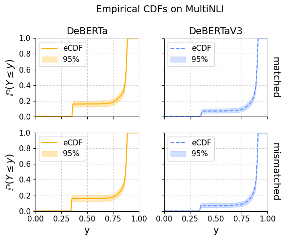
Figure 10: Highest density LD bands for the samples of 1,024 search iterations described in §4 and §B.2.

We experimented with a number of root finding algorithms (the bisection method, secant method, regula falsi, Newton’s method, hybridizations); however, a good implementation of the bisection method proved fastest and most practical due to its reliability. Because we need to find roots for many different beta distributions when constructing the confidence bands, the faster convergence of Newton’s method failed to make up for the cost of recovering from failures to converge when performing the algorithm in a vectorized way, though perhaps better implementations could improve upon this.

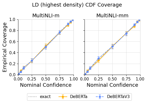
Figure 11: Nominal vs. empircal coverage of the LD CDF bands for the score distribution. Error bars show 99% Clopper-Pearson confidence intervals. The results lie on the $y=x$ line, indicating exact coverage.

Appendix D Exact Coverage Results

In §5.2, we simulate a practical hyperparameter tuning scenario by first running random search on DeBERTa and DeBERTaV3 1,024 times each, then using the resulting data for kernel density estimates of the true distributions. To realistically simulate these scenarios, we need a sample size that’s large enough to guarantee a close approximation to the underlying distributions. Our samples do in fact achieve such approximations, as shown by the simultaneous 95% confidence bands for the CDFs presented in Figure 10. Since the confidence bands are so narrow, we can conclude the samples’ eCDFs adhere tightly to the true CDFs.

In addition to the LD tuning curve confidence bands, we empirically validated the LD CDF bands’ coverage. Figure 11 confirms the LD CDF bands, and in particular our implementation via inverting the hypothesis test, achieve exact coverage.

Appendix E Extended Results and Ablation Studies

Expanding on §5.3, we provide extended ablation results. In general, the conclusions mirror those of §5.3. Figure 12 and Figure 14 respectively introduce new results by comparing the CDF bands (as opposed to tuning curves) from the DKW, KS, and LD methods and the equal-tailed and highest density intervals. Figure 13 and Figure 15 expand on the existing results by respectively comparing the DKW, KS, and LD methods and the equal-tailed and highest density intervals for more sample sizes. For even more results, see the jupyter notebooks located at https://github.com/nalourie/opda (tag: v0.1.0).

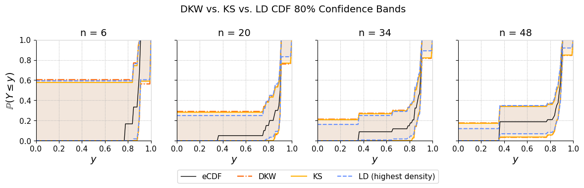
Figure 12: DKW, KS, and LD confidence bands for DeBERTaV3’s score distribution on MultiNLI (matched).

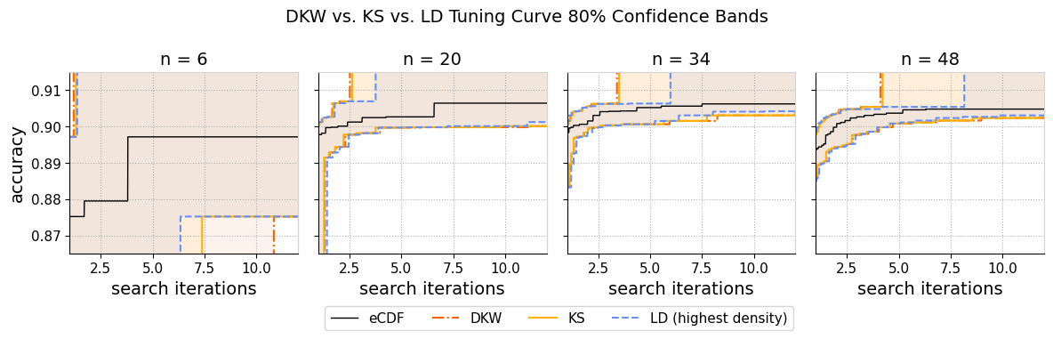
Figure 13: DKW, KS, and LD confidence bands for DeBERTaV3’s tuning curve on MultiNLI (matched).

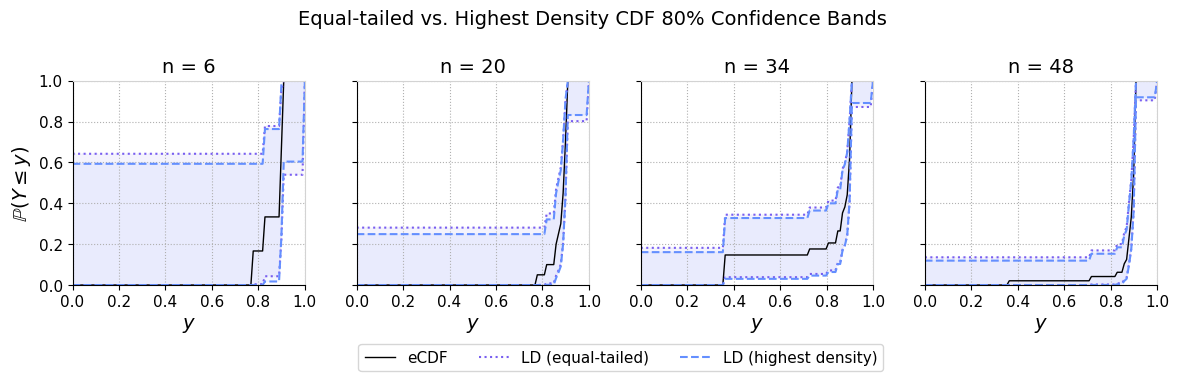
Figure 14: Equal-tailed and highest density LD bands for DeBERTaV3’s score distribution on MultiNLI (matched).

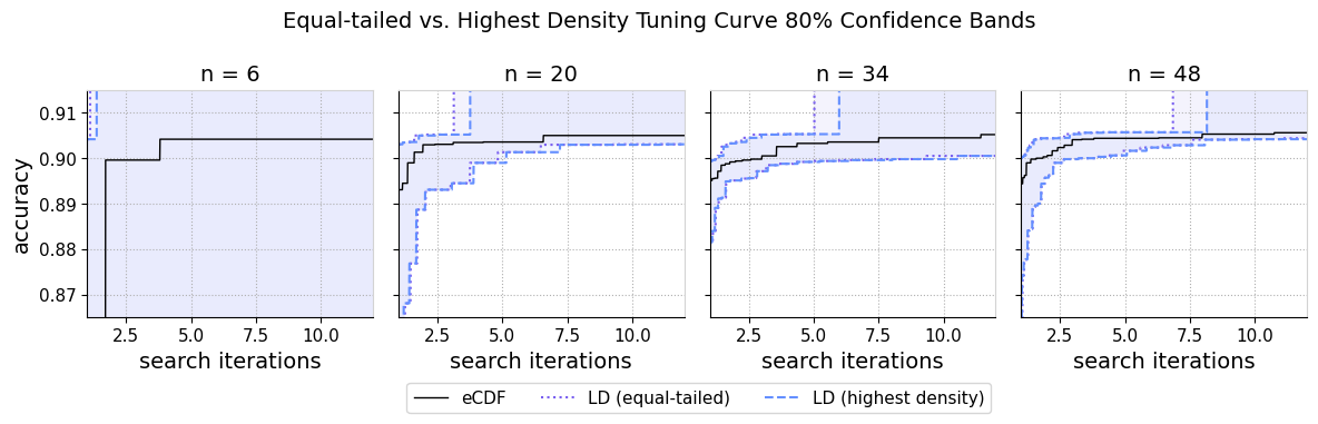
Figure 15: Equal-tailed and highest density LD bands for DeBERTaV3’s tuning curve on MultiNLI (matched).

References

- Apté et al. (1994) Chidanand Apté, Fred Damerau, and Sholom M. Weiss. 1994. Automated learning of decision rules for text categorization. ACM Trans. Inf. Syst., 12(3):233–251.
- Bergstra and Bengio (2012) James Bergstra and Yoshua Bengio. 2012. Random search for hyper-parameter optimization. Journal of Machine Learning Research, 13(10):281–305.
- Bowman and Dahl (2021) Samuel R. Bowman and George Dahl. 2021. What will it take to fix benchmarking in natural language understanding? In Proceedings of the 2021 Conference of the North American Chapter of the Association for Computational Linguistics: Human Language Technologies, pages 4843–4855, Online. Association for Computational Linguistics.
- Bradley (1968) J.V. Bradley. 1968. Distribution-free Statistical Tests. Prentice-Hall.
- Dodge et al. (2019) Jesse Dodge, Suchin Gururangan, Dallas Card, Roy Schwartz, and Noah A. Smith. 2019. Show your work: Improved reporting of experimental results. In Proceedings of the 2019 Conference on Empirical Methods in Natural Language Processing and the 9th International Joint Conference on Natural Language Processing (EMNLP-IJCNLP), pages 2185–2194, Hong Kong, China. Association for Computational Linguistics.
- Dodge et al. (2021) Jesse Dodge, Suchin Gururangan, Dallas Card, Roy Schwartz, and Noah A. Smith. 2021. Expected validation performance and estimation of a random variable’s maximum. In Findings of the Association for Computational Linguistics: EMNLP 2021, pages 4066–4073, Punta Cana, Dominican Republic. Association for Computational Linguistics.
- Dvoretzky et al. (1956) A. Dvoretzky, J. Kiefer, and J. Wolfowitz. 1956. Asymptotic Minimax Character of the Sample Distribution Function and of the Classical Multinomial Estimator. The Annals of Mathematical Statistics, 27(3):642 – 669.
- Efron and Tibshirani (1994) B. Efron and R.J. Tibshirani. 1994. An Introduction to the Bootstrap. Chapman and Hall/CRC.
- Ethayarajh and Jurafsky (2020) Kawin Ethayarajh and Dan Jurafsky. 2020. Utility is in the eye of the user: A critique of NLP leaderboards. In Proceedings of the 2020 Conference on Empirical Methods in Natural Language Processing (EMNLP), pages 4846–4853, Online. Association for Computational Linguistics.
- He et al. (2021a) Pengcheng He, Jianfeng Gao, and Weizhu Chen. 2021a. Debertav3: Improving deberta using electra-style pre-training with gradient-disentangled embedding sharing.
- He et al. (2021b) Pengcheng He, Xiaodong Liu, Jianfeng Gao, and Weizhu Chen. 2021b. Deberta: Decoding-enhanced bert with disentangled attention. In International Conference on Learning Representations.
- Henderson et al. (2020) Peter Henderson, Jieru Hu, Joshua Romoff, Emma Brunskill, Dan Jurafsky, and Joelle Pineau. 2020. Towards the systematic reporting of the energy and carbon footprints of machine learning. Journal of Machine Learning Research, 21(248):1–43.
- Hernandez et al. (2021) Danny Hernandez, Jared Kaplan, Tom Henighan, and Sam McCandlish. 2021. Scaling laws for transfer.
- Hestness et al. (2017) Joel Hestness, Sharan Narang, Newsha Ardalani, Gregory Diamos, Heewoo Jun, Hassan Kianinejad, Md. Mostofa Ali Patwary, Yang Yang, and Yanqi Zhou. 2017. Deep learning scaling is predictable, empirically.
- Hoeffding (1948) Wassily Hoeffding. 1948. A Class of Statistics with Asymptotically Normal Distribution. The Annals of Mathematical Statistics, 19(3):293 – 325.
- Hoffmann et al. (2022) Jordan Hoffmann, Sebastian Borgeaud, Arthur Mensch, Elena Buchatskaya, Trevor Cai, Eliza Rutherford, Diego de Las Casas, Lisa Anne Hendricks, Johannes Welbl, Aidan Clark, Thomas Hennigan, Eric Noland, Katherine Millican, George van den Driessche, Bogdan Damoc, Aurelia Guy, Simon Osindero, Karén Simonyan, Erich Elsen, Oriol Vinyals, Jack Rae, and Laurent Sifre. 2022. An empirical analysis of compute-optimal large language model training. In Advances in Neural Information Processing Systems, volume 35, pages 30016–30030. Curran Associates, Inc.
- Jones (1993) M.C. Jones. 1993. Simple boundary correction for kernel estimation. Statistics and Computing, 3:135–146.
- Kaplan et al. (2020) Jared Kaplan, Sam McCandlish, Tom Henighan, Tom B. Brown, Benjamin Chess, Rewon Child, Scott Gray, Alec Radford, Jeffrey Wu, and Dario Amodei. 2020. Scaling laws for neural language models.
- Learned-Miller and DeStefano (2008) E. Learned-Miller and J. DeStefano. 2008. A probabilistic upper bound on differential entropy. IEEE Trans. Inf. Theor., 54(11):5223–5230.
- Li et al. (2018) Liam Li, Kevin Jamieson, Giulia DeSalvo, Afshin Rostamizadeh, and Ameet Talwalkar. 2018. Hyperband: A novel bandit-based approach to hyperparameter optimization. Journal of Machine Learning Research, 18-185:1–52.
- Li et al. (2020) Liam Li, Kevin Jamieson, Afshin Rostamizadeh, Ekaterina Gonina, Jonathan Ben-tzur, Moritz Hardt, Benjamin Recht, and Ameet Talwalkar. 2020. A system for massively parallel hyperparameter tuning. In Proceedings of Machine Learning and Systems, volume 2, pages 230–246.
- Massart (1990) P. Massart. 1990. The Tight Constant in the Dvoretzky-Kiefer-Wolfowitz Inequality. The Annals of Probability, 18(3):1269 – 1283.
- Mikolov et al. (2013) Tomas Mikolov, Ilya Sutskever, Kai Chen, Greg Corrado, and Jeffrey Dean. 2013. Distributed representations of words and phrases and their compositionality. In Proceedings of the 26th International Conference on Neural Information Processing Systems - Volume 2, NIPS’13, page 3111–3119, Red Hook, NY, USA. Curran Associates Inc.
- Minka (2002) Thomas P. Minka. 2002. Judging significance from error bars. Technical report, MIT.
- Ribeiro et al. (2020) Marco Tulio Ribeiro, Tongshuang Wu, Carlos Guestrin, and Sameer Singh. 2020. Beyond accuracy: Behavioral testing of NLP models with CheckList. In Proceedings of the 58th Annual Meeting of the Association for Computational Linguistics, pages 4902–4912, Online. Association for Computational Linguistics.
- Rosenfeld et al. (2020) Jonathan S. Rosenfeld, Amir Rosenfeld, Yonatan Belinkov, and Nir Shavit. 2020. A constructive prediction of the generalization error across scales. In International Conference on Learning Representations.
- Schwartz et al. (2020) Roy Schwartz, Jesse Dodge, Noah A. Smith, and Oren Etzioni. 2020. Green AI. Communications of the ACM (CACM), 63(12):54–63.
- Sharir et al. (2020) Or Sharir, Barak Peleg, and Yoav Shoham. 2020. The cost of training nlp models: A concise overview.
- Snoek et al. (2012) Jasper Snoek, Hugo Larochelle, and Ryan P Adams. 2012. Practical bayesian optimization of machine learning algorithms. In Advances in Neural Information Processing Systems, volume 25. Curran Associates, Inc.
- Strubell et al. (2019) Emma Strubell, Ananya Ganesh, and Andrew McCallum. 2019. Energy and policy considerations for deep learning in NLP. In Proceedings of the 57th Annual Meeting of the Association for Computational Linguistics, pages 3645–3650, Florence, Italy. Association for Computational Linguistics.
- Tang et al. (2020) Raphael Tang, Jaejun Lee, Ji Xin, Xinyu Liu, Yaoliang Yu, and Jimmy Lin. 2020. Showing your work doesn’t always work. In Proceedings of the 58th Annual Meeting of the Association for Computational Linguistics, pages 2766–2772, Online. Association for Computational Linguistics.
- v. Mises (1947) R. v. Mises. 1947. On the Asymptotic Distribution of Differentiable Statistical Functions. The Annals of Mathematical Statistics, 18(3):309 – 348.
- Vaart (1998) A. W. van der Vaart. 1998. Asymptotic Statistics. Cambridge Series in Statistical and Probabilistic Mathematics. Cambridge University Press.
- Williams et al. (2018) Adina Williams, Nikita Nangia, and Samuel Bowman. 2018. A broad-coverage challenge corpus for sentence understanding through inference. In Proceedings of the 2018 Conference of the North American Chapter of the Association for Computational Linguistics: Human Language Technologies, Volume 1 (Long Papers), pages 1112–1122, New Orleans, Louisiana. Association for Computational Linguistics.