First Sagittarius A^∗ Event Horizon Telescope Results III: Imaging of the Galactic Center Supermassive Black Hole

Abstract

We present the first event-horizon-scale images and spatiotemporal analysis of Sgr A^∗ taken with the Event Horizon Telescope in 2017 April at a wavelength of 1.3 mm. Imaging of Sgr A^∗ has been conducted through surveys over a wide range of imaging assumptions using the classical CLEAN algorithm, regularized maximum likelihood methods, and a Bayesian posterior sampling method. Different prescriptions have been used to account for scattering effects by the interstellar medium towards the Galactic Center. Mitigation of the rapid intra-day variability that characterizes Sgr A^∗ has been carried out through the addition of a “variability noise budget" in the observed visibilities, facilitating the reconstruction of static full-track images. Our static reconstructions of Sgr A^∗ can be clustered into four representative morphologies that correspond to ring images with three different azimuthal brightness distributions, and a small cluster that contains diverse non-ring morphologies. Based on our extensive analysis of the effects of sparse $(u,v)$-coverage, source variability and interstellar scattering, as well as studies of simulated visibility data, we conclude that the Event Horizon Telescope Sgr A^∗ data show compelling evidence for an image that is dominated by a bright ring of emission with a ring diameter of $\sim$50 $\mu$as, consistent with the expected “shadow" of a $4\times 10^{6}M_{\odot}$ black hole in the Galactic Center located at a distance of 8 kpc.

1 Introduction

At the center of our galaxy is the nearest candidate supermassive black hole (SMBH), Sagittarius A* (Sgr A^∗). We present here the first horizon-scale images of it. Compared with M87^∗, Sgr A^∗ is more challenging to image mainly due to its rapid variability and the distortions of the intervening scattering medium. We develop methods to characterize and mitigate these two factors in order to reconstruct images that take us a step closer to establishing that Sgr A^∗ is a black hole. This paper is the third in the Event Horizon Telescope (EHT)’s series of six Sgr A^∗ articles (Event Horizon Telescope Collaboration et al., 2022a, b, c, d, e, f, hereafter Papers I, II, III, IV, V, and VI).

Since the first discovery of Sgr A^∗ as a compact radio source with interferometric observations at centimeter (cm) wavelengths (Balick & Brown, 1974), there have been many studies of this closest SMBH to Earth. Of particular importance is the study of stellar dynamics showing that the position of Sgr A^∗ in the Galactic Center coincides with the center of gravity of a dense cluster of young and old stars (Eckart & Genzel, 1997; Ghez et al., 1998; Menten et al., 1997; Reid & Brunthaler, 2004; Reid, 2009). Moreover, the gravitational potential is dominated by a compact object of mass of $4\times 10^{6}M_{\odot}$ contained within 120 AU of Sgr A^∗, at a distance of 8 kpc from Earth (Ghez et al., 2008; Gillessen et al., 2009, 2017; Gravity Collaboration et al., 2018b, 2019; Do et al., 2019). Based on these facts, together with the continuous variability on characteristic time scales from minutes to hours, especially at near-infrared (NIR) wavelengths on angular scales of typically 150 micro-arcseconds ($\mu$as) (Gravity Collaboration et al., 2018a, 2020), the likely scenario of Sgr A^∗ is that this compact object is a SMBH. The combination of mass and proximity make Sgr A^∗ the black hole subtending the largest angle on the sky with a Schwarzschild radius of 0.08 AU$\,\sim 10\,\mu$as and an expected “shadow” angular size of $\sim 50\,\mu$as. Sgr A^∗ was thus identified early on as a primary target for imaging a black hole “shadow” (Falcke et al., 2000) predicted by Einstein’s theory of general relativity (Hilbert, 1917; von Laue, 1921; Bardeen, 1973; Luminet, 1979). Similar calculations put the shadow angular size of M87^∗ at $\sim 40\,\mu$as ($6.5\times 10^{9}M_{\odot}$, 16.4 Mpc from Earth) confirmed by the EHT through imaging and analysis (Event Horizon Telescope Collaboration et al., 2019a, b, c, d, e, f, hereafter M87^∗ Papers I-VI).

In very-long-baseline interferometry (VLBI) observations at cm wavelengths, the structure of Sgr A^∗ is unresolved and dominated by scatter broadening caused by the ionized interstellar medium (ISM; see, e.g., Rickett 1990; Narayan 1992). As a result, the measured sizes are proportional to $\lambda^{2}$, where $\lambda$ is the observing wavelength (Davies et al., 1976), with an asymmetric Gaussian shape elongated toward the east-west direction (i.e., stronger angular broadening; Lo et al. 1985, 1998; Alberdi et al. 1993; Krichbaum et al. 1993; Frail et al. 1994; Bower & Backer 1998). For several decades, many VLBI observations have attempted to reach smaller angular (and spatial) scales. These studies found that the observed size at millimeter (mm) wavelengths deviates from the $\lambda^{2}$-relation, indicating a larger intrinsic size than expected from scatter broadening of an intrinsically unresolved source (e.g., Krichbaum et al., 1998; Lo et al., 1998; Doeleman et al., 2008; Falcke et al., 2009).

After constraining the scattering effects (see Section 3.1), the intrinsic structure of Sgr A^∗ at long radio wavelengths can be modelled with a single nearly isotropic Gaussian source (Bower et al., 2004; Shen et al., 2005; Lu et al., 2011a; Bower et al., 2014; Johnson et al., 2018; Issaoun et al., 2021; Cho et al., 2022). Its size and orientation on the sky have remained fairly constant over days to years timescales (e.g., Alberdi et al., 1993; Marcaide et al., 1999; Lu et al., 2011b), but a marginal variation has also been suggested (Bower et al. 2004; Akiyama et al. 2013). At observing wavelengths $>1\,$mm, some evidence for structure beyond a single Gaussian model has also been reported. While this is likely attributed to refractive scattering sub-structure (i.e., not intrinsic) at cm-wavelengths (e.g., Gwinn et al., 2014), its cause is still unclear at mm-wavelengths. For instance, at 7 mm, Rauch et al. (2016) reported a short-lived secondary component that could possibly be related to a preceding NIR flare. However, the detection of non-zero closure phases was only marginal, and does not exclude a realization of thermal or other systematic errors. At 3.5 mm, several studies have found slight non-zero closure phases (Ortiz-León et al., 2016; Brinkerink et al., 2016) and asymmetric non-Gaussian structure along the minor axis (Issaoun et al., 2019, 2021), but its physical origin remained non-conclusive: it could be due either to scattering or an intrinsic asymmetry of Sgr A^∗.

Multi-wavelength observations of Sgr A^∗ show an inverted spectral energy distribution rising with frequency in the radio due to synchrotron emission, with spectral break at THz frequencies (submillimeter wavelengths), where the accretion flow becomes optically thin (Falcke et al., 1998; Bower et al., 2015, 2019). Its bolometric luminosity was measured to be $\sim 5\times 10^{35}\,{\rm erg\,s}^{-1}$, or $10^{-9}L_{\rm Edd}$ (Genzel et al., 2010; Bower et al., 2019). A more detailed description of the spectral properties of Sgr A^∗ is presented in Paper II. At an observing frequency of 230 GHz (1.3 mm wavelength), the accretion flow is expected to be sufficiently optically thin to detect the black hole shadow in Sgr A^∗ with an Earth-sized interferometric array, such as the Event Horizon Telescope (EHT) (Falcke et al. 2000; Doeleman et al. 2009; Broderick et al. 2016; M87^∗ Paper II).

Sgr A^∗ additionally exhibits variability across the entire electromagnetic spectrum (Genzel et al., 2003; Ghez et al., 2004; Neilsen et al., 2013, 2015; Bower et al., 2015; Boyce et al., 2019), with frequent flaring in the radio, infrared and X-ray regimes. Variability and motion can be observed within a single observing night, with variability timescales of the order of seconds to hours, characteristic dynamic timescales for a $4\times 10^{6}M_{\odot}$ black hole (Baganoff et al., 2003; Marrone et al., 2006; Meyer et al., 2008; Hora et al., 2014; Dexter et al., 2014; Witzel et al., 2018; Bower et al., 2018, 2019). In the radio and submillimeter, Sgr A^∗ is constantly varying, with a variability level of $<10\%$ during quiescence (Macquart & Bower 2006; Paper II; Wielgus et al., 2022). A detailed description of the multi-wavelength properties of Sgr A^∗ is presented in Paper II.

At 1.3 mm, Sgr A^∗ was detected for the first time with VLBI on a single baseline with the IRAM 30-m telescope and the Plateau de Bure Interferometer in 1995 (Krichbaum et al., 1998). In 2007, the first successful observations with the early EHT array, consisted of the Arizona Radio Observatory Sub-Millimeter Telescope (SMT) in Arizona, the James Clerk Maxwell Telescope (JCMT) in Hawaiʻi and the Combined Array for Research in Millimeter-wave Astronomy (CARMA) in California, offered the first line of evidence that the source size at 1.3 mm is comparable to the expected size of the shadow of a SMBH with the mass and position of Sgr A^∗ (Doeleman et al., 2008; Fish et al., 2011). In 2013, 1.3 mm observations were carried out with an early subset of the present EHT array: five stations at four geographical sites (Arizona, California, Hawaiʻi, and Chile). An early processing of the US-only data resulted in a first measurement of relatively high linear polarization on the $50-100\,\mu$as scale by Johnson et al. (2015), and the detection of non-zero closure phases by Fish et al. (2016), indicative of asymmetric source structure on the Arizona–California–Hawaiʻi triangle. A final processing of the data with the addition of Atacama Pathfinder Experiment telescope (APEX) in Chile, by Lu et al. (2018), which provides a resolution of $\sim 30\,\mu$as (3 Schwarzschild Radii for the estimated black hole mass) in the north-south direction, revealed the presence of compact structure residing within the scale of $50\,\mu$as and confirmed the previously reported asymmetry (non-zero closure phase) by Fish et al. (2016). A subsequent expansion effort of the EHT to increase array sensitivity and imaging ability culminated in the April 2017 EHT observing campaign (M87^∗ Paper II).

The 2017 EHT observing campaign was scheduled over a 12-day time window in April 2017, to minimize weather impact. The two primary targets, M87^∗ (at the center of the giant elliptical galaxy M87) and Sgr A^∗, were observed for four and five nights, respectively. With a similar mass-to-distance ratio, the two targets are expected to exhibit similar angular sizes on the sky. Because M87^∗ is about three orders of magnitude more massive compared to Sgr A^∗, its dynamical timescale is much longer, allowing for the straightforward use of standard aperture synthesis VLBI techniques over each observing night. The effects of scattering toward the M87 galaxy are also minimal. These factors render M87^∗ the optimal first imaging target for the EHT. Based on the observations of M87^∗ the EHT Collaboration presented first direct images of a SMBH, showing a bright ring-like structure surrounding a central dark circular area (; ; ; ; ; ). Under the stellar dynamics mass measurement prior (Gebhardt et al., 2011) and with a scaling based on numerical simulations of the accretion flow (M87^∗ Paper V), these images confirm the predictions of general relativity about the diameter of a black hole shadow (M87^∗ Paper VI). Following these results, the analysis of the linear polarization observations of M87^∗ produced the first polarized images of the M87^∗ black hole and inferred a magnetic field strength and geometry in the immediate vicinity of the SMBH (Event Horizon Telescope Collaboration et al., 2021a, b, hereafter M87^∗ Papers VII and VIII). The technique and workflow developments for the analysis of M87^∗ data serve as the basis for Sgr A^∗ analysis, although new significant developments were introduced to address the challenges of interstellar scattering and short-timescale variability.

In this paper, we present the first imaging results of Sgr A^∗ with the EHT for the 2017 April 6 and 7 observations. In Section 2, we describe the EHT observations of Sgr A^∗ in 2017 and their properties. In Section 3, we estimate additional properties of two major effects anticipated for Sgr A^∗, interstellar scattering and intrinsic intra-day brightness variations, from non-imaging analysis to aid the imaging process. In Section 4, we provide a brief review of the employed imaging techniques. In Section 5, we describe the process for synthetic data generation for the imaging parameter surveys outlined in Section 6. These surveys provide a set of imaging parameters that are used to produce Sgr A^∗ images. In Section 7, we describe the resulting Sgr A^∗ images for four different imaging pipelines and assess their properties and uncertainties. In Section 8, we extract source parameters from Sgr A^∗ images via ring parameter fitting. In Section 9, we utilize dynamical imaging and geometric modeling techniques to explore and characterize potential azimuthal time variations in the data. We summarize our results in Section 10.

2 Observations and Data Processing

In this section we describe the EHT observations of Sgr A^∗ performed in 2017 April (Section 2.1), the data reduction (Section 2.2), and overall data properties (Section 2.3). A description of interferometric measurements and associated data products is provided in M87^∗ Paper IV for reference.

2.1 EHT Observations

The EHT observed Sgr A^∗ with eight stations at six geographic sites on 2017 April 5, 6, 7, 10, and 11. The participating radio observatories are the phased Atacama Large Millimeter/submillimeter Array (ALMA) and APEX in the Atacama Desert in Chile, the JCMT and the phased Submillimeter Array (SMA) on Maunakea in Hawaiʻi, the SMT on Mt. Graham in Arizona, the IRAM 30-m (PV) telescope on Pico Veleta in Spain, the Large Millimeter Telescope Alfonso Serrano (LMT) on the Sierra Negra in Mexico, and the South Pole Telescope (SPT) in Antarctica. The observations of Sgr A^∗ were interleaved with two AGN calibrator sources, the quasars NRAO 530 and J1924-2914. Scientific analysis of the observations of calibrators will be presented in future publications (Jorstad et al. in prep., Issaoun et al. in prep.). The geocentric coordinates for each of the telescopes are presented in Table 2 of M87^∗ Paper II.

The 2017 VLBI data were recorded in two polarizations and two frequency bands at a total data rate of 32 Gbps (for 2 bit sampling). All sites recorded two 2 GHz wide frequency windows centered at 227.1 and 229.1 GHz, low and high band respectively. An extensive description of the EHT array setup, equipment, and station upgrades leading up to the 2017 observations is provided in M87^∗ Paper II. All sites except ALMA and JCMT recorded dual circular polarization (RCP and LCP). ALMA recorded dual linear polarization, subsequently converted to a circular basis via the CASA-based software package PolConvert (Martí-Vidal et al., 2016; Matthews et al., 2018; Goddi et al., 2019), and JCMT recorded a single circular polarization (the recorded polarization component varied from day to day). Since JCMT recorded a single circular polarization, baselines to JCMT use the available parallel-hand component ($RR$ or $LL$) visibilities to approximate Stokes $\mathcal{I}$ (“pseudo $\mathcal{I}$”, $\mathcal{I}\equiv RR\equiv LL$). This is consistent with the Stokes $\mathcal{V}\equiv 0$ assumption taken for the data calibration, justified by the expected $|\mathcal{I}|\gg|\mathcal{V}|$ relation (Muñoz et al., 2012; Goddi et al., 2021). A small but detectable amount of intrinsic circular source polarization is present in our observations, which we account for in the systematic error analysis (Paper II).

2.2 Data Reduction

Following the correlation of the data recorded at different sites, instrumental bandpass effects and phase turbulence introduced by the Earth’s atmosphere were corrected using established fringe fitting algorithms (M87^∗ Paper III). We use two independent software packages, the CASA-based (McMullin et al., 2007) rPICARD pipeline (Janssen et al., 2019) and the HOPS-based (Whitney et al., 2004) EHT-HOPS pipeline (Blackburn et al., 2019). The mitigation of the atmospheric phase variation allows for coherent averaging of the data in order to build up signal-to-noise ratio (S/N) without substantial losses from decoherence. Instrumental RCP/LCP phase and delay offsets were corrected by referencing fringe solutions to ALMA, calibrated with PolConvert (Martí-Vidal et al., 2016). The assumption of Stokes $\mathcal{V}=0$ on VLBI baselines is taken for the RCP/LCP gain calibration. Following the band-averaging in frequency, data were amplitude-calibrated using station-specific measurements of the system-equivalent flux density and time-averaged in 10 s segments. Stations with an intra-site partner (i.e., ALMA, APEX, SMA, and JCMT) were subsequently “network calibrated” ( M87^∗ Paper III, Blackburn et al. 2019) to further improve the amplitude calibration accuracy and stability via constraints among redundant baselines. Polarimetric leakage is not corrected for this Stokes $\mathcal{I}$ analysis, but rather included as a source of systematic uncertainty in the parallel-hand visibilities (Paper II).

The data processing pipeline has been slightly updated with respect to the one described in M87^∗ Paper III. Some notable changes include: a recorrelation of the data following setting changes at ALMA and more accurate sky coordinates of Sgr A^∗; updated amplitude calibration (most notably for LMT and SMA) using more accurate measurements of the telescope aperture efficiency, found to be variable across the campaign; stronger polarimetric calibration assumptions ($\mathcal{V}\!=\!0$); time-variable network calibration of Sgr A^∗ using ALMA and SMA connected-element light curves (Wielgus et al., 2022); and a time dependent transfer of the antennas gains to the visibility amplitudes, following the analysis of the data from the calibrators.

After the calibration using data reduction pipelines described by M87^∗ Paper III and Paper II, additional steps were taken to mitigate specific data issues related to poorly constrained LMT gains and JCMT coherence losses. Following the source size constraints derived in the Section 5.1.5 of Paper II, LMT amplitude gains have been pre-corrected assuming the 60 $\mu$as source size seen by the baselines shorter than $2$ G$\lambda$ (only SMT-LMT). Visibility phases on JCMT baselines were stabilized by calibrating phase on an intra-site JCMT-SMA baseline to zero degrees, in agreement with the unresolved point source visibility phases seen, for similar baseline lengths, in the intra-ALMA observations. A detailed description of the theoretical background from visibilities to images is presented in Thompson et al. (2017), M87^∗ Paper IV, and Blackburn et al. (2020), as well as in the Appendix of Paper IV.

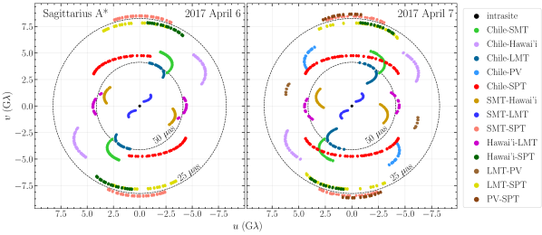
Figure 1: $(u,v)$-coverage of the EHT observations of Sgr A^∗ on 2017 April 6 and 7, from the HOPS dataset. Each point represents scan-averaged data, both bands are shown. “Chile” represents the stations ALMA and APEX. “Hawaiʻi” represents the stations SMA and JCMT. Dashed line circles indicate the fringe spacing of 50 $\mu$as and 25 $\mu$as.

2.3 Data Properties

2.3.1 General Aspects of Sgr A^∗ Data

The highly sensitive phased ALMA array participated in three of the five observing days, 2017 April 6, 7, and 11. April 7 is the only day that additionally includes PV observations of Sgr A^∗, and is therefore the day with the longest observation duration, largest number of detections, and the best overall $(u,v)$-coverage, as shown in Fig. 1. On April 11 an X-ray flare was reported shortly before the start of the EHT observations (Paper II). Strongly enhanced flux density variability is seen in the light curves on that day (Wielgus et al., 2022), possibly posing difficulties for the static imaging of the April 11 data set. These constraints motivate utilizing the less variable 2017 April 7 data as the primary data set for static image reconstruction, with the April 6 observations as a secondary validation data set. Analysis of the remaining 2017 EHT observations of Sgr A^∗ will be presented elsewhere.

In Fig. 1, the $(u,v)$-coverage on 2017 April 7 is shown to be asymmetric, with the longest baselines along the north-south direction. The shortest baselines in the EHT are intra-site and sensitive to arcsecond-scale structure (i.e., the SMA and JCMT are separated by 0.16  km; ALMA and APEX are separated by 2.6 km). In contrast, the longest baselines are sensitive to microarcsecond-scale structure (see Tab. 1). The $\sim 8.7$ G$\lambda$ detections on PV–SPT and SMT–SPT baselines are among the longest published projected baseline lengths obtained with ground-based VLBI, alongside the recent EHT 3C 279 results of Kim et al. (2020), slightly longer than the longest baselines in the EHT observations of M87* (8.3 G$\lambda$; M87^∗ Paper IV, ). Sgr A^∗ was detected on all baselines between stations with mutual visibility, leading to the April 7 $(u,v)$-coverage approaching the best one theoretically possible with the EHT 2017 array. Table 1 shows the angular resolutions derived from $(u,v)$-coverage on both April 6 and 7 data.

	${\rm FWHM}_{\rm maj}$	${\rm FWHM}_{\rm min}$	P.A.
	($\mu$as)	($\mu$as)	(∘)
Minimum Fringe Spacing $1/|\mathbf{u}|_{\rm max}$ (All Baselines)
April 6	24.2	—	—
April 7	23.7	—	—
Minimum Fringe Spacing (ALMA Baselines)
April 6-7	28.6	—	—
CLEAN Beam (Uniform Weighting)
April 6	24.8	15.3	67.0
April 7	23.0	15.3	66.6
CLEAN Restoring Beam (Used in This Paper)
April 6-7	20	20	—

Table 1: Metrics of EHT angular resolution for the 2017 observations of Sgr A^∗ for the 229.1 GHz band. In order to avoid asymmetries introduced by restoring beams, and to homogenize the images among epochs, we adopt a circular Gaussian restoring beam with $20\,\mu{\rm as}$ FWHM for all CLEAN reconstructions.

In the top panel of Fig. 2 we show in the signal-to-noise ratio of the Sgr A^∗ observations as a function of projected baseline length, for the coherent averaging time of 120 s. The split in S/N distributions at various projected baseline lengths is due to the difference in sensitivity for the co-located Chile sites ALMA and APEX, with ALMA baselines yielding detections stronger by about an order of magnitude. In the bottom panel, we show the visibility amplitude (correlated flux density in units of Jansky) for Sgr A^∗ as a function of projected baseline length after applying full data calibration.

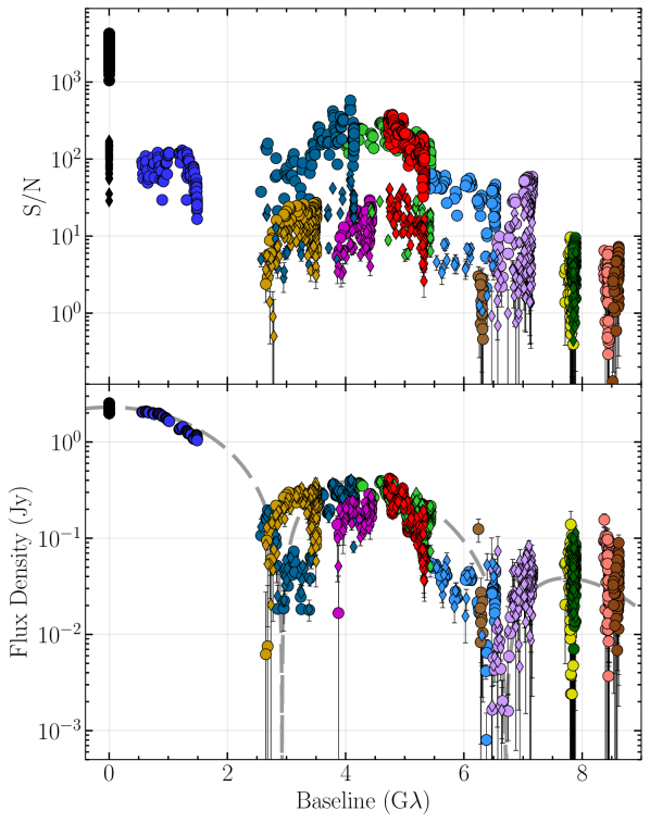
Figure 2: Top: signal to noise ratio (S/N) as a function of the $(u,v)$-distance (projected baseline length). Low band HOPS data recorded on 2017 April 7, averaged in 120 s segments, are shown. The data points are color-coded with the baseline, following Fig. 1. Bottom: fully calibrated visibility amplitude data. A model corresponding to a thin ring with a 54 $\mu$as diameter, blurred with a 23 $\mu$as FWHM circular Gaussian is overplotted for a reference (dashed curve).

The fully-calibrated visibility amplitudes exhibit a prominent secondary peak between two local minima. The first minimum is located at $\sim$3.0 G$\lambda$ and is probed by the Chile–LMT north-south baselines on 2017 April 7. On April 6 recording started about 2 h later, thus missing the relevant detections, as shown in Fig. 3. The second minimum appears at $\sim$6.5 G$\lambda$, probed by the Chile–Hawaiʻi baselines on both 2017 April 6 and 7. Overall amplitude structure of the source appears to be consistent across both days, which is particularly well visible in the fully-calibrated, light-curve-normalized data sets shown in Fig. 3, as the light-curve-normalization procedure strongly suppresses the large-scale source intrinsic variability (Broderick et al., 2022). The observed local visibility amplitude minima can be associated with the nulls of the Bessel function $J_{0}$, corresponding to the Fourier transform of an infinitely thin ring. For a ring that is 54 $\mu$as in diameter we would obtain local amplitude minima at 2.92 G$\lambda$ and 6.71 G$\lambda$. This is illustrated in the bottom panel of Fig. 2, where an analytic Fourier transform of an infinitely thin ring blurred with a 23 $\mu$as full width at half maximum (FWHM) Gaussian kernel is shown with dashed lines. While a blurred ring model roughly captures the dependence of visibility amplitudes on projected baseline length, there is also a clear indication of the source asymmetry, manifesting as amplitude differences between the Chile–LMT and SMT–Hawaiʻi baselines at the first minimum, probing the same range in projected baseline length ($\sim$2.5-3.5 G$\lambda$) in orthogonal directions. There is also a deficit of flux density with respect to the simple ring model at projected baseline lengths of $\sim$ 5-6 G$\lambda$.

Finally, we detect very clear and unambiguous non-zero closure phases, that are indicative of source asymmetry. With multiple independent triangles and high S/N, these data sets offer insight into the source phase structure greatly surpassing that of any previous mm-wavelength observations (Fish et al., 2016; Lu et al., 2018). In Fig. 4, we show examples of closure phases on several triangles exhibiting various degrees of probed asymmetry and inter/intra-day time variability. Closure phases on ALMA-SMT-SMA and ALMA-LMT-SMA triangles immediately show inter-day variability of the source structure. In the case of Sgr A^∗, intrinsic source variability is expected also on timescales as short as minutes, adding to the closure phase intra-day variability caused by the non-trivial average structure of the source (see Section 3.2). Very long baselines, such as LMT-SPT in the ALMA-LMT-SPT triangle, are additionally affected by the presence of refractive scattering structure (see Section 3.1).

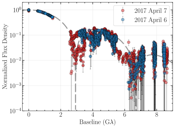
Figure 3: Comparison of the light-curve-normalized flux density measurements on 2017 April 6 and 7 in the fully calibrated HOPS data, averaged in 120 s segments and between low and high bands, are shown.

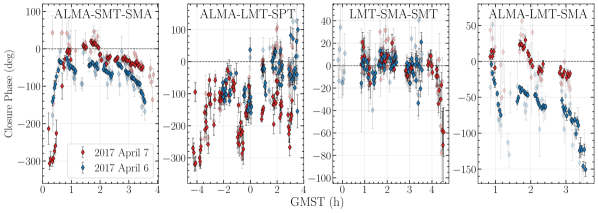
Figure 4: Examples of closure phases of Sgr A^∗, observed on 2017 April 6 and 7. Semi-transparent points correspond to measurements on redundant APEX/JCMT triangles. Data reduced with the HOPS pipeline, integrated in 120 s segments, averaged between both bands, are shown. No significant differences are seen with respect to the CASA-based calibration.

2.3.2 Station Gain Uncertainties and Non-closing Errors

Typically, the antenna gains and sensitivities as a function of elevation are derived using polynomial fits to opacity-corrected antenna temperature measurements from quasars and solar system objects, tracked over a wide range of elevations. Residual errors in the characterization of these antenna gains lead to corruptions in the flux calibration of the visibilities. Quantifying these effects enables us to disentangle astrophysical variability of Sgr A^∗ from apparent flux variations caused by the imperfect calibration. In this work, we mitigate the systematic gain errors in the Sgr A^∗ data sets based on the analysis of the calibrator sources (J1924-2914 and NRAO 530), that remained stationary in their source structure and flux density on relevant timescales. The detailed procedure to estimate the antenna gains from the two calibrators are described in section 5.1.3 in Paper II. In particular, it is shown that the a priori gains are 5-15% for all baselines, except intrasite baselines ($\sim 1\%$) and those including the LMT ($\sim 35\%$).

In addition to the thermal noise and the antenna gain uncertainties, we also estimate the non-closing errors in the data, based on deviations of the trivial closure quantities from zero, as well as from the observed inconsistencies in the distributions of closure quantities between bands and polarizations (; ). These non-closing errors are expected to arise from the presence of a small circular polarization component, as well as from uncorrected polarimetric leakages, and other systematic errors, such as residual bandpass effects. For Sgr A^∗, the non-closing errors are estimated to be 2° in closure phase and 8% in log closure amplitude (Paper II). Assuming the errors are baseline-independent, these translate to 1° systematic non-closing uncertainties in visibility phases and 4% systematic non-closing uncertainties in visibility amplitudes, on the top of the uncertainties related to the amplitude gains calibration. We found that the $RR-LL$ discrepancies in closure quantities are more significant for Sgr A^∗ than in the case of the calibrators. This hints at an intrinsic source property, possibly a contribution from a small circular polarization component. This is consistent with Goddi et al. (2021), reporting $\sim\,1\%$ circular polarization in the simultaneous ALMA-only data.

3 Mitigation of Scattering and Time Variability

The imaging of Sgr A* at 230 GHz with the EHT is challenged by two important effects: interstellar scattering and short-timescale variability. In this section, we introduce strategies for mitigating the effects of scattering (Section 3.1) and intrinsic variability (Section 3.2) adopted in this work.

3.1 Effects of Interstellar Scattering

Fluctuations in the tenuous plasma’s electron density along the line of sight causes scattering of the radio waves from Sgr A^∗. The scattering properties of Sgr A^∗ can be well described by a single, thin, phase changing screen $\phi(\textbf{r})$, where r is a two-dimensional vector transverse to the line of sight. The electron density fluctuation on the phase screen is typically characterized by a single power-law spectral shape between the outer ($r_{\rm out}$) and inner ($r_{\rm in}$) scale as $Q(\mathbf{q})\propto|\mathbf{q}|^{-\beta}$, where $\mathbf{q}$ is the wavevector of the propagating radio wave and a Kolmogorov spectrum of density fluctuations gives $\beta=11/3$ (Goldreich & Sridhar, 1995). The statistical effects of the scattering can then be related to a spatial structure function $D_{\phi}(\mathbf{r})=\left<[\phi(\mathbf{r}+\mathbf{r_{0}})-\phi(\mathbf{r_{0}})]^{2}\right>_{\mathbf{r_{0}}}\propto\lambda^{2}$, where $\left<\cdot\right>_{\mathbf{r_{0}}}$ denotes the ensemble average over $\mathbf{r_{0}}$.

The interstellar scattering of radio waves from Sgr A^∗ is in the regime of strong scattering, where scintillation is dominated by two distinct effects, diffraction and refraction, attributed to widely separated scales (see Narayan, 1992; Johnson & Gwinn, 2015). Diffractive scintillation arises from fluctuations on the scale of the phase coherence (or diffractive scale) given by $D_{\phi}(\textbf{r})\sim 1$. It causes rapid temporal variations on a time scale much shorter than 1 s for Sgr A^∗, which is also much shorter than the integration time of radio observations. As a result, radio observations measure ensemble averages of the diffractively scattered structure, appearing as the intrinsic structure blurred with the scattering kernel (see Section 3.1.1).

Refractive scintillation arises from fluctuations on the scale of the scattering kernel much larger than the phase coherence length in the strong scattering regime. For Sgr A^∗, the refractive scintillation causes temporal variations of the source images over a time scale of $\sim 1$ d at 1.3 mm (e.g. Johnson et al., 2018) – longer than the typical length of radio observations including our EHT observations. Consequently, a single realization of refractive scintillation will be observed by the EHT over an observing run; this will appear as an angular-broadened (i.e., diffractively-scattered) source structure with compact substructure caused by refractive scintillation (Narayan & Nityananda, 1986a; Johnson & Gwinn, 2015; Johnson & Narayan, 2016).

A brief introduction of the expected scattering properties in the EHT 2017 data is described in Section 5.1 of Paper II. Here we describe the scattering mitigation strategy for the effects of angular broadening by diffractive scattering (Section 3.1.1) and substructure induced by refractive scattering (Section 3.1.2). To describe scattering effects on Sgr A^∗, we use a theoretical framework of these scattering effects developed by Psaltis et al. (2018), whose model parameters have been observationally studied by Johnson et al. (2018), Issaoun et al. (2019, 2021) and Cho et al. (2022). For general background and reviews on interstellar scattering, see Rickett (1990), Narayan (1992), or Thompson et al. (2017).

3.1.1 Mitigation of Angular Broadening

Angular broadening is described by a convolution of an unscattered image with a scattering kernel, or equivalently by a multiplication of unscattering interferometric visibilities by the appropriate Fourier-conjugate kernel. The Fourier-conjugate kernel is given by $\exp\left[-\frac{1}{2}D_{\phi}{(\mathbf{b}/(1+\mathcal{M}))}\right]$, where $\mathbf{b}$ is the baseline vector of the interferometer and $\mathcal{M}$ is the magnification of the scattering screen given by the ratio of the observer-to-screen distance to the screen-to-source distance. Interferometric measurements of Sgr A^∗ with the EHT at the observing wavelength of 1.3 mm are primarily obtained on long baselines of $|\textbf{b}|\mathrel{\raise 1.29167pt\hbox{$>$\kern-7.5pt\lower 4.30554pt\hbox{$\sim$}}}(1+\mathcal{M})r_{\rm in}$, or equivalently on angular scales of $\theta\lesssim\lambda/(1+\mathcal{M})r_{\rm in}$, where $r_{\rm in}$ is the inner scale of the fluctuations. In this regime, the angular broadening is affected by the power-law density fluctuations on scales between the inner and outer scales, giving the phase structure function of $D_{\phi}(\mathbf{r})\propto\lambda^{2}|\mathbf{r}|^{-\alpha}$, where $\alpha=\beta-2$.

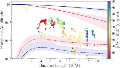
Figure 5: Projection of the diffractive scattering kernel (solid lines) and flux-normalized refractive noise amplitudes (dashed lines) at 1.3 mm based on the scattering model of Johnson et al. (2018), overlaid on light-curve-normalized Sgr A^∗ data (low band on April 7). The red and blue lines correspond to the major and minor axes of the scattering, respectively. The associated shaded area indicates the 3$\sigma$ uncertainty of the scattering model in Johnson et al. (2018). Sgr A^∗ data are colored by their position angle difference from the major axis of the scattering kernel — as the points change from red to blue the $(u,v)$ coordinates move from being closer to the major to minor scattering axis. Regardless of the position angle, Sgr A^∗ amplitudes appear to more rapidly decrease than the scattering kernel, indicating that the intrinsic structure is well resolved against the diffractive angular broadening effects. Additionally, most Sgr A^∗ amplitudes are above the refractive floor. Thus, refractive effects should only dominate for a small amount of data above $\sim 6\,\mathrm{G}\lambda$.

In Figure 5, we show the scattering kernel in the visibility domains based on the scattering parameters in Johnson et al. (2018). Johnson et al. (2018) imply a near-Kolmogorov power-law spectral index $\beta\sim 3.38$ (or $\alpha\sim 1.38$), providing a non-Gaussian kernel more compact than the conventional Gaussian kernel. Consequently, the angular broadening effect, i.e. multiplication of the intrinsic visibilities with the Fourier-conjugate kernel of scattering, causes a slight decrease in visibility amplitudes and therefore also the S/N by a factor of a few at maximum.

Angular broadening provides deterministic and multiplicative effects on the observed visibility. Therefore, it is invertible — they can be mitigated by dividing the observed visibility and associated uncertainties by the diffractive kernel visibility (often called deblurring; Fish et al., 2014). However, the actual interferometric measurements of Sgr A^∗ with the EHT have contributions from substructure that arises from the refractive scattering, often referred as the “refractive noise.” The refractive noise is stochastic and additive, and therefore not invertible (Johnson & Narayan, 2016). In fact, since refractive effects are included in the diffractively blurred image, the refractive noise will be amplified by simply deblurring with the scattering kernel, and likely create artifacts in the reconstructions if not accounted for (Johnson, 2016). To avoid effects from refractive noise we expand the noise budgets of the visibility data prior to deblurring, as described in Section 3.1.2.

3.1.2 Mitigation of Refractive Scattering

The contribution of the refractive noise to the observed visibility is anticipated to be not dominant, except for a small fraction of data beyond $\sim 6\,G\lambda$ (Figure 5). Signature of the refractive noise, namely the long, flat tail of the visibility amplitude at long baselines found in recent longer wavelength observations of Sgr A^∗ (Johnson & Gwinn, 2015; Johnson et al., 2018; Issaoun et al., 2019, 2021; Cho et al., 2022) is not clearly seen in the EHT data. In this EHT regime, where the refractive substructure is not unambiguously constrained from data, it is challenging to apply complex strategies that account for the stochastic properties or explicitly recover the refractive screen (e.g. Johnson, 2016; Johnson et al., 2018; Issaoun et al., 2019; Broderick et al., 2020a).

We instead mitigate the effect of refractive substructure by introducing error budget models that approximate the anticipated refractive noise. The visibility error budget is increased based on these models prior to the mitigation of angular broadening via deblurring (Section 3.1.1). In this work, we consider four base models that approximate the refractive noise budgets: i. Const: a constant noise floor (e.g., $10\,$mJy) for all baselines motivated by the fact that the refractive noise has a mostly flat profile as a function of the baseline length (see Figure 5), ii. J18model1: $(u,v)$ dependent noise floor based on the scattering model and parameters described in Psaltis et al. (2018) and Johnson et al. (2018). Since the scattered image is not unique, we have simulated hundreds of scattering realizations and generated corresponding synthetic data that matches the $(u,v)$-coverage of the actual April 7 observation of Sgr A^∗. The refractive noise values are then computed by taking the standard deviation of the complex visibilities across different realizations. Since the refractive noise is also dependent on the intrinsic source structure, in this case we consider a circular Gaussian model with the 2nd moment that matches the pre-imaging size constraints (see Paper II), iii. J18model2: Same as J18model1 but using the average refractive noise value of seven geometric models as possible intrinsic source structures (see Section 5), iv. considering not only the standard deviation of the refractive effects, but their correlations via a covariance matrix as well.

Note that using all the information encoded in the covariance matrix (not only in the variance of the refractive noise variables) will provide a better approximation of the refractive noise. However, the short time cadence and the redundant baselines in our data make this covariance matrix non-invertible, and thus difficult to use in imaging. For the remaining three refractive noise models, we compute the complex visibility $\chi^{2}$ for a suite of synthetic data (corrupted only by thermal noise along with scattering effects) based on seven geometric models of the intrinsic source structure (Section 5),

$$\chi^{2}\left(\sigma_{\mathrm{ref,i}}\right)=\frac{1}{2N_{\mathrm{vis}}}\sum_{\mathrm{i=1}}^{N_{\mathrm{vis}}}\frac{\lvert V_{\mathrm{i}}-V_{\mathrm{ea}}\rvert^{2}}{\sigma_{\mathrm{th,i}}^{2}+\sigma_{\mathrm{ref,i}}^{2}},$$ (1)

where $V_{i}$ is the data visibilities for each scattering realization, $V_{ea}$ is the ensemble averaged visibilities (i.e., corresponding to the image experiencing only diffractive scattering), $\sigma_{\mathrm{th,i}}$ is the thermal noise, and $\sigma_{\mathrm{ref,i}}$ is the corresponding refractive noise budget for each strategy. The $\chi^{2}$ metric provides us with a statistic on how well the ensemble average image represents the synthetic data after taking into account the different modeled refractive noise budgets. Figure 6 shows a comparison of the different $\chi^{2}$ distributions for 400 realizations of synthetic data for every scattering mitigation strategy. For J18model1 we have derived a scaling factor to make the median of $\chi^{2}$ of all models equal to 1 in order to overcome the dependence of the refractive noise level on the intrinsic source structure (see Appendix B).

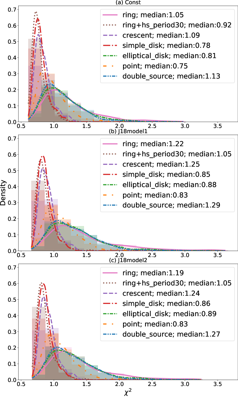
Figure 6: Reduced $\chi^{2}$ distributions and their density function (in solid lines) for all geometric models of intrinsic source structure using the three different refractive noise models (Const, J18model1 and J18model2). For all noise models, the majority of the $\chi^{2}$s falls in the range between 0.5 and 2.0 (ideally $\chi^{2}=1.0$), which indicates the ensemble average images provide reasonable fits to the simulated data after taking into account one of the proposed refractive noise budgets.

Figure 6 demonstrates that the (Const, J18model1, and J18model2) refractive noise models result in reasonable $\chi^{2}$s for the simulated scattering realizations we tested, with a majority of the $\chi^{2}$ values below 3.0 (ideally $\chi^{2}=1$). For this reason, in the rest of the paper we focus on the simpler Const and J18model1 strategies.

3.2 Effects of Time Variability

With a gravitational timescale of only $GM/c^{3}\approx$ 20 s, Sgr A^∗ is expected to be able to exhibit substantial changes in its emission structure on timescales of a few minutes or less. A single multi-hour observing track is thus sufficiently long for Sgr A^∗ to significantly alter its appearance, potentially hundreds of times. Such structural variability violates a core assumption of Earth-rotation aperture synthesis – namely, that the source structure must remain static throughout the observation – and necessitates modifications to standard imaging practices.

3.2.1 Evidence for Source Variability in the Data

The EHT Sgr A^∗ data contain unambiguous signatures of an evolving emission structure. On the largest spatial scales, the light curve varies at the $\sim$10% level on timescales of $\sim$hours (Wielgus et al., 2022). Variations in excess of those expected from thermal noise are seen on timescales as short as $\sim$1 min. Over timescales typical of observation scans, $\sim$10 min, the degree of variation is on the order of 5% (Wielgus et al., 2022).

Direct evidence for short-timescale structural variations may be found in the evolution of closure quantities. Closure phases measured on certain triangles of baselines (e.g., ALMA-SMT-SMA) exhibit significant differences between April 6 and 7 (see Figure 4). The variations seen in the closure phases measured on multiple triangles show significant excesses, relative to thermal noise levels, as captured using the $\mathcal{Q}$-metric statistic (Roelofs et al. 2017, Paper II).

Non-parametric estimates of the degree of variability as a function of baseline length may be generated by inspecting the visibility amplitudes directly. This is made possible by two fortuitous facts: first, the existence of crossing tracks, and second, that Sgr A^∗ was observed on multiple days. As a result, many presumably independent realizations of the source structure may be compared. Practically, this is obtained by collecting visibility amplitudes in $(u,v)$ bins, linearly detrending to remove the contribution from the static component of the image, and computing the mean and variance of the residuals. We average these estimates azimuthally to improve the significance of variability detection. For details on the procedure and validation examples, we direct the reader to Georgiev et al. (2021) and Paper IV.

In the case of Sgr A^∗, this non-parametric estimate produces a clear detection of variability that is significantly in excess of the expected thermal noise (Paper IV). Within the range of baseline lengths over which meaningful estimates can be produced, roughly $2~{}{\rm G}\lambda<|u|<6~{}{\rm G}\lambda$, the observed excess variability is broadly consistent with that anticipated by GRMHD simulations, both in magnitude and dependence upon baseline length (; ).

3.2.2 Strategies for Imaging Variable Data

Strategies for imaging in the face of source variability can be classified into one of three general categories:

1. Variability reconstruction, or “dynamic imaging,” in which the evolution of the source emission structure is explicitly recovered during the imaging process. The output of this strategy is a movie of the source emission structure. We refer the reader to Section 4.4 for more discussion on methods for dynamic imaging.

2. Variability circumvention, or “snapshot imaging,” in which standard image reconstruction is performed on segments of data (“snapshots”) that are sufficiently short that the source may be approximated as static across them. The output of this strategy is a time series of static images.

3. Variability mitigation, or “variability noise modeling,” in which the impact of structural changes in the visibilities is absorbed into an appropriately inflated error budget. The output of this strategy is a single static image of the source, indicative of the time-averaged image over this observation period.

In practice, for segments of data short enough that Sgr A^∗ may be reasonably approximated as static, the $(u,v)$-coverage of the EHT is insufficient to support reliable snapshot image reconstruction (though more restrictive parameterizations of the source structure, such as permitted using geometric modeling, can still be applied; see Section 9 and Paper IV). However, because dynamic imaging enforces a degree of temporal continuity, it is able to leverage the information provided by densely-covered intervals of time to augment the lack of information available during intervals of sparser coverage. Dynamic imaging can thus be thought of as a generalization of both standard (static) imaging and snapshot imaging, with the former being equivalent to dynamic imaging with maximal temporal continuity enforcement and the latter being equivalent to dynamic imaging with no temporal continuity enforcement at all. Because dynamic imaging falls in between these two extremes, it can potentially recover reliable source structure in regions where the data are both too variable for standard imaging and too sparse for snapshot imaging. Our efforts to perform dynamic imaging in the most densely $(u,v)$-covered regions of data are described in Section 9.

The third strategy listed above – the variability noise modeling approach – permits static images to be reconstructed even from time-variable data. Depending on the specifics of the implementation, the recovered image captures some representation of “typical” source structure. Imaging with variability noise modeling requires that the error budget of the data be first inflated in a way to capture the statistics – or “noise” – of the source variability. The specific form of the noise model we use in this work is a broken power law, for which the variance $\sigma^{2}_{\text{var}}$, as a function of baseline length $|u|$, takes the form

$$\sigma_{\text{var}}^{2}(|u|)=a^{2}\left(\frac{|u|}{4~{}\text{G}\lambda}\right)^{c}\frac{1+\left[(4~{}\text{G}\lambda)/u_{0}\right]^{b+c}}{1+\left(|u|/u_{0}\right)^{b+c}}.$$ (2)

Here, $|u|\equiv\sqrt{u^{2}+v^{2}}$ is the dimensionless length of the baseline located at $(u,v)$, $u_{0}$ is the baseline length corresponding to the break in the power law, $a$ is the variability noise amplitude at a baseline length of 4 G$\lambda$, and $b$ and $c$ are the long- and short-baseline power-law indices, respectively. Equation 2 represents the variance that is associated with structural variability after removing the mean and normalizing by the light curve; see Paper IV for details.

By adding the variability noise given by Equation 2 in quadrature to the uncertainty of every visibility data point, the image becomes constrained to fit each data point to only within the tolerance permitted by the expected source variability. This parameterized variability noise model is generic and can explain well a wide range of source evolution, including complicated physical GRMHD simulations of Sgr A^∗ (Georgiev et al., 2021).

Paper IV presents a non-parametric analysis of Sgr A^∗’s variability, which is further inspected to provide ranges of broken-power-law model parameters that fit Sgr A^∗ data (see Georgiev et al., 2021, for details). As explained in Paper IV, given the baseline coverage of the 2017 Sgr A^∗ campaign, little traction is found on the location of the break, $u_{0}$, and the short-baseline power law, $c$. However, the amplitude $a$ is well constrained with an interquartile range from 1.9% to 2.1%. Similarly, the long-baseline power law, $b$, is modestly constrained, with interquartile range 2.2 to 3.2. These interquatile ranges are used to provide approximate priors on the variability noise that should be considered during static imaging reconstruction; values employed are listed in Table 2 for Sgr A^∗ as well as for a number of synthetic data sets described in Section 5. In the case of the later, theoretical considerations imply that under very general conditions, $c\approx 2$, and thus we adopt a general prior of $[1.5,2.5]$. For the CLEAN (Section 4.1) and regularized maximum likelihood (RML) (Section 4.2) imaging surveys described in Section 6, variability noise models in the identified Sgr A^∗ range are added to the visibility noise budget before static imaging (for both synthetic and real Sgr A^∗ data). For the Themis imaging method (Section 4.3), the parameters of the noise model are fit simultaneously with the image structure, subject to the data-set-specific values in Table 2 being used to define a uniform prior over each data set.

Table 2: Variability Noise Model Ranges used for Static Imaging

Source	$a$ (%)	$b$	$u_{0}$ (${\rm G}\lambda$)
Sgr A∗	$[1.9,2.1]$	$[2.2,3.2]$	$[0.37,1.45]$
Ring	$[0.7,0.8]$	$[1.9,3.0]$	$[0.18,1.06]$
Ring+hs	$[0.6,0.7]$	$[3.0,4.1]$	$[0.33,0.90]$
Crescent	$[0.9,1.1]$	$[2.4,3.4]$	$[0.29,1.15]$
Simple Disk	$[0.6,0.7]$	$[2.3,3.3]$	$[0.18,0.82]$
Elliptical Disk	$[0.6,0.7]$	$[2.1,3.0]$	$[0.16,0.77]$
Point	$[0.8,0.9]$	$[1.8,3.1]$	$[0.32,2.67]$
Double	$[0.8,0.9]$	$[1.9,2.9]$	$[0.19,1.09]$
GRMHD	$[2.4,2.7]$	$[2.6,3.8]$	$[0.56,1.78]$

4 Imaging Methods for Sgr A^∗

Recovering an image of Sgr A^∗ from interferometric measurements amounts to solving an inverse problem. This inverse problem is challenging because of four primary reasons: 1) the interferometer incompletely samples the visibility domain, 2) there is significant structured noise included in the visibility measurements, 3) the source structure is evolving over the duration of the observation, and 4) the source is both diffractively and refractively scattered. The methods used in M87^∗ Paper IV to recover an image of M87^∗ from interferometric measurements had to address challenges 1 and 2 above; challenges 3 and 4 are unique to the rapidly evolving Sgr A^∗ source, which we observe through the interstellar medium. Strategies to mitigate the effects of scattering and time variability are discussed in detail in Section 3. In this section we assume that the data have already been modified by the appropriate descattering strategy and variability noise budget prior to imaging.

To choose among the possible Sgr A^∗ images, additional information, assumptions, or constraints must be included when solving the inverse problem. We broadly categorize imaging algorithms into three methodologies: CLEAN, regularized maximum likelihood, and Bayesian posterior sampling. We summarize these approaches, but refer the reader to M87^∗ Paper IV for a more complete discussion of static imaging methods for EHT data. Additionally, we introduce the idea of dynamic imaging, which aims to reconstruct a movie rather than a single static image over an observation.

4.1 CLEAN Static Imaging

Traditionally, radio interferometric images have been made using non-linear deconvolution algorithms of the CLEAN family (e.g., Högbom, 1974; Schwarz, 1978; Clark, 1980; Schwab, 1984; Cornwell et al., 1999; Cornwell, 2008). These algorithms iteratively deconvolve the effects of the limited sampling of the $(u,v)$ plane, i.e., the interferometer’s point source response (also known as dirty beam) from the inverse Fourier transform of the visibilities (dirty image).

The classical CLEAN algorithm assumes that the sky brightness distribution can be represented as a collection of point sources. The imaging process consists of rounds of locating the brightness peak in the dirty image, generating a point source (CLEAN component) at this location with an intensity of some fraction of the map peak, and either convolving the CLEAN component with the dirty beam and subtracting it from the dirty image (Högbom, 1974; Clark, 1980) or subtracting the CLEAN components directly from the ungridded visibilities (Schwab, 1984). This is continued until some specified cleaning stopping criterion is reached. One can supplement the process by restricting the area in which the peaks are searched (so-called CLEAN windows). This limits the parameter space in fitting and is especially important for data with sparse $(u,v)$ sampling. The final image is made by convolving the obtained set of CLEAN components with a Gaussian restoring beam to smooth out the higher spatial frequencies and adding the last residual image to represent the remaining noise.

After image deconvolution, further improving of the image quality can be achieved using self-calibration, which uses the current image estimate to apply a correction to amplitude and phase information. Self-calibration is usually applied as part of an iterative process following each CLEAN iteration.

In this work we implement the CLEAN method using the DIFMAP pipeline described in Section 6 and Appendix D.1.

4.2 RML Static Imaging

The general approach in Regularized Maximum Likelihood static imaging methods is to find an image, $\hat{I}$, that minimizes a specified objective function. As described further in M87^∗ Paper IV, by using $\chi^{2}\left(I,V\right)$ as a measure of the inconsistency of the image, $I$, with the measurements, $V$, we can specify the objective function:

$$J(I)=\sum_{\mathclap{\text{data terms}}}\alpha_{\textrm{D}}\chi^{2}_{\textrm{D}}\left(I,V\right)-\sum_{\mathclap{\text{regularizers}}}\beta_{\textrm{R}}S_{\textrm{R}}\left(I\right).$$ (3)

In this expression, the $\chi^{2}_{\textrm{D}}$’s are goodness-of-fit functions corresponding to the data product $D$, and the $S_{\textrm{R}}$’s are regularization terms corresponding to the regularizer $R$. Maximum entropy (Narayan & Nityananda, 1986b; Chael et al., 2016), total variation, and sparsity priors (Wiaux et al., 2009a, b; Honma et al., 2014; Akiyama et al., 2017a) have all been used to define $S_{\textrm{R}}(I)$ and have been demonstrated in the interferometic imaging of M87^∗ (M87^∗ Paper IV). The $\chi^{2}_{\textrm{D}}(I,V)$ and $S_{\textrm{R}}(I)$ terms often have different preferences for the “best” image, and compete against each other in minimizing $J(I)$. Their relative impact in this minimization process is specified with the hyperparameters $\beta_{\textrm{R}}$.

This expression can be interpreted probabilistically when $\exp\left(-\sum\alpha_{\textrm{D}}\chi^{2}_{\textrm{D}}\left(I,V\right)\right)\propto p(V|I)$ and $\exp\left(\sum\beta_{\textrm{R}}S_{\textrm{R}}\left(I\right)\right)\propto p(I)$. In this case, minimizing the cost function $J(I)$ is equivalent to maximizing the log-posterior $\log p(I|V)$. Not all regularizer cost functions $S_{\textrm{R}}$ correspond to a formal probability distribution. Nonetheless, while not all RML methods have a probabilistic interpretation, their formulation leads to a similar optimization setup.

For the EHT, RML methods have an advantage of being able to naturally constrain closure data products that are insensitive to atmospheric noise that corrupts EHT visibilities (Bouman et al., 2016; Chael et al., 2016; Akiyama et al., 2017a; Chael et al., 2018). In this work we implement RML methods using the eht-imaging and SMILI pipelines described in Section 6 and Appendices D.2 and D.3.

4.3 Bayesian Full Posterior Static Imaging

A fully Bayesian approach to imaging is a natural extension of the RML approach to image reconstruction. The primary output of Bayesian methods is an image posterior, i.e., not only a single “best fit” image but the family of images that are consistent with the underlying visibility data. In this way, the Bayesian image posterior encapsulates both the typical image reconstruction and its aleatoric (e.g., statistical) uncertainty, permitting quantitative analyses of the robustness of image features, array calibration quantities, and the relationships between each (see, e.g., Broderick et al. 2020b; Arras et al. 2019; Sun & Bouman 2021; Pesce 2021; M87^∗ Paper VII).

We employ the general modeling framework Themis, developed specifically to compare parameterized models with the VLBI data produced by the EHT (Broderick et al., 2020a). The image model consists of three conceptually distinct components: a description of the brightness distribution on the sky, the variable complex gains at each station, and the additional “noise” associated with intra-day structural variability in the source. Scan-specific complex station gains and variability “noise” parameters are recovered and marginalized over simultaneously with image exploration. Details on the model construction, adopted priors, sampling methods, and fidelity criteria are collected in Appendix A, and are only briefly summarized here.

We make use of the adaptive splined raster models within Themis, consisting of a set of brightness control points that may vary in brightness on an adjustable rectilinear grid. In practice, only a handful of resolution elements are required (see Section 6.3 and Section D.4), and full images are produced via an approximate cubic spline (Broderick et al., 2020b). The dimensions of the raster, $N_{x}$ and $N_{y}$, are selected based upon the Bayesian evidence as discussed further in Section 6.3.

The combined parameter space, comprised of the brightness control points, raster size and orientation, complex station gains, and noise model parameters are sampled via a parallely tempered, Hamiltonian Monte Carlo scheme, producing a chain of candidate images and ancillary quantities that are distributed according to their posterior probability, $p(I|V)$. In practice, the sampler must explore the parameter space sufficiently to produce an accurate reproduction of the posterior, often referred to as “convergence,” which we assess via standard convergence criteria. A fully converged Markov chain will have identified all available image modes that can be captured by the specified image representation, and assessed their relative likelihoods.

4.4 Dynamic Imaging

As discussed in Section 3.2.2, the quickly evolving structure of Sgr A^∗ poses significant challenges in reconstructing an image. Imaging techniques traditionally rely on Earth rotation aperture synthesis, which are based on the fundamental assumption that the target being imaged remains stationary during the whole duration of the observation. This is no longer valid when the target source is expected to exhibit significant structural changes in time scales smaller than the observing run; thus for static imaging we must incorporate an inflated “variability noise budget" to capture the “typical" source structure (refer to Section 3.2.2). If we instead wish to capture the evolving structure of Sgr A^∗ we can attempt to recover a full movie from the data, rather than just a single image.

Extensions of the CLEAN approach have been proposed to address time-variable sources Stewart et al. (2011); Rau (2012); Farah et al. (2021). In Miller-Jones et al. (2019) evolution of the microquasar V404 Cygni was reconstructed using model fitting in DIFMAP. Arras et al. (2019) developed a variational inference approach for dynamic imaging that was used to simultaneously reconstruct images of M87^∗ over four nights from EHT 2017 data. In this work we focus on methods that explicitly incorporate temporal regularization to allow for recovery of evolving sources with complex spatial structure in the presence of especially sparse $(u,v)$-coverage.

4.4.1 RML Dynamic Imaging

Extending the RML approach from static to dynamic imaging is simple conceptually. Rather than solving for a single image, $\hat{I}$, our new goal is to solve for a series of $K$ images $\hat{\{I_{k}\}}$. Each of these images correspond with small segments of data, which have been divided to have a time duration similar to the expected time variability of the target (typically tens of minutes for Sgr A^∗). Since the $(u,v)$-coverage of each data segment is severely limited, we must include an additional term that regularizes the images ${\{I_{k}\}}$ in time rather than just space. A general prescription in terms of the temporal regularizer $S_{\textrm{Q}}$ can be written mathematically as:

$$J(\{I_{k}\})= \sum_{\mathclap{\text{data terms}}}\alpha_{\textrm{D}}\chi^{2}_{\textrm{D}}\left(\{I_{k}\},V\right)$$

$$-\sum_{\mathclap{\text{spatial reg.}}}\beta_{\textrm{R}}S_{\textrm{R}}\left(\{I_{k}\}\right)-\sum_{\mathclap{\text{temporal reg.}}}\beta_{\textrm{Q}}S_{\textrm{Q}}\left(\{I_{k}\}\right).$$ (4)

The additional temporal regularization terms, $S_{\textrm{Q}}$, encourages smooth evolution of the target over the full observation. Descriptions of temporal regularizers and their application to EHT data are described in Johnson et al. (2017).

In Appendix G the RML Dynamic Imaging method is used to explore the structure of Sgr A^∗ over the course of a night independent of the variability noise model introduced in Section 3.2.2.

4.4.2 StarWarps Dynamic Imaging

StarWarps is a dynamic imaging method based on a probabilistic graphical model (Bouman et al., 2018). Similar to RML Dynamic Imaging, StarWarps makes use of temporal regularization to solve for the frames of a movie $\hat{\{I_{k}\}}$ over an observation rather than a static image. In contrast to RML, StarWarps independently solves for the marginal posterior of each frame conditioned on all measurements in time; the reconstructed movie $\hat{\{I_{k}\}}$ is the mean of each marginal distribution. The advantage of StarWarps with respect to RML is that, when using a linearized measurement model, StarWarps can solve for the frames of a video $\hat{\{I_{k}\}}$ with exact inference – resulting in a better behaved optimization problem that is less likely to get stuck in local minima when compared to RML Dynamic Imaging.

StarWarps defines a dynamic imaging model for observed data using the following potential functions:

$$\psi_{V_{k}|I_{k}} =\mathcal{N}_{V_{k}}(f_{k}(I_{k}),\sigma_{k}^{2})$$ (5)

$$\psi_{I_{k}} =\mathcal{N}_{I_{k}}(\mu,\Lambda)$$ (6)

$$\psi_{I_{k}|I_{k-1}} =\mathcal{N}_{I_{k}}(I_{k-1},\beta_{Q}^{-1}\mathbbm{1}),$$ (7)

for a normal distribution $\mathcal{N}(m,C)$ with mean $m$ and matrix covariance or scalar standard deviation $C$. Each set of observed data $V_{k}$ taken at time $k$ is related to the underlying image, $I_{k}$, through the measurement model, $f_{k}(I_{k})$ (e.g., visibility model, closure phase model). Spatial regularization is imposed through the second potential; $I_{k}$ is encouraged to be a sample from a multivariate Gaussian distribution with mean $\mu$ and covariance $\Lambda$. In this work, we define $\Lambda$ to encourage spatial smoothness with a spectral distribution profile $(u^{2}+v^{2})^{-a/2}$ controlled by hyperparameter $a$, as described in detail in Bouman et al. (2018). The third potential describes how images evolve over time; as $\beta_{Q}$ increases the temporal regularization increases and visa versa. Although more complex evolution models are described in Bouman et al. (2018), in this paper we restrict ourselves to a simplified evolution model that encourages only small changes between adjacent frames $I_{k-1}$ and $I_{k}$.

The joint probability distribution of this dynamic model can be written as:

$$p(\{I_{k}\},\{V_{k}\})=p(I_{1})\prod_{k=1}^{K}p(V_{k}|I_{k})\prod_{k=2}^{K}p(I_{k}|I_{k-1})$$ (8)

where $p(I_{1})=\psi_{I_{1}}$, $p(V_{k}|I_{k})=\psi_{V_{k}|I_{k}}$, and $p(V_{k}|I_{k})\propto\psi_{I_{k}}\psi_{I_{k}|I_{k-1}}$. In the case of a linear measurement model, $f(I)$, (e.g., complex visibility model) the expected value of every $I_{k}$ conditioned on all data $V=\{V_{k}\}$ can be solved in closed-form efficiently using the Elimination Algorithm. However, in the case of complex gain errors the measurement model is no longer linear. By linearizing the model we can solve in closed form for a linearized solution, $\hat{\{I_{k}\}}$. We then iterate between linearizing the measurement model around our current solution and solving the linearized solution in closed-form until convergence.

The StarWarps method is used in Section 9 alongside snapshot geometric modeling methods to help analyze the short-timescale variations of Sgr A^∗ over a $\sim 100$ min region of time on April 6 and 7.

5 Synthetic Data

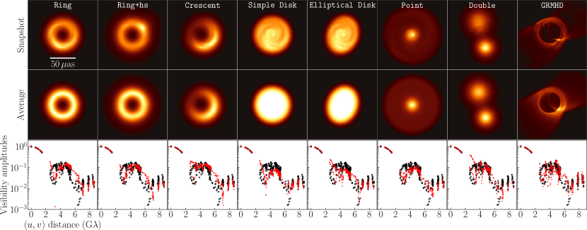
Figure 7: Eight synthetic models and corresponding visibility amplitudes. From left to right, we show the seven geometric models and the single GRMHD model. Top panels: a single frame of the eight synthetic movies highlighting the effect of temporal variability. Middle panels: time-averaged images illustrating the static component of the source structure. Bottom panels: a comparison of the simulated visibility amplitudes (red) and real Sgr A^∗ measurements (black) as a function of projected baseline length.

While imaging is a powerful tool to identify the source morphology without a specific source model, reconstructed images obtained with the techniques described in Section 4 are sensitive to hyper-parameter and optimization choices (in this paper, often referred to simply as parameter choices). For instance, in RML imaging methods, a common design choice is the type of regularizers and how much weight to assign the regularization terms relative to data fitting terms. In CLEAN, common design choices include the location of CLEAN windows and the initial model used for self-calibration. Reconstructed images can be sensitive to these choices, especially when the data constraints are severely limited, as is the case in the sparse EHT measurements of Sgr A^∗.

In the second half of 2019, images of Sgr A^∗ were initially reconstructed by five teams that worked independently of each other to identify the morphology of Sgr A^∗ through imaging. As summarized in Appendix C, the five independent teams identified a $\sim$50 $\mu$as feature, but with a significant uncertainty in the detailed morphology. While many of the images contained a ring structure, some of the teams obtained non-ring images that also reasonably fit the data. Furthermore, the flux distribution around the recovered rings showed large variation across different reconstructions. These initial images motivated a series of tests presented in this paper to systematically study the possible underlying source structure of Sgr A^∗.

To systematically explore and evaluate the imaging algorithms design choices and their effects on the resulting image reconstructions, we generated a series of synthetic data sets. The synthetic data were carefully constructed to match properties of Sgr A^∗ EHT measurements. The use of synthetic data enables quantitative evaluation of image reconstruction by comparison to the known ground truth. This in turn enables evaluation of the design choices and imaging algorithms performance (Section 4). As summarized in Figure 7 two sets of time-variable synthetic data were generated for slightly different purposes. The first set are the geometric models (Section 5.1), which were used to both assess the capability of identifying and distinguishing different morphologies as well as to select optimal design choices and parameters (for RML and CLEAN) that perform well across the entire data set. The second data set is the GRMHD model which was used to evaluate imaging performance on physically motivated models of Sgr A^∗ (see Section 6).

Data sets were generated using eht-imaging’s simulation library with a $(u,v)$-coverage identical to Sgr A^∗ measurements. Prior to the synthetic observations, all movies were scattered based on the best-fit model of Johnson et al. (2018) (see Section 3.1 for details). The observed visibilities were further corrupted by thermal noise, amplitude gains, and polarization leakage, consistent with Sgr A^∗ data (Paper II). Atmospheric phase fluctuations were simulated by randomizing the visibility phase gains on a scan-by-scan basis.

5.1 Geometric Models

To assess the capability of identifying source morphology, seven geometric models were used to generate synthetic data (Figure 7). As described in Section 5.1.1, the time-averaged morphology of these models was motivated by the first imaging results (Appendix C). Furthermore, the geometric model parameters were adjusted and selected to be qualitatively consistent with Sgr A^∗ measurements. To assess the effects of temporal variability on the reconstructed images, a dynamic component is added to the time-averaged models. The static geometric models are modulated by an evolution generated statistical model with parameters optimized to match metrics seen in Sgr A^∗ data.

5.1.1 Time-averaged Morphology

We use the following three ring models motivated by the morphology identified in many “first images" presented in Appendix C: symmetric and asymmetric ring models (henceforth Ring and Crescent, respectively) and a symmetric ring model with a bright hot spot that rotates in the counter-clock-wise direction with a period of 30 min (henceforth Ring+hs). The first two models are designed to test whether our imaging methods can identify a symmetric vs. asymmetric ring, while the latter hot spot model tests the effects of a fast-moving localized emission on the reconstructed images. Besides the ring models, we use four non-ring images. To assess the robustness of the central depression seen in ring reconstructions, we adopt a uniform circular and a elliptical disk model (henceforth Simple Disk and Elliptical Disk, respectively). Finally, motivated by the non-ring images recovered in Appendix C, we adopt a point-source and double point-source model (henceforth Point and Double, respectively).

The parameters (e.g., diameter, width) of each geometric model are selected to be broadly consistent with representative properties of Sgr A^∗’s deblurred visibility amplitudes. We use the following four criteria: (1) the first null traced by Chile-LMT baselines is located at the baseline length of $3.25-3.65$ G$\lambda$ and position angle of $\sim 50^{\circ}$, with an amplitude of $\sim 0.1$ Jy; (2) the peak of the visibility amplitudes between the first two nulls has $\sim 0.3$ Jy; (3) the second null traced by Chile-Hawaiʻi and/or Chile-PV baselines is located at the $(u,v)$-distance of 6 G$\lambda$ with an amplitude less than 0.1 Jy; and (4) for asymmetric models, visibility amplitudes on Chile-LMT baselines are $\sim 1.5$ times larger than on SMT-Hawaiʻi baselines. Figure 7 shows the comparison of visibility amplitudes between Sgr A^∗ data on April 7 and corresponding synthetic data (after adding temporal variability – see Section 5.1.2), demonstrating qualitative agreement between the synthetic data and Sgr A^∗ visibility amplitudes.

5.1.2 Characterization of the Time Variability

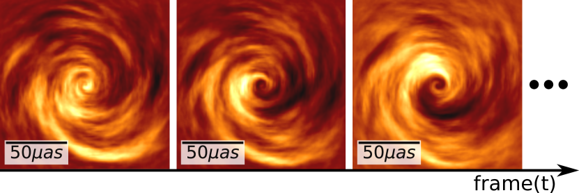
Figure 8: A sequence of three frames of statistical evolution $\exp\left\{\rho(t,x,y)\right\}$ that was sampled using inoisy. The random field was generated with correlations that mimic a disk rotating clockwise. Here the image sequence corresponds to $\sim 10$ min of observation time.

To mimic the temporal variability of Sgr A^∗, the geometric models, denoted by $I_{\rm geo}(x,y)$, are modulated by a temporal evolution sampled from a statistical model: inoisy (Lee & Gammie, 2021). This model enables sampling random spatio-temporal fields, $\rho(t,x,y)$, according to specified local correlations. Lee & Gammie (2021) and Levis et al. (2021) showed that inoisy is able to generate random fields that capture the statistical properties of accretion disks (see Figure 8). Using this model we modulate the static geometric models according to

$$I(t,x,y)=I_{\rm geo}(x,y)\exp\left\{\rho(t,x,y)\right\}.$$ (9)

Figure 7 shows both the time-average and a single snapshot of each model highlighting the effect of temporal evolution.

The inoisy model parameters were selected to generate a similar degree of time-variability as Sgr A^∗ measurements. We impose the following conditions to match metrics of temporal variations; (1) the mean of each movie’s total flux is 2.3 Jy, consistent with the ALMA light curve on April 7 (Section 2; Wielgus et al. 2022); (2) the standard deviation of the total flux is in the range of 0.09-0.28 Jy, as seen in the ALMA and SMA light curves and intra-site baselines; (3) the $\mathcal{Q}$-metric (Roelofs et al., 2017) of the intrinsic closure phase variability is comparable with Sgr A^∗ data on all triangles.

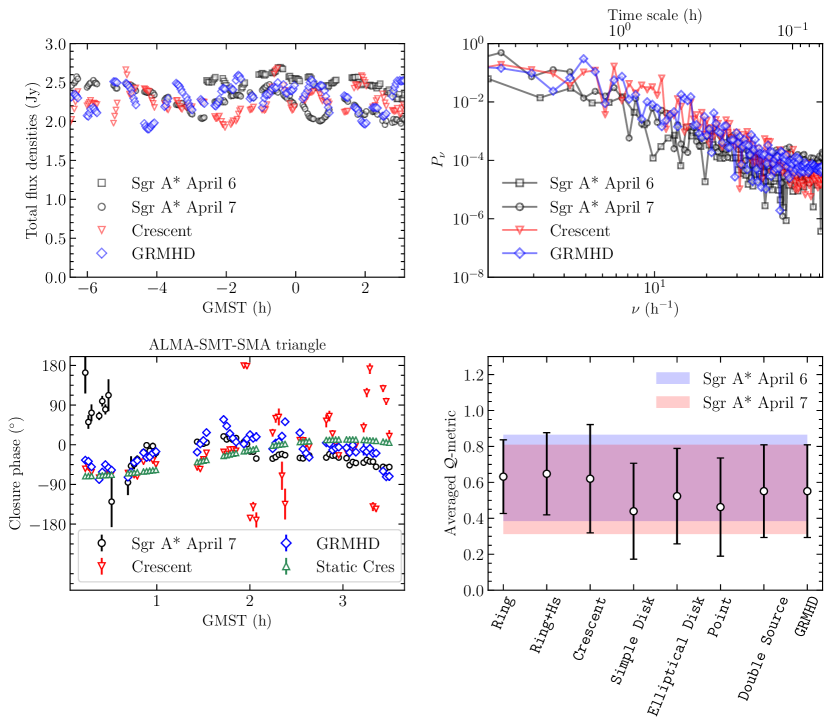
Figure 9: Temporal variability in Sgr A^∗ and synthetic data. (top left) Light curves of ALMA Sgr A^∗ data (gray points), the crescent model (red points) and the GRMHD model (blue points). (top right) Power spectrum density distributions of the light curves in the same color conventions. (bottom left) Closure phases on ALMA-SMT-SMA triangle from the April 7 Sgr A^∗ data (gray), the crescent model (red), its time-averaged static image (green), and movie of the GRMHD model (blue). (bottom right) $\mathcal{Q}$-metrics of closure phases from Sgr A^∗ and synthetic data. We show the mean and standard deviation of $\mathcal{Q}$-metrics over all independent triangles for each data set, overlaid by two shaded areas indicating the corresponding ranges for Sgr A^∗ data on April 6 and 7.

Figure 9 shows temporal variations in the total flux density and closure phases with comparison to Sgr A^∗ data. The synthetic data variability is able to capture the real data light curve variablity. Moreover, the power spectrum density distributions of the light curves from synthetic models are broadly consistent with Sgr A^∗ data. For closure phases, inoisy produces data with visible time variability seen in high S/N triangles, such as the ALMA-SMT-LMT triangle. These synthetic movies also roughly match the Sgr A^∗ variability amplitudes, averaged over all triangles, as evaluated using the $\mathcal{Q}$-metric. We note that while these synthetic data are in good agreement of the above aspects of the EHT data, their variability amplitudes in Fourier domain are slightly less than Sgr A^∗ data (see Table 2 in Section 3.2).

5.2 GRMHD Model

In addition to the geometric models, we also generated synthetic data from GRMHD simulations to evaluate the performance of our imaging procedures on more complicated physically-motivated models of Sgr A^∗. These GRMHD models are selected from the simulation library presented in Paper V, and are in general agreement with Sgr A^∗ data (Paper V section 3.1.2). Section 6.4.2 shows the result of applying our imaging procedure to a weakly magnetized “standard and normal evolution” (SANE) model, with dimensionless spin $a_{*}=-0.94$, electron temperature ratio $R_{\mathrm{high}}=160$, and viewing inclination $i=50^{\circ}$. Although failed in other constraints (see Paper V appendix A), this model satisfies the same criteria used for selection of the geometric models as seen by the resulting visibility amplitudes (Section 5.1.1) and temporal variability (see Section 5.1.2), as shown in Figure 9. Figure 7 shows a single snapshot frame of the GRMHD movie along with a time-averaged structure. The GRMHD movie frames contain a sharp photon ring with a faint emission broadly extended over $\sim 100\,\mu$as. Some of the frames contain notable spiral arm features surrounding the photon ring and extending beyond the compact structure (refer to the SANE frames shown in Figure 25). This spiral arm feature is smoothed out by averaging over the observational time.

In addition, Appendix H shows the result of applying the same imaging procedure on a strongly magnetized “magnetically arrested disk” (MADs) model with positive spin, which passes more observational constraints and is in the “best bet region” considered by Paper V. By using these two GRMHD models, generated with different physical parameters, we demonstrate that our imaging procedure and the resulting performance is robust against the details of GRMHD models.

6 Imaging Surveys with Synthetic Data

We conducted surveys over a wide range of imaging assumptions with four scripted imaging pipelines using RML, CLEAN and a Bayesian posterior sampling method. The surveys were performed on the synthetic data sets presented in Section 5 as well as on the real Sgr A^∗ data. Reconstructing synthetic data with exactly the same procedure used on Sgr A^∗ allows us to assess our ability to identify the true underlying time-averaged morphology. Both synthetic and real Sgr A^∗ data sets were pre-processed with a common pipeline described in Section 6.1. We describe the RML and CLEAN imaging parameter surveys in Section 6.2 and imaging with a Bayesian posterior sampling method in Section 6.3. Images of synthetic data from imaging surveys are described in Section 6.4. We present images of the actual Sgr A^∗ data in Section 7.

6.1 Common Pre-imaging Processing

To reconstruct a time-averaged image of Sgr A^∗, each pipeline used the original calibrated data sets described in Section 2 and/or data sets further normalized by the time-dependent total flux density of Sgr A^∗. Within each imaging pipeline, data sets were first time-averaged to enhance the S/N of visibilities; each pipeline adopted a single integration time or explored multiple choices of the integration time (see Tables 3-5). After time averaging, fractional errors of 0%, 2 % or 5 % were added to the visibility error budget in quadrature to account for the non-closing systematic errors (refer to Paper II).

As described in Sections 3.1 and 3.2, we employ additional strategies to mitigate extrinsic scattering and intra-day variations. To assess these proposed strategies, and our ability to account for these two effects in the imaging process, we incorporate parameterized error budgets and systematically explore the various assumptions on these two effects in the RML and CLEAN surveys discussed in Section 6.2. In total, we potentially include up to three additional noise budgets that account for 1) systematic error, 2) interstellar scattering, and 3) time variability.

The second budget accounts for the substructure arising from refractive scattering. We added the anticipated refractive noise level for the observed (i.e. interstellar-scattered) visibilities using two base models described in Section 3.1. The first model we explore is the Const model, which adds a constant noise budget across all visibilities prior to deblurring; we examined two noise levels: 0.4 % and 0.9 % of the total flux density at each time segment (i.e., Const and 2$\times$Const). The second model explored is the J18model1 (J18) model, which is no longer constant in the $(u,v)$-space; we adopt two scaling factors of 1.0 and 2.0 for this noise floor (i.e, J18model1 (J18) and 2$\times$J18model1 (2$\times$J18). The two noise levels adopted in each model reasonably cover differences in the noise levels caused by different potential intrinsic structures (see Section 3.1). After including one of the above budgets for the refractive noise, visibilities were divided by the diffractive scattering kernel based on the J18 model to mitigate diffractive scattering. In addition to the above four sets of the scattering mitigation schemes, we attempted imaging without any form of scattering mitigation to probe the interstellar-scattered source structure of Sgr A^∗ (referred to as on-sky images).

The third noise budget explored accounts for the structural deviations from the time-averaged morphology due to the intra-day variations. We further inflated the visibility error budget using the variability noise model described by Equation 2 in Section 3.2. This budget was added in quadrature to the visibility noise budget, after being normalized by the time-dependent total flux density. We systematically explored various sets of parameters in Equation 2 including the variability rms level at 4 G$\lambda$ ($a$), the break location ($u_{0}$), and the variability power-law spectra index at long baselines ($b$). Similar to scattering, we also attempted reconstructions without this error budget (i.e., assuming no intra-day variation in data).

6.2 RML and CLEAN Imaging Parameter Surveys

In a manner similar to previous EHT imaging of M87^∗ (; ), we explore how recovered images are influenced by different imaging and optimization choices. In particular, we objectively evaluate each set of imaging parameters in scripted RML and CLEAN imaging pipelines using synthetic data with known ground truth images. Each parameter survey leads to a Top Set of parameters: parameter combinations that each produce acceptable images on our entire suite of synthetic data. The distribution of Sgr A^∗ images recovered with the Top Set parameter combinations reflects our uncertainty due to modeling and optimization choices made in imaging; thus, it is different from a Bayesian posterior and instead attempts to characterize what is sometimes referred to as epistemic uncertainty.

Table 3: Parameters in the DIFMAP Pipeline Top Set

April 7 (8400 Param. Combinations; 1626 in Top Set)
Systematic	0		0.02		0.05
error	25.6%		36.8%		37.5%
$\bf Ref\ Type$	No	Const	2$\times$Const		J18	2$\times$J18
	14.9%	20.7%	21.3%		22.1%	20.9%
$\bf a_{\bf\rm psd}$	No	0.015		0.02		0.025
	5.1%	28.5%		32.1%		34.3%
$\bf b_{\bf\rm psd}$	No	1		3		5
	5.1%	20.2%		35.5%		39.2%
$|u|_{0}$	No			2
	5.1%			94.9%
Time average	10			60
(sec)	45.0%			55.0%
ALMA weight	0.1			0.5
	41.1%			58.9%
UV weight	0			2
	54.7%			45.3%
Mask Diameter	80	85	90	95	100	105	110
($\mathrm{\mu as}$)	0.2%	2.5%	22.3%	25.0%	21.3%	20.0%	8.7%

Note. In each row, the upper line with bold text shows the surveyed parameter value corresponding to the parameter of left column, while the lower line shows the number fraction of each value in Top Set. The total number of surveyed parameter combinations and Top Set are shown in the first row.

Table 4: Parameters in the eht-imaging Pipeline Top Set

April 7 (112320 Param. Combinations; 5594 in Top Set)
Systematic	0		0.02	0.05
error	21.4%		36.7%	41.8%
$\bf Ref\ Type$	No	Const	2$\times$Const	J18	2$\times$J18
	27.0%	23.9%	20.6%	16.4%	12.1%
$\bf a_{\bf\rm psd}$	No	0.015		0.02	0.025
	11.4%	40.6%		26.6%	21.4%
$\bf b_{\bf\rm psd}$	No	1	2	3	5
	11.4%	24.8%	20.4%	21.5%	21.8%
$|u|_{0}$	No			2
	11.4%			88.6%
TV	$\bf 0$	0.01		0.1	1
	13.2%	16.0%		36.1%	34.7%
TSV	$\bf 0$	0.01		0.1	1
	29.5%	32.3%		26.6%	11.5%
Prior size	70		80	90
($\mathrm{\mu as}$)	33.9%		34.7%	31.4%
MEM	$\bf 0$	0.01		0.1	1
	7.8%	18.4%		54.3%	19.6%
Amplitude	0		0.1	1
weight	0.9%		23.3%	75.8%

Note. Same as Table 3

Table 5: Parameters in the SMILI Pipeline Top Set

April 7 (54000 Param. Combinations; 2763 in Top Set)
Systematic	0		0.02	0.05
error	33.9%		33.3%	32.8%
$\bf Ref\ Type$	No	Const	2$\times$Const	J18	2$\times$J18
	15.7%	22.1%	18.5%	21.4%	22.3%
$\bf a_{\bf\rm psd}$	No	0.015		0.02	0.025
	7.5%	37.2%		26.7%	28.6%
$\bf b_{\bf\rm psd}$	No	1	2	3	5
	7.5%	16.8%	27.7%	31.9%	16.1%
$|u|_{0}$	No		1	2
	7.5%		40.7%	51.8%
TV	$\bf 10^{2}$	$\bf 10^{3}$		$\bf 10^{4}$	$\bf 10^{5}$
	8.6%	46.7%		44.4%	0.3%
TSV	$\bf 10^{2}$	$\bf 10^{3}$		$\bf 10^{4}$	$\bf 10^{5}$
	38.7%	53.3%		8.0%	0.0%
Prior size	140		160	180
($\mathrm{\mu as}$)	33.0%		33.6%	33.3%
$\bf\ell_{1}$	0.1		1	$\bf 10$
	44.8%		54.8%	0.3%

Note. Same as Table 3

6.2.1 Imaging Pipelines

Similar to previous EHT work (; ), we designed three scripted imaging pipelines utilizing the DIFMAP, eht-imaging and SMILI software packages. After completing the common pre-imaging processing of data (Section 6.1), each pipeline reconstructs images using a broad parameter space (e.g., weights for the regularization functions, mask sizes, station gain constraints, variability noise budget parameters, etc.). We describe each pipeline in detail in Section D.1, Section D.2, and Section D.3.

Each pipeline explored on the order of $10^{3-5}$ parameter combinations, as summarised in Table 3, 4, and 5 for DIFMAP, eht-imaging, and SMILI, respectively. Each pipeline has some unique choices that are fixed (e.g. the pixel size, or the convergence criterion) and surveyed (e.g., the regularizer weights), while some parameters are commonly explored (e.g. parameters for the scattering and intra-day variations in Section 6.1).

While all imaging pipelines adopt the common pre-processing of data described in Section 6.1, there are some differences in data processing. For instance, the noise budgets for refractive scattering and intra-day variability are updated during self-calibration rounds in SMILI. RML imaging pipelines (eht-imaging and SMILI) adopt the same prior and initial images across all synthetic and real data sets. The DIFMAP pipeline uniformly explores a library of initial models for a first phase self-calibration, selecting the one that provides the best fit to the closure phases after a first run of cleaning (see Section D.1). All three pipelines use combined low- and high-band data for imaging without any data flagging (including the intra-site baselines).

6.2.2 Top Sets of Imaging Parameters via Surveys on Synthetic Data

Large imaging surveys on synthetic data facilitate the evaluation of different potential parameter combinations. Following M87^∗ Paper IV, the principal output from each parameter survey is a Top Set: a set of parameter combinations that produce acceptable images on the suite of synthetic data presented in Section 5.

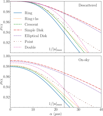
Figure 10: Normalized cross correlation, $\rho_{\rm NX}$, between time-averaged ground truth images and their corresponding blurred images, as a function of the blurring kernel size. These curves are shown for both the intrinsic images (top panels) and the scattered (i.e., on-sky) images (bottom panels). The dashed black line indicates the angular resolution equivalent to the maximum fringe spacing of Sgr A^∗ observations, 24 $\mathrm{\mu as}$; the corresponding value of $\rho_{\rm NX}$ at 24 $\mathrm{\mu as}$ is used to define a threshold that selects which DIFMAP, eht-imaging and SMILI imaging parameter combination are applied to Sgr A^∗ data.

The fidelity of synthetic image reproduction is measured using the normalized cross-correlation between the reconstructed images and ground truth images. We define the normalized cross-correlation of two images $X$ and $Y$ made of $N$ pixels as

$$\rho_{\rm NX}=\frac{1}{N}\sum_{i}\frac{(X_{i}-\braket{X})(Y_{i}-\braket{Y})}{\sigma_{X}\sigma_{Y}}.$$ (10)

Here $X_{i}$ and $Y_{i}$ denote the image intensity at $i$-th pixel, $\braket{X}$ and $\braket{Y}$ denote the mean pixel values of the images, and $\sigma_{X}$ and $\sigma_{Y}$ are the standard deviations of pixel values. The position offset between the frames is corrected by shifting one frame relative to the other along R.A. and decl. and identifying the shift coordinate that corresponds with the largest $\rho_{\rm NX}$.

In order to recover a Top Set, a threshold for $\rho_{\rm NX}$ is defined for each synthetic data set. Imaging parameter combinations that recover images that score above that thresholds for all synthetic data set are selected as Top Sets. The threshold values of $\rho_{\rm NX}$ are determined in a manner similar to M87^∗ Paper IV. For each “ground truth" image (obtained by time averaging the synthetic movie), we evaluate $\rho_{\rm NX}$ between the ground truth image and the same image blurred with a Gaussian beam of FWHM equivalent to the maximum fringe spacing of the Sgr A^∗ observations, 24 $\mathrm{\mu as}$. This value of $\rho_{\rm NX}$ quantifies the potential loss of the image fidelity due to the limited angular resolution. Figure 10 shows examples of the $\rho_{\rm NX}$ curves between unblurred and blurred ground truth images as a function of the blurring size; the critical value corresponds to those at $\alpha=24$ $\mathrm{\mu as}$. Note that this value depends on the true source structure. Unlike in M87^∗ Paper IV, we find that a relaxation of the $\rho_{\rm NX}$ threshold is required to account for the fact that we reconstruct static images from time variable data sets. Hence the critical $\rho_{\rm NX}$ values for all training data sets are multiplied by the relaxation factor of 0.95. In other words, the threshold for each synthetic data set is set to $0.95\times\rho_{\rm NX}$ for $\rho_{\rm NX}$ evaluated at $\alpha=24\mathrm{\mu as}$. This relaxed threshold allows for a large enough number of Top Set parameters to be identified for all epochs and imaging pipelines. We ensure that the relaxed threshold still reconstructs all representative ground truth morphologies; in Appendix E, the worst $\rho_{\rm NX}$ images are shown for Top Set reconstructions of each model with each imaging pipeline to demonstrate that the representative features are recovered even in the worst-fidelity Top Set images.

In Tables 3, 4 and 5, we summarize the parameters and surveyed values in each pipeline’s survey. These tables indicate the fraction of images corresponding to that parameter in each pipeline’s Top Set for April 7 data. The results on April 6 data are summarized in Appendix E. The tables also provide the total number of surveyed parameter combinations as well as the number of combinations selected for each Top Set. As seen in each table, there are more than 1000 parameter combinations in each pipeline’s Top Set for April 7, which we find is sizable enough for downstream analysis. In contrast, we find that the April 6 Top Set sizes are much smaller, likely due to the poorer $(u,v)$-coverage.

6.3 Image Posteriors with Themis

Table 6: Bayesian Imaging Priors

Parameter	Units	Prior
Control points	Jy $\mu{\rm as}^{-2}$	$\mathcal{L}(10^{-3},0.1)$
FoVx	$\mu{\rm as}$	$\mathcal{U}(50,500)$
FoVy	$\mu{\rm as}$	$\mathcal{U}(50,500)$
Raster rotation	rad	$\mathcal{U}(-0.25\pi,0.25\pi)$
Shift in $x$	$\mu{\rm as}$	$\mathcal{U}(-100,100)$
Shift in $y$	$\mu{\rm as}$	$\mathcal{U}(-100,100)$
$\ln(\sigma_{\rm ref})$	–	$\mathcal{N}(-5.5,1.0)$
$\ln(f)$	–	$\mathcal{N}(-4.6,1.0)$
$a$	–	$\mathcal{L}(a_{25\%},a_{75\%})$
$u_{0}$	–	$\mathcal{L}(u_{0,25\%},u_{0,75\%})$
$b$	–	$\mathcal{L}(b_{25\%},b_{75\%})$
$c$	–	$\mathcal{L}(1.5,2.5)$

The Bayesian imaging method employed in Themis differs from those described above in a number of respects. Most significantly, apart from sampler tuning – which affects only the efficiency with which the posterior is explored – the splined raster model has only two free parameters. Image resolution, raster orientation, the brightness at each control point, and noise model parameters are determined self-consistently by the fitting process (see Appendix A). This is achieved by replacing the hyperparameters associated with field of view, scattering threshold in the Const prescription, systematic error budget, and those that define the variability mitigation noise with fit parameters, precluding the need to survey over them. Priors for each quantity are listed in Table 6, and make use of the pre-imaging constraints described in Section 3 and listed explicitly in Table 2.

Importantly, eliminating the hyperparameters associated with the additional contributions to the visibility uncertainties eliminates the noise-related data preparation steps described in Section 6.1; we do not add any additional uncertainty prior to the Themis analysis. However, to reduce the data volume (and thus computational expense of the posterior sampling) we incoherently average the flux-normalized data over scans. To prevent significant coherence losses, prior to averaging we calibrate the phase gains of the JCMT using the intra-site baseline, JCMT-SMA, and assume that the source is unresolved at the corresponding spatial scales probed by that baseline.

The remaining two unspecified hyperparameters are the raster dimensions, $N_{x}$ and $N_{y}$. Initial guesses for these are provided by the diffraction limit; for a typical source size of $80~{}\mu{\rm as}$, $N_{x}=N_{y}=5$ is sufficient to marginally super-resolve the source. This may then be refined via a modest survey over potential values, with the final values selected by maximizing the Bayesian evidence, computed in Themis via thermodynamic integration (Lartillot & Philippe, 2006). In practice, due to the expense of such a survey, we restrict ourselves to $N_{x}=N_{y}=5$ for the validation with synthetic data sets with a sole exception. We performed a raster dimension survey for the GRMHD data set presented in Section 6.4.2, finding that $N_{x}=N_{y}=6$ is preferred.

For application to Sgr A^∗, we perform raster dimension surveys independently for April 6 and 7 as described in Section D.4, finding preferred dimensions of $N_{x}=N_{y}=6$ and $N_{x}=N_{y}=7$, respectively.

6.4 Synthetic Data Images

We first present Top Set and posterior images recovered from geometric model datasets in Section 6.4.1, followed by images recovered from the GRMHD dataset in Section 6.4.2.

6.4.1 Geometric Model Images

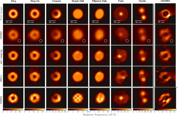
(a) Descattered Reconstructions

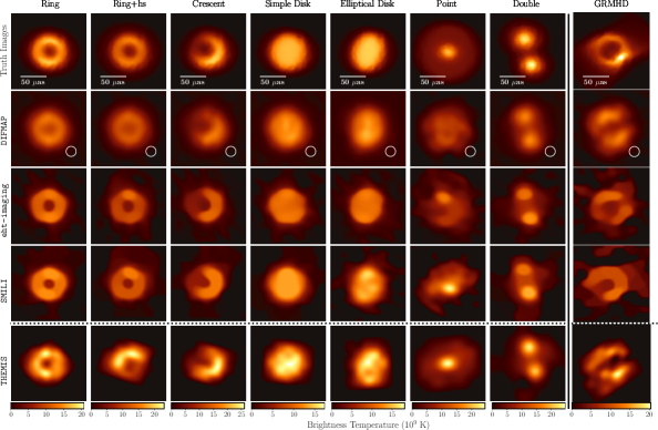
(b) On-sky Reconstructions

Figure 11: Reconstructed images of synthetic data sets on April 7 (a) with and (b) without scattering mitigation for seven geometric models and the GRMHD model. Reconstructions of each geometric model by DIFMAP, eht-imaging and SMILI pipelines are made using a parameter combination identified via cross-validation: the imaging parameters that result in the the best average $\rho_{\rm NX}$ across all other geometric models. These cross-validation results demonstrate the ability of the selected parameters to correctly reproduce novel source morphologies. GRMHD reconstructions for DIFMAP, eht-imaging, and SMILI are produced from an imaging parameter combination that performs best on all geometric models. In contrast, for Themis reconstructions the average posterior image is shown for each model; the average posterior image appears to correctly identify the true source morphology in all synthetic data sets tested.

In Figure 11, we show the time-averaged ground truth images and corresponding image reconstructions for each of the synthetic data sets with April 7 $(u,v)$-coverage. Images from all pipelines are obtained with and without scattering mitigation (henceforth, descattered and on-sky reconstructions). These descattered and on-sky reconstructions are compared to the time-averaged ground truth images of the intrinsic and scattered structure, respectively.

DIFMAP, eht-imaging and SMILI images for each geometric model in Figure 11 are obtained using cross-validation: the parameter combination that provides the best mean $\rho_{\rm NX}$ across other geometric models (i.e., except for the model being tested) are selected. The cross-validation images in Figure 11 (which are contained in each pipeline’s Top Set) successfully recover the representative morphology of each geometric model, demonstrating the capability of a single imaging parameter combination to identify various source structures. The manifestation of structure significantly different from the ground truth morphology is only seen in a small fraction of the cross-validated Top Set parameters. For instance, using the ring classification method described in Appendix F, only 2%, $<$1%, and $<$1% of the cross-validated Top Set reconstructions for the Ring model are identified as not having a ring feature for DIFMAP, eht-imaging and SMILI, respectively; the reconstruction of a non-ring morphology is also found to be limited to small fraction of 3%, 5%, and 1% for the Crescent model. Similarly, only a small fraction of the reconstructions from non-ring models are reconstructed with a ring morphology — in particular, for the DIFMAP, eht-imaging, and SMILI pipelines, 7%, 11%, and 3% and $<$1%, $<$1%, and $<$1% of the cross-validated Top Sets reconstructed a ring feature from the Point and Double source models, respectively.

For Themis reconstructions, the mean posterior image is shown for each model. Figure 11 shows that the posterior images from Themis reconstructions identify the general morphology of each geometric model. Most of Themis posterior images satisfy the criteria based on a minimum threshold of $\rho_{\rm NX}$ used in Top Set selections for DIFMAP, eht-imaging and SMILI pipelines (see Section 6.2.2), with the exception of a few models discussed below. For April 7 images, all posterior images show higher $\rho_{\rm NX}$ than the threshold except for 1% and 7% of descattered reconstructions for Double source and Ring+hs models, respectfully. For April 6, the images below the threshold are limited to 1% and 22% of descattered reconstructions for the Point and Double source models, respectively. However, 95% of on-sky reconstructions of Point source model are above the $\rho_{\rm NX}$ threshold on April 6 for Themis. The high fractions of images beyond the $\rho_{\rm NX}$ threshold for all models on April 7 demonstrate the capability of Themis pipeline to recover various representative morphologies at an acceptable fidelity.

Figure 11 also shows the resiliency of the reconstructed morphology to the scattering prescriptions. While the on-sky reconstructions without scattering mitigation tend to be slightly more blurry than those with descattering, there are not many other notable differences in their appearance. In particular, the refractive substructure, which adds spatial distortion of images on scales finer than the angular resolution of the EHT, is not well constrained in our EHT data and therefore does not strongly appear in any reconstructions. We further discuss the effects of scattering prescriptions for Sgr A^∗ images in Section 7.5.2.

6.4.2 GRMHD Reconstructions

Figure 12: The distribution of images obtained from synthetic data provided using a GRMHD movie with April 7 $(u,v)$-coverage. From left to right (separated by vertical lines), we show the distributions of Top Set images from the DIFMAP, eht-imaging and SMILI pipelines and posterior samples from the Themis pipeline; each vertical panel is further subdivided into clusters identifying common morphologies recovered by each pipeline. The figure is comprised of three horizontal panels separated by horizontal lines. The top panel shows individual images randomly sampled from different clusters. The middle and bottom panels visualize the distributions of reconstructed descattered and on-sky images for each cluster, respectively. In each panel, from top to bottom, we show the average of each cluster, the distributions of the radial profiles, and the distributions of azimuthal intensity profiles. In the radial profiles, each horizontal slice corresponds to the azimuthally-averaged intensity profile of an image, normalized by its peak value. Similarly, the azimuthal profiles show the azimuthal distribution of the radial peak intensity within a radius of 10 to 40 $\mathrm{\mu as}$, also normalized by its peak value. The dotted lines in the profiles indicate the peak radius or position angle of the ground truth GRMHD movie. The vertical order of images in both profiles is independently sorted by the peak radius or position angles; therefore the images are ordered differently in each profile distribution image. These results on synthetic data show that the Top Set and posterior samples from the imaging pipelines are able to recover ring images that resemble the true time-averaged structure of a GRMHD movie (see Figure 7). However, the imaging methods sometimes produce non-ring images that still fit the data well.

We show example GRMHD reconstructions on April 7 in the rightmost panels in Figure 11. This GRMHD simulation contains a ring with a diameter of $\sim 51$ $\mathrm{\mu as}$. GRMHD images from DIFMAP, eht-imaging, and SMILI pipelines are reconstructed with the Top Set parameter combinations that corresponds with the largest average $\rho_{\rm NX}$ value across all seven geometric models. For Themis reconstructions, on the other hand, the expected (i.e., mean) posterior image is shown.

Unlike with the simple geometric synthetic data sets, the distribution of GRMHD reconstructions show wide variations in the image appearance. Although GRMHD reconstructions in Figure 11 commonly show a ring-like morphology with a diameter of $\sim 50$ $\mathrm{\mu as}$, the azimuthal intensity distribution is not consistent across the Top Sets. In the top panels of Figure 12, we show images from GRMHD April 7 data from each pipeline, which are randomly selected from DIFMAP, eht-imaging and SMILI Top Sets and posterior images from Themis. Most of the images have clear asymmetric ring features, but a few images show non-ring structures. The diameters of ring features are broadly consistent across different reconstructions, comparable to the ground truth image. On the other hand, the azimuthal distributions are not uniquely constrained by the Top Set images — different position angles are seen in the randomly sampled images from each Top Set.

To visualize the distribution of images with different morphology, we categorize all images into three major groups: ring images peaked at PAs within (a) the range of $-180^{\circ}\leq{\rm PA}<0^{\circ}$ where the ground truth value of $-124^{\circ}$ is located, (b) the range of $0^{\circ}\leq{\rm PA}<180^{\circ}$, and (c) the remaining images comprising non-ring or other ring-like images with much less consistency. The definition of a ring used in this paper to classify ring versus non-ring images is described in Appendix F. Note that the particular definition of a ring will influence the quoted percentages of ring and non-ring images recovered. We find that the particular definition chosen in this paper results in classification that largely aligns with human perception. However, the classification of images that are borderline between ring and non-ring classification are sensitive to the exact criteria used. Therefore ring definitions that make use of different criteria can lead to classification that still largely aligns with human perception but varies somewhat in the ring classification percentages quoted in this paper.

In the middle and bottom panels of Figure 12, we summarize the distribution of images from each pipeline with and without scattering mitigation, respectively. The GRMHD images within each pipeline’s Top Set are clustered into image modes. The upper sub-panel shows the mean image of each cluster, indicating a common or representative morphology recovered. The middle sub-panel shows the distributions of the azimuthally-averaged radial intensity profiles, where the vertical order of images is sorted by the peak radii of the profiles. The lower sub-panel shows the azimuthal distribution of the radial peak intensity within a radius of 10 to 40 $\mathrm{\mu as}$.

Figure 12 demonstrates that most of the Top Set or posterior images reconstruct ring images from the GRMHD data set. In particular, the radial profiles of the first two ring modes show a broad consistency of the peak radius around $\sim$25 $\mathrm{\mu as}$ which implies a diameter of $\sim$50 $\mathrm{\mu as}$ consistent with that of $\sim$50 $\mathrm{\mu as}$ for the ground truth model. The capability of identifying a ring with the consistent diameter does not appear to depend on the scattering mitigation. Similarly to geometric synthetic data (see Section 6.4.1), the scattering mitigation does not significantly affect the resulting source morphology in the reconstructed images, except that the images without scattering mitigation tend to be slightly broader. Refractive substructure does not appear in the reconstructed on-sky images, again indicating that the appearance of the refractive substructure is not strongly constrained with EHT 2017 data.

As seen in the azimuthal profiles, each pipeline provides at least one asymmetric ring mode with the peak position angle roughly consistent with that of the mean ground truth image of $-124^{\circ}$. For this particular GRMHD example, this mode is found to be the most popular mode in most pipelines. However, Figure 12 indicates that the ring mode with the correct orientation is not always identified as the most popular mode among image samples — for instance, the correct orientation is not identified as the most popular ring mode for the eht-imaging on-sky pipeline. Therefore, caution should be taken, as the popularity of a mode in an RML or CLEAN pipeline’s Top Set does not necessarily always correspond with the true underlying structure.

We find that key takeaways from the GRMHD example are consistent with the “best-bet” GRMHD models presented in Paper V, identified based on various criteria using both EHT and non-EHT data. In Appendix H, we show example reconstructions of a “best-bet” GRMHD model. We find the identification of a ring morphology for the vast majority of the Top Set reconstructions, however multiple ring modes and non-ring images are still reconstructed. Note also that the peak position angle of the ground truth “best-bet” GRMHD model is not necessarily identified as the most popular mode reconstructed in each Top Set. These results indicate that the same trends are seen across multiple GRMHD models that are broadly consistent with EHT data.

7 Horizon-scale Images of Sgr A^∗

Figure 13: In the top main panel we show the representative image of Sgr A^∗ obtained with the EHT from observations on 2017 April 7. This top image is obtained by averaging the bottom four images. On the bottom from left to right, we show the average images of three prominent ring clusters with different azimuthal structures and a non-ring cluster. The height of the colored bar (bottom left in each panel) represents the relative fraction of images in the Top Sets for each cluster. We note that Themis posterior sample only includes ring images. In each cluster, the image is computed through a weighted average over the descattered reconstructions, including all Top Set images from the three imaging methods (DIFMAP, eht-imaging, and SMILI) and 1024 images randomly selected from descattered posteriors from Themis. Images are weighted by the inverse of the total number of Top Set or posterior images used from each pipeline, so that pipelines are represented equally in each image. Note that DIFMAP model images are convolved with 20 $\mathrm{\mu as}$ beam (represented by the inset circle), while no blurring is applied to the rest of images.

Having determined Top Set imaging parameters for RML and CLEAN, and validated posterior estimation for Themis via tests on synthetic data (Section 6), we now show the result of these methods applied to Sgr A^∗ data from the 2017 EHT observations. Unlike in the previous EHT imaging of M87^∗ (; ), Sgr A^∗’s recovered structure depends somewhat on the imaging strategy and parameter choices. Thus, this section presents our main imaging results and analyzes how the image structure is affected by different imaging choices.

We begin in Section 7.1 by giving an overview of the results, followed by a more detailed discussion of the image structures recovered in each pipeline’s Top Set or posterior in Section 7.2. Average images across pipelines, calibrated data sets, and observing days are discussed in Section 7.3. In Section 7.4 we present Sgr A^∗ imaging obtained by combining the data sets for April 6 and 7. In Section 7.5 we address the question of whether Sgr A^∗ is a ring, and explore how the recovered images are affected by the scattering and temporal variation mitigation strategy.

7.1 Overview of Recovered Sgr A^∗ Structure

Figure 13 summarizes the common morphologies recovered from Sgr A^∗ data by the four imaging pipelines for April 7. We find that the vast majority are rings that can be classified into three different clusters with varying azimuthal structures (Section 7.2), shown in the three bottom left panels of Figure 13, and a small fraction of non-ring images that also fit the Sgr A^∗ data well (bottom right panel in Figure 13). Since these non-ring images are not as consistent in structure they largely blur out when averaged together and primarily emphasize a double-structure that is sometimes present. The representative Sgr A^∗ image obtained by averaging reconstructions from all four clusters is shown in the large top panel of Figure 13, corresponding to that of a ring with a diameter of $\sim$50 $\mu$as (Section 8).

Figure 14: The distribution of reconstructed Sgr A^∗ images on April 7. We show the distribution of images from each pipeline for each cluster with the same convention as Figure 12. From left to right (separated by vertical lines), we show the distributions of Top Set images from the DIFMAP, eht-imaging, and SMILI pipelines and posterior samples from the Themis pipeline; each vertical panel is further subdivided into clusters identifying common morphologies recovered by each pipeline. The figure is comprised of three horizontal panels separated by horizontal lines. The top panel shows individual images randomly sampled from different clusters. The middle and bottom panels visualize the distributions of reconstructed descattered and on-sky Sgr A^∗ images for each cluster, respectively. In each panel, from top to bottom, we show the average of each cluster, the distributions of the radial profiles, and the distributions of azimuthal intensity profiles. Note that Themis images have only three clusters for each of descattered and on-sky reconstructions — their descattered posterior does not contain a non-ring cluster and their on-sky posteriors do not contain an east PA ring cluster.

Figure 15: Comparison of image characteristics between each cluster. The radial and azimuthal values are the fractional central brightness and azimuthal peak brightness PA, respectively. The left panel shows the distribution of all Top Set and posterior images with all imaging pipelines (DIFMAP, eht-imaging, SMILI, and Themis) and scattering mitigation (descattered and on-sky), including the three ring clusters with different peak azimuthal brightness [red ($-180^{\circ}\leq{\rm PA}<-70^{\circ}$), blue ($-70^{\circ}\leq{\rm PA}<40^{\circ}$), and green ($40^{\circ}\leq{\rm PA}<180^{\circ}$)], and a non-ring cluster (white). The right eight panels show distributions within a single imaging pipeline and scattering mitigation. The majority of azimuthal peak brightness among each ring cluster is shown in the outer gray histogram in each panel.

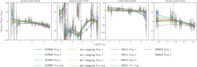
Figure 16: Closure phases plotted as function of GMST on four selected triangles from April 7 observations. Each line indicates the corresponding closure phase curves from a single Top Set and posterior image randomly selected from each cluster. The error bars of Sgr A^∗ data include the fractional 1 % noise budget for systematic error and a representative budget for scattering and temporal variability – in particular, the J18model1 refractive noise model and a variability model with parameters $a=0.02$, $u_{0}=2$, $b=2.5$, and $c=2$. These additional noise budgets are all added to the 60 second complex visibility noise budget prior to forming closure quantities. All images show reasonable fits to Sgr A^∗ data as they all are within two standard deviations of the observed data.

7.2 Clustering of Recovered Sgr A^∗ Images

To effectively visualize the distributions of Sgr A^∗ images, we cluster all reconstructed Top Set and posterior images using a similar criteria to that used in Section 6.4.2 and Figure 12 (see Appendix F for details). Images with a ring feature are grouped by the peak PAs in the southwest ($-180^{\circ}\leq{\rm PA}<-70^{\circ}$), northwest ($-70^{\circ}\leq{\rm PA}<40^{\circ}$), and east ($40^{\circ}\leq{\rm PA}<180^{\circ}$) directions. The Sgr A^∗ image clustering results for each pipeline are summarized in Figure 14; here, we focus on the observed date of April 7 with the HOPS data reduction pipeline (see Section 7.3 for April 6 and CASA-based reconstructions). The results of the DIFMAP, eht-imaging, SMILI, and Themis pipelines are displayed from left to right. Images are separately clustered within each pipeline.

The middle and bottom panels of Figure 14 show each cluster’s average image for the descattered and on-sky images, respectively. To better visualize the properties of individual Sgr A^∗ images, we present three randomly selected descattered images from each cluster in the columns of Figure 14’s top panel; within each cluster images appear to have largely consistent morphologies.

The percentages in each panel of Figure 14 show the fraction of Top Set or posterior images contained in that particular cluster. These percentages indicate that most of the Top Set and posterior images have ring structures. For instance, the fraction of non-ring cluster images is $\leq 5$ % of the Top Set descattered images from DIFMAP, eht-imaging, and SMILI imaging pipelines. Although this is significant, we note that in the case of the Top Sets this does not constitute a likelihood and therefore the reported fractions should not be considered as an exact measure of our degree of certainty. In addition, only ring images appear in Themis posterior estimation of descattered images.

The bottom row of both the middle and bottom panel of Figure 14 shows the azimuthal distribution of the radial peak intensity within a radius of 10 to 40 $\mathrm{\mu as}$. These profiles are sorted within each cluster by the location of peak brightness to best accentuate variations within a cluster. By inspecting the profiles in each cluster it can be seen that three primary brightness distributions, with a peak brightness at $\sim-140^{\circ}$, $-40^{\circ}$, or $70^{\circ}$, appear across the pipelines. Thus, even when we restrict our attention to ring-like morphology reconstructions, it is difficult to constrain the azimuthal profile around the ring via imaging. This azimuthal uncertainty could be due to data properties (e.g., sparsity or low S/N data) or variation in the intrinsic azimuthal structure of Sgr A^∗ due to intra-day evolution.

To visualize the image-domain differences among each cluster, we compare in Figure 15 the relationship between the fractional central brightness ($f_{c}$, radial values) and the azimuthal peak brightness (${\rm PA}$, azimuthal values). The polar distribution of Top Sets and posterior images among all imaging pipelines and with and without scattering mitigation (left panel in Figure 15) shows that most of the ring images within each different cluster (indicated by the red, blue, and green points) have a smaller fractional central brightness ($f_{c}\lesssim 0.5$) than that for the images in the non-ring cluster ($f_{c}\gtrsim 0.5$).

The histogram of the azimuthal peak brightness distributions shown in left panel in Figure 15 provides a clear visualization of the clustering of ring images around position angles of $\sim-140^{\circ}$, $-40^{\circ}$, or $70^{\circ}$, which correspond to the locations of the three knots that commonly appear in ring images. Changes in position angle mostly reflect variations in the relative brightness of these knots. For the case of non-ring images the position angles are, as expected, more randomly distributed. Figure 15 also confirms that the fractional central brightness are systematically larger for the on-sky images due to the angular broadening produced by the interstellar scattering.

Both the ring and non-ring morphologies identified in Top Set and posterior images show reasonable fits to Sgr A^∗ data. In Appendix E, we show $\chi^{2}$ distributions of Top Set images to Sgr A^∗ data. After adding the budgets of non-closing systematic errors, representative refractive noise, and time variability, all Top Set images result in a $\chi^{2}<2$ for both closure phases and log closure amplitudes – we refer the reader to (Paper IV) and (M87^∗ Paper IV) for a discussion of these data products and $\chi^{2}$ distributions. In Figure 16 we compare closure phases of Sgr A^∗ to those of individual images from each cluster and pipeline for four selected closure triangles. As indicated by the $\chi^{2}$ metrics, multiple ring and non-ring images fit the observed closure phases within the range of deviations anticipated due to temporal variability and refractive scattering effects. Therefore, none of the identified clusters can be excluded from possible Sgr A^∗ morphologies in terms of the goodness of fit to Sgr A^∗ data (or through synthetic data tests presented in Section 6).

7.3 Average Sgr A^∗ Images across Pipelines

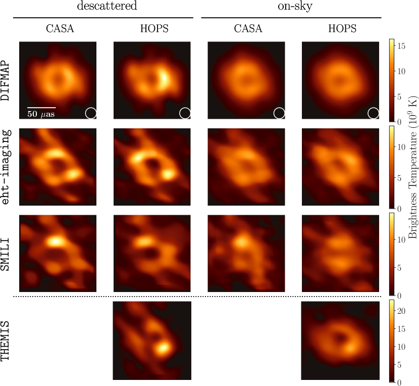
(a) April 6

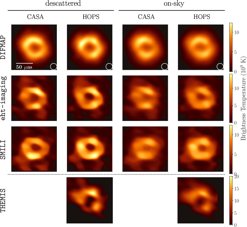
(b) April 7

Figure 17: The dominant recovered morphology in Sgr A^∗ descattered and on-sky reconstructions identified from two VLBI data products (CASA and HOPS data) with all four imaging pipelines (DIFMAP, eht-imaging, SMILI and Themis) for two observing days (April 6 and 7). Each panel shows the average image of the corresponding Top Set images for DIFMAP, eht-imaging and SMILI pipelines, and the average posterior image for Themis pipeline. Only the HOPS data has been imaged using the Themis pipeline.

Figure 17 shows the average of Sgr A^∗ images reconstructed by each of the four imaging pipelines (DIFMAP, eht-imaging, SMILI, and Themis) from each calibrated data set (CASA and HOPS) on each observing day (April 6 and 7). Only images from the HOPS data product have been reconstructed using the Themis pipeline. The images from DIFMAP, eht-imaging and SMILI are obtained by averaging their respective Top Set images; these average images show the dominant features identified across different combinations of the selected imaging parameters in the Top Sets (refer to Section 6). For the Themis reconstructions we instead show the mean of each posterior obtained by averaging all the posterior samples. Figure 17 shows that the majority of images contain a ring-like structure. This ring morphology is common among all imaging pipelines, and is resilient to the scattering mitigation strategy employed (as discussed in Section 7.5.2). Additionally, we recover largely consistent images between data calibrated by the HOPS and CASA calibration pipelines. Although we recover images with a ring morphology in the majority for all pipelines on April 7, these average images also highlight that the azimuthal brightness distribution is sensitive to small changes in the data and imaging strategy.

7.4 Imaging Combining April 6 and 7 Data Sets

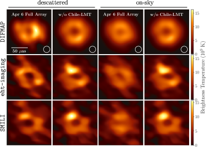
Figure 18: The effect of removing the Chile-LMT baseline from April 6 data reconstructions. Each panel shows the average image of the Top Set images for the DIFMAP, eht-imaging and SMILI pipelines from April 6 and the HOPS data product for the descattered and on-sky reconstructions. For comparison we show the average images obtained from full data sets as well as image obtained from data without the Chile-LMT baselines. This Chile-LMT baseline appears near the visibility null, and appears to exhibit significant intra-day variations on April 6 that is likely not captured by the variability noise model presented in Section 3.2.

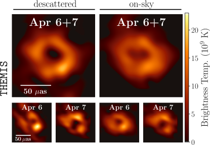
Figure 19: Mitigation of the apparent strong intra-day variations seen in April 6 through Themis imaging of the combined April 6 and 7 data. For comparison we show the average posterior images from April 6 and 7 independently and that obtained by combining the data sets for April 6 and 7, exhibiting a clear ring for the descattered and on-sky reconstructions.

In Figure 17 we show results from April 6 data, reconstructed using the same imaging procedure as April 7. We note that although a ring feature appears in most of these reconstructions, it is less prominent. The images also contain a diagonal rail-like feature going from northeast to southwest that corrupts the ring. This feature is especially prominent in the Themis April 6 descattered reconstruction. This corrupted or non-ring mode is likely emphasized in Themis imaging compared to RML and CLEAN pipelines due to the goal of Themis image samples to characterize the probability of an image rather than represent the variety of possible images that can fit the data.

Through an in-depth inspection of the April 6 data, documented in Paper IV, the Chile-LMT baselines (i.e., ALMA-LMT and APEX-LMT baselines) were identified as having large coherent visibility swings that are not effectively mitigated by the noise model on a single day, causing this particular feature to arise. Figure 18 shows the reconstructions using the DIFMAP, eht-imaging   and SMILI imaging pipelines when these particular baselines have been flagged, resulting in a cleaner ring structure.

The large visibility swings on the Chile-LMT baselines could be the cause of variability around Sgr A^∗ that exceeds expectations set by the incorporated stationary noise model presented in Section 3.2. In particular, we believe that the variability noise model should capture Sgr A^∗’s stochastic evolution in expectation, but a single night may contain non-stochastic short-lived variability that can bias a single day’s reconstruction. Correlated variability may be mitigated via multi-day fits, which combine statistically independent structural fluctuations; this better matches the assumption within our variability mitigation scheme of an underlying stochastic process, though does carry with it the additional assumption that Sgr A^∗ is statistically stationary over the multiple days combined. Therefore, in addition to the single day analyses performed by all imaging methods, the Themis image model was also fit to the combined April 6 and 7 scan-averaged data from high and low bands for the HOPS data product. The resulting static image shown in Figure 19 represents an image recovered from the combined data sets. All images within the multi-day Themis posterior exhibit a clear ring-like structure.

7.5 Is Sgr A^∗ a Ring?

Our primary imaging goal is to answer the question: “Is Sgr A^∗ a ring?”. Although our reconstructions are overwhelmingly dominated by ring images, there is a small number of non-ring images that fit the data well and cannot easily be excluded through additional tests. There are at least three possible reasons for the recovery of non-ring reconstructions of Sgr A^∗: 1) Sgr A^∗’s intrinsic structure is not ring shaped, 2) scattering causes a distortion of a ring morphology, resulting in a non-ring image, and 3) imaging algorithms recover an incorrect source structure, aggravated by challenges of sparse $(u,v)$-coverage and Sgr A^∗’s intra-day variation. In this section we will explore these three possible origins of non-ring structure. Based on this exploration we conclude that there is evidence that the non-ring reconstructions are caused by our imaging algorithms resulting from the limited $(u,v)$-coverage and rapid variability, rather than being intrinsic to Sgr A^∗.

7.5.1 Manifestation of Rings from Intrinsic Non-rings

The first possible explanation for the small percentage of non-ring reconstructions of Sgr A^∗ is simply that Sgr A^∗ does not possess a ring morphology. Although this possibility cannot be ruled out completely, we explore the possibility of a potential bias in our imaging approach towards recovering ring images from underlying non-ring sources.

There is always a possibility that the parameters initially explored by the RML and CLEAN parameter surveys were inadvertently biased to produce mostly ring images. This would result in an artificially high percentage of ring reconstructions that could give overconfidence in an incorrect ring solution. To explore this hypothesis we inspect the percentage of ring and non-ring images of Sgr A^∗ that are in the initial parameter survey versus the restricted Top Set on April 7. We find that although ring images make up a large percentage of the initial parameter surveys, 91%, 84%, 60% for DIFMAP, eht-imaging, and SMILI respectively for the descattered reconstructions, this number becomes significantly larger after Top Set selection. In particular, the percentage of ring images raises to values of 95%, 97%, 98%, respectively. Therefore, when we restrict to those parameters that can best disambiguate between the different ring and non-ring source morphologies contained in our synthetic data sets (Section 5.1), the number of ring images increases. We also note that Themis posterior samples for April 7 only contains ring images.

To further test the possibility that we are biased to recover primarily rings from underlying non-ring sources, we have explored the performance of our imaging methods on non-ring synthetic data sets to see how they compare to Sgr A^∗ results. In particular, we performed a Top Set analysis on the Point and Double source models. Two “cross-validation" Top Sets were identified by excluding the performance of either the Point or Double source model and only using the remaining six geometric models in selection of the imaging parameters. These two cross-validation Top Set parameter sets were then applied to the Point and Double synthetic data sets. Although each cross-validation Top Set does incorrectly reconstruct some ring images, each image set primarily contains reconstructions that look similar to the ground truth Point ad Double source structure. In particular for descattered reconstructions, only 9% and $<$1% percentage of the cross-validation Top Set reconstructions possess a ring morphology, compared to 97% in Sgr A^∗ reconstructions of April 7. The Themis pipeline produces no ring images in the posterior samples for both the Point and Double data sets. Thus, in the non-ring synthetic data sets we have explored we find that the number of incorrect ring reconstructions is much less than the number that we recover for Sgr A^∗. In summary, our imaging pipelines do not appear prone to artificially create a majority of ring structures in sources that do not possess an intrinsic ring morphology.

7.5.2 Scattering’s Effect on Image Reconstruction

The second possible explanation for the non-ring reconstructions of Sgr A^∗ is that interstellar scattering causes a non-ring morphology. This could take either two forms: a) Sgr A^∗’s ring morphology has been distorted to a non-ring morphology by an interstellar scattering screen, or b) our imaging algorithms have incorporated an incorrect scattering model that reconstructs a corrupted non-ring morphology.

To address the possibility that interstellar scattering is causing Sgr A^∗’s intrinsic structure to be distorted to a non-ring, we inspect differences in the descattered versus on-sky reconstructions. As outlined in Section 3.1, descattered reconstructions attempt to mitigate two primary effects of interstellar scattering — diffractive scattering that causes angular broadening and refractive scattering that introduces small-scale structure to the on-sky image. Sgr A^∗ reconstructions in Figure 14 show that on-sky images are systematically blurrier than descattered images, as expected due to deblurring that is performed before recovering a descattered image (refer to Section 3.1.1). This systematic difference between on-sky and descattered images is also seen in synthetic data reconstructions presented in Section 6.4. This angular broadening causes the central dip of a ring to be less prominent. Nonetheless, we note that the vast majority of the on-sky (i.e., without any scattering mitigation prescription) images are still rings, with percentages of 93%, 98%, 90%, and 98% for CLEAN, eht-imaging, SMILI, and Themis, respectively. We note that it is highly unlikely that a non-ring morphology was distorted into an on-sky ring morphology by interstellar scattering.

To address the possibility that our assumed model of the interstellar scattering is reconstructing a corrupted image of the descattered source, we explore the use of multiple refractive noise models to mitigate effects of refractive substructure before deblurring (Section 6.2). The contribution of the included refractive noise budget used to mitigate scattering (for descattered reconstructions) is non-negligible for long baseline data (see Section 3.1.2 and Figure 5). Nontheless, the RML and CLEAN imaging surveys show that the choice of the refractive noise model does not significantly affect the resulting distributions of image structures. Figure 20 shows the average descattered Sgr A^∗ images (clustered into the same four morphologies as is presented in Figure 13) for each refractive noise prescription explored. The comparable fractions of images in each cluster across the different descattering strategies indicates the resiliency of the recovered image structures to different refractive noise models. Another piece of evidence suggesting that the scattering prescription does not strongly affect results can be seen in the Themis results; in Themis a constant refractive noise floor is able vary in posterior sampling of descattered images. Although an essentially unlimited refractive noise component is permitted by the Themis model, the posterior estimation instead typically chooses a noise level of $<25$ mJy, only 1% of the total flux of the source.

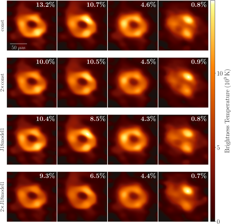
Figure 20: The range of descattered Sgr A^∗ images recovered using different refractive scattering noise models. From left to right, images are shown clustered in the same order as Figure 15. Each panel shows an average of all descattered Top Set images of Sgr A^∗ on April 7 from the DIFMAP, eht-imaging, and SMILI pipelines that were generated using the specified refractive noise model (from top to bottom: Const, 2$\times$Const, J18model1, and 2$\times$J18model1). The number on each panel shows the percentage of descattered Top Set images that were reconstructed using the specified refractive noise model. These percentages indicate that there is not a clear preference for a particular refractive noise model in Top Set selection. Additionally, the recovered image structure does not appear to correlate with the refractive noise model used.

In summary, results indicate that for EHT measurements of Sgr A^∗, interstellar scattering does not significantly affect the recovered morphology. Both on-sky and descattered images contain a majority of ring morphologies. In addition, we find the particular choice of scattering mitigation strategy only minimally affects the recovered image structures.

7.5.3 Variability’s Effect on Image Reconstruction

The third possible origin for non-ring Sgr A^∗ images is poor reconstruction quality of the imaging methods. Imaging is solving an ill-posed inverse problem due to sparse $(u,v)$-coverage, which always will have the possibility of recovering an incorrect image. This is further exasperated in imaging Sgr A^∗ by the challenges that come with recovering an evolving source. In this section we explore this possibility and find that our imaging methods often reconstruct non-ring sources for variable ring sources with a comparable small percentage as found for Sgr A^∗.

The first natural question is how our imaging methods perform on reconstructing ring sources with similar data properties as Sgr A^∗. We find that our methods produce non-ring images, even when the underlying source structure is ring-like. As an example, recall that for the variable GRMHD ring-like sources analyzed in Section 6 and Appendix H, our imaging methods produced mostly rings, but also a very small fraction of non-ring images. Therefore, we expect that for a variable ring source we would recover some non-rings that fit the data well. However, note that the number of non-rings was still fairly small in the case of the GRMHDs: 5% for the GRMHD presented in Figure 12 and 4% for the “best-bet” GRMHD presented in Figure 37. These values are comparable to the 3% of non-rings reconstructed for Sgr A^∗ descattered images across all pipelines. We also find that cross-validated Top Set images reconstructed of the Crescent and Ring geometric sources produce a small fraction of non-ring images. Note that these non-ring percentages for the GRMHD, Crescent, and Ring sources are much less than the percentage of non-rings reconstructed for the variable Point and Double source, as discussed in Section 7.5.1.

Due to Sgr A^∗’s intra-day evolution, mitigation of temporal variability in the data is important for reconstructing a single static image of Sgr A^∗. We next explore how the variability mitigation approach affects the proportion of ring versus non-ring images reconstructed. Section 3.2 introduced an approach to model the temporal variability as an additional noise budget that could be added in quadrature to the visibility thermal noise budget. The dependence of the temporal variability noise model parameters on resulting Sgr A^∗ reconstructions for the RML and CLEAN pipelines was investigated. Although a variability noise budget generally helps with imaging (as evidenced by a higher percentage of Top Set parameters selected – 89-95% of the Top Set parameter combinations include a variability noise model on April 7), similar to scattering, we find that there are no significant differences between the images recovered under different variability noise parameters. We suspect that this is partly caused by the complex interplay between regularizers and different noise model parameters (e.g., variability, scattering, and systematic), although no significant trends were identified.

In Appendix G, we demonstrate how our results are insensitive to a different method of variability mitigation. In particular, we show time-averaged morphologies identified by a large survey over full-track RML dynamical imaging parameters (refer to Section 4.4.1) that does not rely on the variability noise model presented in Section 3.2.2. We again find the ring modes to be dominantly reconstructed, while a small fraction of non-ring structures are also identified. The broad consistency indicates that our results are resilient to at least two different methods to recover time-averaged morphology.

In summary, we find that our imaging methods do reconstruct a small percentage of non-ring images from ring sources with comparable variability as that seen in Sgr A^∗ data. Similar behavior is observed across a variety of different imaging approaches to mitigate variability. Therefore, we conclude that we would expect our methods to produce a small fraction of non-ring images from an underlying variable ring morphology.

8 Image Analysis

8.1 Ring Parameter Fitting

To analyze the Sgr A^∗ images we use two tools, REx (Chael, 2019) and VIDA (Tiede et al., 2022), both of which are able to extract quantitative and pertinent information from the Top Set images. Here we briefly review the two image extraction techniques.

REx attempts to extract ring-like features by directly characterizing the features of the Top Set images. This is the same tool used in 2017 M87^∗ analysis (M87^∗ Paper IV). The detailed definition of REx ring parameters follow those of the M87^∗ analysis (M87^∗ Paper IV).

In REx, the ring center ($x_{0}$, $y_{0}$) is determined so that the dispersion of intensity peak radii is minimized. Around the center, a polar intensity map $I(r,\theta|x_{0},y_{0})$ is constructed. The ring radius $r_{0}$ (or diameter $d=2r_{0}$) is defined as the radius where azimuthally-averaged radial intensity peaks. The ring width $w$ is $\left<{\rm FWHM}[I(r,\theta|x_{0},y_{0})-I_{\rm floor}]\right>_{\theta}$, where $I_{\rm{floor}}=\left<I\left(r_{\rm max}=60\ {\rm\mu as},\theta|x_{0},y_{0}\right)\right>_{\theta}$. To characterize the azimuthal structure, we define the normalized first circular moment at radius $r$ as

$$m_{1}(r)=\frac{\int^{2\pi}_{0}I(r,\theta|x_{0},y_{0})\cos(\theta)\mathrm{d}\theta}{\int^{2\pi}_{0}I(r,\theta|x_{0},y_{0})\mathrm{d}\theta}.$$ (11)

The ring position angle $\eta$ and asymmetry $A$ are given by the radially averaged (from $r_{0}-w/2$ to $r_{0}+w/2$) argument and amplitude of $m_{1}(r)$ respectively. Finally, a central fractional brightness $f_{c}$ is defined as a ratio of the mean brightness within 5 $\mu$as from the center to the azimuthally-averaged brightness along the ring ($r=r_{0}$).

VIDA takes a forward modeling or template matching approach for image analysis (Tiede et al., 2022). That is, we approximate the images with parametric families or templates $f_{\Theta}$, such as as rings, crescents, or Gaussians. The template used depends on both the observed image structure and the features of interest. VIDA’s approach is therefore similar to geometric modeling presented in (Paper IV), except it is applied to the image reconstructions rather than in the visibility domain. The image features, such as diameter, are then given by the parameters of the optimal template. This differs from REx which defines its quantities directly on the image.

To find the optimal template we first re-normalize the Top Set image to form a unit flux image $\hat{I}(x,y)$. We then take the L2 norm as our objective function:

$$J(\Theta)=\mathrm{LS}(f_{\Theta}||\hat{I})=\int|f_{\Theta}(x,y)-\hat{I}(x,y)|^{2}\mathrm{d}x\mathrm{d}y,$$ (12)

where $\Theta$ denotes the template parameters.

For analyzing Sgr A^∗ Top Set images, we use VIDA’s SymCosineRingwFloor template. This template is characterized by a ring center ($x_{0}$, $y_{0}$), diameter $d$, FHWM width $w$, and a cosine expansion to describe azimuthal brightness distribution $S$:

$$S(\theta)=1-2\sum_{m=1}^{M}A_{m}\cos\left[m(\theta-\eta_{m})\right].$$ (13)

For this paper we take $m=4$. Note we also restrict $A_{m}<0.5$ to restrict negative intensity in the template. The position angle of the image is taken as the phase of the first order cosine expansion, i.e., $\eta_{1}=\eta$. Similarly we define the asymmetry $A=A_{1}$ to match REx’s definition above. Note, this azimuthal structure is very similar to the $m$-ring model described in Section 9.

In addition, we add a central disk to constrain the central brightness depression of the ring. This disk is forced to have the same radius as the ring, and a Gaussian taper is included that matches the width of the ring. We then compute the central fractional brightness, $f_{c}$, of the optimal template, following the definition above.

In the next subsection, we provide the results of both REx and VIDA for five ring parameters, namely ring diameter $d$, position angle $\eta$, ring width $w$, fractional central brightness $f_{c}$, and asymmetry $A$. Note that while each methods parameter definition are similar to each other REx produces estimates on the image directly, while VIDA parameter values are defined from the optimal template. If the template provides a “good” approximation to the on-sky image these estimates should be similar. Note, the negative pixels of Themis images are treated as zero in the REx and VIDA analyses.

8.2 Ring Fitting Results

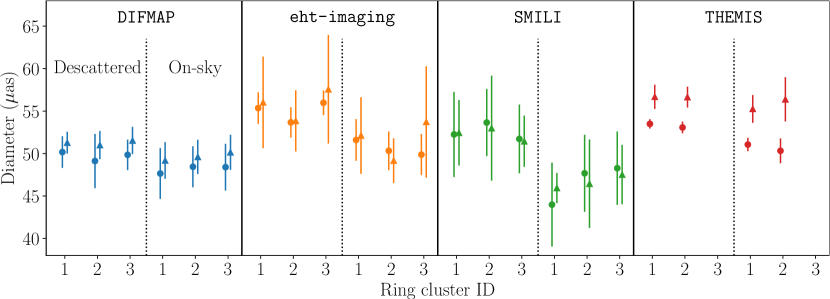
Figure 21: The ring diameters measured from April 7 images, shown separately for each cluster with a ring morphology, each pipeline, and descattered or on-sky reconstructions. Circle and triangle points and associated error bars indicate the means and standard deviations of diameters measured with REx and VIDA, respectively. Note that Themis error bars appear significantly smaller than the error bars on DIFMAP, eht-imaging, and SMILI. This is partly due to the fact that Themis is primarily quantifying aleatoric (e.g., statistical) uncertainty whereas the goal of the other imaging surveys is to also characterize epistemic (e.g., systematic) uncertainty.

In this subsection, we present ring parameter results only for images from ring morphology clusters (Figure 13). In Figure 21, we show the diameters measured for on-sky and descattered ring images for each pipeline. We find that the ring images are consistent with a diameter of $\sim$50 $\mu$as, as shown for each ring morphology cluster separately in Section 7.2 and Figure 14.

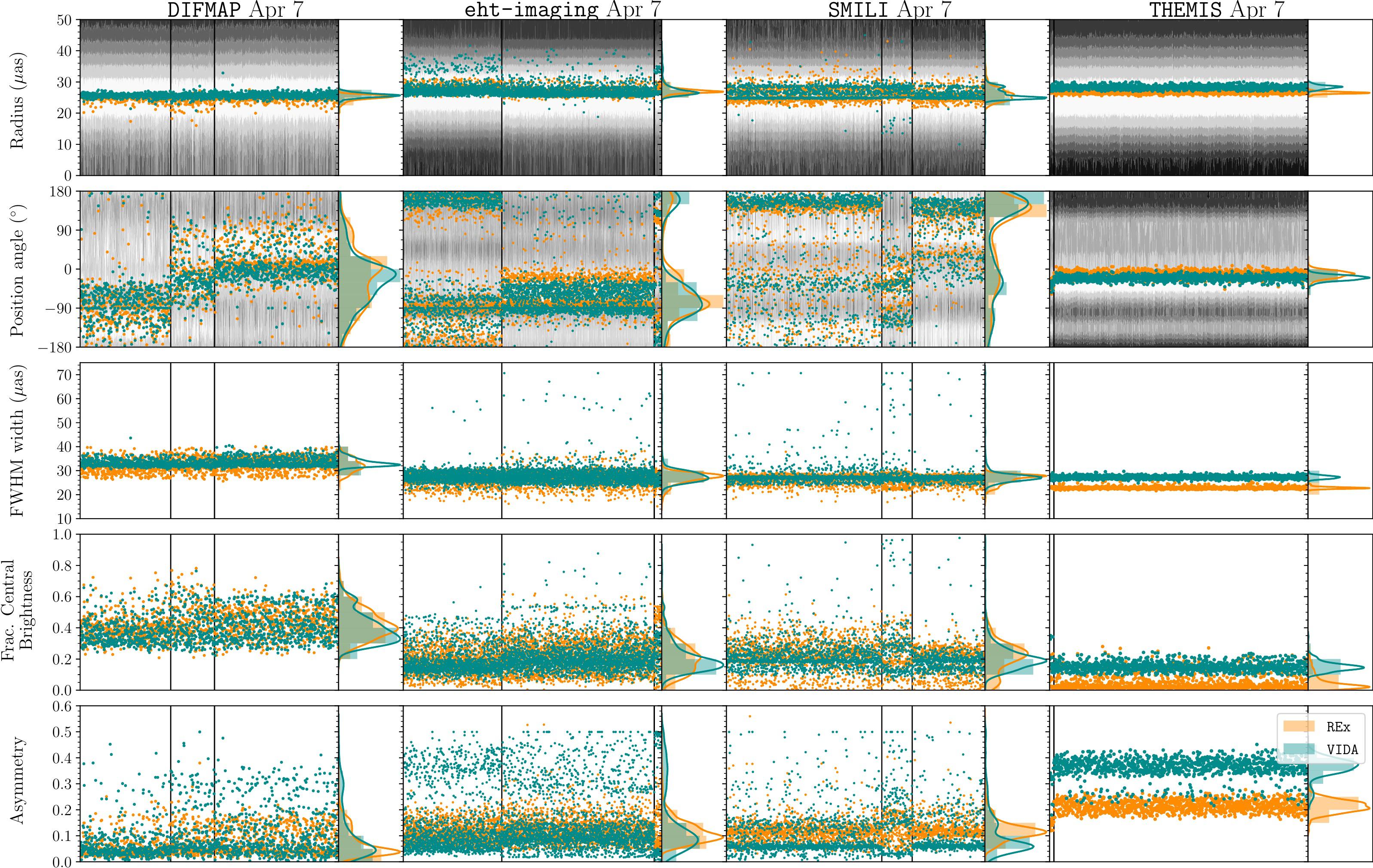
Figure 22: Ring fit results for Sgr A* Top Set descattered images in the ring clusters reconstructed from April 7 data. Each panel shows the distribution of ring parameters corresponding to the images resulting from a single pipeline. In each panel, the scatter plot on the left shows a ring parameter extracted from each image using REx (orange) and VIDA (green); the vertical histogram on the right shows the resulting kernel density estimation from the collection of extracted image parameters. Images are ordered by clusters described in Section 7.2, of which boundaries are shown with vertical solid lines. From left to right, the panels show the results for DIFMAP, eht-imaging, SMILI and Themis. For the radius and position angle, we also show the radial/azimuthal brightness distribution of each image in the background.

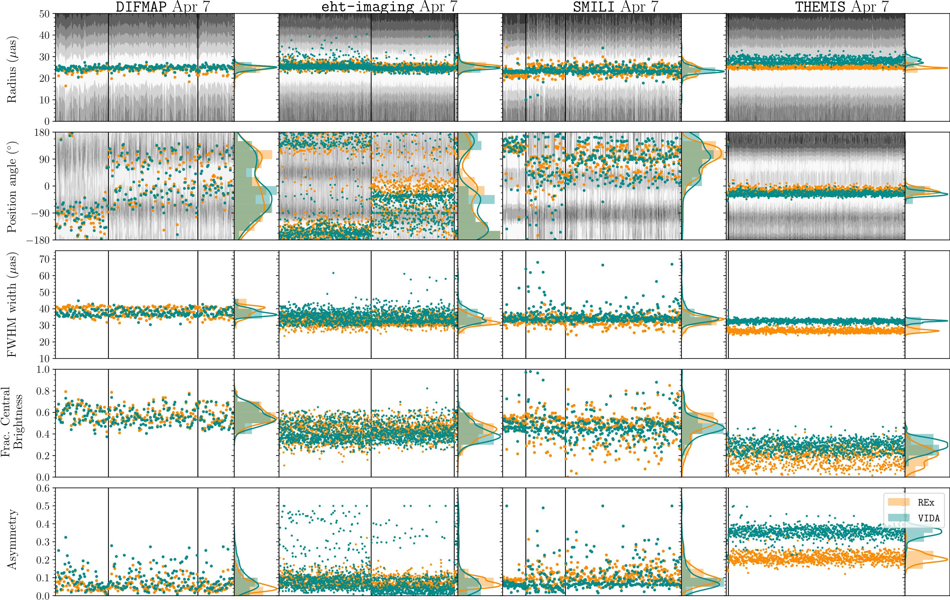
Figure 23: Ring fit results for Sgr A* Top Set on-sky images reconstructed from April 7 data. Refer to the caption of Figure 22 for more detail.

For more detailed distributions of ring parameters, in Figure 22 we show the ring parameter fitting results of Sgr A^∗ descattered Top Set or posterior images for April 7. From top to bottom, distributions of ring radius, position angle, ring width, fractional central brightness, and asymmetry are presented for four pipelines. Results from both REx and VIDA are shown, and for comparison azimuthally or radially averaged brightness distributions are shown in the background of diameter $d$ and position angle $\eta$ plots.

Radius distributions are clearly peaked at $\sim$ 25 $\mu$as and mostly concentrated between 25 and 30 $\mu$as, being consistent across the three pipelines. Note that in some occasions, REx and VIDA show discrepancy in the radius (and some other parameters), which is mostly due to the difference of the responses to an image with a salient feature. However, as seen in the kernel density distributions of the radius, contributions of such outliers are negligible for determinations of the mean ring radius. Meanwhile, the PA value is by far less consistent across the pipelines or even within a single pipeline. Multiple modes clearly appear in the Top Set images with various PA values, as already seen in Section 7. Note that the scatter of PAs tends to be larger when the ring has multiple bright spots that affect the resulting PA, or when the azimuthal profile is close to uniform without a clear peak. Ring width values are $\sim 30\ \rm{\mu as}$, and this may come from the angular resolution of the observation. Fractional central brightness is mostly $\sim 0-0.3$ for RML and Themis while minor non-ring modes (right-most clusters in each panel) tend to show somewhat higher values. These values confirm that majority of the images show ring-like structures with clear central depression. CLEAN images tend to have a slightly larger value of width and central brightness than RML and Themis, as expected due to the beam-convolution effect for CLEAN imaging. Asymmetry values are $\sim 0.1$, indicating that most of Sgr A^∗ images have a nearly symmetric azimuthal intensity distribution on ring. Apart from time variability, Sgr A^∗’s apparent symmetry could be one of possible reason for difficulty in constraining the PA.

Figure 23 shows the ring parameter fitting results of the on-sky Top Set or posterior images. Comparing the ring parameters with and without scattering mitigation, PA values are slightly different and FWHM and fractional central brightness values are larger for the on-sky images. These differences are reasonable when one considers the angular broadening effect due to scattering that remains in on-sky images. On the other hand, radius and asymmetry show similar distributions between descattered and on-sky images – we obtain a ring diameter of $\sim$50 $\mu$as for on-sky images, indicating that the ring size is robust with little dependence on the scattering correction.

In Table 7, we summarize the mean diameters and their standard deviations over the ring images reconstructed by each pipeline for both descattered and on-sky images and on both April 6 and 7. As seen in the table, the mean ring radii for on-sky images are slightly smaller than those of the descattered cases by a few $\mu$as. This small reduction of ring radii is mainly due to the difference of effective resolutions with/without scattering mitigation. Nevertheless, the ring radii are within their standard deviations and thus broadly consistent regardless of scattering mitigation.

Comparing the results of April 6 and 7 in Table 7, diameters derived from ring reconstructions are consistent within the computed standard deviations, regardless of the pipelines. The other parameters (except for PA) also give consistent values for both days. Again, PA values have a large scatter in April 6 images; the existence of large scatter in PA indicates that it is difficult to constrain the azimuthal brightness distributions along the ring. In general, most of the Top Set images show a ring morphology with a consistent diameter around $\sim$50 $\mu$as.

In Appendix I we list the fitted diameter, width, position angle, asymmetry, and fractional central brightness measured for each one of the identified imaging clusters and different pipelines shown in Figure 22 and Figure 23.

Table 7: Mean and standard deviation of diameter $d$ and width $w$ measured from Top Set or posterior Sgr A^∗ images for each pipeline.

Descattered $d\ \rm{(\mu as)}$ $w\ \rm{(\mu as)}$ DIFMAP April 6 Ring REx $46\pm 4.1$ $33\pm 3.5$ VIDA $51\pm 3.1$ $33\pm 3.1$ April 7 Ring $49\pm 2.1$ $32\pm 2.9$ $51\pm 1.5$ $33\pm 1.7$ eht-imaging April 6 Ring $56\pm 4.5$ $24\pm 2.4$ $59\pm 11.3$ $30\pm 10.4$ April 7 Ring $54\pm 2.0$ $26\pm 2.6$ $54\pm 4.6$ $27\pm 3.5$ SMILI April 6 Ring $57\pm 3.4$ $24\pm 1.9$ $46\pm 12.0$ $50\pm 16.6$ April 7 Ring $52\pm 4.7$ $26\pm 2.1$ $52\pm 4.0$ $27\pm 4.7$ Themis April 6 Ring $51\pm 3.9$ $25\pm 1.2$ $54\pm 0.9$ $24\pm 0.9$ April 7 Ring $53\pm 0.7$ $22\pm 0.5$ $56\pm 1.2$ $27\pm 0.7$

On-sky $d\ \rm{(\mu as)}$ $w\ \rm{(\mu as)}$ DIFMAP April 6 Ring REx $46\pm 3.0$ $34\pm 4.3$ VIDA $47\pm 1.9$ $39\pm 3.4$ April 7 Ring $48\pm 2.7$ $38\pm 2.7$ $49\pm 2.1$ $37\pm 2.0$ eht-imaging April 6 Ring $49\pm 3.9$ $28\pm 3.6$ $50\pm 5.6$ $41\pm 6.7$ April 7 Ring $50\pm 2.5$ $32\pm 2.7$ $50\pm 4.1$ $35\pm 3.8$ SMILI April 6 Ring $43\pm 0.4$ $28\pm 3.1$ $39\pm 3.9$ $46\pm 8.8$ April 7 Ring $47\pm 4.7$ $33\pm 2.7$ $47\pm 3.8$ $35\pm 5.2$ Themis April 6 Ring $46\pm 2.1$ $30\pm 1.6$ $47\pm 3.1$ $33\pm 2.0$ April 7 Ring $50\pm 1.5$ $26\pm 1.1$ $56\pm 2.6$ $32\pm 0.9$

9 Short-timescale Dynamic Properties on Select Observation Window

The dynamical timescale at the location of the innermost stable circular orbit for Sgr A^∗, $t_{\rm g}=12\pi\sqrt{6}GM/c^{3}$ for zero spin, is approximately 30 min and can be smaller by a factor of $\sim 10$ if the black hole is spinning rapidly. Variability at these timescales across the electromagnetic spectrum, including at 230 GHz, is one of Sgr A* salient features – see Wielgus et al. (2022) and references therein. As discussed in Section 3.2 and Paper II, a few EHT closure phase triangles show measurable variability across the 2017 observing campaign that can be attributed to intrinsic source variability. In this section, we explore the level and characteristics of structural changes in the Sgr A^∗ image that are consistent with the observed variability.

Recovering time-resolved structures on these short timescales is especially challenging due to the sparse snapshot $(u,v)$-coverage for the EHT array. Indeed, without additional constraints, any observed change in the visibility domain can be interpreted as caused either by intrinsic variability or simply by the rotation of the baselines with the Earth and their probing of different spatial structures – though fitting fast fluctuations in the visibilities with static emission requires larger fields-of-view. This is especially true for baselines that probe regions of the $(u,v)$-space in which the visibility amplitudes show deep minima (or nulls), across which the complex visibilities change by order unity over infinitesimal changes in baseline length.

In attempts to describe the EHT observations with a static image, we assign any observed variation to spatial structures and mitigate potential effects of variability by inflating the error budget. In this section, we instead attempt to fit the time-evolving data directly to produce spatially- and temporally-resolved images of Sgr A^∗ on minute timescales. Our analysis of dynamic properties presuppose that the 230 GHz emission from Sgr A^∗ is compact (see Section 2.3) and ring-like such that the short-timescale variability we see can be attributed to changes in the image with time. We combine two independent analysis methods – dynamic imaging with temporal regularization between frames and snapshot geometric modeling – to identify trends in the spatial evolution of Sgr A^∗.

Our analysis shows that significant uncertainty exists in any attempt to characterize the spatially-resolved dynamics of Sgr A^∗ using EHT 2017 data. We expect that future observations with an expanded EHT array will yield significantly improved time- and spatially-resolved movies of Sgr A^∗.

9.1 Selecting an Observation Window

The rotation of the Earth causes the EHT’s snapshot $(u,v)$-coverage to change over time. Static imaging and modeling approaches assume the source is unchanging in time, which allows these approaches to combine data from a full night of observations. However, recovery of short-timescale evolution requires that we only consider coverage synthesized on the variability timescale. This “snapshot" coverage is extremely sparse and introduces artifacts into image reconstructions. To minimize these artifacts, we constructed and evaluated metrics to assess the performance of the snapshot coverage and identify the most promising time windows for dynamic analysis. These metrics rely purely on the $(u,v)$-coverage rather than the properties of the underlying Sgr A^∗ visibilities. The construction and validation of a suite of these metrics are reviewed in Farah et al. (2021).

We consider metrics that assess several attributes of the $(u,v)$-coverage, including the largest gap in coverage (Wielgus et al. 2020), the fraction of the $(u,v)$ plane covered (Palumbo et al. 2019), and the geometric properties of the coverage (Farah et al. 2021). We summarize the application of these metrics to the 2017 April 7 EHT Sgr A^∗ data set in Appendix J. These three metrics identify a period from approximately 1.5-3.2 GMST on April 6 and 7 that maximally mitigates the EHT’s snapshot coverage limitations. During this time window, all sites participate in observing Sgr A^∗ except PV, though there is a notable dropout of the LMT between approximately 2.4-2.9 GMST on both days. All dynamic analyses discussed in the remainder of Section 9 are performed only in this selected time window.

Figure 24 shows the $(u,v)$-coverage for April 7 during the roughly 100 min observation window selected for dynamic analysis, along with the coverage for a single 60 second “snapshot" integration. Closure phases from two informative triangles are overlaid for April 6 and 7 during this time window. These closure phases show distinct evolution in the resolved structure of Sgr A^∗ during the same 100 min window on April 6 and 7.

9.2 Dynamic Imaging and Modeling Methods

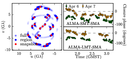
Figure 24: (Left) $(u,v)$-coverage for the selected time window for dynamic imaging and modeling. The light blue points show the coverage of the full night of observation, while the dark blue points and the red points represent the coverage for the selected dynamic imaging region and a single 60s snapshot from that region, respectively. (Right) Closure phases for Sgr A^∗ (green and yellow) on two representative triangles during the selected time region.

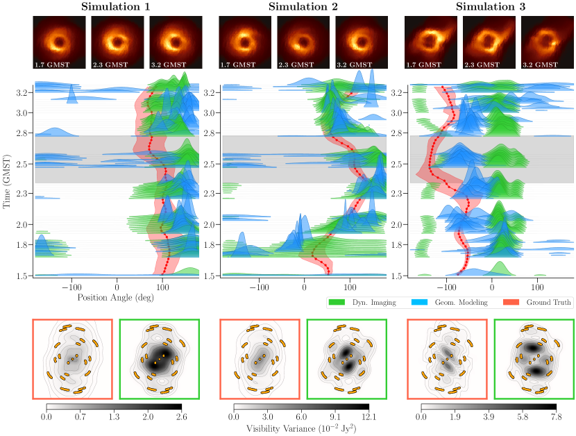
Figure 25: Position angle (PA) recovered from synthetic data from three different GRMHD simulations on April 7 EHT coverage during the dynamic analysis window using both StarWarps dynamic imaging and DPI snapshot geometric modeling techniques. (Top row) Ground truth GRMHD movie snapshots (including interstellar scattering) from each of the three simulations at 1.7, 2.3, and 3.2 GMST. (Middle row) Plots of PA vs time for the reconstructions compared with the simulation ground truth (in red). The shaded red region indicates the circular standard deviation of the ground truth PA computed using REx (refer to Section 8 and Chael (2019)). Modeling histograms (blue) correspond to actual marginal posterior distributions, whereas for StarWarps imaging the histograms represent the distribution of PAs and their associated uncertainties for a collection of movies reconstructed under different parameter settings. The gray band at roughly 2.6 GMST indicates the time period where the LMT dropped out of the observation. (Bottom row) Visibility variance in the $(u,v)$ plane over the selected time window for the ground truth simulation movies (left, red) and the reconstruction (right, green). In Simulations 1 & 2, both dynamic imaging and snapshot geometric modeling methods are often able to correctly identify the PA of evolving GRMHD movies during this time window, but they show significant offsets from the correct PA in Simulation 3. From left to right, the maximum variance of the ground-truth (reconstructed) movie is 0.85 (2.62), 4.45 (12.07), and 3.94 (7.79) $\times 10^{-2}$ Jy². Contours start at 90% of the peak variance and decrease by successive factors of 2 until they reach 0.7%.

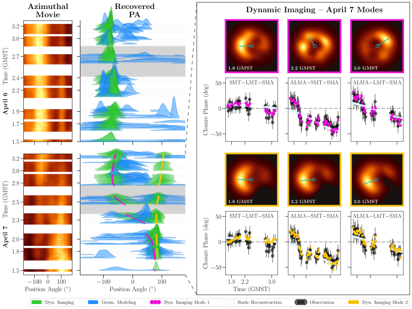
Figure 26: (Left) Mean azimuthal brightness profiles from the StarWarps movie reconstructions, unwrapped around the ring as a function of time, and PA distributions obtained from dynamic imaging and snapshot geometric modeling reconstructions of EHT Sgr A^∗ data on April 6 (top) and 7 (bottom) in the selected time window. Geometric modeling distributions are marginal PA posteriors from DPI. Imaging histograms represent the distribution of PAs and their associated uncertainties from a collection of StarWarps movies reconstructed under different parameter settings with the spatial prior mean $\mu$ and temporal regularization $\beta_{Q}^{-1}$ held fixed (refer to Equation 7). Blank spaces indicate time regions without any data. The gray band at roughly 2.6 GMST indicates the region where the LMT dropped out and data coverage is poor. Both dynamic imaging and modeling appear to identify a nearly constant PA on April 6 but a variable PA over the same time window on April 7. In the reconstructions in this figure, both dynamic imaging and modeling make a prior assumption that the source morphology is ring-like; StarWarps imaging uses a prior/initialization image of a uniform ring, while geometric modeling uses a second order $m$-ring ($m=2$) model. Both dynamic imaging and modeling recover “descattered" movies using the J18model1 refractive noise model.
(Right) Focus on the two modes reconstructed by StarWarps on April 7. For each mode, the top panels show three reconstructed snapshots at different times, and bottom panels compare the fitting of the corresponding reconstructed movie (magenta or yellow) and a representative static reconstruction from the eht-imaging static imaging pipeline (white) to the closure phase data measured by three key triangles. The dynamic reconstruction on the top (magenta) shows an evolving PA shift over the observation window. In contrast, the reconstruction on the bottom has a nearly constant PA of $\sim 100^{\circ}$ (yellow). In the selected closure phase plots (bottom rows), the measured data is averaged in 60 s snapshots and the error bars do not include a variability noise model. The static image visibilities (white) capture the general trend of the data, but they do not well fit variability in the closure phases. In contrast, both selected StarWarps dynamic reconstructions better fit the data on minute timescales. We find that the fit’s behavior on the SMT-LMT-SMA triangle has a large influence on the resulting PA of the movie on April 7. A positive SMT-LMT-SMA closure value tends to result in a southeast PA ($\sim 100^{\circ}$) whereas a negative value results in a more northwest PA ($\sim-80$^∘).

To analyze Sgr A^∗’s spatially-resolved dynamics during the 100 min selected region of time on April 6 and 7, we use two methods: dynamic imaging and snapshot geometric modeling (also simply referred to as dynamic modeling). Both methods fit EHT 2017 data on 60s snapshot integrations within the selected observation window but make different prior assumptions about the structure of the source in space and time. Note that unlike in static imaging, we do not flux normalize the data before dynamic analysis. Because the $(u,v)$-coverage is sparse even in the best available time window, both methods need to make strong prior assumptions about the spatial and/or temporal structure of the source to constrain the fits to the data. Note that when performing dynamic imaging/modeling fits we do not include a variability noise budget as is done in static imaging (Section 3.2.2).

Dynamic Imaging

Dynamic imaging methods reconstruct a time-evolving image that best fits the observed evolution of Sgr A^∗. Our dynamic imaging approach is based on StarWarps (Bouman et al., 2018), which enforces continuity across an image and in time by means of spatial and temporal regularization (Section 4.4.2). Temporal regularization is set by a parameter $\beta_{Q}^{-1}$ which corresponds to the allowed variance between pixels in snapshots that are typically 60s apart; smaller values of $\beta_{Q}^{-1}$ correspond to stronger continuity in time. Spatial regularization is imposed by a multivariate Gaussian prior on snapshots with a mean $\mu$ and covariance $\Lambda$ that encourages spatial smoothness (see Equation 7 and Bouman et al. 2018). We examine the sensitivity of time-variable image features (e.g., position angle) to different settings in the StarWarps imaging algorithm by running surveys over different values of the spatial regularization covariance $\Lambda$ and data weights of the visibility amplitude and log closure amplitude; we typically keep $\beta_{Q}^{-1}$ and the mean image $\mu$ fixed and examine the sensitivity of our results to these parameters separately across different surveys. Unless specified otherwise, in this paper we set $\beta_{Q}^{-1}$ to $5\times 10^{-6}$ (Jy/pixel)² and the prior mean $\mu$ and initialization image to an image of a uniform ring blurred by a 25 $\mu$as beam. These surveys result in distributions of the image features at each snapshot in time. For each of the measurements obtained from 54 parameter combinations, we draw 100 random samples from a normal distribution characterized by the image feature measurement and its associated error. These survey results are not posterior probability distributions, but they do provide a sense of the robustness of the sensitivity of movie reconstructions to changes in the algorithm parameters.

Geometric modeling

In our geometric modeling approach, a simple geometric model is fit to each 60 s snapshot independently, with no enforced correlations in time. We consider several different $m$-ring models (Johnson et al., 2020), described by infinitesimally thin rings with azimuthal brightness variations decomposed into Fourier modes, which are subsequently blurred with a circular Gaussian kernel. The complexity of an $m$-ring model depends on the maximum number of Fourier modes, $m$, that are added (e.g. $m=1$ corresponds to a simple crescent). To model a central floor we include a Gaussian that is located at the center of the ring; the size and brightness of the Gaussian are additional model parameters.

For each $m$-ring model considered, we produce a multi-dimensional posterior using two modeling approaches. First, we consider a variational inference based approach, DPI, that fits to the log closure amplitudes and closure phases (Sun & Bouman, 2021; Sun et al., 2022). Second, we consider a sampling based method, Comrade (Tiede, 2022), which fits to visibility amplitudes and closure phases. Comrade uses the nested sampling package dynesty (Speagle, 2020) and the probabilistic programming language Soss (Scherrer & Zhao, 2020). The different data products used by DPI and Comrade imply different assumptions made about the telescope amplitude gains – they are unconstrained in DPI, while in Comrade the gain amplitudes are more constrained and are included as model parameters during fitting (see Paper IV). As a result of these different data products, DPI and Comrade produce slightly different posteriors. Details of the geometric modeling approaches are further explained in Paper IV.

Comparing dynamic imaging & modeling

Both dynamic imaging and modeling share a common goal of extracting time- and spatially-resolved structure in Sgr A^∗ but there are key differences between the methods in how prior assumptions about the spatial and temporal variability are incorporated. StarWarps imaging allows for more freedom in the recovered spatial structure but assumes strong temporal regularization between frames. In contrast, snapshot geometric modeling is restricted to a parameterized set of spatial structures, but makes no assumptions on image correlations in time. Although snapshot geometric modeling cannot recover spatial structures outside of the $m$-ring model specifications, it allows for quantifying the uncertainty in $m$-ring model features (and their temporal variability) as it estimates full posterior distributions for the particular geometric model used.

Diagnostics

To characterize our dynamic reconstructions, we mostly investigate trends of the brightness position angle (PA; see Eq. 21 in M87^∗ Paper IV) with time. The PA is a simple and easily characterizable feature of the brightness distribution around an asymmetric ring. For Starwarps reconstructed movies, we extract the ring PA on the different snapshots using REx; in $m-$ring model fitting results, the PA is obtained directly from the fitted model as the argument of the first azimuthal Fourier mode.

Ring assumption

Many of the results in this section apply strong prior assumptions that Sgr A^∗’s underlying structure is ring-like, motivated by the ring morphology recovered in static image reconstructions using the full $(u,v)$-coverage (Section 7). StarWarps reconstructions enforce a ring constraint by setting the mean prior image $\mu$ to a ring with $\approx 50\,\mu$as diameter and a width set by a circular Gaussian blurring kernel. In geometric modeling, the ring assumption is intrinsically imposed by the structure of the $m$-ring model. In Section 9.4.1 and in Appendix J we explore the sensitivity of our results to the choice of mean image $\mu$ in StarWarps.

9.3 Synthetic Data Tests

Sparse snapshot $(u,v)$-coverage can lead to artifacts in both imaging and geometric modeling results. These artifacts appear in static imaging, but are further amplified in dynamic imaging due to the far-sparser coverage  (Farah et al., 2021). Thus, it is important to assess how the sparse $(u,v)$-coverage during the selected time window may affect the recovered results and whether it may introduce biases in recovered image features, particularly the position angle (PA) of ring-like images.

9.3.1 Static Crescents

In Section J.3 we present synthetic data tests conducted to characterize the effect of the sparse snapshot EHT2017 $(u,v)$-coverage on PA recovery from static crescent images. These tests show that there are significant biases in the recovered PA from 60s snapshots when the brightness asymmetry of the ground truth ring image is low. When there is a strong asymmetry in the brightness distribution around the ring, however, the PA is accurately recovered even with 60s snapshot $(u,v)$-coverage.

9.3.2 GRMHD Simulations

We explored how our methods perform in recovering time-varying position angles from three selected GRMHD simulation movies. We used three representative GRMHD movies from the GRMHD library presented in Paper V (see Section 5.2). We generated visibility data from the three movies over the 100 min dynamic analysis window on April 7 using the same procedure described in Section 5, including atmospheric noise, telescope gain errors, and polarimetric leakage.

Figure 25 presents results obtained from both dynamic imaging and modeling reconstructions of these three synthetic data sets. The ground truth simulation PA evolution is recovered (with $\sim$30^∘) for the first two models (Simulation 1 & 2). However, there are several localized deviations in the recovered PA distributions from the ground truth in these models, especially when the the instantaneous $(u,v)$-coverage worsens (e.g. during the LMT dropout time region). For the third model (Simulation 3) both the dynamic imaging and modeling methods recover significant offset from the true PA. One potential cause of this offset is the prominent extended jet structure to the northwest of the ring in the SANE simulation. This extended structure cannot be captured in either the dynamic imaging or modeling methods due to their strong prior assumptions of a ring-like morphology.

In the bottom row of Figure 25, we investigate the complex variance of the Fourier transform of the reconstructed images across the selected time window for both the ground truth (scattered) movies and the reconstructions. We find that in all three cases the reconstructions tend to introduce more variability than is present in the ground truth. In Simulation 1 and 2 this excess variability does not prevent the reconstructions from qualitatively recovering the correct PA trend, but the PA results are not correctly recovered in Simulation 3.

These results indicate that although we often recover the PA accurately from some realistic synthetic GRMHD data sets, we should remain cautious when interpreting Sgr A^∗ dynamic results. Our methods sometimes incorrectly recover the PA, especially if extended structure is present that is not captured by the prior assumptions on the source structure made by the dynamic imaging and modeling methods. In addition to effects from extended structure, there may be additional uncharacterized systematic uncertainty from prior assumptions in the reconstructions in these results derived from extremely sparse snapshot Sgr A^∗ coverage.

9.4 Sgr A^∗ Spatiotemporal Characterization and Uncertainty

Here we present results of our analysis on Sgr A^∗’s spatially resolved temporal variability on minute timescales on April 6 and 7, using both dynamic imaging and snapshot geometric modeling methods. In Figure 26, we show detailed results for the Sgr A^∗ PA evolution and data fits reconstructed using a restricted range of dynamic imaging and modeling parameters. In Figure 27 we show PA results obtained under a broader range of parameter settings.

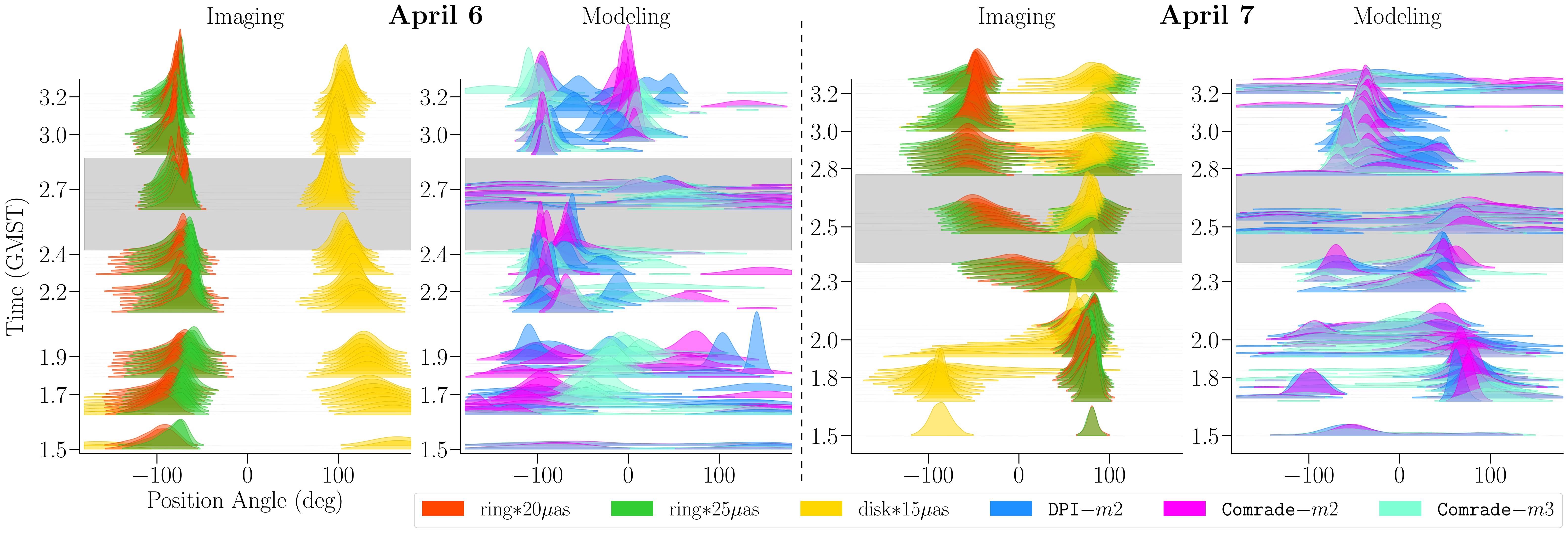
Figure 27: The PA for the 2017 Sgr A^∗ data recovered using dynamic imaging and geometric modeling techniques under different assumptions. StarWarps imaging results were obtained using a spatial prior image set to either a uniform ring convolved with a circular Gaussian kernel with FWHM of 20 or 25 $\mu$as (see Figure 7), or a uniform disk blurred with a kernel with FWHM of 15 $\mu$as. Descattered modeling results were obtained from geometric models with increasing complexity ($m$-ring 2 vs $m$-ring 3) and different fitting software packages (DPI vs Comrade). All results were obtained from low-band data on April 6 and 7 that has been descattered with a J18model1 refractive noise floor. The gray band at roughly 2.6 GMST indicates the region where the LMT has dropped out and data coverage is poor.

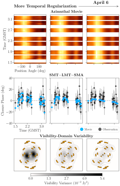
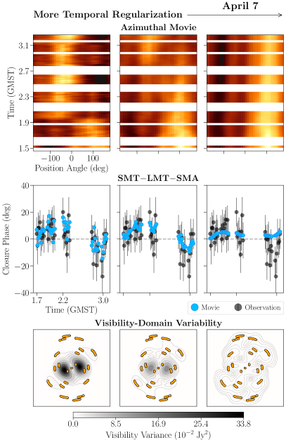
Figure 28: Comparing the effect of temporal regularization on the reconstructed StarWarps movies for April 6 and 7. The temporal regularization strength is increased from left to right ($\beta_{Q}^{-1}=5\times 10^{-4}$, $5\times 10^{-6}$, and $5\times 10^{-8}$ (Jy/pixel)²). For each value of $\beta_{Q}^{-1}$, we show the mean unwrapped movie around the ring (top), the mean closure phase values on the triangle SMT-LMT-SMA (middle), and the variance of the complex visibilities across the $(u,v)$ plane (bottom). As temporal regularization is increased the recovered movies become more static, and the degree of $(u,v)$ plane variability decreases. From weak to strong regularization, the maximum variance of the reconstructed movie is 5.37, 1.11, and 0.73 $\times 10^{-2}$ Jy² on April 6, and 33.81, 13.24, and 0.50 $\times 10^{-2}$ Jy² on April 7. Contours start at 90% of the peak variance and decrease by successive factors of 2 until they reach 0.7%. For comparison, the variance in the light curve over this interval is ${\sim}0.5\times 10^{-2}{\rm Jy}^{2}$. Thus, the leftmost reconstruction with the weakest temporal regularization produces a movie with visibility variance substantially exceeding the light curve variance due to overfitting to the thermal noise.

In general, we find that snapshot geometric modeling results performed under different $m$-ring orders, scattering mitigation strategies, and modeling codes produce fairly consistent results. The modeling results show broad posteriors of PA at each 60 s snapshot but still indicate significant differences between April 6 and 7 and between the first and second halves of the 100 min window on April 7. In rough terms, the PA on April 6 is centered around $\sim-50^{\circ}$, with some scatter around this value over the time window. In contrast, on April 7 the modeling results show PA posteriors that are initially centered around $\sim 90^{\circ}$ and then shift to values centered around $\sim-50^{\circ}$ in the second half of the time window.

Compared to snapshot geometric modeling, dynamic imaging allows for more freedom in spatial and temporal regularization, and as a result is more sensitive to parameter choices. Dynamic imaging results can produce movies that reproduce the PA trends on April 6 and 7 recovered by snapshot modeling. These PA trends – a stable PA on April 6 and a shifting PA on April 7 – are predominantly seen in dynamic imaging reconstructions with low temporal regularization and ring-like spatial priors. Geometric modeling makes similar assumptions, imposing no temporal regularization and enforcing ring structure in the form of the model. In Figure 26, we directly compare dynamic modeling and imaging results under these strong assumptions.

Even in the limited space of dynamic imaging reconstructions conducted with weak temporal regularization and ring-like mean prior images, the imaging results are sensitive to other hyperparameters. In particular Figure 26 indicates that we recover two modes of position angle evolution on April 7 even with the mean prior image and temporal regularization level fixed. We present representative snapshots and fit to the closure phase data from these two modes in the right panels of Figure 26.

When the ring-like mean image prior is changed or the weak temporal regularization is increased in StarWarps dynamic imaging, significantly different PA variations can be recovered from the same data. In Figure 27, we show that when the ring assumption is relaxed and a disk prior is used in reconstruction, StarWarps results show drastically different PA trend over time. In particular, in reconstructions initialized with a disk prior, the PA curves on April 6 and 7 appear to be flipped by $180^{\circ}$ (i.e., on April 7 the PA transitions from $\sim 90^{\circ}$ to $\sim-50^{\circ}$). We further show in Figure 28 that when using stronger temporal regularization in the StarWarps dynamic imaging, the PA stays constant, eliminating the shift from positive to negative PA trend on April 7. We discuss these tests further in the Section 9.4.1 and Section J.5.

Note that April 6 and 7 have nearly identical $(u,v)$-coverage during the selected 100 min region of time. We can thus compare the results obtained over these two days to help disentangle effects of $(u,v)$-coverage from any effects due to intrinsic evolution. If the PA trends that we recover are due primarily to biases from the $(u,v)$-coverage, we would expect to recover the same PA trends on both days. However, we consistently see different PA trends with time using the same parameter settings in both dynamic imaging and modeling methods. This implies that differences in the visibilities, not the $(u,v)$-coverage, drive differences in the PA evolution we see on the two nights in some reconstructions, but it does not help select among any of the different reconstruction modes on either day.

9.4.1 Effect of Model and Imaging Choices

The PA evolution recovered with dynamic imaging and modeling methods is sensitive to choices made in the imaging and modeling procedures that enforce constraints on the spatial and temporal structure of the reconstructions. Enforcing strong spatial or temporal priors will suppress any structural variability while adding too much flexibility in a model with sparse data constraints will lead to overfitting or uninformative posteriors. In Section J.5 we present in detail several tests of these choices for both imaging and modeling methods; here, we highlight the most important results.

Spatial Priors

Constraints on the spatial structure are enforced via the $m$-ring order in geometric model fitting and via the choice of mean image prior in dynamic imaging. To test the effects of different mean prior images in StarWarps, we produced reconstructions using uniform ring priors with increasing widths (from convolution of the ring described in Section 5 with circular beams of 11, 15, 20, and 25 $\mu$as FWHM; henceforth ring$\textasteriskcentered$11$\mu$as, ring$\textasteriskcentered$15$\mu$as, ring$\textasteriskcentered$20$\mu$as, and ring$\textasteriskcentered$25$\mu$as priors, respectively). We also used a tapered disk with diameter $\sim$ 74$\mu$as (see Figure 7) as a prior that does not feature any central dip. The disk is tapered via convolution with a circular beam of 15 $\mu$as (henceforth, disk$\textasteriskcentered$15$\mu$as prior). We discuss the details of these prior choices in Section J.5.1. For geometric modeling, we tested ring-like models of increasing complexity in their azimuthal brightness distribution, from crescent models ($m=1$) to higher order $m$-rings. When fitting $m$-rings to Sgr A^∗ snapshot data, we explored $m$ from 1 to 4 and selected the order to use based on the Bayesian evidence across all data sets – settling on $m=2$ (see Section J.5.2).

Figure 27 shows histograms of the dynamic imaging PA results made using different mean prior images and PA posterior distributions from geometric modeling results from different $m-$ring orders. We also compare modeling results from two different modeling codes in Figure 27. The reconstructed PA trends are fairly consistent on both days among the different $m$-ring orders in geometric model fitting. In StarWarps imaging, reconstructions using ring-like mean prior images of several different thicknesses produce similar trends, with a stable PA on April 6 and a PA transition from positive to negative values on April 7. However, when a disk prior is used in StarWarps the PA trends of both April 6 and 7 change drastically and appear to be flipped by $180^{\circ}$. Figure 44 in Appendix J shows image snapshots and data fits for StarWarps reconstructions with both disk and ring mean prior images. Note that although the position angle evolution is different than the movie reconstructed using a ring prior, the movie reconstructed with a disk prior still results in a ring-like structure, though with a less prominent central brightness depression.

Temporal Regularization

Geometric modeling enforces no correlations in between temporal snapshots, while dynamic imaging can enforce correlations via temporal regularization. Figure 28 shows that when using stronger temporal regularization in StarWarps (lower values of $\beta^{-1}_{Q}$) the PA becomes constant in time on both April 6 and 7 – a result of the method enforcing strong continuity between frames. Note that in the case of high temporal regularization, the SMT-LMT-SMA closure triangle fits in the second half of the time window on April 7 appear offset with respect to the data, although still within two standard deviations of most data points.

We also show that reconstructions with low levels of temporal regularization produce prominent variance in the model visibilities plane at $(u,v)$ points that are not sampled by our coverage during this time window. In contrast, reconstructions with more temporal regularization lower the overall variance of model visibilities everywhere in the Fourier plane and place the peaks in the variance maps at $(u,v)$ points sampled by the EHT. We discuss the interpretation of the different temporal regularization values $\beta^{-1}_{Q}$ used here in Section J.2 and further tests of the StarWarps temporal regularization further in Section J.5.1.

Scattering

Another choice made in both dynamic imaging and modeling procedures common to both static and dynamic reconstruction methods is the strategy for mitigating the effects of interstellar scattering in Sgr A^∗ data. We investigate the effects of the same five prescriptions for scattering mitigation we use in static imaging on the dynamic reconstructions in Section J.4. In general, we find that choices made in the scattering mitigation procedure contribute less to our overall uncertainty than choices related to the spatial prior or temporal regularization.

9.5 Sgr A^∗ Dynamic Property Conclusions

Our aim in this section has been to use the 2017 EHT data to explore spatially-resolved dynamics of Sgr A^∗ on minute timescales. First, we identified the time windows with the best $(u,v)$-coverage during the observation run – a roughly 100 min window on April 6 and 7. We identify a significant difference between the closure phases on April 6 and 7, signifying that the underlying structure is different on the two days. We reconstruct movies from this small slice of the EHT data using dynamic imaging and geometric snapshot modeling methods. We track the average position angle (PA) in our dynamic imaging and modeling results as a way of following a specific, dynamic, and measurable aspect of the source over time. We find that we are able to recover the PA in synthetic EHT data from some GRMHD simulation movies; however, there are prominent cases when this is not the case and both geometric modeling and dynamic imaging methods recover biased results.

On April 6, most dynamic imaging and modeling results show a stable PA in the Sgr A^∗ images over the selected window. In contrast, the recovered PA evolution on April 7 is more dependent on prior assumptions on the spatial structure and temporal regularization. On April 7, when using a ring image as a spatial prior and weak temporal regularization, dynamic imaging results largely align with geometric modeling results and show an evolution in the PA of $\sim 140^{\circ}$ over the $\sim 100$ min window. However, we also see several other PA trends in the dynamic imaging results, including a PA evolution in the opposite direction and modes where the PA is static on both days.

These results, along with our synthetic data tests, show that while the 230 GHz image of Sgr A^∗ may exhibit interesting and measurable dynamics, our current methods cannot conclusively determine the PA evolution of Sgr A^∗. Dynamic reconstructions of Sgr A^∗ with EHT2017 coverage should thus be interpreted with caution. This analysis provides a promising starting point for further studies of future evolution seen in Sgr A^∗ EHT observations with denser $(u,v)$-coverage.

10 Summary and Conclusions

We present Sgr A^∗ static and dynamic imaging results for data taken with the EHT in April 2017. Sgr A^∗ was observed with eight EHT stations at six geographic sites over five observing days, out of which the highly sensitive phased ALMA array participated in April 6, 7, and 11. April 7 is the only day in which the easternmost station PV participated, providing the best $(u,v)$-coverage that probes a null at $\sim$3.0 G$\lambda$. On April 11 Sgr A^∗ exhibits the highest variability in the light curve during the 2017 campaign (Wielgus et al., 2022), possibly related to an X-ray flare observed shortly before the start of the EHT observations (Paper II), rendering static imaging for this day particularly challenging. For these reasons, April 7 has been used as the primary dataset, while April 6 is considered as a secondary data set. Results from the remaining 2017 EHT observations of Sgr A^∗ will be presented in future publications.

Similar to the 2017 EHT observations of M87^∗ (; ; ; ; ; ), the data sets analyzed in this paper are the first with sufficient sensitivity and $(u,v)$-coverage to reconstruct images of Sgr A^∗ on event-horizon scales with an angular resolution of $\sim$20 $\mathrm{\mu as}$. Imaging Sgr A^∗ with the EHT is however significantly more challenging than M87^∗ due to the interstellar scattering towards the Galactic Center, and most importantly the rapid intra-day variability that characterizes Sgr A^∗, with timescales much shorter than the duration of our typical EHT observing runs.

To mitigate the scattering effects in our Sgr A^∗ reconstructions we have developed a strategy based on Fish et al. (2014), Psaltis et al. (2018) and Johnson et al. (2018) to account for the angular broadening and substructure induced by diffractive (Section 3.1.1) and refractive (Section 3.1.2) scattering, respectively. Images of Sgr A^∗ have been obtained with and without these scattering mitigation prescriptions to asses their impact in our reconstructions.

It is however the rapid intra-day intrinsic variability of Sgr A^∗, coupled with the sparse $(u,v)$-coverage as compared with regular VLBI observations, that poses the strongest challenge for reconstructing horizon-scale images of Sgr A^∗ with the EHT. With a typical variability timescale of a few minutes, the horizon-scale brightness distribution can change significantly during our typical multi-hour observing runs, which violates the fundamental assumption for Earth rotation VLBI aperture synthesis. To overcome this extraordinary challenge we have included a “variability noise budget" in the observed visibilities (Section 3.2.2) that facilitates the reconstruction of static full-track images capturing the time-averaged structure.

Static full-track imaging of Sgr A^∗ has been conducted through surveys over a wide range of imaging assumptions using the classical CLEAN algorithm (implemented in DIFMAP), regularized maximum likelihood methods (eht-imaging and SMILI), and a Bayesian posterior sampling method (Themis), as described in Section 4. Imaging surveys, exploring $\sim$10^3-5 parameter combinations, were first performed on synthetic data sets designed to be qualitatively consistent with Sgr A^∗ measurements, including its characteristic temporal variability (Section 5). The use of synthetic data sets allows us to asses the capability to accurately reproduce different morphologies with our imaging methods, and to select the “Top Sets": imaging parameter combinations for RML and CLEAN methods that successfully reproduce the known ground truth movies (Section 6.2.2).

Unlike for M87^∗, where a persistent ring structure is observed across imaging pipelines (M87^∗ Paper IV), our static reconstructions of Sgr A^∗ show structural changes within and across the different imaging methods used. The variety of images can be classified into four main clusters of images corresponding to ring images with three different azimuthal brightness distributions, and a cluster that contains a small number of non-ring images with multiple morphologies. This classification is resilient to the scattering mitigation prescription used, including no mitigation.

Although the relative fraction of non-ring images in the Top Set reconstructions from RML and CLEAN is very small ($\leq$5% in the April 7 descattered images), we note that the Top Sets do not sample from the Bayesian posterior likelihood and are instead meant to characterize the range of possible images due to epistemic uncertainty. On the other hand, the full Bayesian imaging approach implemented in the Themis pipeline does provide a Bayesian posterior exploration that characterizes aleatoric uncertainty. Scattering mitigated Sgr A^∗ reconstructions from Themis for April 7 only contain ring images with a very similar structure as that found for RML and CLEAN methods, although it also identifies a small number (2%) of on-sky non-ring images (Section 7).

The April 6 data set suffers from poorer $(u,v)$-coverage and likely more unusual intrinsic variability. This results in April 6 reconstructions that contain a less prominent ring structure in the RML and CLEAN pipelines. Nonetheless, the diameter of the ring structures recovered for April 6 are consistent with that of the April 7 ring images. In addition, although descattered Themis samples of April 6 primarily show a corrupted ring or non-ring structure, Themis posterior samples for the combined April 6 and 7 data sets exhibits only clear ring-like images for both, the on-sky and scattered mitigated reconstructions.

Imaging of a synthetic GRMHD data set with data properties similar to those of Sgr A^∗ and characterized by a ring image of $\sim$50 $\mu$as (Section 6.4.2) shows similar imaging results to those found in Sgr A^∗: RML and CLEAN methods recover ring images with different azimuthal orientations and a small ($\leq 5\%$ ) Top Set fraction of non-ring images, while Themis posterior sample only recovers ring images.

We conclude that the Event Horizon Telescope Sgr A^∗ data show compelling evidence for an image that is dominated by a bright ring of emission. This conclusion is based on our extensive analysis of the effects of sparse $(u,v)$-coverage, source variability and interstellar scattering, as well as studies of simulated visibility data, which find that non-ring images are recovered in the minority by our imaging pipelines for variable sources with an intrinsic ring morphology (Section 7.5). Representative first event horizon-scale images of Sgr A^∗ are shown in Figure 13, obtained from the April 7 data set by averaging similar Top Set and posterior images together. Despite the different azimuthal brightness distributions observed, all ring images have a ring diameter of $\sim$50 $\mu$as on both April 6 and 7, consistent with the expected “shadow" of a $4\times 10^{6}M_{\odot}$ black hole in the Galactic Center located at a distance of 8 kpc.

We also present preliminary dynamic imaging and modeling analysis of Sgr A^∗ on horizon scales in an attempt to characterize the azimuthal variations on minute timescales and their uncertainties. We applied dynamical analysis methods to a 100-minute interval of the 2017 Sgr A^∗ data with the best coverage on April 6 and 7. On April 6, most dynamic imaging and modeling methods recover a stable position angle. In contrast, on April 7 the recovered PA evolution is more dependent on spatial and temporal regularization; April 7 frequently shows an evolving position angle over the 100 minute window when we impose strong priors on the spatial structure but weak temporal regularization. However, when expanding the parameter space available to the imaging and modeling methods, we recover disparate modes in the position angle behavior, including some reconstructions that are nearly static. Our initial results show that significant uncertainty exists in any attempt to characterize the spatially-resolved dynamics of Sgr A^∗ using sparse EHT 2017 data, but this analysis provides a promising starting point for further dynamical studies of Sgr A^∗ with future EHT observations.

EHT.

We thank the anonymous referee for helpful suggestions that improved this paper.

The Event Horizon Telescope Collaboration thanks the following organizations and programs: the Academia Sinica; the Academy of Finland (projects 274477, 284495, 312496, 315721); the Agencia Nacional de Investigación y Desarrollo (ANID), Chile via NCN$19\_058$ (TITANs) and Fondecyt 1221421, the Alexander von Humboldt Stiftung; an Alfred P. Sloan Research Fellowship; Allegro, the European ALMA Regional Centre node in the Netherlands, the NL astronomy research network NOVA and the astronomy institutes of the University of Amsterdam, Leiden University and Radboud University; the ALMA North America Development Fund; the Black Hole Initiative, which is funded by grants from the John Templeton Foundation and the Gordon and Betty Moore Foundation (although the opinions expressed in this work are those of the author(s) and do not necessarily reflect the views of these Foundations); Chandra DD7-18089X and TM6-17006X; the China Scholarship Council; China Postdoctoral Science Foundation fellowship (2020M671266); Consejo Nacional de Ciencia y Tecnología (CONACYT, Mexico, projects U0004-246083, U0004-259839, F0003-272050, M0037-279006, F0003-281692, 104497, 275201, 263356); the Consejería de Economía, Conocimiento, Empresas y Universidad of the Junta de Andalucía (grant P18-FR-1769), the Consejo Superior de Investigaciones Científicas (grant 2019AEP112); the Delaney Family via the Delaney Family John A. Wheeler Chair at Perimeter Institute; Dirección General de Asuntos del Personal Académico-Universidad Nacional Autónoma de México (DGAPA-UNAM, projects IN112417 and IN112820); the Dutch Organization for Scientific Research (NWO) VICI award (grant 639.043.513) and grant OCENW.KLEIN.113; the Dutch National Supercomputers, Cartesius and Snellius (NWO Grant 2021.013); the EACOA Fellowship awarded by the East Asia Core Observatories Association, which consists of the Academia Sinica Institute of Astronomy and Astrophysics, the National Astronomical Observatory of Japan, Center for Astronomical Mega-Science, Chinese Academy of Sciences, and the Korea Astronomy and Space Science Institute; the European Research Council (ERC) Synergy Grant “BlackHoleCam: Imaging the Event Horizon of Black Holes" (grant 610058); the European Union Horizon 2020 research and innovation programme under grant agreements RadioNet (No 730562) and M2FINDERS (No 101018682); the Generalitat Valenciana postdoctoral grant APOSTD/2018/177 and GenT Program (project CIDEGENT/2018/021); MICINN Research Project PID2019-108995GB-C22; the European Research Council for advanced grant ‘JETSET: Launching, propagation and emission of relativistic jets from binary mergers and across mass scales’ (Grant No. 884631); the Institute for Advanced Study; the Istituto Nazionale di Fisica Nucleare (INFN) sezione di Napoli, iniziative specifiche TEONGRAV; the International Max Planck Research School for Astronomy and Astrophysics at the Universities of Bonn and Cologne; DFG research grant “Jet physics on horizon scales and beyond” (Grant No. FR 4069/2-1); Joint Princeton/Flatiron and Joint Columbia/Flatiron Postdoctoral Fellowships, research at the Flatiron Institute is supported by the Simons Foundation; the Japan Ministry of Education, Culture, Sports, Science and Technology (MEXT; grant JPMXP1020200109); the Japanese Government (Monbukagakusho: MEXT) Scholarship; the Japan Society for the Promotion of Science (JSPS) Grant-in-Aid for JSPS Research Fellowship (JP17J08829); the Joint Institute for Computational Fundamental Science, Japan; the Key Research Program of Frontier Sciences, Chinese Academy of Sciences (CAS, grants QYZDJ-SSW-SLH057, QYZDJSSW-SYS008, ZDBS-LY-SLH011); the Leverhulme Trust Early Career Research Fellowship; the Max-Planck-Gesellschaft (MPG); the Max Planck Partner Group of the MPG and the CAS; the MEXT/JSPS KAKENHI (grants 18KK0090, JP21H01137, JP18H03721, JP18K13594, 18K03709, JP19K14761, 18H01245, 25120007); the Malaysian Fundamental Research Grant Scheme (FRGS) FRGS/1/2019/STG02/UM/02/6; the MIT International Science and Technology Initiatives (MISTI) Funds; the Ministry of Science and Technology (MOST) of Taiwan (103-2119-M-001-010-MY2, 105-2112-M-001-025-MY3, 105-2119-M-001-042, 106-2112-M-001-011, 106-2119-M-001-013, 106-2119-M-001-027, 106-2923-M-001-005, 107-2119-M-001-017, 107-2119-M-001-020, 107-2119-M-001-041, 107-2119-M-110-005, 107-2923-M-001-009, 108-2112-M-001-048, 108-2112-M-001-051, 108-2923-M-001-002, 109-2112-M-001-025, 109-2124-M-001-005, 109-2923-M-001-001, 110-2112-M-003-007-MY2, 110-2112-M-001-033, 110-2124-M-001-007, and 110-2923-M-001-001); the Ministry of Education (MoE) of Taiwan Yushan Young Scholar Program; the Physics Division, National Center for Theoretical Sciences of Taiwan; the National Aeronautics and Space Administration (NASA, Fermi Guest Investigator grant 80NSSC20K1567, NASA Astrophysics Theory Program grant 80NSSC20K0527, NASA NuSTAR award 80NSSC20K0645); NASA Hubble Fellowship grant HST-HF2-51431.001-A awarded by the Space Telescope Science Institute, which is operated by the Association of Universities for Research in Astronomy, Inc., for NASA, under contract NAS5-26555; the National Institute of Natural Sciences (NINS) of Japan; the National Key Research and Development Program of China (grant 2016YFA0400704, 2017YFA0402703, 2016YFA0400702); the National Science Foundation (NSF, grants AST-0096454, AST-0352953, AST-0521233, AST-0705062, AST-0905844, AST-0922984, AST-1126433, AST-1140030, DGE-1144085, AST-1207704, AST-1207730, AST-1207752, MRI-1228509, OPP-1248097, AST-1310896, AST-1440254, AST-1555365, AST-1614868, AST-1615796, AST-1715061, AST-1716327, AST-1716536, OISE-1743747, AST-1816420, AST-1935980, AST-2034306); NSF Astronomy and Astrophysics Postdoctoral Fellowship (AST-1903847); the Natural Science Foundation of China (grants 11650110427, 10625314, 11721303, 11725312, 11873028, 11933007, 11991052, 11991053, 12192220, 12192223); the Natural Sciences and Engineering Research Council of Canada (NSERC, including a Discovery Grant and the NSERC Alexander Graham Bell Canada Graduate Scholarships-Doctoral Program); the National Youth Thousand Talents Program of China; the National Research Foundation of Korea (the Global PhD Fellowship Grant: grants NRF-2015H1A2A1033752, the Korea Research Fellowship Program: NRF-2015H1D3A1066561, Brain Pool Program: 2019H1D3A1A01102564, Basic Research Support Grant 2019R1F1A1059721, 2021R1A6A3A01086420, 2022R1C1C1005255); Netherlands Research School for Astronomy (NOVA) Virtual Institute of Accretion (VIA) postdoctoral fellowships; Onsala Space Observatory (OSO) national infrastructure, for the provisioning of its facilities/observational support (OSO receives funding through the Swedish Research Council under grant 2017-00648); the Perimeter Institute for Theoretical Physics (research at Perimeter Institute is supported by the Government of Canada through the Department of Innovation, Science and Economic Development and by the Province of Ontario through the Ministry of Research, Innovation and Science); the Spanish Ministerio de Ciencia e Innovación (grants PGC2018-098915-B-C21, AYA2016-80889-P, PID2019-108995GB-C21, PID2020-117404GB-C21); the University of Pretoria for financial aid in the provision of the new Cluster Server nodes and SuperMicro (USA) for a SEEDING GRANT approved towards these nodes in 2020; the Shanghai Pilot Program for Basic Research, Chinese Academy of Science, Shanghai Branch (JCYJ-SHFY-2021-013); the State Agency for Research of the Spanish MCIU through the “Center of Excellence Severo Ochoa” award for the Instituto de Astrofísica de Andalucía (SEV-2017- 0709); the Spinoza Prize SPI 78-409; the South African Research Chairs Initiative, through the South African Radio Astronomy Observatory (SARAO, grant ID 77948), which is a facility of the National Research Foundation (NRF), an agency of the Department of Science and Innovation (DSI) of South Africa; the Toray Science Foundation; Swedish Research Council (VR); the US Department of Energy (USDOE) through the Los Alamos National Laboratory (operated by Triad National Security, LLC, for the National Nuclear Security Administration of the USDOE (Contract 89233218CNA000001); and the YCAA Prize Postdoctoral Fellowship.

We thank the staff at the participating observatories, correlation centers, and institutions for their enthusiastic support. This paper makes use of the following ALMA data: ADS/JAO.ALMA#2016.1.01154.V. ALMA is a partnership of the European Southern Observatory (ESO; Europe, representing its member states), NSF, and National Institutes of Natural Sciences of Japan, together with National Research Council (Canada), Ministry of Science and Technology (MOST; Taiwan), Academia Sinica Institute of Astronomy and Astrophysics (ASIAA; Taiwan), and Korea Astronomy and Space Science Institute (KASI; Republic of Korea), in cooperation with the Republic of Chile. The Joint ALMA Observatory is operated by ESO, Associated Universities, Inc. (AUI)/NRAO, and the National Astronomical Observatory of Japan (NAOJ). The NRAO is a facility of the NSF operated under cooperative agreement by AUI. This research used resources of the Oak Ridge Leadership Computing Facility at the Oak Ridge National Laboratory, which is supported by the Office of Science of the U.S. Department of Energy under Contract No. DE-AC05-00OR22725. We also thank the Center for Computational Astrophysics, National Astronomical Observatory of Japan. The computing cluster of Shanghai VLBI correlator supported by the Special Fund for Astronomy from the Ministry of Finance in China is acknowledged.

APEX is a collaboration between the Max-Planck-Institut für Radioastronomie (Germany), ESO, and the Onsala Space Observatory (Sweden). The SMA is a joint project between the SAO and ASIAA and is funded by the Smithsonian Institution and the Academia Sinica. The JCMT is operated by the East Asian Observatory on behalf of the NAOJ, ASIAA, and KASI, as well as the Ministry of Finance of China, Chinese Academy of Sciences, and the National Key Research and Development Program (No. 2017YFA0402700) of China and Natural Science Foundation of China grant 11873028. Additional funding support for the JCMT is provided by the Science and Technologies Facility Council (UK) and participating universities in the UK and Canada. The LMT is a project operated by the Instituto Nacional de Astrófisica, Óptica, y Electrónica (Mexico) and the University of Massachusetts at Amherst (USA). The IRAM 30-m telescope on Pico Veleta, Spain is operated by IRAM and supported by CNRS (Centre National de la Recherche Scientifique, France), MPG (Max-Planck-Gesellschaft, Germany) and IGN (Instituto Geográfico Nacional, Spain). The SMT is operated by the Arizona Radio Observatory, a part of the Steward Observatory of the University of Arizona, with financial support of operations from the State of Arizona and financial support for instrumentation development from the NSF. Support for SPT participation in the EHT is provided by the National Science Foundation through award OPP-1852617 to the University of Chicago. Partial support is also provided by the Kavli Institute of Cosmological Physics at the University of Chicago. The SPT hydrogen maser was provided on loan from the GLT, courtesy of ASIAA.

This work used the Extreme Science and Engineering Discovery Environment (XSEDE), supported by NSF grant ACI-1548562, and CyVerse, supported by NSF grants DBI-0735191, DBI-1265383, and DBI-1743442. XSEDE Stampede2 resource at TACC was allocated through TG-AST170024 and TG-AST080026N. XSEDE JetStream resource at PTI and TACC was allocated through AST170028. This research is part of the Frontera computing project at the Texas Advanced Computing Center through the Frontera Large-Scale Community Partnerships allocation AST20023. Frontera is made possible by National Science Foundation award OAC-1818253. This research was carried out using resources provided by the Open Science Grid, which is supported by the National Science Foundation and the U.S. Department of Energy Office of Science. Additional work used ABACUS2.0, which is part of the eScience center at Southern Denmark University. Simulations were also performed on the SuperMUC cluster at the LRZ in Garching, on the LOEWE cluster in CSC in Frankfurt, on the HazelHen cluster at the HLRS in Stuttgart, and on the Pi2.0 and Siyuan Mark-I at Shanghai Jiao Tong University. The computer resources of the Finnish IT Center for Science (CSC) and the Finnish Computing Competence Infrastructure (FCCI) project are acknowledged. This research was enabled in part by support provided by Compute Ontario (http://computeontario.ca), Calcul Quebec (http://www.calculquebec.ca) and Compute Canada (http://www.computecanada.ca).

The EHTC has received generous donations of FPGA chips from Xilinx Inc., under the Xilinx University Program. The EHTC has benefited from technology shared under open-source license by the Collaboration for Astronomy Signal Processing and Electronics Research (CASPER). The EHT project is grateful to T4Science and Microsemi for their assistance with Hydrogen Masers. This research has made use of NASA’s Astrophysics Data System. We gratefully acknowledge the support provided by the extended staff of the ALMA, both from the inception of the ALMA Phasing Project through the observational campaigns of 2017 and 2018. We would like to thank A. Deller and W. Brisken for EHT-specific support with the use of DiFX. We thank Martin Shepherd for the addition of extra features in the Difmap software that were used for the CLEAN imaging results presented in this paper. We acknowledge the significance that Maunakea, where the SMA and JCMT EHT stations are located, has for the indigenous Hawaiian people.

Appendix A Estimating Static Image Posteriors with Themis

A.1 The Themis Image Model

Themis is a general sampling-based parameter estimation framework developed for comparing parameterized models with the VLBI data produced by the EHT (Broderick et al., 2020a). Implemented within Themis is a wide variety of image models, ranging from phenomenological geometric models (e.g., Gaussians, rings, etc.) to physically motivated ray-traced radiative transfer models (e.g., semi-analytic accretion flow models). Of relevance here is a set of splined raster models, described in detail in Broderick et al. (2020b), and applied to polarized reconstructions in M87^∗ Paper VII. In these, the image reconstruction process is replaced with a model reconstruction problem in which the intensity at control points on a rectilinear raster grid are varied, with the final image produced at arbitrary locations via a cubic spline.

The image model presented in Broderick et al. (2020b) has a fixed field of view in the two cardinal directions. As described in M87^∗ Paper VII, this restriction has been subsequently relaxed, with a more general set of models, adaptive splined rasters, that permit a rotation of the raster and a resizing of the field of view among its principle axes. In this way, not only can the brightness at each control point vary, but the locations of the control points themselves can evolve. This results in a very flexible image model even when the dimension of the raster is small. The splined raster and adaptive splined raster models may be combined with any other Themis models, and typically large-scale features will be absorbed by a large-scale Gaussian component. The dimension of the underlying image model is, then, the sum of the number of control points, $N_{x}\times N_{y}$, two fields of view and the orientation of the raster, and the number of parameters associated with a potential geometric addition.

The Themis model has been fit to a variety of EHT data types. The bulk of the Themis-based analyses presented here employed the light-curve-normalized, LMT-calibrated complex visibilities directly. The residual complex station gains are reconstructed during each model evaluation and marginalized over via the Laplace approximation (see Section 6.8 of Broderick et al., 2020a). Log-normal priors are imposed on the station gain amplitudes with uncertainties that depend on the a priori calibration estimates (see Section 2.2). Network calibrated sites (ALMA, APEX, JCMT, SMA) are assumed to have a log-normal 1$\sigma$ uncertainty of 1%; following the LMT gain amplitude correction it is assumed to have a residual log-normal 1$\sigma$ uncertainty of 20%; and the remaining sites (PV, SMT, SPT) are assigned a log-normal 1$\sigma$ uncertainty of 10%. In this way Themis fully explores the potential station gain space during its exploration of the underlying image space. Some early analyses made use of visibility amplitudes and closure phases. For these the station gain amplitudes were reconstructed in a similar fashion as described above, though with a larger log-normal prior on LMT gain of 100% and 20% on all other stations.

A.2 Scattering and Variability Mitigation

Application of Themis-based imaging methods to Sgr A^∗ is complicated by the presence of the confounding factors described in Section 3. Unless otherwise stated, diffractive scattering is mitigated via the scattering model from Johnson et al. (2018) directly to the model visibilities, i.e., instead of deblurring the data, the model is blurred. Refractive scattering and variability are mitigated via a scheme similar to that described in Section 3.1.2. Unlike the description there, for the Themis analyses, the additional noise terms are treated as parameterized contributions to the visibility uncertainties as described in detail in Georgiev et al. (2021).

Explicitly, the Themis analyses assume that the visibility uncertainties are described by

$$\sigma_{j}^{2}(\sigma_{\rm ref},f,a,b,c,u_{0})=\\ \sigma_{j,\rm th}^{2}+\sigma_{\rm ref}^{2}+f^{2}|V|^{2}+\sigma_{\rm var}^{2}(a,b,c,u_{0}),$$ (A1)

where $\sigma_{j,\rm th}$ is the intrinsic thermal uncertainty, $|V|$ is the measured visibility amplitude, and $\sigma_{\rm var}$ is given in Equation 2. Within this prescription, the $\sigma_{\rm ref}$ is conceptually identical to the Const approach to refractive scattering mitigation described in Section 3.1.2, with the exception that it is not fixed. Similarly, the fractional contribution, $f|V|$ is conceptually identical to the systematic noise term, again with the sole distinction being to treat $f$ as a free parameter.

A.3 Likelihood and Parameter Priors

For analyses that fit the visibility amplitudes and closure phases, the Themis log-likelihood is given by the appropriate combination of log-likelihoods from Sections 6.3 and 6.8 from Broderick et al. (2020a). For analyses that fit the full complex visiblities with the noise modeling, the log-likelihood is

$$\mathcal{L}({\bf p},{\bf q})=\\ -\sum_{\rm data}\bigg{\{}\frac{|\hat{V}_{j}-\hat{V}({\bf u}_{j};{\bf p})|^{2}}{2\sigma_{j}^{2}({\bf q})}+\frac{1}{2}\ln\left[2\pi\sigma_{j}^{2}({\bf q})\right]\bigg{\}},$$ (A2)

where $\{\hat{V}_{j}\}$ is the light-curve-normalized visibility data, ${\bf p}$ are the image-model parameters and ${\bf q}=\{\sigma_{\rm ref},f,a,b,c,u_{0}\}$ are the noise-model parameters. The novel terms on the right are simply the $\sigma$-dependent normalization; while normally constant, in this instance they induce a penalty term that constrains the ${\bf q}$. When descattered, the diffractive scattering kernel is applied to the model, as opposed to deblurring the data, which maintains a consistent treatment of the “noise” model among the descattered and on-sky analyses.

Priors on each of the image model parameters are listed in Table 6. In summary, uninformative logarithmic priors are assumed on the brightness at the control points, the raster size and orientation, and a potential shift from the correlation phase center. Similarly uninformative priors are imposed on the refractive scattering mitigation and systematic uncertainty terms of the noise model. In contrast, informed priors are imposed on the remaining parameters of the noise model, set by the pre-modeling considerations from Georgiev et al. (2021) and applied to Sgr A^∗ in Paper IV. The relevant interquartile ranges are data-set specific, and are listed for the Themis analyses reported here in Table 2 for Sgr A^∗ and the various synthetic data sets in Section 5.

A.4 Reconstructing the Posterior with Themis

Themis provides a number of sampling schemes with which to explore the likelihood surface. The bulk of the Themis-based analyses presented here employ a set of Markov Chain Monte Carlo (MCMC) samplers to explore the large-dimensional parameter space, $\{{\bf p},{\bf q}\}$. To efficiently traverse the prior, identify multiple modes, and rapidly locate the global maximum, Themis makes use of parallel tempering, in which multiple, tempered copies of the likelihood, $\mathcal{L}_{\beta}=\beta\mathcal{L}$ are simultaneously explored; higher “temperature” copies ($\beta\rightarrow 0$) become the reference distribution which we take to be uniform in the prior bounds, while the bottom “temperature” ($\beta=1$) is the posterior to be sampled. These are coupled via the deterministic even–odd swap tempering scheme (Syed et al., 2019), which efficiently moves information through the multiple, tempered levels. Periodically, the $\beta$ are optimized to efficiently move information from the prior to the posterior following the scheme from (Syed et al., 2019). Each individual tempering level is sampled via the Hamiltonian Monte Carlo sampling kernel from the Stan package (Carpenter et al., 2017).

Convergence is assessed via chain statistics, such as, integrated autocorrelation time, approximate split-$\hat{R}$ tests, parameter rank distributions, and visual inspection. Reconstruction quality is determined by inspection of the best-fit sample’s residuals, and “reasonableness” of the associated image and gain reconstructions. Pathological solutions are uncommon, and are typically indicative of poor sampler initialization and/or errors in the input. The number of tempering levels is chosen to exceed the global communication barrier $\Lambda$ (Syed et al., 2019), typically near 20, and is run for $5\times 10^{4}$ to $10^{5}$ MCMC steps per tempering level.

Appendix B Refractive Noise Levels Anticipated for EHT Data

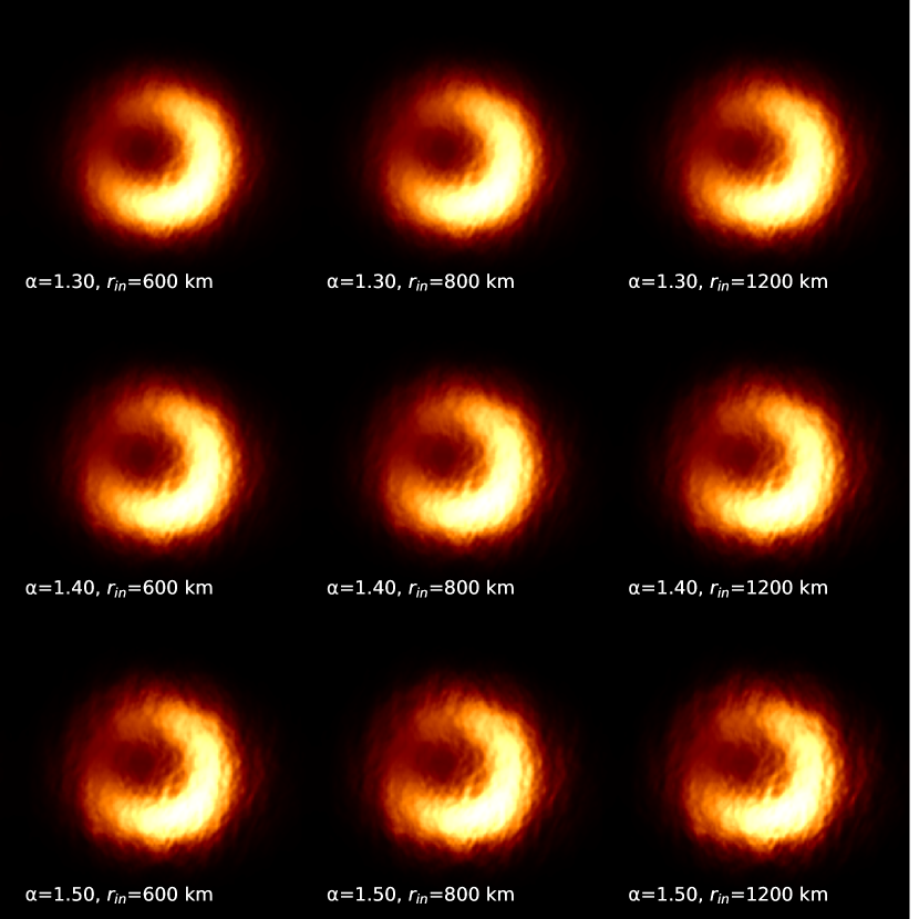
(a) On-sky images

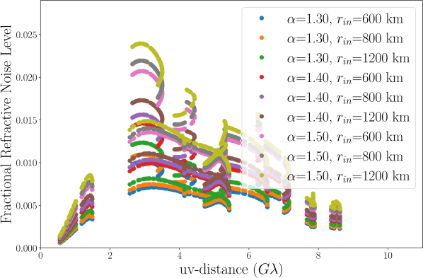
(b) Refractive noise levels

Figure 29: Dependence of refractive substructures on the power-law index $\alpha$ and inner scale of the turbulence $r_{\mathrm{in}}$. (a) Example realizations of the on-sky (i.e., scattered) images of the crescent model in Section 5. Each row shows a realization for a different power-law index $\alpha$ (1.3, 1.4 and 1.5), while each column shows a different $r_{in}$ (600, 800 and 1200 km). (b) The corresponding levels of the flux-normalized refractive noise anticipated for $(u,v)$-coverage of April 7 Sgr A^∗ data. The corresponding normalized visibility amplitudes are shown in Figure 3.

To assess the effects of refractive scattering on our EHT measurements, we use the stochastic optics module implemented in eht-imaging library (Johnson, 2016; Chael et al., 2016). The stochastic optics allows the simulation of scattering realizations for a given intrinsic image and generation of the corresponding synthetic data sets. Here, we focus only on the refractive noise that would affect our imaging, i.e., the substructures on the scattered image. The other effects — centroid shift due to the position wander or total flux modulation— do not affect the image reconstruction of data calibrated by self-calibration and obtained from a single on-sky realization of scattering (Johnson et al., 2018).

The refractive noise level at each $(u,v)$-coordinate is determined by the standard deviation of the flux-normalized visibilities for all realizations, where the centroid of each realization is shifted to the phase center to mitigate the effects of position wander. We adopt a dipole model for the magnetic field wandering in the scattering screen (Johnson et al., 2018). Note that the refractive noise does not depend strongly on the choice of the model for field wander (Psaltis et al., 2018) for the source size anticipated from EHT data and scattering parameters constrained by Johnson et al. (2018).

We first compare the refractive effects for different combinations of the power-law spectral index $\alpha$ of the density fluctuation of the ionized plasma (see Section 3.1.1) and the inner scale of turbulence $r_{in}$. Our refractive noise prescriptions J18model1 and J18model2 are derived with $\alpha=1.38$ and $r_{in}=800\,{\rm km}$, which are the best-fit values in Johnson et al. (2018). These measurements have the uncertainties of $1.3<\alpha<1.5$ and $600\,{\rm km}<r_{in}<1500\,{\rm km}$ (Johnson et al., 2018). Figure 29 shows an example gallery of scattered images and corresponding noise levels in the visibility domain for each combination of $\alpha$ and $r_{in}$ in these ranges. The level of refractive substructure as well as the kernel size of diffractive angular broadening increase with $\alpha$ and $r_{in}$ (Psaltis et al., 2018). Based on the results shown in Figure 29, we adopt a scaling factor of up to 2 to cover the cases of highest refractive noise level in the possible ranges of these two parameters.

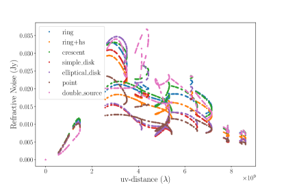
Figure 30: The levels of the flux-normalized refractive noises as a function of $(u,v)$-distance for different intrinsic structures. The refractive noise level is computed on $(u,v)$-coverage of April 7 Sgr A^∗ data. The corresponding normalized visibility amplitudes are shown in Figure 3.

Refractive noise is expected to also be dependent on the intrinsic source structure (e.g. Johnson & Narayan, 2016). To assess this dependence, we estimate the refractive noise levels based on a circular Gaussian and the time-averaged images of the seven geometric models introduced in Section 5.1, for $\alpha=1.38$ and $r_{in}=800\,{\rm km}$. As described in Section 5.1, these geometric models provide a broad consistency with the visibility amplitudes profile of Sgr A^∗ data. The size of the circular Gaussian is adjusted to have the FWHM of 45 $\mathrm{\mu as}$, consistent with the effective FWHMs of other seven geometric models estimated from their second moments. In Figure 30, we show the refractive noise levels for the different intrinsic source models. The refractive noise level is only a few percents of the total flux density regardless of the intrinsic source structures. The standard deviations across different geometric models are typically $\lesssim$0.4% of the total flux density.

J18model2 was derived by taking the mean of the refractive noise levels of seven geometric models. J18model1, on the other hand, is based on the refractive noise level of the the circular Gaussian model. However, the circular Gaussian model has the lowest refractive noise level in the most of $(u,v)$-coverage of Sgr A^∗ data, indicating that the refractive noise level from the circular Gaussian model, if not scaled properly, may underestimate that of Sgr A^∗ data. We derived a scaling factor to make the median of the $\chi^{2}$ of all seven geometric models unity to minimize the effects of its systematically low refractive noise level.

Appendix C First Sgr A^∗ Images from Blind Imaging

Independently performed comparison between synthetic and real observational data can help to identify which image features are likely intrinsic and which are most likely spurious (see this approach in Bouman (2017) for synthetic data and M87^∗ Paper IV for observed EHT data of M87^∗).

To initiate the exploration of possible Sgr A^∗ images while minimizing influence from collective bias, in our first stage of analysis we reconstructed images of Sgr A^∗ in five independent teams. The teams were blind to each others’ work and prohibited from discussing their imaging results. This procedure was similar to that done in M87^∗ Paper IV for first images of M87^∗, with two notable differences. First, since the participants in all teams were already aware of problematic data from previous EHT imaging work, the team activities were not blind to previously-identified problems in the data that could be affecting results. Second, as teams approached the date to submit results it was made known to the organizers that teams would not be comfortable submitting only a single image or movie, and the instructions were changed to submit three representative images or movies per team.

No restrictions were imposed on the data pre-processing or imaging procedures used by each team. Teams 1 and 2 focused primarily on RML methods. Teams 3 and 4 primarily on CLEAN methods. Team 5 used a Bayesian method. All teams used an early-release engineering data set. While the reduction procedures and metadata corresponded to a preliminary version of the calibration pipeline, the data products was deemed mature enough for the blind imaging consistency test. The April 7 data set was selected for the first comparison, as it had the best $(u,v)$-coverage and a very stable light curve over the full observation (Wielgus et al., 2022).

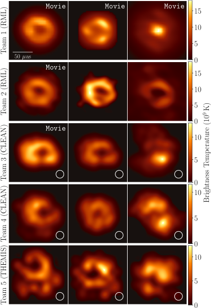
Figure 31: The first EHT images of Sgr A^∗, blindly reconstructed by five independent imaging teams using an early, engineering release of Stokes I data from the April 7 observations. Images from Teams 1 and 2 used RML methods (no restoring beam); images from Teams 3 and 4 used CLEAN (restored with a circular 20 $\mathrm{\mu as}$ beam, shown in the lower right); images from Team 5 used Themis. Each Team shows three representative images from their reconstructions. Some images with the label “Movie” are time-averaged images of movie reconstructions. Many images show ring-like morphology with the diameter of $\sim 50$ $\mathrm{\mu as}$, while some reconstructions show non ring-like morphology. The significant differences in brightness temperature between images are caused primarily by different assumptions regarding the total compact flux density (see Table 8) and also restoring beams applied only to CLEAN and Themis images.

Table 8: Image Properties and Data Consistency Metrics for the First Sgr A* Images

		Team 1	Team 2	Team 3	Team 4	Team 5
Image Properties
Method	Image ID	RML	RML	CLEAN	CLEAN	THEMIS
$F_{\rm cpct}$ (Jy)	1	2.37	2.07	1.90	1.64	1.59
	2	2.38	2.24	1.29	1.18	1.61
	3	2.38	1.99	1.25	0.69	1.73
Engineering Data (10-sec avg., stokes I, 0% sys. error)
$\chi^{2}_{\text{CP}}$	1	2.27 (1.85)	2.35 (1.75)	4.52 (4.20)	2.21	7.78
	2	2.30 (1.81)	2.08	2.51	3.31	6.79
	3	2.81 (1.80)	2.08	2.30	13.80	13.58
$\chi^{2}_{\text{log\,CA}}$	1	3.44 (1.77)	4.67 (2.19)	2.76 (2.98)	2.06	5.90
	2	2.44 (2.07)	2.00	2.49	2.84	4.88
	3	4.73 (2.08)	6.44	2.93	1.91	4.95
Science Release (60-sec avg., Stokes $I$, 0% sys. error)
$\chi^{2}_{\text{CP}}$	1	5.55 (2.53)	6.09 (1.96)	25.05 (21.77)	4.58	54.11
	2	6.08 (2.32)	3.89	7.27	12.11	45.09
	3	8.78 (2.31)	4.11	5.73	108.88	109.10
$\chi^{2}_{\text{log\,CA}}$	1	7.12 (1.52)	10.75 (1.69)	8.31 (5.92)	2.79	24.22
	2	4.02 (1.46)	2.81	5.43	9.66	19.94
	3	6.47 (1.79)	16.95	8.21	7.45	10.01
Science Release (60-sec avg., Stokes $I$, 10% sys. error)
$\chi^{2}_{\text{CP}}$	1	2.42 (1.33)	2.62 (1.18)	7.80 (6.92)	2.32	10.24
	2	2.41 (1.25)	2.09	2.85	5.93	8.02
	3	4.24 (1.17)	2.07	2.56	13.59	16.69
$\chi^{2}_{\text{log\,CA}}$	1	3.36 (0.74)	4.73 (0.89)	3.98 (2.86)	1.32	10.70
	2	1.89 (0.76)	1.26	2.49	3.88	7.55
	3	3.57 (0.88)	6.88	3.72	3.59	4.66

^† $F_{\rm cpct}$, $\chi^{2}_{\text{CP}}$, and $\chi^{2}_{\text{log\,CA}}$ mean the compact total flux density of the VLBI scale images, $\chi^{2}$ to closure phases and log closure amplitudes, respectively. For movies, the values in the parentheses show $\chi^{2}$ to the original movies, while the values outside of them show $\chi^{2}$ to the time-averaged images.

Figure 31 shows images of the three representative submissions made by each team for Sgr A^∗. In cases where dynamic movie reconstructions of Sgr A^∗ were submitted, we show the time-averaged image and indicate that the original submission was a movie. Although most submissions contain flux with a $\sim$50 $\mathrm{\mu as}$ separation, not all submissions contain a clear ring feature. Additionally, of the submissions that do contain a ring feature, the azimuthal flux distribution varies drastically. For example, Team 1 submitted three movies: one containing a ring with a position angle of $\sim 30^{\circ}$, another containing a ring with position angle of $\sim-70^{\circ}$, and the third containing no ring at all.

This initial imaging stage indicated that a $\sim$50 $\mathrm{\mu as}$ feature was likely to exist in the image, but there is significant uncertainty in the presence of a ring structure, as well as the flux distribution around a possible ring structure. In Table 8, we show $\chi^{2}$ values to closure phases ($\chi^{2}_{\rm CP}$) and log closure amplitudes ($\chi^{2}_{\rm\log CA}$) for both engineering data used for imaging and science release data described in Section 2, as well as the compact total flux densities ($F_{\rm cpct}$). There are no significant differences seen in $\chi^{2}$ values of images regardless of the presence of a ring structure and between different azimuthal intensity distributions of the ring structure. These ambiguous results motivated a series of systematic tests to identify if source evolution (similar to that expected to be present in Sgr A^∗) could explain the multiple solutions recovered.

Appendix D Imaging Pipelines

D.1 DIFMAP Pipeline

For this second stage of the imaging process we developed a scripted version of CLEAN in DIFMAP (version higher than 2.5k), together with a python wrapper used over the script, for carrying out an extensive parameter search. The initial manual CLEAN analysis (see Appendix C) together with the pre-imaging considerations (see Section 3) provided the set and range of parameters to be explored on both the synthetic data sets (described in Section 5) and the actual April 6 and 7 Sgr A^∗ data, processed with both fringe fitting pipelines HOPS and CASA, with high and low bands combined.

Prior to CLEAN imaging, the EHT data was pre-processed using the pre-imaging pipeline discussed previously. This includes intra-site normalization to the Sgr A^∗ light curve, coherent averaging of the visibilities using 10 and 60 seconds, the inclusion of an additional systematic error by a factor of 0, 2, and 5%, and the scattering and noise mitigation prescriptions with the common parameters listed in Section 6.1 (see also, Table 3).

The first step in the DIFMAP imaging process is the gridding of the visibilities in the $(u,v)$-plane, that was done by using two different approaches: uniform and natural weighting. The next step is to down-weight the data on all baselines to phased-ALMA in the self-calibration process. As found for the case of M87 (M87^∗ Paper IV), this prevents the ALMA baselines to dominate the phase and amplitude self-calibration process due to their significantly higher S/N. We have tested scaling factors for ALMA baselines weights during self-calibration of 0.1 and 0.5.

Atmospheric fluctuations at the short wavelength of 1.3 mm severely limit the S/N and the capability to reliably measure the visibility phases. We therefore rely on the closure phase measurements and the reconstruction of station phases using the Cornwell Wilkinson hybrid phase self-calibration approach. However the self-calibration with CLEAN model solely relies on the visibility phases and amplitudes, which forces an initial self-calibration of the phases (visibility amplitudes are much better constrained; Paper II), a process which is anchored on the more robustly measured closure phases.

To mitigate any possible bias in our choice for the initial model to self-calibrate the phases, and therefore to minimize the chances of reaching a local minimum in our manifold of image models, we have explored different initial models for the first phase self-calibration. The “fiducial” initial model has been chosen, based on the reduced-$\chi^{2}$ of closure phases with the first reconstructed CLEAN model after the phase self-calibration with the initial model among three different types: a Gaussian with a FWHM of 15 $\mu$as (i.e., unresolved symmetric model), a uniform disk with a size ranging between 56 and 84 $\mu$as (in steps of 4 $\mu$as), and a uniform ring with sizes ranging between 36 and 68 $\mu$as (also in steps of 4 $\mu$as, no width).

A distinctive feature of CLEAN imaging is the use of masks (also known as cleaning windows) to define the area of the image to be cleaned. For this purpose we used a set of centered circular-disk-shaped CLEAN windows (i.e., with no hole in the middle to avoid any biasing).

The size of the cleaning windows should match the expected emission extend of the imaged source. To avoid introducing any prior bias we have surveyed for a relatively large range of mask sizes, from 80 to 110 $\mu$as, that covers our prior Sgr A^∗ image size constrains (Paper II). We note that due to the limited $(u,v)$-coverage larger masks ($\geq$ 100 $\mu$as) may pick up some emission from the main side-lobe of the interferometer, which may be particularly problematic for the point source model given its diffuse emission, more difficult to recover with the CLEAN algorithm.

Contrary to the case of M87 (M87^∗ Paper IV), we do not expect a large extended missing flux in Sgr A^∗ (Paper II), hence our CLEAN stopping criterion is based on setting a minimum threshold for the relative decrease in the rms of the residual image over the image noise estimated from the visibilities.

As a result, the total number of surveyed parameters has been 1680 for the on-sky data set, and 6720 for descattered data. Note that the descattered results are based on a 4 times larger number of parameters due to the scattering mitigation (i.e., refractive noise floor).

D.2 eht-imaging Pipeline

The eht-imaging software library implements the RML imaging technique described in Section 4.2. As a RML method, a successful image reconstruction is achieved when the proper hyperparameters balance the contribution of the selected data products and regularizers to the minimization of Section 4.4.1. Thus, we designed a framework around our imaging pipeline to explore an extensive range of imaging and data pre-calibration parameters.

The pipeline pre-process the input data following the procedure described in Section 6.1 as a first step. Only low- and high-band light-curve normalized data sets were used for static imaging to minimize the effects of the source variability. We opted for an integration time of 60  s and explored all the non-closing systematic error, scattering and intra-day variability noise budgets tabulated in Table 4. The algorithm is then initialized using a symmetric flat disk image contained in a square-shaped grid of 80$\times$80 pixels, which corresponds to a FOV of 150 $\mathrm{\mu as}$. The disk diameter is surveyed as a parameter with values of 70, 80, and 90 $\mathrm{\mu as}$. Note that, among the different imaging regularizers used in the pipeline, the maximum entropy regularizer (MEM) rewards similarity to a prior image, which in this case is assumed to be equal to the initialization image.

Full closure quantities and visibility amplitudes are used as data products. Contrary to M87^∗, the relative weighting of the visibility amplitudes adopted range from a less to an equally important contribution as closure quantities, since complex station gains were derived from calibrator sources beforehand (see Section 5.1.3 in Paper II). Several imaging regularizers and their relative weighting are employed to constraint on the image properties, such as MEM, total variation (TV), and total squared variation (TSV), which enforce similarity to a prior image and/or smoothness over neighboring pixels, respectively.

Convergence to an optimal image which minimizes Section 4.4.1 is then carried out in an iterative process in which the reconstructed image is blurred using a Gaussian kernel with the FWHM of the array nominal resolution ($\sim$24 $\mathrm{\mu as}$), and then used as initialization for the next one to prevent the algorithm of being caught in local minima. In contrast to the M87^∗ pipeline, no self-calibration was performed to the data, since the $\chi^{2}$ statistics obtained for the output images of just one cycle of this iterative procedure were already good enough.

D.3 SMILI Pipeline

The SMILI imaging pipeline was designed to reconstruct images with RML imaging techniques utilizing three imaging regularizers: weighted-$\ell_{1}$ ($\ell_{1}^{w}$), TV, and TSV, similar to M87^∗ Paper IV. Before the imaging process, both low- and high-band EHT data are pre-processed as described in Section 6.1. First, data are normalized by the time-dependent intra-site flux density, and coherently time-averaged at an integration time of 120 sec. The intra-scan fluctuations in LMT baselines are corrected by self-calibrating the shortest VLBI baseline between SMT and LMT to a circular Gaussian with the total flux density of 1 Jy and the FWHM size of 60 $\mathrm{\mu as}$. Finally, the pipeline applies the parameterized mitigation schemes for the non-closing errors, scattering effects and intra-day variations as described in Section 6.1.

The pipeline reconstructs an image from pre-processed data at both low and high bands jointly with the field of view of $150\ \mu\text{as}$ discretized by 2 $\mathrm{\mu as}$ pixels. Throughout the imaging, the pipeline adopts a prior image of a circular Gaussian with the FWHM size of 140, 160 or 180 $\mathrm{\mu as}$ for $\ell_{1}$ prior. The imaging process consists of in total nine imaging cycles, including a single self-calibration of complex visibilities. Each imaging cycle performs 5000 iterations of the L-BFGS-B algorithm used for the gradient-descent optimization in the SMILI’s image solver.

In the first eight cycles of imaging, the images are reconstructed from visibility amplitudes, closure phases and log closure amplitudes. To account for residual errors in the amplitude calibration, the fractional 5 % and  30 % uncertainties are added in quadrature to the errors of visibility amplitudes on non-LMT and LMT baselines, respectively. The first cycle starts with a circular disk image with a $70\ \mu\text{as}$ diameter with the total flux of 1 Jy, while the later cycles subsequently adopt the image from the previous cycle as the initial image after re-centering its center of the mass and blurring with a $5\ \mu\text{as}$ circular Gaussian.

After the eight cycles of imaging, complex visibilities are self-calibrated with its output image. Since the budgets of scattering and intra-day variations are not fractional to visibility amplitudes, these two budgets will not be properly scaled with gains solved with a self-calibration. Therefore, to reflect these two budgets accurately on self-calibrated data, the SMILI pipeline updates these two budgets added to complex visibilities and closure quantities after self-calibration. Finally, the final image is reconstructed by a single imaging cycle using visibility amplitudes and closure quantities.

D.4 Themis Raster Dimension Survey

The sole hyperparameters in the Themis analyses not self-consistently explored during the construction of the posterior are the raster dimensions, $N_{x}$ and $N_{y}$. While reasonable initial guesses may be made based on the diffraction limit, in practice we employ data-driven method: comparing the Bayesian evidence (or appropriate proxies) of different dimensions (Broderick et al., 2020b).

Due to the computational expense of performing Themis posterior reconstructions, we limit the number of raster surveys performed to three: for the Sgr A^∗ April 6 data, the Sgr A^∗ April 7 data, and the GRMHD synthetic data set presented in Section 6.4.2. Of these, we present only that on the Sgr A^∗ April 7 data here for brevity; surveys on the other data sets were conducted similarly. Furthermore, while we did experiment with $N_{x}\neq N_{y}$, given the apparent symmetry of the Sgr A^∗ image, and not wishing to introduce any potential biases away from symmetry in the model specification, we restrict ourselves here to square rasters, i.e., $N_{x}=N_{y}$.

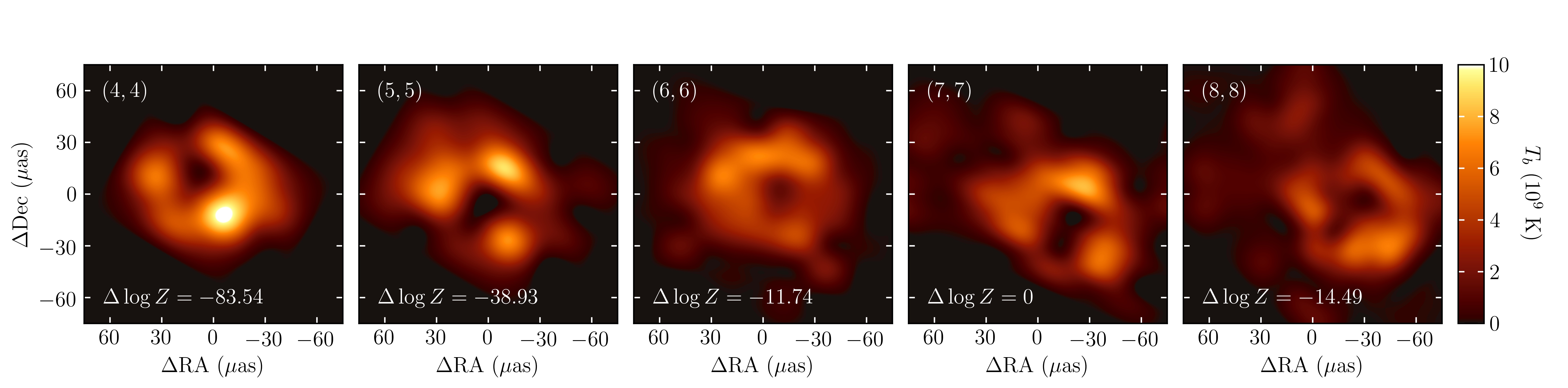
Figure 32: Mean images from the Themis posteriors for $(N_{x},N_{y})=(4,4)$, $(5,5)$, $(6,6)$, $(7,7)$ and $(8,8)$ from left to right. In each the difference in the logarithm of the Bayesian evidence, $\Delta\log Z$, relative to the $(7,7)$ model is listed in the lower left.

Five individual analyses were performed on the April 7, combined high- and low-band complex visibility data as described in Appendix A, differing in the raster dimensions: $(N_{x},N_{y})=(4,4)$, $(5,5)$, $(6,6)$, $(7,7)$ and $(8,8)$. For each, after convergence the Bayesian evidence, $Z$, was computed via thermodynamic integration across tempering levels (Lartillot & Philippe, 2006). Mean images from each analysis and the relative Bayesian evidence are shown in Figure 32.

For raster resolutions that are too small, the fit quality is poor. For raster resolutions that are too large, the added model complexity is not justified by the fit improvement. Importantly, by selecting on $\log Z$, we avoid potential complications associated with the modifications of the likelihood due to noise modeling, correlations between the high- and low-band gains, and non-Gaussianity of the posterior.

As roughly anticipated by the diffraction limit, the preferred raster size is $(7,7)$, which we adopt henceforth. This is accompanied by a convergence of the image structure for raster dimensions of $(5,5)$ and larger. Smaller and larger raster dimensions are overwhelmingly disfavored. Nevertheless, by $(4,4)$ the locations of the knots are identified, though the model misspecification prevents a faithful recovery of their relative brightness.

An identical procedure applied to the Sgr A^∗ April 6 data finds that a smaller $(6,6)$ raster is preferred, ostensibly due to the smaller data volume. Similarly, when applied to the GRMHD synthetic data set in Section 6.4.2, a raster dimension of $(6,6)$ is again preferred, possibly due to the competition between the simplicity of the ring structure.

Appendix E Top Set Selection

E.1 The Effect of Relaxation in $\rho_{NX}$ Criteria

As discussed in Section 6.2, we relaxed the normalized cross-correlation criteria for each image by multiplying the value of $\rho_{NX}$ obtained for $\alpha=24$ $\mathrm{\mu as}$ beam by a relaxation factor of 0.95. This relaxation factor allows us to recover a large enough number of Top Set parameters for evolving synthetic data with Sgr A^∗ $(u,v)$-coverage. This contrasts with the Top Set selection for M87 (M87^∗ Paper IV), where no relaxation factor was considered. The necessity of the relaxation factor originates from the fact that temporal variations of the source structure cause a loss in the image fidelity of the reconstructions.

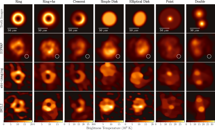
(a) Descattered reconstructions

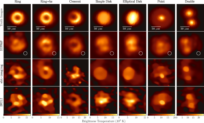
(b) On-sky reconstructions

Figure 33: The worst (i.e., lowest) $\rho_{\rm NX}$ images of synthetic geometric models among those reconstructed from the Top Sets of imaging parameters (a) with and (b) without scattering mitigation.

To ensure that this relaxed criteria is still able to distinguish different morphologies, we show the Top Set images with the worst (i.e. lowest) $\rho_{NX}$ for each geometric model in Figure 33. Each descattered or on-sky reconstruction in Figure 33 shows the image that has the worst $\rho_{NX}$ among the Top Set images for April 7. These images still retain resemblance to the ground truth morphology, demonstrating that Top Set selection with a relaxation factor of 0.95 is still capable of reconstructing the basic structures of synthetic images with varied morphologies.

E.2 $\chi^{2}$ Distribution of Sgr A^∗ Images

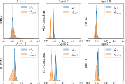
Figure 34: $\chi^{2}$ distributions of the images from each pipeline and epoch which passed the $\rho_{\rm NX}$ criteria. $\chi^{2}$ of closure phases and log closure amplitudes are showed in blue and orange respectively. We assumed $1\ \rm{\%}$ systematic noise and representative variability noise for scattered images and we also added refractive noise when calculating $\chi^{2}$ of deblurred images.

Although the Top Set selection described in Section 6.4.1 is sorely based on the image fidelity of the reconstructions from the synthetic data sets, Top Set images of Sgr A^∗ provide reasonable fits to EHT measurements. In Figure 34, we show $\chi^{2}$ distributions of all the Sgr A^∗ images passing the $\rho_{NX}$ criterion using synthetic data reconstructions. $\chi^{2}$ values were computed for closure phases and log closure amplitudes formed from data after averaged at 1 min, based on the same definition with M87^∗ Paper IV. To account for non-closing effects, refractive scattering and time-variability, we include 1 % of the fractional errors and the representative budgets for scattering and temporal variability (see Section 3.1 and Section 3.2), respectively – in particular, the J18model1 refractive noise model and a variability model with parameters $a=0.02$, $u_{0}=2$, $b=2.5$, and $c=2$ are used. As shown in Figure 34, most of the images have $\chi^{2}$ less than unity, and all the images provide $\chi^{2}<2$, demonstrating that all Top Set images provide reasonable fits to the Sgr A^∗ data within the anticipated deviations of time-variable on-sky images from its intrinsic time-averaged structure. Therefore, we adopt all the parameter sets satisfying the $\rho_{NX}$ criteria as the Top Sets without any cut by $\chi^{2}$.

E.3 Top Sets of Imaging Parameters for April 6

Table 9: Parameters in the DIFMAP Pipeline Top Set on April 6

April 6 (8400 Param. Combinations; 365 in Top Set)
Systematic	0		0.02		0.05
error	15.6%		17.3%		67.1%
$\bf Ref\ Type$	No	Const	2$\times$Const		J18	2$\times$J18
	18.1%	23.0%	14.2%		24.1%	20.5%
$\bf a_{\bf\rm psd}$	No	0.015		0.02		0.025
	21.9%	26.8%		25.8%		25.5%
$\bf b_{\bf\rm psd}$	No	1		3		5
	21.9%	17.3%		24.4%		36.4%
$|u|_{0}$	No			2
	21.9%			78.1%
Time average	10			60
(sec)	49.9%			50.1%
ALMA weight	0.1			0.5
	39.5%			60.5%
UV weight	0			2
	72.6%			27.4%
Mask Diameter	80	85	90	95	100	105	110
($\mathrm{\mu as}$)	10.7%	19.2%	36.2%	17.0%	6.0%	7.9%	3.0%

Note. In each row, the upper line with bold text shows the surveyed parameter value corresponding to the parameter of left column, while the lower line shows the number fraction of each value in Top Set. The total number of surveyed parameter combinations and Top Set are shown in the first row.

Table 10: Parameters in the eht-imaging Pipeline Top Set on April 6

April 6 (112320 Param. Combinations; 1415 in Top Set)
Systematic	0		0.02	0.05
error	19.0%		39.7%	41.3%
$\bf Ref\ Type$	No	Const	2$\times$Const	J18	2$\times$J18
	7.8%	29.2%	26.4%	17.0%	19.6%
$\bf a_{\bf\rm psd}$	No	0.015		0.02	0.025
	13.0%	34.2%		29.4%	23.4%
$\bf b_{\bf\rm psd}$	No	1	2	3	5
	13.0%	16.3%	25.4%	22.1%	23.1%
$|u|_{0}$	No			2
	13.0%			87.0%
TV	$\bf 0$	0.01		0.1	1
	12.4%	27.8%		51.8%	8.0%
TSV	$\bf 0$	0.01		0.1	1
	29.0%	34.8%		35.8%	0.4%
Prior size	70		80	90
($\mathrm{\mu as}$)	15.3%		27.1%	57.6%
MEM	$\bf 0$	0.01		0.1	1
	3.4%	15.3%		77.9%	3.5%
Amplitude	0		0.1	1
weight	0%		4.2%	95.8%

Note. Same as Table 9

Table 11: Parameters in the SMILI Pipeline Top Set on April 6

April 6 (54000 Param. Combinations; 292 in Top Set)
Systematic	0		0.02	0.05
error	34.2%		31.8%	33.9%
$\bf Ref\ Type$	No	Const	2$\times$Const	J18	2$\times$J18
	7.9%	14.0%	18.8%	24.3%	34.9%
$\bf a_{\bf\rm psd}$	No	0.015		0.02	0.025
	0.3%	23.3%		46.2%	30.1%
$\bf b_{\bf\rm psd}$	No	1	2	3	5
	0.3%	28.8%	37.0%	28.1%	5.8%
$|u|_{0}$	No		1	2
	0.3%		44.5%	55.1%
TV	$\bf 10^{2}$	$\bf 10^{3}$		$\bf 10^{4}$	$\bf 10^{5}$
	7.2%	92.5%		0.3%	0.0%
TSV	$\bf 10^{2}$	$\bf 10^{3}$		$\bf 10^{4}$	$\bf 10^{5}$
	41.4%	58.6%		0.0%	0.0%
Prior size	140		160	180
($\mathrm{\mu as}$)	31.5%		41.1%	27.4%
$\bf\ell_{1}$	0.1		1	$\bf 10$
	99.7%		0.3%	0.0%

Note. Same as Table 9

In Section 6.2.2, we show the results of the Top Set selection for April 7 data. Here, we show the summary of Top Set parameters of each pipeline for April 6 data in Table 9, Table 10 and Table 11, which are selected based on the method identical to that of April 7 data. Although the number of Top Set parameters for April 6 exceeds 100, this number is significantly smaller than the Top Set size identified for April 7 data. In particular, the number of Top Set parameters is reduced to only $22\ \%$ (DIFMAP), $25\ \%$ (eht-imaging) and $11\ \%$ (SMILI) of the April 7 Top Set size, as shown in Table 3, Table 4 and Table 5. This significant reduction is most likely due to poorer $(u,v)$-coverage on April 6.

Appendix F Classification of Ring Images

As described in Section 5.2 and Section 7.2, we categorize GRMHD and Sgr A^∗ images into clusters of images that share similar morphologies. Clustering of images is performed separately for on-sky and descattered reconstructions from each pipeline.

Prior to clustering, the images are aligned with an iterative method described in below. We first derive the averaged image of all images. Each image is then aligned to maximize the cross-correlation with the averaged image. After aligning all images, the averaged image is recomputed with the aligned ones, and used to align each image again. We repeat this procedure to align each image for a total of three times, providing the convergence of the alignment. After the above relative alignments between images, all images are centered using the average image; the images are uniformly shifted with the same amount of positional offset to maximize the cross-correlation between the average image and the time-averaged image of Simple Disk model.

The clustering of images has two major steps: the identification of ring images and non-ring images, and the clustering of the ring images by the peak position angles. The ranges of the peak position angles are described in Section 5.2 for the GRMHD model and Section 7.2 for the Sgr A^∗ reconstructions. The separation of ring and non-ring images is based on two morphological criteria as described in below.

First, we identify non-ring images by the degree of the central depression seen in the image. We measure a typical brightness of the central region by taking the median of the intensity within a radius of 10 $\mathrm{\mu as}$, defined by

$$I_{\rm c}\equiv\operatorname*{median}_{r<10,\,\theta\in[-\pi,\pi)}I(r,\theta),$$ (F1)

where $I(r,\theta)$ denotes the intensity at the radius of $r$ in $\mathrm{\mu as}$ and the position angle of $\theta$ in radians. To measure the degree of the central depression, we compare the measured central brightness $I_{\rm c}$ with the maximum of the azimuthally-averaged intensity at the outer area within a radius of 10 to 40 $\mathrm{\mu as}$, given by

$$I_{\rm o}\equiv\max_{r\in[10,40]}\left(\frac{1}{2\pi}\int^{\pi}_{-\pi}I(r,\theta)\,d\theta\right).$$ (F2)

We define the degree of the central depression by $f_{\rm cd}\equiv 1-I_{c}/I_{o}$, and classify as non-ring images those with $f_{\rm cd}<0.2$ and $f_{\rm cd}<0.15$ for descattered and on-sky reconstructions, respectively. The slightly lower threshold for on-sky images takes account of the angular broadening effects due to scattering, causing a systematic decrease in the central depression of a ring emission. This criterion can effectively distinguish point-like images from ring images.

The second criterion identifies non-ring images by the smoothness of the azimuthal intensity distributions. To extract the azimuthal profile of the ridge intensity for the outer emission, we take the maximum intensity of the outer area within the radius of 10-40 $\mathrm{\mu as}$ for each position angle, given by

$$I_{p}(\theta)\equiv\max_{r\in[10,40]}I(r,\theta).$$ (F3)

For each position angle $\theta$, we evaluate the difference between the ridge brightness $I_{p}(\theta)$ to the central brightness $I_{c}$ normalized by the maximum intensity of the outer area defined by

$$f_{p}(\theta)\equiv\frac{I_{p}(\theta)-I_{c}}{\max_{\theta\in[-\pi,\pi)}I_{p}(\theta)}.$$ (F4)

$f_{p}(\theta)$ allows to assess whether the azimuthal distribution of the outer area has a dark gap area comparable or lower than the central depression. We identify a continuous dark area with $f_{p}(\theta)<0.2$ and $f_{p}(\theta)<0.15$ over a range of position angles broader than $70^{\circ}$ as a gap in the azimuthal intensity distribution of descattered and on-sky reconstructions, respectively. If an image has more than two distinct gaps separated by $>70^{\circ}$, we classify it as a non-ring image with two or more distinct blobs not smoothly connected with each other. We also classify an image as a non-ring one with an incomplete ring if it does not have a continuous bright area without any gaps over the range of position angles less than $180^{\circ}$ (i.e. not completing more than a half circle). The above criteria effectively exclude multiple blob or highly corrupted ring-like images.

The morphological criteria discussed above provides a classification of ring and non-ring images that is broadly consistent with human perception. However, as noted in Section 6.4.2, the classification of images that are borderline between ring and non-ring classification are sensitive to the exact criteria used. Therefore ring definitions that make use of slightly different criteria can lead to classification that still largely aligns with human perception but varies in the ring classification percentages quoted in this paper. In this work, motivated by method interpretability, we chose to make use of the simplest classification criteria that still largely aligned with human perception.

Appendix G Validation of Static Imaging Results with Full-track Dynamic Imaging

Table 12: Parameters in the SMILI dynamic Pipeline Top Set on April 7

April 7 (7776 Param. Combinations; 345 in Top Set)
Systematic	0	0.02		0.05
error	32.8%	35.4%		31.9%
$\bf Ref\ Type$	No		J18model1
	18.8%		81.2%
TV	$\bf 10^{2}$	$\bf 10^{3}$	$\bf 10^{4}$	$\bf 10^{5}$
	9.0%	22.0%	69.0%	0%
TSV	$\bf 10^{2}$	$\bf 10^{3}$	$\bf 10^{4}$	$\bf 10^{5}$
	32.2%	44.6%	23.2%	0%
$\bf\ell_{1}$	0.1	1		$\bf 10$
	11.9%	88.1%		0%
Prior size	140	160		180
($\mathrm{\mu as}$)	29.6%	36.5%		33.9%
$\bf R_{t}$	$\bf 10^{4}$	$\bf 10^{5}$		$\bf 10^{6}$
	39.7%	24.1%		36.2%
$\bf R_{i}$	$\bf 10^{4}$	$\bf 10^{5}$		$\bf 10^{6}$
	14.2%	40.9%		44.9%

Note. In each row, the upper line with bold text shows the surveyed parameter value corresponding to the parameter of left column, while the lower line shows the number fraction of each value in Top Set. The total number of surveyed parameter combinations and Top Set are shown in the first row.

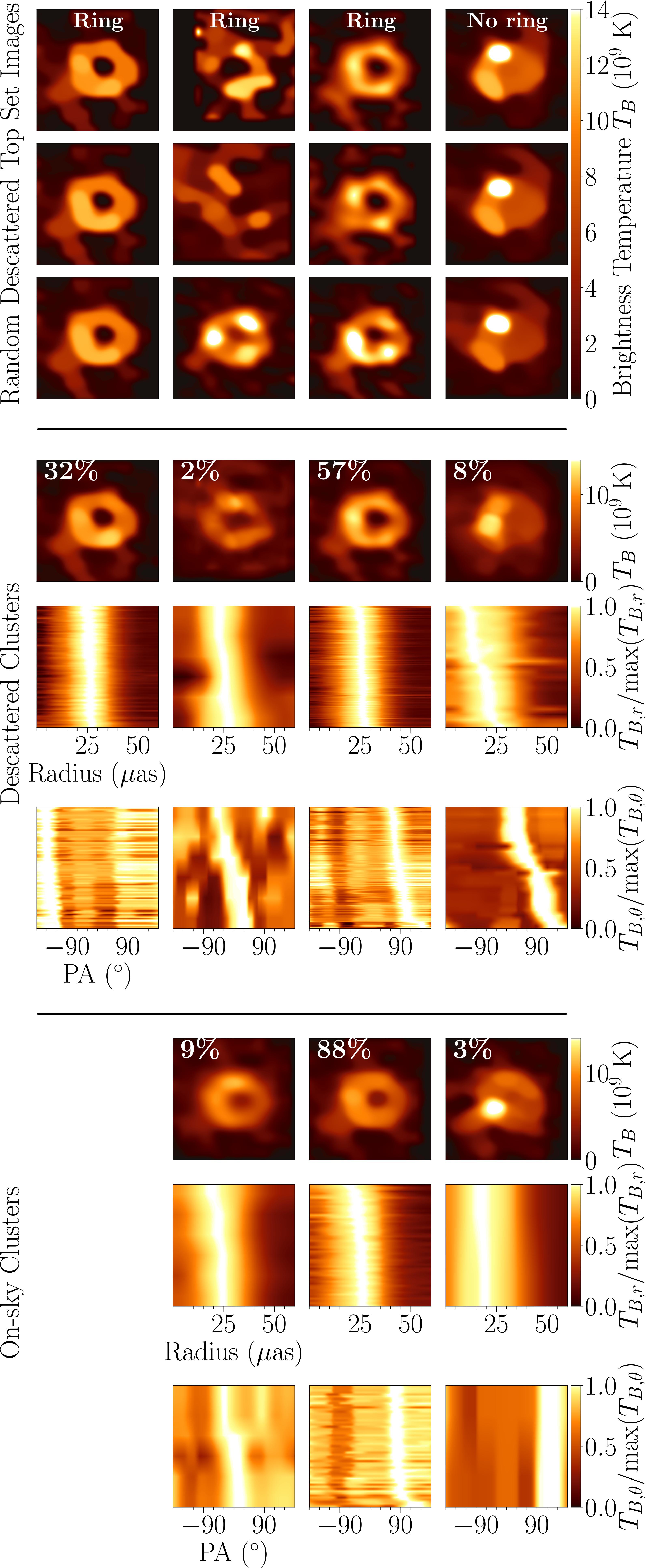
Figure 35: The distribution of Sgr A^∗ Top Set images on April 7 reconstructed with the SMILI dynamic imaging pipeline. We show the distribution of images for each cluster in the same convention with Figure 14 with three horizontal panels separated by horizontal lines. The top panel shows individual images randomly sampled from different clusters. The middle and bottom panels visualize the distributions of reconstructed descattered and on-sky Sgr A^∗ images for each cluster, respectively. In each panel, from top to bottom, we show the average of each cluster, the distributions of the radial profiles, and the distributions of azimuthal intensity profiles.

As described in Section 3.2, the temporal variation of Sgr A^∗ is anticipated to cause significant deviations of visibilities from those of the time-averaged morphology, of which levels can be well characterized by a broken power-law model. As described in Section 7.5.3, the variability noise model allows us to enhance the overall fidelity of synthetic data reconstructions, and enable more sets of the imaging parameter combinations to be selected as Top Sets. However, the prescription for the temporal variability in Section 3.2 include some simplifications of its characteristic properties: for instance, the circular symmetry assumed for the levels of the variability amplitudes in Fourier space and no inclusion of the correlated variations considered in data metrics as covariant components. Here, to assess the dependence of the mitigation scheme for temporal variability, we show the time-averaged images identified by full-track dynamic imaging not relying on the variability noise model. We emphasize that the goal of this section is not to characterize the dynamic evolution of Sgr A^∗ on short timescales, which is the primary focus of Section 9.

As shown in Figure 35, we find the primary three ring morphologies identified in Section 7 with similar azimuthal variations in the most of Top Set images, while non-ring structures are also reconstructed in a small fraction of Top Sets. The results are broadly consistent with those from the imaging survey presented in Section 7, and strongly indicate that our results described in Section 7 are resilient to the methods to recover the time-averaged morphology. We briefly describe the imaging process in Section G.1 and the results in Section G.2.

G.1 SMILI Dynamic Imaging Pipeline and Top Set Selections

Similar to the RML and CLEAN parameter surveys described in Section 6.2, we conducted a large imaging survey with RML dynamic imaging methods (see Section 4.4) implemented in a scripted pipeline using SMILI. The survey was performed on all seven geometric models and Sgr A^∗ data.

After completing the common pre-imaging process of data (Section 6.1), the pipeline reconstructs the time-averaged images on $\sim 8000$ sets of the imaging parameter combinations across a broad parameter space, as outlined in Table 12. With the exactly same criteria described in Section 6.2, Top Sets of the imaging parameters are then selected based on the fidelity of the synthetic data reconstructions.

The SMILI dynamic imaging pipeline shares the same procedures with the SMILI static imaging pipeline described in Section D.3, except for a major difference. Instead of the variability noise model used in Section 6.2, we allow temporal variations on time scales of typical scan intervals — for each set of parameters, the pipeline reconstructs a movie with the frame interval of 1 h, and then time-averages the movie to obtain the resultant reconstruction of the time-averaged morphology. We utilize two temporal regularizers, denoted by $R_{t}$ and $R_{i}$, enforcing the continuity of the frame-to-frame intensity variations and the continuity between each frame and time-averaged intensity distributions, respectively, based on the Euclidian distance between images (see Johnson et al., 2017, for details). We note that here we only explore J18model1 for the scattering mitigation, given consistency among the different scattering mitigation schemes (Section 7.5.2).

G.2 Results

As shown in Figure 35, Top Set images from SMILI dynamic imaging pipeline can be categorized into four clusters shown in Section 7.2. Similar to the RML, CLEAN and Themis static imaging pipelines, the ring morphology with the diameter of $\sim$50 $\mu$as was found as the dominant feature, while the non-ring images were found in a small ($\sim 5$%) fraction of Top Sets. The differences in the image appearance between on-sky and descattered reconstructions are also consistent with Section 7.5.2; the on-sky reconstructions are more blurry than the descattered ones. We note that similar to Top Sets presented in Section 5 and Section 7, here Top Set images from SMILI dynamic imaging pipeline do not constitute a likelihood and therefore the fractions should not represent our degree of certainty.

Appendix H Reconstructions of a Best-bet GRMHD Model in Paper V

In Section 6, we utilize synthetic data based on a GRMHD model selected from a library of time-dependent GRMHD models presented in Paper V (see Section 5.2) to assess the performance of our imaging procedures on a physically motivated evolving source. While this GRMHD model is broadly consistent with our criteria in Section 5 based on 1.3 mm EHT data and light curves, it is not identified as a “best-bet" model in Paper V; “best-bet" models satisfy heterogeneous constraints derived from 1.3 mm EHT data, 86 GHz VLBI observations with the GMVA, 2.2 ${\rm\mu m}$ flux density and x-ray luminosity. Paper V identifies three GRMHD models that lay in a “best-bet” region of strongly magnetized (MAD) models at low inclination with prograde spin.

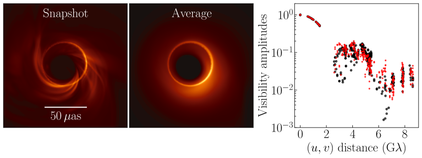
Figure 36: Image and visibility characteristics of the best-bet GRMHD models in Paper V (MAD, $a_{*}=0.5,i=30^{\circ},R_{\rm high}=160$). Left two panels are the snapshot and averaged images of the ground-truth movie. Right panel shows the simulated visibility amplitudes (red) and real Sgr A^∗ measurements (black) as a function of projected baseline length.

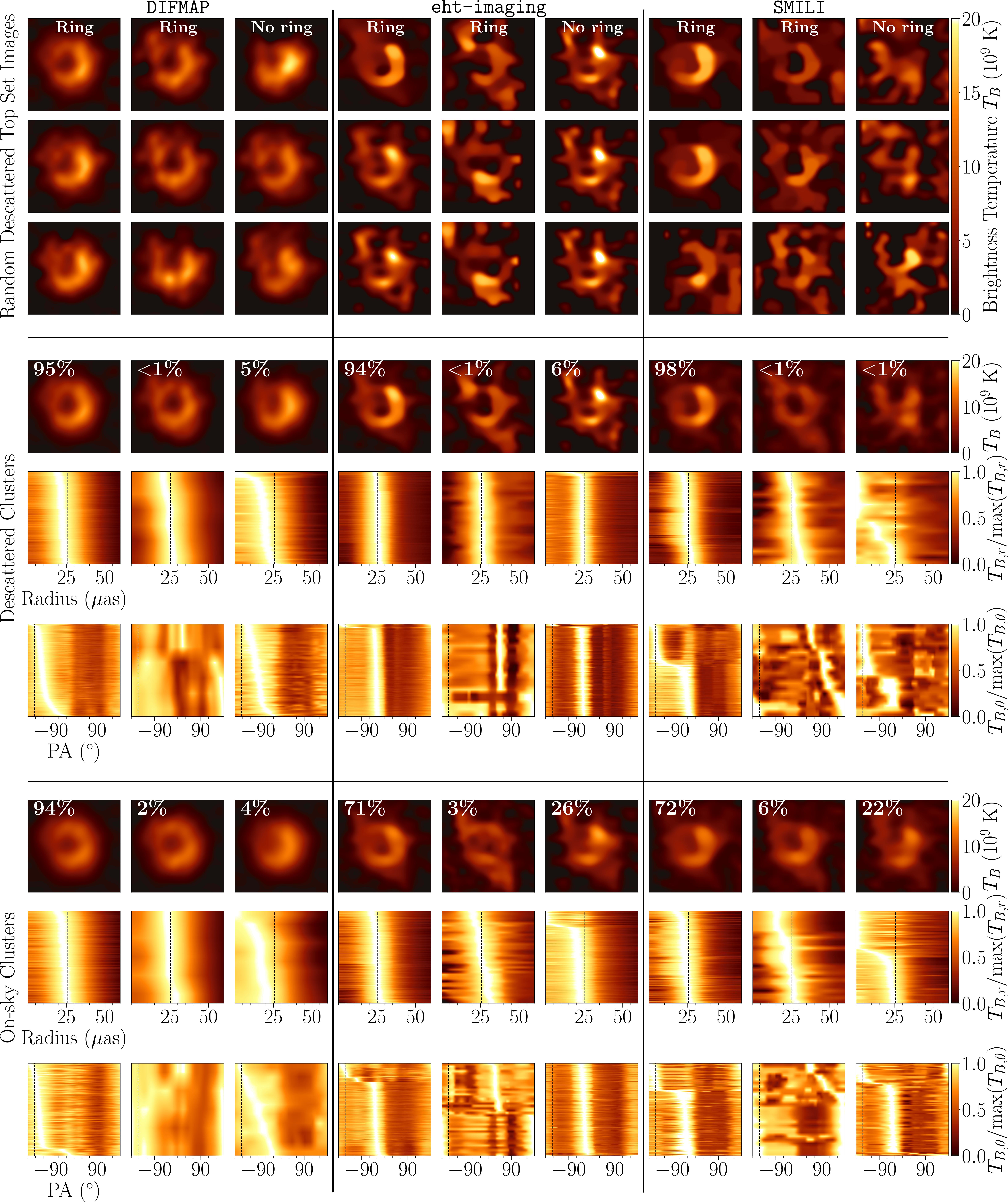
Figure 37: The distribution of reconstructed images with a best-bet GRMHD model identified in paper V. The distribution of images from each pipeline for each cluster is shown with the same convention as Figure 12.

Here we present example reconstructions of synthetic data derived from the “best-bet" model shown in Figure 16 of Paper V, with positive spin of $a_{*}=0.5$ and electron temperature of $R_{\rm high}=160$ viewed at $i=30^{\circ}$. In Figure 36, we show a snapshot and time-averaged images of this GRMHD model, as well as the amplitude versus $(u,v)$-distance corresponding to synthetic data generated with April 7 coverage (generated in the same manner with Section 5). As shown in Figure 36, visibility amplitudes are broadly consistent with EHT Sgr A^∗ data. Figure 37 shows descattered and on-sky images, which are reconstructed with DIFMAP, eht-imaging, and SMILI pipelines using their Top Set parameters and then further categorized by the same clustering method presented in Appendix F.

As shown in Figure 37, the distributions of the Top Set images share key results from those of the GRMHD reconstructions described in Section 6.4.2 (see also Figure 12). The vast majority of the reconstructions identify a ring morphology with a diameter of $\sim$50 $\mu$as, consistent with the ground-truth model. However, a small fraction of images have a non-ring morphology. Furthermore, ring reconstructions have multiple azimuthal intensity modes. In particular, ring images that have a peak PA of $\sim-154^{\circ}$ consistent with the ground-truth image do not appear as the most popular modes in eht-imaging and SMILI reconstructions. The broad consistency with the results in Section 6.4.2 suggest that our main results (e.g., that for the RML and CLEAN pipelines our methods produce a small fraction of non-ring modes for an underlying ring model, and that the most popular mode reconstructed is not always that true mode) likely generalize across GRMHD models that are in a broad agreement with 1.3 mm EHT data.

Appendix I Ring fitting parameters

In Table 13 and Table 14 we list the diameter $d$, width $w$, position angle $\eta$, asymmetry $A$, and fractional central brightness $f_{c}$ measured from Top Set Sgr A^∗ images for each identified cluster (see Section 8) corresponding to the descattered and on-sky images, respectively.

Table 13: Mean and standard deviation of ring parameters, diameter $d$, width $w$, position angle $\eta$, asymmetry $A$, and fractional central brightness $f_{c}$ measured from Top Set or posterior descattered Sgr A^∗ images for each cluster.

		$d\ \rm{(\mu as)}$	$w\ \rm{(\mu as)}$	$\eta\ \rm{(^{\circ})}$	$A$	$f_{c}$
DIFMAP
April 6 Ring	REx	$46\pm 4.1$	$33\pm 3.5$	$-100.6\pm 73.4$	$0.15\pm 0.08$	$0.47\pm 0.14$
	VIDA	$51\pm 3.1$	$33\pm 3.1$	$-108.3\pm 79.2$	$0.26\pm 0.12$	$0.46\pm 0.11$
April 7 Ring 1		$50\pm 1.9$	$31\pm 2.7$	$-92.0\pm 42.0$	$0.06\pm 0.04$	$0.40\pm 0.08$
		$51\pm 1.3$	$33\pm 1.4$	$-82.7\pm 40.5$	$0.07\pm 0.07$	$0.37\pm 0.08$
April 7 Ring 2		$49\pm 3.2$	$32\pm 2.9$	$-22.5\pm 54.4$	$0.08\pm 0.06$	$0.45\pm 0.12$
		$50\pm 1.7$	$32\pm 1.4$	$-27.0\pm 47.4$	$0.12\pm 0.11$	$0.42\pm 0.11$
April 7 Ring 3		$49\pm 1.8$	$32\pm 2.9$	$20.5\pm 47.2$	$0.08\pm 0.05$	$0.44\pm 0.09$
		$51\pm 1.6$	$33\pm 1.8$	$5.3\pm 38.9$	$0.12\pm 0.10$	$0.41\pm 0.10$
eht-imaging
April 6 Ring	REx	$56\pm 4.5$	$24\pm 2.4$	$32.3\pm 86.4$	$0.17\pm 0.05$	$0.16\pm 0.14$
	VIDA	$59\pm 11.3$	$30\pm 10.4$	$70.0\pm 88.3$	$0.24\pm 0.14$	$0.23\pm 0.19$
April 7 Ring 1		$55\pm 1.9$	$26\pm 2.3$	$-140.6\pm 62.9$	$0.11\pm 0.04$	$0.18\pm 0.08$
		$56\pm 5.4$	$27\pm 2.5$	$-156.0\pm 60.6$	$0.15\pm 0.13$	$0.18\pm 0.09$
April 7 Ring 2		$53\pm 1.8$	$27\pm 2.7$	$-60.1\pm 35.8$	$0.12\pm 0.05$	$0.23\pm 0.10$
		$53\pm 3.6$	$27\pm 4.0$	$-71.7\pm 33.1$	$0.15\pm 0.11$	$0.22\pm 0.10$
April 7 Ring 3		$55\pm 1.5$	$27\pm 3.0$	$170.4\pm 101.4$	$0.12\pm 0.07$	$0.31\pm 0.17$
		$57\pm 6.4$	$26\pm 4.5$	$179.7\pm 67.1$	$0.18\pm 0.21$	$0.27\pm 0.11$
SMILI
April 6 Ring	REx	$57\pm 3.4$	$24\pm 1.9$	$-27.7\pm 43.8$	$0.23\pm 0.09$	$0.03\pm 0.10$
	VIDA	$46\pm 12.0$	$50\pm 16.6$	$-71.6\pm 123.8$	$0.18\pm 0.12$	$0.59\pm 0.33$
April 7 Ring 1		$52\pm 5.0$	$26\pm 2.0$	$151.9\pm 75.8$	$0.12\pm 0.04$	$0.22\pm 0.10$
		$52\pm 3.8$	$27\pm 3.9$	$175.9\pm 77.6$	$0.10\pm 0.08$	$0.22\pm 0.09$
April 7 Ring 2		$53\pm 4.0$	$25\pm 2.9$	$-39.3\pm 51.2$	$0.13\pm 0.06$	$0.23\pm 0.11$
		$52\pm 6.2$	$29\pm 8.4$	$-59.2\pm 64.9$	$0.15\pm 0.12$	$0.27\pm 0.18$
April 7 Ring 3		$51\pm 4.0$	$26\pm 1.9$	$109.1\pm 55.2$	$0.13\pm 0.04$	$0.19\pm 0.09$
		$51\pm 3.0$	$27\pm 3.8$	$116.2\pm 65.0$	$0.10\pm 0.08$	$0.19\pm 0.08$
Themis
April 6 Ring	REx	$51\pm 3.9$	$25\pm 1.2$	$-128.6\pm 10.0$	$0.20\pm 0.04$	$0.27\pm 0.10$
	VIDA	$54\pm 0.9$	$24\pm 0.9$	$-121.0\pm 21.7$	$0.27\pm 0.06$	$0.34\pm 0.08$
April 7 Ring 1		$53\pm 0.5$	$23\pm 1.4$	$-37.5\pm 11.3$	$0.14\pm 0.01$	$0.09\pm 0.07$
		$56\pm 1.4$	$27\pm 0.9$	$-37.6\pm 7.6$	$0.30\pm 0.05$	$0.19\pm 0.07$
April 7 Ring 2		$53\pm 0.7$	$22\pm 0.5$	$-12.5\pm 8.3$	$0.21\pm 0.02$	$0.05\pm 0.05$
		$56\pm 1.2$	$27\pm 0.7$	$-20.6\pm 6.1$	$0.36\pm 0.04$	$0.15\pm 0.03$
April 7 Ring 3		-	-	-	-	-
		-	-	-	-	-

Table 14: Mean and standard deviation of ring parameters, diameter $d$, width $w$, position angle $\eta$, asymmetry $A$, and fractional central brightness $f_{c}$ measured from Top Set and posterior on-sky Sgr A^∗ images for each cluster.

		$d\ \rm{(\mu as)}$	$w\ \rm{(\mu as)}$	$\eta\ \rm{(^{\circ})}$	$A$	$f_{c}$
DIFMAP
April 6 Ring	REx	$46\pm 3.0$	$34\pm 4.3$	$97.9\pm 88.9$	$0.11\pm 0.05$	$0.50\pm 0.15$
	VIDA	$47\pm 1.9$	$39\pm 3.4$	$94.8\pm 87.0$	$0.14\pm 0.07$	$0.56\pm 0.10$
April 7 Ring 1		$47\pm 3.0$	$38\pm 2.7$	$-111.6\pm 39.7$	$0.06\pm 0.03$	$0.59\pm 0.07$
		$49\pm 2.2$	$37\pm 1.9$	$-99.9\pm 40.2$	$0.09\pm 0.06$	$0.58\pm 0.08$
April 7 Ring 2		$48\pm 2.4$	$38\pm 2.6$	$31.3\pm 81.2$	$0.06\pm 0.04$	$0.58\pm 0.07$
		$49\pm 2.0$	$37\pm 2.1$	$16.0\pm 75.7$	$0.10\pm 0.06$	$0.56\pm 0.07$
April 7 Ring 3		$48\pm 2.7$	$37\pm 2.9$	$40.4\pm 63.5$	$0.05\pm 0.03$	$0.57\pm 0.08$
		$50\pm 2.1$	$38\pm 1.9$	$27.6\pm 60.9$	$0.08\pm 0.06$	$0.55\pm 0.08$
eht-imaging
April 6 Ring	REx	$49\pm 3.9$	$28\pm 3.6$	$13.8\pm 123.8$	$0.15\pm 0.05$	$0.33\pm 0.15$
	VIDA	$50\pm 5.6$	$41\pm 6.7$	$110.8\pm 133.2$	$0.20\pm 0.10$	$0.55\pm 0.13$
April 7 Ring 1		$51\pm 2.4$	$32\pm 2.7$	$-165.9\pm 45.0$	$0.08\pm 0.03$	$0.42\pm 0.10$
		$52\pm 4.5$	$35\pm 3.5$	$-170.7\pm 41.1$	$0.11\pm 0.10$	$0.41\pm 0.08$
April 7 Ring 2		$50\pm 2.3$	$32\pm 2.7$	$-30.4\pm 68.1$	$0.07\pm 0.03$	$0.44\pm 0.07$
		$49\pm 2.6$	$35\pm 4.0$	$-71.6\pm 53.5$	$0.06\pm 0.08$	$0.42\pm 0.08$
April 7 Ring 3		$49\pm 2.4$	$33\pm 3.3$	$161.6\pm 67.3$	$0.10\pm 0.02$	$0.50\pm 0.08$
		$53\pm 6.6$	$35\pm 7.5$	$173.3\pm 70.8$	$0.19\pm 0.14$	$0.52\pm 0.10$
SMILI
April 6 Ring	REx	$43\pm 0.4$	$28\pm 3.1$	$163.1\pm 10.1$	$0.10\pm 0.04$	$0.57\pm 0.01$
	VIDA	$39\pm 3.9$	$46\pm 8.8$	$-98.6\pm 93.3$	$0.17\pm 0.14$	$0.67\pm 0.16$
April 7 Ring 1		$43\pm 4.9$	$33\pm 1.7$	$127.7\pm 29.9$	$0.09\pm 0.08$	$0.51\pm 0.07$
		$45\pm 1.8$	$34\pm 3.1$	$136.8\pm 36.8$	$0.07\pm 0.06$	$0.48\pm 0.07$
April 7 Ring 2		$47\pm 4.5$	$33\pm 2.8$	$58.4\pm 57.5$	$0.10\pm 0.05$	$0.48\pm 0.11$
		$46\pm 5.2$	$37\pm 7.4$	$59.8\pm 81.7$	$0.08\pm 0.08$	$0.50\pm 0.13$
April 7 Ring 3		$48\pm 4.3$	$32\pm 2.9$	$89.6\pm 34.9$	$0.11\pm 0.04$	$0.45\pm 0.14$
		$47\pm 3.5$	$35\pm 4.3$	$84.8\pm 48.2$	$0.11\pm 0.08$	$0.46\pm 0.11$
Themis
April 6 Ring	REx	$46\pm 2.1$	$30\pm 1.6$	$-139.4\pm 52.9$	$0.15\pm 0.05$	$0.34\pm 0.11$
	VIDA	$47\pm 3.1$	$33\pm 2.0$	$-127.4\pm 53.0$	$0.17\pm 0.08$	$0.42\pm 0.07$
April 7 Ring 1		$51\pm 0.8$	$28\pm 1.3$	$-37.8\pm 53.6$	$0.15\pm 0.01$	$0.21\pm 0.10$
		$55\pm 1.6$	$32\pm 2.4$	$-41.4\pm 52.6$	$0.25\pm 0.05$	$0.30\pm 0.07$
April 7 Ring 2		$50\pm 1.5$	$26\pm 1.1$	$-16.0\pm 8.9$	$0.21\pm 0.03$	$0.20\pm 0.08$
		$56\pm 2.6$	$32\pm 0.9$	$-25.2\pm 7.3$	$0.35\pm 0.03$	$0.29\pm 0.06$
April 7 Ring 3		-	-	-	-	-
		-	-	-	-	-

Appendix J Dynamic Imaging and Snapshot Model Fitting tests

J.1 Selection of Time Windows with the Best $(u,v)$-coverage

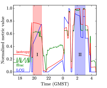
Figure 38: Normalized metric computations for every scan of the April 7, 2017 EHT coverage of Sgr A^∗. 0:00 GMST marks the day change from April 7 to April 8. Though the metrics have different considerations, all highlight the region (labelled “II”) from ${\sim}$1:30 GMST to ${\sim}$3:10 GMST as a candidate region for dynamic imaging.

Farah et al. (2021) demonstrates that the changing $(u,v)$-coverage created by the Earth’s rotation during the aperture synthesis process leads to regions of time that produce dynamic reconstructions of varying quality. The quality of a short-timescale reconstruction is partially determined by the snapshot $(u,v)$-coverage geometry, which introduces certain artifacts during the imaging process.

The scale and severity of these artifacts can be predicted by quantitatively scoring the $(u,v)$-coverage as a function of time, which can be done in a number of ways. Some metrics examine how much of the Fourier plane is covered by an interferometer (e.g., Palumbo et al. 2019), while others look at gaps created by the sparse coverage (e.g., Wielgus et al. 2020). In addition to these metrics, Farah et al. (2021) derives a novel metric that probes both the anisotropy and radial homogeneity of the coverage.

By applying these metrics to the April 6 and 7 EHT $(u,v)$-coverage on Sgr A^∗, we can assess the scan-by-scan performance and identify regions of time which are likely to produce the best reconstructions, independent of the underlying source structure. The result of such an analysis for April 7 is shown in Figure 38, and two candidate regions are highlighted. The metrics predict dynamic imaging reconstructions will have the highest quality in the region from 1.5-3.2 GMST (Region II); the reconstructions will produce substantially worse results in the region from 19.4-21 GMST (Region I). We validate this prediction by testing on high S/N data in Farah et al. (2021) and show that Region II indeed allows for significantly better recovery of the source variability than Region I. Therefore, based only on the EHT’s $(u,v)$-coverage, we focus on dynamic imaging/modeling Region II throughout Section 9.

J.2 Starwarps Temporal Regularizer Normalization

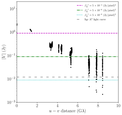
Figure 39: April 7 EHT visibility amplitudes over the selected window for dynamic imaging and modeling (black points). The horizontal lines show the expected standard deviation of the visibility amplitudes in StarWarps reconstructions for different values of $\beta^{-1}_{Q}$ in units of $(\text{Jy/pixel})^{2}$: $5\times 10^{-4}$ (magenta), $5\times 10^{-6}$ (green), and $5\times 10^{-8}$ (cyan).

Temporal regularization in StarWarps is controlled by a parameter $\beta_{Q}^{-1}$. This parameter corresponds to the variance of the conditional distribution of pixel intensities for a given snapshot holding the previous snapshot fixed: $p(I_{k}|I_{k-1})=\mathcal{N}(I_{k-1},\beta^{-1}_{Q}\mathbbm{1})$. The units of $\beta_{Q}^{-1}$ are $(\text{Jy/pixel})^{2}$. In the main text, we consider values $\beta^{-1}_{Q}\in\{5\times 10^{-4},5\times 10^{-6},5\times 10^{-8}\}$. Larger values of $\beta^{-1}_{Q}$ correspond to less temporal regularization, as the conditional distribution $p(I_{k}|I_{k-1})$ becomes wider.

We can also interpret the values $\beta^{-1}_{Q}$ in visibility space. The Fourier transform of the image $I_{k}$ is given by a $N_{\rm pix}\times N_{\rm pix}$ matrix $\mathbf{F}$:

$$V_{k}=\mathbf{F}I_{k}.$$ (J1)

In our convention, the pixel values in $I_{k}$ have units Jy/pixel, so the entries of $\mathbf{F}$ are pure phase terms without a $1/\sqrt{N}$ normalization (so that, for instance, the zero-baseline visibility in Jy is just the sum of the pixel intensities). As a result $\mathbf{F}\mathbf{F}^{\dagger}=N_{\rm pix}\mathbbm{1}$. Because Equation J1 is a linear transformation, $p(V_{k}|I_{k-1})$ is also a normal distribution, with a mean $V_{k-1}$ and a covariance:

$$\mathbf{\Sigma}=\mathbf{F}\left[\beta^{-1}_{Q}\mathbbm{1}\right]\mathbf{F}^{\dagger}=\beta^{-1}_{Q}N_{\rm pix}\mathbbm{1}.$$ (J2)

Thus, $\sigma_{\rm vis}\equiv\sqrt{\beta^{-1}_{Q}N_{\rm pix}}$ is the standard deviation of a snapshot visibility measurement in StarWarps, holding the previous frame fixed.

In Figure 39, we compare this quantity to the measured EHT visibility amplitudes in the selected dynamic imaging window on April 11. The StarWarps movie reconstructions in the main text have $N_{\rm pix}=40\times 40=1600$. GRMHD simulations (see Paper IV and Georgiev et al. 2021) and the light curve of Sgr A^∗ (see Wielgus et al., 2022) suggest that the variations on minute timescales should have a zero-baseline standard deviation of $\sigma_{\rm vis}\sim 10\,{\rm mJy}$. Thus, reconstructions with $\beta^{-1}_{Q}\sim 10^{-7}({\rm Jy/pixel})^{2}$ are expected to give variability that is consistent with what is measured in Sgr A^∗.

Larger values of $\beta^{-1}_{Q}$ correspond to lower temporal regularization and allow for larger variations in the visibility amplitudes. For instance, our reconstructions in Section 9 with $\beta^{-1}_{Q}=5\times 10^{-6}$ permit somewhat more variability than is seen in simulations and observations of Sgr A^∗. Nevertheless, we have also found that allowing excess variability helps to trace evolution in tests on synthetic data from GRMHD simulations.

J.3 Testing $(u,v)$-coverage Effects

As discussed in Section 9.2, the geometry of the $(u,v)$-coverage can have an effect on the recovered image structure, especially in cases where the coverage is extremely sparse. To study the effects of $(u,v)$-coverage on dynamic fits to Sgr A^∗ data, we perform a number of tests on synthetic data sets and study the effect of different $(u,v)$ baselines on fits to the real data.

J.3.1 Recovering the Position Angle of a Static Crescent

As most of our analysis of the dynamic structure of Sgr A^∗ revolves around tracking the position angle (PA) of brightness around the ring, it is important to assess our ability to recover the PA accurately in realistic synthetic data. To that end, we constructed synthetic EHT data sets from 4 static crescent models with peak brightness points rotated at 60^∘ increments around the ring. The brightness ratio of each crescent model was chosen to roughly match the 1.5:1 ratio recovered from geometric model fitting to Sgr A^∗ data. Figure 40 shows the imaging and geometric modeling results obtained by fitting to these synthetic data sets in the selected 1.7 h region. Note that, for both approaches, the true PA is recovered as the primary mode for most of the crescents. The imaging methods contain temporal regularization, which likely makes it easier to recover a static underlying structure; however, the geometric modeling results do not assume any temporal regularization.

J.3.2 Uniform Ring Synthetic Data

The interplay between the source size and sidelobes in the dirty beam pattern from sparse coverage can cause imaging artifacts that appear in the form of bright “knots" around ring sources. Computing the dirty image of an underlying uniform ring source reveals the location of these knots when using calibrated visibilities. To assess the impact of these knot artifacts on our analysis we performed imaging and geometric model fitting on data generated from a uniform ring (with no brightness changes in azimuth) with diameter of 49 $\mu$as (refer to the uniform ring in Figure 7). As can be seen in Figure 40, both the imaging and modeling results indicate an image structure with a preferred PA – $\sim 0^{\circ}$ or $\sim 90^{\circ}$ for imaging and $\sim 100^{\circ}$ for modeling. However, the associated asymmetry of the recovered uniform ring is very low, a brightness ratio of less than 1.1:1 compared to 1.5:1 for Sgr A^∗. Thus, in combination with the results of Section J.3.1, we conclude that although the $(u,v)$-coverage will bias the PA in the limit of low image asymmetry, for the level of image asymmetry recovered in Sgr A^∗ this bias should have a small effect.

J.3.3 Baseline Test

In order to evaluate the contribution of each baseline to the recovered evolution in Sgr A^∗, we compared results obtained on data sets modified to remove a particular baseline. In particular, we compared the PA posteriors obtained using geometric modeling on 11 different data sets – 10 data set each with a single baselines removed and one complete data set. As can be seen in Figure 41, we find that most baselines do not heavily affect the trends we see on April 7. However, there are two baselines that appear to have a significant effect on the results: Chile–Hawaiʻi and LMT–Hawaiʻi. Without the Chile–Hawaiʻi baseline we are not able to discriminate between the northwest and southeast PA; without the LMT–Hawaiʻi baseline we do not recover as significant of a PA shift. Upon inspecting the $(u,v)$-coverage of these baselines it becomes apparent that these two baselines probe the northwest to southeast orientations that we are interested in, and thus without them we are unable to properly discriminate between these two PA orientations. It is also worth noting that removal of the Chile-SPT baseline appears to “clean up" the modeling results, suggesting that small-scale features probed by this baseline may not be properly captured in our geometric model fits.

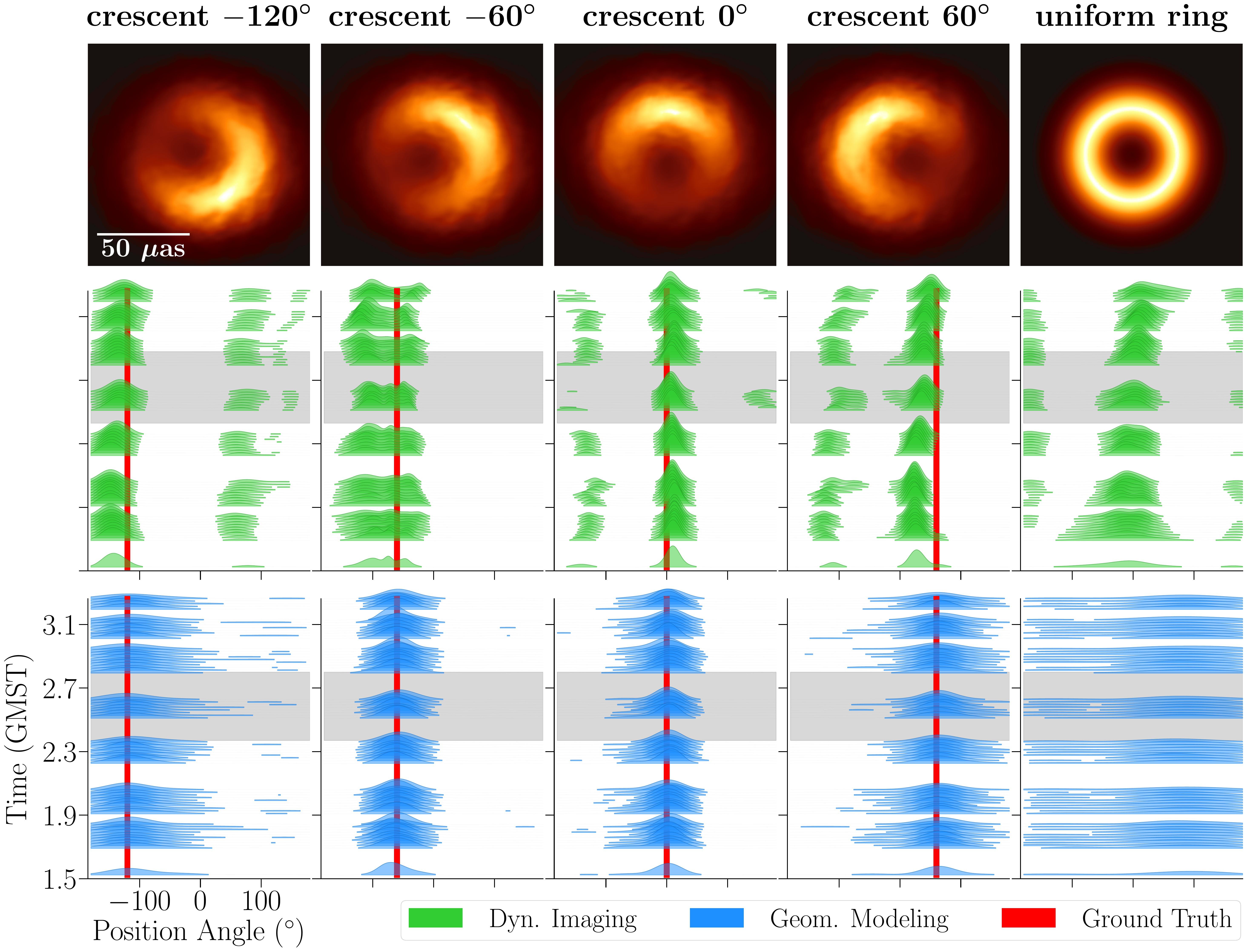
Figure 40: Position angle (PA) recovered from differently oriented static crescents synthetic data sets and a uniform ring synthetic data set, using both dynamic imaging (green) and geometric modeling (blue) techniques. The crescents’ ground truth PA is shown as a vertical red line. Imaging uses a prior image $\mu$ of a uniform ring convolved with a 25 $\mu$as beam.

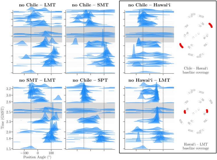
Figure 41: Position angle (PA) recovered using DPI geometric modeling after removal of a particular baseline from Sgr A^∗ data on April 7. The flagged baseline appears in the title of each panel. The Chile-Hawaiʻi and Hawaiʻi-LMT baselines are highlighted and their location in the $(u,v)$ plane is shown. These two baselines probe the east–west and southeast–northwest orientations.

J.4 Testing Scattering Mitigation Strategies

In producing dynamic reconstructions and model fits of the Sgr A^∗ data, the choice of scattering mitigation strategy is a potential source of uncertainty. We have explored the sensitivity of our dynamic imaging and snapshot model fitting results to the same five scattering mitigation strategies we consider in the static image surveys in Section 6 and Section 7.5.2. Namely, we produce reconstructions and model fits to the unmodified data (i.e., on-sky with no descattering), as well as with visibilities deblurred by the Sgr A^∗ diffractive scattering kernel and with the thermal noise error bars inflated by four models of the refractive noise: the Const model, the J18model1 model, and then double the additional error tolerance from each of these models (2$\times$Const, 2$\times$J18model1). Based on the analysis done in Section 3.1, this selection is conservative and spans our uncertainty in Sgr A^∗’s refractive noise.

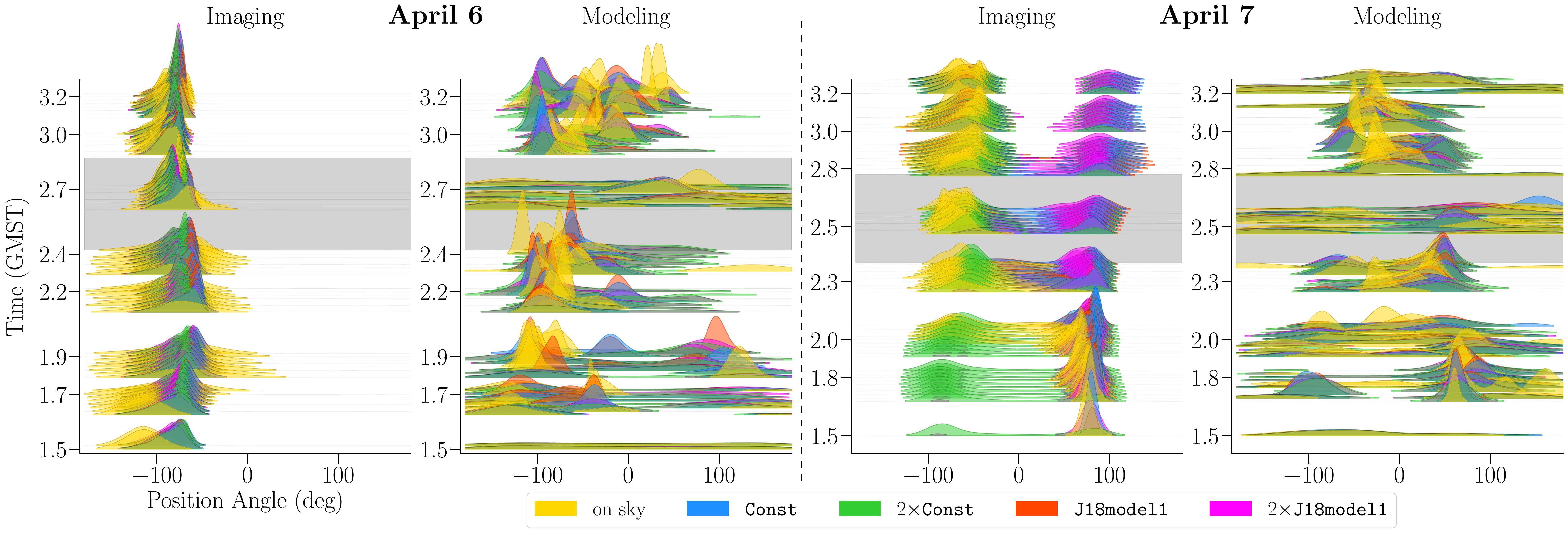
Figure 42: The position angle (PA) recovered using dynamic imaging and geometric modeling techniques under different scattering mitigation assumptions. These range from no scattering mitigation whatsoever (yellow), to different amounts of refractive noise added to the deblurred data: a constant noise floor (blue), the refractive noise model J18model1 (red), and these two scaled by a factor of two (green and magenta, respectively). Imaging results were obtained using an initialization/prior image of a uniform ring blurred with a Gaussian kernel with FWHM of 25 $\mu$as. Modeling results were obtained from the DPI pipeline using the $m$-ring 2 geometric model. The gray band at roughly 2.6 GMST indicates the region where the LMT has dropped out and data coverage is poorer.

Figure 42 presents comparisons of the StarWarps reconstructions and snapshot model fitting results on the April 6 and 7 Sgr A^∗ data with all five scattering mitigation strategies. We find that the general trends in the ring position angle we discuss in Section 9.4 are not significantly changed by any of the five scattering mitigation strategies we explore for geometric modeling, although the position angle posteriors are significantly broader (sometimes spanning a full 360^∘) when using the larger refractive noise budgets of 2$\times$Const and 2$\times$J18model1. In contrast, for imaging, on April 7, we observe a transition from positive to negative PA to be the most commonly recovered trend with all of the on-sky, Const and J18model1 scattering mitigation strategies when using a ring prior. However, when we add a very large amount of refractive noise tolerance to the error bars in the 2$\times$Const and 2$\times$J18model1 models, the PA becomes more stable over the observation window. This is due to the interplay of temporal regularization with an increased flexibility in fitting the data with a static model due to the expanded noise budget. In this figure, imaging with StarWarps makes use of the ring$\textasteriskcentered$25$\mu$as ring prior/initialization and modeling with DPI uses a second order $m$-ring ($m=2$) model with a parameterized central Gaussian floor.

J.5 Testing the Effects of Different Imaging Priors and Model Specifications

As overviewed in Section 9.4.1, the recovered PA of the azimuthal brightness distribution in the ring-like morphology of Sgr A^∗ is sensitive to the modeling choices made in both imaging and geometric modeling. In this section we go into further detail on some of the effects seen.

J.5.1 Imaging

Temporal regularization

The level of continuity enforced between recovered frames is controlled by temporal regularization. In particular, StarWarps encourages frames to be similar by probabilistically modeling each frame $I_{k}$ as being a sample from a normal distribution with mean $I_{k-1}$ and covariance $\beta_{Q}^{-1}\mathbbm{1}$ (see Equation 7). Thus, decreasing the multiplier $\beta_{Q}^{-1}$ will increase recovered continuity between frames. This is seen, as expected, in the recovered movies of Sgr A^∗ visualized in Figure 28; recovered movies with low temporal regularization experience fast and drastic variability on large scale features, while movies with high temporal regularization experience slow yet steady variability on large-scale features and absorb the remaining variability in the data with small scale fluctuations. Due to the extreme sparsity of data on each snapshot, although these movies contain significantly different levels of recovered variability, they all fit the data in terms of $\chi^{2}$ fairly well. The only substantial difference between data fits can be seen when inspecting the SMT-LMT-Hawaiʻi closure triangle. It is worth noting that the positive to negative flip on the April 7’s closure triangle is not reproduced by the recovered video with high temporal regularization. Nonetheless, since all movies still match all remaining baselines indistinguishably well it is difficult to form any solid conclusions on the type of variability in Sgr A^∗ based on this one closure triangle.

StarWarps spatial prior images

To explore the sensitivity of results to the ring features encouraged during imaging, we introduce 5 different images used as both the initialization and mean prior image $\mu$ in StarWarps. Figure 43 shows the mean prior images explored for imaging the original data and deblurred data. Note that recovered flux is constrained to evolve within the regions that have flux in the prior image, therefore the puffier rings and the tapered disk with more extended flux are less constraining during imaging. As expected, movies recovered with the less constraining puffier prior images result in recovered movies with a less clear underlying ring structures. Nonetheless, in all these cases (with a ring init/prior), the same general trend in PA is recovered in one of the modes, even when the central indent is very weak. When a disk prior is used with no central indent whatsoever the same PA trend is not recovered; instead, the PA trend appears to be reversed in sign (as discussed in Figure 27). Figure 44 shows more detailed comparisons of StarWarps movies reconstructed with ring and disk mean prior images on April 6 and 7, including data fits to representative closure phases.

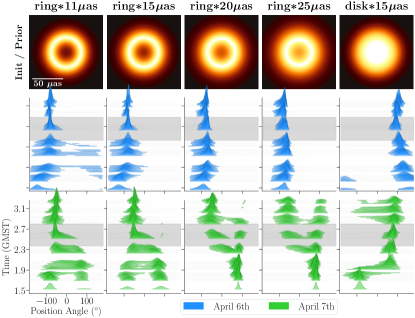
Figure 43: Position angle (PA) reconstructed using StarWarps under different init/prior assumptions for both April 6 (blue) and 7 (green). These include uniform rings with increasing Gaussian blurring and a uniform disk with no central brightness depression.

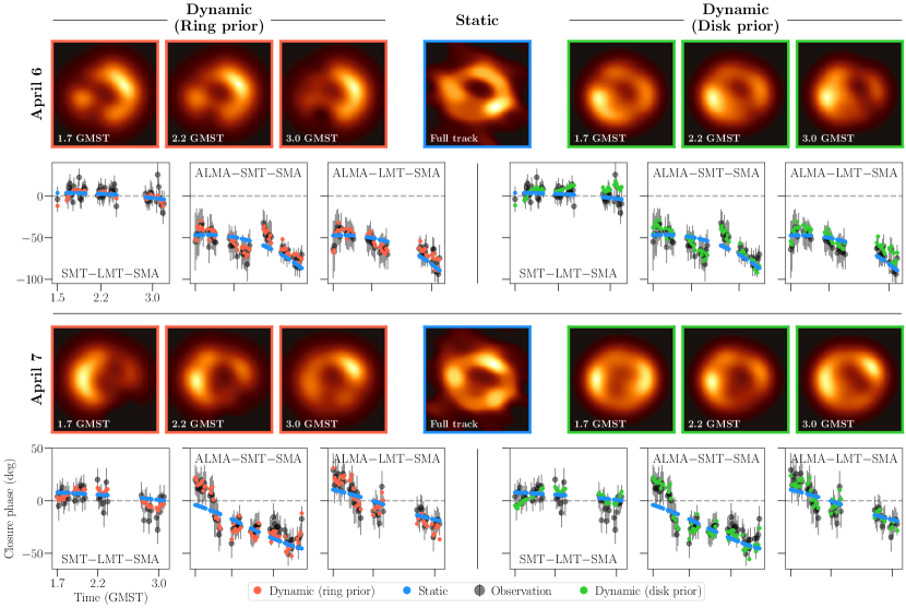
Figure 44: Comparing data fit of descattered dynamic imaging versus static imaging on April 7. A representative descattered image from the eht-imaging static imaging pipeline is shown. In the selected closure plots below the measured data (60 s avg. without a variability noise budget) is shown overlaid with the corresponding closure phases.

J.5.2 Geometric Modeling

For snapshot geometric modeling, we have two competing effects. One is that we require a geometric model that can adequately explain the on-sky image. However, given the sparseness of the $(u,v)$-coverage for each snapshot, the risk of over-fitting the data is considerable and potentially leads to artificially un-informative posteriors. However, under-fitting the data can lead to large biases in the recovered parameters, and artificially narrow posteriors. To find the preferred model we use relative measures. That is, we don’t compare the absolute fit quality using a metric like the $\chi^{2}$ statistic, but rather how well a model does compared to the others considered. For this purpose we use the Bayesian evidence (also referred to as evidence),

$$Z({\rm data}|M)=\int\mathcal{L}({\rm data}|\theta,M)p(\theta|M)\mathrm{d}\theta.$$ (J3)

The evidence measures the marginal probability of the data, after averaging over all possible parameter values of the model. The preferred model is then the one that maximizes the evidence of the model. For snapshot modeling we select the preferred model by computing the log-evidence in each snapshot, and then sum the log-evidence across all snapshots. Note, that we are only able to estimate the evidence for the Comrade pipeline. DPI/Variational inference cannot estimate the evidence, but instead can compute an effective lower bound to use as a proxy.

M-ring Order

To assess the impact of different model choices on the posterior samples, we considered an $m$-ring model with 1–4 modes. The results for the $m$-ring model from the Comrade pipeline are shown in Figure 45. We find that the trend for the dipole moment phase is consistent across model specifications, albeit the posteriors become more uncertain for the higher-order $m$-ring models. The recovered total evidence for each model is shown in Figure 45. For April 6 $m=4$ is the preferred model with a log-evidence of $1499$. On April 7, the $m=2$ $m$-ring is preferred with a log-evidence of $1667$. On both days the overall trend of the position angle maintains stable for $m=1,2,3$, but the distributions become noticeably wider.

For the DPI pipeline we find similar PA trends for April 6 and 7. Using the evidence-lower-bound (ELBO) that is calculated as part of variational methods, $m=3$ being preferred on April $6$ and $m=1$ on April 7. Furthermore, on April 7 the PA posterior for $m=3,4$ is very broad, becoming essentially unconstrained.

Comparing the DPI results to Comrade we find that $m=1$ is preferred on April 7 and $m=3$ on April 6 according to the evidence lower bound. DPI fits closure products which are equivalent to placing uniform priors on gains, meaning that the data is less constraining. Therefore, it is not surprising that DPI prefers simpler models compared to Comrade. To select a fiducial model across days and bands we considered both the evidence, the relative impact on the posterior, and impact on each pipeline. For these reasons we take $m=2$ for DPI and $m=2$ and sometimes $m=3$ for Comrade. The $m=2$ model is preferred for Comrade on April 7 and the $m=2$ distribution for DPI is similar but broader than the $m=1$.

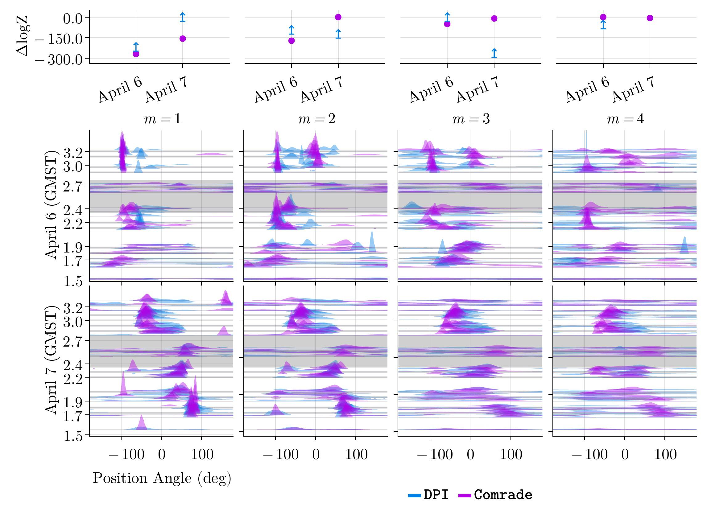
Figure 45: Comparing the $m$-ring results across orders 1, 2, 3, and 4 in both Comrade (magenta) and DPI (blue). The impact of the different $m$-ring orders on the position angle evolution for April 6 and 7 are shown in the middle and bottom rows. The top row is the change in the log-evidence across $m$-ring orders and days. The evidence lower bound produced by DPI is shown as a blue upwards arrow.

References

- Akiyama et al. (2013) Akiyama, K., Takahashi, R., Honma, M., Oyama, T., & Kobayashi, H. 2013, PASJ, 65, 91
- Akiyama et al. (2017a) Akiyama, K., Kuramochi, K., Ikeda, S., et al. 2017a, ApJ, 838, 1
- Akiyama et al. (2017b) Akiyama, K., Ikeda, S., Pleau, M., et al. 2017b, AJ, 153, 159
- Alberdi et al. (1993) Alberdi, A., Lara, L., Marcaide, J. M., et al. 1993, A&A, 277, L1
- Arras et al. (2019) Arras, P., Frank, P., Leike, R., Westermann, R., & Enßlin, T. A. 2019, A&A, 627, A134
- Astropy Collaboration et al. (2013) Astropy Collaboration, Robitaille, T. P., Tollerud, E. J., et al. 2013, A&A, 558, A33
- Astropy Collaboration et al. (2018) Astropy Collaboration, Price-Whelan, A. M., Sipőcz, B. M., et al. 2018, AJ, 156, 123
- Baganoff et al. (2003) Baganoff, F. K., Maeda, Y., Morris, M., et al. 2003, ApJ, 591, 891
- Balick & Brown (1974) Balick, B., & Brown, R. L. 1974, ApJ, 194, 265
- Bardeen (1973) Bardeen, J. M. 1973, Les Astres Occlus, 215
- Blackburn et al. (2020) Blackburn, L., Pesce, D. W., Johnson, M. D., et al. 2020, ApJ, 894, 31
- Blackburn et al. (2019) Blackburn, L., Chan, C.-k., Crew, G. B., et al. 2019, ApJ, 882, 23
- Bouman (2017) Bouman, K. L. 2017, PhD thesis, Massachusetts Institute of Technology
- Bouman et al. (2018) Bouman, K. L., Johnson, M. D., Dalca, A. V., et al. 2018, IEEE Transactions on Computational Imaging, 4, 512
- Bouman et al. (2016) Bouman, K. L., Johnson, M. D., Zoran, D., et al. 2016, in 2016 IEEE Conference on Computer Vision and Pattern Recognition (CVPR), 913
- Bower & Backer (1998) Bower, G. C., & Backer, D. C. 1998, ApJ, 507, L117
- Bower et al. (2004) Bower, G. C., Falcke, H., Herrnstein, R. M., et al. 2004, Science, 304, 704
- Bower et al. (2014) Bower, G. C., Markoff, S., Brunthaler, A., et al. 2014, ApJ, 790, 1
- Bower et al. (2015) Bower, G. C., Markoff, S., Dexter, J., et al. 2015, ApJ, 802, 69
- Bower et al. (2018) Bower, G. C., Broderick, A., Dexter, J., et al. 2018, ApJ, 868, 101
- Bower et al. (2019) Bower, G. C., Dexter, J., Asada, K., et al. 2019, ApJ, 881, L2
- Boyce et al. (2019) Boyce, H., Haggard, D., Witzel, G., et al. 2019, ApJ, 871, 161
- Brinkerink et al. (2016) Brinkerink, C. D., Müller, C., Falcke, H., et al. 2016, MNRAS, 462, 1382, (B16)
- Broderick et al. (2022) Broderick, A., et al. 2022, in prep
- Broderick et al. (2020a) Broderick, A. E., Gold, R., Karami, M., et al. 2020a, ApJ, 897, 139
- Broderick et al. (2020b) Broderick, A. E., Pesce, D. W., Tiede, P., Pu, H.-Y., & Gold, R. 2020b, ApJ, 898, 9
- Broderick et al. (2016) Broderick, A. E., Fish, V. L., Johnson, M. D., et al. 2016, ApJ, 820, 137
- Carpenter et al. (2017) Carpenter, B., Gelman, A., Hoffman, M. D., et al. 2017, Journal of Statistical Software, 76, 1
- Chael (2019) Chael, A. A. 2019, PhD thesis, Harvard University, Graduate School of Arts & Sciences
- Chael et al. (2018) Chael, A. A., Johnson, M. D., Bouman, K. L., et al. 2018, ApJ, 857, 23
- Chael et al. (2016) Chael, A. A., Johnson, M. D., Narayan, R., et al. 2016, ApJ, 829, 11
- Cho et al. (2022) Cho, I., Zhao, G.-Y., Kawashima, T., et al. 2022, ApJ, 926, 108
- Clark (1980) Clark, B. G. 1980, A&A, 89, 377
- Cornwell et al. (1999) Cornwell, T., Braun, R., & Briggs, D. S. 1999, in Astronomical Society of the Pacific Conference Series, Vol. 180, Synthesis Imaging in Radio Astronomy II, ed. G. B. Taylor, C. L. Carilli, & R. A. Perley, 151
- Cornwell (2008) Cornwell, T. J. 2008, IEEE Journal of Selected Topics in Signal Processing, 2, 793
- Davies et al. (1976) Davies, R. D., Walsh, D., & Booth, R. S. 1976, MNRAS, 177, 319
- Dexter et al. (2014) Dexter, J., Kelly, B., Bower, G. C., et al. 2014, MNRAS, 442, 2797
- Do et al. (2019) Do, T., Hees, A., Ghez, A., et al. 2019, Science, 365, 664
- Doeleman et al. (2009) Doeleman, S., Agol, E., Backer, D., et al. 2009, in Astronomy, Vol. 2010, astro2010: The Astronomy and Astrophysics Decadal Survey
- Doeleman et al. (2008) Doeleman, S. S., Weintroub, J., Rogers, A. E. E., et al. 2008, Nature, 455, 78
- Eckart & Genzel (1997) Eckart, A., & Genzel, R. 1997, MNRAS, 284, 576
- Event Horizon Telescope Collaboration et al. (2019a) Event Horizon Telescope Collaboration, Akiyama, K., Alberdi, A., et al. 2019a, ApJ, 875, L1, (M87∗ Paper I)
- Event Horizon Telescope Collaboration et al. (2019b) —. 2019b, ApJ, 875, L2, (M87∗ Paper II)
- Event Horizon Telescope Collaboration et al. (2019c) —. 2019c, ApJ, 875, L3, (M87∗ Paper III)
- Event Horizon Telescope Collaboration et al. (2019d) —. 2019d, ApJ, 875, L4, (M87∗ Paper IV)
- Event Horizon Telescope Collaboration et al. (2019e) —. 2019e, ApJ, 875, L5, (M87∗ Paper V)
- Event Horizon Telescope Collaboration et al. (2019f) —. 2019f, ApJ, 875, L6, (M87∗ Paper VI)
- Event Horizon Telescope Collaboration et al. (2021a) —. 2021a, ApJ, 910, L12, (M87∗ Paper VII)
- Event Horizon Telescope Collaboration et al. (2021b) —. 2021b, ApJ, 910, L13, (M87∗ Paper VIII)
- Event Horizon Telescope Collaboration et al. (2022a) —. 2022a, submitted to ApJ, (Paper I)
- Event Horizon Telescope Collaboration et al. (2022b) —. 2022b, submitted to ApJ, (Paper II)
- Event Horizon Telescope Collaboration et al. (2022c) —. 2022c, submitted to ApJ, (Paper III)
- Event Horizon Telescope Collaboration et al. (2022d) —. 2022d, submitted to ApJ, (Paper IV)
- Event Horizon Telescope Collaboration et al. (2022e) —. 2022e, submitted to ApJ, (Paper V)
- Event Horizon Telescope Collaboration et al. (2022f) —. 2022f, submitted to ApJ, (Paper VI)
- Falcke et al. (1998) Falcke, H., Goss, W. M., Matsuo, H., et al. 1998, ApJ, 499, 731
- Falcke et al. (2009) Falcke, H., Markoff, S., & Bower, G. C. 2009, A&A, 496, 77
- Falcke et al. (2000) Falcke, H., Melia, F., & Agol, E. 2000, ApJ, 528, L13
- Farah et al. (2021) Farah, J. R., Galison, P. L., & EHT Collaboration. 2021, ApJ, 62
- Fish et al. (2011) Fish, V. L., Doeleman, S. S., Beaudoin, C., et al. 2011, ApJ, 727, L36
- Fish et al. (2014) Fish, V. L., Johnson, M. D., Lu, R.-S., et al. 2014, ApJ, 795, 134
- Fish et al. (2016) Fish, V. L., Johnson, M. D., Doeleman, S. S., et al. 2016, ApJ, 820, 90
- Frail et al. (1994) Frail, D. A., Diamond, P. J., Cordes, J. M., & van Langevelde, H. J. 1994, ApJ, 427, L43
- Gebhardt et al. (2011) Gebhardt, K., Adams, J., Richstone, D., et al. 2011, ApJ, 729, 119
- Genzel et al. (2010) Genzel, R., Eisenhauer, F., & Gillessen, S. 2010, Reviews of Modern Physics, 82, 3121
- Genzel et al. (2003) Genzel, R., Schödel, R., Ott, T., et al. 2003, Nature, 425, 934
- Georgiev et al. (2021) Georgiev, B., A, A., B, B., & C, C. 2021, in prep., 00, 0
- Ghez et al. (1998) Ghez, A. M., Klein, B. L., Morris, M., & Becklin, E. E. 1998, ApJ, 509, 678
- Ghez et al. (2004) Ghez, A. M., Wright, S. A., Matthews, K., et al. 2004, ApJ, 601, L159
- Ghez et al. (2008) Ghez, A. M., Salim, S., Weinberg, N. N., et al. 2008, ApJ, 689, 1044
- Gillessen et al. (2009) Gillessen, S., Eisenhauer, F., Fritz, T. K., et al. 2009, ApJ, 707, L114
- Gillessen et al. (2017) Gillessen, S., Plewa, P. M., Eisenhauer, F., et al. 2017, ApJ, 837, 30
- Goddi et al. (2019) Goddi, C., Martí-Vidal, I., Messias, H., et al. 2019, PASP, 131, 075003
- Goddi et al. (2021) —. 2021, ApJ, 910, L14
- Goldreich & Sridhar (1995) Goldreich, P., & Sridhar, S. 1995, ApJ, 438, 763
- Gravity Collaboration et al. (2018a) Gravity Collaboration, Abuter, R., Amorim, A., et al. 2018a, A&A, 618, L10
- Gravity Collaboration et al. (2018b) —. 2018b, A&A, 615, L15
- Gravity Collaboration et al. (2019) —. 2019, A&A, 625, L10
- Gravity Collaboration et al. (2020) Gravity Collaboration, Bauböck, M., Dexter, J., et al. 2020, A&A, 635, A143
- Gwinn et al. (2014) Gwinn, C. R., Kovalev, Y. Y., Johnson, M. D., & Soglasnov, V. A. 2014, ApJ, 794, L14
- Harris et al. (2020) Harris, C. R., Millman, K. J., van der Walt, S. J., et al. 2020, Nature, 585, 357
- Hilbert (1917) Hilbert, D. 1917, Nachrichten von der Königlichen Gesellschaft der Wissenschaften zu Göttingen - Mathematisch-physikalische Klasse (Berlin: Weidmannsche Buchhandlung), 53
- Högbom (1974) Högbom, J. A. 1974, A&AS, 15, 417
- Honma et al. (2014) Honma, M., Akiyama, K., Uemura, M., & Ikeda, S. 2014, PASJ, 66, 95
- Hora et al. (2014) Hora, J. L., Witzel, G., Ashby, M. L. N., et al. 2014, ApJ, 793, 120
- Hunter (2007) Hunter, J. D. 2007, Computing in Science & Engineering, 9, 90
- Issaoun et al. (2019) Issaoun, S., Johnson, M. D., Blackburn, L., et al. 2019, ApJ, 871, 30
- Issaoun et al. (2021) —. 2021, ApJ, 915, 99
- Janssen et al. (2019) Janssen, M., Goddi, C., van Bemmel, I. M., et al. 2019, A&A, 626, A75
- Johnson (2016) Johnson, M. D. 2016, ApJ, 833, 74
- Johnson & Gwinn (2015) Johnson, M. D., & Gwinn, C. R. 2015, ApJ, 805, 180
- Johnson & Narayan (2016) Johnson, M. D., & Narayan, R. 2016, ApJ, 826, 170
- Johnson et al. (2015) Johnson, M. D., Fish, V. L., Doeleman, S. S., et al. 2015, Science, 350, 1242
- Johnson et al. (2017) Johnson, M. D., Bouman, K. L., Blackburn, L., et al. 2017, The Astrophysical Journal, 850, 172
- Johnson et al. (2018) Johnson, M. D., Narayan, R., Psaltis, D., et al. 2018, ApJ, 865, 104, (J18)
- Johnson et al. (2020) Johnson, M. D., Lupsasca, A., Strominger, A., et al. 2020, Science Advances, 6, eaaz1310
- Kim et al. (2020) Kim, J.-Y., Krichbaum, T. P., Broderick, A. E., et al. 2020, A&A, 640, A69
- Krichbaum et al. (1993) Krichbaum, T. P., Zensus, J. A., Witzel, A., et al. 1993, A&A, 274, L37
- Krichbaum et al. (1998) Krichbaum, T. P., Graham, D. A., Witzel, A., et al. 1998, A&A, 335, L106
- Lartillot & Philippe (2006) Lartillot, N., & Philippe, H. 2006, Systematic Biology, 55, 195
- Lee & Gammie (2021) Lee, D., & Gammie, C. F. 2021, ApJ, 906, 39
- Levis et al. (2021) Levis, A., Lee, D., Tropp, J. A., Gammie, C. F., & Bouman, K. L. 2021, in Proceedings of the IEEE/CVF International Conference on Computer Vision, 2340
- Lo et al. (1985) Lo, K. Y., Backer, D. C., Ekers, R. D., et al. 1985, Nature, 315, 124
- Lo et al. (1998) Lo, K. Y., Shen, Z.-Q., Zhao, J.-H., & Ho, P. T. P. 1998, ApJ, 508, L61
- Lu et al. (2011a) Lu, R.-S., Krichbaum, T. P., Eckart, A., et al. 2011a, A&A, 525, A76
- Lu et al. (2011b) —. 2011b, A&A, 525, A76
- Lu et al. (2018) Lu, R.-S., Krichbaum, T. P., Roy, A. L., et al. 2018, ApJ, 859, 60
- Luminet (1979) Luminet, J.-P. 1979, A&A, 75, 228
- Macquart & Bower (2006) Macquart, J.-P., & Bower, G. C. 2006, ApJ, 641, 302
- Marcaide et al. (1999) Marcaide, J. M., Alberdi, A., Lara, L., Pérez-Torres, M. A., & Diamond, P. J. 1999, A&A, 343, 801
- Marrone et al. (2006) Marrone, D. P., Moran, J. M., Zhao, J.-H., & Rao, R. 2006, ApJ, 640, 308
- Martí-Vidal et al. (2016) Martí-Vidal, I., Vlemmings, W. H. T., & Muller, S. 2016, A&A, 593, A61
- Matthews et al. (2018) Matthews, L. D., Crew, G. B., Doeleman, S. S., et al. 2018, PASP, 130, 015002
- McMullin et al. (2007) McMullin, J. P., Waters, B., Schiebel, D., Young, W., & Golap, K. 2007, in Astronomical Society of the Pacific Conference Series, Vol. 376, Astronomical Data Analysis Software and Systems XVI, ed. R. A. Shaw, F. Hill, & D. J. Bell, 127
- Menten et al. (1997) Menten, K. M., Reid, M. J., Eckart, A., & Genzel, R. 1997, ApJ, 475, L111
- Meyer et al. (2008) Meyer, L., Do, T., Ghez, A., et al. 2008, ApJ, 688, L17
- Miller-Jones et al. (2019) Miller-Jones, J. C., Tetarenko, A. J., Sivakoff, G. R., et al. 2019, Nature, 569, 374
- Muñoz et al. (2012) Muñoz, D. J., Marrone, D. P., Moran, J. M., & Rao, R. 2012, ApJ, 745, 115
- Narayan (1992) Narayan, R. 1992, Royal Society of London Philosophical Transactions Series A, 341, 151
- Narayan & Nityananda (1986a) Narayan, R., & Nityananda, R. 1986a, ARA&A, 24, 127
- Narayan & Nityananda (1986b) —. 1986b, ARA&A, 24, 127
- Neilsen et al. (2013) Neilsen, J., Nowak, M. A., Gammie, C., et al. 2013, ApJ, 774, 42
- Neilsen et al. (2015) Neilsen, J., Markoff, S., Nowak, M. A., et al. 2015, ApJ, 799, 199
- Ortiz-León et al. (2016) Ortiz-León, G. N., Johnson, M. D., Doeleman, S. S., et al. 2016, ApJ, 824, 40, (O16)
- Palumbo et al. (2019) Palumbo, D. C., Doeleman, S. S., Johnson, M. D., Bouman, K. L., & Chael, A. A. 2019, ApJ, 881, 62
- pandas development team (2020) pandas development team, T. 2020, pandas-dev/pandas: Pandas
- Pesce (2021) Pesce, D. W. 2021, AJ, 161, 178
- Psaltis et al. (2018) Psaltis, D., Johnson, M., Narayan, R., et al. 2018, ArXiv e-prints, arXiv:1805.01242 [astro-ph.HE]
- Rau (2012) Rau, U. 2012, in Society of Photo-Optical Instrumentation Engineers (SPIE) Conference Series, Vol. 8500, Image Reconstruction from Incomplete Data VII, ed. P. J. Bones, M. A. Fiddy, & R. P. Millane, 85000N
- Rauch et al. (2016) Rauch, C., Ros, E., Krichbaum, T. P., et al. 2016, A&A, 587, A37
- Reid (2009) Reid, M. J. 2009, International Journal of Modern Physics D, 18, 889
- Reid & Brunthaler (2004) Reid, M. J., & Brunthaler, A. 2004, ApJ, 616, 872
- Rickett (1990) Rickett, B. J. 1990, ARA&A, 28, 561
- Roelofs et al. (2017) Roelofs, F., Johnson, M. D., Shiokawa, H., Doeleman, S. S., & Falcke, H. 2017, ApJ, 847, 55
- Scherrer & Zhao (2020) Scherrer, C., & Zhao, T. 2020, in International Conference on Probabilistic Programming (Zenodo)
- Schwab (1984) Schwab, F. R. 1984, AJ, 89, 1076
- Schwarz (1978) Schwarz, U. J. 1978, A&A, 65, 345
- Shen et al. (2005) Shen, Z.-Q., Lo, K. Y., Liang, M.-C., Ho, P. T. P., & Zhao, J.-H. 2005, Nature, 438, 62
- Shepherd (2011) Shepherd, M. 2011, Difmap: Synthesis Imaging of Visibility Data, Astrophysics Source Code Library, ascl:1103.001
- Shepherd (1997) Shepherd, M. C. 1997, in Astronomical Society of the Pacific Conference Series, Vol. 125, Astronomical Data Analysis Software and Systems VI, ed. G. Hunt & H. Payne, 77
- Shepherd et al. (1995) Shepherd, M. C., Pearson, T. J., & Taylor, G. B. 1995, Bull. Am. Meteorol. Soc., 27, 903
- Speagle (2020) Speagle, J. S. 2020, MNRAS, 493, 3132
- Stewart et al. (2011) Stewart, I., Fenech, D., & Muxlow, T. 2011, Astronomy & Astrophysics, 535, A81
- Sun & Bouman (2021) Sun, H., & Bouman, K. L. 2021, in AAAI (AAAI Press), 2628
- Sun et al. (2022) Sun, H., Bouman, K. L., Tiede, P., et al. 2022, arXiv e-prints, arXiv:2201.08506
- Syed et al. (2019) Syed, S., Bouchard-Côté, A., Deligiannidis, G., & Doucet, A. 2019, arXiv e-prints, arXiv:1905.02939
- Thompson et al. (2017) Thompson, A. R., Moran, J. M., & Swenson, Jr., G. W. 2017, Interferometry and Synthesis in Radio Astronomy, 3rd Edition (Springer International Publishing)
- Tiede (2022) Tiede, P. 2022, in prep.
- Tiede et al. (2022) Tiede, P., Broderick, A. E., & Palumbo, D. C. M. 2022, ApJ, 925, 122
- Virtanen et al. (2020) Virtanen, P., Gommers, R., Oliphant, T. E., et al. 2020, Nature Methods, 17, 261
- von Laue (1921) von Laue, M. 1921, Die Relativitätstheorie, Vol. Vol. 1. Das Relativitätsprinzip der Lorentztransformation - Vol. 2. Die allgemeine Relativitätstheorie und Einsteins Lehre von der Schwerkraft (Braunschweig: Friedrich Vieweg & Sohn)
- Wes McKinney (2010) Wes McKinney. 2010, in Proceedings of the 9th Python in Science Conference, ed. Stéfan van der Walt & Jarrod Millman, 56
- Whitney et al. (2004) Whitney, A. R., Cappallo, R., Aldrich, W., et al. 2004, Radio Science, 39
- Wiaux et al. (2009a) Wiaux, Y., Jacques, L., Puy, G., Scaife, A. M. M., & Vandergheynst, P. 2009a, MNRAS, 395, 1733
- Wiaux et al. (2009b) Wiaux, Y., Puy, G., Boursier, Y., & Vandergheynst, P. 2009b, MNRAS, 400, 1029
- Wielgus et al. (2022) Wielgus, M., Marchili, N., Martí-Vidal, I., et al. 2022, in prep., 00, 0
- Wielgus et al. (2020) Wielgus, M., Palumbo, D., & Hamilton, L. 2020, LCG metric, https://github.com/wielgusm/mwtools/blob/master/LCG_metric.py
- Witzel et al. (2018) Witzel, G., Martinez, G., Hora, J., et al. 2018, ApJ, 863, 15