Gravitational-wave constraints on scalar-tensor gravity
from a neutron star and black-hole binary GW200115

Abstract

In nonminimally coupled theories where a scalar field $\phi$ is coupled to the Ricci scalar, neutron stars (NSs) can have scalar charges through an interaction with matter mediated by gravity. On the other hand, the same theories do not give rise to hairy black hole (BH) solutions. The observations of gravitational waves (GWs) emitted from an inspiralling NS-BH binary system allows a possibility of constraining the NS scalar change. Moreover, the nonminimally coupled scalar-tensor theories generate a breathing scalar mode besides two tensor polarizations. Using the GW200115 data of the coalescence of a BH-NS binary, we place observational constraints on the NS scalar charge as well as the nonminimal coupling strength for a subclass of massless Horndeski theories with a luminal GW propagation. Unlike past related works, we exploit a waveform for a mixture of tensor and scalar polarizations. Taking the breathing mode into account, the scalar charge is more tightly constrained in comparison to the analysis of the tensor GWs alone. In nonminimally coupled theories including Brans-Dicke gravity and spontaneous scalarization scenarios with/without a kinetic screening, we put new bounds on model parameters of each theory.

I Introduction

The direct detection of gravitational waves (GWs) emitted during the merger of a binary black hole (BH) opened up a new window for probing the physics in extreme gravity regimes [1]. The first discovery of GWs has been followed by a wealthy of compact binary events including neutron star (NS) mergers [2]. In particular, the NS-NS merger event GW170817 [3], along with an electromagnetic counterpart [4], showed that the speed of gravity is very close to that of light [3]. The same GW event offered an interesting possibility of constraining the matter equation of state (EOS) through the tidal deformation of NSs. Moreover, the coalescence of a BH-NS binary was detected as the GW200115 event [5], which is also useful to test the physics in strong gravity regimes further.

General Relativity (GR) is a fundamental theory of gravity consistent with solar-system constraints [6] and Earth laboratory tests with high degrees of precision [7, 8]. With gravitational waves from compact binary coalescences observed by LIGO-Virgo-KAGRA (LVK) collaboration, the tests of GR in the strong gravitational fields have also been actively performed [9]. From the cosmological side, there are the long-standing problems of dark matter and dark energy in the framework of GR and standard model of particle physics [10, 11]. To resolve these problems, one typically introduces additional degrees of freedom (DOFs) like a scalar field or a vector field [12, 13, 14, 15, 16, 17]. If these new DOFs work as the sources for dark components in the Universe, they may also play some roles for the physical phenomena in the vicinity of BHs and NSs, which can be accessed by the analysis of GWs from compact binary coalescences.

In GR with a minimally coupled scalar field, it is known that static and spherically symmetric vacuum BHs do not acquire an additional scalar hair [18, 19]. This situation is unchanged even with a scalar field $\phi$ nonminimally coupled to a Ricci scalar $R$ of the form $F(\phi)R$ [20, 21, 22, 23], where $F$ is a function of $\phi$. In the case of NSs, the presence of matter inside the star gives rise to a nonvanishing value of $R$ proportional to the matter trace $T$. Then, the scalar field and matter interacts with each other through the gravity-mediated nonminimal coupling $F(\phi)R$. In this case, the scalar field can have nontrivial profiles in the vicinity of NSs. The background geometry is also modified by the coupling between the scalar field and gravity. Thus, the nonminimal coupling leads to the existence of hairy NS solutions carrying a scalar charge, while this is not the case for BHs.

One of the representative nonminimally coupled theories is the so-called Brans-Dicke (BD) theory [24] described by the scalar coupling $e^{-2Q\phi/M_{\rm Pl}}R$ with the Ricci scalar, where $M_{\rm Pl}$ is the reduced Planck mass. The coupling constant $Q$ is related to the BD parameter $\omega_{\rm BD}$ according to the relation $Q^{2}=[2(3+2\omega_{\rm BD})]^{-1}$ [25, 26, 12]. The lowest-order four-dimensional effective action in string theory with a dilaton field $\phi$ [27, 28, 29] corresponds to a specific case of BD theories with $\omega_{\rm BD}=-1$, i.e., $Q^{2}=1/2$. In low-energy effective string theory, there are also higher-order $\alpha^{\prime}$ corrections of the form $\mu(\phi)X^{2}$ [30, 31], where $\mu$ is a function of $\phi$ and $X=-\partial_{\mu}\phi\partial^{\mu}\phi/2$. This belongs to a class of nonminimally coupled k-essence theories described by the Lagrangian ${\cal L}=K(\phi,X)+F(\phi)R$ [32, 33, 34]. We also note that $f(R)$ gravity [35, 12] belongs to a subclass of massive BD theories with the BD parameter $\omega_{\rm BD}=0$, i.e. $Q^{2}=1/6$ [36, 37, 38]. All of these generalized BD theories allow the existence of hairy NS solutions.

BD theories also give rise to scalar hairs for weak gravitational objects like the Sun or Earth. Since there is the propagation of fifth forces in this case, the nonminimal coupling constant is constrained to be $|Q|\leq 2.5\times 10^{-3}$ for massless BD theories [25, 26, 12]. To evade such tight constraints on $|Q|$, we need to resort to some screening mechanisms like those based on a massive scalar field [39, 25] or a Galileon-type derivative self-interaction [40, 41, 42, 43, 44, 45]. On the other hand, for the nonminimal coupling with even power-law functions of $\phi$, there are in general two branches of the scalar-field profile on the static and spherically symmetric stars with the radial coordinate $r$: (i) hairy solution with $\phi^{\prime}(r)\neq 0$, and (ii) GR solution with $\phi^{\prime}(r)=0$. On weak gravitational backgrounds, the solution can stay near the GR branch (ii) to evade the fifth-force constraints. In the vicinity of strong gravitational objects like NSs, the GR branch (ii) can be unstable to trigger tachyonic instabilities toward the hairy branch (i) [46, 47]. This is a nonperturbative phenomenon known as spontaneous scalarization. For the nonminimal coupling $F(\phi)=e^{-\beta\phi^{2}/(2M_{\rm Pl}^{2})}$ advocated by Damour and Esposite-Farese (DEF) [46], spontaneous scalarization of NSs occurs for a negative coupling constant in the range $\beta\leq-4.35$ [48, 49, 50, 51]. In such cases the NSs can have large scalar charges, while the local gravity constraints are trivially satisfied.

The binary system containing compact objects with scalar hairs emits scalar radiation besides tensor radiation during the merging process. From binary pulsar measurements of the energy loss through the dipolar scalar radiation, the coupling $\beta$ in the DEF model for the scalarized NS is constrained to be $\beta\geq-4.5$ [52, 53]. Since the scalar radiation emitted during the inspiral phase of binaries also modifies the gravitational waveform, it is possible to derive independent constraints on the scalar charge and model parameters of theories. In this vein, the gravitational waveforms in nonminimally coupled scalar-tensor theories have been computed in Refs. [54, 55, 56, 57, 58, 59, 60, 61, 62, 63, 64, 65, 66] to probe the deviation from GR through the GW observations (see also Refs. [67, 68, 69, 70, 71, 72, 73, 74, 75]).

If we restrict scalar-tensor theories to those with second-order field equations of motion and with the luminal GW propagation, the Lagrangian is constrained to be of the form ${\cal L}=G_{2}(\phi,X)-G_{3}(\phi,X)\square\phi+G_{4}(\phi)R$, where $G_{2},G_{3}$ depend on $\phi,X$ and $G_{4}$ is a function of $\phi$ alone [76, 77, 78]. This Lagrangian, which belongs to a subclass of Horndeski theories [79], accommodates all the classes of nonminimally coupled theories mentioned above. On the other hand, it is known that there are no asymptotically-flat hairy BH solutions even with such general theories [20, 21, 22, 80, 23, 81, 82]. Since the observations of gravitational waveforms from inspiralling compact binaries place constraints on the difference of scalar charges between the two objects [56, 83, 84, 85, 64, 66], the NS-BH binary is a most ideal system for extracting the information of the NS scalar charge in theories with the vanishing BH scalar charge.

In Ref. [66], the inspiral gravitational waveforms in the above subclass of Horndeski theories were computed under a post-Newtonian (PN) expansion of the energy-momentum tensors of two-point particle sources. For this purpose, the nonlinearity arising from the Galileon-type self interaction in $G_{3}(X)$ was neglected for the wave propagation from the source to the observer. This amounts to imposing the condition that the Vainshtein radius $r_{V}$ [86] is smaller than the size $r_{s}$ of compact objects. Besides the two tensor modes $h_{+}$ and $h_{\times}$, there are also the breathing ($h_{b}$) and longitudinal ($h_{L}$) polarizations arising from the scalar-field perturbation coupled to gravity. The scalar radiation emitted during the inspiral phase modifies the phases and amplitudes of tensor GWs. In particular, the difference of scalar charges appears at the $-1$PN order in the phases of all polarizations. This allows us to put tight constraints on the NS scalar charge from observations of the NS-BH binary system. While the amplitudes of scalar GWs are generally suppressed relative to those of tensor GWs [87], they can provide additional observational bounds on the model parameters of scalar-tensor theories.

In this paper, we will perform a test of alternative theories of gravity with the observational data of the NS-BH binary event GW200115 [5] to place constraints on the hairy NSs realized by the subclass of Horndeski theories mentioned above. We focus on massless theories with the vanishing scalar-field mass ($m_{s}=0$), in which case there are three polarized waves ($h_{+}$, $h_{\times}$, $h_{b}$). In Ref. [66] the gravitational waveforms in the frequency domain were computed only for the tensor modes $h_{+}$ and $h_{\times}$, so we will also derive a frequency-domain waveform of the breathing mode $h_{b}$ in this paper. We perform a statistical analysis using a complete waveform model in a subclass of Horndeski theory that includes both tensor and scalar modes, evaluate parameter correlations, and demonstrate that information independent of the phase evolution of tensor modes can be drawn from scalar amplitudes. A similar analysis with the GW200115 data was carried out in Ref. [88] for generalized BD theories, but it is based on the waveform of tensor modes alone. We also note that forecast constraints on the scalar charge with Advanced LIGO and Einstein Telescope were studied in Ref. [89] by resorting to the tensor waveform. Since lack of waveform elements can cause parameter bias and misinterpret constraints on the theory, one needs to be careful when interpreting test of GR results for phenomenological probes of some deviation from GR with a specific theory. The presence of scalar GWs is a key feature of nonminimally coupled scalar-tensor theories, so it is important to implement such a new polarized mode in the analysis. We will put bounds on the scalar charge and the nonminimal coupling strength in a more general class of theories studied in Ref. [88] and then provide constraints on the allowed parameter space of each theory.

II Gravitational waveforms in nonminimally coupled theories

We first revisit the tensor gravitational waveforms for a general class of scalar-tensor theories derived in Ref. [66]. Then, we obtain the scalar waveform in the frequency domain by taking into account the effect of energy loss through the tensor and scalar radiations. The most general class of scalar-tensor theories with second-order field equations of motion is known as Horndeski theories [79]. If we further demand that the speed of tensor GWs is exactly equivalent to that of light on an isotropic cosmological background, the Horndeski’s action is restricted to be of the form [76, 77, 78]

$${\cal S}=\int{\rm d}^{4}x\sqrt{-g}\left[G_{2}(\phi,X)-G_{3}(\phi,X)\square\phi+G_{4}(\phi)R\right]+{\cal S}_{m}(g_{\mu\nu},\Psi_{m})\,,$$ (1)

where $g$ is a determinant of the metric tensor $g_{\mu\nu}$, $G_{2}$ and $G_{3}$ are functions of $\phi$ and $X=-g^{\mu\nu}\partial_{\mu}\phi\partial_{\nu}\phi/2$, $G_{4}$ is a function of $\phi$ alone, and ${\cal S}_{m}$ is the action of matter fields $\Psi_{m}$ minimally coupled to gravity.

As we mentioned in Introduction, the action (1) can encompass a wide class of scalar-tensor theories listed below.

• (1) BD theories:

  $$G_{2}=(1-6Q^{2})F(\phi)X\,,\qquad G_{3}=0\,,\qquad G_{4}=\frac{M_{\rm Pl}^{2}}{2}F(\phi)\,,$$ (2)

  with the nonminimal coupling

  $$F(\phi)=e^{-2Q\phi/M_{\rm Pl}}\,,$$ (3)

  where $M_{\rm Pl}$ is the reduced Plack mass. This is equivalent to the original BD theory [24] with the correspondence $Q^{2}=[2(3+2\omega_{\rm BD})]^{-1}$, where $\omega_{\rm BD}$ is a BD parameter [25, 26, 12]. GR corresponds to the limit $\omega_{\rm BD}\to\infty$, i.e., $Q\to 0$. The lowest-order effective action in string theory with a dilaton field $\phi$ [27, 28, 29] corresponds to the specific case of BD theories with $\omega_{\rm BD}=0$. In massive BD theories, the scalar potential $V(\phi)$ is present as the form $-V(\phi)$ in $G_{2}$. The $f(R)$ gravity is a special case of massive BD theories with the BD parameter $\omega_{\rm BD}=0$ [36, 37].

• (2) Theories of spontaneous scalarization of NSs with a higher-order kinetic term:

  $$G_{2}=\left(1-\frac{3M_{\rm Pl}^{2}F_{,\phi}^{2}}{2F^{2}}\right)F(\phi)X+\mu(\phi)X^{2}\,,\qquad G_{4}=\frac{M_{\rm Pl}^{2}}{2}F(\phi)\,,$$ (4)

  where $F$ is an even power-law function of $\phi$. The typical example of the nonminimal coupling is of the form [46]

  $$F(\phi)=e^{-\beta\phi^{2}/(2M_{\rm Pl}^{2})}\,.$$ (5)

  The higher-order kinetic Lagrangian $\mu(\phi)X^{2}$, where $\mu$ is a function of $\phi$, belongs to the k-essence Lagrangian. This term allows the possibility of suppressing the NS scalar charge in comparison to the original spontaneous scalarization scenario [66]. We also note that, for the string dilaton with the nonminimal coupling (3), the similar higher-order kinetic term arises as an $\alpha^{\prime}$ correction [30, 31]. In such a case, we just need to add the contribution $\mu(\phi)X^{2}$ to the Lagrangian of BD theories.

• (3) Cubic Galileons with nonminial couplings:

  $$G_{2}=\left(1-\frac{3M_{\rm Pl}^{2}F_{,\phi}^{2}}{2F^{2}}\right)F(\phi)X\,,\qquad G_{3}=\alpha_{3}X\,,\qquad G_{4}=\frac{M_{\rm Pl}^{2}}{2}F(\phi)\,,$$ (6)

  where $\alpha_{3}$ is a constant, and $F(\phi)$ can be chosen as Eq. (3) or (5). In the vicinity of matter sources, the cubic Galileon Lagrangian $\alpha_{3}X\square\phi$ can screen fifth forces mediated by the nonminimal coupling. This is due to the dominance of scalar-field non-linearities within a Vainshtein radius $r_{V}$. If $r_{V}$ is much larger than the size of local objects $r_{s}$, then the linear expansion of scalar GWs propagating on the Minkowski background loses its validity for the distance $r_{s}<r<r_{V}$. To avoid the dominance of non-linearities outside the matter source, we require that $r_{V}\lesssim r_{s}$. Then the screening of fifth forces occurs inside the object, which suppresses the scalar charge. Since this situation is analogous to the kinetic screening induced by the term $\mu(\phi)X^{2}$ in Eq. (4), we will not place observational constraints on theories given by the functions (6).

In the above theories there are hairy NS solutions with scalar hairs, while the BHs do not have hairy solutions [20, 21, 22, 80, 23, 81, 82]. Thus the GWs emitted from the NS-BH binary system can provide constraints on the NS scalar charge and the nonminimal coupling strength. We would like to translate them to the bounds on model parameters in each theory.

We deal with the NS-BH binary system as a collection of two point-like particles (with the label $I=A$ for NS and $I=B$ for BH). The matter action for such a system is given by [54]

$${\cal S}_{m}=-\sum_{I=A,B}\int m_{I}(\phi){\rm d}\tau_{I}\,,$$ (7)

where $m_{I}(\phi)$’s are the $\phi$-dependent ADM masses of compact objects, and $\tau_{I}$ is the proper time along a world line $x_{I}^{\mu}$ of the particle $I$. The matter energy-momentum tensor $T^{\mu\nu}$ follows from the variation of ${\cal S}_{m}$ with respect to $g_{\mu\nu}$, as $\delta{\cal S}_{m}=(1/2)\int{\rm d}^{4}x\sqrt{-g}\,T^{\mu\nu}\delta g_{\mu\nu}$. In terms of the matter trace $T=g_{\mu\nu}T^{\mu\nu}$, the action (7) can be expressed as ${\cal S}_{m}=\int{\rm d}^{4}x\sqrt{-g}\,T(\phi)$. More explicitly, the trace $T$ is related to the $\phi$-dependent masses of sources, as [54, 66]

$$T(\phi)=-\frac{1}{\sqrt{-g}}\sum_{I=A,B}m_{I}(\phi)\frac{1}{u_{I}^{0}}\delta^{(3)}({\bm{x}}-{\bm{x}}_{I}(t))\,,$$ (8)

where $u_{I}^{0}$ is the time component of four velocity of the particle $I$, and $\delta^{(3)}({\bm{x}}-{\bm{x}}_{I}(t))$ is the three dimensional delta function with the spatial particle position ${\bm{x}}_{I}(t)$ at time $t$.

II.1 Solutions to tensor and scalar waves

In the following, we study the propagation of GWs from the binary to an observer in the subclass of Horndeski theories given by the action (1). We consider metric perturbations $h_{\mu\nu}$ on a Minkowski background with the metric tensor $\eta_{\mu\nu}={\rm diag}(-1,1,1,1)$, such that

$$g_{\mu\nu}=\eta_{\mu\nu}+h_{\mu\nu}\,.$$ (9)

The scalar field $\phi$ is expanded around today’s constant asymptotic value $\phi_{0}$, as

$$\phi=\phi_{0}+\varphi\,,$$ (10)

where $\varphi$ corresponds to a perturbed quantity. The background scalar $\phi_{0}$ is determined by the cosmological evolution from the past to today, which will be discussed in Sec. II.4.

For the later convenience, we introduce the following combination

$$\theta_{\mu\nu}\equiv h_{\mu\nu}-\frac{1}{2}h\eta_{\mu\nu}-\xi_{0}\frac{\varphi}{M_{\rm Pl}}\eta_{\mu\nu}\,,$$ (11)

where $h$ is the trace of $h_{\mu\nu}$, and $\xi_{0}$ is defined by

$$\xi_{0}\equiv\frac{M_{\rm Pl}G_{4,\phi}}{G_{4}}\biggl{|}_{\phi=\phi_{0}}\,,$$ (12)

with the notation $G_{4,\phi}={\rm d}G_{4}/{\rm d}\phi$. Choosing the Lorentz-gauge condition $\partial^{\nu}\theta_{\mu\nu}=0$, the perturbation $\theta_{\mu\nu}$ obeys

$$\square_{\rm M}\theta_{\mu\nu}=-\frac{T_{\mu\nu}^{(1)}}{G_{4}(\phi)}+{\cal O}\left(\theta^{2},\varphi^{2},\theta\varphi,T_{\mu\nu}^{(2)},\cdots\right)\,,$$ (13)

where $\square_{\rm M}\equiv\eta^{\mu\nu}\partial_{\mu}\partial_{\nu}$, $T_{\mu\nu}^{(1)}$ and $T_{\mu\nu}^{(2)}$ are the first- and second-order perturbations of $T_{\mu\nu}$ respectively, and $\theta$ is the trace of $\theta_{\mu\nu}$. The equation of motion for the scalar-field perturbation is given by

$$\left(\square_{\rm M}-m_{s}^{2}\right)\varphi = -\frac{1}{\zeta_{0}}\left(1-\frac{1}{2}\theta-\xi_{0}\frac{\varphi}{M_{\rm Pl}}-\frac{\zeta_{1}}{\zeta_{0}}\varphi\right)\left(T_{,\phi}-\frac{G_{4,\phi}}{2G_{4}}T\right)$$ (14)

$$+{\cal O}\left(\varphi^{2},\partial_{\mu}\varphi\partial^{\mu}\varphi,(\square_{\rm M}\varphi)^{2},\partial^{\mu}\partial^{\nu}\varphi\partial_{\mu}\partial_{\nu}\varphi,\theta\varphi,\theta^{\mu\nu}\partial_{\mu}\partial_{\nu}\varphi\right)\,,$$

where

$$\zeta_{0}\equiv G_{2,X}+\frac{3G_{4,\phi}^{2}}{G_{4}}\biggr{|}_{\phi=\phi_{0}}\,,\qquad\zeta_{1}\equiv G_{2,\phi X}+\frac{6G_{4,\phi}G_{4,\phi\phi}}{G_{4}}-\frac{3G_{4,\phi}^{3}}{(G_{4})^{2}}\biggr{|}_{\phi=\phi_{0}}\,,\qquad m_{s}^{2}\equiv-\frac{G_{2,\phi\phi}(\phi_{0})}{\zeta_{0}}\,.$$ (15)

The quantity $m_{s}$ corresponds to the scalar-field mass. In theories given by the Horndeski functions (2), (4), and (6), we have $G_{2,\phi\phi}=0$ by using the property $X|_{\phi=\phi_{0}}=0$. Then, we have

$$m_{s}=0\,.$$ (16)

In the following, we will focus on massless theories satisfying the condition (16). In this case, the scalar GWs arising from the field perturbation $\varphi$ have only the breathing polarization, without the longitudinal propagation.

Since the right-hand sides of Eqs. (13) and (14) contain the $\phi$-dependent quantities $G_{4}(\phi)$ and $m_{I}(\phi)$, we expand them around $\phi=\phi_{0}$ as

$$G_{4}(\phi)=G_{4}(\phi_{0})\left[1+\xi_{0}\frac{\varphi}{M_{\rm Pl}}+{\cal O}(\varphi^{2})\right]\,,\qquad m_{I}(\phi)=m_{I}(\phi_{0})\left[1+\alpha_{I}\frac{\varphi}{M_{\rm Pl}}+{\cal O}(\varphi^{2})\right]\,,$$ (17)

where

$$\alpha_{I}\equiv\frac{M_{\rm Pl}m_{I,\phi}}{m_{I}}\biggl{|}_{\phi=\phi_{0}}\,.$$ (18)

In the Jordan-frame action (1), the scalar field $\phi$ is directly coupled to the Ricci scalar $R$. Performing a conformal transformation $\hat{g}_{\mu\nu}=[2G_{4}(\phi)/M_{\rm Pl}^{2}]g_{\mu\nu}$ of the metric, we obtain the action where the gravitational sector is described by the Einstein-Hilbert term $M_{\rm Pl}^{2}\hat{R}/2$, where a hat represents quantities in the transformed Einstein frame. In the Einstein frame, the scalar field is coupled to matter fields through the metric tensor $g_{\mu\nu}=[2G_{4}(\phi)/M_{\rm Pl}^{2}]^{-1}\hat{g}_{\mu\nu}$. If we consider a star on a spherically symmetric background, the scalar field can acquire a charge $q_{s}$ through the interaction with matter mediated by the nonminimal coupling. Provided that the kinetic term $\hat{X}$ is the dominant contribution to the scalar-field Lagrangian in the Einstein frame at large radial distance $\hat{r}$, the field has the following asymptotic behavior

$$\phi(\hat{r})=\phi_{0}-\frac{q_{s}}{\hat{r}}\,,$$ (19)

whose radial derivative $\phi^{\prime}(\hat{r})=q_{s}/\hat{r}^{2}$ is analogous to the electric field in electrodynamics. For the star ADM mass $\hat{m}_{I}(\phi)$ in the Einstein frame, the scalar charge $q_{s}$ has a relation with the $\phi$ derivative of $\hat{m}_{I}(\phi)$ as $4\pi q_{s}=\hat{m}_{I,\phi}$ [90]. In the Einstein frame, we introduce a dimensional quantity analogous to Eq. (18) as

$$\hat{\alpha}_{I}\equiv\frac{M_{\rm Pl}\hat{m}_{I,\phi}}{\hat{m}_{I}}\biggl{|}_{\phi=\phi_{0}}=\frac{4\pi M_{\rm Pl}}{\hat{m}_{I}}q_{s}\,.$$ (20)

This means that $\hat{\alpha}_{I}$ characterises the strength of the scalar charge $q_{s}$. Since the star ADM mass $m_{I}$ in the Jordan frame is related to $\hat{m}_{I}$ as $m_{I}=\sqrt{2G_{4}(\phi)/M_{\rm Pl}^{2}}\,\hat{m}_{I}$, we have the following relation

$$\hat{\alpha}_{I}=\alpha_{I}-\frac{1}{2}\xi_{0}\,.$$ (21)

The dimensionless quantity $\hat{\alpha}_{I}$ is more fundamental than $\alpha_{I}$ due to the direct relation with the scalar charge, so we will express the gravitational waveforms by using $\hat{\alpha}_{I}$. We note that all the calculations given below will be performed in the Jordan frame, except for replacing $\alpha_{I}$ with $\hat{\alpha}_{I}+\xi_{0}/2$.

For the binary system, we consider a relative circular orbit rotating around a fixed center of mass. Then, the Newtonian equation along the radial direction is expressed as

$$\mu\frac{v^{2}}{r}=\frac{\tilde{G}m_{A}m_{B}}{r^{2}}\,,$$ (22)

where $v$ and $r$ are the relative speed and displacement of two sources, respectively, and [64, 66]

$$\mu \equiv \frac{m_{A}m_{B}}{m}\,,\qquad m\equiv m_{A}+m_{B}\,,$$ (23)

$$\tilde{G} \equiv \frac{1}{16\pi G_{4}(\phi_{0})}\left[1+\frac{4G_{4}(\phi_{0})}{\zeta_{0}M_{\rm Pl}^{2}}\hat{\alpha}_{A}\hat{\alpha}_{B}\right]\,.\qquad$$ (24)

Note that $\mu$ is the reduced mass. Provided that the two compact objects $A$ and $B$ have the nonvanishing scalar charges $\hat{\alpha}_{A}$ and $\hat{\alpha}_{B}$, respectively, the effective gravitational coupling $\tilde{G}$ is modified by the product $\hat{\alpha}_{A}\hat{\alpha}_{B}$. For the NS-BH system in which the BH does not have a scalar hair, we have $\hat{\alpha}_{B}=0$ and hence $\tilde{G}=1/[16\pi G_{4}(\phi_{0})]$. From Eq. (22), we obtain the following relation

$$v=(\tilde{G}m\omega)^{1/3}\,,$$ (25)

where $\omega=v/r$ is the angular frequency.

At distance $D$ from the binary source, the leading-order solution to the tensor wave Eq. (13) is given by

$$\theta^{ij}=\frac{\tilde{G}\mu m}{4\pi G_{4}(\phi_{0})rD}\left(\hat{v}^{i}\hat{v}^{j}-\hat{r}^{i}\hat{r}^{j}\right)\,,$$ (26)

where $\hat{v}^{i}$ and $\hat{r}^{i}$ are the unit vectors along the relative velocity ${\bm{v}}$ and displacement ${\bm{r}}$ of the circular orbit (with $r=|{\bm{r}}|$).

For the scalar-field perturbation $\varphi$, we derive the solution to Eq. (14) up to the quadrupole order in the PN expansion. We take a vector field from the source to the observer as ${\bm{D}}=D{\bm{n}}$, where ${\bm{n}}$ is a unit vector. Dropping the time-independent monopole contributions to $\varphi$, the scalar-field perturbation measured by the observer is given by [64, 66]

$$\varphi=-\frac{\mu}{4\pi\zeta_{0}M_{\rm Pl}D}\biggl{[}\left(\hat{\alpha}_{A}-\hat{\alpha}_{B}\right){\bm{v}}\cdot{\bm{n}}-\frac{1}{2}\Gamma({\bm{v}}\cdot{\bm{n}})^{2}+\frac{\Gamma}{2}\frac{\tilde{G}m}{r^{3}}({\bm{r}}\cdot{\bm{n}})^{2}\biggr{]}\bigg{|}_{t-D}\,,$$ (27)

where

$$\Gamma\equiv-2\frac{m_{B}\hat{\alpha}_{A}+m_{A}\hat{\alpha}_{B}}{m}\,.$$ (28)

Since we are now considering the massless theories with $m_{s}=0$, there is no contribution to $\varphi$ arising from the longitudinal polarization. If both of the scalar charges $\hat{\alpha}_{A}$ and $\hat{\alpha}_{B}$ are zero, then we have $\varphi=0$ in Eq. (27). As long as either $\hat{\alpha}_{A}$ or $\hat{\alpha}_{B}$ is nonvanishing, the scalar-field perturbation does not vanish together with the tensor modes (26).

II.2 Time-domain solutions

We are now interested in the time-domain solutions to GWs emitted from the binary system with a relative circular motion. In the Cartesian coordinate system $(x_{1},x_{2},x_{3})$ whose origin O is fixed at the center of mass, we consider an observer present in the $(x_{2},x_{3})$ plane. The unit vector ${\bm{n}}$ from O to the observer is inclined from the $x_{3}$ axis with an angle $\iota$. The binary circular motion is confined on the $(x_{1},x_{2})$ plane, with a relative vector ${\bm{r}}$ from O. The angle between ${\bm{r}}$ and the $x_{1}$ axis is given by $\Phi$, with the velocity ${\bm{v}}=\dot{\bm{r}}$ orthogonal to ${\bm{r}}$. In this configuration, one can express ${\bm{n}}$, ${\bm{r}}$, and ${\bm{v}}$ as

$${\bm{n}}=(0,\sin\iota,\cos\iota)\,,\qquad{\bm{r}}=(r\cos\Phi,r\sin\Phi,0)\,,\qquad{\bm{v}}=(-v\sin\Phi,v\cos\Phi,0)\,,$$ (29)

For the tensor wave defined by Eq. (11), we choose the traceless-transverse (TT) gauge conditions $\theta=0$ and $\partial^{j}\theta_{ij}=0$. We consider the GWs propagating along the $x_{3}$ direction, in which case $n_{x_{1}}=n_{x_{2}}=0$ and $n_{x_{3}}=1$. For a massless scalar field, the GW field can be expressed as the $3\times 3$ matrix components as [91, 92, 93]

$${\bm{h}}_{ij}=\left(\begin{array}[]{ccc}h_{+}+h_{b}&h_{\times}&0\\ h_{\times}&-h_{+}+h_{b}&0\\ 0&0&0\\ \end{array}\right)\,,$$ (33)

where

$$h_{+}=\theta_{11}^{\rm TT}=-\theta_{22}^{\rm TT}\,,\qquad h_{\times}=\theta_{12}^{\rm TT}=\theta_{21}^{\rm TT}\,,\qquad h_{b}=-\xi_{0}\frac{\varphi}{M_{\rm Pl}}\,,$$ (34)

with $\theta_{11}^{\rm TT}$, $\theta_{22}^{\rm TT}$, $\theta_{12}^{\rm TT}$ being the TT components of $\theta_{ij}$. We have two tensor polarizations $h_{+}$ and $h_{\times}$ besides the breathing mode $h_{b}$. Since we are now considering the massless theories with $m_{s}=0$, the longitudinal mode $h_{L}$ does not appear as the (33) component in ${\bm{h}}_{ij}$.

In Ref. [66], the authors derived the three components $h_{+}$, $h_{\times}$, and $h_{b}$ in the time domain with a constant angular frequency $\omega$. At the observer position ${\bm{x}}=D{\bm{n}}$, they are given, respectively, by

$$h_{+} = -(1+\delta_{0})^{2/3}\frac{4(G_{*}{\cal M})^{5/3}\omega^{2/3}}{D}\frac{1+\cos^{2}\iota}{2}\cos(2\Phi)\,,$$ (35)

$$h_{\times} = -(1+\delta_{0})^{2/3}\frac{4(G_{*}{\cal M})^{5/3}\omega^{2/3}}{D}\cos\iota\sin(2\Phi)\,,$$ (36)

$$h_{b} = \frac{\mu\xi_{0}}{4\pi\zeta_{0}M_{\rm Pl}^{2}D}\left[(\hat{\alpha}_{A}-\hat{\alpha}_{B})(\tilde{G}m\omega)^{1/3}\sin\iota\cos\Phi-\frac{1}{2}\Gamma(\tilde{G}m\omega)^{2/3}\sin^{2}\iota\cos(2\Phi)\right]\,,$$ (37)

where $\Phi=\omega(t-D)$, and

$$\delta_{0}\equiv 4\kappa_{0}\hat{\alpha}_{A}\hat{\alpha}_{B}\,,\qquad\kappa_{0}\equiv\frac{G_{4}(\phi_{0})}{\zeta_{0}M_{\rm Pl}^{2}}\,,\qquad G_{*}\equiv\frac{1}{16\pi G_{4}(\phi_{0})}\,,\qquad{\cal M}\equiv\mu^{3/5}m^{2/5}\,.$$ (38)

The breathing polarized mode (37) depends on the quantities $\hat{\alpha}_{A}-\hat{\alpha}_{B}$ and $\Gamma$ defined by Eq. (28). If the two compact objects do not have any scalar charges, then $h_{b}$ vanishes. In other words, the detection of the breathing mode is a smoking gun for the presence of a scalar field nonminimally coupled to gravity.

In theories given by the action (1), it is known that static and spherically symmetric BHs do not have scalar hairs. We will focus on the NS-BH binary system where the BH has a vanishing scalar charge. In this case, we have

$$\hat{\alpha}_{B}=0\,,\qquad\delta_{0}=0\,,\qquad\tilde{G}=G_{*}\,,\qquad\Gamma=-\frac{4\eta}{1\pm\sqrt{1-4\eta}}\hat{\alpha}_{A}\,,$$ (39)

where the plus and minus signs in $\Gamma$ correspond to the cases $m_{A}>m_{B}$ and $m_{A}<m_{B}$, respectively. In the following, we will exploit the relations in Eq. (39).

II.3 Frequency-domain solutions with gravitational radiation

In Sec. II.2 we assumed that $\omega$ is constant, but, in reality, the orbital frequency increases through gravitational radiation. The stress-energy tensor associated with gravitational radiation is given by [94, 95]

$$t_{\mu\nu}=\bigg{\langle}\frac{1}{2}G_{4}(\phi_{0})\partial_{\mu}\theta_{\alpha\beta}^{\rm TT}\partial_{\nu}\theta^{\alpha\beta}_{\rm TT}+\zeta_{0}\partial_{\mu}\varphi\partial_{\nu}\varphi\bigg{\rangle}\,.$$ (40)

In scalar-tensor theories, the scalar radiation arising from the perturbation $\varphi$ contributes to $t_{\mu\nu}$ besides the tensor radiation associated with $\theta_{\mu\nu}$. Due to the conservation of $t^{\mu\nu}$ inside a volume $V$, the derivative of gravitational energy $E_{\rm GW}=\int_{V}{\rm d}^{3}x\,t^{00}$ with respect to time $t$ yields

$$\dot{E}_{\rm GW}=-\int_{V}{\rm d}^{3}x\,\partial_{i}t^{0i}=-\int{\rm d}\Omega\,D^{2}\left[G_{4}(\phi_{0})\langle\dot{h}_{+}^{2}+\dot{h}_{\times}^{2}\rangle-\zeta_{0}\langle\partial_{0}\varphi\partial_{D}\varphi\rangle\right]\,,$$ (41)

where $\Omega$ is the solid angle element. The binary system has a mechanical energy

$$E=\frac{1}{2}\mu v^{2}-G_{*}\frac{\mu m}{r}=-\frac{1}{2}\mu(G_{*}m\omega)^{2/3}\,.$$ (42)

Since $\dot{E}=\dot{E}_{\rm GW}$, the orbital frequency $\omega$ increases in time. At leading order in the PN approximation, we obtain the following relation

$$\dot{\omega}\simeq\frac{96}{5}(G_{*}{\cal M})^{5/3}\omega^{11/3}\left[1+\frac{5\kappa_{0}\hat{\alpha}_{A}^{2}}{24(G_{*}m\omega)^{2/3}}+\frac{\kappa_{0}}{6}\Gamma^{2}\right]\,.$$ (43)

To confront the gravitational waveforms with observations, we perform Fourier transformations of $h_{+}$, $h_{\times}$, and $h_{b}$ with a frequency $f$, such that

$$\tilde{h}_{\lambda}(f)=\int{\rm d}t\,h_{\lambda}(t)e^{-i\cdot 2\pi ft}\,,$$ (44)

where $\lambda=+,\times,b$. Under a stationary phase approximation, the frequency-domain solutions to $\tilde{h}_{+}$ and $\tilde{h}_{\times}$ were already derived in Ref. [66]. Taking into account the quadrupole terms besides the dipole terms, the tensor gravitational waveformes are given, respectively, by

$$\tilde{h}_{+}(f) = -\sqrt{\frac{5\pi}{24}}\,\frac{(G_{*}{\cal M})^{5/6}}{D}(\pi f)^{-7/6}\left[1-\frac{5\eta^{2/5}\kappa_{0}\hat{\alpha}_{A}^{2}}{48(G_{*}{\cal M}\pi f)^{2/3}}-\frac{\kappa_{0}\Gamma^{2}}{12}\right]\frac{1+\cos^{2}\iota}{2}e^{-i\Psi_{+}}\,,$$ (45)

$$\tilde{h}_{\times}(f) = -\sqrt{\frac{5\pi}{24}}\,\frac{(G_{*}{\cal M})^{5/6}}{D}(\pi f)^{-7/6}\left[1-\frac{5\eta^{2/5}\kappa_{0}\hat{\alpha}_{A}^{2}}{48(G_{*}{\cal M}\pi f)^{2/3}}-\frac{\kappa_{0}\Gamma^{2}}{12}\right](\cos\iota)\,e^{-i\Psi_{\times}}\,,$$ (46)

where

$$\Psi_{+}=\Psi_{\times}+\frac{\pi}{2}=2\pi ft_{\infty}-2\Phi_{c}-\frac{\pi}{4}+\frac{3}{128}(G_{*}{\cal M}\pi f)^{-5/3}\left[1-\frac{5\eta^{2/5}\kappa_{0}\hat{\alpha}_{A}^{2}}{42(G_{*}{\cal M}\pi f)^{2/3}}-\frac{\kappa_{0}\Gamma^{2}}{6}\right]\,,$$ (47)

$$\eta=\frac{\mu}{m}=\left(\frac{{\cal M}}{m}\right)^{5/3}\,.$$ (48)

Here, $\Phi_{c}$ is the value of $\Phi$ at which $\omega$ increases to a sufficiently large value (at $t=t_{\infty}$). In the phase (47), we shifted the origin of time to absorb the distance $D$, such that $t_{\infty}+D\to t_{\infty}$. We also note that terms higher than the order $\hat{\alpha}_{A}^{4}$ are neglected for obtaining the results (45)-(47).

The breathing scalar mode (37), which was derived for constant $\omega$, consists of two parts:

$$h_{b1} = \frac{\mu\xi_{0}\hat{\alpha}_{A}}{4\pi\zeta_{0}M_{\rm Pl}^{2}D}(G_{*}m\omega)^{1/3}\sin\iota\cos\Phi\,,$$ (49)

$$h_{b2} = -\frac{\mu\xi_{0}\Gamma}{8\pi\zeta_{0}M_{\rm Pl}^{2}D}(G_{*}m\omega)^{2/3}\sin^{2}\iota\cos(2\Phi)\,.$$ (50)

Performing the Fourier transformation for $h_{b1}$, it follows that

$$\tilde{h}_{b1}(f)=\frac{\mu\xi_{0}\hat{\alpha}_{A}}{8\pi\zeta_{0}M_{\rm Pl}^{2}D}(G_{*}m)^{1/3}e^{-i\cdot 2\pi fD}\sin\iota\int{\rm d}t\,\omega(t)^{1/3}\left[e^{i(\Phi(t)-2\pi ft)}+e^{-i(\Phi(t)+2\pi ft)}\right]\,.$$ (51)

The first term in the square bracket of Eq. (51) has a stationary phase point characterized by

$$\omega(t_{*})=\dot{\Phi}(t_{*})=2\pi f\,.$$ (52)

We expand $\Phi(t)$ around $t=t_{*}$, as $\Phi(t)=\Phi(t_{*})+2\pi f(t-t_{*})+\dot{\omega}(t_{*})(t-t_{*})^{2}/2+{\cal O}(t-t_{*})^{3}$. Since the second term in the square bracket of Eq. (51) is fast oscillating, we drop its contribution to $\tilde{h}_{b1}(f)$. On using the property $\int{\rm d}t\,\omega(t)^{1/3}e^{i\dot{\omega}(t_{*})(t-t_{*})^{2}/2}\simeq\omega(t_{*})^{1/3}\sqrt{2\pi/\dot{\omega}(t_{*})}\,e^{i\pi/4}$, we obtain

$$\tilde{h}_{b1}(f)=\frac{\mu\xi_{0}\hat{\alpha}_{A}}{8\pi\zeta_{0}M_{\rm Pl}^{2}D}(G_{*}m)^{1/3}(\sin\iota)\,\omega(t_{*})^{1/3}\sqrt{\frac{2\pi}{\dot{\omega}(t_{*})}}\,e^{-i\Psi_{b}}\,,$$ (53)

where

$$\Psi_{b}=2\pi ft_{\infty}-\Phi_{c}-\frac{\pi}{4}+\int_{\infty}^{2\pi f}{\rm d}\omega\frac{2\pi f-\omega}{\dot{\omega}}\,.$$ (54)

We substitute Eq. (43) into Eqs. (53)-(54) and perform the integration with respect to $\omega$. Neglecting the terms of order $\hat{\alpha}_{A}^{3}$ in the amplitude of $\tilde{h}_{b1}(f)$, it follows that

$$\tilde{h}_{b1}(f)=\sqrt{\frac{5}{96}}\frac{\mu\xi_{0}\hat{\alpha}_{A}}{16\pi\zeta_{0}M_{\rm Pl}^{2}D}\frac{(G_{*}m)^{1/3}}{(G_{*}{\cal M})^{5/6}}\frac{\sin\iota}{\pi f^{3/2}}e^{-i\Psi_{b}}\,,$$ (55)

where

$$\Psi_{b}=2\pi ft_{\infty}-\Phi_{c}-\frac{\pi}{4}+\frac{3}{256(2G_{*}{\cal M}\pi f)^{5/3}}\left[1-\frac{5\eta^{2/5}\kappa_{0}\hat{\alpha}_{A}^{2}}{42(2G_{*}{\cal M}\pi f)^{2/3}}-\frac{\kappa_{0}\Gamma^{2}}{6}\right]\,.$$ (56)

Similarly, the Fourier-transformed mode of $h_{b2}$ can be derived as

$$\tilde{h}_{b2}(f)=-\sqrt{\frac{5}{96}}\frac{\mu\xi_{0}\Gamma}{16\pi\zeta_{0}M_{\rm Pl}^{2}D}\frac{(G_{*}m)^{2/3}}{(G_{*}{\cal M})^{5/6}}\frac{\sin^{2}\iota}{\pi^{2/3}f^{7/6}}e^{-i\Psi_{+}}\,,$$ (57)

where $\Psi_{+}$ is given by Eq. (47). The breathing mode $\tilde{h}_{b}(f)$ in the frequency domain is the sum of Eqs. (55) and (57). We will consider the asymptotic field value satisfying $G_{4}(\phi_{0})\simeq M_{\rm Pl}^{2}/2$, in which case $M_{\rm Pl}^{2}\simeq 1/(8\pi G_{*})$. Then, we obtain

$$\tilde{h}_{b}(f)=\tilde{h}_{b1}(f)+\tilde{h}_{b2}(f)\simeq\sqrt{\frac{5\pi}{24}}\,\frac{(G_{*}{\cal M})^{5/6}}{D}(\pi f)^{-7/6}\frac{\xi_{0}}{4\zeta_{0}}\biggl{[}\frac{\eta^{1/5}\hat{\alpha}_{A}}{(G_{*}{\cal M}\pi f)^{1/3}}(\sin\iota)e^{-i\Psi_{b}}-\Gamma\,(\sin^{2}\iota)e^{-i\Psi_{+}}\biggr{]}\,.$$ (58)

This is a new result of the frequency-domain breathing mode, which was not derived in Ref. [66].

II.4 Inspiral GWs from NS-BH binaries and cosmological propagation

So far, we have assumed that the GWs propagate on the Minkowski background. If the GW source is far away from the observer, the effect of cosmic expansion on the gravitational waveform should be taken into account. Let us then consider the spatially-flat cosmological background given by the line element

$${\rm d}s^{2}=-{\rm d}t^{2}+a^{2}(t)\delta_{ij}{\rm d}x^{i}{\rm d}x^{j}\,,$$ (59)

where $a(t)$ is a time-dependent scale factor. The redshift of the binary source is defined by $z=a(t_{0})/a(t_{s})-1$, where $t_{0}$ and $t_{s}$ are the moments measured by the clocks at observer and source positions respectively. The GW frequency measured by the observer, $\tilde{f}$, is different from the one measured in the source frame, $f$, as

$$\tilde{f}=(1+z)^{-1}f\,.$$ (60)

On the cosmological background, the time variation of $\phi$ in the nonminimal coupling $F(\phi)$ gives rise to a modified propagation of GWs. We define the luminosity distance $d_{L}(z)=(1+z)\int_{0}^{z}H^{-1}(\tilde{z}){\rm d}\tilde{z}$, where $H=\dot{a}/a$ is the Hubble expansion rate. The effective distance $d_{\rm GW}(z)$ travelled by GWs is related to $d_{L}(z)$, as [96, 97, 98, 78, 99]

$$d_{\rm GW}(z)=d_{L}(z)\sqrt{\frac{G_{4}(\phi_{0})}{G_{4}(\phi_{s})}}\,,$$ (61)

where $\phi_{s}$ is the background scalar field when GWs are emitted from the source.

The Lunar Laser Ranging experiment put constraints on the time variation of today’s gravitational coupling $G_{*}=1/(16\pi G_{4})$ as $\dot{G}_{*}/G_{*}=(7.1\pm 7.6)\times 10^{-14}$ yr^-1 [100]. This gives a tight bound $|\dot{G}_{4}/(H_{0}G_{4})|_{\phi=\phi_{0}}\lesssim 10^{-3}$ for general nonminimal couplings $G_{4}(\phi)$, where $H_{0}$ is today’s Hubble expansion rate [99]. Hence the time variation of $\phi$ over the cosmological time scale $H_{0}^{-1}$ is suppressed at low redshifts ($z\lesssim 1$). Then the ratio $G_{4}(\phi_{0})/G_{4}(\phi_{s})$ in Eq. (61) can be approximated as 1, so that $d_{\rm GW}(z)$ is close to $d_{L}(z)$ for nonminimally coupled theories.

For the tensor waveforms, the analysis of Ref. [89] on the cosmological background shows that we just need to replace several quantities in Eqs. (45)-(47) with $D\to d_{\rm GW}$, $f\to\tilde{f}=(1+z)^{-1}f$, $t_{\infty}\to t_{c}=(1+z)t_{\infty}$, and ${\cal M}\to\widetilde{\cal M}$, where $\widetilde{\cal M}$ is a chirp mass in the detector frame defined by [93]

$$\widetilde{\cal M}=(1+z){\cal M}\,.$$ (62)

The same replacements can be also applied to the breathing scalar mode (58).

Let us consider nonminially coupled theories given by the Horndeski functions (2), (4), and (6). In this case, we have $\kappa_{0}=[F/(2F+4\mu(\phi)X)]_{\phi=\phi_{0}}$ and $\zeta_{0}=[F+2\mu(\phi)X]|_{\phi=\phi_{0}}$. We use an approximation that the background field value $\phi_{0}$ is constant in time and space, so that $X|_{\phi=\phi_{0}}\simeq 0$. We also approximate $F(\phi_{0})\simeq 1$ to recover the Einstein-Hilbert term $M_{\rm Pl}^{2}R/2$ at large distances. Then, we have

$$\kappa_{0}\simeq\frac{1}{2}\,,\qquad\zeta_{0}\simeq 1\,.$$ (63)

The differences from $\kappa_{0}=1/2$ and $\zeta_{0}=1$ work only as higher-order corrections to the scalar charge appearing in the phases and amplitudes of tensor and scalar GWs. Using the approximation $d_{\rm GW}(z)\simeq d_{L}(z)$, the resulting tensor and scalar gravitational waveforms are given by

$$\tilde{h}_{+}(\tilde{f}) = -\tilde{h}_{t}(\tilde{f})(1+\cos^{2}\iota)e^{-i\Psi_{+}}\,,$$ (64)

$$\tilde{h}_{\times}(\tilde{f}) = -\tilde{h}_{t}(\tilde{f})(2\cos\iota)e^{-i\Psi_{\times}}\,,$$ (65)

$$\tilde{h}_{b}(\tilde{f}) = \tilde{h}_{s1}(\tilde{f})(2\sin\iota)e^{-i\Psi_{b}}+\tilde{h}_{s2}(\tilde{f})(2\sin^{2}\iota)e^{-i\Psi_{+}}\,,$$ (66)

where

$$\tilde{h}_{t}(\tilde{f}) = \mathcal{A}_{\rm GR}(\tilde{f})\left[1-\frac{5\eta^{2/5}\hat{\alpha}_{A}^{2}}{96(G_{*}\widetilde{M}\pi\tilde{f})^{2/3}}-\frac{\Gamma^{2}}{24}\right]\,,$$ (67)

$$\tilde{h}_{s1}(\tilde{f}) = \frac{\xi_{0}\hat{\alpha}_{A}}{4}\frac{\eta^{1/5}}{(G_{*}\widetilde{M}\pi\tilde{f})^{1/3}}\,\mathcal{A}_{\rm GR}(\tilde{f})\,,$$ (68)

$$\tilde{h}_{s2}(\tilde{f}) = -\frac{\xi_{0}\Gamma}{4}\,\mathcal{A}_{\rm GR}(\tilde{f})\,,$$ (69)

$$\Psi_{+} = \Psi_{\times}+\frac{\pi}{2}=2\pi\tilde{f}t_{c}-2\Phi_{c}-\frac{\pi}{4}+\frac{3}{128}\big{(}G_{*}\widetilde{\cal M}\pi\tilde{f}\big{)}^{-5/3}\left[1-\frac{5\eta^{2/5}\hat{\alpha}_{A}^{2}}{84(G_{*}\widetilde{M}\pi\tilde{f})^{2/3}}-\frac{\Gamma^{2}}{12}\right]\,,$$ (70)

$$\Psi_{b} = 2\pi\tilde{f}t_{c}-\Phi_{c}-\frac{\pi}{4}+\frac{3}{256(2G_{*}\widetilde{M}\pi\tilde{f})^{5/3}}\left[1-\frac{5\eta^{2/5}\hat{\alpha}_{A}^{2}}{84(2G_{*}\widetilde{M}\pi\tilde{f})^{2/3}}-\frac{\Gamma^{2}}{12}\right]\,,$$ (71)

with

$$\mathcal{A}_{\rm GR}(\tilde{f})=\sqrt{\frac{5\pi}{96}}\frac{(G_{*}\widetilde{\cal M})^{5/6}}{d_{L}(z)}\left(\pi\tilde{f}\right)^{-7/6}\,.$$ (72)

From Eqs. (67) and (68), the relative amplitude between the first scalar and tensor modes can be estimated as $\tilde{h}_{s1}(\tilde{f})/\tilde{h}_{t}(\tilde{f})\approx\xi_{0}\hat{\alpha}_{A}\,(c/v)$, where $v\approx(G_{*}\widetilde{M}\pi\tilde{f})^{1/3}$ is the relative circular velocity of the binary and we restored the speed of light $c$. The other scalar-to-tensor ratio is of order $\tilde{h}_{s2}(\tilde{f})/\tilde{h}_{t}(\tilde{f})=-\xi_{0}\Gamma/4\approx\xi_{0}\hat{\alpha}_{A}$. Provided that $\xi_{0}\neq 0$ and $\hat{\alpha}_{A}\neq 0$, the breathing mode is nonvanishing relative to tensor polarizations.

In the waveforms (64)-(66) with (67)-(71), there are two additional parameters $\hat{\alpha}_{A}$ and $\xi_{0}$ in comparison to those in GR. From the observations of the phases $\Psi_{+}$ and $\Psi_{\times}$ of tensor waves $\tilde{h}_{+}(\tilde{f})$ and $\tilde{h}_{\times}(\tilde{f})$ mainly, we expect that one can put constraints on the parameter $\hat{\alpha}_{A}$. The amplitude of the breathing scalar mode $\tilde{h}_{b}(\tilde{f})$ also allows a possibility of placing bounds on the product $\xi_{0}\hat{\alpha}_{A}$. Thus, the observations of GWs emitted from the NS-BH inspiral binaries can provide constraints on both $\hat{\alpha}_{A}$ and $\xi_{0}$ simultaneously.

III Parameterized framework for scalar-tensor GWs

For the data analysis of scalar and tensor inspiral GWs from compact binary coalescences, we generalize the parameterized waveform model used in Ref. [101]. In the following, we denote the chirp mass $\widetilde{\cal M}$ as ${\cal M}$ and the observed GW frequency $\tilde{f}$ as $f$ for simplicity. We introduce a coupling parameter $\gamma$ between scalar modes and test masses of the detectors into the modified GW energy flux as

$$\begin{split}\dot{E}_{\rm GW}&=-\frac{d_{L}^{2}}{16\pi G_{*}}\int{\rm d}\Omega\left[\langle\dot{h}_{+}^{2}+\dot{h}_{\times}^{2}\rangle+\gamma\langle\dot{h}_{b}^{2}\rangle\right]\,,\end{split}$$ (73)

where the angle bracket $\langle\cdots\rangle$ stands for an averaging procedure over the orbital evolution. In our theories, on using the relations $h_{b}=-\xi_{0}\varphi/M_{\rm Pl}$ and $\langle\partial_{0}\varphi\partial_{D}\varphi\rangle=-\langle\dot{\varphi}^{2}\rangle$ and comparing Eq. (41) with (73), the parameter $\gamma$ is given by

$$\gamma=\frac{1}{\kappa_{0}\xi_{0}^{2}}\simeq\frac{2}{\xi_{0}^{2}}\,,$$ (74)

where we used $\kappa_{0}\simeq 1/2$ in the second approximate equality.

For the time domain strain of each polarization with the modification of the gravitational constant $G_{\rm N}\rightarrow G_{*}$, which is degenerated with the change of intrinsic mass, we can assume the $\ell$-th harmonic of the orbital phase multiplied by the amplitude parameter $A_{p}^{(\ell)}$ and the inclination angle dependence $g^{(\ell)}_{p}(\iota)$ [102] as

$$h^{(\ell)}_{p}(t)=\frac{1}{2}A^{(\ell)}_{p}g^{(\ell)}_{p}(\iota)\frac{4G_{*}{\cal M}}{d_{L}}\left(2\pi G_{*}{\cal M}{\cal F}\right)^{2/3}e^{-i\ell\Phi}\,,$$ (75)

where $p\in\{+,\times,b\}$ is a set of polarization indies running over plus ($+$), cross ($\times$), and breathing ($b$) modes. Here, ${\cal F}$ is the orbital frequency and $\Phi$ is the orbital phase. We consider only quadrupole radiation for the tensor polarizaiton. The non-zero amplitudes for the tensor modes are $A^{(2)}_{+}=A^{(2)}_{\times}=1$ by definition. On the other hand, we consider two types of radiation for the scalar modes: dipole $\ell=1$ and quadrupole $\ell=2$.

Applying the stationary phase approximation [103, 93, 104] to Eq. (75) and utilizing Eq. (73), we can derive the frequency-domain GW signal in the form

$$\tilde{h}_{I}(f)=\tilde{h}_{T}(f)+\tilde{h}^{(1)}_{b}(f)+\tilde{h}^{(2)}_{b}(f)\,,$$ (76)

where $\tilde{h}_{T}(f)$, $\tilde{h}^{(1)}_{b}(f)$ and $\tilde{h}^{(2)}_{b}(f)$ represent the quadrupole tensor, dipole scalar, and quadrupole sclalar polarization contributions, respectively

$$\tilde{h}_{T}(f) = -\left[F_{I}^{+}(1+\cos^{2}{\iota})-2iF_{I}^{\times}\cos{\iota}\right]\left[1+\delta A^{(2)}\right]\sqrt{\frac{5\pi}{96}}\frac{(G_{*}{{\cal M}})^{2}}{d_{L}}\left(u_{*}^{(2)}\right)^{-7/2}e^{-i\Psi_{\text{GR}}^{(2)}}e^{-i\delta\Psi^{(2)}}\,,$$ (77)

$$\tilde{h}^{(1)}_{b}(f) = \sqrt{\frac{5\pi}{48}}A^{(1)}_{b}F_{I}^{b}(2\sin{\iota})\eta^{1/5}\frac{(G_{*}{\cal M})^{2}}{d_{L}}\left(u_{*}^{(1)}\right)^{-9/2}e^{-i\Psi_{\text{GR}}^{(1)}}e^{-i\delta\Psi^{(1)}}\,,$$ (78)

$$\tilde{h}^{(2)}_{b}(f) = \sqrt{\frac{5\pi}{96}}A^{(2)}_{b}F_{I}^{b}(2\sin^{2}{\iota})\frac{(G_{*}{\cal M})^{2}}{d_{L}}\left(u_{*}^{(2)}\right)^{-7/2}e^{-i\Psi_{\text{GR}}^{(2)}}e^{-i\delta\Psi^{(2)}}\,.$$ (79)

Under the stationary phase approximation, the reduced $\ell$-th harmonic frequency is defined by

$$u^{(\ell)}_{*}\equiv\left(\frac{2\pi G_{*}{\cal M}f}{\ell}\right)^{1/3}\,,$$ (80)

where $f=\ell{\cal F}$ is the GW frequency. The modification of the gravitational constant $G_{*}/G_{\rm N}$ can be absorbed into the chirp mass like redshift. The functions $F_{I}^{A}\ (A=+,\times,b)$ are the antenna pattern functions of the $I$-th detector depending on the sky direction and the polarization angle, and representing the angular detector response to each polarization [105, 106]. $\Psi_{\rm GR}^{(\ell)}$ is the frequency evolution for the $\ell$-th harmonic in GR. Up to the second order with respect to $A^{(\ell)}_{s}$, the amplitude and phase corrections due to the backreaction of scalar radiation are given by

$$\delta A^{(\ell)} =\delta A_{\rm d}^{(\ell)}+\delta A_{\rm q}^{(\ell)}$$

$$=-\frac{5}{48}\left(\tilde{A}_{b}^{(1)}\right)^{2}\eta^{2/5}\left(u_{*}^{(\ell)}\right)^{-2}-\frac{1}{3}\left(\tilde{A}_{b}^{(2)}\right)^{2}\,,$$ (81)

$$\delta\Psi^{(\ell)} =\delta\Psi_{\rm d}^{(\ell)}+\delta\Psi_{\rm q}^{(\ell)}$$

$$=-\frac{5\ell}{3584}\left(\tilde{A}_{b}^{(1)}\right)^{2}\eta^{2/5}\left(u_{*}^{(\ell)}\right)^{-7}-\frac{\ell}{128}\left(\tilde{A}_{b}^{(2)}\right)^{2}\left(u_{*}^{(\ell)}\right)^{-5}\;,$$ (82)

where

$$\tilde{A}^{(\ell)}_{b}=\sqrt{\gamma}A^{(\ell)}_{b}\,.$$ (83)

In comparison to GR, the above waveform contains four additional parameters: two scalar amplitude parameters $A^{(1)}_{b}$ and $A^{(2)}_{b}$, and two phase evolution parameters $\tilde{A}^{(1)}_{b}$ and $\tilde{A}^{(2)}_{b}$. In the original work [101], it is assumed that the stress-energy tensor is the same form as in GR, that is, $\gamma=1$ and then $\tilde{A}^{(\ell)}_{b}$ is identical to $A^{(\ell)}_{b}$. In our scalar-tensor theories, the quantity $\gamma$ in Eq. (83) is given by $\gamma=2/\xi_{0}^{2}$, where $\xi_{0}=M_{\rm Pl}F_{,\phi}/F$. For the nonminimal couplings $F=e^{-2Q\phi/M_{\rm Pl}}$ and $F=e^{-\beta\phi^{2}/(2M_{\rm Pl}^{2})}$, we have $\xi_{0}=-2Q$ and $\xi_{0}=-\beta\phi/M_{\rm Pl}$, respectively. Thus, the phase evolution parameters $\tilde{A}^{(\ell)}_{b}=\sqrt{2/\xi_{0}^{2}}A^{(\ell)}_{b}$ keep not only information on the amplitudes but also that on the nonminimal couplings. The above waveform model matches the generalized parameterized post-Einsteinian framework [72, 85, 107] limited to the scalar-tensor polarizations. The analysis based on this waveform model provides a very general framework to search for GW polarizations from compact binary coalescences in massless scalar-tensor theories.

Now, we compare our theoretical waveforms given in Eqs. (64)-(71) with Eqs. (77)-(79). Then, we obtain the following correspondences:

$$A^{(1)}_{b} =\frac{1}{2}\xi_{0}\hat{\alpha}_{A}\;,\qquad A^{(2)}_{b}=-\frac{1}{4}\Gamma\xi_{0}=\frac{2\eta}{1-\sqrt{1-4\eta}}A^{(1)}_{b}\;,\qquad$$ (84)

$$\tilde{A}^{(1)}_{b} =\frac{1}{\sqrt{2}}\hat{\alpha}_{A}\;,\qquad\tilde{A}^{(2)}_{b}=-\frac{\sqrt{2}}{4}\Gamma=\frac{2\eta}{1-\sqrt{1-4\eta}}\tilde{A}^{(1)}_{b}\,,$$ (85)

where we assumed that $m_{A}<m_{B}$. Thus, it is enough to consider only two additional deviation parameters $A^{(1)}_{b}$ and $\tilde{A}^{(1)}_{b}$, which depend on the two physical quantities $\hat{\alpha}_{A}$ and $\xi_{0}$.

IV Observational constraints from GW200115

As described in Section III, not only the non-tensorial polarization modes are observables that exhibit a signature of GR violation, but also the constraints on them can bring us independent information on the possibility of extension of GR apart from the modification of the tensor phase evolution. In addition, the lack of non-tensorial polarizations in GW analysis may cause parameter bias and over/underestimate the constraints on the specific theoretical parameters.

In this section, we analyze the GW signal of the compact binary merger event listed in LIGO-Virgo-KAGRA catalog under the scalar-tensor polarization waveform model (76) to provide constraints on the maximal observables that can be extracted from full GW polarizations. In Section II, we demonstrate that one can obtain constraints on the multiple theoretical parameters from a single GW observation. In particular, we put constraints on both of the scalar charge of compact stars and the coupling of the scalar polarization with matter.

IV.1 Data analysis

We focus on the NS-BH merger where only the NS has a scalar charge in the framework of luminal Horndeski theories. Separation of polarization modes by the current GW detector network requires at least as same operating detectors as the polarization modes [102]. We can safely select GW200115 for analysis because it is a only plausible binary NS-BH coalescence event observed by three detector network so far [5]. The primary mass is within the mass range of known black holes and the secondary mass is within that of known neutron stars. We use the strain data of GW200115 from the Gravitational Wave Open Science Center [108, 109], which is down sampled to $2048\ {\rm Hz}$ to reduce computational cost. The duration is $64\ {\rm sec}$ and the post merger duration is $2\ {\rm sec}$.

We analyze the signal of GW200115 in the scalar-tensor polarization framework where the GW signal is described by Eq. (76). There are two additional parameters $A^{(1)}_{b}$ and $\tilde{A}^{(1)}_{b}$ in addition to standard 11 source parameters: the primary and secondary masses in the detector frame, $m_{A}$ and $m_{B}$, the dimensionless spins for aligned spin binaries, $\chi_{A}$ and $\chi_{B}$, the luminosity distance to the compact binary system $d_{L}$, the inclination angle $\iota$, the right ascension and declination of the compact binary system, $\alpha$ and $\delta$, polarization angle $\psi$, the coalescence time $t_{c}$, and the phase at the reference frequency $\phi_{\rm ref}$. We do not include a tidal effect on the secondary because the tidal effects are rarely effective [5]. Hence, we fix the tidal deformability parameters $\Lambda_{A}$ and $\Lambda_{B}$ to zero. In the analysis, we use the flat $\Lambda$ cold dark matter cosmological model whose parameters are given by the results of Planck13 [110]. Hence, a set of the parameters $\bm{\theta}$ is given by

$$\bm{\theta}\equiv\left\{m_{A},m_{B},\chi_{A},\chi_{B},d_{L},\iota,\alpha,\delta,\psi,t_{c},\phi_{\rm ref},A^{(1)}_{b},\tilde{A}^{(1)}_{b}\right\}\,.$$ (86)

Our analysis relies on the Bayesian inference. Given a model described by a set of parameters $\bm{\theta}$ and a set of detector signals $\bm{d}$, the posterior probability distribution $p(\bm{\theta}|\bm{d},M)$ is computed through the Bayes’ theorem as [93, 111]

$$p(\bm{\theta}|\bm{d},M)=\frac{p(\bm{\theta}|M)p(\bm{d}|\bm{\theta},M)}{p(\bm{d}|M)}\,,$$ (87)

where $p(\bm{\theta},M)$ is the prior probability distribution, and $p(\bm{d}|\bm{\theta},M)$ is the likelihood. Under the assumptions that the detector noise is stationary and Gaussian, we use the standard Gaussian likelihood,

$$p(\bm{d}|\bm{\theta},M)\propto\exp{\left[-\frac{1}{2}\sum_{I}\langle h_{I}(\bm{\theta})-d_{I}|h_{I}(\bm{\theta})-d_{I}\rangle\right]}\,,$$ (88)

where $I$ is the detector label. The angle bracket $\langle\ |\ \rangle$ represents the noise-weighted inner product defined by

$$\langle a|b\rangle\equiv 4\,{\rm Re}\int_{f_{\rm min}}^{f_{\rm max}}\frac{a^{*}(f)b(f)}{S_{I,n}(f)}{\rm d}f\,,$$ (89)

where $S_{I,n}(f)$ is the noise power spectral density of the $I$-th detector. Here, the lower cutoff frequency $f_{\rm min}$ is set to $20\ {\rm Hz}$ for LIGO Hanford and Vigro detectors, but $25\ {\rm Hz}$ for LIGO Livingston detector due to the scattering noise around $20\ {\rm Hz}$ [5]. On the other hand, the upper cutoff frequency $f_{\rm max}$ is set to the inner most stable circular orbit frequency $f_{\rm ISCO}=(6^{3/2}\pi m)^{-1}\simeq 604\ {\rm Hz}$ to restrict our analysis in the binary inspiral stage. Instead of estimating the noise power spectral density from strain data by the Welch method, we use the event specific power spectral density available in LVK posterior sample releases [88]. For the Bayesian inference, we utilize the Bilby software [112] and the dynesty sampler [113]. The sampler settings are chosen by referring to [114]. For all analysis in this paper, we confirmed that the results do not change significantly with increased number of live points.

As an inspiral template in GR, we adopt IMRPhenomD_NRTidal [115] implemented in the LIGO Algorithm Library LALSuite [116] in which the inspiral GW phase of the $\ell$-th harmonic is given by

$$\Psi^{(\ell)}(f)=2\pi ft_{c}-\ell\phi_{\rm ref}-\frac{\pi}{4}+\Psi^{(\ell)}_{\rm PN\ series}(f)-\Psi^{(\ell)}_{\rm PN\ series}(f_{\rm ref})\,,$$ (90)

with the post-Newtonian expansion series

$$\Psi^{(\ell)}_{\rm PN\ series}(f)=\frac{3\ell}{128}\left(u_{*}^{(\ell)}\right)^{-5}\sum_{i=0}^{7}\phi_{i}\left(u_{*}^{(\ell)}\right)^{i}\,,$$ (91)

where $\phi_{i}$ is the PN coefficients compiled in [117]. The reference frequency is set to be $20\ {\rm Hz}$ in this work.

For the priors, we use the same priors used in LVK analysis of GW200115 for the standard binary parameters [5]. As for the spin of the NS, we use a low spin prior from the NS property. In order to make it possible to reveal the ability of the GW observations to put constraints on the scalar-tensor theories, and interpret the results even in the other theories predicting scalar polarization, we apply uniform priors in the range $[-1,1]$ for $A^{(1)}_{b}$ and $\tilde{A}^{(1)}_{b}$ without invoking the constraints from the solar system experiments and the binary pulsar observations.

IV.2 Results

IV.2.1 Scalar-tensor theories

We performed the Bayesian analysis for GW200115 signal with the scalar-tensor polarization waveform model Eq. (76) following the prescription described in Section IV.1.

Fig. 1 shows the posterior probability distribution of the phase parameters such as chirp mass in the detector frame $\mathcal{M}$, symmetric mass ratio $\eta$, effective spin $\chi_{\rm eff}$, and the additional deviation parameters ${A}^{(1)}_{b}$ and $\tilde{A}^{(1)}_{b}$ under the scalar-tensor model in blue. In corner plots, we draw 50% and 90% credible intervals in the 2-dimensional plots and 90% credible intervals in the 1-dimensional plots. For comparison, we also show the posterior distribution estimated from the GR analysis by LVK collaboration [5] in orange. The additional phase parameter $\tilde{A}^{(1)}_{b}$ is strongly correlated with the chirp mass $\mathcal{M}$, while we did not find any strong correlation of $\tilde{A}^{(1)}_{b}$ with the other phase parameters clearly. As shown in Fig. 1, we also find that there are no strong correlation between ${A}^{(1)}_{b}$ and the phase parameters. This is reasonable because ${A}^{(1)}_{b}$ is the parameter characterizing the scalar amplitudes. As a result, we obtain the bound with 90% credible level,

$$\tilde{A}^{(1)}_{b}=-0.001^{+0.029}_{-0.029}\,.$$ (92)

The correlation between $\tilde{A}^{(1)}_{b}$ and $\mathcal{M}$ would come from the phase dependence in the tensor phase evolution like $(u_{*}^{(\ell)})^{-5}[1-(5/84)\eta^{2/5}\tilde{A}_{b}^{(1)2}(u_{*}^{(\ell)})^{-2}]$, in which the first term comes from the GR contribution at 0PN in Eq. (91) and the second term originates from the first term corresponding to the scalar dipole radiation in Eq. (III), to compensate each other such that the overall phase is kept to the constant. Due to the correlation, the posterior distribution of the chirp mass is biased to smaller value compared to that under GR. Fig. 2 shows the distributions for mass parameters. Reflecting the bias in the estimation of the chirp mass, the estimation of the component masses are slightly affected to GR, but the value still infer that the smaller compact star is a NS, which is constrained as

$$1.16M_{\odot}<m_{A}<1.65M_{\odot}\,,$$ (93)

with 90% credible level.

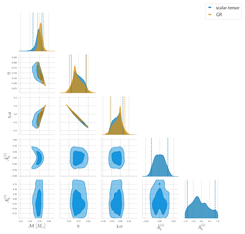
Figure 1: The posterior probability distributions of the phase parameters and the scalar radiation parameters, the chirp mass in the detector frame $\mathcal{M}$, the luminosity distance $d_{L}$, the inclination angle $\iota$, and the additional parameters due to scalar radiation $\tilde{A}^{(1)}_{b}$ and $A_{b}^{(1)}$, are shown in blue for GW200115 with 50% and 90% credible intervals in the 2-dimensional plots and 90% credible interval in the 1-dimensional plots. For comparison, the results under GR by LVK collaboration [5] are also shown in orange. The estimated mean values is $\tilde{A}^{(1)}_{b}=-0.001^{+0.029}_{-0.029}$ with 90% credible level.

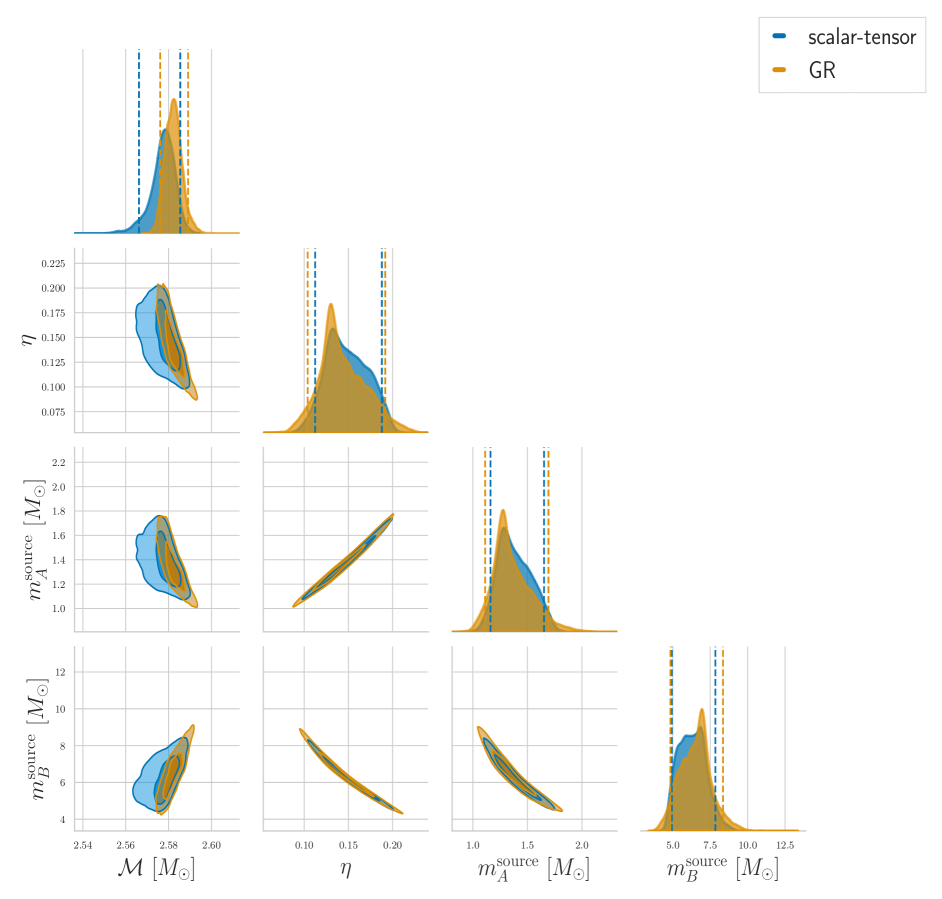
Figure 2: The posterior probability distributions of the mass parameters, the chirp mass in the detector frame $\mathcal{M}$, the symmetric mass ratio $\eta$, and the component masses in the source frame $m_{A}^{\rm source}$ and $m_{B}^{\rm source}$, are shown in blue for GW200115 with 50% and 90% credible intervals in the 2-dimensional plots and 90% credible interval in the 1-dimensional plots. For comparison, the results under GR by LVK collaboration [5] are also shown in orange.

Fig. 3 shows the posterior probability distribution of the amplitude parameters such as chirp mass in the detector frame $\mathcal{M}$, luminosity distance $d_{L}$, inclination angle $\iota$, and the additional scalar parameters $A^{(1)}_{b}$ and $\tilde{A}^{(1)}_{b}$ in blue. In corner plots, we draw 50% and 90% credible intervals in the 2-dimensional plots and 90% credible intervals in the 1-dimensional plots again. For comparison, we also show the posterior distribution estimated from the GR analysis by LVK collaboration [5] in orange. We do not find correlations between the phase parameter $\tilde{A}^{(1)}_{b}$, and the luminosity distance $d_{L}$ or the inclination angle $\iota$. However, there is little correlation of the scalar amplitude $A^{(1)}_{b}$ with the other amplitude parameters. Note that the inclusion of the scalar polarization seems to improve the inclination determination. We will discuss this point in detail at the end of this section by comparing the results based on different analytical settings. With the current detector sensitivity, it was found that some scalar amplitude samples hit the edge of the prior. However, since the 90% CL is inside the prior, we found the first constraint on the additional parameter purely characterizing scalar polarization amplitude

$$A^{(1)}_{b}=-0.16^{+0.83}_{-0.86}\,,$$ (94)

with 90% credible interval.

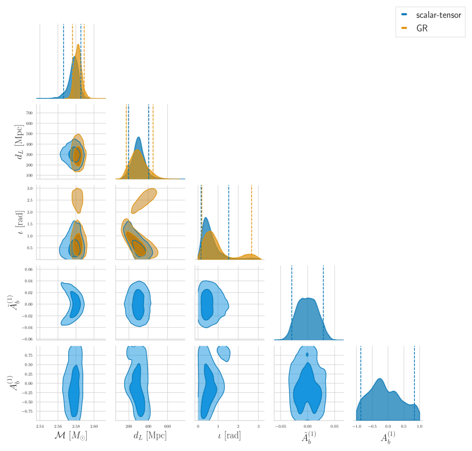
Figure 3: The posterior probability distributions of the amplitude parameters and the scalar polarization parameters: the chirp mass in the detector frame $\mathcal{M}$, the luminosity distance $d_{L}$, the inclination angle $\iota$, and the additional parameters due to scalar radiation $\tilde{A}_{b}^{(1)}$ and $A_{b}^{(1)}$, for GW200115 with 50% and 90% credible intervals in the 2D plots and 90% credible interval in the 1D plots. For comparison, the results under GR by LVK collaboration [5] are also shown in orange. We found little correlations with the amplitude parameters, the luminosity distance $d_{L}$ and the inclination angle $\iota$, and the scalar amplitude parameter $\tilde{A}_{b}^{(1)}$. The estimated mean value is $A_{b}^{(1)}=-0.16^{+0.83}_{-0.86}$ with 90% credible level. The constraint on the scalar amplitude $A^{(1)}_{b}$ can be converted into the constraint on the scalar-to-amplitude ratio defined by Eq. (107): $R^{(1)}_{ST}\leq 0.71$.

On using the correspondence (85) with the constraint on $\tilde{A}^{(1)}_{b}$ Eq. (92), the amplitude of $\hat{\alpha}_{A}$ is constrained to be

$$|\hat{\alpha}_{A}|\lesssim 0.04\,,$$ (95)

at 90% credible level. This gives the upper limit on the amount of the NS scalar charge in the mass range Eq. (93). The vanishing scalar charge ($\hat{\alpha}_{A}=0$) is consistent with the GW200115 data. On the other hand, on using the correspondence (84) on ${A}^{(1)}_{b}$ Eq. (94), the product $\xi_{0}\hat{\alpha}_{A}$ is constrained to be

$$-2.04<\xi_{0}\hat{\alpha}_{A}<1.34\,.$$ (96)

Compared to $\hat{\alpha}_{A}$, we only have a weak bound on the other parameter $\xi_{0}$. This is associated to the fact that the amplitude of the breathing polarization is poorly constrained with the GW200115 data. Fig. 4 shows the posterior distributions on two theoretical model parameters, the scalar charge $\hat{\alpha}_{A}$ and the nonminimal coupling strength converted from the samples of $\tilde{A}_{b}^{(1)}$ and $A_{b}^{(1)}$ through the relations (84). We put constraints on these scalar radiation parameters simultaneously only from the observation of the single compact binary coalsecence event. The estimated values are

$$\hat{\alpha}_{A} = -0.001^{+0.042}_{-0.042}\,,$$ (97)

$$\xi_{0} = -0.98^{+198}_{-197}\,,$$ (98)

with 90% credible intervals.

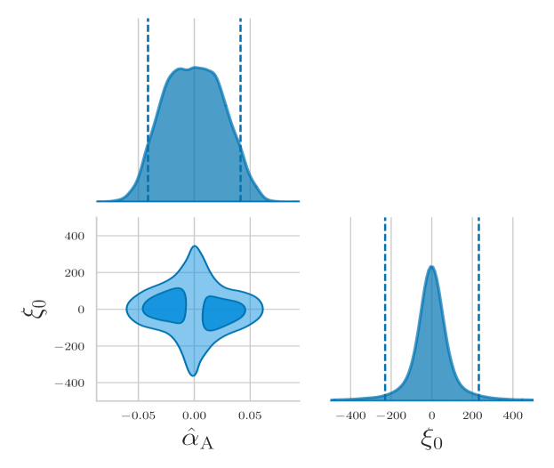
Figure 4: The posterior probability distributions of the additional phase correction $\tilde{A}_{b}^{(}1)$ and the scalar amplitudes $A_{b}^{(1)}$ for GW200115 with 50% and 90% credible intervals in the 2-dimensional plots and 90% credible interval in the 1-dimensional plots. The constraints on $\tilde{A}^{(1)}_{b}=-0.001^{+0.029}_{-0.029}$ and $A_{b}^{(1)}=-0.16^{+0.83}_{-0.86}$ when considering quadrupole scalar radiation can be converted into the bounds on the Horndeski parameters: $\hat{\alpha}_{A}=-0.001^{+0.042}_{-0.042}$ and $\xi_{0}=-0.98^{+198}_{-197}$ with 90% credible intervals. The sparse samples of $\hat{\alpha}_{A}\sim 0$ in the 2D plot is due to the fact that $\xi_{0}$ is so large for the samples around $\tilde{A}^{(1)}_{b}\sim 0$, where some samples are sparsely distributed outside the depicted region of the figure.

IV.2.2 Comparison with different waveform components

In order to assess the contribution of the amplitude and phase parts of each polarization mode to the posterior samples, we analyze GW200115 with two different settings of the waveform model: (i) tensor modes with scalar corrections and (ii) tensor modes plus scalar dipole mode.

Tensor modes with scalar phase corrections

First, we perform the Bayesian analysis based on the waveform model including only the tensor modes $\tilde{h}_{+,\times}$ with the amplitude and phase corrections due to scalar radiation. In this model, we do not consider the appearance of scalar polarization modes, Eqs. (78) and (79). Hence, the waveform model is given by

$$\tilde{h}_{I}(f)=\tilde{h}_{T}(f)\,,$$ (99)

where the GW polarizations are

$$\tilde{h}_{T}(f) = -\left[F_{I}^{+}(1+\cos^{2}{\iota})-2iF_{I}^{\times}\cos{\iota}\right]\sqrt{\frac{5\pi}{96}}\frac{(G_{*}{{\cal M}})^{2}}{d_{L}}\left(u_{*}^{(2)}\right)^{-7/2}e^{-i\Psi_{\text{GR}}^{(2)}}e^{-i\delta\Psi^{(2)}}\,,$$ (100)

with the phase corrections

$$\delta\Psi^{(\ell)} =-\frac{5\ell}{3584}\left(\tilde{A}_{b}^{(1)}\right)^{2}\eta^{2/5}\left(u_{*}^{(\ell)}\right)^{-7}-\frac{\ell}{128}\left(\tilde{A}_{b}^{(2)}\right)^{2}\left(u_{*}^{(\ell)}\right)^{-5}\;.$$ (101)

This reduced waveform model imitates the parameterized tests for the inspiral GWs performed by LVK collaboration [9]. The difference between this reduced analysis and the parameterized tests by the LVK collaboration is essentially the prior setting for the phase deviation parameter. In our model, we adopt a uniform prior for $\tilde{A}^{(1)}_{b}$, but they use a uniform prior on $\varphi_{-2}$, which is corresponding to $\sim(\tilde{A}^{(1)}_{b})^{2}$. Hence, we can evaluate the contribution of the existence of scalar polarization itself to the parameter estimation by comparing this analysis with the results of the scalar-tensor model. Fig. 5 shows the comparison of the posterior samples for the phase parameters between the scalar-tensor model (blue) and the model of tensor modes with scalar corrections (orange).

By considering scalar modes, the phase parameters appear to be better estimated. The estimated mean value is $|\tilde{A}^{(1)}_{b}|\leq 0.034$ with 90% credible level, which can be converted into $|\hat{\alpha}_{A}|\leq 0.049$ through Eq. (85). Thus, we expect that the inclusion of the scalar polarization modes would break the parameter degeneracy. Figure 6 shows the comparison of the posterior samples for the amplitude parameters between the scalar-tensor model (blue) and the model of tensor modes with scalar corrections (orange). We note that the posterior distribution for the inclination angle $\iota$ changes by including the scalar modes and the gradual peak around $\iota\sim 2.5\ {\rm rad}$ has disappeared. We can also find the similar two peaks in the GR analysis as shown in orange in Fig. 3. The inclination-angle dependence of the GW radiation differ among the polarization modes [106]. The overall inclination-angle dependence of the tensor modes is given by $\sqrt{(1+\cos^{2}{\iota})^{2}+4\cos^{2}{\iota}}$, which has similar values at the positions of the two peaks $\iota\sim 0.5\ {\rm rad}$ and $\iota\sim 2.5\ {\rm rad}$. However, since the dipole scalar mode is proportional to $\sin{\iota}$, the sign of the amplitude flips between the two peaks. Thus, the inclination dependence of the dipole scalar mode in the waveform model would be helpful to break the partial degeneracy in the inclination angle. It would result in the better constraints on the other parameters.

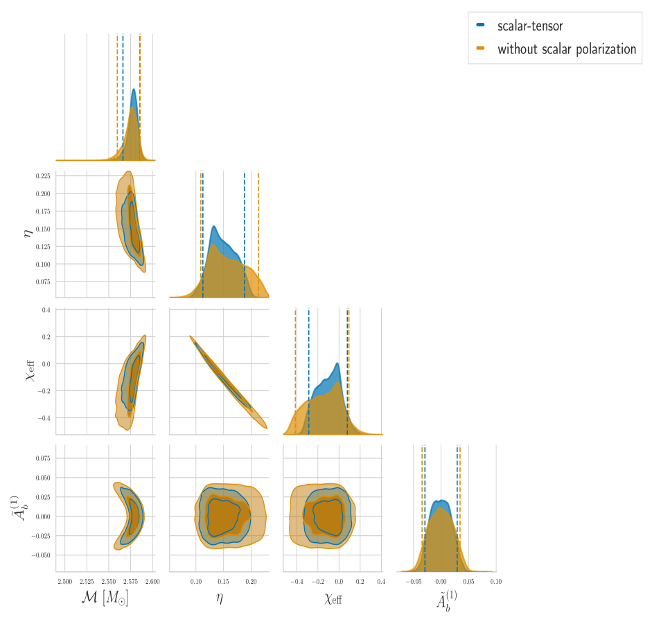
Figure 5: This is a similar figure to Fig. 1 but compared to the analysis using the model of tensor modes with scalar phase corrections. The estimated mean values is $|\tilde{A}^{(1)}_{b}|\leq 0.034$ with 90% credible level in comparison with $|\tilde{A}^{(1)}_{b}|\leq 0.029$ for the scalar-tensor model.

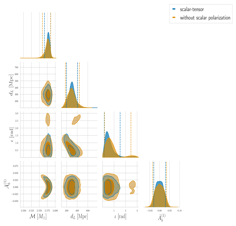
Figure 6: This is a similar figure to Fig. 3 but compared to the analysis using the model of tensor modes with scalar phase corrections.

Tensor modes plus scalar dipole mode

Second, we perform the Bayesian analysis based on the waveform model including the tensor modes $\tilde{h}_{+,\times}$, dipole scalar mode $\tilde{h}_{b1}$, and the amplitude and phase corrections due to the dipole scalar radiation. Hence, the waveform model is given by

$$\tilde{h}_{I}(f)=\tilde{h}_{T}(f)+\tilde{h}^{(1)}_{b}(f)\,,$$ (102)

where the GW polarizations are

$$\tilde{h}_{T}(f) = -\left[F_{I}^{+}(1+\cos^{2}{\iota})-2iF_{I}^{\times}\cos{\iota}\right]\left[1+\delta A^{(2)}\right]\sqrt{\frac{5\pi}{96}}\frac{(G_{*}{{\cal M}})^{2}}{d_{L}}\left(u_{*}^{(2)}\right)^{-7/2}e^{-i\Psi_{\text{GR}}^{(2)}}e^{-i\delta\Psi^{(2)}}\,,$$ (103)

$$\tilde{h}^{(1)}_{b}(f) = \sqrt{\frac{5\pi}{48}}A^{(1)}_{b}F_{I}^{b}(2\sin{\iota})\eta^{1/5}\frac{(G_{*}{\cal M})^{2}}{d_{L}}\left(u_{*}^{(1)}\right)^{-9/2}e^{-i\Psi_{\text{GR}}^{(1)}}e^{-i\delta\Psi^{(1)}}\,,$$ (104)

with the phase corrections

$$\delta A^{(\ell)}=-\frac{5}{48}\left(\tilde{A}_{b}^{(1)}\right)^{2}\eta^{2/5}\left(u_{*}^{(\ell)}\right)^{-2}\,,$$ (105)

$$\delta\Psi^{(\ell)}=-\frac{5\ell}{3584}\left(\tilde{A}_{b}^{(1)}\right)^{2}\eta^{2/5}\left(u_{*}^{(\ell)}\right)^{-7}\;.$$ (106)

In this model, we omit the quadrupole scalar radiation because we expect that the dipole radiation becomes dominant at the early inspiral stage. Hence, we can evaluate the contribution of the scalar quadrupole mode to the parameter estimation by comparing the result of this analysis with that using the scalar-tensor model. Fig. 7 shows the comparison of the posterior samples for the phase parameters and Fig. 8 shows the comparison of the posterior samples for the amplitude parameters between the scalar-tensor model (blue) and the model of tensor modes plus scalar dipole mode (orange). The posterior distributions for both are almost identical. This indicates that the results of the current analysis in scalar-tensor are mostly determined by the corrections due to scalar dipole radiation.

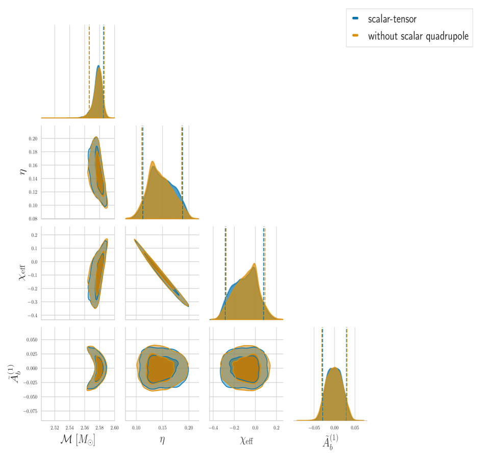
Figure 7: This is a similar figure to Fig. 1 but compared to the analysis using the model of tensor modes plus scalar dipole mode.

Figure 8: This is a similar figure to Fig. 3 but compared to the analysis using the model of tensor modes plus scalar dipole mode.

IV.2.3 Scalar-to-tensor amplitude ratio

We define scalar-to-tensor amplitude ratios as the ratios of scalar-mode amplitude to tensor-mode amplitude, that is, from Eqs. (77) – (79),

$$R^{(1)}_{ST}\equiv\left|\frac{A^{(1)}_{b}\eta^{1/5}\sin\iota}{\sqrt{(1+\cos^{2}\iota)^{2}+4\cos^{2}\iota}}(G_{*}\mathcal{M}\pi f)^{-1/3}\right|\,,$$ (107)

for the scalar dipole mode and

$$R^{(2)}_{ST}\equiv\left|\frac{A^{(2)}_{b}2\sin^{2}\iota}{\sqrt{(1+\cos^{2}\iota)^{2}+4\cos^{2}\iota}}\right|\,,$$ (108)

for the scalar quadrupole mode. This ratio is an observational indicator to represent how deep the scalar mode is explored by the GW observation compared to the tensor modes. As shown in Section IV.2, since the contribution of the dipole scalar mode is dominant and the dipole mode amplitude and the quadrupole mode are characterized by the same parameter $A^{(1)}_{b}$, we evaluate the dipole scalar-to tensor amplitude ratio here. On substituting the estimated mean values and the 90% credible intervals for the parameters $\mathcal{M}$, $\iota$, $A^{(1)}_{b}$ and the typical GW frequency $f\sim 100\ {\rm Hz}$, we find the constraints on the ratio as

$$R^{(1)}_{\rm ST}\lesssim 0.71\,,$$ (109)

for GW200115. This scalar-to-tensor amplitude ratio is relatively large compared to the ratios for GW170814 and GW170817 reported in [101]. As the values of $|\sin\iota|$ and $|\cos\iota|$ are similar to those of the previous events, the reason is because the authors assumed that the coupling $\gamma$ in Eq. (73) is unity, and then the scalar-mode amplitude is determined by the phase evolution of the tensor modes. On the other hand, the constraint (109) is purely determined by the ability of the GW detector network to probe into the scalar mode. Therefore, this constraint on the scalar-to-tensor amplitude ratio means that the current GW detector network is able to probe into the scalar mode at a level that is at most slightly better than the amplitude of the tensor modes.

V Theoretical interpretation of GW200115 constraints

Let us interpret the observational bounds (97) and (98) as the constraints on model parameters of theories encompassed by the action (1). We will consider two theories: (A) BD theories with the functions (2), and (B) theories of spontaneous scalarization of NSs with the functions (4).

For this purpose, we first revisit how $\hat{\alpha}_{A}$ is approximately related to the nonminimal coupling and the NS EOS. On a static and spherically symmetric background, the large-distance solution far outside the NS is given by Eq. (19), where $q_{s}$ is related to $\hat{\alpha}_{A}$ according to Eq. (20). In the Jordan frame, the radial distance $r$ and the NS ADM mass $m_{A}$ can be expressed as $r=\hat{r}/\sqrt{F(\phi)}$ and $m_{A}=\hat{m}_{A}\sqrt{F(\phi)}$, respectively, where $F(\phi)$ is the nonminimal coupling. Then, the scalar-field solution at large distances is given by

$$\phi(r)=\phi_{0}-\frac{m_{A}\hat{\alpha}_{A}}{4\pi M_{\rm Pl}F(\phi_{0})}\frac{1}{r}\,.$$ (110)

The scalar-field solution expanded around $r=0$ up to the order of $r^{2}$ is [66]

$$\phi(r)=\phi_{c}-\frac{\xi_{c}\rho_{c}}{12F(\phi_{c})M_{\rm Pl}}(1-3w_{c})r^{2}\,,$$ (111)

where $\phi_{c}$ and $\rho_{c}$ are the field value and the matter density at $r=0$, respectively, and $w_{c}=P_{c}/\rho_{c}$ is the EOS parameter at $r=0$ with the central pressure $P_{c}$, and

$$\xi_{c}\equiv\frac{M_{\rm Pl}F_{,\phi}}{F}\biggl{|}_{\phi=\phi_{c}}\,.$$ (112)

The solution (111) loses its validity around the NS surface ($r=r_{s}$), but we may extrapolate this solution up to $r=r_{s}$. Extrapolating also the large-distance solution (110) down to $r=r_{s}$ and matching its radial derivative with that of Eq. (111), we obtain the relation

$$\hat{\alpha}_{A}\simeq-\frac{\xi_{c}}{2}(1-3w_{c})\,,$$ (113)

where we used the approximations $F(\phi_{c})\simeq F(\phi_{0})$ and $m_{I}\simeq 4\pi\rho_{c}r_{s}^{3}/3$. The formula (113) is a crude estimation, but it is useful to understand what determines the scalar charge. Not only the nonminimal coupling strength $\xi_{c}$ but also the NS EOS $w_{c}$ affects the amplitude of $\hat{\alpha}_{I}$. As we approach $r=r_{s}$ from $r=0$, the matter EOS parameter $w=P/\rho$ (with pressure $P$ and density $\rho$) decreases toward 0. This means that, for $w_{c}<1/3$, the formula (113) can underestimate the amplitude of $\hat{\alpha}_{I}$. Moreover, the $\mu(\phi)X^{2}$ term in $G_{2}$ does not affect the expansion (111) up to the order of $r^{2}$ by reflecting the fact that the leading-order field derivative around $r=0$ is the term linear in $X$ (i.e., $\phi^{\prime}(r)\propto r$). However, as $r$ approaches $r_{s}$, we cannot neglect the higher-order term $\mu(\phi)X^{2}$ relative to $X$. This effect modifies the solution to the scalar field especially around $r=r_{s}$. When $\mu(\phi)$ is negative, there is a kinetic screening of $\phi^{\prime}(r)$, which leads to the suppression of $|\hat{\alpha}_{A}|$ [66].

V.1 BD theories

In BD theories, the nonminimal coupling is given by $F(\phi)=e^{-2Q\phi/M_{\rm Pl}}$. In this case, the quantities $\xi_{0}$ and $\xi_{c}$ reduce to

$$\xi_{0}=\xi_{c}=-2Q\,,$$ (114)

which do not depend on $\phi$. The bound (98) translates to

$$|Q|\leq 99\,,$$ (115)

which is weak due to the poorly constrained value of the nonminimal coupling strength $\xi_{0}$.

On using the approximate relation (113), we have

$$\hat{\alpha}_{A}\simeq Q(1-3w_{c})\,.$$ (116)

Applying the bound (97) to this approximate relation, the coupling constant $Q$ is constrained to be

$$|Q|\lesssim\frac{0.04}{1-3w_{c}}\,.$$ (117)

If we take the EOS parameter $w_{c}=0.2$ as a typical value, the bound (117) crudely translates to $|Q|\lesssim 0.1$.

Since we do not know the precise NS EOS of the GW200115 event, there is an uncertainty of the upper limit on $|Q|$. By specifying a particular EOS, $\hat{\alpha}_{A}$ can be numerically computed without resorting to the approximate formula (116). We use an analytic representation of the SLy EOS given in Ref. [118]. We numerically calculate $\hat{\alpha}_{A}$ by changing the values of $Q$ and the central matter density $\rho_{c}$. In Fig. 9, we plot $\hat{\alpha}_{A}$ versus the NS mass $m_{A}$ (normalized by $M_{\odot}$) for four positive values of $Q$. Since $m_{A}$ tends to increase for larger $w_{c}$ in the range $w_{c}<1/3$, the approximate relation (116) implies that $\hat{\alpha}_{A}$ should decrease as a function of $m_{A}$. Indeed, this behavior of $\hat{\alpha}_{A}$ versus $m_{A}$ can be confirmed in Fig. 9. We note that, for $w_{c}$ exceeding $1/3$, the approximate formula (116) loses its validity. Even in such cases, the numerical values of $\hat{\alpha}_{A}$ are typically positive for $Q>0$.

In Fig. 9, we show the GW200115 bound $\hat{\alpha}_{A}\leq 0.041$ besides the region of $m_{A}$ constrained from the data, i.e., $1.16M_{\odot}\leq m_{A}\leq 1.65M_{\odot}$. Requiring that the theoretical curves are within the region constrained from the GW 200115 data, we obtain the bound

$$|Q|\leq 0.055\,,\qquad{\rm or}\qquad\omega_{\rm BD}\geq 81\,\qquad{\rm for~{}~{}SLy~{}EOS}\,,$$ (118)

This is tighter than the crude estimation $|Q|\lesssim 0.1$ explained above. In the analysis of tensor modes alone without the breathing scalar mode, which is similar to the analysis performed in Refs. [9, 88], we find that the constraint on the scalar charge becomes looser, i.e., $|\hat{\alpha}_{A}|\leq 0.049$. In this case, the bound on the BD parameter is consistent with the limit $\omega_{\rm BD}\gtrsim 40$ derived in Ref. [88]. The breaking of the partial parameter degeneracy by adding the scalar mode would contribute to the tighter bound. We recall that, even for $\hat{\alpha}_{A}<0$, the observational upper limit of $|\hat{\alpha}_{A}|$ in Eq. (97) is similar to that for $\hat{\alpha}_{A}>0$. Hence, for $Q<0$, we also obtain the bound on $|Q|$ similar to (118). Although they are weaker than the limit $|Q|\leq 2.5\times 10^{-3}$ [25, 26, 12] constrained from the solar-system tests by one order of magnitude, it is expected that future high-precision GW observations can put tighter bounds on $|Q|$.

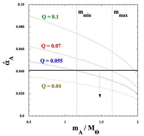
Figure 9: The scalar charge $\hat{\alpha}_{A}$ versus the NS mass $m_{A}$ (normalized by the solar mass $M_{\odot}$) for the SLy EOS in BD theories with four different couplings $Q$. We also show the upper limit $\hat{\alpha}_{A}=0.041$ constrained from the GW200115 data as a bold black line. The two dashed lines correspond to the minimum and maximum NS masses ($m_{\rm min}=1.16M_{\odot}$ and $m_{\rm max}=1.65M_{\odot}$) constrained from the data. Since the theoretical curves need to be in the ranges $\hat{\alpha}_{A}\leq 0.041$ and $m_{\rm min}\leq m_{A}\leq m_{\rm max}$, the coupling $Q$ is bounded as $Q\leq 0.055$.

V.2 Theories of spontaneous scalarization of NSs

In theories of NS spontaneous scalarization with the nonminimal coupling $F(\phi)=e^{-\beta\phi^{2}/(2M_{\rm Pl}^{2})}$, the nonminimal coupling strength far outside the NS is given by

$$\xi_{0}=-\frac{\beta\phi_{0}}{M_{\rm Pl}}\,.$$ (119)

Then, the bound (98) translates to

$$|\beta\phi_{0}|\leq 198M_{\rm Pl}\,.$$ (120)

In current theories, the parameterized post-Newtonian (PPN) parameter $\gamma_{\rm PPN}$ is given by $\gamma_{\rm PPN}-1=-2\xi_{0}^{2}/(2+\xi_{0}^{2})$ [90, 47]. Then, the solar-system constraint $\gamma_{\rm PPN}-1=(2.1\pm 2.3)\times 10^{-5}$ [6] translates to $|\beta\phi_{0}|\leq 1.4\times 10^{-3}M_{\rm Pl}$. The current limit (120) arising from the amplitude of scalar GWs is much weaker than the solar-system bound.

V.2.1 DEF model

Let us first consider the original DEF model with $\mu(\phi)=0$ in the coupling functions (4). In this case, we can crudely estimate the scalar charge by using Eq. (113) as

$$\hat{\alpha}_{A}\simeq\frac{\beta\phi_{c}}{2M_{\rm Pl}}(1-3w_{c})\,,$$ (121)

which depends on the field value $\phi_{c}$ and the NS EOS $w_{c}$ around $r=0$. Spontaneous scalarization of NSs occurs for $\beta\leq-4.35$ due to the tachyonic instability of the GR branch ($\phi=0$). This critical value of $\beta$ is insensitive to the choices of NS EOSs [48, 49, 50, 51]. When spontaneous scalarization occurs, the field value $\phi_{c}$ can be as large as ${\cal O}(0.1M_{\rm Pl})$. Then, the estimation (121) shows that $|\hat{\alpha}_{A}|$ should reach the order $0.1$. Since the amplitude of $\hat{\alpha}_{A}$ depends on the coupling constant $\beta$, it is possible to put constraints on $\beta$ by using the observational bound (97). The scalar charge $\hat{\alpha}_{A}$ also carries the information of NS EOSs, but, for given $\beta$, the maximum values of $|\hat{\alpha}_{A}|$ weakly depend on the choices of NS EOSs [48, 49, 50, 51, 88].

For the SLy EOS, we numerically compute $\hat{\alpha}_{A}$ by choosing several different values of $\beta$. For given $\beta$ and $\rho_{c}$, we will iteratively find a boundary value of $\phi_{c}$ leading to a scalarized solution with the asymptotic field value $\phi_{0}$ close to 0 (to be consistent with the solar-system bound mentioned above). Different choices of $\rho_{c}$ lead to different NS masses and scalar charges. Spontaneous scalarization of NSs occurs for intermediate central densities $\rho_{c}$, in which regime $\hat{\alpha}_{A}$ is nonvanishing.

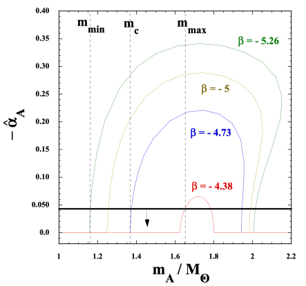
Figure 10: We plot $-\hat{\alpha}_{A}$ versus the NS mass $m_{A}$ (normalized by the solar mass $M_{\odot}$) for the SLy EOS in original DEF theories of spontaneous scalarization. We choose four different coupling constants: $\beta=-5.26,-5,-4.73,-4.38$. The upper limit $-\hat{\alpha}_{A}=0.043$ constrained from the GW200115 data is plotted as a bold black line. We also show the minimum, maximum, and central NS masses as three dashed lines, which are $m_{\rm min}=1.162M_{\odot}$, $m_{\rm max}=1.652M_{\odot}$, and $m_{c}=1.368M_{\odot}$, respectively. The observationally allowed region corresponds to a rectangle characterized by $0\leq-\hat{\alpha}_{A}\leq 0.043$ and $m_{\rm min}\leq m_{A}\leq m_{\rm max}$.

In Fig. 10, we show $-\hat{\alpha}_{A}$ versus $m_{A}/M_{\odot}$ for four different values of $\beta$ with the choice of the SLy EOS. Since $\beta<0$ for the occurence of scalarization, $\hat{\alpha}_{A}$ is negative if $\phi_{c}>0$. For $\beta=-5.26$, spontaneous scalarization occurs for the mass range $1.16M_{\odot}\leq m_{A}\leq 2.01M_{\odot}$. In the rest of the mass region, the scalar charge is vanishing ($\hat{\alpha}_{A}=0$). For $\beta<-5.26$, the theoretical curve is outside the observationally allowed region ($0\leq-\hat{\alpha}_{A}\leq 0.043$) for any NS mass constrained from the GW200115 event ($1.162M_{\odot}\leq m_{A}\leq 1.652M_{\odot}$). Then, we obtain the bound

$$\beta\geq-5.26\,,$$ (122)

for the SLy EOS. As $\beta$ increases, the mass region in which scalarization takes places gets narrower, with smaller maximum values of $|\hat{\alpha}_{A}|$. For $-5.26\leq\beta\leq-4.38$, there are the mass ranges excluded by the observational limit $|\hat{\alpha}_{A}|\leq 0.043$, together with the existence of allowed mass parameters within the mass range of the GW200115 event. As $\beta$ increases toward $-4.38$, the observationally excluded mass region tends to be narrower. In particular, the model with $\beta\geq-4.38$ is consistent with the bound on $\hat{\alpha}_{A}$ for all the constrained mass ranges. This is much stronger than the constraint (122), but we have to caution that there are still allowed mass regions even for $-5.26\leq\beta\leq-4.38$. In this sense, we will take the conservative limit (122) as the bound on $\beta$ constrained from the GW200115 data.

Clearly, the observational uncertainty of the NS mass gives the limitation for putting tight bounds on $\beta$. Let us take the central value of $m_{A}$ constrained from the data, i.e., $m_{c}=1.368M_{\odot}$. If we demand the condition $|\hat{\alpha}_{A}|\leq 0.043$ in this case, the coupling needs to be in the range

$$\beta\geq-4.73\,,\qquad{\rm for}\quad m_{A}=1.368M_{\odot}\,.$$ (123)

This shows that, if the NS mass is constrained to be in a narrower range, it is possible to place tighter bounds on $\beta$ than (122). Since this can happen in future observations, the accumulation of many NS-BH merger events will clarify whether the original spontaneous scalarization scenario is excluded or not. Combined with the condition for the occurenece of spontaneous scalarization, the coupling $\beta$ is now constrained to be $-5.26\leq\beta\leq-4.35$. Hence the allowed range of $\beta$ is already narrow even with a single GW event. We note that, in the analysis of Ref. [75], the authors extended the range of $\beta$ to $\beta>-4.35$ in which spontaneous scalarization does not occur. In this regime, the solution stays in the GR branch $\phi(r)=0$ and hence $\hat{\alpha}_{A}=0$. In this sense, the constraint on $\beta$ in the scalarization scenario is meaningful only for $\beta\leq-4.35$.

V.2.2 DEF model with kinetic screening

Let us next proceed to the case in which there is a term $\mu_{2}X^{2}$ in the function $G_{2}$ of Eq. (4), i.e., $\mu(\phi)=\mu_{2}={\rm constant}$. For $\mu_{2}<0$, it was shown in Ref. [66] that the higher-order derivative term can lead to a kinetic screening of the scalar field inside the NS. As we see in Fig. 11, the scalar charge $|\hat{\alpha}_{A}|$ tends to be smaller for decreasing values of $\mu_{2}$. The NS mass range in which spontaneous scalarization occurs is insensitive to the coupling constant $\mu_{2}$. In other words, the maximum values of $|\hat{\alpha}_{A}|$ get smaller for decreasing $\mu_{2}$, but the mass range with $|\hat{\alpha}_{A}|>0.01$ is hardly modified. This properly is different from the spontaneous scalarization scenario with $\mu_{2}=0$, in which case the mass region with $|\hat{\alpha}_{A}|>0.01$ shrinks for increasing $\beta$ (see Fig. 10).

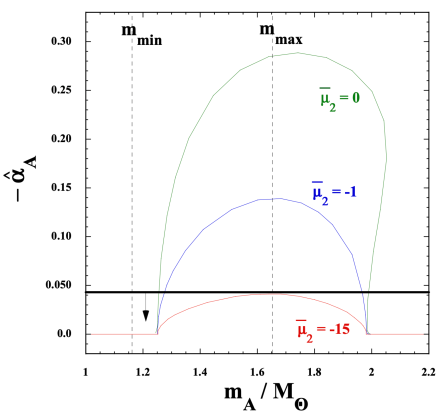
Figure 11: $-\hat{\alpha}_{A}$ versus $m_{A}/M_{\odot}$ for the SLy EOS in theories of spontaneous scalarization with $\beta=-5$ in the presence of the higher-order derivative term $\mu_{2}X^{2}$. Each line corresponds to $\bar{\mu}_{2}=0,-1,-15$ from top to bottom, where $\bar{\mu}_{2}=\mu_{2}M_{\rm Pl}^{2}/r_{0}^{2}$ with $r_{0}=89.664$ km. We also show the observational limits of $-\hat{\alpha}_{A}$ and $m_{A}$. For $\bar{\mu}_{2}\leq-15$, the theoretical lines are within the region constrained from the data.

As an example, let us consider the case where $\beta=-5$. Then, the condition (122) is satisfied in the original scalarization scenario, but there are the NS mass ranges in which the inequality $|\hat{\alpha}_{A}|\leq 0.043$ is violated. Indeed, for the medium mass $m_{A}=1.368M_{\odot}$, this bound on $\hat{\alpha}_{A}$ is not satisfied, see Eq. (123). In Fig. 11, we plot $-\hat{\alpha}_{A}$ versus $m_{A}$ for $\bar{\mu}_{2}=0,-1,-15$ by fixing $\beta=-5$, where $\bar{\mu}_{2}\equiv\mu_{2}M_{\rm Pl}^{2}/r_{0}^{2}$ and $r_{0}=89.664$ km. The theoretical curves are within the observationally constrained region of $\hat{\alpha}_{A}$ and $m_{A}$ if

$$\bar{\mu}_{2}\leq-15\,,\qquad{\rm for}\quad\beta=-5\,.$$ (124)

Thus, even for $\beta=-5$, the kinetic screening induced by the higher-order derivative term $\mu_{2}X^{2}$ leads to the compatibility with the GW200115 data for all the constrained mass ranges. Thus, for $\mu_{2}<0$, the allowed parameter region of $\beta$ is not restricted to be small unlike the DEF model with $\mu_{2}=0$.

VI Conclusions

From the NS-BH merger event GW200115, we have placed observational constraints on the NS scalar charge and the nonminimal coupling strength. For this purpose, we chose a subclass of Horndeski theories given by the action (1), in which case the speed of gravity is luminal. In such theories the BHs are not endowed with scalar hairs, but it is possible for the NSs to have hairy solutions through a scalar-matter interaction induced by the nonminimal coupling $G_{4}(\phi)R$. The representative examples are BD theories and theories of spontaneous scalarization given by the Horndeski functions (2) and (4), respectively.

In theories given by the action (1), the inspiral gravitational waveforms emitted from compact binaries were computed in Ref. [66]. In Sec. II, we reviewed the derivation of time-domain GW solutions by assuming that the scalar field is massless. In this case, there are two tensor polarizations $h_{+}$ and $h_{\times}$ besides a breathing mode $h_{b}$ arising from the scalar-field perturbation. Focusing on a NS-BH binary system in which the BH has a vanishing scalar charge, we derived the waveforms of frequency-domain GWs propagating on the cosmological background. They are given by Eqs. (64)-(66) with the amplitudes (67)-(69) and phases (70)-(71). In particular, the breathing mode in the frequency domain is newly obtained in this paper.

In Sec. III, we provided a parameterized scalar-tensor waveform model starting with a modified energy flux. Our parameterized waveforms include not only the corrections for the tensor modes stemming from scalar radiation but also the scalar polarization modes itself. Originally, the model includes four additional parameters. The two parameters $A_{b}^{(1)}$ and $A_{b}^{(2)}$ represent the amplitudes of dipole and quadrupole scalar polarizations, and the two parameters $\tilde{A}_{b}^{(1)}$ and $\tilde{A}_{b}^{(2)}$ characterize the waveform corrections due to the dipole and quadrupole scalar radiation. Since the parameterized waveform model encompasses the theoretical waveforms derived in the underlying scalar-tensor theory, we also provided the correspondence between the parametrized waveforms and the theoretical waveforms. According to the correspondence, the two parameters $A_{b}^{(1)}$ and $\tilde{A}_{b}^{(1)}$ can be expressed in terms of the NS scalar charge $\hat{\alpha}_{A}$ and the nonminimal coupling strength $\xi_{0}$, as $A_{b}^{(1)}=\xi_{0}\hat{\alpha}_{A}/2$ and $\tilde{A}_{b}^{(1)}=\hat{\alpha}_{A}/\sqrt{2}$. The remaining two parameters $A_{b}^{(2)}$ and $\tilde{A}_{b}^{(2)}$ are given by multiplying $A_{b}^{(1)}$ and $\tilde{A}_{b}^{(1)}$ by a factor depending on the mass ratio. Thus, we have two additional free parameters $A_{b}^{(1)}$ and $\tilde{A}_{b}^{(1)}$, which can be constrained from the GW observations, in the subclass of Horndeski theories.

In Sec. IV, we placed observational bounds on the two model parameters $\hat{\alpha}_{A}$ and $\xi_{0}$ through the constraints on $A_{b}^{(1)}$ and $\tilde{A}_{b}^{(1)}$ achieved by the analysis of the GW200115 signal. The crucial difference from past works is that we have implemented the breathing scalar mode besides the two tensor polarizations. The inclination angle dependence of the scalar mode may break the partial degeneracy in the estimation of the inclination angle and improve the precision of the determination of the other parameters. The quantity $\hat{\alpha}_{A}$ appears in the phases of tensor waves at $-1$PN order. This property allows us to put the tight bound $\hat{\alpha}_{A}=-0.001^{+0.042}_{-0.042}$ from the GW200115 data, so that the amplitude of the scalar charge is bounded as $|\hat{\alpha}_{A}|\lesssim 0.04$. The amplitude of scalar GWs relative to tensor waves can put an upper limit on the product $\xi_{0}\hat{\alpha}_{A}$. Reflecting the weak observational sensitivity of scalar waves in current measurements, we obtained the loose bound $-2.04<\xi_{0}\hat{\alpha}_{A}<1.34$. Combining this with the limit on $\hat{\alpha}_{A}$, the nonminimal coupling strength is also weakly constrained to be $\xi_{0}=-0.98^{+198}_{-197}$. We note that the NS mass is constrained to be in the range $1.16M_{\odot}<m_{A}<1.65M_{\odot}$ from the GW200115 data.

In Sec. V, we translated the theoretical bounds on $\hat{\alpha}_{A}$ and $\xi_{0}$ into the constraints on model parameters in theories with the Horndeski functions (2) and (4). In BD theories, the parameter $\xi_{0}$ is simply equivalent to the coupling constant $-2Q$, so that the observational constraint on $\xi_{0}$ alone gives a weak limit $|Q|<99$. On the other hand, the other parameter $\hat{\alpha}_{A}$ depends on both $Q$ and the NS EOS. Extrapolating the solutions around $r=0$ and at large distances at the NS surface, we obtained the crude formula $\hat{\alpha}_{A}\simeq Q(1-3w_{c})$. On using the upper limit $|\hat{\alpha}_{A}|\lesssim 0.04$ and taking a typical value $w_{c}=0.2$, $|\hat{\alpha}_{A}|$ is smaller than the order 0.1. We numerically computed the values of $|\hat{\alpha}_{A}|$ for the SLy EOS without using the above approximation and derived the observational bound $|Q|\leq 0.055$, or equivalently, $\omega_{\rm BD}\geq 81$.

In the DEF model of spontaneous scalarization, $|\hat{\alpha}_{A}|$ can be as large as the order 0.1 depending on the coupling constant $\beta$. Provided that $\beta\geq-5.26$, there are the observationally constrained NS mass ranges in which the condition $|\hat{\alpha}_{A}|\leq 0.043$ is satisfied. Taking the central value of $m_{A}$ constrained from the data ($m_{A}=1.368M_{\odot}$), the bound on $\hat{\alpha}_{A}$ translates to $\beta\geq-4.73$. Due to the uncertainty of the NS mass, we take the most conservative bound $\beta\geq-5.26$ as a firm constraint extracted from the GW200115 data. Since the spontaneous scalarization occurs for $\beta\leq-4.35$, our newly derived bound already restricts the viable parameter space of $\beta$ to a narrow region. If we take into account the higher-order kinetic term $\mu_{2}X^{2}$ with $\mu_{2}<0$, the kinetic screening mechanism works to reduce $|\hat{\alpha}_{A}|$ without changing the scalarized NS mass region much. Taking the nonminimal coupling constant $\beta=-5$, the scalarization model with $\mu_{2}M_{\rm Pl}^{2}/r_{0}^{2}\leq-15$ is compatible with the GW200115 bound for all the constrained NS mass ranges.

We have thus shown that the NS-BH merger event GW200115 allows us to probe the property of hairy NS solutions. In particular, the observational constraint on the scalar charge $|\hat{\alpha}_{A}|\lesssim 0.04$ gives new bounds on the nonminimal coupling constants of BD theories and spontaneous scalarization scenarios with/without the kinetic screening. Furthermore, our analysis of the parameterized waveforms with scalar modes indicates that the presence of polarization modes beyond GR must be taken into account when attempting to interpret the results of parameterized tests with a specific theory of gravity. Otherwise, observational constraints on alternative theories of gravity may be biased. If the future GW observations were to reach the upper limit of $|\hat{\alpha}_{A}|$ below the order 0.01 with tighter constraints on $m_{A}$, it will be potentially possible to rule out the DEF model. Moreover, the increased sensitivity for measuring the amplitude of scalar GWs relative to tensor GWs will allow us to put tighter constraints on the nonminimal coupling strength $\xi_{0}$ [87].

References

- Abbott et al. [2016] B. P. Abbott et al. (LIGO Scientific, Virgo), Phys. Rev. Lett. 116, 061102 (2016), arXiv:1602.03837 [gr-qc] .
- Abbott et al. [2021a] R. Abbott et al. (LIGO Scientific, VIRGO, KAGRA), arXiv:2111.03606 [gr-qc] .
- Abbott et al. [2017] B. P. Abbott et al. (LIGO Scientific, Virgo, Fermi-GBM, INTEGRAL), Astrophys. J. Lett. 848, L13 (2017), arXiv:1710.05834 [astro-ph.HE] .
- Goldstein et al. [2017] A. Goldstein et al., Astrophys. J. Lett. 848, L14 (2017), arXiv:1710.05446 [astro-ph.HE] .
- Abbott et al. [2021b] R. Abbott et al. (LIGO Scientific, KAGRA, VIRGO), Astrophys. J. Lett. 915, L5 (2021b), arXiv:2106.15163 [astro-ph.HE] .
- Will [2014] C. M. Will, Living Rev. Rel. 17, 4 (2014), arXiv:1403.7377 [gr-qc] .
- Hoyle et al. [2001] C. D. Hoyle, U. Schmidt, B. R. Heckel, E. G. Adelberger, J. H. Gundlach, D. J. Kapner, and H. E. Swanson, Phys. Rev. Lett. 86, 1418 (2001), arXiv:hep-ph/0011014 .
- Adelberger et al. [2003] E. G. Adelberger, B. R. Heckel, and A. E. Nelson, Ann. Rev. Nucl. Part. Sci. 53, 77 (2003), arXiv:hep-ph/0307284 .
- Abbott et al. [2021c] R. Abbott et al. (LIGO Scientific, VIRGO, KAGRA), arXiv:2112.06861 [gr-qc] .
- Bertone et al. [2005] G. Bertone, D. Hooper, and J. Silk, Phys. Rept. 405, 279 (2005), arXiv:hep-ph/0404175 .
- Copeland et al. [2006] E. J. Copeland, M. Sami, and S. Tsujikawa, Int. J. Mod. Phys. D 15, 1753 (2006), arXiv:hep-th/0603057 .
- De Felice and Tsujikawa [2010] A. De Felice and S. Tsujikawa, Living Rev. Rel. 13, 3 (2010), arXiv:1002.4928 [gr-qc] .
- Clifton et al. [2012] T. Clifton, P. G. Ferreira, A. Padilla, and C. Skordis, Phys. Rept. 513, 1 (2012), arXiv:1106.2476 [astro-ph.CO] .
- Joyce et al. [2015] A. Joyce, B. Jain, J. Khoury, and M. Trodden, Phys. Rept. 568, 1 (2015), arXiv:1407.0059 [astro-ph.CO] .
- Koyama [2016] K. Koyama, Rept. Prog. Phys. 79, 046902 (2016), arXiv:1504.04623 [astro-ph.CO] .
- Ishak [2019] M. Ishak, Living Rev. Rel. 22, 1 (2019), arXiv:1806.10122 [astro-ph.CO] .
- Heisenberg [2019] L. Heisenberg, Phys. Rept. 796, 1 (2019), arXiv:1807.01725 [gr-qc] .
- Hawking [1972a] S. W. Hawking, Commun. Math. Phys. 25, 152 (1972a).
- Bekenstein [1972] J. D. Bekenstein, Phys. Rev. Lett. 28, 452 (1972).
- Hawking [1972b] S. W. Hawking, Commun. Math. Phys. 25, 167 (1972b).
- Bekenstein [1995] J. D. Bekenstein, Phys. Rev. D 51, R6608 (1995).
- Sotiriou and Faraoni [2012] T. P. Sotiriou and V. Faraoni, Phys. Rev. Lett. 108, 081103 (2012), arXiv:1109.6324 [gr-qc] .
- Faraoni [2017] V. Faraoni, Phys. Rev. D 95, 124013 (2017), arXiv:1705.07134 [gr-qc] .
- Brans and Dicke [1961] C. Brans and R. H. Dicke, Phys. Rev. 124, 925 (1961).
- Khoury and Weltman [2004a] J. Khoury and A. Weltman, Phys. Rev. D 69, 044026 (2004a), arXiv:astro-ph/0309411 .
- Tsujikawa et al. [2008] S. Tsujikawa, K. Uddin, S. Mizuno, R. Tavakol, and J. Yokoyama, Phys. Rev. D 77, 103009 (2008), arXiv:0803.1106 [astro-ph] .
- Fradkin and Tseytlin [1985] E. S. Fradkin and A. A. Tseytlin, Phys. Lett. B 158, 316 (1985).
- Callan et al. [1985] C. G. Callan, Jr., E. J. Martinec, M. J. Perry, and D. Friedan, Nucl. Phys. B 262, 593 (1985).
- Gasperini and Veneziano [1993] M. Gasperini and G. Veneziano, Astropart. Phys. 1, 317 (1993), arXiv:hep-th/9211021 .
- Metsaev and Tseytlin [1987] R. R. Metsaev and A. A. Tseytlin, Nucl. Phys. B 293, 385 (1987).
- Armendariz-Picon et al. [1999] C. Armendariz-Picon, T. Damour, and V. F. Mukhanov, Phys. Lett. B 458, 209 (1999), arXiv:hep-th/9904075 .
- Chiba et al. [2000] T. Chiba, T. Okabe, and M. Yamaguchi, Phys. Rev. D 62, 023511 (2000), arXiv:astro-ph/9912463 .
- Armendariz-Picon et al. [2000] C. Armendariz-Picon, V. F. Mukhanov, and P. J. Steinhardt, Phys. Rev. Lett. 85, 4438 (2000), arXiv:astro-ph/0004134 .
- Tsujikawa [2007] S. Tsujikawa, Phys. Rev. D 76, 023514 (2007), arXiv:0705.1032 [astro-ph] .
- Starobinsky [1980] A. A. Starobinsky, Phys. Lett. B 91, 99 (1980).
- O’Hanlon [1972] J. O’Hanlon, Phys. Rev. Lett. 29, 137 (1972).
- Chiba [2003] T. Chiba, Phys. Lett. B 575, 1 (2003), arXiv:astro-ph/0307338 .
- Kase and Tsujikawa [2019a] R. Kase and S. Tsujikawa, JCAP 09, 054 (2019a), arXiv:1906.08954 [gr-qc] .
- Khoury and Weltman [2004b] J. Khoury and A. Weltman, Phys. Rev. Lett. 93, 171104 (2004b), arXiv:astro-ph/0309300 .
- Nicolis et al. [2009] A. Nicolis, R. Rattazzi, and E. Trincherini, Phys. Rev. D 79, 064036 (2009), arXiv:0811.2197 [hep-th] .
- Deffayet et al. [2009] C. Deffayet, G. Esposito-Farese, and A. Vikman, Phys. Rev. D 79, 084003 (2009), arXiv:0901.1314 [hep-th] .
- Burrage and Seery [2010] C. Burrage and D. Seery, JCAP 08, 011 (2010), arXiv:1005.1927 [astro-ph.CO] .
- De Felice et al. [2012] A. De Felice, R. Kase, and S. Tsujikawa, Phys. Rev. D 85, 044059 (2012), arXiv:1111.5090 [gr-qc] .
- Kimura et al. [2012] R. Kimura, T. Kobayashi, and K. Yamamoto, Phys. Rev. D 85, 024023 (2012), arXiv:1111.6749 [astro-ph.CO] .
- Koyama et al. [2013] K. Koyama, G. Niz, and G. Tasinato, Phys. Rev. D 88, 021502 (2013), arXiv:1305.0279 [hep-th] .
- Damour and Esposito-Farese [1993] T. Damour and G. Esposito-Farese, Phys. Rev. Lett. 70, 2220 (1993).
- Damour and Esposito-Farese [1996] T. Damour and G. Esposito-Farese, Phys. Rev. D 54, 1474 (1996), arXiv:gr-qc/9602056 .
- Harada [1998] T. Harada, Phys. Rev. D 57, 4802 (1998), arXiv:gr-qc/9801049 .
- Novak [1998] J. Novak, Phys. Rev. D 58, 064019 (1998), arXiv:gr-qc/9806022 .
- Silva et al. [2015] H. O. Silva, C. F. B. Macedo, E. Berti, and L. C. B. Crispino, Class. Quant. Grav. 32, 145008 (2015), arXiv:1411.6286 [gr-qc] .
- Barausse et al. [2013] E. Barausse, C. Palenzuela, M. Ponce, and L. Lehner, Phys. Rev. D 87, 081506 (2013), arXiv:1212.5053 [gr-qc] .
- Freire et al. [2012] P. C. C. Freire, N. Wex, G. Esposito-Farese, J. P. W. Verbiest, M. Bailes, B. A. Jacoby, M. Kramer, I. H. Stairs, J. Antoniadis, and G. H. Janssen, Mon. Not. Roy. Astron. Soc. 423, 3328 (2012), arXiv:1205.1450 [astro-ph.GA] .
- Shao et al. [2017] L. Shao, N. Sennett, A. Buonanno, M. Kramer, and N. Wex, Phys. Rev. X 7, 041025 (2017), arXiv:1704.07561 [gr-qc] .
- Eardley [1975] D. M. Eardley, Astrophys. J. Lett. 196, L59 (1975).
- Will [1994] C. M. Will, Phys. Rev. D 50, 6058 (1994), arXiv:gr-qc/9406022 .
- Alsing et al. [2012] J. Alsing, E. Berti, C. M. Will, and H. Zaglauer, Phys. Rev. D 85, 064041 (2012), arXiv:1112.4903 [gr-qc] .
- Berti et al. [2012] E. Berti, L. Gualtieri, M. Horbatsch, and J. Alsing, Phys. Rev. D 85, 122005 (2012), arXiv:1204.4340 [gr-qc] .
- Lang [2014] R. N. Lang, Phys. Rev. D 89, 084014 (2014), arXiv:1310.3320 [gr-qc] .
- Mirshekari and Will [2013] S. Mirshekari and C. M. Will, Phys. Rev. D 87, 084070 (2013), arXiv:1301.4680 [gr-qc] .
- Lang [2015] R. N. Lang, Phys. Rev. D 91, 084027 (2015), arXiv:1411.3073 [gr-qc] .
- Sennett et al. [2016] N. Sennett, S. Marsat, and A. Buonanno, Phys. Rev. D 94, 084003 (2016), arXiv:1607.01420 [gr-qc] .
- Sagunski et al. [2018] L. Sagunski, J. Zhang, M. C. Johnson, L. Lehner, M. Sakellariadou, S. L. Liebling, C. Palenzuela, and D. Neilsen, Phys. Rev. D 97, 064016 (2018), arXiv:1709.06634 [gr-qc] .
- Bernard [2018] L. Bernard, Phys. Rev. D 98, 044004 (2018), arXiv:1802.10201 [gr-qc] .
- Liu et al. [2020] T. Liu, W. Zhao, and Y. Wang, Phys. Rev. D 102, 124035 (2020), arXiv:2007.10068 [gr-qc] .
- Bernard et al. [2022] L. Bernard, L. Blanchet, and D. Trestini, JCAP 08, 008 (2022), arXiv:2201.10924 [gr-qc] .
- Higashino and Tsujikawa [2023] Y. Higashino and S. Tsujikawa, Phys. Rev. D 107, 044003 (2023), arXiv:2209.13749 [gr-qc] .
- Shibata et al. [1994] M. Shibata, K.-i. Nakao, and T. Nakamura, Phys. Rev. D 50, 7304 (1994).
- Harada et al. [1997] T. Harada, T. Chiba, K.-i. Nakao, and T. Nakamura, Phys. Rev. D 55, 2024 (1997), arXiv:gr-qc/9611031 .
- Brunetti et al. [1999] M. Brunetti, E. Coccia, V. Fafone, and F. Fucito, Phys. Rev. D 59, 044027 (1999), arXiv:gr-qc/9805056 .
- Berti et al. [2005] E. Berti, A. Buonanno, and C. M. Will, Phys. Rev. D 71, 084025 (2005), arXiv:gr-qc/0411129 .
- Scharre and Will [2002] P. D. Scharre and C. M. Will, Phys. Rev. D 65, 042002 (2002), arXiv:gr-qc/0109044 .
- Chatziioannou et al. [2012] K. Chatziioannou, N. Yunes, and N. Cornish, Phys. Rev. D 86, 022004 (2012), [Erratum: Phys.Rev.D 95, 129901 (2017)], arXiv:1204.2585 [gr-qc] .
- Zhang et al. [2017] X. Zhang, T. Liu, and W. Zhao, Phys. Rev. D 95, 104027 (2017), arXiv:1702.08752 [gr-qc] .
- Liu et al. [2018] T. Liu, X. Zhang, W. Zhao, K. Lin, C. Zhang, S. Zhang, X. Zhao, T. Zhu, and A. Wang, Phys. Rev. D 98, 083023 (2018), arXiv:1806.05674 [gr-qc] .
- Niu et al. [2019] R. Niu, X. Zhang, T. Liu, J. Yu, B. Wang, and W. Zhao, Astrophys. J. 890, 163 (2019), arXiv:1910.10592 [gr-qc] .
- Kobayashi et al. [2011] T. Kobayashi, M. Yamaguchi, and J. Yokoyama, Prog. Theor. Phys. 126, 511 (2011), arXiv:1105.5723 [hep-th] .
- De Felice and Tsujikawa [2012] A. De Felice and S. Tsujikawa, JCAP 02, 007 (2012), arXiv:1110.3878 [gr-qc] .
- Kase and Tsujikawa [2019b] R. Kase and S. Tsujikawa, Int. J. Mod. Phys. D 28, 1942005 (2019b), arXiv:1809.08735 [gr-qc] .
- Horndeski [1974] G. W. Horndeski, Int. J. Theor. Phys. 10, 363 (1974).
- Graham and Jha [2014] A. A. H. Graham and R. Jha, Phys. Rev. D 89, 084056 (2014), [Erratum: Phys. Rev. D 92, 069901 (2015)], arXiv:1401.8203 [gr-qc] .
- Minamitsuji et al. [2022a] M. Minamitsuji, K. Takahashi, and S. Tsujikawa, Phys. Rev. D 105, 104001 (2022a), arXiv:2201.09687 [gr-qc] .
- Minamitsuji et al. [2022b] M. Minamitsuji, K. Takahashi, and S. Tsujikawa, Phys. Rev. D 106, 044003 (2022b), arXiv:2204.13837 [gr-qc] .
- Yunes et al. [2012] N. Yunes, P. Pani, and V. Cardoso, Phys. Rev. D 85, 102003 (2012), arXiv:1112.3351 [gr-qc] .
- Berti et al. [2018] E. Berti, K. Yagi, and N. Yunes, Gen. Rel. Grav. 50, 46 (2018), arXiv:1801.03208 [gr-qc] .
- Tahura and Yagi [2018] S. Tahura and K. Yagi, Phys. Rev. D 98, 084042 (2018), [Erratum: Phys.Rev.D 101, 109902 (2020)], arXiv:1809.00259 [gr-qc] .
- Vainshtein [1972] A. I. Vainshtein, Phys. Lett. B 39, 393 (1972).
- Takeda et al. [2023] H. Takeda, Y. Manita, H. Omiya, and T. Tanaka, PTEP 2023, 073E01 (2023), arXiv:2304.14430 [gr-qc] .
- Niu et al. [2021] R. Niu, X. Zhang, B. Wang, and W. Zhao, Astrophys. J. 921, 149 (2021), arXiv:2105.13644 [gr-qc] .
- Quartin et al. [2023] M. Quartin, S. Tsujikawa, L. Amendola, and R. Sturani, JCAP 08, 049 (2023), arXiv:2304.02535 [astro-ph.CO] .
- Damour and Esposito-Farese [1992] T. Damour and G. Esposito-Farese, Class. Quant. Grav. 9, 2093 (1992).
- Eardley et al. [1973] D. M. Eardley, D. L. Lee, and A. P. Lightman, Phys. Rev. D 8, 3308 (1973).
- Maggiore and Nicolis [2000] M. Maggiore and A. Nicolis, Phys. Rev. D 62, 024004 (2000), arXiv:gr-qc/9907055 .
- Maggiore [2007] M. Maggiore, Gravitational Waves. Vol. 1: Theory and Experiments, Oxford Master Series in Physics (Oxford University Press, 2007).
- Hou and Gong [2018] S. Hou and Y. Gong, Eur. Phys. J. C 78, 247 (2018), arXiv:1711.05034 [gr-qc] .
- Chowdhuri and Bhattacharyya [2022] A. Chowdhuri and A. Bhattacharyya, Phys. Rev. D 106, 064046 (2022), arXiv:2203.09917 [gr-qc] .
- Saltas et al. [2014] I. D. Saltas, I. Sawicki, L. Amendola, and M. Kunz, Phys. Rev. Lett. 113, 191101 (2014), arXiv:1406.7139 [astro-ph.CO] .
- Nishizawa [2018] A. Nishizawa, Phys. Rev. D 97, 104037 (2018), arXiv:1710.04825 [gr-qc] .
- Belgacem et al. [2018] E. Belgacem, Y. Dirian, S. Foffa, and M. Maggiore, Phys. Rev. D 97, 104066 (2018), arXiv:1712.08108 [astro-ph.CO] .
- Tsujikawa [2019] S. Tsujikawa, Phys. Rev. D 100, 043510 (2019), arXiv:1903.07092 [gr-qc] .
- Hofmann and Müller [2018] F. Hofmann and J. Müller, Class. Quant. Grav. 35, 035015 (2018).
- Takeda et al. [2022] H. Takeda, S. Morisaki, and A. Nishizawa, Phys. Rev. D 105, 084019 (2022), arXiv:2105.00253 [gr-qc] .
- Takeda et al. [2018] H. Takeda, A. Nishizawa, Y. Michimura, K. Nagano, K. Komori, M. Ando, and K. Hayama, Phys. Rev. D 98, 022008 (2018), arXiv:1806.02182 [gr-qc] .
- Droz et al. [1999] S. Droz, D. J. Knapp, E. Poisson, and B. J. Owen, Phys. Rev. D 59, 124016 (1999), arXiv:gr-qc/9901076 .
- Yunes et al. [2009] N. Yunes, K. G. Arun, E. Berti, and C. M. Will, Phys. Rev. D 80, 084001 (2009), [Erratum: Phys.Rev.D 89, 109901 (2014)], arXiv:0906.0313 [gr-qc] .
- Nishizawa et al. [2009] A. Nishizawa, A. Taruya, K. Hayama, S. Kawamura, and M.-a. Sakagami, Phys. Rev. D 79, 082002 (2009), arXiv:0903.0528 [astro-ph.CO] .
- Takeda et al. [2021] H. Takeda, S. Morisaki, and A. Nishizawa, Phys. Rev. D 103, 064037 (2021), arXiv:2010.14538 [gr-qc] .
- Zhang et al. [2020] C. Zhang, X. Zhao, A. Wang, B. Wang, K. Yagi, N. Yunes, W. Zhao, and T. Zhu, Phys. Rev. D 101, 044002 (2020), [Erratum: Phys.Rev.D 104, 069905 (2021)], arXiv:1911.10278 [gr-qc] .
- Abbott et al. [2021d] R. Abbott et al. (LIGO Scientific, Virgo), SoftwareX 13, 100658 (2021d), arXiv:1912.11716 [gr-qc] .
- Abbott et al. [2023] R. Abbott et al. (KAGRA, VIRGO, LIGO Scientific), Astrophys. J. Suppl. 267, 29 (2023), arXiv:2302.03676 [gr-qc] .
- Ade et al. [2014] P. A. R. Ade et al. (Planck), Astron. Astrophys. 571, A16 (2014), arXiv:1303.5076 [astro-ph.CO] .
- Abbott et al. [2020] B. P. Abbott et al. (LIGO Scientific, Virgo), Class. Quant. Grav. 37, 055002 (2020), arXiv:1908.11170 [gr-qc] .
- Ashton et al. [2019] G. Ashton et al., Astrophys. J. Suppl. 241, 27 (2019), arXiv:1811.02042 [astro-ph.IM] .
- Speagle [2020] J. S. Speagle, Mon. Not. Roy. Astron. Soc. 493, 3132 (2020), arXiv:1904.02180 [astro-ph.IM] .
- Romero-Shaw et al. [2020] I. M. Romero-Shaw et al., Mon. Not. Roy. Astron. Soc. 499, 3295 (2020), arXiv:2006.00714 [astro-ph.IM] .
- Dietrich et al. [2019] T. Dietrich, A. Samajdar, S. Khan, N. K. Johnson-McDaniel, R. Dudi, and W. Tichy, Phys. Rev. D 100, 044003 (2019), arXiv:1905.06011 [gr-qc] .
- LIGO Scientific Collaboration [2018] LIGO Scientific Collaboration, “LIGO Algorithm Library - LALSuite,” free software (GPL) (2018).
- Khan et al. [2016] S. Khan, S. Husa, M. Hannam, F. Ohme, M. Pürrer, X. Jiménez Forteza, and A. Bohé, Phys. Rev. D 93, 044007 (2016), arXiv:1508.07253 [gr-qc] .
- Haensel and Potekhin [2004] P. Haensel and A. Y. Potekhin, Astron. Astrophys. 428, 191 (2004), arXiv:astro-ph/0408324 .