Adversarially Robust Spiking Neural Networks Through Conversion

Abstract

Spiking neural networks (SNNs) provide an energy-efficient alternative to a variety of artificial neural network (ANN) based AI applications. As the progress in neuromorphic computing with SNNs expands their use in applications, the problem of adversarial robustness of SNNs becomes more pronounced. To the contrary of the widely explored end-to-end adversarial training based solutions, we address the limited progress in scalable robust SNN training methods by proposing an adversarially robust ANN-to-SNN conversion algorithm. Our method provides an efficient approach to embrace various computationally demanding robust learning objectives that have been proposed for ANNs. During a post-conversion robust finetuning phase, our method adversarially optimizes both layer-wise firing thresholds and synaptic connectivity weights of the SNN to maintain transferred robustness gains from the pre-trained ANN. We perform experimental evaluations in numerous adaptive adversarial settings that account for the spike-based operation dynamics of SNNs, and show that our approach yields a scalable state-of-the-art solution for adversarially robust deep SNNs with low-latency.

1 Introduction

Spiking neural networks (SNNs) are powerful models of computation based on principles of biological neuronal networks [1]. Unlike traditional artificial neural networks (ANNs), the neurons in an SNN communicate using binary signals (i.e., spikes) elicited across a temporal dimension. This characteristic alleviates the need for computationally demanding matrix multiplication operations of ANNs, thus resulting in an advantage of energy-efficiency with event-driven processing capabilities [2]. Together with the developments in specialized neuromorphic hardware to process information in real-time with low-power requirements, SNNs offer a promising energy-efficient technology to be widely deployed in safety-critical real world AI applications [3].

Numerous studies have explored the susceptibility of traditional ANNs to adversarial attacks [4], and this security concern evidently extends to SNNs since effective attacks are gradient-based and architecture agnostic [5]. Recently, there has been growing interest in achieving adversarial robustness with SNNs, which remains an important open problem [6, 7]. Temporal operation characteristics of SNNs makes it non-trivial to apply existing defenses developed for ANNs [8]. Nevertheless, current solutions are mainly end-to-end adversarial training based methods that are adapted for SNNs [6]. These approaches, however, yield limited robustness for SNNs as opposed to ANNs, both due to their computational limitations (e.g., infeasibility of heavily iterative backpropagation across time), as well as the confounding impact of spike-based end-to-end adversarial training, on the SNN gradients, as we elaborate later in our evaluations. Moreover, these works primarily rely on the hypothesis that SNNs directly trained with spike-based backpropagation achieve stronger robustness than SNNs obtained by converting a pre-trained ANN [9]. In this work, we challenge this hypothesis by proposing a novel adversarially robust ANN-to-SNN conversion algorithm based solution.

We present an ANN-to-SNN conversion algorithm that improves SNN robustness by exploiting adversarially trained baseline ANN weights at initialization followed by an adversarial finetuning method. Our approach allows to integrate any existing robust learning objective developed for conventional ANNs into an ANN-to-SNN conversion algorithm, thus optimally transferring robustness gains into the SNN. Specifically, we convert a robust ANN into an SNN by adversarially finetuning both the synaptic connectivity weights and the layer-wise firing thresholds, which yields significant robustness benefits. Innovatively, we introduce a highly effective approach to incorporate adversarially pre-trained ANN batch-norm layer parameters – which helps facilitating adversarial training of the deep ANN – within spatio-temporal SNN batch-norm operations, without the need to omit these layers from the models as conventionally done in conversion based methods. Moreover, we present a novel SNN robustness evaluation approach where we rigorously simulate the attacks by constructing adaptive adversaries based on different differentiable approximation techniques, accounting for the architectural dynamics of SNNs that are different from ANNs [10]. In depth experimental analyses show that our approach achieves a scalable state-of-the-art solution for adversarial robustness in deep SNNs with low-latency, outperforming recently introduced end-to-end adversarial training based algorithms with up to 2$\times$ larger robustness gains and reduced robustness-accuracy trade-offs.

2 Preliminaries and Related Work

2.1 Spiking Neural Networks

Unlike traditional ANNs using continuous valued activations, SNNs make use of discrete, pulsed signals to transmit information. Discrete time dynamics of leaky-integrate-and-fire (LIF) neurons in feed-forward SNN models follow:

$$\operatorname{\mathbf{v}}^{l}(t^{-})=\tau\operatorname{\mathbf{v}}^{l}(t-1)+\operatorname{\mathbf{W}}^{l}\operatorname{\mathbf{s}}^{l-1}(t),$$ (1)

$$\operatorname{\mathbf{s}}^{l}(t)=H(\operatorname{\mathbf{v}}^{l}(t^{-})-V_{th}^{l}),$$ (2)

$$\operatorname{\mathbf{v}}^{l}(t)=\operatorname{\mathbf{v}}^{l}(t^{-})(1-\operatorname{\mathbf{s}}^{l}(t)),$$ (3)

where the neurons in the $l$-th layer receive the output spikes $\operatorname{\mathbf{s}}^{l-1}(t)$ from the preceding layer weighted by the trainable synaptic connectivity matrix $\operatorname{\mathbf{W}}^{l}$, and $\tau$ denotes the membrane potential leak factor. We represent the neuron membrane potential before and after the firing of a spike at time $t$ by $\operatorname{\mathbf{v}}^{l}(t^{-})$ and $\operatorname{\mathbf{v}}^{l}(t)$, respectively. $H(.)$ denotes the Heaviside step function. A neuron $j$ in layer $l$ generates a spike when its membrane potential $v^{l}_{j}(t^{-})$ reaches the firing threshold $V_{th}^{l}$. Subsequently, the membrane potential is updated via Eq. (3), which performs a hard-reset. Alternatively, a neuron with soft-reset updates its membrane potential by subtraction, $\operatorname{\mathbf{v}}^{l}(t)=\operatorname{\mathbf{v}}^{l}(t^{-})-\operatorname{\mathbf{s}}^{l}(t)V_{th}^{l}$, where the residual membrane potential can encode information. Inputs $\operatorname{\mathbf{s}}^{0}(t)$ to the first layer are typically represented either by rate coding, where the input signal intensity determines the firing rate of an input Poisson spike train of length $T$, or by direct coding, where the input signal is applied as direct current to $\operatorname{\mathbf{v}}^{1}(t^{-})$ for all $T$ timesteps of the simulation.

Direct Training: One category of algorithms to obtain deep SNNs relies on end-to-end training with spike-based backpropagation [11, 12, 13]. Different from conventional ANNs, gradient-based SNN training backpropagates the error through the network temporally (i.e., backpropagation through time (BPTT)), in order to compute a gradient for each forward pass operation. During BPTT, the discontinuous derivative of $H(\operatorname{\mathbf{z}}^{l}(t))$ for a spiking neuron when $\operatorname{\mathbf{z}}^{l}(t)=\operatorname{\mathbf{v}}^{l}(t^{-})-V_{th}^{l}\geq 0$, is approximated via surrogate gradient functions [14]. Such approximate gradient based learning algorithms have reduced the performance gap between deep ANNs and SNNs over the past years [15, 16]. Various improvements proposed for ANNs, e.g., residual connections or batch normalization, have also been adapted to SNNs [17, 18]. Notably, recent work introduced batch-norm through time (BNTT) [19], and threshold-dependent batch-norm (tdBN) [20] mechanisms to better stabilize training of deep SNNs.

ANN-to-SNN Conversion: An alternative approach is to convert a structurally equivalent pre-trained ANN into an SNN [21]. This is performed by replacing ANN activation functions with LIF neurons (thus keeping weights $\operatorname{\mathbf{W}}^{l}$ intact), and then calibrating layer-wise firing thresholds [22, 23]. The main goal is to approximately map the continuous-valued ANN neuron activations to the firing rates of spiking neurons [24]. While conversion methods leverage prior knowledge from the source ANN, they often need more simulation time steps $T$ than BPTT-based SNNs which can temporally encode information. Recent, hybrid approaches tackle this problem via post-conversion finetuning [25]. This was later improved by using soft-reset mechanisms [26], or trainable firing thresholds and membrane leak factors during finetuning [27]. More recent methods redefine the source ANN activations to achieve minimal loss during conversion [28, 29].

2.2 Adversarial Attacks and Robustness

Deep neural networks are known to be susceptible to adversarial attacks [4], and various defenses have been proposed to date. Currently, most effective ANN defense methods primarily rely on exploiting adversarial examples during optimization [30], which is known as adversarial training (AT) [8, 31].

Given samples $(\operatorname{\mathbf{x}},y)$ from a training dataset $\operatorname{\mathcal{D}}$, a neural network $f_{\operatorname{\bm{\theta}}}$ is conventionally trained via the natural cross-entropy loss $\operatorname{\mathcal{L}}_{\text{CE}}(f_{\operatorname{\bm{\theta}}}(\operatorname{\mathbf{x}}),y)$, which follows a maximum likelihood learning rule. In the context of robust optimization, adversarial training objectives can be formulated by:

$$\min_{\operatorname{\bm{\theta}}}\,\operatorname{\mathbb{E}}_{(\operatorname{\mathbf{x}},y)\sim\operatorname{\mathcal{D}}}\left[\max_{\operatorname{\mathbf{\tilde{x}}}\in\Delta_{\epsilon}^{p}(\operatorname{\mathbf{x}})}\operatorname{\mathcal{L}}_{\text{robust}}\left(f_{\operatorname{\bm{\theta}}}(\operatorname{\mathbf{\tilde{x}}}),f_{\operatorname{\bm{\theta}}}(\operatorname{\mathbf{x}}),y\right)\right],$$ (4)

with $\operatorname{\mathbf{\tilde{x}}}$ denoting the adversarial example crafted during the inner maximization step, which is constrained within $\Delta_{\epsilon}^{p}(\operatorname{\mathbf{x}})\vcentcolon=\{\operatorname{\mathbf{\tilde{x}}}:\lVert\operatorname{\mathbf{\tilde{x}}}-\operatorname{\mathbf{x}}\rVert_{p}\leq\epsilon\}$, defined as the $l_{p}$-norm ball around $\operatorname{\mathbf{x}}$ with an $\epsilon>0$ perturbation budget. We will focus on $l_{\infty}$-norm bounded examples where $\operatorname{\mathbf{\tilde{x}}}\in\Delta_{\epsilon}^{\infty}(\operatorname{\mathbf{x}})$.

Standard AT [8] only utilizes iteratively crafted adversarial examples during optimization, i.e., $\operatorname{\mathcal{L}}_{\text{robust}}^{\text{AT}}\vcentcolon=\operatorname{\mathcal{L}}_{\text{CE}}(f_{\operatorname{\bm{\theta}}}(\operatorname{\mathbf{\tilde{x}}}),y)$, thus maximizing log-likelihood solely based on $\operatorname{\mathbf{\tilde{x}}}$, and does not use benign samples. Conventionally, the inner maximization is approximated by projected gradient descent (PGD) on a choice of an $\operatorname{\mathcal{L}}_{\text{PGD}}$ loss (e.g., for standard AT: $\operatorname{\mathcal{L}}_{\text{PGD}}=\operatorname{\mathcal{L}}_{\text{CE}}(f_{\operatorname{\bm{\theta}}}(\operatorname{\mathbf{\tilde{x}}}),y)$), to obtain $k$-step adversarial examples by: $\operatorname{\mathbf{\tilde{x}}}_{k+1}=\Pi_{\Delta_{\epsilon}^{\infty}(\operatorname{\mathbf{x}})}\big{[}\operatorname{\mathbf{\tilde{x}}}_{k}+\,\eta\cdot\text{sign}(\nabla_{\operatorname{\mathbf{\tilde{x}}}_{k}}\operatorname{\mathcal{L}}_{\text{PGD}}(f_{\operatorname{\bm{\theta}}}(\operatorname{\mathbf{\tilde{x}}}_{k}),y))\big{]}$, where $\operatorname{\mathbf{\tilde{x}}}_{0}=\operatorname{\mathbf{x}}+\,\delta$ with $\delta\sim\mathcal{U}(-\epsilon,\epsilon)$, step size $\eta$, and $\Pi_{\Delta_{\epsilon}^{\infty}(\operatorname{\mathbf{x}})}[.]$ the clipping function onto the $\epsilon$-ball. Due to its iterative computational load, single-step variants of PGD, such as the fast gradient sign method (FGSM) [31] or random-step FGSM (RFGSM) [32], have been explored as alternatives [33].

State-of-the-art robust training methods propose regularization schemes to improve the robustness-accuracy trade-off [34]. A powerful robust training loss, TRADES [35], redefines the objective as:

$$\operatorname{\mathcal{L}}_{\text{robust}}^{\text{TRADES}}\vcentcolon=\operatorname{\mathcal{L}}_{\text{CE}}(f_{\operatorname{\bm{\theta}}}(\operatorname{\mathbf{x}}),y)+\lambda_{\text{TRADES}}\cdot D_{\text{KL}}\left(f_{\operatorname{\bm{\theta}}}(\operatorname{\mathbf{\tilde{x}}})||f_{\operatorname{\bm{\theta}}}(\operatorname{\mathbf{x}})\right),$$ (5)

where $D_{\text{KL}}$ denotes the Kullback-Leibler divergence, and $\lambda_{\text{TRADES}}$ is the trade-off hyper-parameter. In a subsequent work [36], MART robust training loss proposes to emphasize the error on misclassified examples via:

$$\operatorname{\mathcal{L}}_{\text{robust}}^{\text{MART}}\vcentcolon=\operatorname{\mathcal{L}}_{\text{BCE}}(f_{\operatorname{\bm{\theta}}}(\operatorname{\mathbf{\tilde{x}}}),y)\;+\lambda_{\text{MART}}\cdot(1-f_{\operatorname{\bm{\theta}}}^{(y)}(\operatorname{\mathbf{x}}))\cdot D_{\text{KL}}\left(f_{\operatorname{\bm{\theta}}}(\operatorname{\mathbf{\tilde{x}}})||f_{\operatorname{\bm{\theta}}}(\operatorname{\mathbf{x}})\right),$$ (6)

where $\lambda_{\text{MART}}$ is the trade-off parameter, $f_{\operatorname{\bm{\theta}}}^{(y)}(\operatorname{\mathbf{x}})$ denotes the probability assigned to class $y$, and the boosted cross-entropy is defined as, $\operatorname{\mathcal{L}}_{\text{BCE}}(f_{\operatorname{\bm{\theta}}}(\operatorname{\mathbf{\tilde{x}}}),y)\vcentcolon=\operatorname{\mathcal{L}}_{\text{CE}}(f_{\operatorname{\bm{\theta}}}(\operatorname{\mathbf{\tilde{x}}}),y)-\log(1-\text{max}_{j\neq y}f_{\operatorname{\bm{\theta}}}^{(j)}(\operatorname{\mathbf{\tilde{x}}}))$, with the second term improving the decision margin for adversarial samples.

2.3 Adversarial Robustness in Spiking Neural Networks

Earlier explorations of adversarial attacks on SNNs particularly emphasized that direct training exhibits stronger robustness compared to conversion-based SNNs with high latency, and rate input coding SNNs tend to yield higher robustness [5, 9]. Accordingly, subsequent work mainly focused on end-to-end SNN training methods, yet relying on shallower networks and simpler datasets [9, 37]. Notably, SNNs were also shown to maintain higher resiliency to black-box attacks than their ANN counterparts [9]. Later studies analyzed various components of SNNs and their robustness implications, such as the structural configuration [38, 39], or the surrogate gradient used for training [40]. Another line of work focuses on designing attacks for event-based neuromorphic data, with stable BPTT gradient estimates [41, 42, 43]. Until recently, there has been limited progress in scalable robust SNN training algorithms.

A recent work [7] explores certified adversarial robustness bounds for SNNs on MNIST-variant datasets, based on an interpretation of methods designed for ANNs [44]. Recently, HIRE-SNN [45] proposed adversarial finetuning of SNNs initialized by converting a naturally trained ANN, using a similar approach to [27]. For finetuning, HIRE-SNN manipulates inputs temporally with single-step adversarial noise, resulting in marginal robustness benefits on relatively small models. The recently proposed SNN-RAT [6] algorithm empirically achieved state-of-the-art robustness with SNNs. SNN-RAT interprets the ANN weight orthogonalization methodology to constrain the Lipschitz constant of a feed-forward network [46], in the context of SNNs optimized with single-step adversarial training. Due to its ability to scale to deep SNN architectures, SNN-RAT currently serves as a solid baseline to achieve robustness with SNNs.

3 Adversarially Robust ANN-to-SNN Conversion

3.1 Converting Adversarially Trained Baseline ANNs

Our method converts an adversarially trained ANN into an SNN by initially configuring layer-wise firing thresholds based on the well-known threshold-balancing approach [23]. Then we propose to adversarially finetune these thresholds together with the weights.

Configuration of the SNN: Given an input $\operatorname{\mathbf{x}}$, we use a direct input encoding scheme for $\operatorname{\mathbf{s}}^{0}(t)$, where the input signal (e.g., pixel intensity) is applied as a constant current for a simulation length of $T$ timesteps. Subsequently, the network follows the SNN dynamics from Eqs. (1), (2), (3). We mainly consider SNNs with integrate-and-fire (IF) neurons, i.e., $\tau=1$, similar to [6] (see Experiments on TinyImageNet for simulations with LIF neurons). The output layer of our feed-forward SNN with $L$ layers only accumulates weighted incoming inputs without generating a spike. Integrated output neuron membrane potentials $v_{j}^{L}(T)$ for $j=1,\ldots,N$, with $N$ being the number of classes, are then used to estimate normalized probabilities via:

$$f_{\operatorname{\bm{\theta}}}^{(j)}(\operatorname{\mathbf{x}})=e^{v_{j}^{L}(T)}\big{/}\sum_{i=1}^{N}e^{v_{i}^{L}(T)},\quad\text{where}\quad\operatorname{\mathbf{v}}^{L}(t)=\operatorname{\mathbf{v}}^{L}(t-1)+\operatorname{\mathbf{W}}^{L}\operatorname{\mathbf{s}}^{L-1}(t),\;\;t=1,\ldots,T,$$ (7)

and $f_{\operatorname{\bm{\theta}}}^{(j)}(\operatorname{\mathbf{x}})$ denotes the probability assigned to class $j$ by the neural network $f$. In our case, the neural network parameters $\operatorname{\bm{\theta}}$ to be optimized will include connectivity weights, layer-wise firing thresholds, and batch-norm parameters.

Initializing SNN Weights: We use the weights from a baseline ANN that is adversarially trained via Eq. (4), to initialize the SNN synaptic connectivity matrices. Our approach is in principle agnostic to the ANN adversarial training method. For a feed-forward ANN, neuron output activations $\operatorname{\mathbf{a}}^{l}$ in the $l$-th layer would be, $\operatorname{\mathbf{a}}^{l}=\sigma(\operatorname{\mathbf{W}}^{l}\operatorname{\mathbf{a}}^{l-1})$, where $\sigma(.)$ often indicates a ReLU. We essentially maintain $\operatorname{\mathbf{W}}^{l}$ for all layers, and replace $\sigma(.)$ with spiking neuron dynamics.

Conversion of Batch Normalization: Traditional conversion methods either exclude batch-norm from the source ANN [23], or absorb its parameters into the preceding convolutional layer [24]. Here, we propose a novel and effective approach to directly integrate robustly pre-trained ANN batch-norm affine transformation parameters into SNN tdBN layers [20], and maintain the weights $\varphi^{l}$ and $\omega^{l}$ within:

$$\hat{\mathbf{S}}^{l}=\varphi^{l}\cdot\bigg{(}\big{(}\bar{\mathbf{S}}^{l}-\operatorname{\mathbb{E}}[\bar{\mathbf{S}}^{l}]\big{)}\,\bigg{/}\sqrt{Var[\bar{\mathbf{S}}^{l}]+\vartheta}\bigg{)}+\omega^{l},\quad\text{where}\quad\bar{\mathbf{S}}^{l}=[\bar{\operatorname{\mathbf{s}}}^{l}(1),\bar{\operatorname{\mathbf{s}}}^{l}(2),\ldots,\bar{\operatorname{\mathbf{s}}}^{l}(T)],$$ (8)

weighted spiking inputs $\bar{\operatorname{\mathbf{s}}}^{l}(t)=\operatorname{\mathbf{W}}^{l}\operatorname{\mathbf{s}}^{l-1}(t)$ are gathered temporally in $\bar{\mathbf{S}}^{l}$, $\vartheta$ is a tiny constant, and $\operatorname{\mathbb{E}}[.]$ and $Var[.]$ are estimated both across time and mini-batch. This temporal and spatial normalization was found highly effective in stabilizing training. Different from its original formulation [20], we do not perform a threshold-based scaling in the normalization, but instead finetune $\varphi^{l}$ and $\omega^{l}$ together with the firing thresholds. Normalized $\hat{\operatorname{\mathbf{s}}}^{l}(t)$ is then integrated into the neuron membrane potential via Eq. (1). We do not re-use the moving average mean and variance estimates from the ANN, which are often tracked to be used at inference time, but estimate them during finetuning.

Initialization of Trainable Firing Thresholds: We generate inputs $\operatorname{\mathbf{s}}^{0}(t)$ by direct coding for $T_{c}$ calibration time steps, which we choose to be much larger than $T$, using a number of training set mini-batches. In order to estimate proportionally balanced per-layer firing thresholds as in [23], starting from the first layer, for all inputs we record the pre-activation values (i.e., summation of the weighted spiking inputs) observed across $T_{c}$ timesteps, and set the threshold to be the maximum value in the $\rho$-percentile of the distribution of these pre-activation values (often $\rho>99\%$). This is performed similarly to [27], in order to accommodate for the stochasticity involved due to the use of sampled training set mini-batches (see Suppl. A.2 for more details).

After setting the firing threshold for $l=1$, we perform a forward pass through the spiking neuron dynamics of this layer, and move on to the next layer with spiking activations. We sequentially set the firing thresholds for all other layers in the same way. During the forward passes, we only use inference-time statistics estimated spatio-temporally on the current batch for normalization via tdBN. After estimating all layer thresholds, we initialize the trainable $\{V_{th}^{l}\}_{l=1}^{L-1}$ values by scaling the initial estimates with a constant factor $\kappa<1$, in order to promote a larger number of spikes to flow across layers proportionally to our initial estimates [47] (see Suppl. A.3 for complete algorithm).

3.2 Robust Finetuning of SNN After Conversion

We complement our hybrid conversion approach with spike-based backpropagation based adversarial finetuning. Similar to conventional robust training [8, 35], we exploit adversarial examples at every iteration for weight updates and adjusted firing thresholds. The optimization objective follows:

$$\min_{\operatorname{\bm{\theta}}}\,\operatorname{\mathbb{E}}\left[\operatorname{\mathcal{L}}_{\text{CE}}(f_{\operatorname{\bm{\theta}}}(\operatorname{\mathbf{x}}),y)+\beta\cdot\max_{\operatorname{\mathbf{\tilde{x}}}\in\Delta_{\epsilon}^{p}(\operatorname{\mathbf{x}})}D_{\text{KL}}(f_{\operatorname{\bm{\theta}}}(\operatorname{\mathbf{\tilde{x}}})||f_{\operatorname{\bm{\theta}}}(\operatorname{\mathbf{x}}))\right],$$ (9)

where $\beta$ is a robustness-accuracy trade-off parameter, $\operatorname{\bm{\theta}}$ consists of $\{\operatorname{\mathbf{W}}^{l},\varphi^{l},\omega^{l}\}_{l=1}^{L}$ and $\{V_{th}^{l}\}_{l=1}^{L-1}$, and $f_{\operatorname{\bm{\theta}}}(\operatorname{\mathbf{\tilde{x}}})$ and $f_{\operatorname{\bm{\theta}}}(\operatorname{\mathbf{x}})$ are the probability vectors assigned to a benign and an adversarial example, estimated by the integrated output neuron membrane potentials over $T$ timesteps. Adversarial example $\operatorname{\mathbf{\tilde{x}}}\in\Delta_{\epsilon}^{\infty}(\operatorname{\mathbf{x}})$ is obtained via an RFGSM based single inner maximization step by:

$$\operatorname{\mathbf{\tilde{x}}}=\operatorname{\mathbf{x}}^{\prime}+\,(\epsilon-\alpha)\cdot\text{sign}\left(\nabla_{\operatorname{\mathbf{x}}^{\prime}}\mathcal{L}_{\text{RFGSM}}\right),\quad\text{where}\quad\operatorname{\mathbf{x}}^{\prime}=\operatorname{\mathbf{x}}+\,\alpha\cdot\text{sign}\left(\mathcal{N}(\mathbf{0},\mathbf{I})\right).$$ (10)

Note that only a single gradient computation is used for RFGSM, thus it is a computationally efficient and yet a powerful alternative to PGD [6]. We use $\mathcal{L}_{\text{RFGSM}}=D_{\text{KL}}(f_{\operatorname{\bm{\theta}}}(\operatorname{\mathbf{x}}^{\prime})||f_{\operatorname{\bm{\theta}}}(\operatorname{\mathbf{x}}))$ to obtain an adversarial sample, which maximizes the KL-distance between the vectors of integrated membrane potentials of output class neurons (cf. Suppl B.3 ablations for alternatives). Objective in Eq. (9) is optimized via BPTT, and a piecewise linear surrogate gradient with unit dampening factor is used for the gradients of spikes [15]. We present further details in Suppl. A.3, and outline our BPTT-based parameter updates based on Eq. (9), as well as our overall training algorithm.

4 Experiments

4.1 Datasets and Models

We performed experiments with CIFAR-10 and CIFAR-100 [48], SVHN [49], and TinyImageNet [50] datasets. We used VGG11 [51], ResNet-20 [52] and WideResNet [53] architectures with depth 16 and width 4 (i.e., WRN-16-4) in our experiments (see Suppl. A.1 for details). Unless specified otherwise, SNNs were run for $T=8$ timesteps as in [6].

Table 1: Robustness evaluations (%) of baseline ANNs and our converted SNNs across different datasets and architectures. Robust accuracies of converted SNNs are evaluated separately under $\epsilon_{1}=2/255$, $\epsilon_{2}=4/255$, $\epsilon_{3}=8/255$ perturbation budgets, with white-box ensemble attacks. Robustness of baseline ANNs are evaluated with $\epsilon_{3}$-AutoAttack [54].

		Baseline ANN	Adversarially Robust ANN-to-SNN Conversion
Dataset & Architecture	ANN Training Objective	Clean / $\epsilon_{3}$-Robust Acc.	Clean Acc.	$\epsilon_{1}$-Robust Acc.		$\epsilon_{2}$-Robust Acc.		$\epsilon_{3}$-Robust Acc.
				FGSM	PGD20	FGSM	PGD20	FGSM	PGD20
CIFAR-10 with VGG11	Natural	95.10 / 0.00	93.53	66.62	59.22	42.81	22.44	15.71	0.74
	AT-${\epsilon_{1}}$	93.55 / 16.64	92.14	74.10	70.02	59.11	46.59	33.94	13.18
	TRADES-${\epsilon_{1}}$	92.10 / 27.62	91.39	75.01	72.00	62.64	51.47	41.42	19.65
	MART-${\epsilon_{1}}$	92.68 / 21.98	91.47	74.83	70.35	62.87	49.51	44.39	17.79
CIFAR-100 with WRN-16-4	Natural	78.93 / 0.00	70.87	41.16	35.49	26.08	13.87	11.25	1.40
	AT-${\epsilon_{1}}$	74.90 / 7.05	70.02	47.91	44.73	34.74	27.41	18.60	7.64
	TRADES-${\epsilon_{1}}$	73.87 / 8.43	67.84	45.48	42.73	33.62	26.78	18.13	7.79
	MART-${\epsilon_{1}}$	72.61 / 11.04	67.10	45.99	43.46	34.03	27.40	18.93	8.90
SVHN with ResNet-20	Natural	97.08 / 0.08	94.18	77.38	74.30	59.93	48.09	31.50	10.35
	AT-${\epsilon_{1}}$	96.50 / 23.58	91.90	74.15	71.80	60.66	52.68	36.60	21.51
	TRADES-${\epsilon_{1}}$	96.29 / 27.16	92.78	76.38	74.27	62.45	55.59	37.76	23.96
	MART-${\epsilon_{1}}$	96.16 / 27.65	92.71	76.76	74.82	62.60	55.52	37.90	24.11

4.2 Robust Training Configurations

Baseline ANNs: We performed adversarially robust ANN-to-SNN conversion with baseline ANNs optimized via state-of-the-art robust training objectives: standard AT [8], TRADES [35], and MART [36], as well as ANNs optimized with natural training. We mainly focus on adversarial training with a perturbation bound of $\epsilon_{1}=2/255$. In addition, for CIFAR-10 we also performed conversion of ANNs with standard AT under $\epsilon_{2}=4/255$ and $\epsilon_{3}=8/255$. This resulted in baseline ANNs with: AT-$\epsilon_{1}$, TRADES-$\epsilon_{1}$, MART-$\epsilon_{1}$, AT-$\epsilon_{2}$, AT-$\epsilon_{3}$.

Converted SNNs: Robust finetuning was performed for 60 epochs (only for CIFAR-100 we used 80 epochs). Regardless of the baseline ANN training scheme, SNN finetuning was always performed with $\epsilon_{1}$ bounded perturbations. At test time, we evaluated robustness also at higher perturbation levels $\epsilon_{2}$ and $\epsilon_{3}$, similar to [6]. We used $\beta=2$ for CIFAR-10, and $\beta=4$ in all other experiments. Further hyper-parameter configurations are detailed in Suppl. A.2. Our code and implementations can be found at: https://github.com/IGITUGraz/RobustSNNConversion.

4.3 Adversarial Robustness Evaluations

The success of an SNN attack depends critically on the surrogate gradient used for the attack. For evaluations, we therefore implemented an ensemble attack strategy. For each attack algorithm, we anticipate an adaptive adversary, as proposed in [10, 55], that simulates a number of attacks for a test sample where the BPTT surrogate gradient varies in each case. We consider variants of the three common surrogate gradients: piecewise linear [15], exponential [16], and rectangular [11], with different width, dampening, or steepness parameters (see Suppl. A.4 for details). In the ensemble we also consider straight-through estimation, backward pass through rate, and a conversion-based approximation [6], where we replace spiking neurons with a ReLU during BPTT. We calculate robust accuracies on the whole test set (higher is better), and consider an attack successful for a test sample if the model is fooled with any of the attacks from the ensemble. Note that during training we only use the piecewise linear surrogate with unit dampening factor [6].

White-box Adversarial Attacks: We evaluate SNNs against FGSM [31], RFGSM [32], PGD [8], and Auto-PGD attacks based on cross-entropy loss (APGD${}_{\text{CE}}$) and difference of logits ratio loss (APGD${}_{\text{DLR}}$) [56]. We also consider a targeted version of this attack (T-APGD${}_{\text{CE}}$), where each sample was adversarially perturbed towards 9 target classes from CIFAR-10 or CIFAR-100, until successful. PGD attack step size $\eta$ is determined via $2.5\times\epsilon/\#$steps [8]. For baseline ANNs, we performed evaluations via AutoAttack [54] at $\epsilon_{3}$ (see Table A1 for extended evaluations).

Black-box Adversarial Attacks: We performed query-based Square Attack [57] evaluations with various numbers of limited queries. We also evaluated transfer-based attacks [58] to verify that black-box attacks succeed less often than our white-box evaluations in Suppl. B.1.

Table 2: Comparisons with the state-of-the-art robust SNN training method SNN-RAT, based on their model checkpoints [6]. All attacks are $l_{\infty}$-norm bounded with $\epsilon_{3}=8/255$, and evaluated through an ensemble. Note that FGSM, RFGSM and PGD⁷ (with $\eta=0.01$) are the only attacks evaluated in [6], which we also include in ensemble setting.

		CIFAR-10 with VGG11				CIFAR-100 with WRN-16-4
		SNN-RAT [6]	Conversion (Ours)			SNN-RAT [6]	Conversion (Ours)
			AT-${\epsilon_{1}}$	TRADES-${\epsilon_{1}}$	MART-${\epsilon_{1}}$		AT-${\epsilon_{1}}$	TRADES-${\epsilon_{1}}$	MART-${\epsilon_{1}}$
Clean Acc.		90.74	92.14	91.39	91.47	69.32	70.02	67.84	67.10
$\epsilon_{3}$-Robust Acc.	FGSM	32.80	33.94	41.42	44.39	19.79	18.60	18.13	18.93
	RFGSM	55.29	57.52	61.42	61.59	32.39	32.55	31.77	32.00
	PGD7	13.47	15.98	23.63	23.04	7.76	9.53	9.29	10.70
	PGD20	10.06	13.18	19.65	17.79	6.04	7.64	7.79	8.90
	PGD40	9.45	12.67	19.20	16.99	5.84	7.43	7.67	8.48
	APGD${}_{\text{DLR}}$	11.71	14.07	23.28	20.12	8.81	8.88	8.92	9.68
	APGD${}_{\text{CE}}$	9.07	10.05	17.63	15.54	5.22	6.62	6.94	7.67
	T-APGD${}_{\text{CE}}$	7.69	9.19	16.11	13.09	4.72	5.41	5.50	6.43

5 Experimental Results

5.1 Evaluating Robustness of Adversarially Trained ANN-to-SNN Conversion

We present our results in Table 1 using FGSM and PGD²⁰ ensemble attacks – which are significantly stronger than the attacks used during robust finetuning – for models obtained by converting baseline ANNs optimized with natural and different adversarial training objectives. These results show that our approach is compatible with any baseline ANN adversarial training algorithm [8, 35, 36], and an initialization from a relatively more robust ANN proportionally transfers its robustness to the SNN. Although we use an identical robust finetuning procedure, converted SNNs that

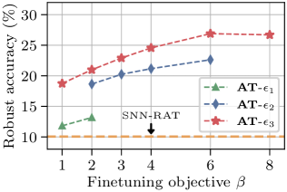
Figure 1: $\epsilon_{3}$-Robust accuracies under PGD²⁰ vs. $\beta$, with different baseline ANN standard AT perturbation levels.

used weaker (natural training) ANNs show minimal robustness under ensemble attacks (e.g., $\epsilon_{3}$-PGD²⁰ for CIFAR-10, Natural: 0.74, AT-$\epsilon_{1}$: 13.18, TRADES-$\epsilon_{1}$: 19.65, MART-$\epsilon_{1}$: 17.79, similar results can be observed with CIFAR-100 and SVHN). Here, conversion of a natural ANN with robust finetuning is analogous to the HIRE-SNN approach [45], where the finetuning objective and optimized parameters still differ, yet the final robustness remains weak.

Our finetuning objective and the use of trainable $V_{th}^{l}$ also appear critical to maintain robustness. We elaborate this later in our ablation studies in Suppl. B.3. In brief, we observed that natural $\operatorname{\mathcal{L}}_{\text{CE}}$ finetuning [27], or using fixed $V_{th}^{l}$ during robust finetuning, yields worse robustness (e.g., from Table B5, PGD²⁰ $\epsilon_{3}$-robustness when converting using natural $\operatorname{\mathcal{L}}_{\text{CE}}$: 10.03, using Eq. (9) but fixed $V_{th}^{l}$: 11.51, Ours: 13.18).

Fig. 1 shows the impact of baseline ANN training $\epsilon$, on the converted SNN, as well as the robustness-accuracy trade-off parameter in Eq. (9) for CIFAR-10. Note that we still perform finetuning with $\epsilon_{1}$ similar to [6], since larger perturbations via BPTT yields an unstable finetuning process. We observe that baseline ANN robustness transfers also in this case, and one can obtain even higher SNN robustness (e.g., $\epsilon_{3}$-robustness with AT-$\epsilon_{3}$, $\beta=6$: 26.90%) by using our method via heavier adversarial training of the ANN where optimization stability is not a problem.

5.2 Comparisons with State-of-the-Art Robust SNNs

In Table 2, we compare our approach with the current state-of-the-art method SNN-RAT, using the models and specifications from [6], under extensive white-box ensemble attacks. Our models yield both higher clean accuracy and adversarial robustness across various attacks, with some models being almost twice as robust against strong adversaries, e.g., clean/PGD⁴⁰ for CIFAR-10, SNN-RAT: 90.74/9.45, Ours (TRADES-$\epsilon_{1}$): 91.39/19.20. Note that in Table 2 we only compare our models trained through baseline ANNs with $\epsilon_{1}$-perturbations, since SNN-RAT also only uses $\epsilon_{1}$-adversaries (see Fig. 1 as to where SNN-RAT stands with respect to our models which can also exploit larger perturbation budgets via conversion). Overall, we observe that SNNs gradually get weaker against stronger adversaries, however our models maintain relatively higher robustness, also against powerful APGD${}_{\text{CE}}$ and T-APGD${}_{\text{CE}}$ attacks.

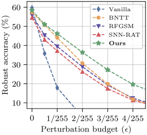
(a)

	Input Enc.	SNN Config.	Adv. Train	Clean Acc.	${\epsilon_{2}}$-Robust Acc.
					FGSM	PGD20
Vanilla	Direct	IF ($T=8$)	✗	57.29	1.93	0.13
RFGSM	Direct	IF ($T=8$)	✓	54.29	19.21	14.55
SNN-RAT	Direct	IF ($T=8$)	✓	52.76	22.39	16.63
Ours (AT-${\epsilon_{1}}$)	Direct	IF ($T=8$)	✓	55.98	22.91	17.82
Vanilla	Direct	LIF ($T=30$)	✗	59.62	1.76	0.05
BNTT	Poisson	LIF ($T=30$)	✗	57.33	17.64	11.88
RFGSM	Direct	LIF ($T=8$)	✓	55.92	17.51	12.42
SNN-RAT	Direct	LIF ($T=8$)	✓	54.47	19.66	11.37
Ours (AT-${\epsilon_{1}}$)	Direct	LIF ($T=8$)	✓	57.21	22.52	16.25
Ours (AT-${\epsilon_{1}}$)	Direct	LIF ($T=30$)	✓	58.36	24.02	19.67

(b)

Figure 2: Evaluations on TinyImageNet, with comparisons to SNN-RAT [6], an RFGSM based mixed AT baseline from [6], BNTT [19], and a vanilla SNN with natural training. SNNs with LIF neurons ($\tau=0.99$) use soft-reset as in [19]. In (a) we compare LIF-neuron models from the bottom half of the table in (b), using Ours with $T=30$.

Experiments on TinyImageNet: Results are summarized in Fig. 2. Here, we utilize the same VGG11 architecture used for BNTT [19], which has claimed robustness benefits through its batch-norm mechanism combined with Poisson input encoding (see Suppl. A.4 for attack details on this model). For comparisons, besides our usual IF ($T=8$) setting, we also converted (AT-$\epsilon_{1}$) ANNs by using LIF neurons ($\tau=0.99$) and soft-reset with direct coding.

Results in Fig. LABEL:fig:tinyb show that our model achieves a scalable, state-of-the-art solution for adversarially robust SNNs. Our model remains superior to RFGSM and SNN-RAT based end-to-end AT methods in the usual IF ($T=8$) setting with 17.82% robust accuracy. Results with LIF neurons show that our models can improve clean accuracy and robustness with higher $T$ ($T=30$), whereas RFGSM and SNN-RAT perform generally worse with LIF neurons. Results in Fig. LABEL:fig:tinya also reveal stronger robustness of our LIF-based ($T=30$) model starting from smaller perturbations, where it consistently outperforms existing methods. Our evaluations of BNTT show that AT is particularly useful for robustness (Ours ($T=30$): 19.67%, BNTT: 11.88%). Although direct coding does not approximate inputs and attacks become simpler [39], we show that direct coding SNNs can still yield higher resilience when adversarially calibrated.

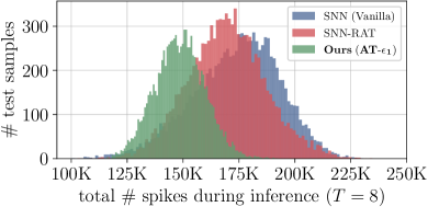
(a)

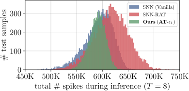
(b)

Figure 3: Coding efficiency comparisons of vanilla and adversarially robust SNNs.

5.3 Coding Efficiency of Adversarially Robust SNNs

In Fig. 3, we demonstrate higher coding efficiency of our approach. Specifically, VGG11 models consisted of 286,720 IF neurons operating for $T=8$ timesteps, which could induce a total of approx. 2.3M possible spikes for inference on a single sample. For CIFAR-10, on average for a test sample (i.e., mean of histograms in Fig. 3a), the total $\#$spikes elicited across a VGG11 was 148,490 with Ours, 169,566 for SNN-RAT, and 173,887 for a vanilla SNN. This indicates an average of only 6.47% active spiking neurons with our method, whereas SNN-RAT: 7.39%, and vanilla SNN: 7.58%. For CIFAR-100 in Fig. 3b, total $\#$spikes elicited on average was 589,774 with Ours, 616,439 for SNN-RAT, and 592,297 for vanilla SNN, across approx. 3.8M possible spikes from the 475,136 neurons in WRN-16-4. Here, our model was 15.52% actively spiking, whereas 16.22% with SNN-RAT. We did not observe an efficiency change with our more robust SNNs, and spike activity was similar to AT-$\epsilon_{1}$.

5.4 Further Experiments

Query-based Black-box Robustness: We evaluated SNNs with adversaries who have no knowledge of the defended model parameters, but can send a limited number of queries to it. Results are shown in Fig. 4, where our models consistently yield higher robustness (CIFAR-10 at 5000 queries: Ours: 50.2 vs. SNN-RAT: 46.3, CIFAR-100: 18.8 vs. 17.5). We also see that after 1000 queries, the baseline ANN shows weaker resilience than our SNNs. This reveals improved black-box robustness upon conversion to a spiking architecture, which is consistent with previous findings [9].

Transfer-based Black-box Robustness: Previous work [30] suggests that transfer-based attacks should be considered as a baseline to verify no potential influence of gradient masking or obfuscation. Accordingly, we present our evaluations in Suppl. B.1, where we verify (in Table B1) that fully black-box transfer attacks succeed less often than our ensemble white-box evaluations.

Performance of Ensemble Attacks: We elaborate the effectiveness of our ensemble attack approach in Suppl. B.2. In brief, we reveal that changing the shape or dampening magnitude of the surrogate gradient during BPTT can result in much stronger adversaries. We argue that our attacks reveal a more reliable robustness quantification for SNNs.

Out-of-distribution Generalization: We evaluated robust SNNs on CIFAR-10/100-C benchmarks [59] in Suppl. B.4. Our analyses yielded mean CIFAR-10-C accuracies of 83.85% with our model, whereas SNN-RAT: 81.72%, Vanilla SNN: 81.22% (CIFAR-100-C, Ours: 54.06%, SNN-RAT: 51.95%, Vanilla SNN: 46.14%). We observed that this result was consistent for all corruptions beyond noise [60] (see Tables B6 and B7).

6 Discussion

We propose an adversarially robust ANN-to-SNN conversion algorithm that exploits robustly trained baseline ANN weights at initialization, to improve SNN resiliency. Our method shows state-of-the-art robustness in feed-forward SNNs with low latency, outperforming recent end-to-end AT based methods in robustness, generalization, and coding efficiency. Our approach embraces any robust ANN training method to be incorporated in the domain of SNNs, and can also adopt further improvements to robustness, such as leveraging additional data [61]. Importantly, we empirically show that SNN evaluations against non-adaptive adversaries can be misleading [62], which has been the common practice in the field of SNNs.

We argue that direct AT methods developed for ANNs yield limited SNN robustness both because of their computational limitations with BPTT (e.g., use of single-step inner maximization), and also our findings with BPTT-based AT leading to SNNs with bias to the used surrogate gradient and vulnerability against adversaries that can leverage this. Therefore we propose to harness stronger and stable AT possibility through ANNs, and exploit better robustness gains.

Within the scope of this work we did not experiment with event-based data since (i) the adversarial attack problem in this setting needs to be tailored to the event-based domain where more specialized attacks are to be considered [41, 42, 43], and (ii) our method requires a robustly pre-trained ANN on the same task, and this is only possible with a specialized ANN that can process spatio-temporal data, e.g., [63]. Hence we instead focus on direct coding SNNs with low latency where conventional attacks remain powerful as an important open problem.

There were no observed white-box robustness benefits of SNNs with respect to ANNs. However, under black-box scenarios, our converted SNNs were more resilient. Overall, we achieved to significantly improve robustness of deep SNNs, considering their progress in safety-critical settings [3]. Since SNNs offer a promising energy-efficient technology, we argue that their robustness should be an important concern to be studied for reliable AI applications.

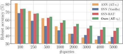
(a)

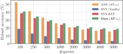
(b)

Figure 4: Square Attack [57] evaluations with limited number of queries for the baseline ANN with AT-$\epsilon_{1}$, end-to-end trained vanilla SNN, adversarially trained SNN-RAT, and our model (AT-$\epsilon_{1}$).

Appendix A Details on the Experimental Setup

A.1 Datasets and Models

We experimented with CIFAR-10, CIFAR-100, SVHN and TinyImageNet datasets. CIFAR-10 and CIFAR-100 datasets both consist of 50,000 training and 10,000 test images of resolution 32$\times$32, from 10 and 100 classes respectively [48]. SVHN dataset consists of 73,257 training and 26,032 test samples of resolution 32$\times$32 from 10 classes [49]. TinyImageNet dataset consists of 100,000 training and 10,000 test images of resolution 64$\times$64 from 200 classes [50]. We use VGG11 [51], ResNet-20 [52] and WideResNet [53] models with depth 16 and width 4 (i.e., WRN-16-4).

For baseline ANN optimization, we adopted the conventional data augmentation approaches that were found beneficial in robust adversarial training [61, 64]. During SNN finetuning after conversion, we follow the simple traditional data augmentation scheme that was also adopted in previous work [6]. This procedure involves randomly cropping images into 32$\times$32 dimensions by padding zeros for at most 4 pixels around it, and randomly performing a horizontal flip. For TinyImageNet we instead perform a random resized crop to 64$\times$64, also followed by a random horizontal flip. All image pixel values are normalized using the conventional metrics estimated on the training set of each dataset.

A.2 Robust Training Configurations

Baseline ANNs: During robust optimization with standard AT, TRADES, and MART, adversarial examples are iteratively crafted for each mini-batch (inner maximization step of Eq. (4)), by using 10 PGD steps with random starts under $l_{\infty}$-bounded perturbations, and $\eta=2.5\times\epsilon/\#$steps. For standard AT and MART we perform the inner maximization PGD using $\operatorname{\mathcal{L}}_{\text{PGD}}=\operatorname{\mathcal{L}}_{\text{CE}}(f_{\operatorname{\bm{\theta}}}(\operatorname{\mathbf{\tilde{x}}}),y)$, whereas for TRADES we use $\operatorname{\mathcal{L}}_{\text{PGD}}=D_{\text{KL}}(f_{\operatorname{\bm{\theta}}}(\operatorname{\mathbf{\tilde{x}}})||f_{\operatorname{\bm{\theta}}}(\operatorname{\mathbf{x}}))$ as the inner maximization loss, following the original works [8, 35, 36]. We set the trade-off parameter $\lambda_{\text{MART}}=4$ in all experiments, and $\lambda_{\text{TRADES}}=6$ in CIFAR-10 and $\lambda_{\text{TRADES}}=3$ in CIFAR-100 and SVHN experiments. We present extended robustness evaluations of the baseline ANNs used in our experiments in Table A1.

Converted SNNs: During initialization of layer-wise firing thresholds, we use 10 training mini-batches of size 64 with a calibration sequence length of $T_{c}=100$ timesteps, and observe the pre-activation values. We choose the maximum value in the $\rho=99.7\%$ percentile of the distribution of observed values. This process is performed similarly to [27, 47], and is a better alternative to simply using the largest observed pre-activation value for threshold balancing [23], since the procedure involves the use of randomly sampled training batches which might lead to large valued outliers compared to the rest of the distribution. We use $\kappa=0.3$ in CIFAR-10 and SVHN, and $\kappa=0.1$ in CIFAR-100 and TinyImageNet experiments. During BPTT-based finetuning, we used the piecewise linear surrogate gradient in Eq (16) with $\gamma_{w}=1$, as in [6]. For the initial random step of RFGSM, we set $\alpha=\epsilon_{1}/2$ in CIFAR-10 and SVHN, and $\alpha=\epsilon_{1}/5$ in CIFAR-100 and TinyImageNet experiments. For CIFAR-10 experiments with AT-$\epsilon_{2}$ and AT-$\epsilon_{3}$, we used $\alpha=\epsilon/4$.

End-to-end trained SNNs used for comparisons were initialized statically at $V_{th}^{l}=1$ for all layers, as in [6]. During robust finetuning, we impose a lower bound for the trainable firing thresholds such that they remain $V_{th}^{l}\geq 0.03$. At inference-time with our models, for tdBN layers, we use the mean and variance moving averages estimated during the robust finetuning process from scratch. Since we performed conversion with baseline ANNs without bias terms [23, 65], only in CIFAR-10/100 experiments we introduce bias terms during finetuning in the output dense layers to be also optimized, in order to have identical networks to SNN-RAT. Although it slightly increased model performance, we did not find the use of bias terms strictly necessary in our method.

Table A1: Robustness evaluations (%) of used baseline ANN architectures in our experiments. All attacks are evaluated under an $l_{\infty}$-norm bounded $\epsilon_{3}=8/255$ perturbation budget. AA_∞ indicates AutoAttack evaluations. PGD attack step sizes were determined by $2.5\times\epsilon/\#$steps. Maximum number of queries for SquareAttack were set to 5000.

		Clean Acc.	$\epsilon_{3}$-Robust Accuracies
			FGSM	PGD10	PGD50	APGD${}_{\text{CE}}$	Square	AA∞
CIFAR-10 with VGG11	Natural	95.10	20.35	0.13	0.06	1.07	0.45	0.00
	AT-${\epsilon_{1}}$	93.55	42.71	21.86	20.76	18.98	32.99	16.64
	TRADES-${\epsilon_{1}}$	92.10	51.26	33.59	32.56	29.75	41.90	27.62
	MART-${\epsilon_{1}}$	92.68	47.21	28.43	27.43	24.58	37.56	21.98
	AT-${\epsilon_{2}}$	91.05	51.55	37.00	36.32	34.62	45.87	32.61
	AT-${\epsilon_{3}}$	85.07	58.30	53.57	53.24	51.65	52.98	45.05
CIFAR-100 with WRN-16-4	Natural	78.93	6.79	0.00	0.00	0.00	0.00	0.00
	AT-${\epsilon_{1}}$	74.90	20.23	9.85	9.34	8.49	15.53	7.05
	TRADES-${\epsilon_{1}}$	73.87	20.40	11.07	10.53	9.64	15.61	8.43
	MART-${\epsilon_{1}}$	72.61	23.93	15.08	14.47	13.26	19.51	11.04
SVHN with ResNet-20	Natural	97.08	63.83	0.71	0.08	1.87	1.38	0.08
	AT-${\epsilon_{1}}$	96.50	52.53	30.36	29.25	25.86	29.30	23.58
	TRADES-${\epsilon_{1}}$	96.29	54.11	33.43	32.18	29.13	32.10	27.16
	MART-${\epsilon_{1}}$	96.16	56.66	36.02	34.82	31.04	31.70	27.65

Optimization: We used momentum SGD with a cosine annealing based learning rate scheduler, and a batch size of 64 in all model training settings. All end-to-end trained models (i.e., baseline ANNs and vanilla SNNs) were optimized for 200 epochs with an initial learning rate of 0.1, following the conventional settings [8, 35, 36]. After ANN-to-SNN conversion and setting initial thresholds, SNNs were finetuned for 60 epochs on CIFAR-10, SVHN and TinyImageNet, and 80 epochs on CIFAR-100, with an initial learning rate of 0.001. During robust finetuning, we used a weight decay parameter of 0.001 in CIFAR-10, SVHN and TinyImageNet experiments, whereas we used 0.0001 for CIFAR-100. We also used lower weight decay parameters of 0.0005 and 0.0001 during post-conversion finetuning of AT-$\epsilon_{2}$ and AT-$\epsilon_{3}$ models respectively in our CIFAR-10 experiments.

Computational Overhead: Although our method uses a larger amount of total training epochs (baseline ANN training and robust SNN finetuning), the overhead does not differ much from end-to-end AT methods (e.g., SNN-RAT) due to the heavier computational load of AT with SNNs which involves the temporal dimension. To illustrate quantitatively (CIFAR-10 with VGG11), Ours: baseline ANN training for 200 epochs takes $\sim$11 hours and robust SNN finetuning for 60 epochs takes $\sim$10.5 hours, SNN-RAT: robust end-to-end training for 200 epochs takes $\sim$23 hours wall-clock time.

Implementations: All models were implemented with the PyTorch 1.13.0 [66] library, and experiments were performed using GPU hardware of types NVIDIA A40, NVIDIA Quadro RTX 8000 and NVIDIA Quadro P6000. Adversarial attacks were implemented using the TorchAttacks [67] library, with the default attack hyper-parameters. Our code and implementations can be found at: https://github.com/IGITUGraz/RobustSNNConversion.

A.3 Robust SNN Finetuning Parameter Updates with Surrogate Gradients

Our robust optimization objective after the initial ANN-to-SNN conversion step follows:

$$\min_{\operatorname{\bm{\theta}}}\,\operatorname{\mathbb{E}}\left[\operatorname{\mathcal{L}}_{\text{CE}}(f_{\operatorname{\bm{\theta}}}(\operatorname{\mathbf{x}}),y)+\beta\cdot\max_{\operatorname{\mathbf{\tilde{x}}}\in\Delta_{\epsilon}^{p}(\operatorname{\mathbf{x}})}D_{\text{KL}}(f_{\operatorname{\bm{\theta}}}(\operatorname{\mathbf{\tilde{x}}})||f_{\operatorname{\bm{\theta}}}(\operatorname{\mathbf{x}}))\right],$$ (11)

where $\operatorname{\bm{\theta}}$ consist of $\{\operatorname{\mathbf{W}}^{l},\varphi^{l},\omega^{l}\}_{l=1}^{L}$ and $\{V_{th}^{l}\}_{l=1}^{L-1}$, the adversarial example $\operatorname{\mathbf{\tilde{x}}}\in\Delta_{\epsilon}^{\infty}(\operatorname{\mathbf{x}})$ is obtained at the inner maximization via RFGSM using $\mathcal{L}_{\text{RFGSM}}=D_{\text{KL}}(f_{\operatorname{\bm{\theta}}}(\operatorname{\mathbf{x}}^{\prime})||f_{\operatorname{\bm{\theta}}}(\operatorname{\mathbf{x}}))$,

$$\begin{split}\operatorname{\mathcal{L}}_{\text{CE}}=-\sum_{j}y^{(j)}\log(f_{\operatorname{\bm{\theta}}}^{(j)}(\operatorname{\mathbf{x}}))\quad\text{and}\quad D_{\text{KL}}=\sum_{j}f_{\operatorname{\bm{\theta}}}^{(j)}(\operatorname{\mathbf{\tilde{x}}})\log\frac{f_{\operatorname{\bm{\theta}}}^{(j)}(\operatorname{\mathbf{\tilde{x}}})}{f_{\operatorname{\bm{\theta}}}^{(j)}(\operatorname{\mathbf{x}})}.\end{split}$$ (12)

Following the robust optimization objective that minimizes an overall loss function expressed in the brackets of Eq. (11), say $\operatorname{\mathcal{L}}_{\text{robust}}$, the gradient-based synaptic connectivity weight and firing threshold updates in the hidden layers of the SNN $l=\{1,\ldots,L-1\}$ are determined via BPTT as:

$$\Delta\operatorname{\mathbf{W}}^{l}=\sum_{t}\frac{\partial\operatorname{\mathcal{L}}_{\text{robust}}}{\partial\operatorname{\mathbf{W}}^{l}}=\sum_{t}\frac{\partial\operatorname{\mathcal{L}}_{\text{robust}}}{\partial\operatorname{\mathbf{s}}^{l}(t)}\frac{\partial\operatorname{\mathbf{s}}^{l}(t)}{\partial\operatorname{\mathbf{z}}^{l}(t)}\frac{\partial\operatorname{\mathbf{z}}^{l}(t)}{\partial\operatorname{\mathbf{v}}^{l}(t^{-})}\frac{\partial\operatorname{\mathbf{v}}^{l}(t^{-})}{\partial\operatorname{\mathbf{W}}^{l}},$$ (13)

$$\Delta V_{th}^{l}=\sum_{t}\frac{\partial\operatorname{\mathcal{L}}_{\text{robust}}}{\partial V_{th}^{l}}=\sum_{t}\frac{\partial\operatorname{\mathcal{L}}_{\text{robust}}}{\partial\operatorname{\mathbf{s}}^{l}(t)}\frac{\partial\operatorname{\mathbf{s}}^{l}(t)}{\partial\operatorname{\mathbf{z}}^{l}(t)}\frac{\partial\operatorname{\mathbf{z}}^{l}(t)}{\partial V_{th}^{l}},$$ (14)

where $\operatorname{\mathbf{z}}^{l}(t)=\operatorname{\mathbf{v}}^{l}(t^{-})-V_{th}^{l}$ is the input to the Heaviside step function: $\operatorname{\mathbf{s}}^{l}(t)=H(\operatorname{\mathbf{z}}^{l}(t))$. For BPTT we use the piecewise linear surrogate gradient with a unit dampening factor:

$$\frac{\partial\operatorname{\mathbf{s}}^{l}(t)}{\partial\operatorname{\mathbf{z}}^{l}(t)}\vcentcolon=\max\{0,1-|\operatorname{\mathbf{z}}^{l}(t)|\}.$$ (15)

Remaining gradient terms can be computed via LIF neuron dynamics. For the layers containing tdBN operations, the parameters $\varphi^{l}$ and $\omega^{l}$ are also updated similarly through normalized $\hat{\operatorname{\mathbf{s}}}^{l}(t)$, following the original gradient computations from [68], which are however gathered temporally [20]. Since there is no spiking activity in the output layer, weight updates can be computed via BPTT without surrogate gradients, similar to the definitions from [45, 27]. Our complete robust ANN-to-SNN conversion procedure is outlined in Algorithm 1.

Algorithm 1 Adversarially robust ANN-to-SNN conversion

1:Input: Training dataset $\operatorname{\mathcal{D}}$, adversarially pre-trained baseline ANN parameters $\{\operatorname{\mathbf{W}}^{l},\varphi^{l},\omega^{l}\}_{l=1}^{L}$, number of calibration samples, calibration sequence length $T_{c}$, percentile $\rho$, threshold scaling factor $\kappa$, number of finetuning iterations, perturbation strength $\epsilon$ and random step $\alpha$ for RFGSM, simulation timesteps $T$, membrane leak factor $\tau$, trade-off parameter $\beta$.

2:Output: Robust SNN $f$ with parameters $\operatorname{\bm{\theta}}$ consisting of $\{\operatorname{\mathbf{W}}^{l},\varphi^{l},\omega^{l}\}_{l=1}^{L}$ and $\{V_{th}^{l}\}_{l=1}^{L-1}$.

3:$\triangleright$ Converting the adversarially trained baseline ANN

4:Initialize: Set weights of the SNN $f$ directly from the pre-trained ANN parameters $\{\operatorname{\mathbf{W}}^{l},\varphi^{l},\omega^{l}\}_{l=1}^{L}$.

5:for $l=1$ to $L-1$ do

6:   for $c=1$ to $\#calibration\_samples$ do

7:      for $t=1$ to $T_{c}$ do

8:         $\mathbf{r}^{l}\leftarrow$ Store pre-activation values at layer $l$ during forward pass with direct input coding.

9:      end for

10:      if max$[\rho$-percentile of the dist. in $\mathbf{r}^{l}]>V^{l}_{th}$ then

11:         $V^{l}_{th}=\text{max}[\rho$-percentile of the distribution in $\mathbf{r}^{l}]$

12:      end if

13:   end for

14:end for

15:$\triangleright$ Initializing trainable firing thresholds

16:for $l=1$ to $L-1$ do

17:   $V^{l}_{th}\leftarrow\kappa\cdot V^{l}_{th}$

18:end for

19:$\triangleright$ Robust finetuning of SNN after conversion

20:for $i=1$ to $\#finetuning\_iterations$ do

21:   Sample a mini-batch of $(\operatorname{\mathbf{x}},y)\sim\operatorname{\mathcal{D}}$

22:$\quad\triangleright$ Inner maximization for single-step adversarial examples

23:   $\operatorname{\mathbf{x}}^{\prime}\leftarrow\operatorname{\mathbf{x}}+\,\alpha\cdot\text{sign}\left(\mathcal{N}(\mathbf{0},\mathbf{I})\right)$

24:   $f_{\operatorname{\bm{\theta}}}(\operatorname{\mathbf{x}}^{\prime}),f_{\operatorname{\bm{\theta}}}(\operatorname{\mathbf{x}})\leftarrow$ Forward pass direct coded $\operatorname{\mathbf{x}}^{\prime}$ and $\operatorname{\mathbf{x}}$ via Eqs. (1), (2), (3), (7), with $\tau$.

25:   $\operatorname{\mathbf{\tilde{x}}}\leftarrow\operatorname{\mathbf{x}}^{\prime}+\,(\epsilon-\alpha)\cdot\text{sign}\left(\nabla_{\operatorname{\mathbf{x}}^{\prime}}\mathcal{L}_{\text{RFGSM}}\right)$ with $\mathcal{L}_{\text{RFGSM}}=D_{\text{KL}}(f_{\operatorname{\bm{\theta}}}(\operatorname{\mathbf{x}}^{\prime})||f_{\operatorname{\bm{\theta}}}(\operatorname{\mathbf{x}}))$.

26:$\quad\triangleright$ Outer optimization with the robust finetuning objective

27:   $f_{\operatorname{\bm{\theta}}}(\operatorname{\mathbf{x}}),f_{\operatorname{\bm{\theta}}}(\operatorname{\mathbf{\tilde{x}}})\leftarrow$ Forward pass direct coded $\operatorname{\mathbf{x}}$ and $\operatorname{\mathbf{\tilde{x}}}$ via Eqs. (1), (2), (3), (7), with $\tau$.

28:   $\operatorname{\mathcal{L}}_{\text{robust}}\leftarrow\operatorname{\mathbb{E}}\left[\operatorname{\mathcal{L}}_{\text{CE}}(f_{\operatorname{\bm{\theta}}}(\operatorname{\mathbf{x}}),y)+\beta\cdot D_{\text{KL}}\left(f_{\operatorname{\bm{\theta}}}(\operatorname{\mathbf{\tilde{x}}})||f_{\operatorname{\bm{\theta}}}(\operatorname{\mathbf{x}})\right)\right]$

29:   $\Delta\operatorname{\mathbf{W}}^{l}\leftarrow\sum_{t}\frac{\partial\operatorname{\mathcal{L}}_{\text{robust}}}{\partial\operatorname{\mathbf{W}}^{l}}$

30:   $\Delta\varphi^{l}\leftarrow\sum_{t}\frac{\partial\operatorname{\mathcal{L}}_{\text{robust}}}{\partial\varphi^{l}}$

31:   $\Delta\omega^{l}\leftarrow\sum_{t}\frac{\partial\operatorname{\mathcal{L}}_{\text{robust}}}{\partial\omega^{l}}$

32:   $\Delta V_{th}^{l}\leftarrow\sum_{t}\frac{\partial\operatorname{\mathcal{L}}_{\text{robust}}}{\partial V_{th}^{l}}$

33:end for

A.4 Ensemble Adversarial Attacks

The success of an SNN attack depends critically on the surrogate gradient used for by the adversary. Therefore we consider adaptive adversaries that perform a number of attacks for any test sample, where the surrogate gradient used to approximate the discontinuity of the spike function during BPTT varies in each case. Specifically, as part of the attack ensemble we perform backpropagation by using the piecewise linear (triangular) function [15, 14] defined as in Eq. (16) with $\gamma_{w}\in\{0.25,0.5,1.0,2.0,3.0\}$,

$$\frac{\partial\operatorname{\mathbf{s}}^{l}(t)}{\partial\operatorname{\mathbf{z}}^{l}(t)}\vcentcolon=\frac{1}{\gamma_{w}^{2}}\cdot\max\{0,\gamma_{w}-|\operatorname{\mathbf{z}}^{l}(t)|\},$$ (16)

the exponential surrogate gradient function [16] defined as in Eq. (17) with hyper-parameters $(\gamma_{d},\gamma_{s})\in\{(0.3,0.5),(0.3,1.0),(0.3,2.0),(1.0,0.5),$ $(1.0,1.0),(1.0,2.0)\}$,

$$\frac{\partial\operatorname{\mathbf{s}}^{l}(t)}{\partial\operatorname{\mathbf{z}}^{l}(t)}\vcentcolon=\gamma_{d}\cdot\exp{\left(-\gamma_{s}\cdot|\operatorname{\mathbf{z}}^{l}(t)|\right)},$$ (17)

and the rectangular function [11] defined as in Eq. (18) with $\gamma_{w}\in\{0.25,0.5,1.0,2.0,4.0\}$,

$$\frac{\partial\operatorname{\mathbf{s}}^{l}(t)}{\partial\operatorname{\mathbf{z}}^{l}(t)}\vcentcolon=\frac{1}{\gamma_{w}}\cdot\text{sign}\left(|\operatorname{\mathbf{z}}^{l}(t)|<\frac{\gamma_{w}}{2}\right).$$ (18)

For the rectangular and piecewise linear (triangular) functions, $\gamma_{w}$ indicates the width that determines the input range to activate the gradient. The dampening factor of these surrogate gradients is then inversely proportional to $\gamma_{w}$ [6, 69, 11, 12]. For the exponential function, $\gamma_{d}$ controls the dampening and $\gamma_{s}$ controls the steepness. A conventional choice for the exponential is $(\gamma_{d},\gamma_{s})=(0.3,1.0)$ [16], while we also experimented by varying these parameters. Interestingly, we could verify that varying the shape and parameters of this surrogate gradient function occasionally had an impact on the success of the adversary for various test samples. This scenario, for instance, indicates having approximate gradient information long before the membrane potential reaches the firing threshold (i.e., larger $\gamma_{w}$), which can be useful to attack SNNs from the perspective of an adaptive adversary. In Section B.2 we present the effectiveness of the individual components of the ensemble.

In the ensemble, we also considered the straight-through estimator (STE) [70], backward pass through rate (BPTR) [6], and a conversion-based approximation, where spiking neurons are replaced with ReLU functions during BPTT [6]. STE uses an identity function as the surrogate gradient for all SNN neurons during backpropagation. BPTR performs a differentiable approximation by taking the derivative of the spike functions directly from the average firing rate of the neurons between layers [6]. In this case the gradient does not accumulate through time, and the complete neuronal dynamic is approximated during backpropagation by a single STE that maintains gradients for neurons that have a non-zero spike rate in the forward pass. We use the same BPTR implementation based on the evaluations from [6]. Conversion-based approximation was an earlier attempt to design adversarial attacks on SNNs which we also include, although we found it to be only minimally effective [5].

Attacks on the Poisson encoding BNTT model: In our TinyImageNet experiments, for FGSM and PGD²⁰ on the BNTT model [19], we used the SNN-crafted BPTT-based adversarial input generation methodology by [9]. These attacks approximate the non-differentiable Poisson input encoding layer by using the gradients obtained for the first convolution layer activations during the attack, and was found to be a powerful substitute. We also used two expectation-over-transformation (EOT) iterations [71] while crafting adversarial examples on this model, due to the involved randomness in input encoding [30]. Overall, we use the same surrogate gradient ensemble approach, however with an obligatory approximation of the input encoding and EOT iterations for stable gradient estimates.

Appendix B Additional Experiments

B.1 Black-box Transfer Attacks

In Table B1 we present our transfer-based black-box robustness evaluations [58], using both the baseline ANN, and a similar SNN model obtained with the same conversion procedure using a different random seed. We craft adversarial examples on the source models with PGD²⁰ also in an ensemble setting. In all models, we observe that white-box robust accuracies are significantly lower than black-box cases. This result holds both for the $\epsilon_{1}$ perturbation budget where the models were trained and finetuned on, as well as $\epsilon_{3}$ where we investigate robust generalization to higher perturbation bounds. Only in CIFAR-10, we observed that adversarially trained baseline ANNs used for conversion were able to craft stronger adversarial examples than the SNNs converted and finetuned in an identical setting (e.g., $\epsilon_{3}$-robustness for AT-$\epsilon_{1}$: BB${}_{\text{ANN}}$: 29.81%, BB${}_{\text{SNN}}$: 42.27%). We believe that this is related to our weaker choice of $\beta=2$ for finetuning in CIFAR-10 experiments, whereas we used $\beta=4$ in all other models. On another note, we observed that BB${}_{\text{SNN}}$ attacks are highly powerful on converted SNNs based on natural baseline ANN training (e.g., for CIFAR-10 $\epsilon_{3}$-robustness WB: 0.74%, BB${}_{\text{SNN}}$: 6.87%), demonstrating their weakness even in the black-box setting.

Table B1: Evaluating $\epsilon_{1}=2/255$ and $\epsilon_{3}=8/255$ robust accuracies under black-box (BB) transfer attacks [58], obtained via adversarial examples crafted with ensemble PGD²⁰ attacks on a source model. In white-box (WB) setting, the source and target models are identical. BB${}_{\text{SNN}}$ indicates attacks via a source model that undergoes the same ANN-to-SNN conversion procedure as the target model, with a different random seed during finetuning. BB${}_{\text{ANN}}$ indicates transfer attacks where the source model is the baseline ANN used for conversion (hence no ensemble needed).

			Adversarially Robust ANN-to-SNN Conversion
		Clean Acc.	$\epsilon_{1}$-Robust Accuracies			$\epsilon_{3}$-Robust Accuracies
			WB	BB${}_{\text{SNN}}$	BB${}_{\text{ANN}}$	WB	BB${}_{\text{SNN}}$	BB${}_{\text{ANN}}$
CIFAR-10 with VGG11	Natural	93.53	59.22	76.93	82.21	0.74	6.87	21.99
	AT-${\epsilon_{1}}$	92.14	70.02	85.40	82.04	13.18	42.27	29.81
	TRADES-${\epsilon_{1}}$	91.39	72.00	86.21	82.29	19.65	52.34	38.18
	MART-${\epsilon_{1}}$	91.47	70.35	84.19	81.43	17.79	41.82	32.26
CIFAR-100 with WRN-16-4	Natural	70.87	35.49	45.95	64.44	1.40	3.15	48.12
	AT-${\epsilon_{1}}$	70.02	44.73	54.88	59.36	7.64	11.88	25.52
	TRADES-${\epsilon_{1}}$	67.84	42.73	53.14	58.20	7.79	11.86	27.23
	MART-${\epsilon_{1}}$	67.10	43.46	53.21	57.83	8.90	13.39	28.03
SVHN with ResNet-20	Natural	94.18	74.30	82.21	91.71	10.35	14.96	89.18
	AT-${\epsilon_{1}}$	91.90	71.80	81.47	84.18	21.51	29.94	44.51
	TRADES-${\epsilon_{1}}$	92.78	74.27	83.30	85.00	23.96	31.62	43.37
	MART-${\epsilon_{1}}$	92.71	74.82	82.94	85.67	24.11	33.01	44.27

On the Analysis of Gradient Obfuscation: Previous SNN robustness studies [45, 6] analyzes gradient obfuscation [30] solely based on the five principles: (1) iterative attacks should perform better than single-step attacks, (2) white-box attacks should perform better than transfer-based attacks, (3) increasing attack perturbation bound should result in lower robust accuracies, (4) unbounded attacks can nearly reach 100% success, (5) adversarial examples can not be found through random sampling. In the main paper and our results presented here, we could confirm all of these observations in our evaluations. However, we argue that more reliable SNN assessments should ideally go beyond these, as we clarify in further depth via our evaluations with adaptive adversaries [10].

Table B2: Evaluating $\epsilon_{3}=8/255$ FGSM attack robust accuracies from our CIFAR-10 experiments with VGG11, under individual components of the white-box ensemble. Triangular (piecewise linear), exponential and rectangular surrogate gradients were used as part of BPTT. Underlined values indicate the strongest individual attack within the ensemble.

		SNN- RAT [6]	ANN-to-SNN Conversion (Ours)
			Natural	AT-${\epsilon_{1}}$	TRADES-${\epsilon_{1}}$	MART-${\epsilon_{1}}$
Clean Accuracy		90.74	93.53	92.14	91.39	91.47
Ensemble FGSM		32.80	15.71	33.94	41.42	44.39
Triangular	$\gamma_{w}=1.0$	45.01	28.16	53.61	71.50	62.16
	$\gamma_{w}=2.0$	39.27	63.06	74.36	82.94	79.27
	$\gamma_{w}=3.0$	43.23	77.79	83.59	87.72	86.30
	$\gamma_{w}=0.5$	82.20	19.62	39.25	52.09	51.56
	$\gamma_{w}=0.25$	90.15	54.15	57.48	51.03	50.16
Exponential	$(\gamma_{d},\gamma_{s})=(0.3,0.5)$	48.94	80.75	83.89	87.68	86.70
	$(\gamma_{d},\gamma_{s})=(0.3,1.0)$	36.91	54.96	69.65	79.66	74.97
	$(\gamma_{d},\gamma_{s})=(0.3,2.0)$	37.65	27.15	51.66	67.60	60.02
	$(\gamma_{d},\gamma_{s})=(1.0,0.5)$	62.73	89.41	89.01	90.36	89.41
	$(\gamma_{d},\gamma_{s})=(1.0,1.0)$	41.63	64.45	75.37	83.30	79.34
	$(\gamma_{d},\gamma_{s})=(1.0,2.0)$	38.65	32.07	55.96	70.99	62.55
Rectangular	$\gamma_{w}=0.25$	90.01	88.14	85.22	71.08	66.57
	$\gamma_{w}=0.5$	89.15	26.58	42.51	51.18	53.44
	$\gamma_{w}=1.0$	65.28	25.10	49.85	68.98	61.68
	$\gamma_{w}=2.0$	45.21	63.45	73.59	83.49	80.22
	$\gamma_{w}=4.0$	52.62	88.84	89.42	90.93	89.43
Backward Pass Through Rate		51.46	23.90	41.33	46.68	58.26
Conversion-based Approx.		84.25	39.73	55.35	89.43	87.79
Straight-Through Estimation		90.14	92.84	90.74	90.68	91.03

B.2 Evaluations with Alternative Surrogate Gradient Functions

Our detailed results for one particular ensemble attack is demonstrated in Table B2, where we focus on single-step FGSM without an initial randomized start. The third row indicates a naive BPTT-based FGSM attack where the adversary uses the same surrogate gradient function utilized during model training (e.g., SNN-RAT: 45.01%, Ours (AT-$\epsilon_{1}$): 53.61%). Importantly, we observe that there are stronger attacks that can be crafted by a versatile adversary,

Table B3: Impact of ensemble SNN attacks on CIFAR-10, with comparisons to ANNs under the analogous $\epsilon_{3}$-attack. PGD${}^{20}_{\text{vanilla}}$ uses BPTT with training-time surrogate gradient.

CIFAR-10 with VGG11	ANN		SNN
	Clean	PGD20	Clean	PGD${}^{20}_{\text{vanilla}}$	PGD${}^{20}_{\text{ensemble}}$
AT-${\epsilon_{1}}$	93.55	21.15	92.14	37.42	13.18
TRADES-${\epsilon_{1}}$	92.10	32.94	91.39	62.03	19.65
MART-${\epsilon_{1}}$	92.68	27.54	91.47	49.90	17.79

by varying the shape or parameters of the used surrogate gradient. Moreover, in this particular case with FGSM attacks, we observe 4-6$\%$ difference in attack performance between the strongest individual attack configuration within the ensemble (e.g., underlined SNN-RAT: 36.91%, Ours (AT-$\epsilon_{1}$): 39.25%), versus using an ensemble of alternative possibilities (e.g., SNN-RAT: 32.80%, Ours (AT-$\epsilon_{1}$): 33.94%). This further emphasizes the relative strength of our evaluations, in comparison to traditional naive settings.

Table B4: Impact of ensemble SNN attacks on CIFAR-100, with comparisons to ANNs under the analogous $\epsilon_{3}$-attack. PGD${}^{20}_{\text{vanilla}}$ uses BPTT with training-time surrogate gradient.

CIFAR-100 with WRN-16-4	ANN		SNN
	Clean	PGD20	Clean	PGD${}^{20}_{\text{vanilla}}$	PGD${}^{20}_{\text{ensemble}}$
AT-${\epsilon_{1}}$	74.90	9.46	70.02	12.56	7.64
TRADES-${\epsilon_{1}}$	73.87	10.74	67.84	12.97	7.79
MART-${\epsilon_{1}}$	72.61	14.72	67.10	14.27	8.90

Tables B3 and B4 show a comparison of ANNs and SNNs under analogous PGD²⁰ attack settings. Here, SNN evaluations under PGD${}^{20}_{\text{vanilla}}$ indicate naive BPTT-based attacks, where the adversary only uses the same surrogate gradient utilized during training. Simply running these evaluations would generally be considered analogous to those for the PGD²⁰ ANN attacks [6], although they are essentially not identical. Considering PGD${}^{20}_{\text{vanilla}}$ accuracies, results might even be (wrongly) perceived as SNNs being more robust than ANNs, as claimed in previous work based on shallow models and naive evaluation settings [72, 73]. However, since the SNN attack depends on the surrogate gradient, we also consider the ensemble PGD²⁰, as we did throughout our work. This stronger attack is not necessarily equivalent to the ANN attack either, but we believe it is a better basis for comparison.

B.3 Ablations on the Robust SNN Finetuning Objective

Our ablation studies are presented in Table B5. The first three rows respectively denote comparisons to end-to-end trained SNNs using a natural cross-entropy loss, and using our robust finetuning objective without and with trainable thresholds, for 200 epochs. Note that with the model in the third row, we are essentially comparing our hybrid ANN-to-SNN conversion approach, to simply end-to-end adversarially training the SNN using the TRADES objective. Our method yields approximately twice as more robust models than the model in the third row (i.e., ensemble APGD${}_{\text{CE}}$: 4.72 versus 10.05), indicating that the weight initialization from an adversarially trained ANN brings significant gains. The fourth model, as included in the main manuscript, indicates weight initialization from a naturally trained ANN within our conversion approach, which yields nearly no robustness since these initial weights are inclined to a non-robust local minimum solution during natural ANN training.

Remaining models compare different choices for $\mathcal{L}_{\text{RFGSM}}$ (e.g., adversarial cross-entropy loss [32]), and the outer optimization scheme (e.g., standard AT [8]), which we have eventually chosen to follow a similar one to TRADES [35]. We also observed significant robustness benefits of using trainable $V_{th}^{l}$ during post-conversion finetuning as proposed in [27] (e.g., clean/PGD²⁰: 91.09/9.39 vs. 92.14/10.05). Overall, these results show that our design choices were important to achieve better robustness. Nevertheless, several alternatives in Table B5 (e.g., standard AT based outer optimization or $\operatorname{\mathcal{L}}_{\text{CE}}(f_{\operatorname{\bm{\theta}}}(\operatorname{\mathbf{x}}^{\prime}),y)$ based RFGSM) still remained effective to outperform existing defenses.

Table B5: Ablations for the robust SNN finetuning objective with our CIFAR-10 experiments. Robust accuracies are evaluated via ensemble white-box attacks. Bottom row indicates our method.

Baseline ANN	Inner Max. $\mathcal{L}_{\text{RFGSM}}$	Outer Optimization	Trainable $V_{th}^{l}$	Clean Acc.	$\epsilon_{3}$-Robust Accuracies
					FGSM	PGD20	APGD${}_{\text{CE}}$
✗	$-$	$\operatorname{\mathcal{L}}_{\text{CE}}(f_{\operatorname{\bm{\theta}}}(\operatorname{\mathbf{x}}),y)$	✗	93.73	6.43	0.00	0.00
✗	$D_{\text{KL}}(f_{\operatorname{\bm{\theta}}}(\operatorname{\mathbf{x}}^{\prime})||f_{\operatorname{\bm{\theta}}}(\operatorname{\mathbf{x}}))$	Eq. (11)	✗	91.90	24.94	7.23	5.32
✗	$D_{\text{KL}}(f_{\operatorname{\bm{\theta}}}(\operatorname{\mathbf{x}}^{\prime})||f_{\operatorname{\bm{\theta}}}(\operatorname{\mathbf{x}}))$	Eq. (11)	✓	91.75	23.83	6.70	4.72
Natural	$D_{\text{KL}}(f_{\operatorname{\bm{\theta}}}(\operatorname{\mathbf{x}}^{\prime})||f_{\operatorname{\bm{\theta}}}(\operatorname{\mathbf{x}}))$	Eq. (11)	✓	93.53	15.71	0.74	0.44
AT-$\epsilon_{1}$	$-$	$\operatorname{\mathcal{L}}_{\text{CE}}(f_{\operatorname{\bm{\theta}}}(\operatorname{\mathbf{x}}),y)$	✓	92.18	32.31	10.03	8.40
AT-$\epsilon_{1}$	$\operatorname{\mathcal{L}}_{\text{CE}}(f_{\operatorname{\bm{\theta}}}(\operatorname{\mathbf{x}}^{\prime}),y)$	$\operatorname{\mathcal{L}}_{\text{CE}}(f_{\operatorname{\bm{\theta}}}(\operatorname{\mathbf{\tilde{x}}}),y)$	✓	92.02	34.17	12.19	9.40
AT-$\epsilon_{1}$	$D_{\text{KL}}(f_{\operatorname{\bm{\theta}}}(\operatorname{\mathbf{x}}^{\prime})||f_{\operatorname{\bm{\theta}}}(\operatorname{\mathbf{x}}))$	$\operatorname{\mathcal{L}}_{\text{CE}}(f_{\operatorname{\bm{\theta}}}(\operatorname{\mathbf{\tilde{x}}}),y)$	✓	91.59	32.83	11.78	9.26
AT-$\epsilon_{1}$	$\operatorname{\mathcal{L}}_{\text{CE}}(f_{\operatorname{\bm{\theta}}}(\operatorname{\mathbf{x}}^{\prime}),y)$	Eq. (11)	✓	92.13	33.15	11.96	9.32
AT-$\epsilon_{1}$	$D_{\text{KL}}(f_{\operatorname{\bm{\theta}}}(\operatorname{\mathbf{x}}^{\prime})||f_{\operatorname{\bm{\theta}}}(\operatorname{\mathbf{x}}))$	Eq. (11)	✗	91.09	34.03	11.51	9.39
AT-$\epsilon_{1}$ (Ours)	$D_{\text{KL}}(f_{\operatorname{\bm{\theta}}}(\operatorname{\mathbf{x}}^{\prime})||f_{\operatorname{\bm{\theta}}}(\operatorname{\mathbf{x}}))$	Eq. (11)	✓	92.14	33.94	13.18	10.05

Robust ANN Conversion Without Finetuning: In another ablation study, we evaluate our method without the robust finetuning phase altogether. It is important to note that in hybrid conversion, finetuning is a critical component to shorten the simulation length such that one can achieve low-latency. Since we also reset the moving average batch statistics of tdBN layers during conversion, these parameters can only be estimated reliably during the robust finetuning phase. Thus, right after conversion and setting the thresholds, our SNNs only achieve chance-level accuracies with direct input coding for a simulation length of $T=8$.

However, we evaluated our models (CIFAR-10 with VGG-11) that were only finetuned for a single epoch, or only two epochs to exemplify. After one epoch of robust finetuning the SNN could only achieve a clean/PGD²⁰ robust acc. of 87.25%/11.42%, and with only two epochs of robust finetuning it achieves 89.15%/12.97%, whereas our model obtains 92.14%/13.18% in the same setting after 60 epochs of finetuning. These results reveal the benefit of a reasonable robust finetuning stage, both in terms of obtaining more reliable tdBN batch statistics following conversion, as well as adversarial finetuning of layer-wise firing thresholds.

Table B6: Evaluations of vanilla and adversarially robust SNNs on out-of-distribution generalization to common image corruptions and perturbations using the CIFAR-10-C test set [59]. Values indicate averaged accuracies across the complete test set for all five severities.

	Clean Acc.	C10-C (all)	C10-C (w/o noise)	Noise			Blur				Weather				Digital
				Gauss	Shot	Impulse	Defocus	Glass	Motion	Zoom	Snow	Frost	Fog	Bright	Contrast	Elastic	Pixel	JPEG
Vanilla SNN	93.73	81.22	83.04	72.3	79.0	70.5	85.1	73.3	80.0	83.4	85.3	85.8	80.9	91.8	67.5	86.6	88.4	88.4
SNN-RAT	90.74	81.72	81.60	83.4	85.9	77.3	85.2	83.3	80.8	83.8	83.5	83.2	72.3	87.7	56.1	85.3	89.2	88.7
Ours (AT-$\epsilon_{1}$)	92.14	83.85	83.66	86.3	88.0	79.5	86.2	82.0	81.9	84.9	85.8	87.3	74.9	90.7	65.3	85.3	90.0	89.6

Table B7: Evaluations of vanilla and adversarially robust SNNs on out-of-distribution generalization to common image corruptions and perturbations using the CIFAR-100-C test set [59]. Values indicate averaged accuracies across the complete test set for all five severities.

	Clean Acc.	C100-C (all)	C100-C (w/o noise)	Noise			Blur				Weather				Digital
				Gauss	Shot	Impulse	Defocus	Glass	Motion	Zoom	Snow	Frost	Fog	Bright	Contrast	Elastic	Pixel	JPEG
Vanilla SNN	74.10	46.14	50.60	20.7	29.0	35.2	56.8	19.9	50.9	51.9	51.5	46.0	59.2	69.1	48.2	57.2	46.63	49.9
SNN-RAT	69.32	51.95	54.26	39.4	45.4	43.5	58.5	40.6	52.8	56.2	57.0	54.6	47.9	64.6	35.3	59.0	61.8	62.9
Ours (AT-$\epsilon_{1}$)	70.02	54.06	55.54	42.5	49.3	52.5	59.6	41.2	53.6	57.5	58.6	57.5	49.2	66.0	38.4	58.9	62.0	64.1

B.4 Out-of-Distribution Generalization to Common Image Corruptions

It has been argued that adversarial training can have the potential to improve out-of-distribution generalization [74]. Tables B6 and B7 presents our evaluations on CIFAR-10-C and CIFAR-100-C respectively [59]. Results show that averaged accuracies across all corruptions (noise, blur, weather and digital) improved with our AT-$\epsilon_{1}$ model (i.e., CIFAR-10-C: 83.85% and CIFAR-100-C: 54.06%), in comparison to SNN-RAT and vanilla SNNs. Importantly, this improvement persists across all individual corruptions, and CIFAR-10/100-C performance without the noise corruptions maintains a similar behavior (see w/o noise averages in Tables B6 and B7). Notably for CIFAR-10-C we observe that SNN-RAT provides noise robustness, but mostly not improving performance in other corruptions (i.e., CIFAR-10-C (all): 81.72%, CIFAR-10-C (w/o noise): 81.60%).

Overall, our conversion-based approach achieved to significantly improve SNNs in terms of their adversarial robustness and generalization. Nevertheless, there are also various other security aspects that were not in the scope of our current work (e.g., preserving privacy in conversion-based SNNs with finetuning [75]), which requires attention in future studies towards developing trustworthy SNN-based AI applications.

References

- [1] Wolfgang Maass. Networks of spiking neurons: the third generation of neural network models. Neural Networks, 10(9):1659–1671, 1997.
- [2] Kaushik Roy, Akhilesh Jaiswal, and Priyadarshini Panda. Towards spike-based machine intelligence with neuromorphic computing. Nature, 575(7784):607–617, 2019.
- [3] Mike Davies, Andreas Wild, Garrick Orchard, Yulia Sandamirskaya, Gabriel A Fonseca Guerra, Prasad Joshi, Philipp Plank, and Sumedh R Risbud. Advancing neuromorphic computing with loihi: A survey of results and outlook. Proceedings of the IEEE, 109(5):911–934, 2021.
- [4] Christian Szegedy, Wojciech Zaremba, Ilya Sutskever, Joan Bruna, Dumitru Erhan, Ian Goodfellow, and Rob Fergus. Intriguing properties of neural networks. arXiv preprint arXiv:1312.6199, 2013.
- [5] Saima Sharmin, Priyadarshini Panda, Syed Shakib Sarwar, Chankyu Lee, Wachirawit Ponghiran, and Kaushik Roy. A comprehensive analysis on adversarial robustness of spiking neural networks. In International Joint Conference on Neural Networks (IJCNN), pages 1–8. IEEE, 2019.
- [6] Jianhao Ding, Tong Bu, Zhaofei Yu, Tiejun Huang, and Jian Liu. SNN-RAT: Robustness-enhanced spiking neural network through regularized adversarial training. Advances in Neural Information Processing Systems, 35:24780–24793, 2022.
- [7] Ling Liang, Kaidi Xu, Xing Hu, Lei Deng, and Yuan Xie. Toward robust spiking neural network against adversarial perturbation. Advances in Neural Information Processing Systems, 35:10244–10256, 2022.
- [8] Aleksander Madry, Aleksandar Makelov, Ludwig Schmidt, Dimitris Tsipras, and Adrian Vladu. Towards deep learning models resistant to adversarial attacks. In International Conference on Learning Representations, 2018.
- [9] Saima Sharmin, Nitin Rathi, Priyadarshini Panda, and Kaushik Roy. Inherent adversarial robustness of deep spiking neural networks: Effects of discrete input encoding and non-linear activations. In European Conference on Computer Vision, pages 399–414, 2020.
- [10] Nicholas Carlini, Anish Athalye, Nicolas Papernot, Wieland Brendel, Jonas Rauber, Dimitris Tsipras, Ian Goodfellow, Aleksander Madry, and Alexey Kurakin. On evaluating adversarial robustness. arXiv preprint arXiv:1902.06705, 2019.
- [11] Yujie Wu, Lei Deng, Guoqi Li, Jun Zhu, and Luping Shi. Spatio-temporal backpropagation for training high-performance spiking neural networks. Frontiers in Neuroscience, 12:331, 2018.
- [12] Yujie Wu, Lei Deng, Guoqi Li, Jun Zhu, Yuan Xie, and Luping Shi. Direct training for spiking neural networks: Faster, larger, better. In Proceedings of the AAAI Conference on Artificial Intelligence, volume 33, pages 1311–1318, 2019.
- [13] Chankyu Lee, Syed Shakib Sarwar, Priyadarshini Panda, Gopalakrishnan Srinivasan, and Kaushik Roy. Enabling spike-based backpropagation for training deep neural network architectures. Frontiers in Neuroscience, page 119, 2020.
- [14] Emre O Neftci, Hesham Mostafa, and Friedemann Zenke. Surrogate gradient learning in spiking neural networks: Bringing the power of gradient-based optimization to spiking neural networks. IEEE Signal Processing Magazine, 36(6):51–63, 2019.
- [15] Guillaume Bellec, Darjan Salaj, Anand Subramoney, Robert Legenstein, and Wolfgang Maass. Long short-term memory and learning-to-learn in networks of spiking neurons. Advances in Neural Information Processing Systems, 31, 2018.
- [16] Sumit B Shrestha and Garrick Orchard. Slayer: Spike layer error reassignment in time. Advances in Neural Information Processing Systems, 31, 2018.
- [17] Wei Fang, Zhaofei Yu, Yanqi Chen, Tiejun Huang, Timothée Masquelier, and Yonghong Tian. Deep residual learning in spiking neural networks. Advances in Neural Information Processing Systems, 34:21056–21069, 2021.
- [18] Chaoteng Duan, Jianhao Ding, Shiyan Chen, Zhaofei Yu, and Tiejun Huang. Temporal effective batch normalization in spiking neural networks. Advances in Neural Information Processing Systems, 35:34377–34390, 2022.
- [19] Youngeun Kim and Priyadarshini Panda. Revisiting batch normalization for training low-latency deep spiking neural networks from scratch. Frontiers in Neuroscience, page 1638, 2021.
- [20] Hanle Zheng, Yujie Wu, Lei Deng, Yifan Hu, and Guoqi Li. Going deeper with directly-trained larger spiking neural networks. In Proceedings of the AAAI Conference on Artificial Intelligence, volume 35, pages 11062–11070, 2021.
- [21] Yongqiang Cao, Yang Chen, and Deepak Khosla. Spiking deep convolutional neural networks for energy-efficient object recognition. International Journal of Computer Vision, 113:54–66, 2015.
- [22] Peter U Diehl, Daniel Neil, Jonathan Binas, Matthew Cook, Shih-Chii Liu, and Michael Pfeiffer. Fast-classifying, high-accuracy spiking deep networks through weight and threshold balancing. In International Joint Conference on Neural Networks (IJCNN), pages 1–8. IEEE, 2015.
- [23] Abhronil Sengupta, Yuting Ye, Robert Wang, Chiao Liu, and Kaushik Roy. Going deeper in spiking neural networks: VGG and residual architectures. Frontiers in Neuroscience, 13:95, 2019.
- [24] Bodo Rueckauer, Iulia-Alexandra Lungu, Yuhuang Hu, Michael Pfeiffer, and Shih-Chii Liu. Conversion of continuous-valued deep networks to efficient event-driven networks for image classification. Frontiers in Neuroscience, 11:682, 2017.
- [25] Nitin Rathi, Gopalakrishnan Srinivasan, Priyadarshini Panda, and Kaushik Roy. Enabling deep spiking neural networks with hybrid conversion and spike timing dependent backpropagation. In International Conference on Learning Representations, 2020.
- [26] Bing Han, Gopalakrishnan Srinivasan, and Kaushik Roy. RMP-SNN: Residual membrane potential neuron for enabling deeper high-accuracy and low-latency spiking neural network. In Proceedings of the IEEE/CVF Conference on Computer Vision and Pattern Recognition, pages 13558–13567, 2020.
- [27] Nitin Rathi and Kaushik Roy. DIET-SNN: A low-latency spiking neural network with direct input encoding and leakage and threshold optimization. IEEE Transactions on Neural Networks and Learning Systems, pages 1–9, 2021.
- [28] Yuhang Li, Shikuang Deng, Xin Dong, Ruihao Gong, and Shi Gu. A free lunch from ANN: Towards efficient, accurate spiking neural networks calibration. In International Conference on Machine Learning, pages 6316–6325. PMLR, 2021.
- [29] Tong Bu, Wei Fang, Jianhao Ding, PengLin Dai, Zhaofei Yu, and Tiejun Huang. Optimal ANN-SNN conversion for high-accuracy and ultra-low-latency spiking neural networks. In International Conference on Learning Representations, 2022.
- [30] Anish Athalye, Nicholas Carlini, and David Wagner. Obfuscated gradients give a false sense of security: Circumventing defenses to adversarial examples. In International Conference on Machine Learning, pages 274–283, 2018.
- [31] Ian J Goodfellow, Jonathon Shlens, and Christian Szegedy. Explaining and harnessing adversarial examples. In International Conference on Learning Representations, 2015.
- [32] Florian Tramèr, Alexey Kurakin, Nicolas Papernot, Ian Goodfellow, Dan Boneh, and Patrick McDaniel. Ensemble adversarial training: Attacks and defenses. In International Conference on Learning Representations, 2018.
- [33] Eric Wong, Leslie Rice, and J Zico Kolter. Fast is better than free: Revisiting adversarial training. In International Conference on Learning Representations, 2020.
- [34] Dimitris Tsipras, Shibani Santurkar, Logan Engstrom, Alexander Turner, and Aleksander Madry. Robustness may be at odds with accuracy. In International Conference on Learning Representations, 2019.
- [35] Hongyang Zhang, Yaodong Yu, Jiantao Jiao, Eric Xing, Laurent El Ghaoui, and Michael Jordan. Theoretically principled trade-off between robustness and accuracy. In International Conference on Machine Learning, pages 7472–7482, 2019.
- [36] Yisen Wang, Difan Zou, Jinfeng Yi, James Bailey, Xingjun Ma, and Quanquan Gu. Improving adversarial robustness requires revisiting misclassified examples. In International Conference on Learning Representations, 2020.
- [37] Alberto Marchisio, Giorgio Nanfa, Faiq Khalid, Muhammad Abdullah Hanif, Maurizio Martina, and Muhammad Shafique. Is spiking secure? a comparative study on the security vulnerabilities of spiking and deep neural networks. In International Joint Conference on Neural Networks (IJCNN), pages 1–8. IEEE, 2020.
- [38] Rida El-Allami, Alberto Marchisio, Muhammad Shafique, and Ihsen Alouani. Securing deep spiking neural networks against adversarial attacks through inherent structural parameters. In Design, Automation & Test in Europe Conference & Exhibition (DATE), pages 774–779. IEEE, 2021.
- [39] Youngeun Kim, Hyoungseob Park, Abhishek Moitra, Abhiroop Bhattacharjee, Yeshwanth Venkatesha, and Priyadarshini Panda. Rate coding or direct coding: Which one is better for accurate, robust, and energy-efficient spiking neural networks? In IEEE International Conference on Acoustics, Speech and Signal Processing (ICASSP), pages 71–75, 2022.
- [40] Nuo Xu, Kaleel Mahmood, Haowen Fang, Ethan Rathbun, Caiwen Ding, and Wujie Wen. Securing the spike: On the transferabilty and security of spiking neural networks to adversarial examples. arXiv preprint arXiv:2209.03358, 2022.
- [41] Alberto Marchisio, Giacomo Pira, Maurizio Martina, Guido Masera, and Muhammad Shafique. Dvs-attacks: Adversarial attacks on dynamic vision sensors for spiking neural networks. In International Joint Conference on Neural Networks (IJCNN), pages 1–9. IEEE, 2021.
- [42] Ling Liang, Xing Hu, Lei Deng, Yujie Wu, Guoqi Li, Yufei Ding, Peng Li, and Yuan Xie. Exploring adversarial attack in spiking neural networks with spike-compatible gradient. IEEE Transactions on Neural Networks and Learning Systems, 2021.
- [43] Julian Büchel, Gregor Lenz, Yalun Hu, Sadique Sheik, and Martino Sorbaro. Adversarial attacks on spiking convolutional neural networks for event-based vision. Frontiers in Neuroscience, 16, 2022.
- [44] Huan Zhang, Hongge Chen, Chaowei Xiao, Sven Gowal, Robert Stanforth, Bo Li, Duane Boning, and Cho-Jui Hsieh. Towards stable and efficient training of verifiably robust neural networks. arXiv preprint arXiv:1906.06316, 2019.
- [45] Souvik Kundu, Massoud Pedram, and Peter A Beerel. HIRE-SNN: Harnessing the inherent robustness of energy-efficient deep spiking neural networks by training with crafted input noise. In Proceedings of the IEEE/CVF International Conference on Computer Vision (ICCV), pages 5209–5218, 2021.
- [46] Moustapha Cisse, Piotr Bojanowski, Edouard Grave, Yann Dauphin, and Nicolas Usunier. Parseval networks: improving robustness to adversarial examples. In International Conference on Machine Learning, pages 854–863, 2017.
- [47] Sen Lu and Abhronil Sengupta. Exploring the connection between binary and spiking neural networks. Frontiers in Neuroscience, 14:535, 2020.
- [48] Alex Krizhevsky. Learning multiple layers of features from tiny images. Technical Report, University of Toronto, 2009.
- [49] Yuval Netzer, Tao Wang, Adam Coates, Alessandro Bissacco, Bo Wu, and Andrew Y Ng. Reading digits in natural images with unsupervised feature learning, 2011.
- [50] Ya Le and Xuan Yang. Tiny ImageNet visual recognition challenge, 2015.
- [51] Karen Simonyan and Andrew Zisserman. Very deep convolutional networks for large-scale image recognition. In International Conference on Learning Representations, 2015.
- [52] Kaiming He, Xiangyu Zhang, Shaoqing Ren, and Jian Sun. Deep residual learning for image recognition. In Proceedings of the IEEE Conference on Computer Vision and Pattern Recognition, pages 770–778, 2016.
- [53] Sergey Zagoruyko and Nikos Komodakis. Wide residual networks. In British Machine Vision Conference, 2016.
- [54] Francesco Croce, Maksym Andriushchenko, Vikash Sehwag, Edoardo Debenedetti, Nicolas Flammarion, Mung Chiang, Prateek Mittal, and Matthias Hein. Robustbench: a standardized adversarial robustness benchmark. arXiv preprint arXiv:2010.09670, 2020.
- [55] Battista Biggio, Giorgio Fumera, and Fabio Roli. Security evaluation of pattern classifiers under attack. IEEE Transactions on Knowledge and Data Engineering, 26(4):984–996, 2013.
- [56] Francesco Croce and Matthias Hein. Reliable evaluation of adversarial robustness with an ensemble of diverse parameter-free attacks. In International Conference on Machine Learning, pages 2206–2216, 2020.
- [57] Maksym Andriushchenko, Francesco Croce, Nicolas Flammarion, and Matthias Hein. Square attack: a query-efficient black-box adversarial attack via random search. In European Conference on Computer Vision, pages 484–501, 2020.
- [58] Nicolas Papernot, Patrick McDaniel, Ian Goodfellow, Somesh Jha, Z Berkay Celik, and Ananthram Swami. Practical black-box attacks against machine learning. In Proceedings of the 2017 ACM on Asia Conference on Computer and Communications Security, pages 506–519, 2017.
- [59] Dan Hendrycks and Thomas Dietterich. Benchmarking neural network robustness to common corruptions and perturbations. In International Conference on Learning Representations, 2019.
- [60] Devdhar Patel, Hananel Hazan, Daniel J Saunders, Hava T Siegelmann, and Robert Kozma. Improved robustness of reinforcement learning policies upon conversion to spiking neuronal network platforms applied to atari breakout game. Neural Networks, 120:108–115, 2019.
- [61] Sylvestre-Alvise Rebuffi, Sven Gowal, Dan Andrei Calian, Florian Stimberg, Olivia Wiles, and Timothy A Mann. Data augmentation can improve robustness. Advances in Neural Information Processing Systems, 34:29935–29948, 2021.
- [62] Maura Pintor, Luca Demetrio, Angelo Sotgiu, Ambra Demontis, Nicholas Carlini, Battista Biggio, and Fabio Roli. Indicators of attack failure: Debugging and improving optimization of adversarial examples. Advances in Neural Information Processing Systems, 35:23063–23076, 2022.
- [63] Zhenzhi Wu, Hehui Zhang, Yihan Lin, Guoqi Li, Meng Wang, and Ye Tang. Liaf-net: Leaky integrate and analog fire network for lightweight and efficient spatiotemporal information processing. IEEE Transactions on Neural Networks and Learning Systems, 33(11):6249–6262, 2021.
- [64] Jihoon Tack, Sihyun Yu, Jongheon Jeong, Minseon Kim, Sung Ju Hwang, and Jinwoo Shin. Consistency regularization for adversarial robustness. In Proceedings of the AAAI Conference on Artificial Intelligence, volume 36, pages 8414–8422, 2022.
- [65] Bodo Rueckauer, Iulia-Alexandra Lungu, Yuhuang Hu, and Michael Pfeiffer. Theory and tools for the conversion of analog to spiking convolutional neural networks. arXiv preprint arXiv:1612.04052, 2016.
- [66] Adam Paszke et al. Pytorch: An imperative style, high-performance deep learning library. Advances in Neural Information Processing Systems, 32:8026–8037, 2019.
- [67] Hoki Kim. Torchattacks: A Pytorch repository for adversarial attacks. arXiv preprint arXiv:2010.01950, 2020.
- [68] Sergey Ioffe and Christian Szegedy. Batch normalization: Accelerating deep network training by reducing internal covariate shift. In International Conference on Machine Learning, pages 448–456, 2015.
- [69] Shikuang Deng, Yuhang Li, Shanghang Zhang, and Shi Gu. Temporal efficient training of spiking neural network via gradient re-weighting. In International Conference on Learning Representations, 2022.
- [70] Yoshua Bengio, Nicholas Léonard, and Aaron Courville. Estimating or propagating gradients through stochastic neurons for conditional computation. arXiv preprint arXiv:1308.3432, 2013.
- [71] Anish Athalye, Logan Engstrom, Andrew Ilyas, and Kevin Kwok. Synthesizing robust adversarial examples. In International Conference on Machine Learning, pages 284–293, 2018.
- [72] Youngeun Kim and Priyadarshini Panda. Visual explanations from spiking neural networks using inter-spike intervals. Scientific Reports, 11(1):19037, 2021.
- [73] Yuhang Li, Youngeun Kim, Hyoungseob Park, and Priyadarshini Panda. Uncovering the representation of spiking neural networks trained with surrogate gradient. Transactions on Machine Learning Research, 2023.
- [74] Klim Kireev, Maksym Andriushchenko, and Nicolas Flammarion. On the effectiveness of adversarial training against common corruptions. In Uncertainty in Artificial Intelligence, pages 1012–1021, 2022.
- [75] Youngeun Kim, Yeshwanth Venkatesha, and Priyadarshini Panda. Privatesnn: privacy-preserving spiking neural networks. In Proceedings of the AAAI Conference on Artificial Intelligence, volume 36, pages 1192–1200, 2022.