FastBlend: a Powerful Model-Free Toolkit Making Video Stylization Easier

Abstract

With the emergence of diffusion models and rapid development in image processing, it has become effortless to generate fancy images in tasks such as style transfer and image editing. However, these impressive image processing approaches face consistency issues in video processing. In this paper, we propose a powerful model-free toolkit called FastBlend to address the consistency problem for video processing. Based on a patch matching algorithm, we design two inference modes, including blending and interpolation. In the blending mode, FastBlend eliminates video flicker by blending the frames within a sliding window. Moreover, we optimize both computational efficiency and video quality according to different application scenarios. In the interpolation mode, given one or more keyframes rendered by diffusion models, FastBlend can render the whole video. Since FastBlend does not modify the generation process of diffusion models, it exhibits excellent compatibility. Extensive experiments have demonstrated the effectiveness of FastBlend. In the blending mode, FastBlend outperforms existing methods for video deflickering and video synthesis. In the interpolation mode, FastBlend surpasses video interpolation and model-based video processing approaches. The source codes have been released on GitHub.

1 Introduction

In recent years, there has been a rapid development in the field of image processing. Notably, the diffusion models [35, 32] trained on massive datasets have ushered in a transformative era in image synthesis. It has been demonstrated that diffusion models outperform Generative Adversarial Networks (GANs) [12] comprehensively [7], and even reach the level of creative ability comparable to that of human artists [44]. Stable Diffusion [33] has become the most popular model architecture in open-source communities and has been applied to various domains. In tasks such as image style transfer [28], super-resolution [24], and image editing [15], diffusion-based approaches have achieved noteworthy milestones in success.

However, when we extend these image processing techniques to video processing, we face the issue of maintaining video consistency [46, 23, 45]. Since each frame in a video is processed independently, the direct application of image processing methods typically results in incoherent contents, leading to noticeable flickering in generated videos. In recent years, numerous approaches have been proposed to enhance the consistency of generated videos. We summarize these video processing methods as follows: 1) Full Video Rendering [42, 5]: Each frame is processed through diffusion models. To enhance frame consistency, specialized mechanisms designed for video processing are employed. 2) Keyframe Sequence Rendering [37, 45]: A sequence of keyframes is processed by diffusion models, while interpolation methods are leveraged to generate the remaining frames. 3) Single-Frame Rendering [30]: Only a single frame is processed through diffusion models, and the complete video is subsequently rendered according to the motion information extracted from the original video. Currently, these approaches still face challenges, as highlighted in a recent survey [43]. In full video rendering, existing methods struggle to ensure video coherence, and the noticeable flickering still exists in some cases. In keyframe sequence rendering, the content in adjacent keyframes remains inconsistent, resulting in abrupt and unnatural transitions in non-keyframes. In single-frame rendering, due to the limited information in a single frame, frame tearing is commonly observed in high-speed motion videos.

Undoubtedly, in recent years, some zero-shot methods [31, 5, 21] have improved video consistency by modifying the generation process of diffusion models. However, there is still potential for further enhancement in the performance of these methods. For example, we can combine diffusion models with other advanced video processing techniques [30, 2, 23] to construct a powerful pipeline. In this paper, we propose a powerful model-free toolkit called FastBlend. To maximize the compatibility with existing methods, we exclusively operate in the image space rather than the latent space [8], avoiding modifications to diffusion models. In other words, FastBlend can work as a post-processor in a video-to-video translation pipeline. This toolkit supports all three aforementioned kinds of synthesis approaches. It can transform an incoherent video into a fluent and realistic one by blending multiple frames, and it can also render the entire video based on one or more keyframes. In the human evaluation, participants unanimously found that FastBlend’s overall performance is significantly better than the baseline methods. Furthermore, we implement FastBlend with a focus on highly parallel processing on GPUs [26], achieving exceptional computational efficiency. Running on an NVIDIA 3060 laptop GPU, FastBlend can transform 200 flickering frames into a fluent video within only 8 minutes. The contributions of this paper can be summarized as follows:

• We propose FastBlend, a powerful toolkit capable of generating consistent videos, while remaining compatible with most diffusion-based image processing methods.

• We boldly employ a model-free patch matching algorithm to effectively align content within videos, thereby enabling precise and rapid object tracking for frame blending and interpolation.

• We design an efficient algorithmic architecture, including several compiling-optimized kernel functions and tree-like data structures for frame blending. This architectural design leads to remarkable computational efficiency.

2 Related Work

2.1 Image Processing

Image processing encompasses downstream tasks such as image style transfer, super-resolution, and image editing. Stable Diffusion [33], trained on a large-scale text-image dataset [36], has emerged as a powerful backbone in academic communities. Image processing methods based on Stable Diffusion have achieved impressive success. For instance, by leveraging ControlNet [47] and T2I-Adapter [28], it is possible to redraw appearances while preserving the underlying image structure, or render hand-drawn sketches into realistic photographs. Textual Inversion [11], LoRA [17], and DreamBooth [34] provide the flexibility to fine-tune Stable Diffusion for generating some specific objects. In the domain of image editing, approaches such as Prompt-to-Prompt [15], SDEdit [27], and InstructPix2Pix [4] are capable of editing images according to user input in the form of text or sketches. Besides diffusion-based approaches, Real-ESRGAN [40], CodeFormer [48] and other image super-resolution and restoration methods can be combined with diffusion models to create many fancy image processing pipelines. These image processing methods have inspired subsequent advancements in video processing.

2.2 Video Processing

Different from image processing, video processing poses more challenges, typically requiring more computational resources while ensuring the consistency of videos. The recent trend in research focuses on extending image diffusion models to video processing. For instance, Gen-1 [9] introduces temporal structures into a diffusion model and trains it to restyle videos. Training a video diffusion model is a costly endeavor, leading some researchers to explore zero-shot video processing methods based on the diffusion models in open-source communities. Notable examples of zero-shot video processing methods include Text2LIVE [1], FateZero [31], Pix2Video [5], and Text2Video-Zero [21], among others. These zero-shot video processing methods process videos frame by frame, which demands substantial computational resources and poses challenges in maintaining video consistency. To address these issues, approaches like Make-A-Video [37] and Rerender-A-Video [45] employ keyframe rendering and video interpolation [20] to enhance video consistency, while CoDeF [30] aims to render an entire video using only a single keyframe. The trade-off on the number of keyframes rendered with diffusion models becomes a significant consideration in current video processing tasks. More keyframes result in higher video quality, but lead to lower consistency.

3 Methodology

3.1 Overview

FastBlend is a model-free toolkit that supports easy deployment, as it does not require training. Based on a patch matching algorithm expounded in Section 3.2 and an image remapping algorithm expounded in Section 3.3, FastBlend provides two functions, namely blending and interpolation, which will be discussed in Section 3.4 and Section 3.5.

3.2 Patch Matching

Algorithm 1 Base patch matching algorithm

Input: $S\in\mathbb{R}^{h\times w\times 3}$: source image

Input: $T\in\mathbb{R}^{h\times w\times 3}$: target image

Input: $\mathcal{L}$: customizable loss function

Input: $n$: number of iterations

Randomly initialize $F\in\mathbb{N}^{h\times w\times 2}$

for each pyramid level $(h^{\prime},w^{\prime})$ do

    Resize images $S,T$ to $S^{\prime},T^{\prime}\in\mathbb{R}^{h^{\prime}\times w^{\prime}\times 3}$

    Upsample $F$ to $\mathbb{R}^{h^{\prime}\times w^{\prime}\times 2}$

    Initialize error matrix $E\leftarrow\mathcal{L}(S^{\prime},T^{\prime},F)\in\mathbb{R}^{h\times w}$.

    for $i=1,2,\cdots,n$ do

         for $F^{\prime}$ in updating sequence of $F$ do

             $E^{\prime}\leftarrow\mathcal{L}(S^{\prime},T^{\prime},F^{\prime})$

             $F(E^{\prime}<E)\leftarrow F^{\prime}(E^{\prime}<E)$

             $E(E^{\prime}<E)\leftarrow E^{\prime}(E^{\prime}<E)$

         end for

    end for

end for

return $F$

Given a source image $S\in\mathbb{R}^{h\times w\times 3}$ and a target image $T\in\mathbb{R}^{h\times w\times 3}$, we compute an approximate NNF (nearest-neighbor field [29]) $F=\text{NNF}(S,T)\in\mathbb{N}^{h\times w\times 2}$ which represents the matches between the two images. NNF is proposed for image reconstruction [14, 25], not for motion estimation, thus it is different from the optical flow [39]. For convenience, we use $S[x,y]\in\mathbb{R}^{(2p+1)\times(2p+1)}$ to denote the patch which centers around the position $(x,y)$, and use $S(x,y)\in\mathbb{R}^{3}$ to denote the pixel at $(x,y)$. More precisely, $F(i,j)=(x,y)$ denotes that the patch $T[i,j]$ matches $S[x,y]$. The pseudocode of the base patch matching algorithm is presented in Algorithm 1. In this algorithm, an image pyramid is constructed. The NNF is first estimated with low resolution and then upscaled for fine-tuning. We use a customizable loss function $\mathcal{L}$ to calculate the errors of matches. The base loss function is formulated as

$$\mathcal{L}(S,T,F)_{x,y}=||S[F(x,y)]-T[x,y]||_{2}^{2}.$$ (1)

We also design several customized loss functions, which are described detailedly in 3.4 and 3.5. The estimated NNF $F$ is updated iteratively. In each iteration, we scan the updating sequence of $F$ and replace the values which can reduce the error. The updating sequence is generated by the following two steps, which are proposed by Barnes et al [2].

• Propagation: update matches using adjacent matches. $F^{\prime}(x,y)=F(x+d_{x},y+d_{y})-(d_{x},d_{y})$, where $(d_{x},d_{y})\in\{(-1,0),(1,0),(0,-1),(0,1)\}$ corresponds to the four directions in the image.

• Random search: search for better matches in the whole image. $F^{\prime}(x,y)=F(x,y)+(d_{x},d_{y})$, where $(d_{x},d_{y})\sim\mathcal{U}(0,r)$ and $r$ declines exponentially to zero.

In the original algorithm [2], $F$ is updated in a specific manner, i.e., from top to bottom and from left to right. This algorithm can leverage the updated results during an iteration, speeding up the convergence. However, this algorithm is not parallelizable because of the specific updating manner. To improve the efficiency of GPU, we discard this setting and update each position in $F$ independently and concurrently. Furthermore, we store images in batches to take full advantage of the computing units on GPU [22]. The implementation of this algorithm is highly parallel.

3.3 Image Remapping

Algorithm 2 Memory-efficient image remapping algorithm

Input: $S\in\mathbb{R}^{h\times w\times 3}$: source image

Input: $F\in\mathbb{N}^{h\times w\times 2}$: estimated NNF

Input: $(x,y)$: coordinate of the pixel to be computed

$\hat{T}(x,y)\leftarrow\boldsymbol{0}\in\mathbb{R}^{3}$

for $d_{x}=-p,\cdots,p$ do

    for $d_{y}=-p,\cdots,p$ do

         $(x^{\prime},y^{\prime})\leftarrow F(x+d_{x},y+d_{y})-(d_{x},d_{y})$

         $\hat{T}(x,y)\leftarrow\hat{T}(x,y)+S(x^{\prime},y^{\prime})$

    end for

end for

$\hat{T}(x,y)\leftarrow\frac{\hat{T}(x,y)}{(2p+1)^{2}}$

return $\hat{T}(x,y)$

Once we obtain the estimated NNF, we can reconstruct the target image using the source image. First, the source image is converted into $h\times w$ patches with shape of $(2p+1)\times(2p+1)\times 3$. Then, the patches are rearranged according to the NNF $F$. Finally, compute the average at the overlapping parts to obtain the reconstructed target image. Note that the VRAM required for storing the patches is $(2p+1)^{2}$ times of a single image, making it difficult to implement. To reduce the VRAM required and improve the IO efficiency, we directly compute each pixel in the reconstructed image, instead of storing the intermediate results. The pseudocode of this algorithm is presented in Algorithm 2. We successfully reduce the space complexity from $\mathcal{O}(hwp^{2})$ to $\mathcal{O}(hw)$. This function is compiled using NVCC compiler [13] and runs on NVIDIA GPUs. Similar to Algorithm 1, this algorithm also supports batched data.

3.4 Blending

The first usage of FastBlend is video deflickering. Recently, We witnessed some prior approaches [5, 21] that utilize off-the-shelf diffusion models to synthesize videos without training. Given an $N$-frame video $\{G_{i}\}_{i=0}^{N-1}$ (called guide video), these methods can render the frames into another style. We use $\{S_{i}\}_{i=0}^{N-1}$ to represent the rendered frames (called style video). The primary challenge of video synthesis is consistency. The frames synthesized by diffusion models may contain inconsistent content because each frame is processed independently. Leveraging the patch matching and image remapping algorithm, we blend the frames in a sliding window together, i.e. let

$$\tilde{S}_{i}=\frac{1}{2M+1}\sum_{j=i-M}^{i+M}\left(S_{j}\to S_{i},\right)$$ (2)

where $(S_{j}\to S_{i})$ is the remapped frame from $S_{j}$ to $S_{i}$ using $\text{NNF}(G_{j},G_{i})$. In this application scenario, the estimated NNF is applied to a frame other than the source image, which sometimes makes the remapped image looks fragmented. Inspired by Ebsynth [20], we use an improved loss function.

$$\mathcal{L}(G_{j},G_{i},F)_{x,y}= \alpha||G_{j}[F(x,y)]-G_{i}[x,y]||_{2}^{2}$$ (3)

$$+||S_{j}[F(x,y)]-\hat{S}_{i}[x,y]||_{2}^{2},$$

where $\alpha$ is a hyperparameter to determine how much motion information in the input video will be used for remapping. Note that $\hat{S}_{i}$ is the remapped frame, which should be also updated when the NNF is updated. But updating $\hat{S}_{i}$ is slower than updating NNF because of random VRAM IO operations. We only update $\hat{S}_{i}$ once at the beginning of each iteration. Empirically, we find it has almost no influence on image quality but can make the program much faster. After the remapping program, the blended frames $\{\tilde{S}_{i}\}_{i=0}^{N-1}$ compose a consistent and fluent video.

In some application scenarios, such as the movie industry, the video quality is important. And in other scenarios, the computational efficiency is more important. To meet different requirements, we devise three inference modes for blending. The inference mode without other modifications is named as balanced mode. The other two modes are fast mode and accurate mode, which are designed to improve efficiency and video quality respectively.

3.4.1 Efficiency Improvement

When we implement the blending algorithm in a simple way, we need $\mathcal{O}(NM)$ times NNF estimation. If $M$, the size of the sliding window, is too large, this algorithm will be extremely slow. Recently, Duan et al. [8] proposed a fast patch blending algorithm, which has been demonstrated to achieve $\mathcal{O}(N\log N)$ time complexity. However, it can only blend the frames in the whole video, not in a sliding window. This algorithm may make the video smoggy when the video is long. We modify the fast patch blending algorithm to meet our requirements and improve efficiency. First, we process every image remapping task independently in parallel, making it faster. Second, we propose a new query algorithm to support blending frames in a sliding window.

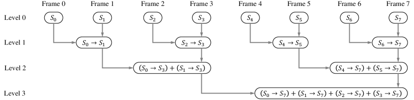
Figure 1: An example of a remapping table in the fast patch blending algorithm.

Algorithm 3 Building a remapping table

Input: $\{G_{i}\}_{i=0}^{N-1}$: guide video

Input: $\{S_{i}\}_{i=0}^{N-1}$: style video

$L_{\text{max}}\leftarrow\lceil\log_{2}N\rceil$

Initialize RemappingTable

for $i=0,1,\cdots,N-1$ do

    $\text{RemappingTable}(i,0)\leftarrow S_{i}$

    $j\leftarrow i$

    for $L=0,1,\dots,L_{\text{max}}-1$ do

         if $\text{BitwiseAnd}(i,2^{L})>0$ then

             continue

         end if

         $j\leftarrow\text{BitwiseOr}(j,2^{L})$

         if $j<N$ then

             Compute $\text{NNF}(G_{i},G_{j})$

             Compute $(S_{i}\to S_{j})$ using $\text{NNF}(G_{i},G_{j})$

             Add $(S_{i}\to S_{j})$ to $\text{RemappingTable}(j,L+1)$

         end if

    end for

end for

return RemappingTable

Algorithm 4 Building a blending table

Input: $\{G_{i}\}_{i=0}^{N-1}$: guide video

Input: $\{S_{i}\}_{i=0}^{N-1}$: style video

Computing RemappingTable using algorithm 3

$L_{\text{max}}\leftarrow\lceil\log_{2}N\rceil$

Initialize BlendingTable

for $i=0,1,\cdots,N-1$ do

    $\text{BlendingTable}(i,0)\leftarrow S_{i}$

    for $L=1,2,\dots,L_{\text{max}}-1$ do

         $\begin{aligned} \text{BlendingTable}(i,L)\leftarrow&\text{BlendingTable}(i,L-1)\\ &+\text{RemappingTable}(i,L)\end{aligned}$

    end for

end for

return BlendingTable

Algorithm 5 Query algorithm on a blending table

Input: BlendingTable

Input: $l,r$: query interval

Initialize result $A\leftarrow O$

$i\leftarrow r$

while $i\geq l$ do

    $L\leftarrow 0$

    while $\text{BitwiseAnd}(i,2^{L})>0$ and $i-2^{L+1}+1\geq l$ do

         $L\leftarrow L+1$

    end while

    Compute $\text{NNF}(G_{i},G_{r})$

    Compute $(\text{BlendingTable}(i,L)\to S_{j})$ using $\text{NNF}(G_{i},G_{r})$

    $A\leftarrow A+(\text{BlendingTable}(i,L)\to S_{j})$

end while

$A\leftarrow\frac{A}{r-l+1}$

return $A$

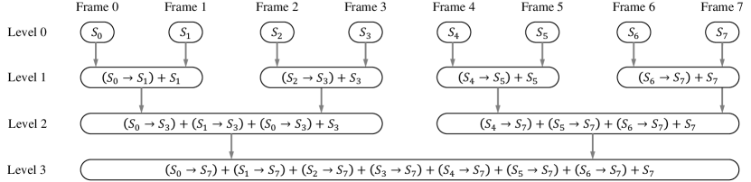
Figure 2: An example of a blending table in the fast patch blending algorithm.

In the fast patch blending algorithm, the frames are arranged in a remapping table, which is a tree-like array. An example of a remapping table is presented in Figure 1. This data structure is similar to some tree-like arrays [10, 6]. Since we have

$$(S_{i}\to S_{j})\to S_{k}\doteq S_{i}\to S_{k},$$ (4)

$$(S_{i}+S_{j})\to S_{k}\doteq(S_{i}\to S_{k})+(S_{j}\to S_{k}),$$ (5)

the remapped and blended frames can also be remapped again. In the original version of this algorithm, the remapping table is constructed within $\mathcal{O}(N)$ time complexity utilizing this conclusion. Yet, this procedure cannot be fully implemented in parallel. In practice, we find that computing each estimated NNF in parallel is faster, although the time complexity is higher. After $\mathcal{O}(N\log N)$ times of NNF estimation and image remapping, we obtain the whole remapping table. The pseudocode of constructing a remapping table is presented in Algorithm 3. Then we construct a blending table to store the prefix sum of each column. Please see Algorithm 4 and Figure 2 for more details.

After constructing the blending table, we propose a new query algorithm based on this data structure. The pseudocode is in Algorithm 5. This algorithm can compute $\frac{1}{r-l+1}\sum_{i=l}^{r}(S_{i}\to S_{r})$ within $\mathcal{O}(\log N)$ times of NNF estimation. Similarly, we use another symmetric blending table to compute $\frac{1}{r-l+1}\sum_{i=l}^{r}(S_{i}\to S_{l})$. The two intervals compose a sliding window.

$$\small\sum_{j=i-M}^{i+M}(S_{j}\to S_{i})=\sum_{j=i-M}^{i}(S_{j}\to S_{i})+\sum_{j=i}^{i+M}(S_{j}\to S_{i})-S_{i}.$$ (6)

All NNF estimation tasks in Algorithm 3 and Algorithm 5 are scheduled by a task manager. In the whole algorithm, we need $\mathcal{O}(N\log N)$ times of NNF estimation. The overall time complexity is not related to the sliding window size, making it possible to use a large sliding window.

3.4.2 Quality Improvement

When the flicker noise in a video is excessively pronounced, blending the frames together usually makes the video smoggy. This pitfall arises due to the lack of consistent remapping of content to identical positions across different frames. To overcome this pitfall, we modify the loss function to align the contents in different frames. When different source images $\{S_{i}\}_{i=0}^{N-1}$ are remapped to the same target frame $T$, $\{S_{i}\to T\}_{i=0}^{N-1}$ are supposed to be the same, otherwise the details will be discarded during the average calculation. Therefore, we first compute the average remapped image

$$\overline{T}=\frac{1}{N}\sum_{i=0}^{N-1}(S_{i}\to T).$$ (7)

Then calculate the distance between $\overline{T}$ and each remapped image. The modified loss function is formulated as

$$\mathcal{L}(S_{i},T,F_{i})_{x,y}= \alpha||S_{i}[F(x,y)]-T[x,y]||_{2}^{2}$$ (8)

$$+||S_{i}[F(x,y)]-\overline{T}[x,y]||_{2}^{2}.$$

By minimizing $||S_{i}[F(x,y)]-\overline{T}[x,y]||_{2}^{2}$, the contents are aligned together. The accurate mode requires $\mathcal{O}(NM)$ times NNF estimation and image remapping. Additionally, we do not need to construct a blending table and store all frames in RAM. Because the frames are rendered one by one, the space complexity is reduced from $\mathcal{O}(N)$ to $\mathcal{O}(M)$. Users can process long videos in accurate mode.

3.5 Interpolation

Another application scenario of FastBlend is video interpolation. To transfer the style of a video, we can render some keyframes and then use FastBlend to render the remaining frames. The keyframes can be rendered by diffusion models or GANs, and can even be painted by human artists. In this workflow, users can focus on fine-tuning the details of keyframes, thus it is easier to create fancy videos. Different from the first scenario, FastBlend doesn’t make modifications to keyframes.

3.5.1 Tracking

Considering remapping a single frame $S$ to several frames $\{T_{i}\}_{i=0}^{N-1}$ that are continuous in time, we may see high-frequency hopping on the remapped frames $\{S\to T_{i}\}_{i=0}^{N-1}$ if we compute $\{\text{NNF}(S,T_{i})\}_{i=0}^{N-1}$ using loss function (2) independently. Therefore, we decided to design an object tracking mechanism to keep the remapped frames stable. To achieve this, we use an additional step to expand the updating sequence in Algorithm 1. The $\text{NNF}(S,T_{i})$ is similar to $\text{NNF}(S,T_{i+1})$ because the adjacent frames $T_{i}$ and $T_{i+1}$ are similar, thus we add $T_{i+1}$ and $T_{i-1}$ to the updating sequence of $\text{NNF}(S,T_{i})$. The algorithm can leverage the information from $\text{NNF}(S,T_{i-1})$ and $\text{NNF}(S,T_{i+1})$ to calculate $\text{NNF}(S,T_{i})$, making the video more fluent. Additionally, the object tracking mechanism can also be applied for blending, but we do not see significant improvement in video quality. We set it to an optional setting in blending.

3.5.2 Alignment

When the number of keyframes is larger than $2$, the remaining frames $\{\tilde{S}_{i}\}_{i=l+1}^{r-1}$ between two rendered keyframes $\{S_{l},S_{r}\}$ are created according to the two keyframes. A naive method is to remap each keyframe and combine them linearly. The combined frame is formulated as

$$\tilde{S}_{i}=\frac{r-i}{r-l}(S_{l}\to S_{i})+\frac{i-l}{r-l}(S_{r}\to S_{i}).$$ (9)

However, the two remapped frames $(S_{l}\to S_{i})$ and $(S_{r}\to S_{i})$ may contain inconsistent contents. We can use the loss function (8) to align the contents in the two keyframes. To further improve the performance, we designed a fine-grained alignment loss function specially for pairwise remapping.

$$\begin{aligned} \mathcal{L}(S_{l},T,F_{l})_{x,y}=&\alpha||S_{l}[F_{l}(x,y)]-T[x,y]||_{2}^{2}\\ &+||S_{l}[F_{l}(x,y)]-S_{r}[F_{r}(x,y)]||_{2}^{2},\end{aligned}$$ (10)

$$\begin{aligned} \mathcal{L}(S_{r},T,F_{r})_{x,y}=&\alpha||S_{r}[F_{r}(x,y)]-T[x,y]||_{2}^{2}\\ &+||S_{l}[F_{l}(x,y)]-S_{r}[F_{r}(x,y)]||_{2}^{2}.\end{aligned}$$

Compared with loss function (8), the loss function (10) computes the alignment errors on patches of keyframes, not on the remapped frames. Thus, it is more accurate. This loss function is compatible with the object tracking mechanism and can be enabled at the same time.

3.6 Implementation Details

To implement an efficient toolkit, we design the following three kernel functions using C++ and compile these components to make them run on GPU.

• Remap. Remapping images in a memory-efficient way, i.e., Algorithm 2.

• Patch error. Computing the errors of matches, i.e., Algorithm 1. The loss function (2) and (8) can be implemented using this kernel function.

• Pairwise patch error. Computing the pairwise errors in 3.5.2 to implement loss function (10).

The other components of FastBlend are implemented using Python for better compatibility. To make FastBlend friendly to creators, we provide a WebUI program for interactive usage. FastBlend can also run as an extension of Stable-Diffusion-WebUI, which is the most popular UI framework of diffusion models.

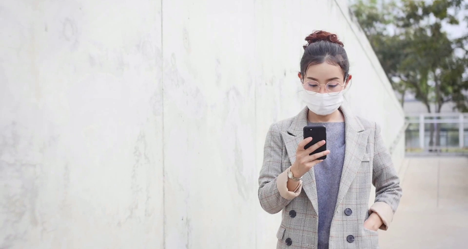
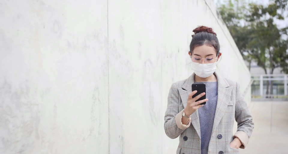
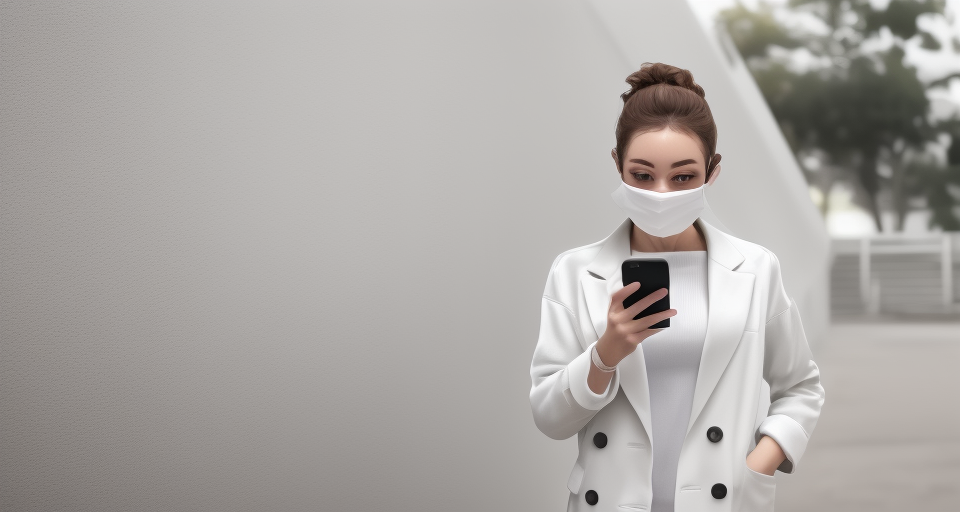
(a) Input video		(b) Naive
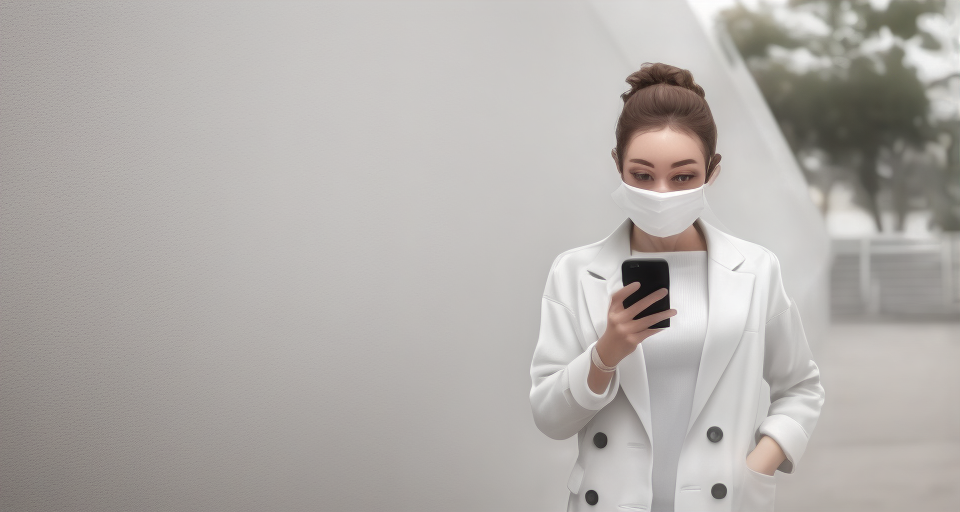
(c) FastBlend		(d) All-In-One Deflicker
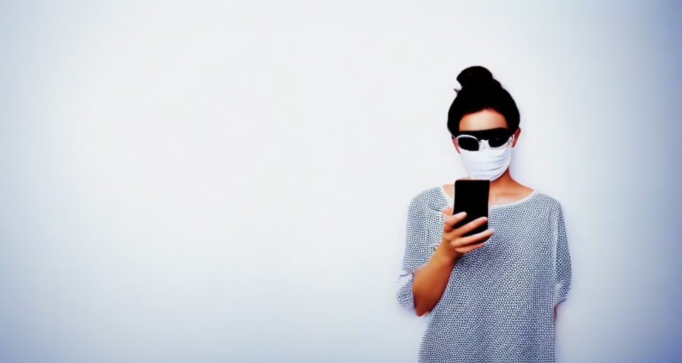
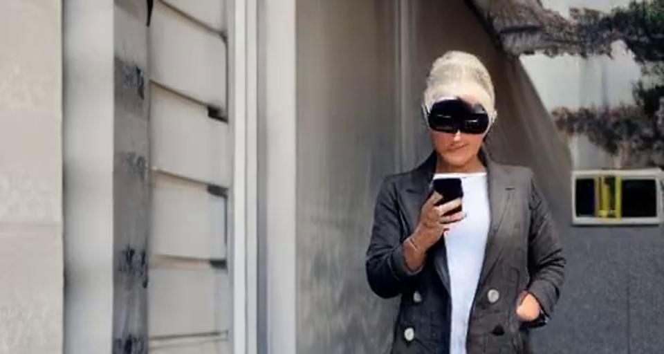
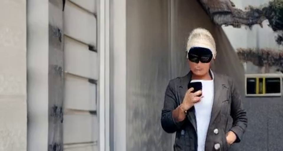
(e) Pix2Video		(f) Text2Video-Zero

Figure 3: Examples in video-to-video translation.

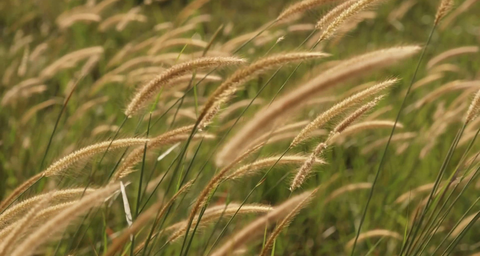
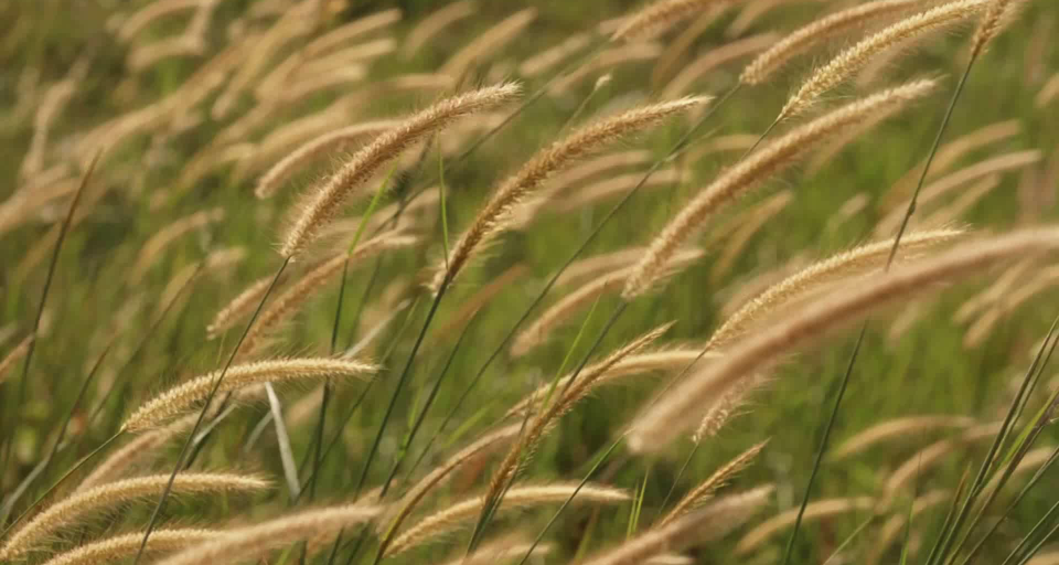
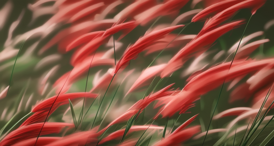
(a) First input frame	(b) Last input frame	(c) First rendered frame	(d) Last rendered frame
(e) A middle input frame	(f) FastBlend	(g) RIFE	(h) Rerender-A-Video

Figure 4: Examples in video interpolation.

(a) Guide image	(b) Style Image	(c) Input frame	(d) FastBlend
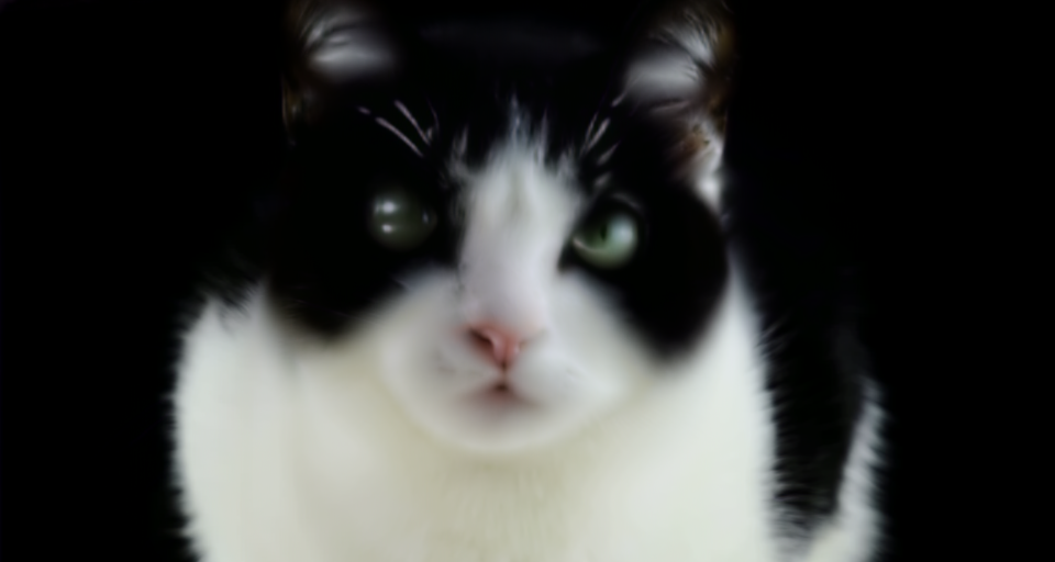
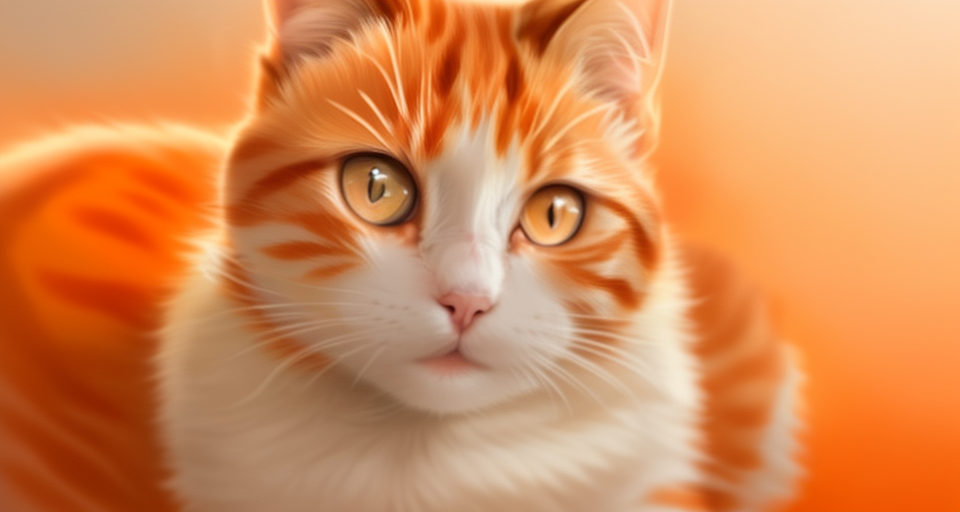
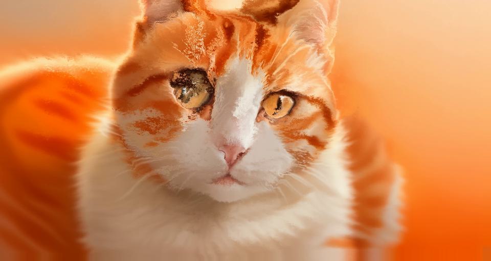
(e) Canonical image	(f) Controlling image	(g) Input frame	(h) CoDeF

Figure 5: Examples in image-driven video processing.

4 Experiments

To demonstrate the effectiveness of FastBlend, we evaluate FastBlend and other baseline methods in three tasks. Due to the lack of evaluation metrics [3, 30], we first present several video samples and then quantify the performance of FastBlend through human evaluation.

4.1 Video-to-Video Translation

Given a video and a text prompt, we transfer the style of the video according to the semantic information, while preserving the structural information. In this task, we employ the widely acclaimed diffusion model DreamShaper from open-source communities and process the entire video frame by frame. To ensure that the video inherits the original video’s structural information, we use two ControlNet [47] models, including SoftEdge and Depth. The number of sampling steps is 20, the ControlNet scale is set to 1.0, the classifier-free guidance scale [16] is 7.5, and the sampling scheduler is DDIM [38]. These hyperparameters are tuned empirically. Additionally, we enable the cross-frame attention mechanism to enhance video consistency, which is a widely proven effective trick [45, 8, 31, 5, 21]. After that, we perform post-processing on the videos using the fast blending mode in FastBlend to generate fluent videos.

An example video is shown in Figure 3, where the prompt is “a woman, mask, phone, white clothes”. Using the aforementioned diffusion model, the input video (Figure 3a) is naively processed frame by frame, and the clothes in the video turn white (Figure 3b). However, there is a noticeable inconsistency in the position of the buttons. We first compared FastBlend with All-In-One Deflicker [23], which is a state-of-the-art deflickering method. In the results of FastBlend (Figure 3c), the positions of the buttons are aligned, and the content in the two frames is consistent. In contrast, All-In-One Deflicker can only eliminate slight flickering and cannot significantly improve video consistency. Furthermore, we compared this pipeline with other video processing algorithms based on diffusion models, including Pix2Video [5] and Text2Video-Zero [21]. The results of these two baseline methods (Figure 3e and Figure 3f) also exhibit inconsistent content, such as the arms in Figure 3e and the face in Figure 3f. In this example, we demonstrate that FastBlend, combined with the diffusion model, can generate coherent and realistic videos in video-to-video translation.

4.2 Video Interpolation

Given a video, we use the diffusion model to render the first frame and the last frame, and then interpolate the content between these two frames. We employ the same diffusion model and hyperparameters as in the video-to-video translation task to render these two frames, and then use the interpolation mode in FastBlend to generate the video. We also enable the tracking mechanism from section 3.5.1 and Alignment from section 3.5.1 to enhance the coherency of the video.

An example video is shown in Figure 4, where the original video’s first frame (Figure 4a) and last frame (Figure 4b) are rendered through the diffusion model (Figure 4c and Figure 4d), respectively. We selected a middle frame from the original video (Figure 4e) for comparison of FastBlend and other methods. Due to the significant differences between the two rendered frames, this interpolation task is quite challenging. FastBlend successfully constructs a realistic image (Figure 4f). We compare FastBlend to RIFE [19], which is a video interpolation algorithm. We observe that RIFE could not generate the swaying grass, and some generated grass is even broken (Figure 4g), as it cannot fully utilize the information in the input frame (Figure 4e). Rerender-A-Video [45] also includes an interpolation algorithm based on patch matching, but it results in ghosting in the generated video (Figure 4h). This example demonstrates the effectiveness of our approach in video interpolation.

4.3 Image-Driven Video Processing

Note that the interpolation mode of FastBlend can render an entire video using only one frame, which allows users to finely adjust a single image and then extend that image’s style to the entire video. We adopted the diffusion model and experimental settings from the video-to-video translation task and validated FastBlend’s performance on this particular task.

We compare the performance of FastBlend with CoDeF [30], and an example is shown in Figure 5. For FastBlend, we only process the middle frame (Figure 5a) into a style image (Figure 5b) and then use the interpolation mode to generate the video. Alignment from 3.5.2 is disabled since there is no need to align information from multiple frames. For CoDeF, the approach starts by generating a canonical image (Figure 5e), which is then processed using the diffusion model to create a controlling image (Figure 5f) for reference. We selected a frame (Figure 5c and Figure 5g) from the original video, and the result from FastBlend (Figure 5d) is noticeably more realistic compared to CoDeF (Figure 5h), even though CoDeF’s canonical image has a closer structural resemblance to this frame.

4.4 Human Evaluation

To quantitatively evaluate FastBlend and other baseline methods in the three tasks, we conduct comparative experiments on a publicly available dataset. The dataset we used is Pixabay100 [8], which contains 100 videos collected from Pixabay along with manually written prompts. In each task, we process each video with each method according to the experimental settings mentioned above. In video interpolation, it is not feasible to apply RIFE to long videos, thus we only use the first 60 frames of each video. We invite 15 participants for a double-blind evaluation. In each evaluation round, we randomly select one of the tasks, then randomly choose a video and present the participants with videos generated by two different methods. One video is generated by FastBlend, and the other is generated by a randomly selected baseline method. The positions of these two videos were also randomized. Participants are asked to choose the video that looks best in terms of consistency and clarity or choose “tie” if the participant cannot determine which video is better.

Table 1: The results of human evaluation. Task 1 denotes video-to-video translation, task 2 denotes video interpolation and task 3 denotes image-driven video processing.

	Baseline	Which one is better
		FastBlend	Tie	Baseline
Task 1	All-In-One Deflicker	75.64%	14.10%	10.26%
	Pix2Video	91.49%	4.26%	4.26%
	Text2Video-Zero	89.44%	6.83%	3.73%
Task 2	RIFE	36.82%	31.82%	31.36%
	Rerender-A-Video	32.61%	37.83%	29.57%
Task 3	CoDeF	64.67%	16.67%	18.67%

The results of the human evaluation are shown in Table 1. In the video-to-video translation and image-driven video processing, the participants unanimously found that FastBlend’s overall performance is significantly better than the baseline methods. In the video interpolation, due to the relatively short video length, participants had difficulty observing significant differences, so FastBlend is slightly better than the baseline methods.

4.5 Efficiency Analysis

Table 2: The time consumed for processing 100 frames.

	Method	Time consumed
Task 1	All-In-One Deflicker	5.42 mins
	FastBlend	2.27 mins
Task 2	RIFE	0.09 mins
	Rerender-A-Video	3.27 mins
	FastBlend	1.15 mins
Task 3	CoDeF	4.16 mins
	FastBlend	0.67 mins

FastBlend can fully leverage GPU units. We compare the computational efficiency of these methods using an NVIDIA RTX 4090 GPU and record the time consumed for rendering 100 frames. The experimental results are shown in Table 2. Considering that Pix2Video and Text2Video-Zero are video processing methods strongly coupled with diffusion models, comparing them with other methods is unfair. In video-to-video translation and image-driven video processing tasks, FastBlend outperforms other methods significantly. In video interpolation tasks, FastBlend requires less time than Rerender-A-Video, even though both are designed based on the patch match algorithm. The video interpolation method RIFE is faster than FastBlend, but it only generates gradual effects between keyframes and cannot produce realistic motion effects. Due to the extremely high GPU utilization, FastBlend achieves both high video quality and high efficiency.

4.6 Comparison of inference modes for blending

…										…
(a) Original video
…										…
(b) Diffusion-rendered video
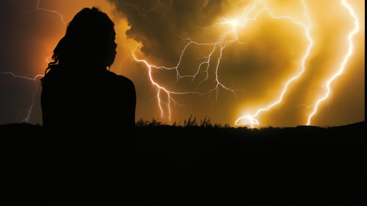
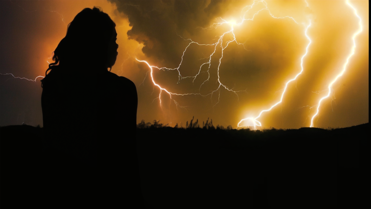
	(c) Fast mode			(d) Balanced mode			(e) Accurate mode

Figure 6: Comparison of the three inference modes for blending. Zoom in to see details.

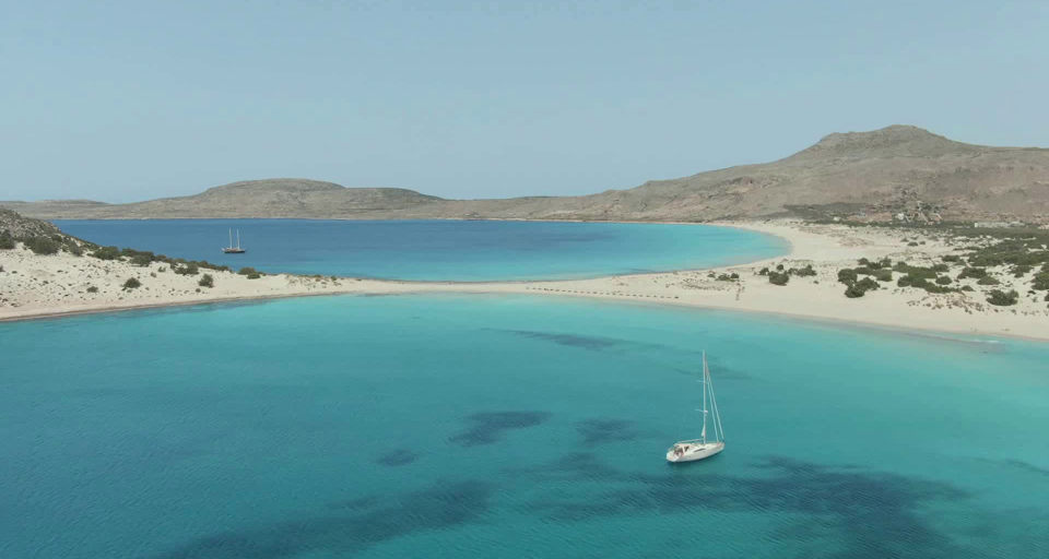
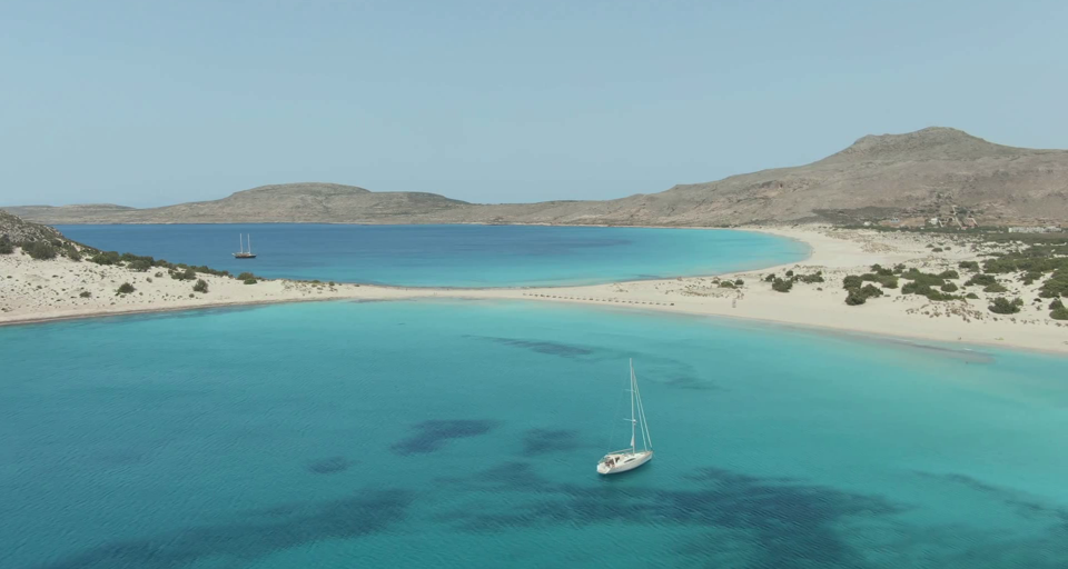
(a) Original video
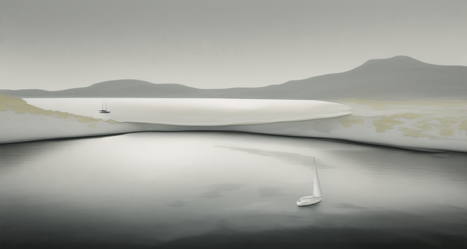
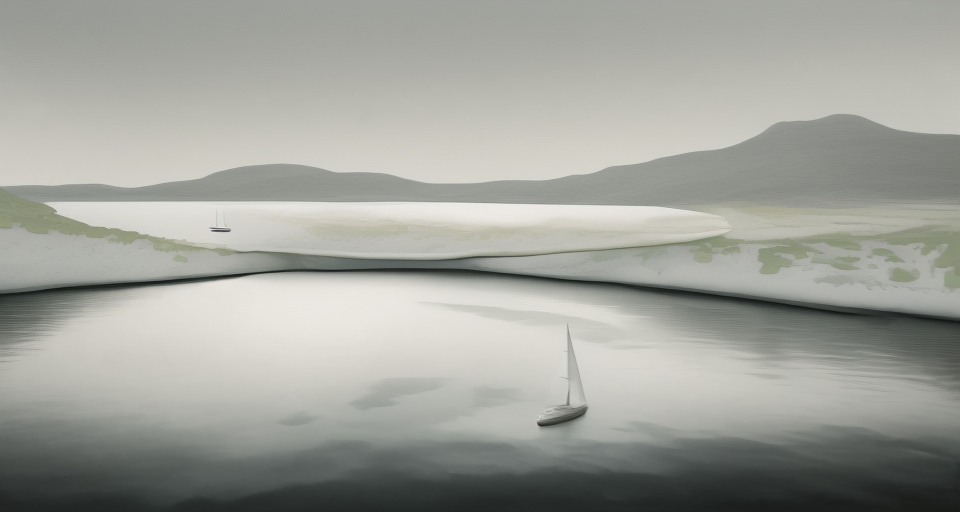
(b) The size of sliding window is 30
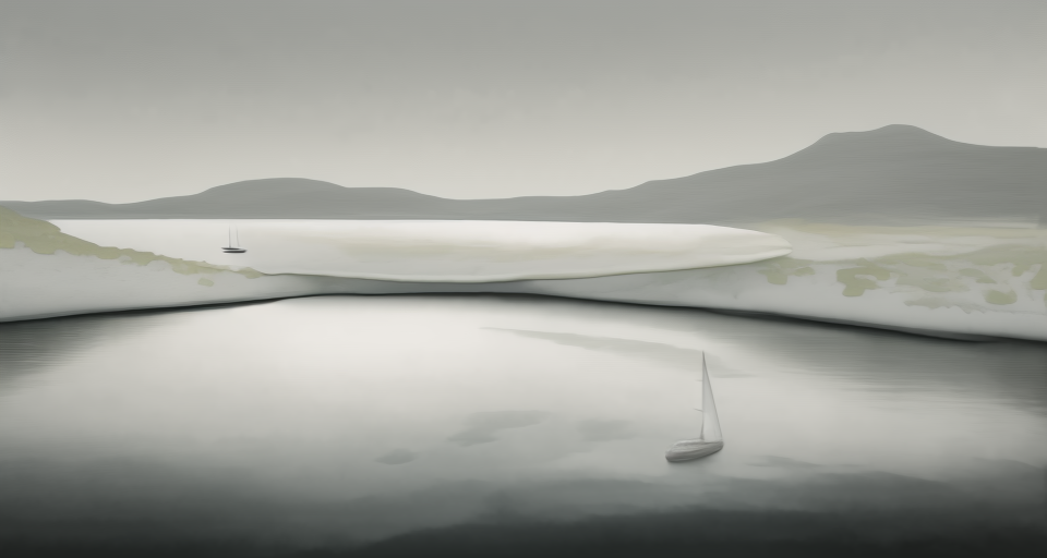
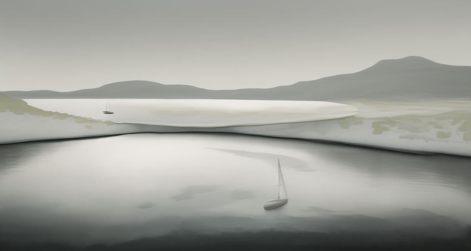
(b) The sliding window covers the whole video

Figure 7: Effect of different sizes of the sliding window.

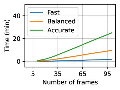
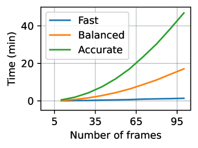
(a) The size of sliding	(b) The sliding window
window is 30	covers the whole video

Figure 8: Inference time of different inference modes for blending.

We compared the performance of different inference modes in 3.4. Figure 6 displays the results of three inference modes. The positions of lightning in the video are random and inconsistent. In the balanced mode (Figure 6d), there is a slight ghosting effect where the lightning from different frames is blended together. The ghosting issue is more pronounced in the fast mode (Figure 6c). However, in the accurate mode (Figure 6e), loss function 8 guides the optimization algorithm to remove unnecessary details and merge lightning from multiple frames into a clear frame.

We also conducted experiments to investigate the impact of different sliding window sizes. Figure 7 shows the first and last frames of a 125-frame video. When the sliding window size is set to 30 (Figure 7b), the color of the boat in the scene is different because the two frames are far apart. As the sliding window covers the entire video (Figure 7c), the color of the small boat becomes consistent. Larger sliding window sizes can improve the long-term consistency of videos but require more computation time.

Figure 8 records the computation time for three inference modes. The GPU used is an NVIDIA 4090, and the video resolution is $512\times 768$. For the balanced and accurate modes, when the sliding window size is 30, the computation time almost linearly increases with the number of frames, and when the sliding window covers the entire video, the computation time increases quadratically with the number of frames. For the fast mode, due to the linear logarithmic time complexity, the speed is very fast and is almost unaffected by the sliding window size. We also tested on a GPU with very low computing performance. We conducted tests on an NVIDIA 3060 laptop, a GPU that doesn’t even have enough VRAM to run baseline methods like Text2Video-Zero [21] and CoDeF [30]. However, FastBlend only takes 8 minutes to process 200 frames in the fast mode.

4.7 Ablation Study

4.7.1 Tracking

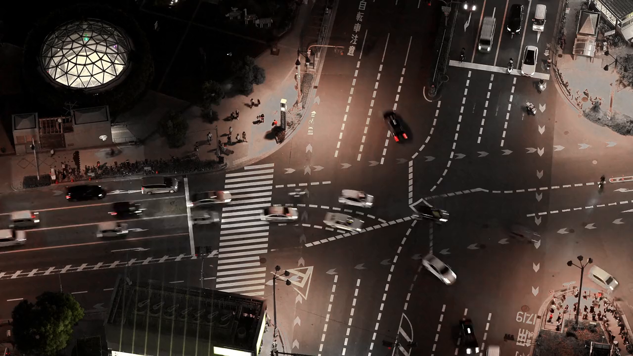
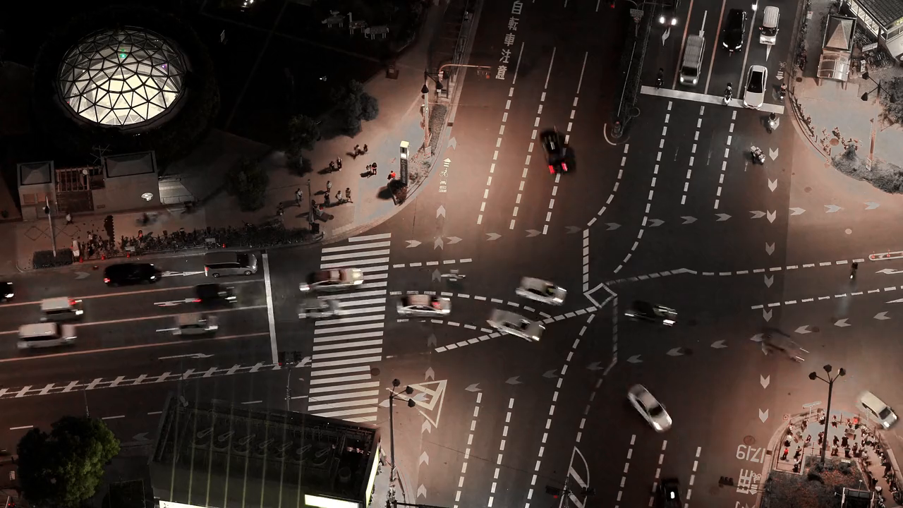
(a) Original video
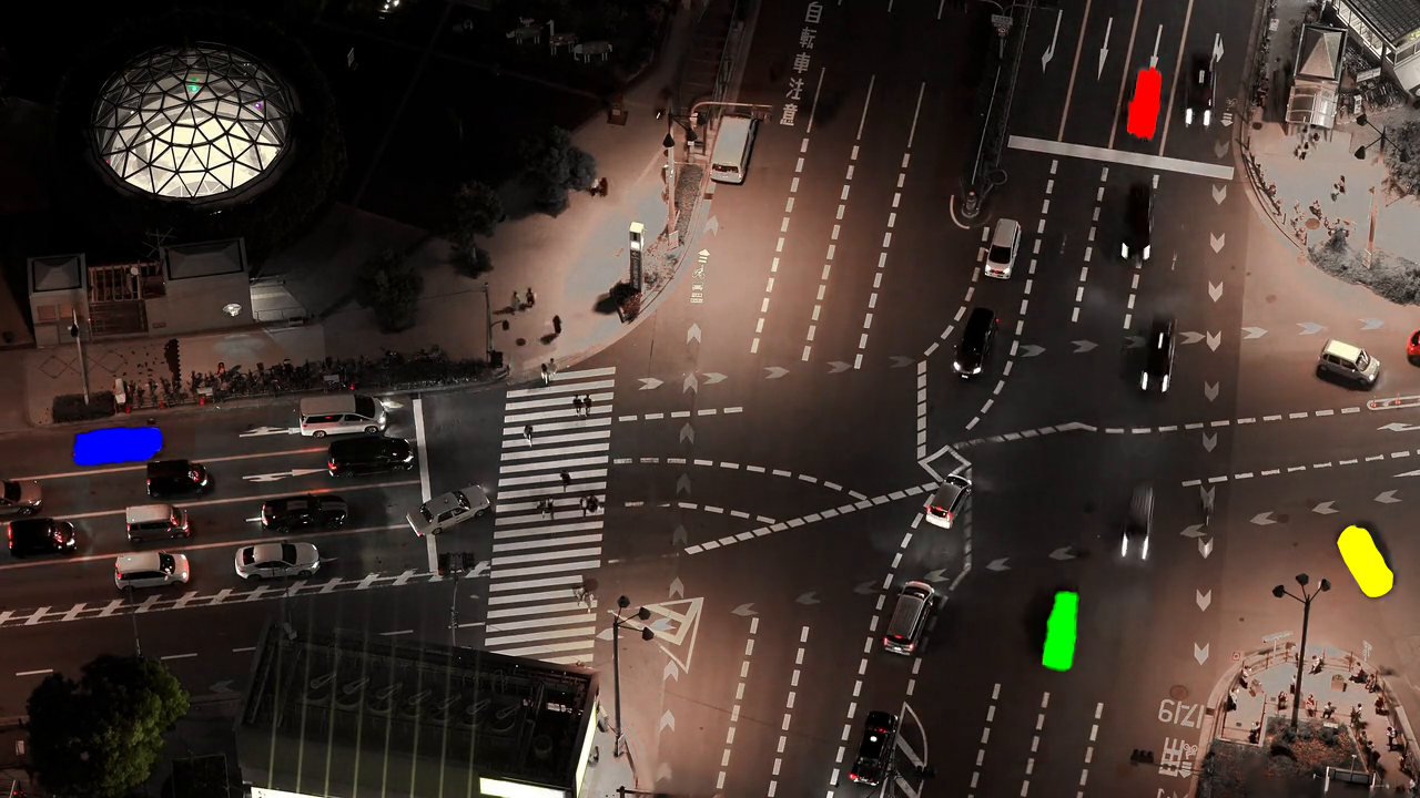
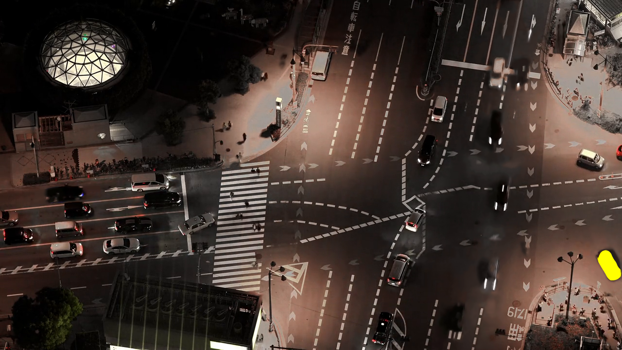
(b) Disabling the object tracking mechanism
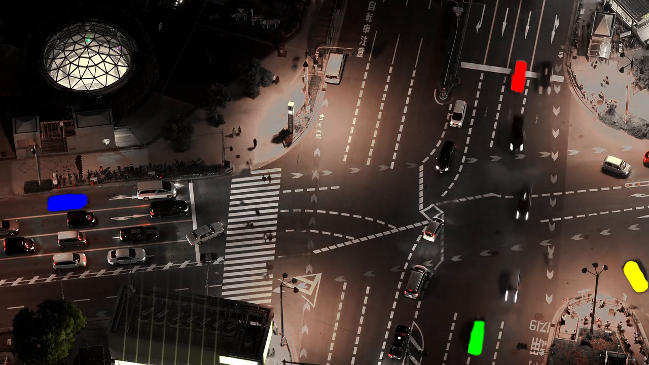
(c) Enabling the object tracking mechanism

Figure 9: Effect of the object tracking mechanism.

We evaluate the object tracking mechanism in 3.5.1. Figure 9 shows a video of a congested intersection. In the original video (Figure 3.5.1a), there are many vehicles. In the first frame, we select four moving cars and color them differently, and then we use the first frame as a keyframe to render this video. When the object tracking mechanism is disabled (Figure 3.5.1b), the colors of the four cars quickly fade away. However, when the object tracking mechanism is enabled (Figure 3.5.1c), the colors on the four cars remain stable. This tracking mechanism can enhance the stability of rendering videos. However, this mechanism is only designed for NNF estimation and is not a general-purpose tracking algorithm. We do not recommend using this tracking mechanism for general tracking tasks, because it is not widely evaluated on general tracking tasks and is less robust compared to some prior general approaches [41, 18].

4.7.2 Alignment

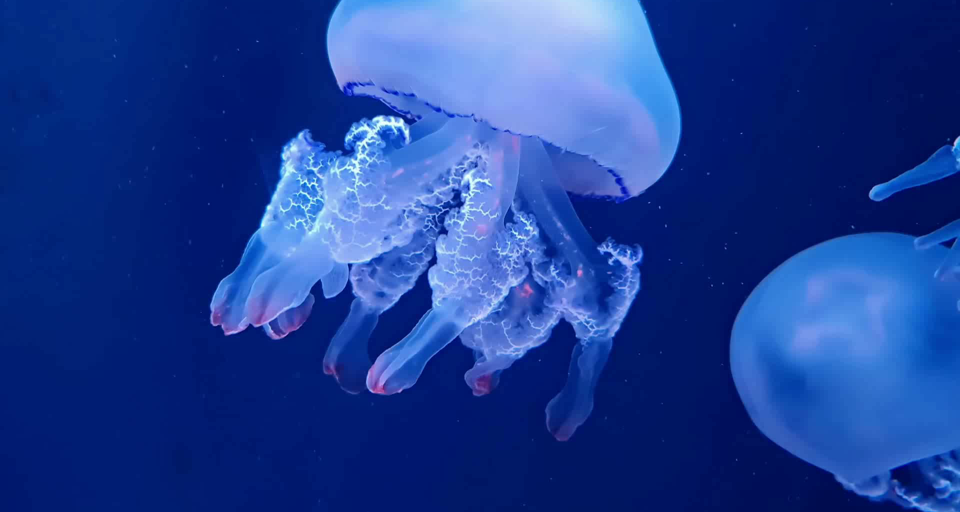
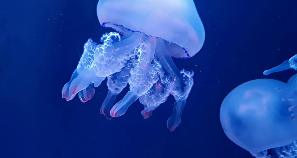
(a) Keyframes
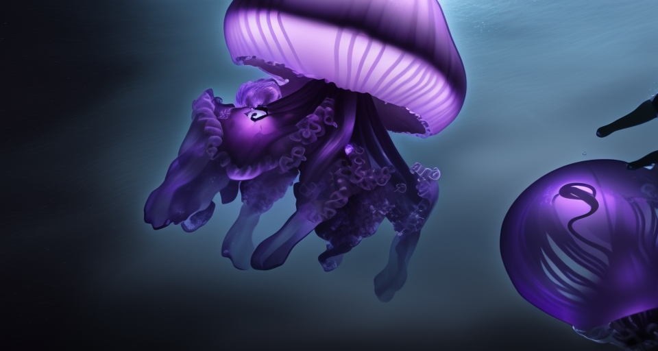
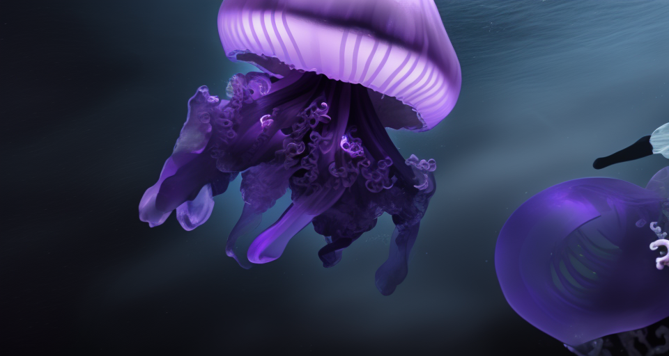
(b) Diffusion-rendered keyframes
(c) Interpolated frame	(d) Interpolated frame
without alignment	with alignment

Figure 10: Effect of the alignment mechanism.

Figure 10 illustrates the effect of the alignment mechanism in 3.5.2. After rendering the jellyfish in two keyframes (Figure 10a) into purple (Figure 10b), inconsistent content appears in the bottom right corner of the video. When we generate the intermediate frame in interpolation mode without the alignment mechanism (Figure 10c), the inconsistent content transparently overlays. When we generate the intermediate frames with the alignment mechanism, the inconsistent content is eliminated. The alignment mechanism effectively integrates the content from two inconsistent keyframes.

5 Conclusion

In this paper, we propose a model-free video processing toolkit called FastBlend. FastBlend can be combined with diffusion models to create powerful video processing pipelines. FastBlend can effectively eliminate flicker in videos, interpolate keyframe sequences, and even process complete videos based on a single image. Extensive experimental results have demonstrated the superiority of FastBlend. In the future, we intend to integrate FastBlend with other video processing methods to build more powerful video processing tools.

References

- Bar-Tal et al. [2022] Omer Bar-Tal, Dolev Ofri-Amar, Rafail Fridman, Yoni Kasten, and Tali Dekel. Text2live: Text-driven layered image and video editing. In European conference on computer vision, pages 707–723. Springer, 2022.
- Barnes et al. [2009] Connelly Barnes, Eli Shechtman, Adam Finkelstein, and Dan B Goldman. Patchmatch: A randomized correspondence algorithm for structural image editing. ACM Trans. Graph., 28(3):24, 2009.
- Brooks et al. [2022] Tim Brooks, Janne Hellsten, Miika Aittala, Ting-Chun Wang, Timo Aila, Jaakko Lehtinen, Ming-Yu Liu, Alexei Efros, and Tero Karras. Generating long videos of dynamic scenes. Advances in Neural Information Processing Systems, 35:31769–31781, 2022.
- Brooks et al. [2023] Tim Brooks, Aleksander Holynski, and Alexei A Efros. Instructpix2pix: Learning to follow image editing instructions. In Proceedings of the IEEE/CVF Conference on Computer Vision and Pattern Recognition, pages 18392–18402, 2023.
- Ceylan et al. [2023] Duygu Ceylan, Chun-Hao P Huang, and Niloy J Mitra. Pix2video: Video editing using image diffusion. In Proceedings of the IEEE/CVF International Conference on Computer Vision, pages 23206–23217, 2023.
- De Berg [2000] Mark De Berg. Computational geometry: algorithms and applications. Springer Science & Business Media, 2000.
- Dhariwal and Nichol [2021] Prafulla Dhariwal and Alexander Nichol. Diffusion models beat gans on image synthesis. Advances in neural information processing systems, 34:8780–8794, 2021.
- Duan et al. [2023] Zhongjie Duan, Lizhou You, Chengyu Wang, Cen Chen, Ziheng Wu, Weining Qian, and Jun Huang. Diffsynth: Latent in-iteration deflickering for realistic video synthesis. arXiv preprint arXiv:2308.03463, 2023.
- Esser et al. [2023] Patrick Esser, Johnathan Chiu, Parmida Atighehchian, Jonathan Granskog, and Anastasis Germanidis. Structure and content-guided video synthesis with diffusion models. In Proceedings of the IEEE/CVF International Conference on Computer Vision, pages 7346–7356, 2023.
- Fenwick [1994] Peter M Fenwick. A new data structure for cumulative frequency tables. Software: Practice and experience, 24(3):327–336, 1994.
- Gal et al. [2022] Rinon Gal, Yuval Alaluf, Yuval Atzmon, Or Patashnik, Amit Haim Bermano, Gal Chechik, and Daniel Cohen-or. An image is worth one word: Personalizing text-to-image generation using textual inversion. In The Eleventh International Conference on Learning Representations, 2022.
- Goodfellow et al. [2014] Ian Goodfellow, Jean Pouget-Abadie, Mehdi Mirza, Bing Xu, David Warde-Farley, Sherjil Ozair, Aaron Courville, and Yoshua Bengio. Generative adversarial nets. Advances in neural information processing systems, 27, 2014.
- Grover and Lin [2012] Vinod Grover and Yuan Lin. Compiling cuda and other languages for gpus. In GPU Technology Conference (GTC), pages 1–59, 2012.
- Guo et al. [2021] Xiefan Guo, Hongyu Yang, and Di Huang. Image inpainting via conditional texture and structure dual generation. In Proceedings of the IEEE/CVF International Conference on Computer Vision, pages 14134–14143, 2021.
- Hertz et al. [2022] Amir Hertz, Ron Mokady, Jay Tenenbaum, Kfir Aberman, Yael Pritch, and Daniel Cohen-or. Prompt-to-prompt image editing with cross-attention control. In The Eleventh International Conference on Learning Representations, 2022.
- Ho and Salimans [2021] Jonathan Ho and Tim Salimans. Classifier-free diffusion guidance. In NeurIPS 2021 Workshop on Deep Generative Models and Downstream Applications, 2021.
- Hu et al. [2021] Edward J Hu, Phillip Wallis, Zeyuan Allen-Zhu, Yuanzhi Li, Shean Wang, Lu Wang, Weizhu Chen, et al. Lora: Low-rank adaptation of large language models. In International Conference on Learning Representations, 2021.
- Huang et al. [2020] Lianghua Huang, Xin Zhao, and Kaiqi Huang. Globaltrack: A simple and strong baseline for long-term tracking. In Proceedings of the AAAI Conference on Artificial Intelligence, pages 11037–11044, 2020.
- Huang et al. [2022] Zhewei Huang, Tianyuan Zhang, Wen Heng, Boxin Shi, and Shuchang Zhou. Real-time intermediate flow estimation for video frame interpolation. In European Conference on Computer Vision, pages 624–642. Springer, 2022.
- Jamriška et al. [2019] Ondřej Jamriška, Šárka Sochorová, Ondřej Texler, Michal Lukáč, Jakub Fišer, Jingwan Lu, Eli Shechtman, and Daniel Sỳkora. Stylizing video by example. ACM Transactions on Graphics (TOG), 38(4):1–11, 2019.
- Khachatryan et al. [2023] Levon Khachatryan, Andranik Movsisyan, Vahram Tadevosyan, Roberto Henschel, Zhangyang Wang, Shant Navasardyan, and Humphrey Shi. Text2video-zero: Text-to-image diffusion models are zero-shot video generators. arXiv preprint arXiv:2303.13439, 2023.
- Kochura et al. [2020] Yuriy Kochura, Yuri Gordienko, Vlad Taran, Nikita Gordienko, Alexandr Rokovyi, Oleg Alienin, and Sergii Stirenko. Batch size influence on performance of graphic and tensor processing units during training and inference phases. In Advances in Computer Science for Engineering and Education II, pages 658–668. Springer, 2020.
- Lei et al. [2023] Chenyang Lei, Xuanchi Ren, Zhaoxiang Zhang, and Qifeng Chen. Blind video deflickering by neural filtering with a flawed atlas. In Proceedings of the IEEE/CVF Conference on Computer Vision and Pattern Recognition, pages 10439–10448, 2023.
- Li et al. [2022] Haoying Li, Yifan Yang, Meng Chang, Shiqi Chen, Huajun Feng, Zhihai Xu, Qi Li, and Yueting Chen. Srdiff: Single image super-resolution with diffusion probabilistic models. Neurocomputing, 479:47–59, 2022.
- Liu et al. [2021] Steven Liu, Xiuming Zhang, Zhoutong Zhang, Richard Zhang, Jun-Yan Zhu, and Bryan Russell. Editing conditional radiance fields. In Proceedings of the IEEE/CVF international conference on computer vision, pages 5773–5783, 2021.
- Luebke [2008] David Luebke. Cuda: Scalable parallel programming for high-performance scientific computing. In 2008 5th IEEE international symposium on biomedical imaging: from nano to macro, pages 836–838. IEEE, 2008.
- Meng et al. [2021] Chenlin Meng, Yutong He, Yang Song, Jiaming Song, Jiajun Wu, Jun-Yan Zhu, and Stefano Ermon. Sdedit: Guided image synthesis and editing with stochastic differential equations. In International Conference on Learning Representations, 2021.
- Mou et al. [2023] Chong Mou, Xintao Wang, Liangbin Xie, Jian Zhang, Zhongang Qi, Ying Shan, and Xiaohu Qie. T2i-adapter: Learning adapters to dig out more controllable ability for text-to-image diffusion models. arXiv preprint arXiv:2302.08453, 2023.
- Mount [2010] David M Mount. Ann: A library for approximate nearest neighbor searching. http://www. cs. umd. edu/~ mount/ANN/, 2010.
- Ouyang et al. [2023] Hao Ouyang, Qiuyu Wang, Yuxi Xiao, Qingyan Bai, Juntao Zhang, Kecheng Zheng, Xiaowei Zhou, Qifeng Chen, and Yujun Shen. Codef: Content deformation fields for temporally consistent video processing. arXiv preprint arXiv:2308.07926, 2023.
- Qi et al. [2023] Chenyang Qi, Xiaodong Cun, Yong Zhang, Chenyang Lei, Xintao Wang, Ying Shan, and Qifeng Chen. Fatezero: Fusing attentions for zero-shot text-based video editing. arXiv preprint arXiv:2303.09535, 2023.
- Ramesh et al. [2022] Aditya Ramesh, Prafulla Dhariwal, Alex Nichol, Casey Chu, and Mark Chen. Hierarchical text-conditional image generation with clip latents. arXiv preprint arXiv:2204.06125, 1(2):3, 2022.
- Rombach et al. [2022] Robin Rombach, Andreas Blattmann, Dominik Lorenz, Patrick Esser, and Björn Ommer. High-resolution image synthesis with latent diffusion models. In Proceedings of the IEEE/CVF conference on computer vision and pattern recognition, pages 10684–10695, 2022.
- Ruiz et al. [2023] Nataniel Ruiz, Yuanzhen Li, Varun Jampani, Yael Pritch, Michael Rubinstein, and Kfir Aberman. Dreambooth: Fine tuning text-to-image diffusion models for subject-driven generation. In Proceedings of the IEEE/CVF Conference on Computer Vision and Pattern Recognition, pages 22500–22510, 2023.
- Saharia et al. [2022] Chitwan Saharia, William Chan, Saurabh Saxena, Lala Li, Jay Whang, Emily L Denton, Kamyar Ghasemipour, Raphael Gontijo Lopes, Burcu Karagol Ayan, Tim Salimans, et al. Photorealistic text-to-image diffusion models with deep language understanding. Advances in Neural Information Processing Systems, 35:36479–36494, 2022.
- Schuhmann et al. [2022] Christoph Schuhmann, Romain Beaumont, Richard Vencu, Cade Gordon, Ross Wightman, Mehdi Cherti, Theo Coombes, Aarush Katta, Clayton Mullis, Mitchell Wortsman, et al. Laion-5b: An open large-scale dataset for training next generation image-text models. arXiv preprint arXiv:2210.08402, 2022.
- Singer et al. [2022] Uriel Singer, Adam Polyak, Thomas Hayes, Xi Yin, Jie An, Songyang Zhang, Qiyuan Hu, Harry Yang, Oron Ashual, Oran Gafni, et al. Make-a-video: Text-to-video generation without text-video data. In The Eleventh International Conference on Learning Representations, 2022.
- Song et al. [2020] Jiaming Song, Chenlin Meng, and Stefano Ermon. Denoising diffusion implicit models. In International Conference on Learning Representations, 2020.
- Teed and Deng [2020] Zachary Teed and Jia Deng. Raft: Recurrent all-pairs field transforms for optical flow. In Computer Vision–ECCV 2020: 16th European Conference, Glasgow, UK, August 23–28, 2020, Proceedings, Part II 16, pages 402–419. Springer, 2020.
- Wang et al. [2021] Xintao Wang, Liangbin Xie, Chao Dong, and Ying Shan. Real-esrgan: Training real-world blind super-resolution with pure synthetic data. In Proceedings of the IEEE/CVF international conference on computer vision, pages 1905–1914, 2021.
- Wojke et al. [2017] Nicolai Wojke, Alex Bewley, and Dietrich Paulus. Simple online and realtime tracking with a deep association metric. In 2017 IEEE international conference on image processing (ICIP), pages 3645–3649. IEEE, 2017.
- Wu et al. [2023] Jay Zhangjie Wu, Yixiao Ge, Xintao Wang, Stan Weixian Lei, Yuchao Gu, Yufei Shi, Wynne Hsu, Ying Shan, Xiaohu Qie, and Mike Zheng Shou. Tune-a-video: One-shot tuning of image diffusion models for text-to-video generation. In Proceedings of the IEEE/CVF International Conference on Computer Vision, pages 7623–7633, 2023.
- Xing et al. [2023] Zhen Xing, Qijun Feng, Haoran Chen, Qi Dai, Han Hu, Hang Xu, Zuxuan Wu, and Yu-Gang Jiang. A survey on video diffusion models. arXiv preprint arXiv:2310.10647, 2023.
- Yang et al. [2022] Ling Yang, Zhilong Zhang, Yang Song, Shenda Hong, Runsheng Xu, Yue Zhao, Wentao Zhang, Bin Cui, and Ming-Hsuan Yang. Diffusion models: A comprehensive survey of methods and applications. ACM Computing Surveys, 2022.
- Yang et al. [2023] Shuai Yang, Yifan Zhou, Ziwei Liu, and Chen Change Loy. Rerender a video: Zero-shot text-guided video-to-video translation. arXiv preprint arXiv:2306.07954, 2023.
- Yu et al. [2021] Sihyun Yu, Jihoon Tack, Sangwoo Mo, Hyunsu Kim, Junho Kim, Jung-Woo Ha, and Jinwoo Shin. Generating videos with dynamics-aware implicit generative adversarial networks. In International Conference on Learning Representations, 2021.
- Zhang et al. [2023] Lvmin Zhang, Anyi Rao, and Maneesh Agrawala. Adding conditional control to text-to-image diffusion models. In Proceedings of the IEEE/CVF International Conference on Computer Vision, pages 3836–3847, 2023.
- Zhou et al. [2022] Shangchen Zhou, Kelvin Chan, Chongyi Li, and Chen Change Loy. Towards robust blind face restoration with codebook lookup transformer. Advances in Neural Information Processing Systems, 35:30599–30611, 2022.